2.8

BASIC MOLECULAR DYNAMICS

Ju LiDepartment of Materials Science and Engineering,Ohio State University, Columbus, OH, USA

A working definition of molecular dynamics (MD) simulation is techniqueby which one generates the atomic trajectories of a system of N particlesby numerical integration of Newton’s equation of motion, for a specificinteratomic potential, with certain initial condition (IC) and boundarycondition (BC).

Consider, for example (see Fig. 1), a system with N atoms in a volume �.We can define its internal energy: E ≡ K + U , where K is the kinetic energy,

K ≡N∑

i=1

1

2mi |xi (t)|2, (1)

and U is the potential energy,

U = U (x3N (t)). (2)

x3N (t) denotes the collective of 3 D coordinates x1(t), x2(t), . . . , xN (t).Note that E should be a conserved quantity, i.e., a constant of time, if thesystem is truly isolated.

One can often treat a MD simulation like an experiment. Below is acommon flowchart of an ordinary MD run:

[system setup] [equilibration] [simulation run] [output]sample selection → sample preparation → property average → data analysis(pot., N , IC, BC) (achieve T, P) (run L steps) (property calc.)

in which we fine-tune the system until it reaches the desired condition (here,temperature T and pressure P), and then perform property averages, forinstance calculating the radial distribution function g(r) [1] or thermal con-ductivity [2]. One may also perform a non-equilibrium MD calculation, duringwhich the system is subjected to perturbational or large external driving forces,

565S. Yip (ed.),Handbook of Materials Modeling, 565–588.c© 2005 Springer. Printed in the Netherlands.

566 J. Li

x

xi(t)

y

N particles

z

Figure 1. Illustration of the MD simulation system.

and we analyze its non-equilibrium response, such as in many mechanicaldeformation simulations.

There are five key ingredients to a MD simulation, which are boundarycondition, initial condition, force calculation, integrator/ensemble, and prop-erty calculation. A brief overview of them is given below, followed by morespecific discussions.

Boundary condition. There are two major types of boundary conditions:isolated boundary condition (IBC) and periodic boundary condition (PBC).IBC is ideally suited for studying clusters and molecules, while PBC is suitedfor studying bulk liquids and solids. There could also be mixed boundary con-ditions such as slab or wire configurations for which the system is assumed tobe periodic in some directions but not in the others.

In IBC, the N -particle system is surrounded by vacuum; these particlesinteract among themselves, but are presumed to be so far away from every-thing else in the universe that no interactions with the outside occur exceptperhaps responding to some well-defined “external forcing.” In PBC, one expl-icitly keeps track of the motion of N particles in the so-called supercell, butthe supercell is surrounded by infinitely replicated, periodic images of itself.Therefore a particle may interact not only with particles in the same supercellbut also with particles in adjacent image supercells (Fig. 2).

While several polyhedron shapes (such as hexagonal prism and rhombicdodecahedron from Wigner–Seitz construction) can be used as the space-fillingunit and thus can serve as the PBC supercell, the simplest and most often usedsupercell shape is a parallelepiped, specified by its three edge vectors h1, h2

and h3. It should be noted that IBC can often be well mimicked by a largeenough PBC supercell so the images do not interact.

Initial condition. Since Newton’s equations of motion are second-orderordinary differential equations (ODE), IC basically means x3N (t = 0) and

Basic molecular dynamics 567

h2 h1

rc

Figure 2. Illustration of periodic boundary condition (PBC). We explicitly keep track oftrajectories of only the atoms in the center cell called the supercell (defined by edge vectorsh1, h2 and h3), which is infinitely replicated in all three directions (image supercells). Anatom in the supercell may interact with other atoms in the supercell as well as atoms in thesurrounding image supercells. rc is a cut-off distance of the interatomic potential, beyond whichinteraction may be safely ignored.

x3N (t = 0), the initial particle positions and velocities. Generating the IC forcrystalline solids is usually quite easy, but IC for liquids needs some work,and even more so for amorphous solids. A common strategy to create a properliquid configuration is to melt a crystalline solid. And if one wants toobtain an amorphous configuration, a strategy is to quench the liquid during aMD run.

Let us focus on IC for crystalline solids. For instance, x3N (t = 0) can bea fcc perfect crystal (assuming PBC), or an interface between two crystallinephases. For most MD simulations, one needs to write an initial structure gen-eration subroutine. Before feeding the initial configuration thus created into aMD run, it is a good idea to visualize it first, checking bond lengths and coor-dination numbers, etc. [3]. A frequent cause of MD simulation breakdown ispathological initial condition, as the atoms are too close to each other initially,leading to huge forces.

According to the equipartition theorem [4], each independent degree offreedom should possess kBT/2 kinetic energy. So, one should draw each

568 J. Li

component of the 3N -dimensional x3N (t =0) vector from a Gaussian–Maxwellnormal distribution N(0, kBT/mi). After that, it is a good idea to eliminate thecenter of mass velocity, and for clusters, the net angular momentum as well.

Force calculation. Before moving into the details of force calculation, itshould be mentioned that two approximations underly the use of the classicalequation of motion

mid2xi(t)

dt2= fi ≡ −∂U

∂xi, i = 1, . . . , N (3)

to describe the atoms. The first is the Born–Oppenheimer approximation [5]which assumes the electronic state couples adiabatically to nuclei motion. Thesecond is that the nucleus motion is far removed from the Heisenberg uncer-tainty lower bound: �E�t � h/2. If we plug in �E = kBT/2, the kineticenergy, and �t = 1/ω, where ω is a characteristic vibrational frequency, weobtain kBT/hω � 1. In solids, this means the temperature should be signifi-cantly greater than the Debye temperature, which is actually quite a stringentrequirement. Indeed, large deviations from experimental heat capacities areseen in classical MD simulations of crystalline solids [2]. A variety of schemesexist to correct this error [1], for instance the Wigner–Kirkwood expansion [6]and path integral molecular dynamics [7].

The evaluation of the right-hand side of Eq. (3) is the key step that usu-ally consumes most of the computational time in a MD simulation, so itsefficiency is crucial. For long-range Coulomb interactions, special algorithmsexist to break them up into two contributions: a short-ranged interaction, plusa smooth, field-like interaction, both of which can be computed efficiently inseparate ways [8]. In this article we focus on issues concerning short-rangeinteractions only. There is a section about the Lennard–Jones potential and itstrunction schemes, followed by a section about how to construct and main-tain an atom–atom neighborlist with O(N) computational effort per timestep.Finally, see Chap. 2.2–2.6 for the development of interatomic potentialfunctions.

Integrator/ensemble. Equation (3) is a set of second-order ODEs, whichcan be strongly nonlinear. By converting them to first-order ODEs in the 6N -dimensional space of {xN , xN }, general numerical algorithms for solving ODEssuch as the Runge–Kutta method [9] can be applied. However, these gen-eral methods are rarely used in MD, because the existence of a Hamilto-nian allows for more accurate integration algorithms, prominent among whichare the family of predictor-corrector integrators [10] and the family of sym-plectic integrators [8, 11]. A section in this article gives a brief overview ofintegrators.

Ensembles such as the micro-canonical, canonical, and grand-canonical areconcepts in statistical physics that refer to the distribution of initial conditions.A system, once drawn from a certain ensemble, is supposed to follow strictly

Basic molecular dynamics 569

the Hamiltonian equation of motion Eq. (3), with E conserved. However,ensemble and integrator are often grouped together because there exists a classof methods that generates the desired ensemble distribution via time integra-tion [12, 13]. Equation (3) is modified in these methods to create a specialdynamics whose trajectory over time forms a cloud in phase space that hasthe desired distribution density. Thus, the time-average of a single-point oper-ator in one such trajectory approaches the thermodynamic average. However,one should be careful in using it to calculate two-point correlation functionaverages. See Chap. 2.9 for detailed description of these methods.

Property calculation. A great value of MD simulation is that it is “omn-ipotent” at the level of classical atoms. All properties that are well-posed inclassical mechanics and statistical mechanics can in principle be computed.The issues remaining are accuracy (the error comes from the interatomicpotential) and computational efficiency. The properties can be roughly groupedinto four categories:

1. Structural characterization. Examples include radial distribution func-tion, dynamic structure factor, etc.

2. Equation of state. Examples include free-energy functions, phase dia-grams, static response functions like thermal expansion coefficient, etc.

3. Transport. Examples include viscosity, thermal conductivity (electroniccontribution excluded), correlation functions, diffusivity, etc.

4. Non-equilibrium response. Examples include plastic deformation, pat-tern formation, etc.

1. The Lennard–Jones Potential

The solid and liquid states of rare-gas elements Ne, Ar, Kr, Xe are betterunderstood than other elements because their closed-shell electron configura-tions do not allow them to participate in covalent or metallic bonding withneighbors, which are strong and complex, but only to interact via weak vander Waals bonds, which are perturbational in nature in these elements andtherefore mostly additive, leading to the pair-potential model:

U (x3N ) =N∑

j>i

V (|x j i |), x j i ≡ x j − xi , (4)

where we assert that the total potential energy can be decomposed into the dir-ect sum of individual “pair-interactions.” If there is to be rotational invariancein U (x3N ), V can only depend on r j i ≡ |x j i |. In particular, the Lennard–Jonespotential

V (r) = 4ε

[(σ

r

)12

−(

σ

r

)6], (5)

570 J. Li

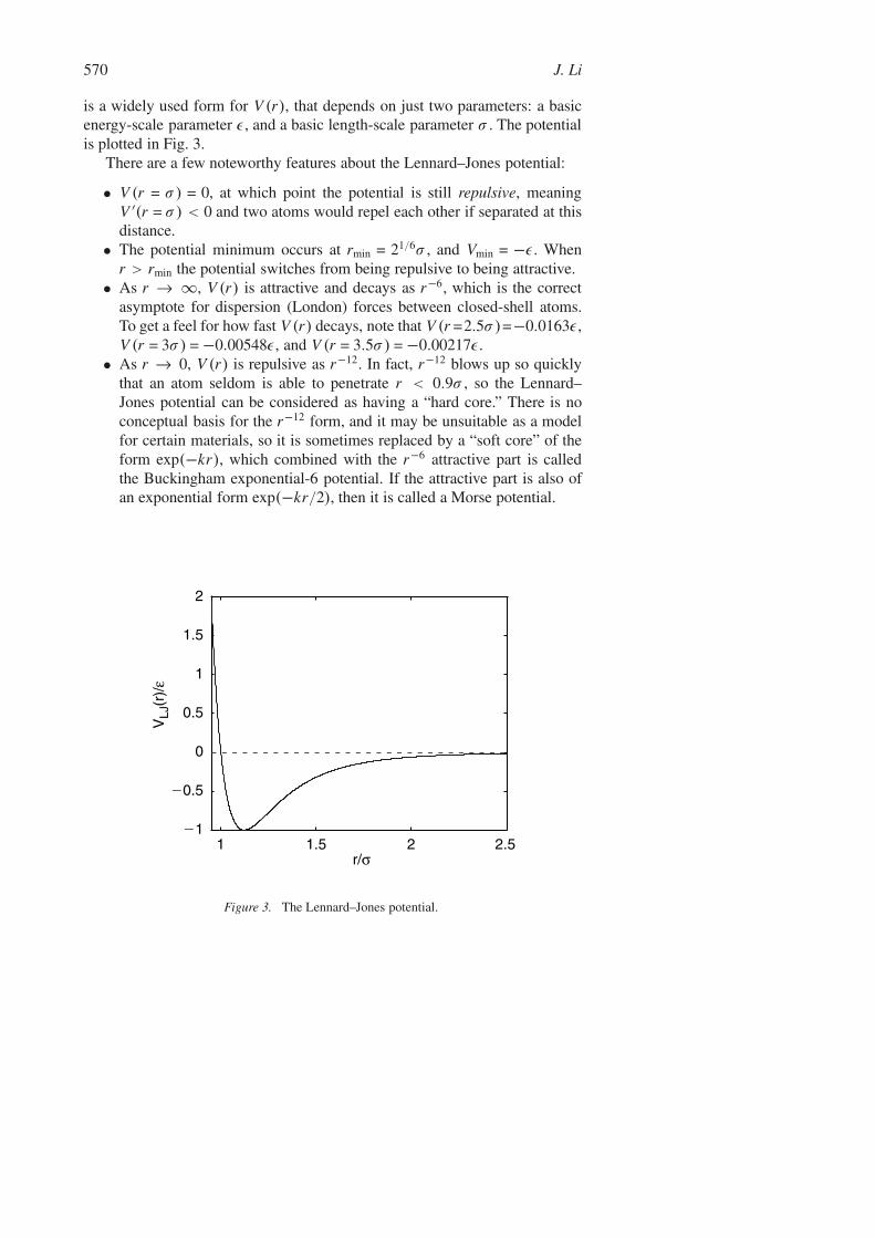
is a widely used form for V (r), that depends on just two parameters: a basicenergy-scale parameter ε, and a basic length-scale parameter σ . The potentialis plotted in Fig. 3.

There are a few noteworthy features about the Lennard–Jones potential:

• V (r = σ ) = 0, at which point the potential is still repulsive, meaningV ′(r = σ ) < 0 and two atoms would repel each other if separated at thisdistance.

• The potential minimum occurs at rmin = 21/6σ , and Vmin = −ε. Whenr > rmin the potential switches from being repulsive to being attractive.

• As r → ∞, V (r) is attractive and decays as r−6, which is the correctasymptote for dispersion (London) forces between closed-shell atoms.To get a feel for how fast V (r) decays, note that V (r =2.5σ )=−0.0163ε,V (r = 3σ ) = −0.00548ε, and V (r = 3.5σ ) = −0.00217ε.

• As r → 0, V (r) is repulsive as r−12. In fact, r−12 blows up so quicklythat an atom seldom is able to penetrate r < 0.9σ , so the Lennard–Jones potential can be considered as having a “hard core.” There is noconceptual basis for the r−12 form, and it may be unsuitable as a modelfor certain materials, so it is sometimes replaced by a “soft core” of theform exp(−kr), which combined with the r−6 attractive part is calledthe Buckingham exponential-6 potential. If the attractive part is also ofan exponential form exp(−kr/2), then it is called a Morse potential.

1 1.5 2 2.5�1

�0.5

0

0.5

1

1.5

2

r/σ

VLJ

(r)/

ε

Figure 3. The Lennard–Jones potential.

Basic molecular dynamics 571

For definiteness, σ = 3.405 Å and ε = 119.8 kB = 0.01032 eV for Ar. Themass can be taken to be the isotopic average, 39.948 a.m.u.

1.1. Reduced Units

Unit systems are constructed to make physical laws look simple and nu-merical calculations easy. Take Newton’s law: f = ma. In the SI unit system,it means that if an object of mass x (kg) is undergoing an acceleration ofy (m/s2), the force on the object must be xy (N).

However, there is nothing intrinsically special about the SI unit system.One (kg) is simply the mass of a platinum–iridium prototype in a vacuumchamber in Paris. If one wishes, one can define his or her own mass unit –(kg), which say is 1/7 of the mass of the Paris prototype: 1 (kg) = 7 (kg).

If (kg) is one’s choice of the mass unit, how about the unit system? Onereally has to make a decision here, which is either keeping all the other unitsunchanged and only making the (kg) → (kg) transition, or, changing someother units along with the (kg) → (kg) transition.

Imagine making the first choice, that is, keeping all the other units of the SIsystem unchanged, including the force unit (N), and only changes the mass unitfrom (kg) to (kg). That is all right, except in the new unit system the Newton’slaw must be rewritten as F = ma/7, because if an object of mass 7x (kg) isundergoing an acceleration of y (m/s2), the force on the object is xy (N).

There is nothing wrong with the F = ma/7 formula, which is just a recipefor computation – a correct one for the newly chosen unit system. Fundamen-tally, F = ma/7 and F = ma describe the same physical law.

But it is true that F = ma/7 is less elegant than F = ma. No one likes tomemorize extra constants if they can be reduced to unity by a sensible choiceof units. The SI unit system is sensible, because (N) is picked to work withother SI units to satisfy F = ma.

How can we have a sensible unit system but with (kg) as the mass unit?Simple, just define (N) = (N)/7 as the new force unit. The (m)–(s)–(kg)–(N)–unit system is sensible because the simplest form of F = ma is preserved. Thuswe see that when a certain unit in a sensible unit system is altered, other unitsmust also be altered correspondingly in order to constitute a new sensible unitsystem, which keeps the algebraic forms of all fundamental physical laws un-altered. (A notable exception is the conversion between SI and Gaussian unitsystems in electrodynamics, during which a non-trivial factor of 4π comes up.)

In science people have formed deep-rooted conventions about the simplestalgebraic forms of physical laws, such as F = ma, K = mv2/2, E = K + U ,P� = ρRT , etc. Although nothing forbids one from modifying the constant coe-fficients in front of each expression, one is better off not to. Fortunately, as longas one uses a sensible unit system, these algebraic expressions stay invariant.

572 J. Li

Now, imagine we derive a certain composite law from a set of simple laws.On one side, we start with and consistently use a sensible unit system A. Onthe other side, we start with and consistently use another sensible unit sys-tem B. Since the two sides use exactly the same algebraic forms, the resultantalgebraic expression must also be the same, even though for a given physicalinstance, a variable takes on two different numerical values on the two sides asdifferent unit systems are adopted. This means that the final algebraic expres-sion describing the physical phenomena must satisfy certain concerted scalinginvariance with respect to its dependent variables, corresponding to any fea-sible transformation between sensible unit systems. This strongly limits theform of possible algebraic expressions describing physical phenomena, whichis the basis of dimensional analysis.

As mentioned, once certain units are altered, other units must be alteredcorrespondingly to make the algebraic expressions of physical laws look in-variant. For example, for a single-element Lennard–Jones system, one candefine new energy unit (J) = ε (J), new length unit (m) = σ (m), and newmass unit (kg) = ma (kg) which is the atomic mass, where ε, σ and ma are purenumbers. In the (J)–(m)–(kg) unit system, the potential energy function is,

V (r) = 4(r−12 − r−6), (6)

and the mass of an atom is m = 1. Additionally, the forms of all physical lawsshould be preserved. For example, K = mv2/2 in the SI system, and it shouldstill hold in the (J)–(m)–(kg) unit system. This can only be achieved if thederived time unit (also called reduced time unit), (s) = τ (s), satisfies,

ε = maσ2/τ 2, or τ =

√maσ 2

ε. (7)

To see this, note that m = 1 (kg), v = 1 (m)/(s), and K = 1/2 (J) is a solutionto K = mv2/2 in the (J)–(m)–(kg) unit system, but must also be a solution toK = mv2/2 in the SI system.

For Ar, τ turns out to be 2.156 × 10−12, thus the reduced time unit (s) =2.156 (ps). This is roughly the timescale of one atomic vibration period in Ar.

1.2. Force Calculation

For pair potential of the form (4), there is,

fi = −∑j=/i

∂V (ri j )

∂xi=∑j=/i

(−∂V (r)

∂r

∣∣∣∣r=ri j

)xi j

=∑j=/i

(−1

r

∂V (r)

∂r

∣∣∣∣r=ri j

)xi j , (8)

Basic molecular dynamics 573

where xi j is the unit vector,

xi j ≡ xi j

ri j, xi j ≡ xi − x j . (9)

One can define force on i due to atom j ,

fi j ≡(

−1

r

∂V (r)

∂r

∣∣∣∣r=ri j

)xi j , (10)

and so there is,

fi =∑j=/i

fi j . (11)

It is easy to see that,

fi j = −f j i . (12)

MD programs tend to take advantage of symmetries like the above to savecomputations.

1.3. Truncation Schemes

Consider the single-element Lennard–Jones potential in (5). Practicallywe can only carry out the potential summation up to a certain cutoff radius.There are many ways to truncate, the simplest of which is to modify theinteraction as

V0(r) ={

V (r) − V (rc), r < rc

0, r ≥ rc. (13)

However, V0(r) is discontinuous in the first derivative at r = rc, whichcauses large numerical error in time integration (especially with high-orderalgorithms and large time steps) if an atom crosses rc, and is detrimental to cal-culating correlation functions over long time. Another commonly used scheme

V1(r) ={

V (r) − V (rc) − V ′(rc)(r − rc), r < rc

0, r ≥ rc(14)

makes the force continuous at r = rc, but also makes the potential well tooshallow (see Fig. 4). It is also slightly more expensive because we have tocompute the square root of |xij |2 in order to get r .

An alternative is to define

V (r) ={

V (r) exp(rs/(r − rc)), r < rc

0, r ≥ rc

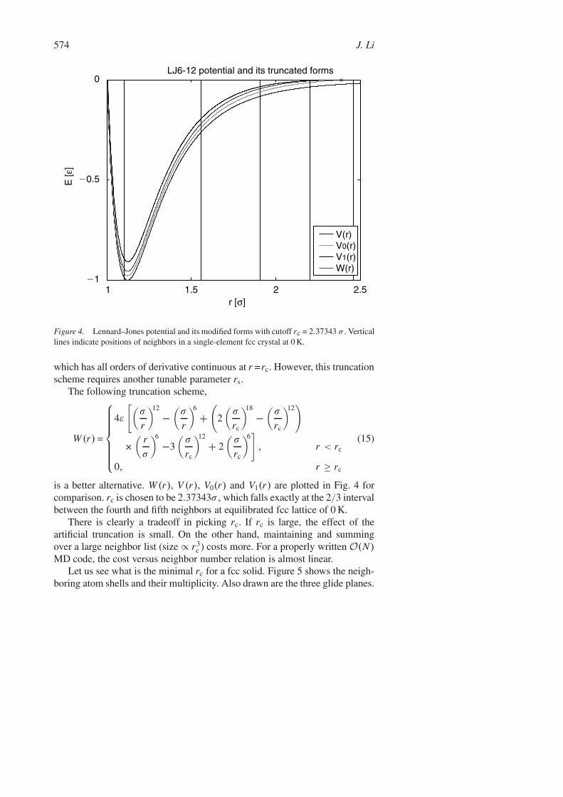
574 J. Li

1 1.5 2 2.5�1

�0.5

0

r [σ]

E [ε

]LJ6-12 potential and its truncated forms

V(r)V0(r)V1(r)W(r)

Figure 4. Lennard–Jones potential and its modified forms with cutoff rc = 2.37343 σ . Verticallines indicate positions of neighbors in a single-element fcc crystal at 0 K.

which has all orders of derivative continuous at r =rc. However, this truncationscheme requires another tunable parameter rs.

The following truncation scheme,

W (r) =

4ε

[(σ

r

)12

−(

σ

r

)6

+(

2(

σ

rc

)18

−(

σ

rc

)12)

×(

r

σ

)6

−3(

σ

rc

)12

+ 2(

σ

rc

)6]

, r < rc

0, r ≥ rc

(15)

is a better alternative. W (r), V (r), V0(r) and V1(r) are plotted in Fig. 4 forcomparison. rc is chosen to be 2.37343σ , which falls exactly at the 2/3 intervalbetween the fourth and fifth neighbors at equilibrated fcc lattice of 0 K.

There is clearly a tradeoff in picking rc. If rc is large, the effect of theartificial truncation is small. On the other hand, maintaining and summingover a large neighbor list (size ∝ r3

c ) costs more. For a properly written O(N)MD code, the cost versus neighbor number relation is almost linear.

Let us see what is the minimal rc for a fcc solid. Figure 5 shows the neigh-boring atom shells and their multiplicity. Also drawn are the three glide planes.

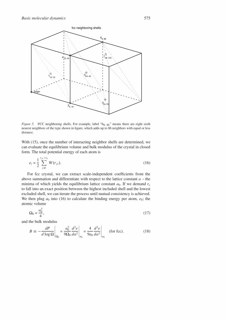
Basic molecular dynamics 575

748; 134

5

68; 86

fcc neighboring shells

324; 42

26; 18

4 12; 54

112; 12

origin

24; 78

Figure 5. FCC neighboring shells. For example, label “68; 86” means there are eight sixthnearest neighbors of the type shown in figure, which adds up to 86 neighbors with equal or lessdistance.

With (15), once the number of interacting neighbor shells are determined, wecan evaluate the equilibrium volume and bulk modulus of the crystal in closedform. The total potential energy of each atom is

ei =1

2

r j i <rc∑j=/i

W (r j i). (16)

For fcc crystal, we can extract scale-independent coefficients from theabove summation and differentiate with respect to the lattice constant a – theminima of which yields the equilibrium lattice constant a0. If we demand rc

to fall into an exact position between the highest included shell and the lowestexcluded shell, we can iterate the process until mutual consistency is achieved.We then plug a0 into (16) to calculate the binding energy per atom, e0; theatomic volume

�0 =a3

0

4, (17)

and the bulk modulus

B ≡ − dP

d log �

∣∣∣∣∣�0

=a2

0

9�0

d2e

da2

∣∣∣∣∣a0

=4

9a0

d2e

da2

∣∣∣∣∣a0

(for fcc). (18)

576 J. Li

Table 1. FCC neighboring shells included in Eq. (15) vs. properties

n N rc[σ ] a0[σ ] �0[σ 3] e0[ε] B[εσ−3]

1 12 1.44262944953 1.59871357076 1.02153204121 −2.03039845846 39.393601279022 18 1.81318453769 1.57691543349 0.98031403353 −4.95151157088 52.024485530613 42 2.11067974132 1.56224291246 0.95320365252 −6.12016548816 58.941487055804 54 2.37343077641 1.55584092331 0.94153307381 −6.84316556834 64.197386274685 78 2.61027143673 1.55211914976 0.93479241591 −7.27254778301 66.650939791626 86 2.82850677530 1.55023249772 0.93138774467 −7.55413237921 68.530933997657 134 3.03017270367 1.54842162594 0.92812761235 −7.74344974981 69.339617875728 140 3.21969263257 1.54727436382 0.92606612556 −7.88758411490 70.634521195779 176 3.39877500485 1.54643096926 0.92455259927 −7.99488847415 71.18713376234

10 200 3.56892997792 1.54577565469 0.92337773387 −8.07848627384 71.76659559499

The self-consistent results for rc ratio 2/3 are shown in Table 1. That is, rc

is exactly at 2/3 the distance between the nth interacting shell and the (n+1)thnon-interacting shell. The reason for 2/3(> 1/2) is that we expect thermalexpansion at finite temperature.

If one is after converged Lennard–Jones potential results, then rc = 4σ isrecommended. However, it is about five times more expensive per atom thanthe minimum-cutoff calculation with rc = 2.37343σ .

2. Integrators

An integrator advances the trajectory over small time increments �t :

x3N (t0) → x3N (t0 + �t) → x3N (t0 + 2�t) → · · · → x3N (t0 + L�t)

where L is usually ∼104 − 107. Here we give a brief overview of some pop-ular algorithms: central difference (Verlet, leap-frog, velocity Verlet, Beemanalgorithm) [1, 14], predictor-corrector [10], and symplectic integrators [8, 11].

2.1. Verlet Algorithm

Assuming x3N (t) trajectory is smooth, perform Taylor expansion

xi (t0 + �t) + xi (t0 − �t) = 2xi (t0) + xi (t0)(�t)2 + O((�t)4). (19)

Since xi (t0)= fi(t0)/mi can be evaluated given the atomic positions x3N (t0)at t = t0, x3N (t0 + �t) in turn may be approximated by,

xi (t0 + �t) = −xi (t0 − �t) + 2xi (t0) +(

fi (t0)

mi

)(�t)2 + O((�t)4).

(20)

Basic molecular dynamics 577

By throwing out the O((�t)4) term, we obtain a recursion formula to com-pute x3N (t0 + �t), x3N (t0 + 2�t), . . . successively, which is the Verlet [15]algorithm. The velocities do not participate in the recursion but are needed forproperty calculations. They can be approximated by

vi (t0) ≡ xi (t0) =1

2�t[xi (t0 + �t) − xi (t0 − �t)] + O((�t)2). (21)

To what degree does the outcome of the above recursion mimic the realtrajectory x3N (t)? Notice that in (20), assuming xi (t0) and xi (t0 −�t) areexact, and assuming we have a perfect computer with no machine error storingthe numbers or carrying out floating-point operations, the computed xi (t0+�t)would still be off from the real xi(t0 + �t) by O((�t)4), which is defined asthe local truncation error (LTE). LTE is an intrinsic error of the algorithm.Clearly, as �t → 0, LTE → 0, but that does not guarantee the algorithmworks, because what we want is x3N (t0 + t ′) for a given t ′, not xi (t0 + �t).To obtain x3N (t0 + t ′), we must integrate L = t ′/�t steps, and the differencebetween the computed x3N (t0 + t ′) and the real x3N (t0 + t ′) is called the globalerror. An algorithm can be useful only if when �t → 0, the global error → 0.Usually (but with exceptions), if LTE in position is ∼(�t)k+1, the global errorin position should be ∼(�t)k , in which case we call the algorithm a k-th ordermethod.

This is only half the story because the order of an algorithm only charac-terizes its performance when �t → 0. To save computational cost, most oftenone must adopt a quite large �t . Higher-order algorithms do not necessarilyperform better than lower-order algorithms at practical �t’s. In fact, they couldbe much worse by diverging spuriously (causing overflow and NaN), while amore robust method would just give a finite but manageable error for the same�t . This is the concept of the stability of a numerical algorithm. In linearODEs, the global error e of a certain normal mode k can always be written ase(ωk�t, T/�t) by dimensional analysis, where ωk is the mode’s angular fre-quency. One then can define the stability domain of an algorithm in the ω�tcomplex plane as the border where e(ωk�t, T/�t) starts to grow exponen-tially as a function of T/�t . To rephrase, a higher-order algorithm may have amuch smaller stability domain than the lower-order algorithm even though itse decays faster near the origin. Since e is usually larger for larger |ωk�t|, theoverall quality of an integration should be characterized by e(ωmax�t, T/�t)where ωmax is the maximum intrinsic frequency of the molecular dynamicssystem that we explicitly integrate. The main reason behind developing con-straint MD [1, 8] for some molecules is so that we do not have to integratetheir stiff intra-molecular vibrational modes, allowing one to take a larger �t ,so one can follow longer the “softer modes” that we are more interested in.This is also the rationale behind developing multiple time step integrators liker-RESPA [11].

578 J. Li

In addition to LTE, there is round-off error due to the computer’s finiteprecision. The effect of round-off error can be better understood in the stabilitydomain: (1) In most applications, the round-off error LTE, but it behaveslike white noise which has a very wide frequency spectrum, and so for thealgorithm to be stable at all, its stability domain must include the entire realω�t axis. However, as long as we ensure non-positive gain for all real ω�tmodes, the overall error should still be characterized by e(ωk�t, T/�t), sincethe white noise has negligible amplitude. (2) Some applications, especiallythose involving high-order algorithms, do push the machine precision limit. Inthose cases, equating LTE ∼ ε where ε is the machine’s relative accuracy,provides a practical lower bound to �t , since by reducing �t one can nolonger reduce (and indeed would increase) the global error. For single-precisionarithmetics (4 bytes to store one real number), ε ∼10−8; for double-precisionarithmetics (8 bytes to store one real number), ε ≈2.2 × 10−16; for quadruple-precision arithmetics (16 bytes to store one real number), ε ∼10−32.

2.2. Leap-frog Algorithm

Here we start out with v3N (t0 − �t/2) and x3N (t0), then,

vi

(t0 + �t

2

)= vi

(t0 − �t

2

)+(

fi (t0)

mi

)�t, (22)

followed by,

xi (t0 + �t) = xi (t0) + vi

(t0 + �t

2

)�t, (23)

and we have advanced by one step.The velocity at time t0 can be approximated by,

vi (t0) =1

2

[vi

(t0 − �t

2

)+ vi

(t0 + �t

2

)]+ O((�t)2). (24)

2.3. Velocity Verlet Algorithm

We start out with x3N (t0) and v3N (t0), then,

xi (t0 + �t) = xi (t0) + vi (t0)�t + 1

2

(fi (t0)

mi

)(�t)2, (25)

evaluate f3N (t0 + �t), and then,

vi (t0 + �t) = vi (t0) + 1

2

[fi(t0)

mi+ fi (t0 + �t)

mi

]�t, (26)

Basic molecular dynamics 579

and we have advanced by one step. Since we can have x3N (t0) and v3N (t0)simultaneously, it is popular.

2.4. Beeman Algorithm

It is similar to the velocity Verlet algorithm. We start out with x3N (t0),f3N (t0 − �t), f3N (t0) and v3N (t0), then,

xi (t0 + �t) = xi (t0) + vi (t0)�t +[

4fi (t0) − fi (t0 − �t)

mi

](�t)2

6, (27)

evaluate f3N (t0 + �t), and then,

vi (t0 + �t) = vi (t0) +[

2fi (t0 + �t) + 5fi (t0) − fi (t0 − �t)

mi

]�t

6, (28)

and we have advanced by one step. Note that just like the leap-frog and veloc-ity Verlet algorithms, the Beeman algorithm gives identical trajectory as theVerlet algorithm [1,14] in the absence of machine error, with 4th-order LTEin position. However, it gives better velocity estimate (3rd-order LTE) thanthe leap-frog or velocity Verlet (2nd-order LTE). The best velocity estimate(4th-order LTE) can be achieved by the so-called velocity-corrected Verletalgorithm [14], but it requires knowing the next two steps’ positions.

2.5. Predictor-corrector Algorithm

Let us take the often used 6-value predictor-corrector algorithm [10] asan example. We start out with 6 × 3N storage: x3N(0)(t0), x3N(1)(t0), x3N(2)

(t0), . . . , x3N(5)(t0), where x3N(k)(t) is defined by,

x(k)i (t) ≡

(dkx(t)

i

dtk

)((�t)k

k!

). (29)

The iteration consists of prediction, evaluation, and correction steps:

2.5.1. Prediction step

x(0)i = x(0)

i + x(1)i + x(2)

i + x(3)i + x(4)

i + x(5)i ,

x(1)i = x(1)

i + 2x(2)i + 3x(3)

i + 4x(4)i + 5x(5)

i ,

x(2)i = x(2)

i + 3x(3)i + 6x(4)

i + 10x(5)i ,

x(3)i = x(3)

i + 4x(4)i + 10x(5)

i ,

x(4)i = x(4)

i + 5x(5)i . (30)

580 J. Li

The general formula for the above is

x(k)i =

M−1∑k′=k

[k ′!

(k ′ − k)!k!

]x(k′)

i , k = 0, . . . , M − 2, (31)

with M = 6 here. The evaluation must proceed from 0 to M − 2 sequentially.

2.5.2. Evaluation step

Evaluate force f3N using the newly obtained x3N(0).

2.5.3. Correction step

Define the error e3N as,

ei ≡ x(2)i −

(fi

mi

)((�t)2

2!

). (32)

Then apply corrections,

x(k)i = x(k)

i − CMkei , k = 0, . . . , M − 1, (33)

where CMk are constants listed in Table 2.It is clear that the LTE for x3N is O((�t)M) after the prediction step. But

one can show that the LTE is reduced to O((�t)M+1) after the correction stepif f3N depends on x3N only, and not on the velocity. And so the global errorwould be O((�t)M).

2.6. Symplectic Integrators

In the absence of round-off error, certain numerical integrators rigorouslymaintain the phase-space volume conservation property (Liouville’s theorem)of Hamiltonian dynamics, which are then called symplectic integrators. This

Table 2. Gear predictor-corrector coefficients

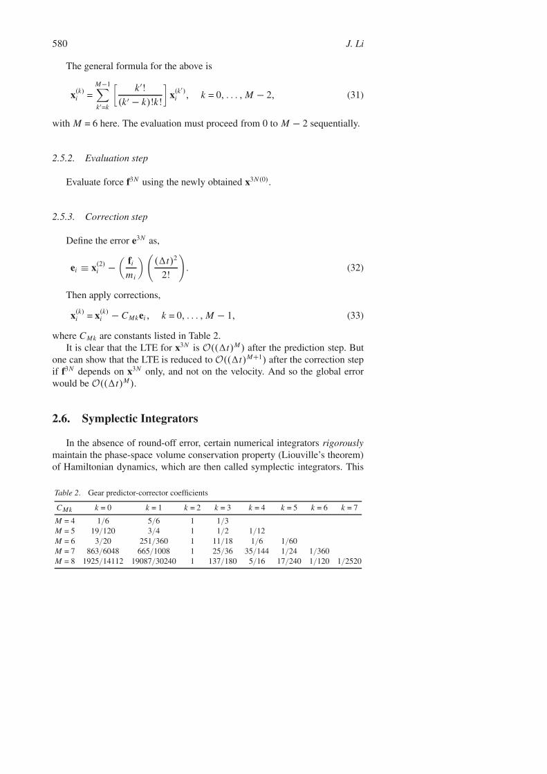
CMk k = 0 k = 1 k = 2 k = 3 k = 4 k = 5 k = 6 k = 7

M = 4 1/6 5/6 1 1/3M = 5 19/120 3/4 1 1/2 1/12M = 6 3/20 251/360 1 11/18 1/6 1/60M = 7 863/6048 665/1008 1 25/36 35/144 1/24 1/360M = 8 1925/14112 19087/30240 1 137/180 5/16 17/240 1/120 1/2520

Basic molecular dynamics 581

100 150 200 300 400 500 600 700 800 900 100010

�6

10�5

10�4

10�3

10�2

10�1

100

number of force evaluations per period

Integration of 100 periods of Kepler orbitals with eccentricity 0.5

Ruth83Schlier98_6aTsitouras99Calvo93Schlier00_6bSchlier00_8c4th Runge-Kutta4th Gear5th Gear6th Gear7th Gear8th Gear

150 200 300 400 500 600 700 800 900 1000 1200 1400 16001800 200010

�8

10�7

10�6

10�5

10�4

10�3

10�2

10�1

100

number of force evaluations per period

Integration of 1000 periods of Kepler orbitals with eccentricity 0.5

Ruth83Schlier98_6aTsitouras99Calvo93Schlier00_6bSchlier00_8c4th Runge-Kutta4th Gear5th Gear6th Gear7th Gear8th Gear

II fin

al (

p,q)

err

or II

2

II fin

al (

p,q)

err

or II

2

Figure 6. (a) Phase error after integrating 100 periods of Kepler orbitals. (b) Phase error afterintegrating 1000 periods of Kepler orbitals.

property severely limits the possibilities of mapping from initial to final states,and for this reason symplectic integrators tend to have much better total energyconservation in the long run. The velocity Verlet algorithm is in fact symplec-tic, followed by higher-order extensions [16, 17].

We have benchmarked the two families of integrators (Fig. 6) by numeri-cally solving the two-body Kepler’s problem (eccentricity 0.5) which is non-linear and periodic, and comparing with the exact analytical solution. The twofamilies have different global error versus time characteristics: non-symplecticintegrators tend to have linear energy error (�E ∝ t) and quadratic phase error(|��| ∝ t2), while symplectic integrators tend to have constant (fluctuating)energy error (�E ∝ t0) and linear phase error (|��|∝ t), with respect to time.Therefore the long-term performance of a symplectic tends to be asymptoti-cally superior to that of a non-symplectic integrator. But, it is found that for areasonable integration duration, say 100 Kepler periods, high-order predictor-corrector integrators can have a better performance than the best of the currentsymplectic integrators at large integration timestep (small number of forceevaluations per period). This is important, because it means that in a realcondensed-matter system if one does not care about the correlation of a modebeyond 100 oscillation periods, then high-order predictor-corrector algorithmscan achieve the desired accuracy at a lower computational cost.

3. Order-N MD Simulation With Short-RangePotential

We outline here a linked-bin algorithm that allows one to perform MDsimulation in a PBC supercell with O(N) computational effort per timestep,where N is the number of atoms in the supercell (Fig. 7). Such approach

582 J. Li

each timestep: N

?

(a)

?

1 2 3

(b)

rc

2D usage ratio: 35%

3D usage ratio: 16% (!)

(c)2

Figure 7. There are N atoms in the supercell. (a) The circle around a particular atom withradius rc indicates the range of its interaction with other atoms. (b) The supercell is dividedinto a number of bins, which have dimensions such that an atom can only possibly interactwith atoms in adjacent 27 bins in 3D (9 in 2D). (c) This shows that an atom–atom list is stillnecessary because on average there are only 16% of the atoms in 3D in adjacent bins thatinteract with the particular atom.

is found to outperform the brute-force Verlet neighbor-list update algorithm,which is O(N2), when N exceeds a few thousand atoms. The algorithm to beintroduced here allows for arbitrary supercell deformation during a simulation,and is implemented in large-scale MD and conjugate gradient relaxationprograms as well as a visualization program [3].

Denote the three edges of a supercell in Cartesian frame by row vectors h1,h2, h3, which stack together to form a 3 × 3 matrix H. The inverse of the Hmatrix B ≡ H−1 satisfies

I = HB = BH. (34)

If we define row vectors

b1 ≡ (B11, B21, B31), b2 ≡ (B12, B22, B32), b3 ≡ (B13, B23, B33),

(35)

then (34) is equivalent to

hi · b j ≡ hibTj = δi j . (36)

Since b1 is perpendicular to both h2 and h3, it must be collinear with thenormal direction n of the plane spanned by h2 and h3 : b1 ≡ |b1|n. And soby (36),

1 = h1 · b1 = h1 · (|b1|n) = |b1|(h1 · n). (37)

Basic molecular dynamics 583

But |h1 · n| is nothing other than the thickness of the supercell along the h1

edge. Therefore, the thicknesses (distances between two parallel surfaces) ofthe supercell are,

d1 =1

|b1| , d2 =1

|b2| , d3 =1

|b3| . (38)

The position of atom i is specified by a row vector, si = (si1, si2, si3), withsiµ satisfying

0 ≤ siµ < 1, µ = 1, . . . , 3, (39)

and the Cartesian coordinate of this atom, xi , also a row vector, is

xi = si1h1 + si2h2 + si3h3 = si H, (40)

where siµ has the geometrical interpretation of the fraction of the µth edgein order to construct xi . We will simulate particle systems that interact viashort-range potentials of cutoff radius rc (see previous section for potentialtruncation schemes). In the case of multi-component system, rc is generalizedto a matrix rαβ

c , where α ≡ c(i), β ≡ c( j) are the chemical types of atomi and j , respectively. We then define

x j i ≡ x j − xi , r j i ≡ |x j i |, x j i ≡ x j i

r j i. (41)

The design of the program should allow for arbitrary changes in H thatinclude strain and rotational components (see Chap. 2.19). One should usethe Lagrangian strain η, a true rank-2 tensor under coordinate frame transfor-mation, to measure the deformation of a supercell. To define η, one needs areference H0 of a previous time, with x0 = sH0 and dx0 = (ds)H0, and imaginethat with s fixed, dx0 is transformed to dx = (ds)H, under H0 → H ≡ H0J.

The Lagrangian strain is defined by the change in the differential linelength,

dl2 = dx dxT ≡ dx0(I + 2η)dxT0 , (42)

where by plugging in dx = (ds)H = (dx0)H−10 H = (dx0)J, η is seen to be

η = 12

(H−1

0 HHT H−T0 − I

)= 1

2

(JJT − I

). (43)

Because η is a symmetric matrix, it always has three mutually orthogo-nal eigen-directions x1η = x1η1, x2η = x2η2, x3η = x3η3. Along those direc-tions, the line lengths are changed by factors

√1 + 2η1,

√1 + 2η2,

√1 + 2η3,

which achieve extrema among all line directions. Thus, as long as η1, η2 and η3

oscillate between [−ηbound, ηbound] for some chosen ηbound, any line segment atH0 can be scaled by no more than

√1 + 2ηbound and no less than

√1 − 2ηbound.

That is, if we define length measure

L(�s, H) ≡ √�sHHT �sT , (44)

584 J. Li

then so long as η1, η2, η3 oscillate between [ηmin, ηmax], there is√1 + 2ηmin L(�s, H0) ≤ L(�s, H) ≤ √

1 + 2ηmax L(�s, H0). (45)

One can use the above result to define a strain session, which begins withH0 = H and during which no line segment is allowed to shrink by less than athreshold fc ≤ 1, compared to its length at H0. This is equivalent to requiringthat,

f ≡ √1 + 2 (min(η1, η2, η3)) ≤ fc. (46)

Whenever the above condition is violated, the session terminates and a newsession starts with the present H as the new H0, and triggers a repartitioningof the supercell into equally-sized bins, which is called a strain-induced binrepartitioning.

The purpose of bin partition (see Fig. 7) is the following: it can be a verydemanding task to determine if atoms i , j are within rc or not, for all possiblei j combinations. Formally, this requires checking

r j i ≡ L(�s j i , H) ≤ rc. (47)

Because si , s j and H are in general all moving – they differ from step tostep, it appears that we have to check this at each step. This would indeed bethe case but for the observation that, in most MD, MC and static minimizationprocedures, si ’s of most atoms and H often change only slightly from the pre-vious step. Therefore, once we ensured that (47) held at some previous step,we can devise a sufficient condition to test if (47) still must hold now, at a muchsmaller cost. Only when this sufficient condition breaks down do we resort toa more complicated search and check in the fashion of (47).

As a side note, it is often more efficient to count interaction pairs if thepotential function allows for easy use of such half-lists, such as pair- or EAMpotentials, which achieves 50% saving in memory. In these scenarios we pick aunique “host” atom among i and j to store the information about thei j -pair, that is, a particle’s list only keeps possible pairs that are under itsown care. For load-balancing it is best if the responsibilities are distributedevenly among particles. We use a pseudo-random choice of: if i + j is oddand i > j , or if i + j is even and i < j , then i is the host; otherwise it is j .As i > j is “uncorrelated” with whether i + j is even or odd, significant loadimbalance is unlikely to occur even if the indices correlate strongly with theatoms’ positions.

The step-to-step small change is exploited as follows: one associates eachsi with a semi-mobile reduced coordinate sa

i called atom i’s anchor (Fig. 8).At each step, one checks if L(si − sa

i , H), that is, the current distance betweeni and its anchor, is greater than a certain rdrift ≥ r0

drift or not. If it is not, then sai

does not change; if it is, then one redefines sai ≡ si at this step, which is called

Basic molecular dynamics 585

L

d = 0.05rc

d

d

Usually,

atom trajectory

anchor trajectory

Figure 8. This illustrates the concepts of an anchor, which is the relative immbobile part ofan atom’s trajectory. Using an anchor–anchor list, we can derive a “flash” condition that locallyupdates an atom’s neighbor-list when the atom drifts sufficiently far away from its anchor.

atom i’s flash incident. At atom i’s flash, it is required to update records of allatoms (part of the records may be stored in j ’s list, if 50%-saving is used andj happens to be the host of the i j pair) whose anchors satisfy

L(saj − sa

i , H0) ≤ rlist ≡ rc + 2r0drift

fc. (48)

Note that the distance is between anchors instead of atoms (sai = si , though),

and the length is measured by H0, not the current H. (48) nominally takesO(N) work per flash, but we may reduce it to O(1) work per flash by parti-tioning the supercell into m1 × m2 × m3 bins at the start of the session, whosethicknesses by H0 (see (38)) are required to be greater than or equal to rlist:

d1(H0)

m1,

d2(H0)

m2,

d3(H0)

m3≥ rlist. (49)

The bins deform with H and remains commensurate with it, that is, itss-width 1/m1, 1/m2, 1/m3 remains fixed during a strain session. Each binkeeps an updated list of all anchors inside. When atom i flashes, it also updatesthe bin-anchor list if necessary. Then, if at the time of i’s flash two anchors areseparated by more than one bin, there would be

L(saj − sa

i , H0) >d1(H0)

m1,

d2(H0)

m2,

d3(H0)

m3≥ rlist, (50)

and they cannot possibly satisfy (48). Therefore we only need to test (48) foranchors within adjacent 27 bins. To synchronize, all atoms flash at the start of astrain session. From then on, atoms flash individually whenever L(si−sa

i , H)>rdrift. If two anchors flash at the same step in a loop, the first flash may get itwrong – that is, missing the second anchor, but the second flash will correctthe mistake. The important thing here is not to lose an interaction. We seethat to maintain anchor lists that captures all solutions to (48) among the latestanchors, it takes only O(N) work per step, and the pre-factor of which is alsosmall because flash events happen quite infrequently for a tolerably large r0

drift.

586 J. Li

The central claim of the scheme is that if j is not in i’s anchor records(suppose i’s last flash is more recent than j ’s), which was created some timeago in the strain session, then r j i > rc. The reason is that the current separationbetween the anchor i and anchor j , L(sa

j − sai , H), is greater than rc + 2r0

drift,since by (45), (46) and (48),

L(saj − sa

i , H)≥ f · L(saj − sa

i , H0)> f · rlist ≥ fc · rlist = fc · rc + 2r0drift

fc.

(51)

So we see that r j i > rc maintains if neither i or j currently drifts more than

rdrift ≡ f · rlist − rc

2≥ r0

drift, (52)

from respective anchors. Put it another way, when we design rlist in (48), wetake into consideration both atom drifts and H shrinkage which both may bringi j closer than rc, but since the current H shrinkage has not yet reached thedesigned critical value, we can convert it to more leeway for the atom drifts.

For multi-component systems, we define

rαβlist ≡ rαβ

c + 2r0drift

fc, (53)

where both fc and r0drift are species-independent constants, and r0

drift can bethought of as putting a lower bound on rdrift, so flash events cannot occur toofrequently. At each bin repartitioning, we would require

d1(H0)

m1,

d2(H0)

m2,

d3(H0)

m3≥ max

α,βrαβ

list. (54)

And during the strain session, f ≥ fc, we have

rαdrift ≡ min

[min

β

(f · rαβ

list − rαβc

2

), min

β

(f · rβα

list − rβαc

2

)], (55)

a time- and species-dependent atom drift bound that controls whether an atomof species α needs to flash.

4. Molecular Dynamics Codes

At present there are several high-quality molecular dynamics programs inthe public domain, such as LAMMPS [18], DL POLY [19, 20], Moldy [21],IMD [22, 23], and some codes with biomolecular focus, such as NAMD [24,25] and Gromacs [26, 27]. CHARMM [28] and AMBER [29] are not free butare standard and extremely powerful codes in biology.

Basic molecular dynamics 587

References

[1] M. Allen and D. Tildesley, Computer Simulation of Liquids, Clarendon Press, NewYork, 1987.

[2] J. Li, L. Porter, and S. Yip, “Atomistic modeling of finite-temperature properties ofcrystalline beta-SiC - II. Thermal conductivity and effects of point defects,” J. Nucl.Mater., 255, 139–152, 1998.

[3] J. Li, “AtomEye: an efficient atomistic configuration viewer,” Model. Simul. Mater.Sci. Eng., 11, 173–177, 2003.

[4] D. Chandler, Introduction to Modern Statistical Mechanics, Oxford University Press,New York, 1987.

[5] M. Born and K. Huang, Dynamical Theory of Crystal Lattices, 2nd edn., ClarendonPress, Oxford, 1954.

[6] R. Parr and W. Yang, Density-functional Theory of Atoms and Molecules, ClarendonPress, Oxford, 1989.

[7] S.D. Ivanov, A.P. Lyubartsev, and A. Laaksonen, “Bead-Fourier path integral molec-ular dynamics,” Phys. Rev. E, 67, art. no.–066710, 2003.

[8] T. Schlick, Molecular Modeling and Simulation, Springer, Berlin, 2002.[9] W. Press, B. Flannery, S. Teukolsky, and W. Vetterling, Numerical Recipes in C:

the Art of Scientific Computing, 2nd edn., Cambridge University Press, Cambridge,1992.

[10] C. Gear, Numerical Initial Value Problems in Ordinary Differential Equation,Prentice-Hall, Englewood Cliffs, NJ, 1971.

[11] M.E. Tuckerman and G.J. Martyna, “Understanding modern molecular dynamics:techniques and applications,” J. Phys. Chem. B, 104, 159–178, 2000.

[12] S. Nose, “A unified formulation of the constant temperature molecular dynamicsmethods,” J. Chem. Phys., 81, 511–519, 1984.

[13] W.G. Hoover, “Canonical dynamics – equilibrium phase-space distributions,” Phys.Rev. A, 31, 1695–1697, 1985.

[14] D. Frenkel and B. Smit, “Understanding molecular simulation: from algorithms toapplications,” 2nd ed., Academic Press, San Diego, 2002.

[15] L. Verlet, “Computer “experiments” on classical fluids. I. Thermodynamical proper-ties of Lennard–Jones molecules,” Phys. Rev., 159, 98–103, 1967.

[16] H. Yoshida, “Construction of higher-order symplectic integrators,” Phys. Lett. A, 150,262–268, 1990.

[17] J. Sanz-Serna and M. Calvo, Numerical Hamiltonian Problems, Chapman & Hall,London, 1994.

[18] S. Plimpton, “Fast parallel algorithms for short-range molecular-dynamics,” J. Com-put. Phys., 117, 1–19, 1995.

[19] W. Smith and T.R. Forester, “DL POLY 2.0: a general-purpose parallel moleculardynamics simulation package,” J. Mol. Graph., 14, 136–141, 1996.

[20] W. Smith, C.W. Yong, and P.M. Rodger, “DL POLY: application to molecular simu-lation,” Mol. Simul., 28, 385–471, 2002.

[21] K. Refson, “Moldy: a portable molecular dynamics simulation program for serialand parallel computers,” Comput. Phys. Commun., 126, 310–329, 2000.

[22] J. Stadler, R. Mikulla, and H.-R. Trebin, “IMD: A Software Package for Molecu-lar Dynamics Studies on Parallel Computers,” Int. J. Mod. Phys. C, 8, 1131–1140,1997.

[23] J. Roth, F. Gahler, and H.-R. Trebin, “A molecular dynamics run with 5,180,116,000particles,” Int. J. Mod. Phys. C, 11, 317–322, 2000.

588 J. Li

[24] M.T. Nelson, W. Humphrey, A. Gursoy, A. Dalke, L.V. Kale, R.D. Skeel, andK. Schulten, “NAMD: a parallel, object oriented molecular dynamics program,” Int.J. Supercomput. Appl. High Perform. Comput., 10, 251–268, 1996.

[25] L. Kale, R. Skeel, M. Bhandarkar, R. Brunner, A. Gursoy, N. Krawetz, J. Phillips,A. Shinozaki, K. Varadarajan, and K. Schulten, “NAMD2: Greater scalability forparallel molecular dynamics,” J. Comput. Phys., 151, 283–312, 1999.

[26] H.J.C. Berendsen, D. Vanderspoel, and R. Vandrunen, “Gromacs – a message-passing parallel molecular-dynamics implementation,” Comput. Phys. Commun., 91,43–56, 1995.

[27] E. Lindahl, B. Hess, and D. van der Spoel, “GROMACS 3.0: a package for molecularsimulation and trajectory analysis,” J. Mol. Model., 7, 306–317, 2001.

[28] B.R. Brooks, R.E. Bruccoleri, B.D. Olafson, D.J. States, S. Swaminathan, andM. Karplus, “Charmm – a program for macromolecular energy, minimization, anddynamics calculations,” J. Comput. Chem., 4, 187–217, 1983.

[29] D.A. Pearlman, D.A. Case, J.W. Caldwell, W.S. Ross, T.E. Cheatham, S. Debolt,D. Ferguson, G. Seibel, and P. Kollman, “Amber, a package of computer-programsfor applying molecular mechanics, normal-mode analysis, molecular-dynamicsand freeenergy calculations to simulate the structural and energetic properties ofmolecules,” Comput. Phys. Commun., 91, 1–41, 1995.