2017 Eye on the Market Outlook Special Topics - J.P. Morgan · 2017 Eye on the Market Outlook...

EYE ON THE MARKET • MICHAEL CEMBALEST • OUTLOOK 2017 JANUARY 1, 2017

26

EYE ON THE MARKET MICHAEL CEMBALEST OUTLOOK 2017 JANUARY 1, 2017

26

2017 Eye on the Market Outlook Special Topics

1 Leverage What amount of leverage can survive a world of volatile markets? Now that the window for low-cost borrowing may be closing, we look at history and the future

2 Active management

The end of “peak central bank intervention” may reduce distortions and help active managers

Page 29

3 LNG Rising US natural gas prices due to large-scale US LNG exports? Unlikely on both counts. What Dep’t of Energy LNG export approvals mean, and what they don’t

Page 31

4 Tax efficient investing

How to simultaneously employ tax loss harvesting and generate market returns

Page 33

5 Infrastructure The role for public-private partnerships: PPPs have their critics, but the Obama administration is not among them. When should investors participate?

Page 34

6 Clean coal/CCS The biggest problem with “clean coal”: scope. Infrastructure required to make carbon capture and storage a meaningful contributor is vastly underestimated

Page 36

7 Internet-based business models

How helpful have user growth metrics been in assessing new internet-based business models? Not very

Page 37

8 Commodity prices Markets are looking past inventory gluts given huge declines in capex; remembering the commodity surge of the 1970s and Richard Nixon

Page 38

Chapter links

Brief videos of Michael discussing each of these special topics are available on the True Believers webpage.

Page 27

http://am.jpmorgan.com/private-bank/public/gl/en/eotm-outlook-2017#specialtopics


27


27

[1] What amount of portfolio leverage can survive a world of volatile markets?

In our study of state pension plans, we found that median expected long-term returns on plan assets were around 7.5%. While corporate plans discount liabilities at lower rates than state plans, Milliman cites a funding ratio of 76% for the 100 largest corporate plans, indicating that many may need higher returns. As a result, some pensions, endowments, foundations and individuals have contemplated leverage (in one form or another) to increase portfolio returns. Since the window of opportunity to borrow at historically low levels may be closing, we wanted to take a closer look at leverage this year.

How much leverage can a portfolio sustain in a world of volatile markets, particularly since correlations among asset classes can rise close to 1.0 during a crisis? For purposes of this analysis, we define successful use of leverage as a scenario in which a portfolio does not experience “failure” over a 10-year period. We also assume that leverage is implemented through long-term fixed rate borrowing, and that leverage proceeds are used to gross up existing portfolio holdings on a pro-rata basis.

We looked at leverage from two perspectives: historical, and forward-looking. Our definitions of failure differ in each approach. The goal: develop some rough estimates of how much leverage a portfolio could carry without causing regret and recriminations at some point down the road.

The empirical, historical analysis

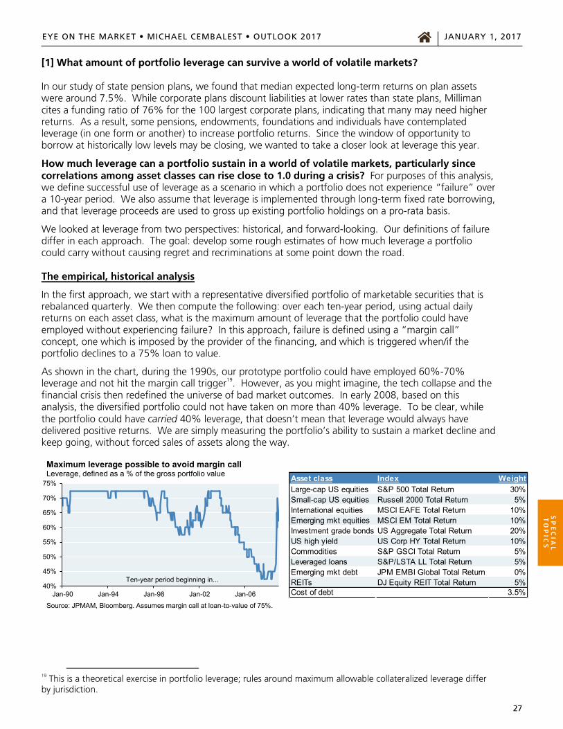
In the first approach, we start with a representative diversified portfolio of marketable securities that is rebalanced quarterly. We then compute the following: over each ten-year period, using actual daily returns on each asset class, what is the maximum amount of leverage that the portfolio could have employed without experiencing failure? In this approach, failure is defined using a “margin call” concept, one which is imposed by the provider of the financing, and which is triggered when/if the portfolio declines to a 75% loan to value.

As shown in the chart, during the 1990s, our prototype portfolio could have employed 60%-70% leverage and not hit the margin call trigger19. However, as you might imagine, the tech collapse and the financial crisis then redefined the universe of bad market outcomes. In early 2008, based on this analysis, the diversified portfolio could not have taken on more than 40% leverage. To be clear, while the portfolio could have carried 40% leverage, that doesn’t mean that leverage would always have delivered positive returns. We are simply measuring the portfolio’s ability to sustain a market decline and keep going, without forced sales of assets along the way.

19 This is a theoretical exercise in portfolio leverage; rules around maximum allowable collateralized leverage differ by jurisdiction.

40%

45%

50%

55%

60%

65%

70%

75%

Jan-90 Jan-94 Jan-98 Jan-02 Jan-06

Source: JPMAM, Bloomberg. Assumes margin call at loan-to-value of 75%.

Maximum leverage possible to avoid margin callLeverage, defined as a % of the gross portfolio value

Ten-year period beginning in...

Asset class Index WeightLarge-cap US equities S&P 500 Total Return 30%Small-cap US equities Russell 2000 Total Return 5%International equities MSCI EAFE Total Return 10%Emerging mkt equities MSCI EM Total Return 10%Investment grade bonds US Aggregate Total Return 20%US high yield US Corp HY Total Return 10%Commodities S&P GSCI Total Return 5%Leveraged loans S&P/LSTA LL Total Return 5%Emerging mkt debt JPM EMBI Global Total Return 0%REITs DJ Equity REIT Total Return 5%Cost of debt 3.5%

SP

EC

IAL

TO

PIC

S


28


28

Asset class WeightGlobal equities 40%US investment grade bonds 30%US high yield bonds 5%Diversified hedge funds 5%US private equity 5%Commodities 5%US real estate 10%Cash 0%Cost of debt 3.5%

Should the universe of bad market outcomes forever be impacted by the implosion in 2008, given increases in bank capitalization, the reduction in the shadow banking system, the migration of certain derivative contracts to centralized exchanges, the decline in non-conforming mortgages, etc? That is something that every portfolio manager, risk manager, chief investment officer and investor has to grapple with. If your answer is “yes”, then leverage of 40% would be as high as you would go based on the historical analysis. The forward-looking analysis

In this approach, future returns are based on J.P. Morgan’s Long-Term Capital Markets Assumptions, and are subject to various “non-normal” and “fat left tail” shocks20. In this approach, financing is assumed to be non-recourse. As a result, failure is effectively defined by the CIO, who would have to decide if it was a good or bad idea in hindsight to have used leverage. This is obviously a subjective question, but we can try to put some parameters around it. We define failure as follows: when the portfolio’s value falls to the point where, given the time remaining and our expected returns, it would be very unlikely to earn its way back21.

The chart below shows the rising probability of failure at different levels of leverage. The bar is higher here since, unlike the prior analysis which simply has to avoid a margin call, this portfolio needs to generate a return at least equal to the cost of its leverage over the entire horizon. That’s one reason why the failure rate is never zero. Looking again at the 40% leverage case, is an incremental 15% failure rate “too high”? That’s a subjective determination that has to be considered against the consequences of unlevered portfolio returns that are below target levels, the ability to restructure pension obligations if needed, and the ability of the plan and/or its workers to make emergency contributions. Our Multi-Asset Solutions Quantitative Research and Strategies group looks closely at these questions on behalf of our institutional clients, and can go into greater detail regarding the calculations and assumptions used in this part of the analysis.

20 For more information on modeling such scenarios, see “Non-Normality of Market Returns: A Framework for Asset Allocation Decision-Making”, Abdullah Sheikh, J.P. Morgan Asset Management. 21 In each scenario, we assume a target return of at least the cost of the debt on the entire portfolio over the 10-year window. We then assume failure occurs when the investor has less than a 20% chance of achieving the stated goal based on the portfolio’s value at that point and future expected returns.

0%

5%

10%

15%

20%

25%

30%

35%

10% 20% 30% 40% 50% 60% 70%Leverage, as a % of gross portfolio value

Source: J.P. Morgan Asset Management. December 2016.

Failure rate as a function of leverageChange in failure rate vs. 0% leverage baseline

SP

EC

IAL

T

OP

ICS


29


29

[2] Prospects for improved active equity management performance The last few years have been difficult for some large-cap US active equity managers. In my view, this outcome is partially explained by distortions resulting from the most extreme monetary policy experiment in history. Now that markets are beginning to price in gradual exits from these policies, prospects for active equity management may improve.

While it’s hard to generalize, the typical large-cap US active equity manager employs many of the following approaches:

Prefers low P/E stocks to high P/E stocks

Prefers to equal-weight portfolios rather than market-cap weight them

Underweights high-dividend, low-volatility stocks such as consumer staples, REITs, telecom and utilities (the “bond proxy” stocks)

Does not prefer stocks simply based on their positive price momentum

Holds some cash rather than being fully invested

Often has an out-of-index position in European, Asian or US mid-cap stocks

Prefers stocks with high degrees of idiosyncratic risk (i.e., stocks whose returns are not easily explained as a function of other factors)

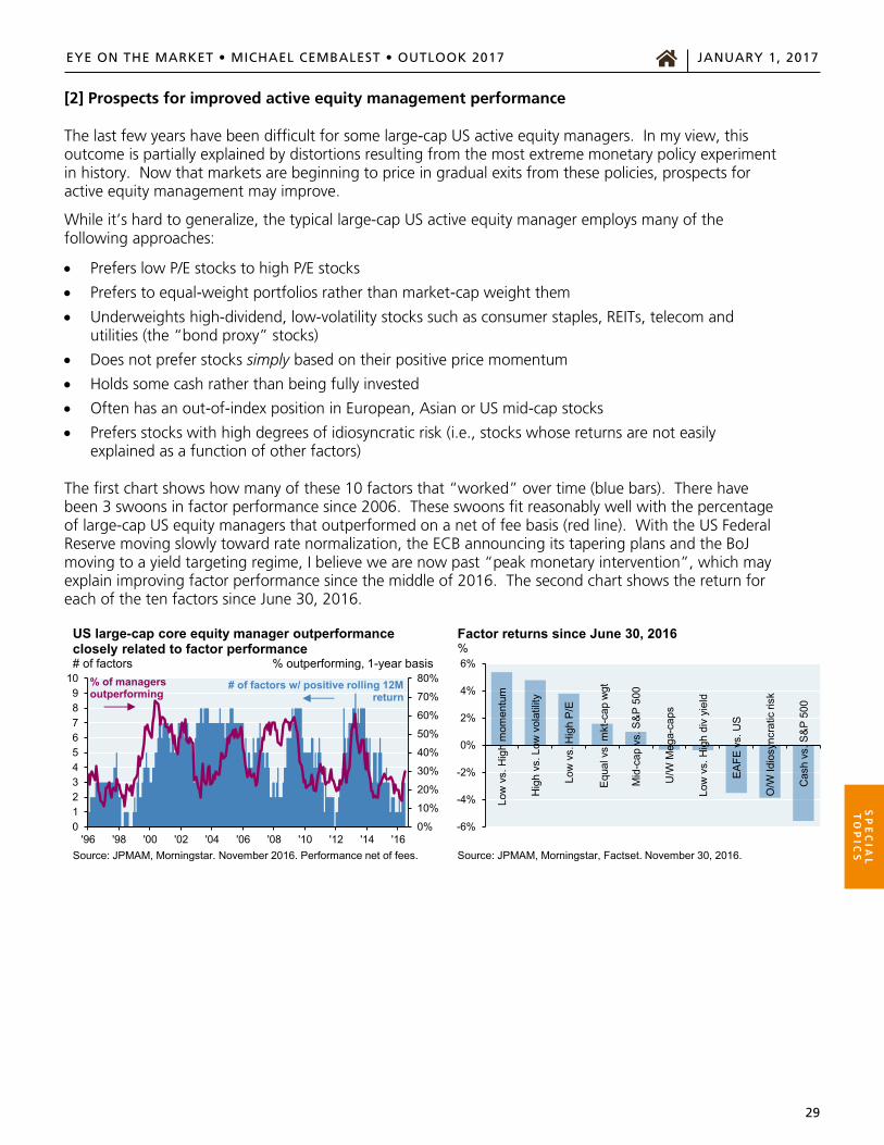
The first chart shows how many of these 10 factors that “worked” over time (blue bars). There have been 3 swoons in factor performance since 2006. These swoons fit reasonably well with the percentage of large-cap US equity managers that outperformed on a net of fee basis (red line). With the US Federal Reserve moving slowly toward rate normalization, the ECB announcing its tapering plans and the BoJ moving to a yield targeting regime, I believe we are now past “peak monetary intervention”, which may explain improving factor performance since the middle of 2016. The second chart shows the return for each of the ten factors since June 30, 2016.

0%

10%

20%

30%

40%

50%

60%

70%

80%

0123456789

10

'96 '98 '00 '02 '04 '06 '08 '10 '12 '14 '16Source: JPMAM, Morningstar. November 2016. Performance net of fees.

US large-cap core equity manager outperformance closely related to factor performance# of factors % outperforming, 1-year basis

# of factors w/ positive rolling 12M return

% of managers outperforming

Low

vs.

Hig

h m

omen

tum

Hig

h vs

. Low

vol

atili

ty

Low

vs.

Hig

h P

/E

Equ

al v

s. m

kt-c

ap w

gt

Mid

-cap

vs.

S&

P 5

00

U/W

Meg

a-ca

ps

Low

vs.

Hig

h di

v yi

eld

EA

FE v

s. U

S

O/W

Idio

sync

ratic

risk

Cas

h vs

. S&

P 5

00

-6%

-4%

-2%

0%

2%

4%

6%

Source: JPMAM, Morningstar, Factset. November 30, 2016.

Factor returns since June 30, 2016%

SP

EC

IAL

T

OP

ICS


30


30

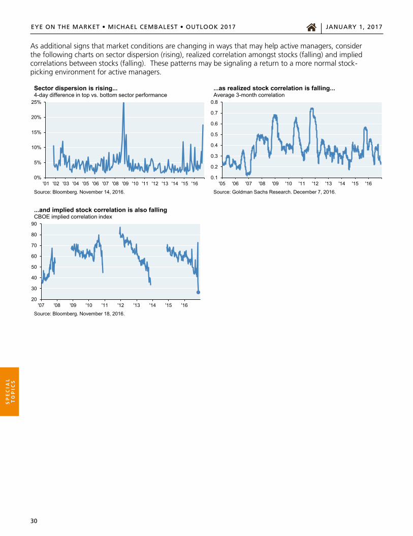
As additional signs that market conditions are changing in ways that may help active managers, consider the following charts on sector dispersion (rising), realized correlation amongst stocks (falling) and implied correlations between stocks (falling). These patterns may be signaling a return to a more normal stock-picking environment for active managers.

0%

5%

10%

15%

20%

25%

'01 '02 '03 '04 '05 '06 '07 '08 '09 '10 '11 '12 '13 '14 '15 '16

Hun

dred

s

Source: Bloomberg. November 14, 2016.

Sector dispersion is rising...4-day difference in top vs. bottom sector performance

0.1

0.2

0.3

0.4

0.5

0.6

0.7

0.8

'05 '06 '07 '08 '09 '10 '11 '12 '13 '14 '15 '16

Source: Goldman Sachs Research. December 7, 2016.

...as realized stock correlation is falling...Average 3-month correlation

20

30

40

50

60

70

80

90

'07 '08 '09 '10 '11 '12 '13 '14 '15 '16

Source: Bloomberg. November 18, 2016.

...and implied stock correlation is also fallingCBOE implied correlation index

SP

EC

IAL

T

OP

ICS


31


31

[3] Rising US natural gas prices due to large-scale US LNG exports? Unlikely on both counts I was reading reports that mentioned how the US Department of Energy has approved applications for US firms to export 50 billion cubic feet per day of liquid natural gas (LNG), an amount equal to 2/3 of current US natural gas production. Some analysts see this as a catalyst for much higher US natural gas prices. A closer look: first, it would be surprising if US LNG exports were to exceed 20% of production, and second, much of the US LNG export arbitrage opportunity disappeared over the last three years as Asian LNG import prices fell.

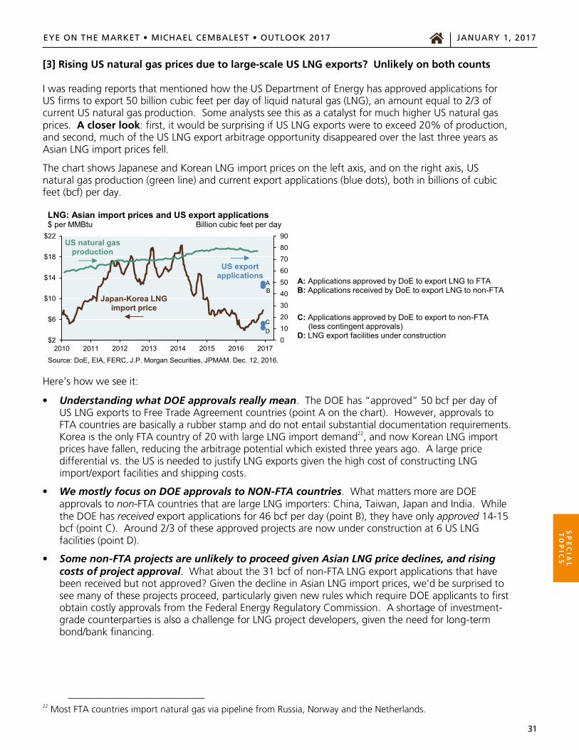
The chart shows Japanese and Korean LNG import prices on the left axis, and on the right axis, US natural gas production (green line) and current export applications (blue dots), both in billions of cubic feet (bcf) per day.

Here’s how we see it:

• Understanding what DOE approvals really mean. The DOE has “approved” 50 bcf per day of US LNG exports to Free Trade Agreement countries (point A on the chart). However, approvals to FTA countries are basically a rubber stamp and do not entail substantial documentation requirements. Korea is the only FTA country of 20 with large LNG import demand22, and now Korean LNG import prices have fallen, reducing the arbitrage potential which existed three years ago. A large price differential vs. the US is needed to justify LNG exports given the high cost of constructing LNG import/export facilities and shipping costs.

• We mostly focus on DOE approvals to NON-FTA countries. What matters more are DOE approvals to non-FTA countries that are large LNG importers: China, Taiwan, Japan and India. While the DOE has received export applications for 46 bcf per day (point B), they have only approved 14-15 bcf (point C). Around 2/3 of these approved projects are now under construction at 6 US LNG facilities (point D).

• Some non-FTA projects are unlikely to proceed given Asian LNG price declines, and rising costs of project approval. What about the 31 bcf of non-FTA LNG export applications that have been received but not approved? Given the decline in Asian LNG import prices, we’d be surprised to see many of these projects proceed, particularly given new rules which require DOE applicants to first obtain costly approvals from the Federal Energy Regulatory Commission. A shortage of investment-grade counterparties is also a challenge for LNG project developers, given the need for long-term bond/bank financing.

22 Most FTA countries import natural gas via pipeline from Russia, Norway and the Netherlands.

A: Applications approved by DoE to export LNG to FTAB: Applications received by DoE to export LNG to non-FTA

C: Applications approved by DoE to export to non-FTA (less contingent approvals)

D: LNG export facilities under construction0102030405060708090

$2

$6

$10

$14

$18

$22

2010 2011 2012 2013 2014 2015 2016 2017

Source: DoE, EIA, FERC, J.P. Morgan Securities, JPMAM. Dec. 12, 2016.

LNG: Asian import prices and US export applications$ per MMBtu Billion cubic feet per day

Japan-Korea LNG import price

US export applications

US natural gasproduction

B

CD

A

SP

EC

IAL

T

OP

ICS


32

SP

EC

IAL

T

OP

ICS


32

• How does the DOE make decisions on LNG export projects? The DOE takes a lot of things into account when considering non-FTA approvals, including the adequacy of the domestic natural gas supply, US energy security, impacts on the US economy (particularly the cost of electricity23 and gas-related input costs for manufacturers), international considerations and environmental impacts. As part of this process, the DOE issued a study in October 2015 that considered the macroeconomic impact of US LNG exports reaching 20 bcf per day, which may represent an upper bound in their thinking on the subject. Their primary conclusion: any increase in US LNG exports would mostly result from increases in US domestic production, and not result in much higher US prices or constrained demand.

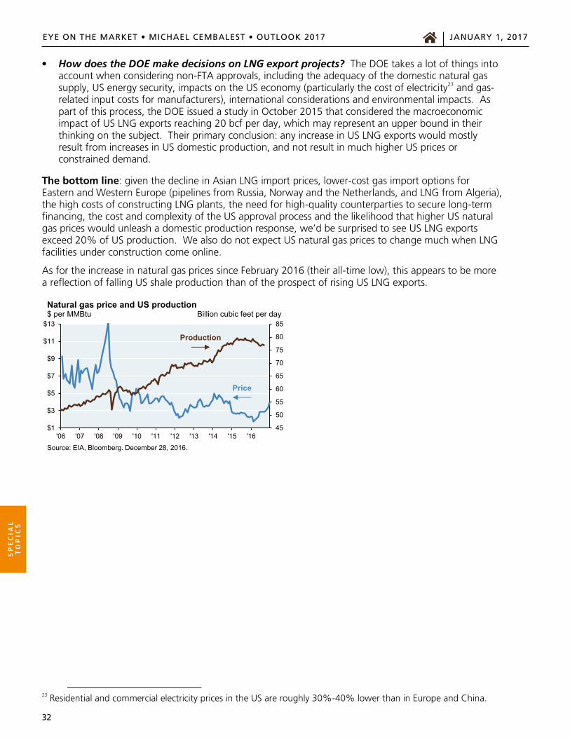
The bottom line: given the decline in Asian LNG import prices, lower-cost gas import options for Eastern and Western Europe (pipelines from Russia, Norway and the Netherlands, and LNG from Algeria), the high costs of constructing LNG plants, the need for high-quality counterparties to secure long-term financing, the cost and complexity of the US approval process and the likelihood that higher US natural gas prices would unleash a domestic production response, we’d be surprised to see US LNG exports exceed 20% of US production. We also do not expect US natural gas prices to change much when LNG facilities under construction come online.

As for the increase in natural gas prices since February 2016 (their all-time low), this appears to be more a reflection of falling US shale production than of the prospect of rising US LNG exports.

23 Residential and commercial electricity prices in the US are roughly 30%-40% lower than in Europe and China.

45

50

55

60

65

70

75

80

85

$1

$3

$5

$7

$9

$11

$13

'06 '07 '08 '09 '10 '11 '12 '13 '14 '15 '16

Source: EIA, Bloomberg. December 28, 2016.

Natural gas price and US production$ per MMBtu Billion cubic feet per day

Production

Price


33

SP

EC

IAL

T

OP

ICS


33

0%

20%

40%

60%

80%

100%

'02 '03 '04 '05 '06 '07 '08 '09 '10

ST capital loss LT capital gain LT capital loss ST capital gain

Source: Parametric Portfolio, JPMAM. Q4 2015. Shown for illustrative purposes only. Past performance is not indicative of future results.

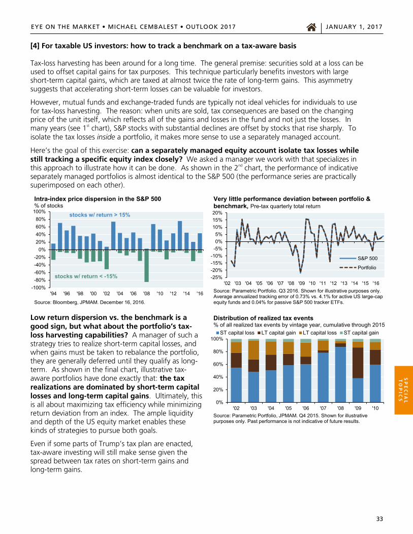
Distribution of realized tax events% of all realized tax events by vintage year, cumulative through 2015

[4] For taxable US investors: how to track a benchmark on a tax-aware basis Tax-loss harvesting has been around for a long time. The general premise: securities sold at a loss can be used to offset capital gains for tax purposes. This technique particularly benefits investors with large short-term capital gains, which are taxed at almost twice the rate of long-term gains. This asymmetry suggests that accelerating short-term losses can be valuable for investors.

However, mutual funds and exchange-traded funds are typically not ideal vehicles for individuals to use for tax-loss harvesting. The reason: when units are sold, tax consequences are based on the changing price of the unit itself, which reflects all of the gains and losses in the fund and not just the losses. In many years (see 1st chart), S&P stocks with substantial declines are offset by stocks that rise sharply. To isolate the tax losses inside a portfolio, it makes more sense to use a separately managed account.

Here’s the goal of this exercise: can a separately managed equity account isolate tax losses while still tracking a specific equity index closely? We asked a manager we work with that specializes in this approach to illustrate how it can be done. As shown in the 2nd chart, the performance of indicative separately managed portfolios is almost identical to the S&P 500 (the performance series are practically superimposed on each other).

Low return dispersion vs. the benchmark is a good sign, but what about the portfolio’s tax- loss harvesting capabilities? A manager of such a strategy tries to realize short-term capital losses, and when gains must be taken to rebalance the portfolio, they are generally deferred until they qualify as long-term. As shown in the final chart, illustrative tax-aware portfolios have done exactly that: the tax realizations are dominated by short-term capital losses and long-term capital gains. Ultimately, this is all about maximizing tax efficiency while minimizing return deviation from an index. The ample liquidity and depth of the US equity market enables these kinds of strategies to pursue both goals.

Even if some parts of Trump’s tax plan are enacted, tax-aware investing will still make sense given the spread between tax rates on short-term gains and long-term gains.

-100%-80%-60%-40%-20%

0%20%40%60%80%

100%

'94 '96 '98 '00 '02 '04 '06 '08 '10 '12 '14 '16

Source: Bloomberg, JPMAM. December 16, 2016.

Intra-index price dispersion in the S&P 500% of stocks

stocks w/ return > 15%

stocks w/ return < -15% -25%-20%-15%-10%-5%0%5%

10%15%20%

'02 '03 '04 '05 '06 '07 '08 '09 '10 '11 '12 '13 '14 '15 '16

S&P 500

Portfolio

Source: Parametric Portfolio. Q3 2016. Shown for illustrative purposes only. Average annualized tracking error of 0.73% vs. 4.1% for active US large-cap equity funds and 0.04% for passive S&P 500 tracker ETFs.

Very little performance deviation between portfolio & benchmark, Pre-tax quarterly total return


34

SP

EC

IAL

T

OP

ICS


34

[5] Infrastructure investing and the role for public-private partnerships The GOP and Democrats seem to agree that infrastructure investment is a high priority. However, there’s disagreement about how to do it. Clinton’s plan relied on direct government spending on infrastructure, financed through taxes on accumulated and untaxed offshore corporate profits. Trump’s plan appears to rely more on private sector investment by offering tax breaks to private enterprises to construct and operate new revenue generating projects in concert with public agencies (i.e. public-private partnerships, or PPPs). Some commentators have criticized Trump’s plan (Krugman called it “basically fraudulent”24 and Sanders described it as “corporate welfare”25). However, there are ways that PPPs can drive infrastructure investing, particularly if the use of proceeds is to finance new greenfield projects. It all depends on the details.

Let’s start with the recognition that the current system does not produce the necessary amount of US infrastructure spending26. Since Federal debt ratios are close to the highest levels since WWII and since most municipalities are constrained on spending (due to unfunded pension and retiree healthcare costs), some analysts believe that PPPs can play an important role. In fact, Obama’s Treasury department issued a report in 2015 on the subject which strongly endorses PPPs as a means of building infrastructure for the future27. Here are some of its conclusions:

“The need to reverse years of underinvestment in infrastructure, despite tighter budgets at every level of government, calls for us to rethink how we pay for and manage infrastructure investment”

“When the private sector takes on risks that it can manage more cost-effectively, a PPP may be able to save money for taxpayers and deliver higher quality or more reliable service over a shorter timeframe compared to traditional procurement”

“When sponsors contract with private partners that support strong labor standards, PPPs can also provide local economic opportunity and create good, middle-class jobs that benefit current and aspiring workers alike”

“While PPPs cannot eliminate the need for government spending on infrastructure, we can help meet our nation’s infrastructure needs by expanding the sources of investment and using those dollars, whether public or private, as effectively as possible to advance the public’s interest”

“Other advanced economies, including Australia, Canada, and the United Kingdom, rely more heavily than the United States on PPPs to secure equity financing for infrastructure”

“Although the role of PPPs in the US market is limited, the US Department of the Treasury’s research and engagement with stakeholders indicate that significant private capital could be mobilized for infrastructure investment”

“However, in order to attract this capital, US public infrastructure assets will have to support higher rates of return than are currently generated through 100 percent low-cost debt financing in the municipal bond market”

24 “Build He Won’t”, Paul Krugman, New York Times, November 21, 2016. 25 “Let’s Rebuild our Infrastructure, Not Provide Tax Breaks to Big Corporations and Wall Street”, Bernie Sanders, Medium.com, Nov. 21, 2016. 26 In 2013, the American Society of Civil Engineers graded the United States infrastructure in a 74-page report. The grades: B- for solid waste, C+ for bridges & railways, C for ports, D+ for energy, D for aviation systems, dams, drinking and waste water, schools, transit, and roads, and D- for inland waterways and levees. 27 “Expanding the market for infrastructure public-private partnerships: alternative risk and profit sharing approaches to align sponsor and investor interests”, US Department of the Treasury, April 2015.

Stro

ng

PPP

en

do

rsem

ent

fro

m t

he

Ob

ama

adm

inis

trat

ion


35

SP

EC

IAL

T

OP

ICS


35

I asked our infrastructure group at J.P. Morgan Asset Management to weigh in on the subject. Here’s what they had to say about PPPs:

PPPs require some combination of federal grants, taxes and user fees to incent private capital to participate. This framework has to exist before PPPs can be launched, and must often be preceded by political outreach to gain support from taxpayers and other constituents. While user fees often seem like a nuisance or private sector profiteering, they are essentially a replacement for public sector spending and related taxes paid by citizens

While the privatization of existing assets may not appear to generate much in the way of investment or hiring on the asset privatized, the use of proceeds can accelerate greenfield (new) projects that have higher multiplier effects

In principle, a PPP that allocates responsibilities optimally would have governments deal with legislation, jurisdictional considerations, procurement, permitting, siting, appeals, etc28. Then, private sector operators would focus on project delivery and management

There are examples of successful PPPs, some of which have taken place outside the US, as noted in the Treasury report:

o Local privatization of 11 Canadian airports, with the Ministry of Infrastructure quid pro quo that it be able to use proceeds for new greenfield projects

o Australian infrastructure program, in which existing infrastructure assets are sold to finance the construction of new projects at the national and local level (similar in concept to Canada)

o In the UK, the £4.2 billion Thames Tideway wastewater project was financed through a PPP which took advantage of low interest rates on project financing. The UK government took the timing and construction cost overrun risk (immunizing private sector capital from a Boston-esque “Big Dig” outcome), which then lowered the return requirement for private capital. The UK intends to use the same approach for future electricity transmission and aquifer projects

o In Texas, with guidance and direction from government entities, private capital (a combination of utilities, cooperatives and private investors) financed $7 bn of wind farm transmission lines from 2007 to 2013, supporting Texas’ 18.5 GW of installed wind capacity, the highest in the US

o In Los Angeles, major public transit projects are being financed in part by an increase in the sales tax until 2062, based on a bill approved this fall. Projects include extending light rail to LAX, extending the subway to Westwood, earthquake retrofits and highway improvements. Projected tax proceeds of $120 bn will be used as the government’s contribution to projects that also entail private sector capital and private sector project management and construction (thereby limiting permanent employment increases for California’s public sector)

o Denver’s airport train system received a $1 bn Federal grant as part of a larger PPP in which private sector bidders identified design efficiencies that resulted in significant cost savings (one example: double tracking wasn’t necessary for the entire route given train frequencies); the grant would not have been available if it were a public-only project

28 A good example of the constructive role that government can play: the Path-15 electricity transmission project in California. An impasse between the California Energy Commission and the California Public Utilities Commission had prevented improvement of transmission bottlenecks that led to blackouts in 1996 and 2001. The Western Area Power Administration (a Federal entity) was able to use the threat of jurisdiction and eminent domain to get both parties to the table to complete the project.


36

SP

EC

IAL

T

OP

ICS


36

[6] The biggest problem with “clean coal”: scope “Clean coal” is a euphemism for coal powered electricity in which carbon capture and storage of CO2 takes place (CCS). By the end of 2016, CCS facilities in operation will be able to capture and store just 0.1% of the world’s CO2 emissions. Let’s put aside issues of large cost overruns on recent projects29, the Department of Energy withdrawing support from several large projects (FutureGen in Illinois), project cancellations in Europe, legal uncertainties about liability associated with CO2 leaks, evidence of leakage and earthquake risk from CCS operations in the Middle East and the North Sea, and the ~30% energy drag on coal facilities required to perform CCS in the first place.

Let’s assume that all of these problems can be solved via technological innovation and legislation (an aggressive assumption, for sure). The bigger problem with CCS is the scope required to make a difference. To see why, let’s assume the world aims to sequester just 15% of global CO2 emissions.

In 2015, global CO2 emissions were 33.5 billion tonnes To sequester 15%, that would mean capturing, transporting and burying 5.0 billion tonnes of CO2 That amount of CO2 by weight is equivalent to 6.3 billion cubic meters of CO2 by volume (assuming

0.8 tonnes per cubic meter of CO2 when compressed) How much volume is that? Global crude oil extraction in 2015 was 4.4 billion tonnes by weight,

which is equivalent to around 5.1 billion cubic meters of oil by volume

Compare the two bolded numbers above, and you can see the problem. Even capturing a small portion of global CO2 emissions would require a CO2 compression/transportation/storage industry whose throughput is even greater than the one used for the world’s oil transportation and refining, which has taken 100 years to build (see map); and that’s without the benefit that oil provides as an energy input to vehicle transportation and industry. There may be applications where CCS makes sense (enhanced oil recovery, and meeting small amounts of commercial CO2 demand). But as a big picture solution to CO2 emissions, CCS infrastructure needs and costs are very daunting. Global oil pipeline and refining networks

Source: Rextag. November 2016.

29 According to the New York Times, the Kemper clean coal plant in Mississippi is more than two years behind schedule, more than $4 billion over its initial budget of $2.4 billion, and still not operational.


37

SP

EC

IAL

T

OP

ICS


37

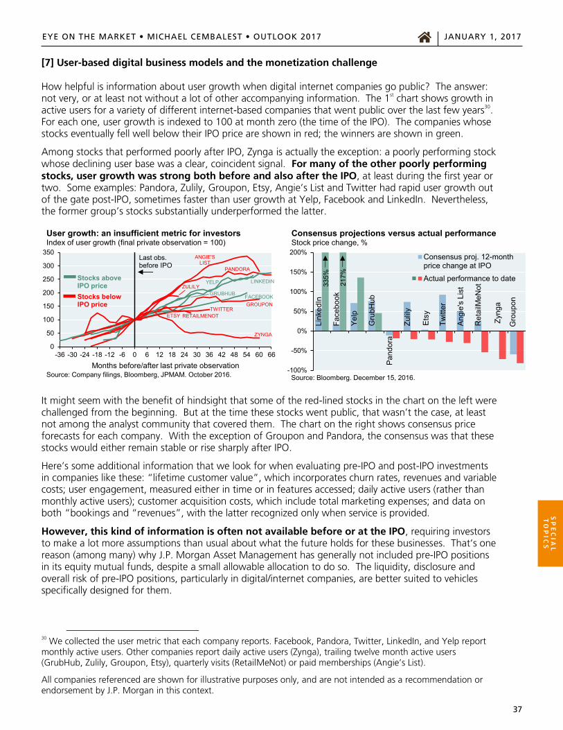
[7] User-based digital business models and the monetization challenge How helpful is information about user growth when digital internet companies go public? The answer: not very, or at least not without a lot of other accompanying information. The 1st chart shows growth in active users for a variety of different internet-based companies that went public over the last few years30. For each one, user growth is indexed to 100 at month zero (the time of the IPO). The companies whose stocks eventually fell well below their IPO price are shown in red; the winners are shown in green.

Among stocks that performed poorly after IPO, Zynga is actually the exception: a poorly performing stock whose declining user base was a clear, coincident signal. For many of the other poorly performing stocks, user growth was strong both before and also after the IPO, at least during the first year or two. Some examples: Pandora, Zulily, Groupon, Etsy, Angie’s List and Twitter had rapid user growth out of the gate post-IPO, sometimes faster than user growth at Yelp, Facebook and LinkedIn. Nevertheless, the former group’s stocks substantially underperformed the latter.

It might seem with the benefit of hindsight that some of the red-lined stocks in the chart on the left were challenged from the beginning. But at the time these stocks went public, that wasn’t the case, at least not among the analyst community that covered them. The chart on the right shows consensus price forecasts for each company. With the exception of Groupon and Pandora, the consensus was that these stocks would either remain stable or rise sharply after IPO.

Here’s some additional information that we look for when evaluating pre-IPO and post-IPO investments in companies like these: “lifetime customer value”, which incorporates churn rates, revenues and variable costs; user engagement, measured either in time or in features accessed; daily active users (rather than monthly active users); customer acquisition costs, which include total marketing expenses; and data on both “bookings and “revenues”, with the latter recognized only when service is provided.

However, this kind of information is often not available before or at the IPO, requiring investors to make a lot more assumptions than usual about what the future holds for these businesses. That‘s one reason (among many) why J.P. Morgan Asset Management has generally not included pre-IPO positions in its equity mutual funds, despite a small allowable allocation to do so. The liquidity, disclosure and overall risk of pre-IPO positions, particularly in digital/internet companies, are better suited to vehicles specifically designed for them.

30 We collected the user metric that each company reports. Facebook, Pandora, Twitter, LinkedIn, and Yelp report monthly active users. Other companies report daily active users (Zynga), trailing twelve month active users (GrubHub, Zulily, Groupon, Etsy), quarterly visits (RetailMeNot) or paid memberships (Angie’s List).

All companies referenced are shown for illustrative purposes only, and are not intended as a recommendation or endorsement by J.P. Morgan in this context.

0

50

100

150

200

250

300

350

-36 -30 -24 -18 -12 -6 0 6 12 18 24 30 36 42 48 54 60 66Months before/after last private observation

Source: Company filings, Bloomberg, JPMAM. October 2016.

User growth: an insufficient metric for investors Index of user growth (final private observation = 100)

Stocks above IPO price

Last obs. before IPO

LINKEDINYELP

GROUPON

PANDORA

FACEBOOK

TWITTERRETAILMENOT

ZYNGA

GRUBHUBZULILY

ETSY

ANGIE'S LIST

Stocks below IPO price

Link

edIn

Face

book

Yelp

Gru

bHub

Pand

ora

Zulil

y

Etsy

Twitt

er

Angi

e's

List

Ret

ailM

eNot

Zyng

a

Gro

upon

-100%

-50%

0%

50%

100%

150%

200% Consensus proj. 12-monthprice change at IPO

Actual performance to date

Source: Bloomberg. December 15, 2016.

Consensus projections versus actual performanceStock price change, %

335%

217%


38

SP

EC

IAL

T

OP

ICS


38

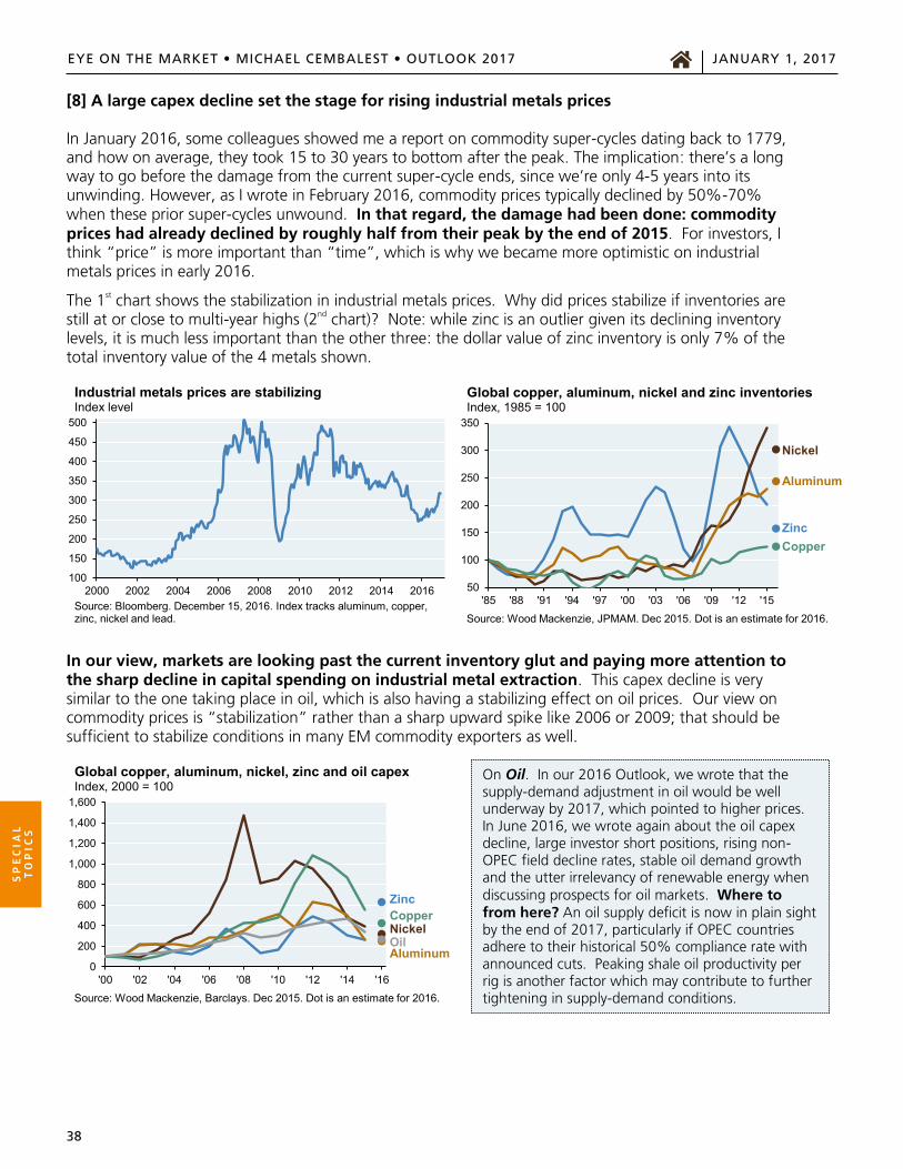
[8] A large capex decline set the stage for rising industrial metals prices In January 2016, some colleagues showed me a report on commodity super-cycles dating back to 1779, and how on average, they took 15 to 30 years to bottom after the peak. The implication: there’s a long way to go before the damage from the current super-cycle ends, since we’re only 4-5 years into its unwinding. However, as I wrote in February 2016, commodity prices typically declined by 50%-70% when these prior super-cycles unwound. In that regard, the damage had been done: commodity prices had already declined by roughly half from their peak by the end of 2015. For investors, I think “price” is more important than “time”, which is why we became more optimistic on industrial metals prices in early 2016.

The 1st chart shows the stabilization in industrial metals prices. Why did prices stabilize if inventories are still at or close to multi-year highs (2nd chart)? Note: while zinc is an outlier given its declining inventory levels, it is much less important than the other three: the dollar value of zinc inventory is only 7% of the total inventory value of the 4 metals shown.

In our view, markets are looking past the current inventory glut and paying more attention to the sharp decline in capital spending on industrial metal extraction. This capex decline is very similar to the one taking place in oil, which is also having a stabilizing effect on oil prices. Our view on commodity prices is “stabilization” rather than a sharp upward spike like 2006 or 2009; that should be sufficient to stabilize conditions in many EM commodity exporters as well.

100

150

200

250

300

350

400

450

500

2000 2002 2004 2006 2008 2010 2012 2014 2016Source: Bloomberg. December 15, 2016. Index tracks aluminum, copper, zinc, nickel and lead.

Industrial metals prices are stabilizingIndex level

50

100

150

200

250

300

350

'85 '88 '91 '94 '97 '00 '03 '06 '09 '12 '15

Source: Wood Mackenzie, JPMAM. Dec 2015. Dot is an estimate for 2016.

Global copper, aluminum, nickel and zinc inventoriesIndex, 1985 = 100

ZincCopper

Nickel

Aluminum

0

200

400

600

800

1,000

1,200

1,400

1,600

'00 '02 '04 '06 '08 '10 '12 '14 '16

Source: Wood Mackenzie, Barclays. Dec 2015. Dot is an estimate for 2016.

Global copper, aluminum, nickel, zinc and oil capexIndex, 2000 = 100

ZincCopperNickel

AluminumOil

On Oil. In our 2016 Outlook, we wrote that the supply-demand adjustment in oil would be well underway by 2017, which pointed to higher prices. In June 2016, we wrote again about the oil capex decline, large investor short positions, rising non-OPEC field decline rates, stable oil demand growth and the utter irrelevancy of renewable energy when discussing prospects for oil markets. Where to from here? An oil supply deficit is now in plain sight by the end of 2017, particularly if OPEC countries adhere to their historical 50% compliance rate with announced cuts. Peaking shale oil productivity per rig is another factor which may contribute to further tightening in supply-demand conditions.


39

SP

EC

IAL

T

OP

ICS


39

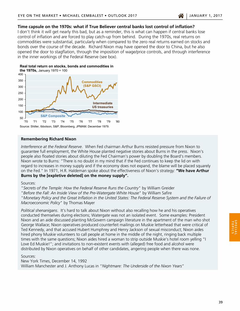
Time capsule on the 1970s: what if True Believer central banks lost control of inflation? I don’t think it will get nearly this bad, but as a reminder, this is what can happen if central banks lose control of inflation and are forced to play catch-up from behind. During the 1970s, real returns on commodities were substantial, particularly when compared to the zero real returns earned on stocks and bonds over the course of the decade. Richard Nixon may have opened the door to China, but he also opened the door to stagflation, through the imposition of wage/price controls, and through interference in the inner workings of the Federal Reserve (see box).

50

100

150

200

250

300

350

400

'70 '71 '72 '73 '74 '75 '76 '77 '78 '79 '80

Source: Shiller, Ibbotson, S&P, Bloomberg, JPMAM. December 1979.

Real total return on stocks, bonds and commodities in the 1970s, January 1970 = 100

S&P Composite

Intermediate US treasuries

Commodities (S&P GSCI)

Remembering Richard Nixon

Interference at the Federal Reserve. When Fed chairman Arthur Burns resisted pressure from Nixon to guarantee full employment, the White House planted negative stories about Burns in the press. Nixon’s people also floated stories about diluting the Fed Chairman’s power by doubling the Board’s members. Nixon wrote to Burns: “There is no doubt in my mind that if the Fed continues to keep the lid on with regard to increases in money supply and if the economy does not expand, the blame will be placed squarely on the Fed.” In 1971, H.R. Haldeman spoke about the effectiveness of Nixon’s strategy: “We have Arthur Burns by the [expletive deleted] on the money supply”.

Sources: "Secrets of the Temple: How the Federal Reserve Runs the Country" by William Greider "Before the Fall: An Inside View of the Pre-Watergate White House" by William Safire "Monetary Policy and the Great Inflation in the United States: The Federal Reserve System and the Failure of Macroeconomic Policy" by Thomas Mayer

Political shenanigans. It’s hard to talk about Nixon without also recalling how he and his operatives conducted themselves during elections; Watergate was not an isolated event. Some examples: President Nixon and an aide discussed planting McGovern campaign literature in the apartment of the man who shot George Wallace; Nixon operatives produced counterfeit mailings on Muskie letterhead that were critical of Ted Kennedy, and that accused Hubert Humphrey and Henry Jackson of sexual misconduct; Nixon aides hired phony Muskie volunteers to call people at home in the middle of the night, ringing back multiple times with the same questions; Nixon aides hired a woman to strip outside Muskie’s hotel room yelling “I Love Ed Muskie!”; and invitations to non-existent events with (alleged) free food and alcohol were distributed by Nixon operatives on behalf of other candidates, angering people when there was none.

Sources: New York Times, December 14, 1992 William Manchester and J. Anthony Lucas in “Nightmare: The Underside of the Nixon Years”

EYE ON THE MARKET • MICHAEL CEMBALEST • OUTLOOK 2017 JANUARY 1, 2017EYE ON THE MARKET MICHAEL CEMBALEST OUTLOOK 2017 JANUARY 1, 2017

41

IMPORTANT INFORMATION Purpose of This Material: This material is for information purposes only.

The views, opinions, estimates and strategies expressed herein constitutes Michael Cembalest’s judgment based on current market conditions and are subject to change without notice, and may differ from those expressed by other areas of J.P. Morgan. This information in no way constitutes J.P. Morgan Research and should not be treated as such. Any projected results and risks are based solely on hypothetical examples cited, and actual results and risks will vary depending on specific circumstances. We believe certain information contained in this material to be reliable but do not warrant its accuracy or completeness. We do not make any representation or warranty with regard to any computations, graphs, tables, diagrams or commentary in this material which is provided for illustration/reference purposes only. Investors may get back less than they invested, and past performance is not a reliable indicator of future results. It is not possible to invest directly in an index. Forward looking statements should not be considered as guarantees or predictions of future events.

Confidentiality: This material is confidential and intended for your personal use. It should not be circulated to or used by any other person, or duplicated for non-personal use, without our permission.

Regulatory Status: In the United States, Bank products and services, including certain discretionary investment management products and services, are offered by JPMorgan Chase Bank, N.A. and its affiliates. Securities products and services are offered in the U.S. by J.P. Morgan Securities LLC, an affiliate of JPMCB, and outside of the U.S. by other global affiliates. J.P. Morgan Securities LLC, member FINRA and SIPC.

In the United Kingdom, this material is issued by J.P. Morgan International Bank Limited (JPMIB) with the registered office located at 25 Bank Street, Canary Wharf, London E14 5JP, registered in England No. 03838766. JPMIB is authorised by the Prudential Regulation Authority and regulated by the Financial Conduct Authority and the Prudential Regulation Authority. In addition, this material may be distributed by: JPMorgan Chase Bank, N.A. (“JPMCB”), Paris branch, which is regulated by the French banking authorities Autorité de Contrôle Prudentiel et de Résolution and Autorité des Marchés Financiers; J.P. Morgan (Suisse) SA, regulated by the Swiss Financial Market Supervisory Authority; JPMCB Dubai branch, regulated by the Dubai Financial Services Authority; JPMCB Bahrain branch, licensed as a conventional wholesale bank by the Central Bank of Bahrain (for professional clients only).

In Hong Kong, this material is distributed by JPMCB, Hong Kong branch. JPMCB, Hong Kong branch is regulated by the Hong Kong Monetary Authority and the Securities and Futures Commission of Hong Kong. In Hong Kong, we will cease to use your personal data for our marketing purposes without charge if you so request. In Singapore, this material is distributed by JPMCB, Singapore branch. JPMCB, Singapore branch is regulated by the Monetary Authority of Singapore. Dealing and advisory services and discretionary investment management services are provided to you by JPMCB, Hong Kong/Singapore branch (as notified to you). Banking and custody services are provided to you by JPMIB and/ or JPMCB Singapore Branch. The contents of this document have not been reviewed by any regulatory authority in Hong Kong, Singapore or any other jurisdictions. You are advised to exercise caution in relation to this document. If you are in any doubt about any of the contents of this document, you should obtain independent professional advice.

With respect to countries in Latin America, the distribution of this material may be restricted in certain jurisdictions. Receipt of this material does not constitute an offer or solicitation to any person in any jurisdiction in which such offer or solicitation is not authorized or to any person to whom it would be unlawful to make such offer or solicitation.

Risks, Considerations and Additional information: There may be different or additional factors which are not reflected in this material, but which may impact on a client’s portfolio or investment decision. The information contained in this material is intended as general market commentary and should not be relied upon in isolation for the purpose of making an investment decision. Nothing in this document shall be construed as giving rise to any duty of care owed to, or advisory relationship with, you or any third party. Nothing in this document is intended to constitute a representation that any investment strategy or product is suitable for you. You should consider carefully whether any products and strategies discussed are suitable for your needs, and to obtain additional information prior to making an investment decision. Nothing in this document shall be regarded as an offer, solicitation, recommendation or advice (whether financial, accounting, legal, tax or other) given by J.P. Morgan and/or its officers or employees, irrespective of whether or not such communication was given at your request.

J.P. Morgan and its affiliates and employees do not provide tax, legal or accounting advice. You should consult your own tax, legal and accounting advisors before engaging in any financial transactions. Contact your J.P. Morgan representative for additional information concerning your personal investment goals. You should be aware of the general and specific risks relevant to the matters discussed in the material. You will independently, without any reliance on J.P. Morgan, make your own judgment and decision with respect to any investment referenced in this material.

J.P. Morgan may hold a position for itself or our other clients which may not be consistent with the information, opinions, estimates, investment strategies or views expressed in this document.

JPMorgan Chase & Co. or its affiliates may hold a position or act as market maker in the financial instruments of any issuer discussed herein or act as an underwriter, placement agent, advisor or lender to such issuer.

References in this report to “J.P. Morgan” are to JPMorgan Chase & Co., its subsidiaries and affiliates worldwide. “J.P. Morgan Private Bank” is the marketing name for the private banking business conducted by J.P. Morgan.

If you have any questions or no longer wish to receive these communications, please contact your usual J.P. Morgan representative.

© 2017 JPMorgan Chase & Co. All rights reserved. 1016-0947-01

2017 Eye on the Market Outlook Special Topics - J.P. Morgan · 2017 Eye on the Market Outlook...

Documents

Transcript of 2017 Eye on the Market Outlook Special Topics - J.P. Morgan · 2017 Eye on the Market Outlook...