
2016 EU Wide Stress Test - Home - European Banking …EU-wide...2016 EU‐WIDE STRESS TEST –...
119
2016 EU‐WIDE STRESS TEST – METHODOLOGICAL NOTE 2016 EU‐Wide Stress Test Methodological Note 24 February 2016
Transcript of 2016 EU Wide Stress Test - Home - European Banking …EU-wide...2016 EU‐WIDE STRESS TEST –...

2016 EU‐WIDE STRESS TEST – METHODOLOGICAL NOTE
2016 EU‐Wide Stress Test
Methodological Note
24 February 2016
2016 EU‐WIDE STRESS TEST – METHODOLOGICAL NOTE
2
Contents
List of figures 5
Abbreviations 7
1. Introduction 9
1.1 Background 9
1.2 Objectives of this note 9
1.3 Key aspects 9
1.3.1 Sample of banks 9 1.3.2 Scope of consolidation 10 1.3.3 Macroeconomic scenarios and risk type specific shocks 10 1.3.4 Time horizon and reference date 11 1.3.5 Definition of capital 11 1.3.6 Hurdle rates 12 1.3.7 Accounting and tax regime 12 1.3.8 Static balance sheet assumption 12 1.3.9 Approach 13 1.3.10 Risk coverage 13 1.3.11 Process 14 1.3.12 Overview of the methodology by risk type 15
2. Credit risk 19
2.1 Overview 19
2.2 Scope 20
2.3 High‐level assumptions and definitions 20
2.3.1 Definitions 20 2.3.2 Static balance sheet assumption 24 2.3.3 Asset classes 25 2.3.4 Reporting requirements 27
2.4 Impact on P&L 27
2.4.1 Starting point‐in‐time risk parameters (a hierarchy of approaches) 27 2.4.2 Projected point‐in‐time parameters (a hierarchy of approaches) 28 2.4.3 Calculation of defaulted assets and impairments 33
a. Impairment losses on new defaulted assets 33 b. Impairment losses on old defaulted assets 34 c. Impairment losses on sovereign exposures 35
2.4.4 FX lending 35
2.5 Impact on REA and IRB regulatory EL 36
2.6 REA for CCR 37
2.7 Securitisation exposures 38
3. Market risk, CCR losses and CVA 41
2016 EU‐WIDE STRESS TEST – METHODOLOGICAL NOTE
3
3.1 Overview 41
3.2 Scope 42
3.3 High‐level assumptions and definitions 43
3.3.1 Definitions 43 3.3.2 Static balance sheet assumption 46 3.3.3 Application of the SA and the CA 46 3.3.4 Reference date and time horizon 46
3.4 Treatment of hedging 47
3.5 Market risk factors 51
3.6 Impact on P&L and OCI – AFS and FVO positions 55
3.6.1 Non‐sovereign 56 3.6.2 Sovereign 56
3.7 Impact on P&L – HFT positions 57
3.7.1 Starting value of the NTI 57 3.7.2 CA 58 3.7.3 SA 61
3.8 CCR losses and CVA losses 62
3.8.1 CVA impact on P&L and exclusion of the DVA impact 62 3.8.2 Counterparty defaults 63
3.9 Impact on REA 65
4. NII 68
4.1 Overview 68
4.2 Scope 69
4.3 High‐level assumptions and definitions 70
4.3.1 Definitions 70 4.3.2 Static balance sheet assumption 71 4.3.3 Treatment of maturing assets and liabilities 72 4.3.1 Curve and currency shocks 76 4.3.2 Reporting requirements 76
4.4 Impact on P&L 77
4.4.1 High‐level constraints on NII 77 4.4.2 Interest on defaulted loans 78 4.4.3 Projection of the components of the EIR 81
a. Constraints on the margin component for liability positions 84 b. Constraints on the margin component for asset positions 86
5. Conduct risk and other operational risks 88
5.1 Overview 88
5.2 Scope 89
5.3 High‐level assumptions and definitions 89
5.3.1 Definitions 89 5.3.2 Reporting requirements 90
2016 EU‐WIDE STRESS TEST – METHODOLOGICAL NOTE
4
5.4 Impact on P&L 92
5.4.1 Conduct risk treatment 92 a. Qualitative approach to estimating future conduct risk losses 93 b. Quantitative approach to estimating future conduct risk losses 95 c. Floor for conduct risk loss projections 95
5.4.2 Treatment of other operational risks 96 5.4.3 Fall‐back solution 96
5.5 Impact on capital requirements 97
5.5.1 AMA 97 5.5.2 Basic approach and standard approach 97
6. Non‐interest income, expenses and capital 98
6.1 Overview 98
6.2 Scope 99
6.3 High‐level assumptions and definitions 100
6.3.1 Definitions 100 6.3.2 Approach 100 6.3.3 Reporting requirements 100
6.4 Impact on P&L and capital 101
6.4.1 Dividend income and net fee and commission income 101 6.4.2 Administrative expenses, profit or loss from discontinued operations, and other operating expenses 101 6.4.3 Dividends paid 103 6.4.4 Other P&L and capital items 103
Annex I: Sample of banks 106
Annex II: Template overview 108
Annex III: Summary of qualitative information to be provided by banks 110
Annex IV: Summary of key constraints and other quantitative requirements 114
2016 EU‐WIDE STRESS TEST – METHODOLOGICAL NOTE
5
List of figures
Table 1: Overview of the methodology by risk type ........................................................................ 15
Box 1: Summary of the constraints on banks’ projections of credit risk ......................................... 19
Table 2: Overview of IRB asset classes ............................................................................................. 25
Table 3: Overview of STA asset classes ............................................................................................ 26
Box 2: Example of the outcome of applying point‐in‐time migration matrices to different portfolio structures ......................................................................................................................................... 29
Box 3: Impairment losses on new defaulted assets ......................................................................... 33
Box 4: Impairment losses on old defaulted assets ........................................................................... 34
Table 4: FX lending threshold (per country of counterparty) – IRB asset classes ............................ 36
Table 5: FX lending threshold (per country of counterparty) – STA asset classes ........................... 36
Box 5: REA estimation for defaulted assets ..................................................................................... 37
Box 6: Summary of the constraints on banks’ projections of market risk ....................................... 42
Box 7: Definition of the scaling factor that accounts for economic hedges .................................... 49
Box 8: Example of the application of the scaling factor that accounts for economic hedges ......... 50
Box 9: Treatment of additional risk factors ...................................................................................... 53
Box 10: Definition of the starting NTI value ..................................................................................... 57
Box 11: Formalised description of the comprehensive market risk stress approach ...................... 58
Box 12: Formalised description of a simplified market risk stress approach ................................... 61
Box 13: Algorithm for identifying and defaulting CCR exposures .................................................... 65
Table 6: VaR assumptions for the calculation of the REA ................................................................ 66
Box 14: Summary of the constraints on banks’ projections of NII ................................................... 68
Box 15: Calculation of volumes – Illustration ................................................................................... 74
Box 16: Application of the materiality constraint on the currency/country breakdown requested 77
Box 17: Treatment of discount unwinding ....................................................................................... 78
Table 7: Mapping of the IRB credit risk asset class to the NII asset type ......................................... 79
Table 8: Mapping of the STA credit risk asset class to the NII asset type ........................................ 80
Box 18: Calculation of the NII – Illustration ..................................................................................... 83
Box 19: Floor for the evolution of the margin paid on new liabilities (pass‐through constraint) ... 84
Box 20: Cap on the evolution of the margin earned on new assets (pass‐through constraint) ...... 87
2016 EU‐WIDE STRESS TEST – METHODOLOGICAL NOTE
6
Box 21: Summary of the constraints on banks’ projections of conduct risk and other operational risks .................................................................................................................................................. 88
Table 9: Projection of conduct risk losses under the qualitative approach and in the adverse scenario – Illustration ....................................................................................................................... 94
Box 22: Floor for conduct risk losses ................................................................................................ 95
Box 23: Floor for the projection of other operational risk losses .................................................... 96
Box 24: Fall‐back solution for other operational risk losses ............................................................ 97
Box 25: Summary of the constraints on banks’ projections of non‐interest income, expenses and capital ............................................................................................................................................... 98
Table 10: Overview of CSV templates ............................................................................................ 108
Table 11: Overview of TR templates .............................................................................................. 109
Table 12: Credit risk (excluding securitisations) – qualitative information to be provided by banks ........................................................................................................................................................ 110
Table 13: Credit risk (securitisations) – qualitative information to be provided by banks ............ 110
Table 14: Market risk, counterparty credit risk losses and CVA – qualitative information to be provided by banks .......................................................................................................................... 111
Table 15: NII – qualitative information to be provided by banks .................................................. 112
Table 16: Conduct risk and other operational risk – qualitative information to be provided by banks .............................................................................................................................................. 112
Table 17: Non‐interest income, expenses and capital – qualitative information to be provided by banks .............................................................................................................................................. 113
Table 18: Credit risk (excluding securitisations) – key constraints and quantitative requirements ........................................................................................................................................................ 114
Table 19: Credit risk (securitisations) – key constraints and quantitative requirements .............. 115
Table 20: Market risk, counterparty credit risk losses and CVA – key constraints and quantitative requirements .................................................................................................................................. 115
Table 21: NII – key constraints and quantitative requirements ..................................................... 116
Table 22: Conduct risk and other operational risk – key constraints and quantitative requirements ........................................................................................................................................................ 117
Table 23: Non‐interest income, expenses and capital – key constraints and quantitative requirements .................................................................................................................................. 118

2016 EU‐WIDE STRESS TEST – METHODOLOGICAL NOTE
7
Abbreviations
A‐IRB Advanced internal ratings‐based (approach)
ABCP Asset‐backed commercial paper
ABS Asset‐backed security
AFS Available for sale (as defined in International Accounting Standard 39)
ALM Asset and liability management
APR All price risk
bps Basis points
CA Comprehensive approach
CCR Counterparty credit risk
CDO Collateralized debt obligation
CET1 Common Equity Tier 1
CMBS Commercial mortgage‐backed security
COREP Common reporting framework
CRD Capital Requirements Directive 2013/36/EU
CRR Capital Requirements Regulation (EU) No 575/2013
CSV Calculation support and validation
CVA Credit valuation adjustment
DTA Deferred Tax Asset
DVA Debt Valuation Adjustment
EaR Earnings at risk
EBA European Banking Authority
ECB European Central Bank
EIR Effective interest rate
EMEA Europe, the Middle East and Africa
EL Expected loss
ESRB European Systemic Risk Board
EU European Union
FINREP Financial reporting framework
FVO Fair value option (designated at fair value through profit or loss – as defined in International Accounting Standard 39)

2016 EU‐WIDE STRESS TEST – METHODOLOGICAL NOTE
8
HFT Held for trading (as defined in International Accounting Standard 39)
HTM Held to maturity (as defined in International Accounting Standard 39)
IFRS International Financial Reporting Standards
IRB Internal ratings‐based (approach)
IRC Incremental risk charge
LGD Loss given default
NII Net interest income
NTI Net trading income
OCI Other comprehensive income
PD Probability of default
ppt Percentage points
P&L Profit and loss (account)
REA Risk exposure amount (risk‐weighted exposure amount)
RMBS Residential mortgage‐backed security
SA Simplified approach
SREP Supervisory review and evaluation process
SRT Significant risk transfer
SSM Single Supervisory Mechanism
STA Standardised approach
SVaR Stressed value at risk
TR Transparency
VaR Value at risk
2016 EU‐WIDE STRESS TEST – METHODOLOGICAL NOTE
9
1. Introduction
1.1 Background
1. The EBA is required, in cooperation with the ESRB, to initiate and coordinate EU‐wide stress
tests to assess the resilience of financial institutions to adverse market developments.
2. The objective of the EU‐wide stress test is to provide supervisors, banks and other market
participants with a common analytical framework to consistently compare and assess the
resilience of EU banks and the EU banking system to shocks, and to challenge the capital
position of EU banks. The exercise is based on a common methodology, internally consistent
and relevant scenarios, and a set of templates that capture starting point data and stress test
results to allow a rigorous assessment of the banks in the sample.
3. In particular, it is designed to inform the SREP carried out by competent authorities. The
disclosure of granular data on a bank‐by‐bank level is meant to facilitate market discipline and
also serves as a common ground on which competent authorities base their assessments.
1.2 Objectives of this note
4. This document describes the common methodology that defines how banks should calculate
the stress impact of the common scenarios and, at the same time, sets constraints for their
bottom‐up calculations. In addition to setting these requirements, it aims to provide banks
with adequate guidance and support for performing the EU‐wide stress test. This guidance
does not cover the quality assurance process or possible supervisory measures that should be
put in place following the outcome of the stress test.
5. The templates used for collecting data from the banks, as well as for publicly disclosing the
outcome of the exercise, are an integral part of this document. In addition, this document
should be read in conjunction with any additional guidance provided by the EBA on templates,
methodology, scenarios and processes.
6. The note also lists components of banks’ projections for which banks are required to provide
additional qualitative information in accompanying documents (e.g. on the methods applied)
as input to the quality assurance process. A summary of the minimum requirements
information in this respect is provided in the annex.
1.3 Key aspects
1.3.1 Sample of banks
7. The EU‐wide stress test exercise is carried out on a sample of banks covering broadly 70% of
the national banking sector in the Eurozone, each non‐Eurozone EU Member State and
2016 EU‐WIDE STRESS TEST – METHODOLOGICAL NOTE
10
Norway, as expressed in terms of total consolidated assets as of end 2014. Since the EU‐wide
stress test is run at the highest level of consolidation, lower representativeness is accepted for
countries with a wide presence of subsidiaries of non‐domestic EU banks.
8. To be included in the sample, banks have to have a minimum of EUR 30 bn in assets.
9. The criteria chosen are designed to keep the focus on a broad coverage of EU banking assets
and to capture the largest banks. In particular, the EUR 30 bn materiality threshold is
consistent with the criterion used for inclusion in the sample of banks reporting supervisory
reporting data to the EBA, as well as with the SSM definition of a significant institution.
10. Competent authorities could, at their discretion, request to include additional institutions in
their jurisdiction provided that they have a minimum of EUR 100 bn in assets.
11. Banks subject to mandatory restructuring plans agreed by the European Commission could be
included in the sample by competent authorities if they were assessed to be near the
completion of the plans. Banks under restructuring are subject to the same methodology and
assumptions as other banks in the sample.
12. The list of participating banks is given in the annex.
1.3.2 Scope of consolidation
13. The exercise is run at the highest level of consolidation. The scope of consolidation is the
perimeter of the banking group as defined by the CRR/CRD.
14. Insurance activities are therefore excluded both from the balance sheet and the revenues and
costs sides of the P&L. Institutions may be permitted to not deduct the holdings of own funds
instruments of an insurance company if this has been previously agreed with their competent
authority – however, this cannot be applied solely for the purpose of the EU‐wide stress test. If
the contributions of insurance activities are included in the balance sheet or P&L, these need
to be projected in line with the baseline and the adverse scenario. In this case, requirements
defined in paragraph 395 shall apply to dividend income and other income stemming from
insurance activities.
1.3.3 Macroeconomic scenarios and risk type specific shocks
15. The exercise assesses the resilience of EU‐banks under a common macroeconomic baseline
and adverse scenario. The scenarios cover the period of 2016 to 2018.
16. The application of the market risk methodology is based on a common set of stressed market
parameters, calibrated from the macroeconomic scenario, as well from historical experience,
and on haircuts for sovereign exposures.
17. The credit risk methodology includes a prescribed increase in REA for securitisation exposures,
as well as prescribed shocks to credit risk losses for sovereign exposures.
2016 EU‐WIDE STRESS TEST – METHODOLOGICAL NOTE
11
1.3.4 Time horizon and reference date
18. The exercise is carried out on the basis of year‐end 2015 figures, and the scenarios will be
applied over a period of 3 years from end 2015 to end 2018.
1.3.5 Definition of capital
19. The impact of the EU‐wide stress test will be reported in terms of CET1 capital. In addition, the
Tier 1 capital ratio and total capital ratio, as well as a leverage ratio, will be reported for every
year of the exercise. Capital ratios are reported on a transitional and on a fully loaded basis.
For the purpose of showing fully loaded capital ratios an approximate calculation is
implemented in the capital template (CSV_CAP).1
20. The definitions of CET1, Tier 1 and total capital that are valid during every year of the time
horizon of the stress test should be applied (i.e. the CRR/CRD definition of capital with
transitional arrangements as per December 2015, December 2016, December 2017 and
December 2018). Capital components subject to transitional arrangements (for instance, DTAs,
AFS gains and losses) are reported separately and publicly disclosed. The regulatory framework
regarding capital requirements should also be applied as of these dates, including any relevant
transitional arrangements. National discretions defined in the CRR/CRD apply with the
exception of sovereign AFS exposures for which a common approach is given in paragraph 25.
21. Additional Tier 1 and Tier 2 instruments eligible as regulatory capital under the CRR/CRD
provisions and that convert into CET1 or are written down upon a trigger event are reported as
a separate memorandum item if the conversion trigger is above the bank’s CET1 ratio in the
adverse scenario. However, the resulting impact in CET1 capital is not taken into account for
the computation of capital ratios.
22. The applicable regulatory framework includes decisions by competent authorities regarding
the application of the CRR/CRD that were taken before the reference date. These should be
applied as of their entry into force.
23. Any changes to the existing regulatory framework shall be applied only if, at the launch of the
exercise, they are known to be legally binding during the stress test time horizon and if the
requirements (including their implementation schedule) have been endorsed and publicly
announced by the relevant authority. Banks are not required to anticipate other changes to
the regulatory framework.
24. The leverage ratio will be reported following Article 429 of the CRR as per Delegated
Regulation (EU) 2015/62 of 10 October 2014, which amends Regulation (EU) No 575/2013 on a
1 This approximation is solely based on the effect of the transitional provisions, which may also affect the AT1 and the T2 shortfall. It does not take into account potential implications from the dynamic computation of the threshold for deductions or other minor effects.
2016 EU‐WIDE STRESS TEST – METHODOLOGICAL NOTE
12
transitional and a fully loaded basis for every year of the exercise. Banks should assume that
the exposure for the computation of the leverage ratio remains constant.
25. For the purpose of the EU‐wide stress test, a common approach for the application of
prudential filters for gains and losses arising from sovereign assets in the AFS portfolio is
required across all EU‐countries. ‘Minimum’ transitional requirements, as set out in Article 467
and Article 468 of the CRR, apply to all EU countries independent of national derogations, e.g.
including 60% of unrealised gains and losses in 2016, 80% in 2017, and 100% in 2018. This
harmonised treatment of sovereign exposures is also defined in order to harmonise
differences across jurisdictions that would otherwise exist for these exposures based on the
second subparagraph of Article 467(2) of the CRR. For non‐sovereign assets in the AFS
portfolio, national rules apply. Their impact on the stress test results will be publicly disclosed.
In order to achieve a consistent and common definition, the fully loaded capital ratios
reported in the context of the EU‐wide stress test include 100% of sovereign gains and losses
from the AFS portfolio across all years.
26. Neither the roll‐out of new internal models nor modifications of existing internal models or
transitions between different regulatory treatments during the stress test time horizon are to
be considered for the calculation of the REA.
1.3.6 Hurdle rates
27. No hurdle rates or capital thresholds are defined for the purpose of the exercise. However,
competent authorities will apply stress test results as an input to the SREP in line with the EBA
Guidelines on common procedures and methodologies for the SREP.2
1.3.7 Accounting and tax regime
28. For the purposes of the 2016 EU‐wide stress test, banks are not required to anticipate changes
to the accounting and tax regimes that come into effect after the launch of the exercise, e.g.
the potential introduction of IFRS 9 in 2018. The regimes that are valid as at the launch of the
exercise should be applied during every year of the time horizon of the stress test. However,
for the purpose of the EU‐wide stress test, banks are asked to apply a common simplified tax
rate of 30%. Historical values until 2015 should be reported based on the regimes that were
valid for the corresponding reporting dates, unless banks were required to restate their public
accounts.
1.3.8 Static balance sheet assumption
29. The EU‐wide stress test is conducted on the assumption of a static balance sheet. This
assumption applies on a solo, sub‐consolidated and consolidated basis for both the baseline as
well as the adverse scenario. Assets and liabilities that mature within the time horizon of the
exercise should be replaced with similar financial instruments in terms of type, credit quality at
2 EBA/GL/2014/13
2016 EU‐WIDE STRESS TEST – METHODOLOGICAL NOTE
13
date of maturity, and original maturity as at the start of the exercise. No workout or cure of
defaulted assets is assumed in the exercise. In particular, no capital measures taken after the
reference date 31 December 2015 are to be assumed.
30. Furthermore, in the exercise, it is assumed that banks maintain the same business mix and
model (in terms of geographical range, product strategies and operations) throughout the time
horizon. With respect to the P&L, revenue and costs, assumptions made by banks should be in
line with the constraints of zero growth and a stable business mix.
31. The static balance sheet assumption should also be assumed for assets and liabilities
denominated in currencies other than the domestic (reporting) currency – i.e. assets and
liabilities remain fixed in the reporting currency. In case the euro is not the reporting currency,
all stock projections should be translated by applying the exchange rate as of 31 December
2015. In particular, FX effects should not have an impact on the projection of REA. Constraints
regarding the impact on P&L items are defined in section 6.
32. There are no exemptions from the static balance sheet assumption. In particular, it also applies
to those institutions subject to mandatory restructuring plans formally agreed with the
European Commission that are included in the sample at the request of the competent
authority (see paragraph 11). Similarly, any divestments, capital measures or other
transactions that were not completed before 31 December 2015, even if they were agreed
upon before this date, should not be taken into account in the projections.
1.3.9 Approach
33. The approach of the exercise is a constrained bottom‐up stress test – i.e. banks are required to
project the impact of the defined scenarios but are subject to strict constraints, as well as to a
thorough review by competent authorities.
1.3.10 Risk coverage
34. The EU‐wide stress test is primarily focused on the assessment of the impact of risk drivers on
the solvency of banks. Banks are required to stress test the following common set of risks:
Credit risk, including securitisations;
Market risk, CCR and CVA;
Operational risk, including conduct risk.
35. In addition to the risks listed above, banks are requested to project the effect of the scenarios
on NII and to stress P&L and capital items not covered by other risk types.
36. The risks arising from sovereign exposures are covered in credit risk and in market risk,
depending on their accounting treatment.
2016 EU‐WIDE STRESS TEST – METHODOLOGICAL NOTE
14
1.3.11 Process
37. The process for running the EU‐wide stress test involves close cooperation between the EBA,
the national competent authorities and the ECB, as well as the ESRB and the European
Commission:
The macroeconomic adverse scenario and any risk type specific shocks linked to the
scenario are developed by the ESRB and the ECB in close cooperation with competent
authorities, the EBA and the European Commission. In particular, the European
Commission supplies the macroeconomic baseline scenario;
The EBA coordinates the exercise, defines the common methodology as well as the
minimum quality assurance guidance for competent authorities, and hosts a central
question and answer facility. The EBA acts as a data hub for the final dissemination of
the common exercise. The EBA also provides common descriptive statistics to
competent authorities for the purpose of consistency checks based on banks’
submissions;
Competent authorities are responsible for conveying to banks the instructions on how
to complete the exercise and for receiving information directly from banks.
Competent authorities are also responsible for the quality assurance process – e.g. for
validating banks’ data and stress test results based on bottom‐up calculations, as well
as for reviewing the models applied by banks for this purpose. Competent authorities,
under their responsibilities, may also run the EU‐wide stress test on samples beyond
the one used for the EU‐wide stress test, and may also carry out additional national
stress tests. They are also responsible for the supervisory reaction function and for
the incorporation of the findings from the EU‐wide exercise into the SREP.
38. The results of the EU‐wide stress test on a bank‐by‐bank basis and in the form of aggregated
analyses and reports are published by the EBA using common disclosure templates.
EU‐WIDE STRESS TEST 2016 – METHODOLOGICAL NOTE
15
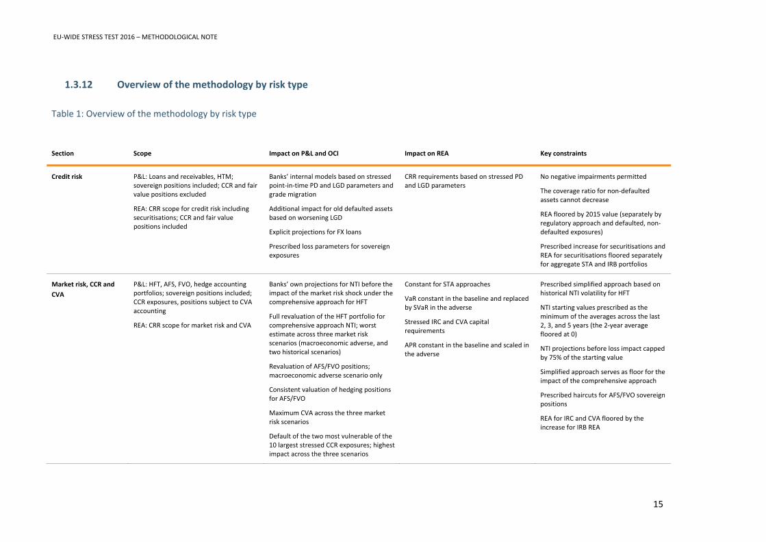
1.3.12 Overview of the methodology by risk type
Table 1: Overview of the methodology by risk type
Section Scope Impact on P&L and OCI Impact on REA Key constraints
Credit risk P&L: Loans and receivables, HTM; sovereign positions included; CCR and fair value positions excluded
REA: CRR scope for credit risk including securitisations; CCR and fair value positions included
Banks’ internal models based on stressed point‐in‐time PD and LGD parameters and grade migration
Additional impact for old defaulted assets based on worsening LGD
Explicit projections for FX loans
Prescribed loss parameters for sovereign exposures
CRR requirements based on stressed PD and LGD parameters
No negative impairments permitted
The coverage ratio for non‐defaulted assets cannot decrease
REA floored by 2015 value (separately by regulatory approach and defaulted, non‐defaulted exposures)
Prescribed increase for securitisations and REA for securitisations floored separately for aggregate STA and IRB portfolios
Market risk, CCR and
CVA
P&L: HFT, AFS, FVO, hedge accounting portfolios; sovereign positions included; CCR exposures, positions subject to CVA accounting
REA: CRR scope for market risk and CVA
Banks’ own projections for NTI before the impact of the market risk shock under the comprehensive approach for HFT
Full revaluation of the HFT portfolio for comprehensive approach NTI; worst estimate across three market risk scenarios (macroeconomic adverse, and two historical scenarios)
Revaluation of AFS/FVO positions; macroeconomic adverse scenario only
Consistent valuation of hedging positions for AFS/FVO
Maximum CVA across the three market risk scenarios
Default of the two most vulnerable of the 10 largest stressed CCR exposures; highest impact across the three scenarios
Constant for STA approaches
VaR constant in the baseline and replaced by SVaR in the adverse
Stressed IRC and CVA capital requirements
APR constant in the baseline and scaled in the adverse
Prescribed simplified approach based on historical NTI volatility for HFT
NTI starting values prescribed as the minimum of the averages across the last 2, 3, and 5 years (the 2‐year average floored at 0)
NTI projections before loss impact capped by 75% of the starting value
Simplified approach serves as floor for the impact of the comprehensive approach
Prescribed haircuts for AFS/FVO sovereign positions
REA for IRC and CVA floored by the increase for IRB REA
EU‐WIDE STRESS TEST 2016 – METHODOLOGICAL NOTE
16
Section Scope Impact on P&L and OCI Impact on REA Key constraints
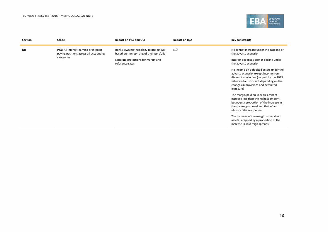
NII P&L: All interest‐earning or interest‐paying positions across all accounting categories
Banks’ own methodology to project NII based on the repricing of their portfolio
Separate projections for margin and reference rates
N/A NII cannot increase under the baseline or the adverse scenario
Interest expenses cannot decline under the adverse scenario
No income on defaulted assets under the adverse scenario, except income from discount unwinding (capped by the 2015 value and a constraint depending on the changes in provisions and defaulted exposure)
The margin paid on liabilities cannot increase less than the highest amount between a proportion of the increase in the sovereign spread and that of an idiosyncratic component
The increase of the margin on repriced assets is capped by a proportion of the increase in sovereign spreads
EU‐WIDE STRESS TEST 2016 – METHODOLOGICAL NOTE
17
Section Scope Impact on P&L and OCI Impact on REA Key constraints
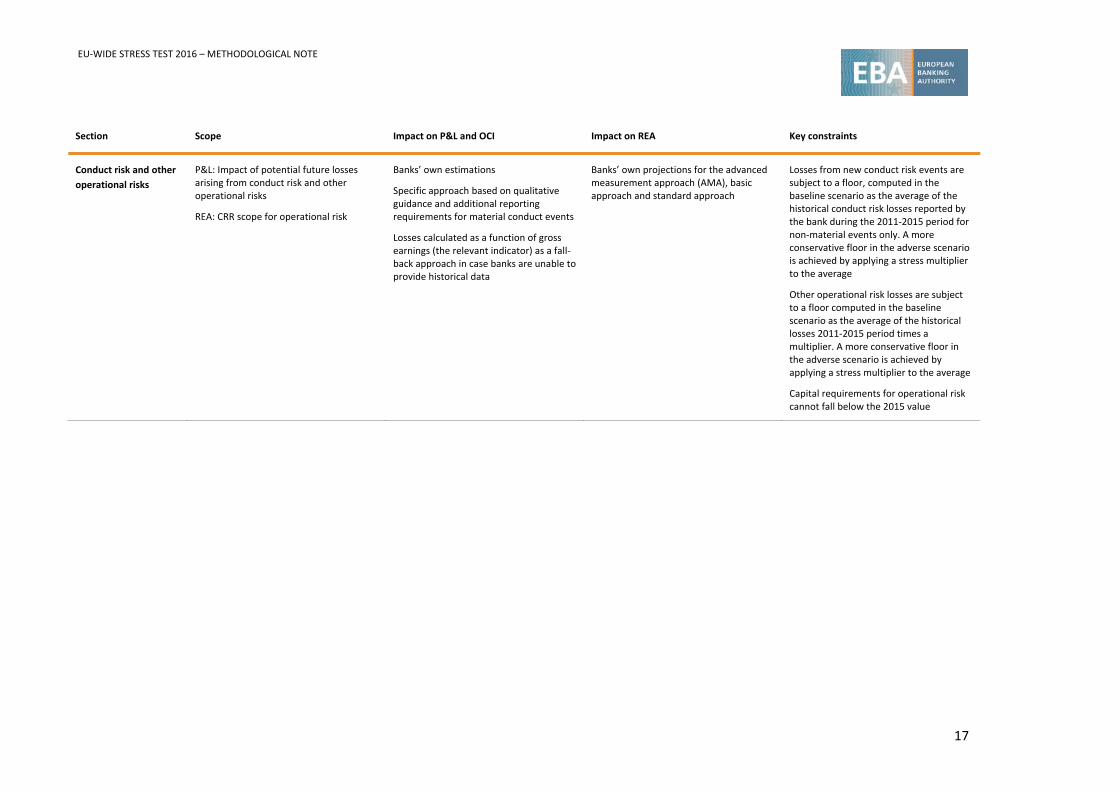
Conduct risk and other
operational risks
P&L: Impact of potential future losses arising from conduct risk and other operational risks
REA: CRR scope for operational risk
Banks’ own estimations
Specific approach based on qualitative guidance and additional reporting requirements for material conduct events
Losses calculated as a function of gross earnings (the relevant indicator) as a fall‐back approach in case banks are unable to provide historical data
Banks’ own projections for the advanced measurement approach (AMA), basic approach and standard approach
Losses from new conduct risk events are subject to a floor, computed in the baseline scenario as the average of the historical conduct risk losses reported by the bank during the 2011‐2015 period for non‐material events only. A more conservative floor in the adverse scenario is achieved by applying a stress multiplier to the average
Other operational risk losses are subject to a floor computed in the baseline scenario as the average of the historical losses 2011‐2015 period times a multiplier. A more conservative floor in the adverse scenario is achieved by applying a stress multiplier to the average
Capital requirements for operational risk cannot fall below the 2015 value
EU‐WIDE STRESS TEST 2016 – METHODOLOGICAL NOTE
18
Section Scope Impact on P&L and OCI Impact on REA Key constraints
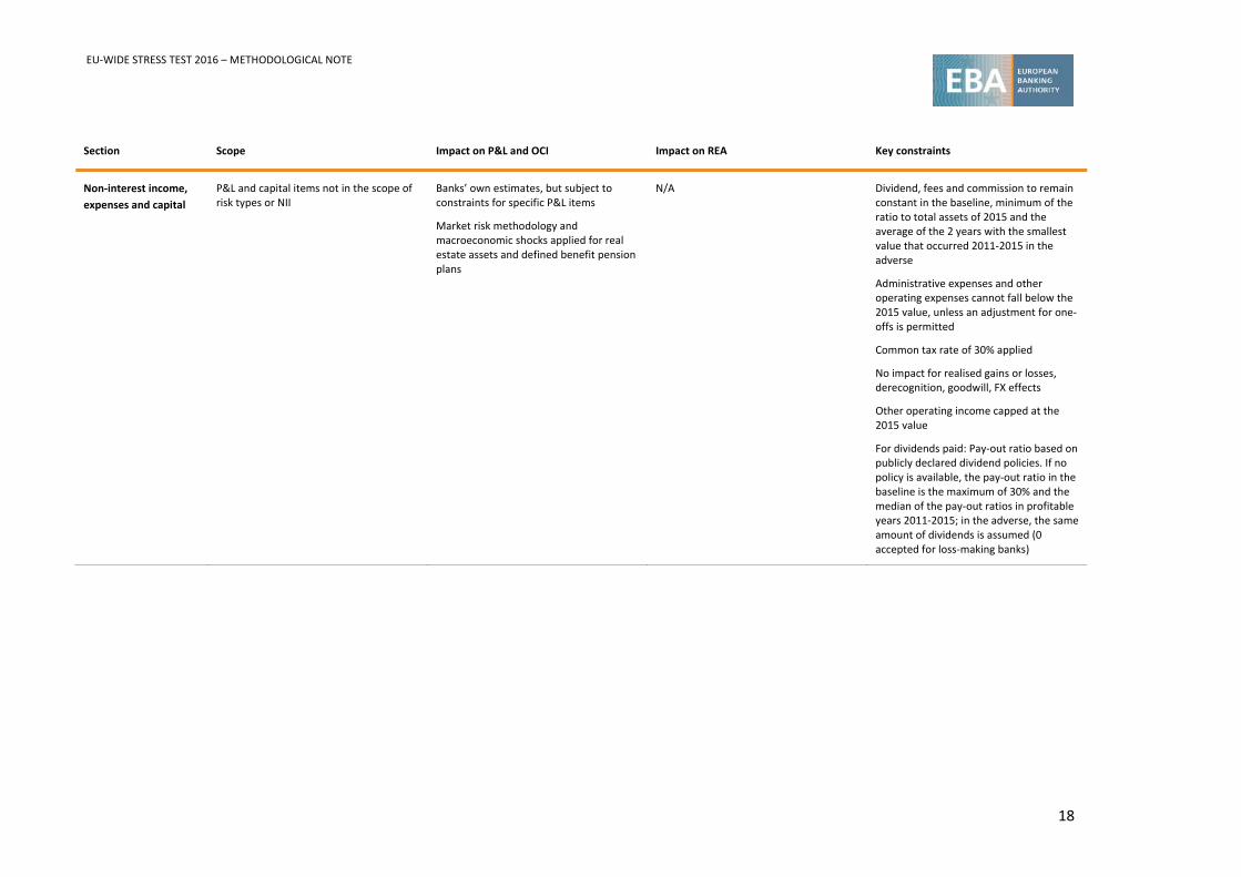
Non‐interest income,
expenses and capital
P&L and capital items not in the scope of risk types or NII
Banks’ own estimates, but subject to constraints for specific P&L items
Market risk methodology and macroeconomic shocks applied for real estate assets and defined benefit pension plans
N/A Dividend, fees and commission to remain constant in the baseline, minimum of the ratio to total assets of 2015 and the average of the 2 years with the smallest value that occurred 2011‐2015 in the adverse
Administrative expenses and other operating expenses cannot fall below the 2015 value, unless an adjustment for one‐offs is permitted
Common tax rate of 30% applied
No impact for realised gains or losses, derecognition, goodwill, FX effects
Other operating income capped at the 2015 value
For dividends paid: Pay‐out ratio based on publicly declared dividend policies. If no policy is available, the pay‐out ratio in the baseline is the maximum of 30% and the median of the pay‐out ratios in profitable years 2011‐2015; in the adverse, the same amount of dividends is assumed (0 accepted for loss‐making banks)
2016 EU‐WIDE STRESS TEST – METHODOLOGICAL NOTE
19
2. Credit risk
2.1 Overview
39. Banks are required to translate the macroeconomic scenarios into corresponding credit risk
impacts on both the capital available – i.e. via impairments and thus the P&L – and the REA for
positions exposed to risks stemming from the default of counterparties. Banks are requested
to make use of their models but are subject to a number of conservative constraints.
40. The estimation of impairments and translation to available capital requires the use of
statistical methods and includes the following main steps: (i) estimating starting values of the
risk parameters, (ii) estimating the impact of the scenarios on the risk parameters, and (iii)
computing impairment flows as the basis for provisions that affect the P&L.
41. For the estimation of REA, banks should adhere to regulatory requirements based on stressed
regulatory risk parameters.
42. For securitisation exposures, banks are requested to project impairments based on the risk
parameters of the underlying pool. For the estimation of REA, a fixed risk weight increase will
be applied to the different credit quality steps.
43. Banks’ projections are subject to the constraints summarised in Box 1.
Box 1: Summary of the constraints on banks’ projections of credit risk
No negative impairments for any given exposure are permitted for any year or scenario
(paragraphs 104 and 105).
The coverage ratio for non‐defaulted assets (i.e. ratio of provisions to exposure) cannot
decrease over the time horizon of the exercise (paragraph 104).
The end‐2015 level of REA serves as a floor for the total REA for non‐defaulted and defaulted
exposures in the baseline and the adverse scenarios. This floor must be applied separately to
overall aggregate IRB and STA portfolios (paragraph 115).
For securitisation exposures, the end‐2015 level of REA serves as a floor for the total risk
exposures separately for aggregate IRB and STA portfolios (paragraph 138).
2016 EU‐WIDE STRESS TEST – METHODOLOGICAL NOTE
20
2.2 Scope
44. For the estimation of the P&L impact, the scope of this section covers all counterparties (e.g.
sovereigns, institutions, financial and non‐financial firms and households) and all positions
(including on‐balance and off‐balance positions) exposed to risks stemming from the default of
a counterparty, except for exposures subject to CCR and fair value positions (HFT, AFS and
FVO), which are subject to the market risk approach for the estimation of the P&L effect (or
through capital, via OCI, for AFS) as stated in section 3.
45. Hedge accounting hedges related to positions within the scope of this section can only be
considered to the extent that they are already reflected in CRM or substitution effects as of
the reference date – i.e. there should be no additional offsetting impact from the hedging
instruments in hedge accounting portfolios measured at cost. These hedging instruments are
also not to be reported in market risk templates. Economic hedges are treated according to
the market risk methodology.
46. Conversely, the estimation of the REA follows the CRR/CRD definition of credit risk. Therefore,
exposures subject to CCR and fair value positions (AFS and FVO) are to be included.
47. Specific requirements for securitisation positions are separately covered in section 2.7.
48. The methodology described in this section also applies to the capital charge for IRC (see
paragraph 268).
2.3 High‐level assumptions and definitions
2.3.1 Definitions
49. Banks are required to apply consistent definitions for the following items.
50. The default definition to be used for the purpose of exposure classification (defaulted vs non‐
defaulted exposures) must be in line with the bank’s existing regulatory default recognition
procedures (Article 178 of the CRR).
51. Default flow (Def Flow) measures the amount of exposures that defaulted during a given year
out of those that were non‐defaulted at the start of the period. It must include all default
events that occur during a year. Exposures that defaulted several times in 2015 must be
reported once. The projected values will be computed based on the methodology stated in
this section.
52. Historical default rate (Def Rate) is defined as the flow of newly defaulted assets (Def Flow)
over exposure (Exp) at the beginning of the observation period. The default rate for 2015
would, therefore, be calculated as defaulted assets flow (in 2015) over performing exposure
(end 2014) for each asset class/country of the counterparty.
2016 EU‐WIDE STRESS TEST – METHODOLOGICAL NOTE
21
53. Exposure (Exp) is the non‐defaulted exposure after substitution effects and post credit
conversion factor (CCF). Exposure is the starting point for the impairment calculation.
Defaulted assets are reported separately:
For IRB portfolios, banks should use the definition of Column 110 (‘exposure value’) as
per COREP table CR IRB 1 as a starting point, and remove defaulted assets;
For STA portfolios, banks need to calculate a post CCF equivalent of Column 110 (net
exposure after CRM substitution effects pre‐conversion factors) as per COREP table
CR SA. Since provisions have already been deducted (Column 30 in CR SA), they need
to be added to the exposure. Defaulted assets must be reported in the respective
column ‘stock of defaulted exposures’.3
54. Share of non‐defaulted exposure of FX lending (Exp FX lending EUR, CHF) is the percentage of
non‐defaulted exposure (Exp) as defined above, where the currency of the credit facility is
different from the local currency of the borrower (see section 2.4.4).
55. Stock of defaulted exposures (Def Stock) refers to defaulted exposure according to the default
definition. As cures are not to be recognised for exposure projections, this is a cumulative
variable containing the initial stock of defaulted exposures (end 2015) plus the sum of default
flows of the previous projected year(s). For example, the stock of defaulted exposures in 2017
is the sum of the stock of defaulted exposures in 2015 plus defaulted flow in 2016 plus
defaulted flow in 2017.
56. Funded collateral (available) covers all funded collateral, including real estate property, that is
available to cover the exposure (Exp) or stock of defaulted exposures (Def Stock) as defined
above. Only CRR/CRD eligible collateral and only the bank’s share of collateral (in case
collateral is assigned to several debtors) is to be reported. No regulatory haircuts should be
applied. Banks are required to provide detailed information on how the collateral values have
been determined and how often appraisals are refreshed.
57. Funded collateral (capped) follows the definition of the available funded collateral (above) but
collateral has to be capped at the exposure level. This means that, at the exposure level,
collateral cannot be higher than the respective exposure.
58. The starting values of the stock of provisions (Prov Stock) must be the accounting figures as
of end 2015 in accordance with the accounting framework to which the reporting entity is
subject and in accordance with Article 34 and Article 110 of the CRR, as listed in columns 8, 9
and 10 of FINREP Table 7 (‘financial assets subject to impairment that are past due or
impaired’). It is split by stock of provisions for defaulted assets (Prov Stock Old) and stock of
provisions for non‐defaulted assets (Prov Stock non‐defaulted).
3 Defaulted assets are to be reported according to the nature of the counterparty.
2016 EU‐WIDE STRESS TEST – METHODOLOGICAL NOTE
22
59. The starting values of the gross impairment loss (Gross Imp Flow New) must be the
accounting flow figures as of end 2015, defined on the basis of ‘impairment on (non‐)financial
assets’ (FINREP, table 16.7, column 010; reported year‐to‐date – i.e. for the starting value
provisions that have been set aside in 2015). However, there are two important adjustments
to the FINREP figure: (i) the flow should be reported for newly defaulted assets only, and (ii)
the flow figures should also include direct write‐offs or charge‐offs of securities or other assets
whose book value is reduced without creating a provision. The guiding principle for this figure
is a point‐in‐time impairment flow, capturing all credit risk‐related adjustments, regardless of
whether those take the form of provisions or not. The impairment loss should correspond to
total impairments of newly defaulted assets and not only to the additional ones accumulated
during the year 2015 – i.e. the stock of impairments that existed at the beginning of the period
for these newly defaulted assets should be included.
60. Net impairment loss (Net Imp Flow New) is the gross impairment loss net of the release of
provisions from non‐defaulted assets caused by the new default flows. The projected values
will be computed based on the methodology stated in this section.
61. Cure rates are not observed values, but forecasted values affecting LGDpit estimation in 2015
and in the projected period across both scenarios. While the impact of cures for reducing
projected exposures in the default state should not be considered for the purpose of this
exercise, assumed cure rates are an important component of the LGD estimations. In doing so,
banks are required to model cure rates when estimating PDs and LGDs, and report them in the
templates CSV_CR_T0 and CSV_CR_SCEN according to the definitions below in a manner that
is consistent with the prescribed definition of default and LGD. In case a bank does not
explicitly calculate cure rates due to its methodological approach, it will be required to outline
its calculations of LGDpitOLD and LGDpitNEW in more detail in the accompanying note. The
following definitions apply:
CureNEW(t) is the component of the LGDNEW(t) calculation that corresponds to the
assumptions made for the cumulative proportion of newly defaulted exposures that
cure (through repayments) with zero loss in all years following year t;
CureOLD(t) is the component of the LGDOLD(t) calculation that corresponds to the
assumptions made for the cumulative proportion of existing defaulted exposures that
cure (through repayments) with zero loss in all years following year t. This naturally
depends on the characteristics of the loans that are already in default at time t.
62. Impairment loss for defaulted assets (Imp Flow Old) is a flow variable analogue to Gross Imp
Flow New, but defined for defaulted assets at the beginning of each period. In addition to
assumed cure rates, impairment loss for defaulted assets can be explained by other
components as the ones defined below. Banks are required to report these components in the
templates CSV_CR_T0 and CSV_CR_SCEN if their models allow for their computation. In case
banks are not able to calculate these components due to their methodological approach, they
2016 EU‐WIDE STRESS TEST – METHODOLOGICAL NOTE
23
will be required to outline their calculations of the impairment loss for defaulted assets in
more detail. The components to be reported are the following:
Impairment flow on old defaulted assets due to assumed changes in the loss given
loss (LGL), which corresponds to the change in future losses on those old defaulted
assets that will never cure. LGL is the part of the LGD that occurs if the exposure does
not cure. The probability of incurring this loss is equal to 1‐cure rate;
Impairment flow on old defaults due to subsequent defaults on the exposure
assumed to cure as implicit within the LGDpitOLD parameter.
63. Marginal impairment flow from FX lending (Imp Flow FX) refers to the aggregate marginal
contribution to the impairment flow from all FX exposures that meet the threshold (as defined
in paragraph 108). The projected values will be computed based on the methodology stated in
this section.
64. Historical loss rate (Loss Rate) is defined as gross impairment loss (Imp Flow New) over newly
defaulted assets (Def Flow).
65. Point‐in‐time risk parameters (PDpit, LGDpitNEW and LGDpitOLD) are the forward‐looking
projections of default rates and loss rates. The following requirements apply:
Since they are reported at a portfolio level, PDs must be exposure‐weighted averages,
and LGDs must be PD * exposure‐weighted averages;
PDpit and LGDpit must capture current trends in the business cycle. In contrast to
through‐the‐cycle parameters, they should not be business cycle neutral;
Contrary to regulatory parameters, PDpit and LGDpit are required for all portfolios,
including STA and Foundation IRB (F‐IRB);
LGDpit must be estimated for the stock of default (LGDpitOLD) and newly defaulted
assets (LGDpitNEW) in each period and must take into account collateral. Its evolution is
affected by PD/LGD grade migrations and such an effect must be addressed in the
estimation;
PDpit and LGDpit from FX lending for currencies as defined under exposure (Exp) must
be computed accordingly for the relevant asset classes in the respective currency,
subject to the threshold as defined in paragraph 108;
Although PDpit and LGDpit are reported together with default and impairment
amounts within the projected year, they must be considered to apply to exposures as
of the beginning of the year.
66. Grade migration refers to the change in the distribution of credit quality within a portfolio
over time. This includes both PD grades (corresponding to different probabilities of default)
2016 EU‐WIDE STRESS TEST – METHODOLOGICAL NOTE
24
and LGD grades (corresponding to LTVs, vintages, probabilities of curing or other factors
affecting the ultimate loss estimation for that exposure).
67. Migration contribution PDpit refers to the marginal contribution of rating grade migration and
is defined as the impact of PD grade migration – i.e. difference in percentage points between
the exposure‐weighted average PD of the non‐defaulted stock (Exp) pre‐migration vs post
migration under the same scenario. Only banks that calculate risk parameters at a rating class
level are requested to report this marginal contribution on an annual basis as memo items in
the templates based on the following components, in which migration contribution can be
broken down:
Default migration contribution (portfolio improvement effect): This effect measures
the impact of the migrations to default on the PDpit. All other rating migrations to
non‐defaulted rating categories are not considered. It is represented by the difference
between the portfolio level PDpit post default migration and portfolio level PDpit pre‐
migrations;
Migration effect to non‐defaulted rating grades: This effect captures pure rating
changes among non‐defaulted rating classes and complements the portfolio
improvement effect from above. It is expected that migrations to more risky rating
classes will exceed migrations to less risky rating classes as a result of the
deterioration of the macroeconomic scenario. It can be calculated as the PDpit post
non‐default migration minus the PDpit pre‐migrations.
68. Exposure value refers to exposure serving as the basis for computation of REA, according to
COREP definitions, as set out in Article 111 of the CRR (for the STA portfolio) and Articles 166
to 168 of the CRR (for the IRB portfolio).
69. Regulatory risk parameters (PDreg and LGDreg) refer to those parameters used for the
calculation of capital requirements for defaulted and non‐defaulted assets as prescribed by the
CRR.
70. ELreg is the EL based on regulatory risk parameters following the prescriptions of the CRR/CRD
for defaulted and non‐defaulted IRB exposures.
71. Level 3 assets, which must be reported in the securisation templates, refer to the assets
whose measurement is based on Level 3 inputs as defined in paragraph 86 of IFRS 13.
2.3.2 Static balance sheet assumption
72. According to the static balance sheet assumption, in line with section 1.3.8., banks are not
permitted to replace defaulted assets. Defaulted assets are moved into the defaulted assets
stock, reducing non‐defaulted assets and keeping the total exposure at a constant level.
2016 EU‐WIDE STRESS TEST – METHODOLOGICAL NOTE
25
Furthermore, for the purpose of calculating exposures, it is assumed that no cures, charge‐offs
or write‐offs should take place within the 3‐year horizon of the exercise.4
73. Within the credit risk framework, and for the purpose of calculating the credit REA, the initial
residual maturity is kept constant for all assets. This means that assets do not mature. For
example, a 10‐year bond with residual maturity of 5 years at the start of the exercise is
supposed to keep the same residual maturity of 5 years throughout the exercise. It should be
noted that the constant residual maturity applies, in particular, to the maturity factor used in
A‐IRB, but also to some provisions in STA, which allow for favourable risk weights for short‐
term exposures.
74. In addition fair value effects shall have not impact on exposure as well as on REA. This includes
changes in the FX rate.
2.3.3 Asset classes
75. For the purpose of this stress test, banks are required to report their exposures using the asset
classes specified below, which are based on the exposure classes for IRB and STA exposures in
the CRR (see Article 112 and 147 of the CRR) reported in COREP. Competent authorities can
require participating banks to report additional optional breakdowns for exposures where they
see significant risks. The additional breakdowns are marked as optional in Table 2 and Table 3.
76. Where exposures are transferred to other classes through credit risk mitigation techniques
(substitution approach), this transfer has to be performed in line with the asset classes given in
Table 2 and Table 3, and should be reported in asset classes after substitution. For the
remainder of this section, any definitions and calculations must be consistent with this
approach. For instance, default and loss rates, as well as PDs and LGD estimations, must be
calculated and estimated for portfolios after substitution.
77. The following tables contain the asset classes, including the additional optional asset classes
that should be used for both credit risk impairments and REA.
Table 2: Overview of IRB asset classes
IRB asset classes
Central banks and central governments Institutions Corporates
Corporates – Specialised lending Corporates – Specialised lending – Secured by real estate propertyCorporates – Specialised lending – Not secured by real estate property
Corporates – SME Corporates – SME – Secured by real estate property
4 This is not to be confused with the inclusion of assumptions on future cure rates and write‐offs in the generation of LGD parameters, which are implicitly assumed, where applicable.
2016 EU‐WIDE STRESS TEST – METHODOLOGICAL NOTE
26
IRB asset classes
Corporates – SME – Not secured by real estate propertyCorporates – Others
Corporates – Others – Secured by real estate propertyCorporates – Others – Not secured by real estate property
Retail Retail – Secured by real estate property
Retail – Secured by real estate property – SMERetail – Secured by real estate property – Non‐SME
(OPTIONAL) of which: Owner occupier(OPTIONAL) of which: Buy to let(OPTIONAL) of which: Other secured by real estate property
Retail – Qualifying revolving Retail – Other retail
Retail – Other retail – SME Retail – Other retail – Non‐SME
Equity Securitisation Other non‐credit obligation assets
Table 3: Overview of STA asset classes
STA asset classes
Central governments or central banks Regional governments or local authoritiesPublic sector entities Multilateral development banks International organisations Institutions Corporates
Corporate – SME Corporate – Non‐SME
Retail Retail – SME Retail – Non‐SME
Secured by mortgages on immovable propertySecured by mortgages on immovable property – SMESecured by mortgages on immovable property – Non‐SME
(OPTIONAL) of which: Owner occupier(OPTIONAL) of which: Buy to let(OPTIONAL) of which: Other secured by real estate property
Items associated with particularly high riskCovered bonds Claims on institutions and corporates with ST credit assessmentCollective investment undertakings Equity Securitisation Other exposures
2016 EU‐WIDE STRESS TEST – METHODOLOGICAL NOTE
27
2.3.4 Reporting requirements
78. Banks are requested to provide the credit risk information by regulatory approach for both the
total exposures and for the most relevant countries of counterparties to which the institutions
are exposed. The cells for the whole banking group contain the overall exposure of the group
towards all counterparties (i.e. it is not the sum of the country by country cells).
79. The country of the counterparty refers to the country of incorporation of the obligor. This
concept can be applied on an immediate‐obligor basis and on an ultimate‐risk basis. Hence,
credit risk mitigation (CRM) techniques can change the allocation of an exposure to a country.
80. The breakdown by country of the counterparty will be reported according to a minimum of:
i. 95% of the sum of exposure (Exp) and default stock (Def Stock), as defined in
section 2.3.1, reported in aggregate for three regulatory approaches (i.e. A‐IRB, F‐
IRB and STA);
ii. Top 10 countries in terms of aggregate sum of exposure (Exp) and default stock
(Def Stock), as stated above.
81. For example, a bank with 95% of its exposure concentrated in six countries will only fill data for
those six countries. By contrast, if the aggregate sum of exposure of a bank towards the largest
10 countries is below 95% of the total aggregate exposure, the bank will fill the template only
for the top 10 counterparty countries.
82. The cut‐off date to define the 95% of aggregate sum exposure and top 10 countries is
31 December 2015. The selected countries of the counterparties and the order must remain
constant for the three credit risk templates (CSV_CR_T0, CSV_CR_SCEN and CSV_CR_REA).
83. The same cut‐off date applies for the allocation of asset classes across the regulatory
approach. This means that a bank that applied the STA at the beginning of 2015 but the A‐IRB
approach at the end of 2015 is requested to report 2015 information (in template CSV_CR_T0)
in the A‐IRB section of the template.
2.4 Impact on P&L
2.4.1 Starting point‐in‐time risk parameters (a hierarchy of approaches)
84. The following paragraphs describe a hierarchy of methods that banks should adhere to when
they set the starting (unstressed) point‐in‐time risk parameters. As a general principle, banks
should resort to data from internal models rather than from accounting approximations:
For IRB portfolios, banks are required to base their estimation of starting level point‐
in‐time values on their approved internal parameter estimation models (refer to the
definitions of PDpit and LGDpit above);
2016 EU‐WIDE STRESS TEST – METHODOLOGICAL NOTE
28
For STA banks or IRB banks that cannot extract starting level point‐in‐time parameters
from their internal models for portfolios where there are no approved models in
place, banks should use non‐approved models to extract point‐in‐time parameters
provided those models are regularly used in internal risk management and stress
testing, and the competent authority is satisfied with using them for the purpose of
the EU‐wide stress test;
For portfolios where no appropriate internal models are in use for estimating the
starting level PDpit or LGDpit, banks are expected to approximate PDpit and LGDpit
starting values via default and loss rates (historically observed). While banks are
expected to present parameters reflective of both 2015 macroeconomic conditions
and the credit quality of the portfolios, in the calibration of point‐in‐time starting
parameters, the overarching objective is the parameter’s suitability for projection.
Therefore, banks are expected to consider factors that may lead to the observed
performance for 2015 being unrepresentative or unsuitable for a sufficiently
conservative projection or for small portfolios in which no default has been observed.
Only those adjustments of the historical values that result in a more conservative
starting point are permitted.
85. Irrespective of which approach is followed and the extent of the adjustments, banks are
required to provide a description of the methodology employed for deriving point‐in‐time
parameters for all portfolios. Banks are requested to apply the EBA terminology used in this
note, wherever applicable.
86. Participating banks will be subject to cross‐sectional comparisons of starting level point‐in‐
time parameters after the submission of the results, and might be asked to revise internal
figures if deemed not suitable for projections.
87. Historical values and starting point risk parameters shall be reported on the starting point
credit risk template (CSV_CR_T0).
2.4.2 Projected point‐in‐time parameters (a hierarchy of approaches)
88. Likewise, for the estimation of projected parameters, as a general principle, banks should use
models rather than resort to benchmarks to determine stressed PDpit and LGDpit parameters
(under both the baseline and the adverse scenario). However, banks’ models will be assessed
by competent authorities against minimum standards in terms of econometric soundness and
responsiveness of the risk parameters to ensure the model specification results in a prudent
outcome.
89. For portfolios where no appropriate satellite models are available for estimating the stressed
PDpit or LGDpit, banks are expected to base their evolution on the benchmark parameters
provided by the ECB. They should apply them at portfolio level, not at rating class level.
2016 EU‐WIDE STRESS TEST – METHODOLOGICAL NOTE
29
90. Irrespective of the approach, the ECB benchmark parameters will serve as an important
benchmark to gauge internal PDpit and LGDpit parameter estimates in the baseline as well as
in the adverse scenario as described in the following paragraphs. Moreover, banks will be
subject to cross‐sectional comparisons after the submission of the results, and might be asked
to revise internal figures if deemed overly optimistic.
91. If banks’ models allow for the estimation of the relationship between point‐in‐time
parameters and the macroeconomic variables at a rating class level, institutions shall employ a
rating transition matrix‐based approach, considering the effects of PD/LGD grade migration on
the level of default and impairments projected in the stress test horizon for the given
scenarios. In this case, banks are required to calculate point‐in‐time transition matrices.
Transition matrices must satisfy the following minimum criteria:
The PD/LGD for each grade is adjusted appropriately to reflect the scenario;
This probability of moving from one grade to another is appropriately adjusted according to
the scenario.
92. Banks projecting at a rating class level are requested to report this grade migration
contribution. Reported portfolio level aggregate parameters (PDs and LGDs) are rating class
volume‐weighted average at the starting point and along the scenario horizon. Banks are
required to explain how they have accounted for the effects of grade migration in their
estimations.
93. The distribution of exposures across buckets (which are used to calculate the corresponding
aggregate parameters) are the result of multiplying the distribution of exposures at the end of
the previous year by the point‐in‐time migration matrix. Box 2 provides an example of the
effect of a grade migration matrix.
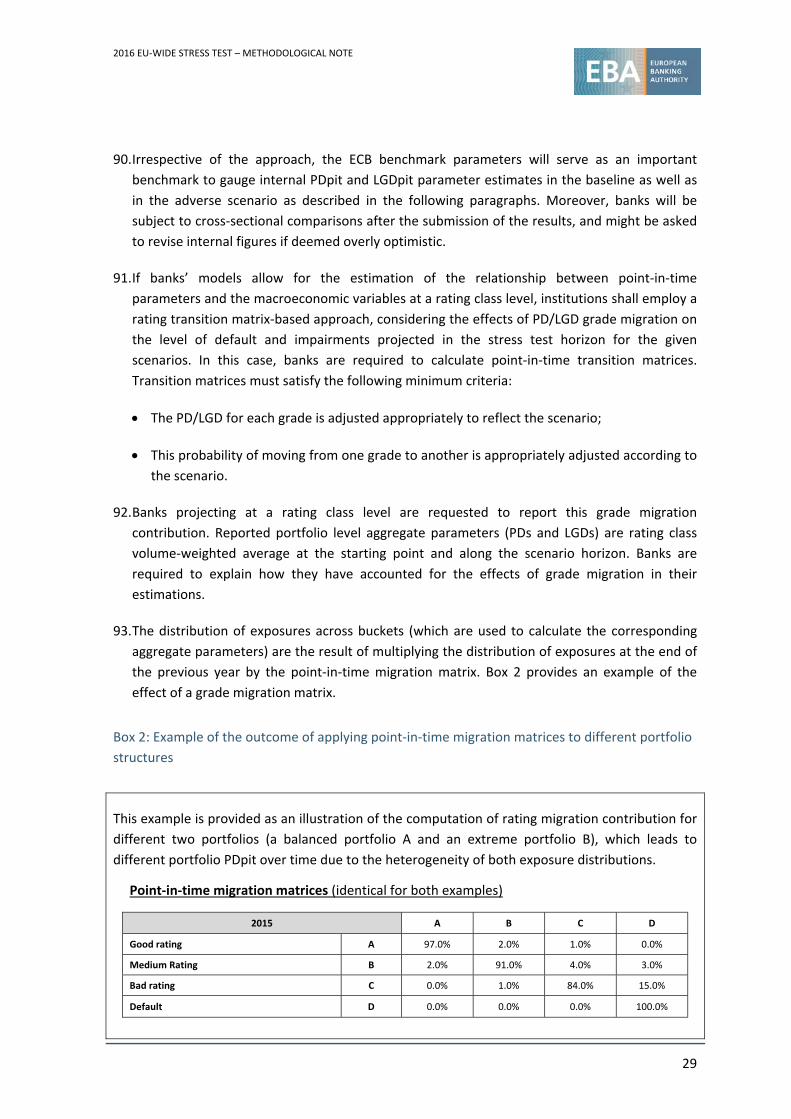
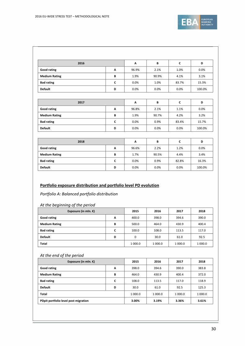
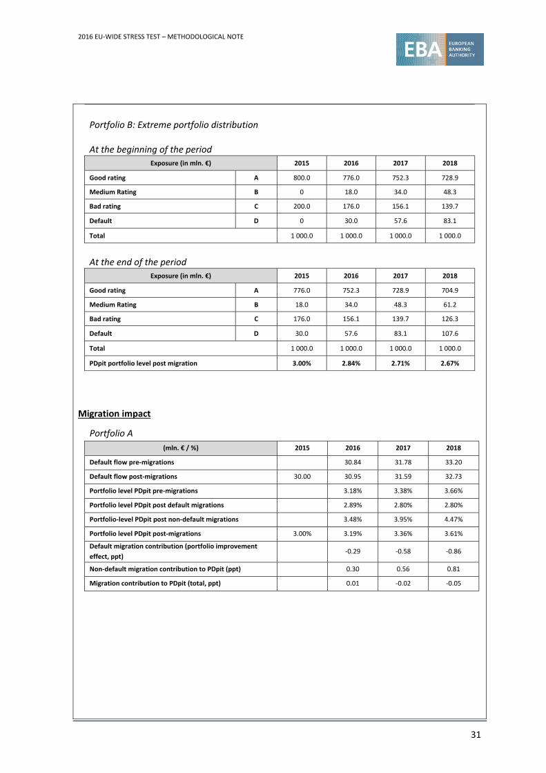
Box 2: Example of the outcome of applying point‐in‐time migration matrices to different portfolio
structures
This example is provided as an illustration of the computation of rating migration contribution for
different two portfolios (a balanced portfolio A and an extreme portfolio B), which leads to
different portfolio PDpit over time due to the heterogeneity of both exposure distributions.
Point‐in‐time migration matrices (identical for both examples)
2015 A B C D
Good rating A 97.0% 2.0% 1.0% 0.0%
Medium Rating B 2.0% 91.0% 4.0% 3.0%
Bad rating C 0.0% 1.0% 84.0% 15.0%
Default D 0.0% 0.0% 0.0% 100.0%
2016 EU‐WIDE STRESS TEST – METHODOLOGICAL NOTE
30
2016 A B C D
Good rating A 96.9% 2.1% 1.0% 0.0%
Medium Rating B 1.9% 90.9% 4.1% 3.1%
Bad rating C 0.0% 1.0% 83.7% 15.3%
Default D 0.0% 0.0% 0.0% 100.0%
2017 A B C D
Good rating A 96.8% 2.1% 1.1% 0.0%
Medium Rating B 1.9% 90.7% 4.2% 3.2%
Bad rating C 0.0% 0.9% 83.4% 15.7%
Default D 0.0% 0.0% 0.0% 100.0%
2018 A B C D
Good rating A 96.6% 2.2% 1.2% 0.0%
Medium Rating B 1.7% 90.5% 4.4% 3.4%
Bad rating C 0.0% 0.9% 82.8% 16.3%
Default D 0.0% 0.0% 0.0% 100.0%
Portfolio exposure distribution and portfolio level PD evolution
Portfolio A: Balanced portfolio distribution At the beginning of the period
Exposure (in mln. €) 2015 2016 2017 2018
Good rating A 400.0 398.0 394.6 390.0
Medium Rating B 500.0 464.0 430.9 400.4
Bad rating C 100.0 108.0 113.5 117.0
Default D 0 30.0 61.0 92.5
Total 1 000.0 1 000.0 1 000.0 1 000.0
At the end of the period
Exposure (in mln. €) 2015 2016 2017 2018
Good rating A 398.0 394.6 390.0 383.8
Medium Rating B 464.0 430.9 400.4 372.0
Bad rating C 108.0 113.5 117.0 118.9
Default D 30.0 61.0 92.5 125.3
Total 1 000.0 1 000.0 1 000.0 1 000.0
PDpit portfolio level post migration 3.00% 3.19% 3.36% 3.61%
2016 EU‐WIDE STRESS TEST – METHODOLOGICAL NOTE
31
Portfolio B: Extreme portfolio distribution At the beginning of the period
Exposure (in mln. €) 2015 2016 2017 2018
Good rating A 800.0 776.0 752.3 728.9
Medium Rating B 0 18.0 34.0 48.3
Bad rating C 200.0 176.0 156.1 139.7
Default D 0 30.0 57.6 83.1
Total 1 000.0 1 000.0 1 000.0 1 000.0
At the end of the period
Exposure (in mln. €) 2015 2016 2017 2018
Good rating A 776.0 752.3 728.9 704.9
Medium Rating B 18.0 34.0 48.3 61.2
Bad rating C 176.0 156.1 139.7 126.3
Default D 30.0 57.6 83.1 107.6
Total 1 000.0 1 000.0 1 000.0 1 000.0
PDpit portfolio level post migration 3.00% 2.84% 2.71% 2.67%
Migration impact
Portfolio A
(mln. € / %) 2015 2016 2017 2018
Default flow pre‐migrations 30.84 31.78 33.20
Default flow post‐migrations 30.00 30.95 31.59 32.73
Portfolio level PDpit pre‐migrations 3.18% 3.38% 3.66%
Portfolio level PDpit post default migrations 2.89% 2.80% 2.80%
Portfolio‐level PDpit post non‐default migrations 3.48% 3.95% 4.47%
Portfolio level PDpit post‐migrations 3.00% 3.19% 3.36% 3.61%
Default migration contribution (portfolio improvement
effect, ppt) ‐0.29 ‐0.58 ‐0.86
Non‐default migration contribution to PDpit (ppt) 0.30 0.56 0.81
Migration contribution to PDpit (total, ppt) 0.01 ‐0.02 ‐0.05
2016 EU‐WIDE STRESS TEST – METHODOLOGICAL NOTE
32
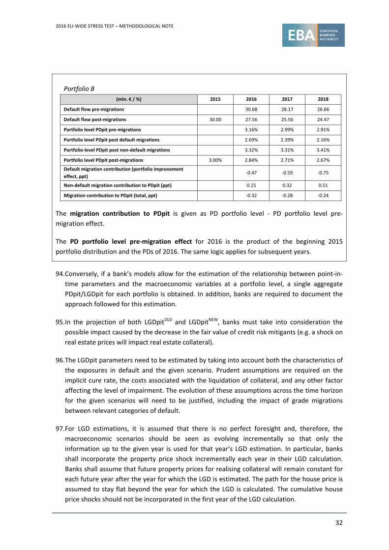
Portfolio B
(mln. € / %) 2015 2016 2017 2018
Default flow pre‐migrations 30.68 28.17 26.66
Default flow post‐migrations 30.00 27.56 25.56 24.47
Portfolio level PDpit pre‐migrations 3.16% 2.99% 2.91%
Portfolio level PDpit post default migrations 2.69% 2.39% 2.16%
Portfolio‐level PDpit post non‐default migrations 3.32% 3.31% 3.41%
Portfolio level PDpit post‐migrations 3.00% 2.84% 2.71% 2.67%
Default migration contribution (portfolio improvement
effect, ppt) ‐0.47 ‐0.59 ‐0.75
Non‐default migration contribution to PDpit (ppt) 0.15 0.32 0.51
Migration contribution to PDpit (total, ppt) ‐0.32 ‐0.28 ‐0.24
The migration contribution to PDpit is given as PD portfolio level ‐ PD portfolio level pre‐
migration effect.
The PD portfolio level pre‐migration effect for 2016 is the product of the beginning 2015
portfolio distribution and the PDs of 2016. The same logic applies for subsequent years.
94. Conversely, if a bank’s models allow for the estimation of the relationship between point‐in‐
time parameters and the macroeconomic variables at a portfolio level, a single aggregate
PDpit/LGDpit for each portfolio is obtained. In addition, banks are required to document the
approach followed for this estimation.
95. In the projection of both LGDpitOLD and LGDpitNEW, banks must take into consideration the
possible impact caused by the decrease in the fair value of credit risk mitigants (e.g. a shock on
real estate prices will impact real estate collateral).
96. The LGDpit parameters need to be estimated by taking into account both the characteristics of
the exposures in default and the given scenario. Prudent assumptions are required on the
implicit cure rate, the costs associated with the liquidation of collateral, and any other factor
affecting the level of impairment. The evolution of these assumptions across the time horizon
for the given scenarios will need to be justified, including the impact of grade migrations
between relevant categories of default.
97. For LGD estimations, it is assumed that there is no perfect foresight and, therefore, the
macroeconomic scenarios should be seen as evolving incrementally so that only the
information up to the given year is used for that year’s LGD estimation. In particular, banks
shall incorporate the property price shock incrementally each year in their LGD calculation.
Banks shall assume that future property prices for realising collateral will remain constant for
each future year after the year for which the LGD is estimated. The path for the house price is
assumed to stay flat beyond the year for which the LGD is calculated. The cumulative house
price shocks should not be incorporated in the first year of the LGD calculation.
2016 EU‐WIDE STRESS TEST – METHODOLOGICAL NOTE
33
98. In order to assess the projected LGD parameters, historical LGD parameters for 2015 are
requested as memorandum items. In addition to the LGDs based on the coverage ratio, banks
must also provide, on the starting point credit risk template (CSV_CR_T0), the LGDNEW and
LGDOLD under the above assumption of holding the 2015 macroeconomic conditions constant.
99. Projected risk parameters shall be reported on the credit risk scenario template (CSV_CR_
SCEN).
2.4.3 Calculation of defaulted assets and impairments
100. The evolution of the PDpit and LGDpit as described in the previous section must be applied
to the computation of the defaulted asset flow and the impairment flow on defaulted assets.
101. Consistent with the static balance sheet assumption (see section 2.3.2), non‐defaulted
credit exposure only changes due to the yearly default flows. Market value fluctuations have
no impact on the exposure and, in particular, cannot decrease the exposure.
102. The impairment losses for new and old defaulted assets computed (as described in the
following sections) will be reported in the P&L as impairment of financial assets other than
instruments designated at fair value through P&L.
103. Projected defaulted assets and impairment flows shall be reported on the credit risk
scenario template (CSV_CR_SCEN).
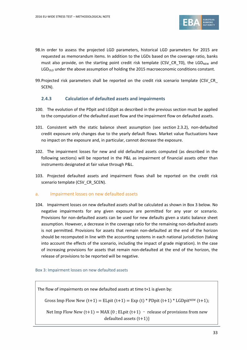
a. Impairment losses on new defaulted assets
104. Impairment losses on new defaulted assets shall be calculated as shown in Box 3 below. No
negative impairments for any given exposure are permitted for any year or scenario.
Provisions for non‐defaulted assets can be used for new defaults given a static balance sheet
assumption. However, a decrease in the coverage ratio for the remaining non‐defaulted assets
is not permitted. Provisions for assets that remain non‐defaulted at the end of the horizon
should be recomputed in line with the accounting systems in each national jurisdiction (taking
into account the effects of the scenario, including the impact of grade migration). In the case
of increasing provisions for assets that remain non‐defaulted at the end of the horizon, the
release of provisions to be reported will be negative.
Box 3: Impairment losses on new defaulted assets
The flow of impairments on new defaulted assets at time t+1 is given by:
GrossImpFlowNew t 1 ELpit t 1 Exp t *PDpit t 1 *LGDpitNEW t 1 ;
NetImpFlowNew t 1 MAX 0;ELpit t 1 – releaseofprovisionsfromnewdefaultedassets t 1
2016 EU‐WIDE STRESS TEST – METHODOLOGICAL NOTE
34
MAX 0;Exp t *PDpit t 1 *LGDpitNEW t 1 –α*ProvStocknon‐defaulted t .
Where:
ELpit t 1 andreleaseofprovisionsfromnewdefaultedassets t 1 aredefinedbytheformulasabove;
α is the share of Prov Stock non‐defaulted t which is linked to initially non‐defaulted assets at t, and which enter into default status at t+1. At a maximum, α can be equal to the
share of non‐defaulted assets at t, which enter into default at t+1 – i.e. α PDpit t 1 ;
ProvStocknon‐defaulted t is the stock of provisions against non‐defaulted assets at t;
PDpit t 1 and LGDpit t 1 both refer to the period from t to t+1 (year t+1).
This then leads to the following non‐defaulted exposure at time t+1:
Exp t 1 Exp t – Exp t *PDpit t 1 .
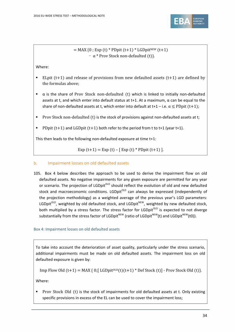
b. Impairment losses on old defaulted assets
105. Box 4 below describes the approach to be used to derive the impairment flow on old
defaulted assets. No negative impairments for any given exposure are permitted for any year
or scenario. The projection of LGDpitOLD should reflect the evolution of old and new defaulted
stock and macroeconomic conditions. LGDpitOLD can always be expressed (independently of
the projection methodology) as a weighted average of the previous year’s LGD parameters:
LGDpitOLD, weighted by old defaulted stock, and LGDpitNEW, weighted by new defaulted stock,
both multiplied by a stress factor. The stress factor for LGDpitOLD is expected to not diverge
substantially from the stress factor of LGDpitNEW (ratio of LGDpitNEW(t) and LGDpitNEW(t0)).
Box 4: Impairment losses on old defaulted assets
To take into account the deterioration of asset quality, particularly under the stress scenario,
additional impairments must be made on old defaulted assets. The impairment loss on old
defaulted exposure is given by:
ImpFlowOld t 1 MAX 0; LGDpitOLD t t 1 *DefStock t ‐ProvStockOld t .
Where:
Prov Stock Old t is the stock of impairments for old defaulted assets at t. Only existing
specific provisions in excess of the EL can be used to cover the impairment loss;
2016 EU‐WIDE STRESS TEST – METHODOLOGICAL NOTE
35
LGDpitOLD t t 1 is the LGD estimated in t+1 for the stock (at t) of old defaulted assets.
c. Impairment losses on sovereign exposures
106. Banks are requested to estimate default and impairment flows for sovereign positions
recorded as loans and receivables, or HTM investments according to the macroeconomic
baseline and adverse scenario. This covers positions whose exposure (Exp) is reported under
the categories ‘central banks and central governments’ for IRB portfolios, as well as ‘central
governments or central banks’ and ‘regional governments or local authorities’ for STA
portfolios. For exposures to central banks contained in the above IRB and STA portfolios zero
loss rates are to be applied under the baseline and the adverse scenario. Fair value positions
(i.e. AFS and FVO) will be subject to the market risk approach.
107. In order to compute these impairment flows, banks will be provided with a set of stressed
probability of default and loss given default parameters developed by the ECB for a selection
of countries. The application of these parameters is mandatory for all banks.
2.4.4 FX lending
108. Banks with significant foreign currency exposure are requested to take into account the
altered creditworthiness of their respective obligors, given the FX evolution under the baseline
and adverse scenario. In particular, banks are requested to evaluate this impact for exposures
denominated in a currency other than the local currency of the borrower at asset class level
for each country of counterparty if the total share of exposures in foreign currencies is above
the thresholds described in Table 4 and Table 6 below.
109. This effect should be accounted for in case of any depreciation of the local currency vis‐à‐
vis foreign currency debt (from the obligor’s perspective) included in the macroeconomic
scenarios. While all banks have to report the share of FX lending according to the requested FX
breakdown on the starting point credit risk template (CSV_CR_T0), only the latter (i.e. those
that meet the threshold as indicated in Table 4 and Table 6) have to calculate the additional
impact on the credit risk templates (CSV_CR_T0 and CSV_CR_SCEN). It should be noted that
exposures in euros are only to be reported in case the euro is not the local currency (e.g. an
exposure in euros in the Czech Republic has to be reported, while exposures in euros in
Slovakia do not have to be reported).
110. The marginal impact from the risk emanating from FX lending exposure has to cover both
PDs and LGDs. For PDs, the impact should be based on satellite models that link the
macroeconomic scenario to the PDpit. For the LGD, the impact should be based on an add‐on
for the LTV ratio in the case of collateralised exposures, while, in the case of uncollateralised
exposures, banks should apply the appropriate FX add‐on based on relevant historical
information.
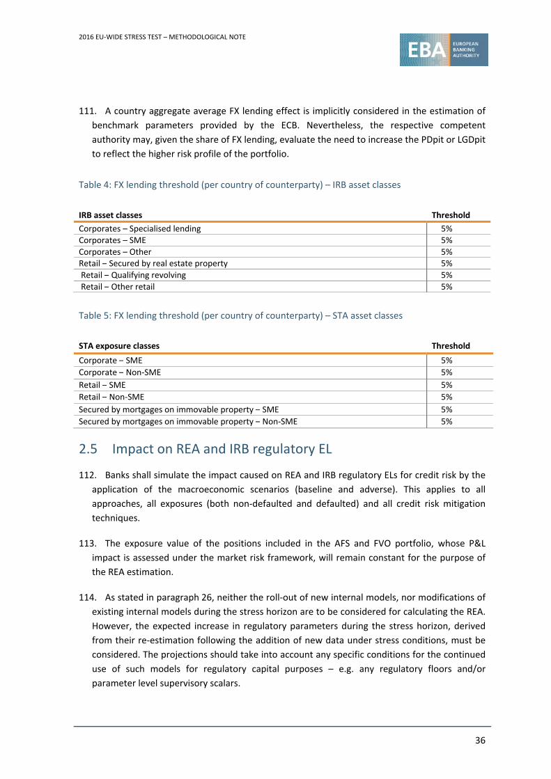
2016 EU‐WIDE STRESS TEST – METHODOLOGICAL NOTE
36
111. A country aggregate average FX lending effect is implicitly considered in the estimation of
benchmark parameters provided by the ECB. Nevertheless, the respective competent
authority may, given the share of FX lending, evaluate the need to increase the PDpit or LGDpit
to reflect the higher risk profile of the portfolio.
Table 4: FX lending threshold (per country of counterparty) – IRB asset classes
IRB asset classes Threshold
Corporates – Specialised lending 5% Corporates – SME 5%
Corporates – Other 5% Retail – Secured by real estate property 5%
Retail – Qualifying revolving 5%
Retail – Other retail 5%
Table 5: FX lending threshold (per country of counterparty) – STA asset classes
STA exposure classes Threshold
Corporate – SME 5%
Corporate – Non‐SME 5%
Retail – SME 5%
Retail – Non‐SME 5%
Secured by mortgages on immovable property – SME 5%
Secured by mortgages on immovable property – Non‐SME 5%
2.5 Impact on REA and IRB regulatory EL
112. Banks shall simulate the impact caused on REA and IRB regulatory ELs for credit risk by the
application of the macroeconomic scenarios (baseline and adverse). This applies to all
approaches, all exposures (both non‐defaulted and defaulted) and all credit risk mitigation
techniques.
113. The exposure value of the positions included in the AFS and FVO portfolio, whose P&L
impact is assessed under the market risk framework, will remain constant for the purpose of
the REA estimation.
114. As stated in paragraph 26, neither the roll‐out of new internal models, nor modifications of
existing internal models during the stress horizon are to be considered for calculating the REA.
However, the expected increase in regulatory parameters during the stress horizon, derived
from their re‐estimation following the addition of new data under stress conditions, must be
considered. The projections should take into account any specific conditions for the continued
use of such models for regulatory capital purposes – e.g. any regulatory floors and/or
parameter level supervisory scalars.
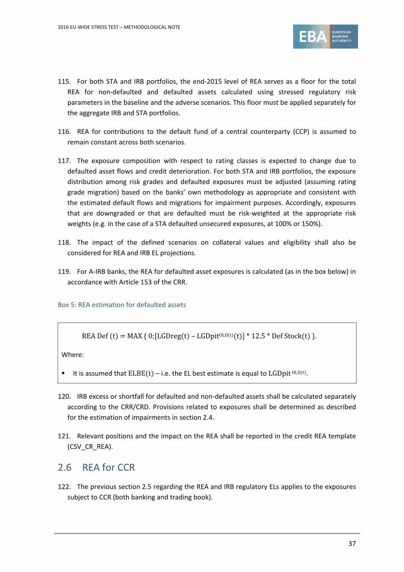
2016 EU‐WIDE STRESS TEST – METHODOLOGICAL NOTE
37
115. For both STA and IRB portfolios, the end‐2015 level of REA serves as a floor for the total
REA for non‐defaulted and defaulted assets calculated using stressed regulatory risk
parameters in the baseline and the adverse scenarios. This floor must be applied separately for
the aggregate IRB and STA portfolios.
116. REA for contributions to the default fund of a central counterparty (CCP) is assumed to
remain constant across both scenarios.
117. The exposure composition with respect to rating classes is expected to change due to
defaulted asset flows and credit deterioration. For both STA and IRB portfolios, the exposure
distribution among risk grades and defaulted exposures must be adjusted (assuming rating
grade migration) based on the banks’ own methodology as appropriate and consistent with
the estimated default flows and migrations for impairment purposes. Accordingly, exposures
that are downgraded or that are defaulted must be risk‐weighted at the appropriate risk
weights (e.g. in the case of a STA defaulted unsecured exposures, at 100% or 150%).
118. The impact of the defined scenarios on collateral values and eligibility shall also be
considered for REA and IRB EL projections.
119. For A‐IRB banks, the REA for defaulted asset exposures is calculated (as in the box below) in
accordance with Article 153 of the CRR.
Box 5: REA estimation for defaulted assets
READef t MAX 0; LGDreg t – LGDpitOLD t t *12.5*DefStock t .
Where:
It is assumed that ELBE t – i.e. the EL best estimate is equal to LGDpitOLD t .
120. IRB excess or shortfall for defaulted and non‐defaulted assets shall be calculated separately
according to the CRR/CRD. Provisions related to exposures shall be determined as described
for the estimation of impairments in section 2.4.
121. Relevant positions and the impact on the REA shall be reported in the credit REA template
(CSV_CR_REA).
2.6 REA for CCR
122. The previous section 2.5 regarding the REA and IRB regulatory ELs applies to the exposures
subject to CCR (both banking and trading book).
2016 EU‐WIDE STRESS TEST – METHODOLOGICAL NOTE
38
123. For the purpose of calculating the REA for CCR, regulatory exposures relating to CCR will be
reported using the appropriate template (CSV_CR_REA) and asset classes listed in Table 2 and
Table 3 only for this purpose.
124. CCR regulatory exposure will remain constant and will not be affected by the impact of
baseline and adverse market risk scenarios nor by any offset for increased accounting CVA in
the scenarios (as set out in Article 273(6) of the CRR). In particular, as set out in section 2.5,
stressed regulatory PD and LGD parameters (PDreg and LGDreg) shall be applied to these
constant CCR regulatory exposures for the calculation of stressed REA for CCR.
2.7 Securitisation exposures
125. All exposures subject to Chapter 5 of the CRR (traditional and synthetic, re‐securitisations,
as well as liquidity lines on securitisation transactions) are included in the scope of this section.
126. Originator positions where no SRT has taken place are to be treated under the credit risk
methodology, and should be reported accordingly in the credit risk templates. In particular this
holds for originator and investor exposures to securitisations issued or guaranteed by
international organisations, multilateral development banks, governments, or government
agencies, where firms are subject to the credit risk of these institutions rather than the credit
risk of the underlying exposures. Securitisation exposures within correlation trading portfolios
are covered by the market risk methodology and must be reported within market risk
templates.
127. In line with section 2.3.2, the static balance sheet assumption should be applied by keeping
the outstanding balance of all securitisation exposures unchanged throughout the time
horizon of the stress test. Fair value changes should not have an impact on the exposure
amount and the REA calculation for the application of the credit risk methodology.
128. For the computation of the P&L impact, banks are required to estimate the amount of
impairments for securitisation exposures that are not subject to mark‐to‐market valuation,
taking into account the features of the baseline and adverse macroeconomic scenarios. AFS
and FVO are thus excluded from the calculation of impairments. The forecasted impairments
should take into consideration impairments already considered in prior periods, and
incremental impairments for each period must be added, and reported appropriately, in the
securitisation templates. For each individual security, the underlying pool’s credit and
prepayment models must be stressed under the different scenarios to produce consistent
impairment estimates. Estimated impairments should take into consideration the impact of
credit enhancement and other structural features when applying the credit risk methodology.
Banks are required to outline their calculations in an accompanying document.
129. For securitisation exposures subject to mark‐to‐market valuation (i.e. AFS, FVO, and HFT),
banks are required to estimate the P&L impact via the mark‐to‐market loss incurred as a result
of the impact of the scenarios according to the market risk methodology (see section 3).
2016 EU‐WIDE STRESS TEST – METHODOLOGICAL NOTE
39
130. For the estimation of the REA, the stress is applied to the securitisation positions both in
banking and the trading book (within the scope of this section) according to their regulatory
treatment.
131. For regulatory approaches based on risk weights (i.e. the STA and the IRB method – except
exposures under the supervisory formula), a fixed risk weight increase will be applied to the
different credit quality steps as of 31 December 2015 by substituting the original risk weights
with predefined increased ones. The increased risk weights reflect the effect on REA of the
potential rating migration of the positions. The impact will be shown separately on the
securitisation templates according to regulatory approach (CSV_CR_SEC_STA,
CSV_CR_SEC_IRB).
132. For this purpose, the securitisation positions are allocated to the three different
securitisation categories for which the increase in REA is prescribed: low, medium and high
risk. The differentiation is dependent on the structure or asset class of the transaction,
regional differentiation, the credit quality of the position and the expected sensitivity to the
macroeconomic scenario. The classification is based on an analysis of the migration volatility of
different products and their origin, where a higher migration probability indicates a higher risk.
The risk categories and allocation of products are the following:
Risk bucket 1 (low risk): ABCP, EMEA RMBS, EMEA ABS, Americas ABS;
Risk bucket 2 (medium risk): EMEA CMBS, EMEA CDO, Americas CMBS;
Risk bucket 3 (high risk): Americas RMBS, Americas CDO and all other positions, including
re‐securitisations.
133. Banks are asked to supply information on the IRB and STA exposure per defined risk
buckets. For this purpose, the securitisation positions should be reported in the securitisation
templates by credit quality step, securitisation vs re‐securitisation, REA calculation approach,
and seniority and granularity based on corresponding CRR definitions (e.g. Articles 255, 251,
259, 261 and 262 of the CRR).
134. Banks should estimate the amount of impairments before the calculation of risk‐weighted
assets for securitisation positions. Impairments estimated for the computation of the P&L
impact will be taken into account in accordance with CRR Article 246(1) and Article 266(2).
Therefore, for exposures under the STA approach, impairments will be subtracted from the
exposure to be risk‐weighted. For exposures under the IRB approach, risk weights must be
applied on the full exposure (gross of impairments) and then subtract 12.5 times the
impairment provisions. Impairment estimates for securitisations shall be reported in the
securitisation summary template (CSV_CR_SEC_SUM).
135. When external ratings are not available and the banks use the Internal Assessment
Approach (IAA) for REA calculation purposes, these securitisation positions should be stressed
according to what is stated in the previous paragraphs. Each securitisation position should be
2016 EU‐WIDE STRESS TEST – METHODOLOGICAL NOTE
40
assigned the respective credit quality step whose average risk weight is the closest to the one
in the considered securitisation contract. As REA for positions under IAA are computed
differently for the projected period compared to the starting point, IRB REA for 2015, contrary
to projected values, the 2015 starting value shall be explicitly reported in the securitisation
summary template (CSV_CR_SEC_SUM).
136. When the banks use the supervisory formula approach (SFA) for REA calculation purposes,
they shall apply the stress factors for unsecuritised corporate or retail exposures to the risk
components (PD, LGD) of the asset pool in the respective exposure class. In this case, as a
precondition, the IRB banks will have to demonstrate to the respective competent authority
that the internal methods can be adjusted in a way that is consistent with the scenarios.
Beyond the requested data in the relevant template, banks are required to outline their
calculations in the accompanying document, reporting all their driving parameters.
137. The securitisation positions under the IRB SFA and other positions (look through) shall be
reported separately (CSV_CR_SEC_IRB_SF, CSV_CR_SEC_Other).
138. For both the STA and IRB portfolios, the end‐2015 level of REA serves as a floor for the total
REA calculated under the baseline and the adverse scenarios. This floor must be applied
separately for aggregate IRB and STA portfolios.
2016 EU‐WIDE STRESS TEST – METHODOLOGICAL NOTE
41
3. Market risk, CCR losses and CVA
3.1 Overview
139. The impact of market risk on AFS and FVO positions is to be assessed via a full revaluation,
after applying a common set of stressed market parameters consistent with the
macroeconomic adverse scenario. Prescribed haircuts have to be applied for sovereign
positions in these portfolios.
140. Regarding the HFT category, two different approaches shall be distinguished:
The comprehensive approach relies on a full revaluation for the macroeconomic
adverse and two historical scenarios, and is to be used by banks with internal models
or a large share of market REA. The overall impact is then given according to the worst
loss across the three scenarios. The banks’ estimations are subject to a number of
constraints;
The simplified approach estimates the impact of market risk as a function of the
variation of NTI over the last 5 years and is to be used by remaining banks as well as
serving as a floor for the comprehensive approach in each of the three years of the
stress test horizon.
141. Hedged positions and corresponding hedges are treated consistently and all hedge
accounting portfolios assessed at fair value are subject to the market risk methodology. As a
consequence, banks shall account for hedging effects on positions within hedge accounting
portfolios. They may also opt, or be required by their competent authority, to recognise the
offsetting effects from economic hedges on positions in AFS and FVO.
142. For CCR, it is assumed that the two most vulnerable of the largest 10 counterparties
default. For CVA, banks have to recalculate the CVA based on the market risk scenario. Both
effects need to be projected for the macroeconomic adverse and the two historical scenarios,
while the total impact is again given according to the worst loss.
143. In addition, banks are required to determine the impact of the scenarios on REA; however,
these are largely based on prescribed assumptions.
2016 EU‐WIDE STRESS TEST – METHODOLOGICAL NOTE
42
Box 6: Summary of the constraints on banks’ projections of market risk
3.2 Scope
144. The scope of the market risk stress methodology is to cover all positions exposed to risks
stemming from changes of market prices – i.e. positions in HFT, AFS and FVO, including
sovereign exposures in these portfolios.
145. The scope includes hedge accounting portfolios designated to hedge positions assessed at
fair value (i.e. AFS). This includes fair value hedges and cash flow hedges. Hedge accounting
portfolios designated to hedge positions measured at cost (i.e. loans and receivables and HTM)
are covered by the credit risk methodology.
146. Also in scope are all positions for which banks calculate CVA, as well as all positions subject
to CCR.
No change, i.e. no deviation from the starting value, is assumed under the baseline scenario
(paragraphs 203, 224, 240 and 245);
The starting value for the NTI is defined (based on average historical values) as the minimum of
the averages across the last 2, 3, and 5 years, where the 2‐year average is floored at 0
(paragraph 220);
The simplified approach for banks without a validated model or with a relatively small market
risk contribution to REA based on historical NTI volatility is applied as a floor to banks’ own
estimates of the NTI impact (paragraph 174);
A haircut of 25% is applied to the starting NTI in the adverse scenario before the impact of the
market risk shock. This acts as a fixed impact for the SA and as a cap for banks’ own
estimations of NTI for 2016‐2018 (paragraphs 225 and 241);
Prescribed haircuts are to be used for AFS and FVO sovereign positions (paragraph 215);
REA stays constant for banks using the SA (paragraphs 264 and 270), while for banks under the
CA, the REA is assumed to be a multiple of the risk measures for VaR and APR (paragraphs 266
and 269);
REA stays constant in the baseline scenario and cannot decrease below the starting value in
the adverse scenario (paragraphs 264 and 265);
The impact on REA for IRC and CVA is floored by the increase for IRB REA (paragraphs 268 and
271).
2016 EU‐WIDE STRESS TEST – METHODOLOGICAL NOTE
43
147. Securitisation positions held at fair value are also covered in this section. The market risk
impact for securitisation positions therefore needs to be reported in the market risk templates
depending on their accounting treatment and in line with any other positions in scope of the
market risk methodology. However, the stressed REA for securitisation positions that are not
in the correlation trading portfolio are not in the scope of the market risk methodology, and
are covered under credit risk in section 2.7.
148. Defined benefit pension funds shall be subject to the application of relevant market risk
variables as defined in the adverse scenario. In particular, the same set of shocks to long‐term
interest rates should be taken into account for the purpose of computing the change in the
actuarial discount rate (the IAS 19 discount rate for banks using IAS) and should be consistent
with the evolution of long‐term interest rates as defined in the macroeconomic scenarios. The
asset and liability positions shall be stressed in line with the requirements for AFS and FVO
positions. As outlined in section 6.4.4, the eventual shortfall of assets vs liabilities in defined
benefit pension funds, resulting from the application of the scenarios, will have an impact on
banks’ capital. The impact shall be reported by all banks as a memo item on the market risk
summary template (CSV_MR_SUM).
3.3 High‐level assumptions and definitions
3.3.1 Definitions
149. Banks are required to apply consistent definitions for the following items.
150. The Comprehensive Approach (CA) is an approach for computing the P&L impact of the
stress scenarios on HFT positions, based on the full revaluation given the ESRB or the ECB
shocks to the market risk factors.
151. CA banks are banks applying the CA.
152. The Simplified Approach (SA) is an approach for calculating the P&L impact of the stress
scenarios on HFT positions, based on NTI volatility as a proxy of banks’ sensitivity with respect
to adverse market risk conditions.
153. SA banks are banks applying the SA.
154. Hedge accounting portfolios are defined in line with FINREP. Only the fair value changes of
hedging instruments (cash flow hedges and fair value hedges) that qualify as hedge accounting
instruments under the relevant accounting framework (e.g. IAS 39) as of year‐end 2015 are
recognised as hedging effects from hedge accounting instruments.
155. Economic hedges are financial instruments that do not meet the requirements of IAS 39 to
qualify as hedging instruments, but that are held for hedging purposes. Economic hedges are
defined following FINREP. They include those derivatives that are classified as HFT but are not
part of the trading book as defined in Article 4(1)(86) of the CRR. The item ‘economic hedges’
2016 EU‐WIDE STRESS TEST – METHODOLOGICAL NOTE
44
does not include derivatives for proprietary trading. For this exercise, the term ‘economic
hedges’ refers only to economic hedges related to AFS and FVO positions. Economic hedges
covering other assets should be treated as all other HFT assets.
156. Market risk factors refer to a set of factors identified by the ESRB and the ECB as the main
drivers of market risk that were used to calibrate the impact of the macroeconomic adverse
and historical scenarios on fair value positions. They include interest rates and volatilities for
currencies, exchange rates and volatilities for currency pairs, haircuts and changes in volatility
for equity, commodity and debt instruments, changes in credit spreads for debt instruments,
parameters relevant to the correlation trading portfolios and bid/ask spreads to be used for
the assessment of the impact on market liquidity. Most, but not all, of these market risk
factors are explicitly captured in the CA template (CSV_MR_CA).
157. Additional risk factors are factors other than the ESRB and the ECB market risk factors that
are identified by the CA banks as being relevant in the calculation of the VaR as of
31 December 2015. This refers to all factors that are not included in the scenario but have a
material contribution, explaining – together with the ones included in the scenario – at least
95% of the actual VaR.
158. Direct sovereign positions include the positions towards sovereign counterparties. These
exposures arise from an immediate borrower basis (e.g. an exposure of 100 towards Country
A, collateralised with bonds issued by Country B, is reported on Country A but not on Country
B) and do not include exposures to other counterparties with full or partial government
guarantees or state‐owned companies. Exposures towards supranational entities and central
banks are treated as non‐sovereign positions.
159. Net direct sovereign positions are direct long sovereign HFT positions after offsetting the
cash short positions that have the same maturities.
160. Indirect sovereign positions are positions towards other counterparts (other than
sovereign) with sovereign credit risk (e.g. credit default swaps (CDS)). This item does not
include exposures to counterparties (other than sovereign) with a full or partial government
guarantees by central, regional and local governments or state‐owned companies. Exposures
towards supranational entities and central banks are treated as non‐sovereign positions.
161. NTI is defined as in FINREP (‘gains or losses on financial assets and liabilities HFT, net’).5 In
particular, no one‐off effects should be deducted or accounted for in the calculation of the NTI
– i.e. historical data for NTI may not be adjusted unless the bank officially restated its accounts
(e.g. for miss‐valuing derivative positions) over the years in question. In the context of the
stress test, both for calculation and reporting purposes, the NTI shall always be expressed in
currency units (not as a ratio).6 Banks that, in the course of their periodic financial reporting,
5 FINREP template 2, row 280. 6 With negative sign in case of losses.
2016 EU‐WIDE STRESS TEST – METHODOLOGICAL NOTE
45
present the interest income on assets in HFT, AFS, and FVO as a part of NTI, should report this
income as a part of NII and remove it from the recurring NTI for historical and for projected
values. This removal of NII from NTI is a requirement for all banks. Banks facing data
constraints for historical values may carry out this removal on a best effort basis.
162. NTI projected is the projected NTI before the application of market risk losses due to the
revaluation of the portfolio.
163. Basis risks arise when hedging an exposure to one market rate with an exposure to another
similar market rate that nevertheless reprices under different conditions – i.e. there can be a
difference between the change in the price of the asset being hedged and the change in the
price of the underlying derivative being used for hedging.
164. CCR exposures are exposures related to the risk that the counterparty to a transaction
could default before the final settlement of the transaction’s cash flows. This refers to CCR as
defined in Article 272 of the CRR, and to regulatory exposure for capital requirements as
calculated in accordance with Article 273. Exposure for P&L effects as set out in section 3.8.2
refers to the stressed current exposure of the bank – i.e. current exposure following the
application of the stress. The relevant exposure measure that should be used is current
exposure, given by the market value and taking into account legally enforceable counterparty
netting and collateral received or posted to the counterparty. Exposure for the calculation of
capital requirements as set out in section 2.6 refers to regulatory exposure as defined in the
CRR – i.e. covering current and potential future exposure. The exposures for both the P&L and
capital requirements calculations should comprehensively capture trades and aggregated
exposures across all forms of CCR at the level of specific counterparties.
165. CVA is an adjustment to the mid‐market valuation of the portfolio of transactions with a
counterparty, as per Article 381 of the CRR. This adjustment reflects the current market value
of the credit risk of the counterparty to the institution, but does not reflect the current market
value of the credit risk of the institution to the counterparty.
166. DVA is an adjustment to the measurement of derivative liabilities to reflect the own credit
risk of the entity.
167. IRC is an approach that captures, in the calculation of capital requirements, the default and
migration risks of trading book positions that are incremental to the risks captured by the VaR
measure as specified in Article 365(1) of the CRR.
168. Correlation trading portfolio and APR: Institutions shall use this internal model to calculate
a number that adequately measures APR at the 99.9% confidence interval over a time horizon
of 1 year under the assumption of a constant level of risk, and adjusted (where appropriate) to
reflect the impact of liquidity, concentrations, hedging and optionality (Article 377 of the CRR).
169. Securitisation positions are defined as in section 2.7.
2016 EU‐WIDE STRESS TEST – METHODOLOGICAL NOTE
46
3.3.2 Static balance sheet assumption
170. The market risk shock is applied as an instantaneous shock to all the positions in the scope
of the market risk methodology with the exception of HFT positions when applying the SA.
171. In line with the static balance sheet assumption:
The notional values of all assets and liabilities under the market risk scope are
expected to remain constant over the time horizon of the exercise;
Banks cannot assume any portfolio management actions in response to the stress
scenarios (e.g. portfolio rebalancing or liquidation).
3.3.3 Application of the SA and the CA
172. Institutions will be classified as CA banks if they fulfil at least one of the following criteria:
Banks with at least one VaR model in place, approved by the competent authority
under the CRR;
Banks whose total market risk capital requirement is greater than 5% of the total
capital requirement;
Banks that recognise economic hedges;
Banks that opt for applying the CA;
Banks that are required to apply the CA by the competent authority.
173. All remaining banks will be treated as banks with less significant trading activities and shall
apply the SA.
174. CA banks must run both the SA and the CA. For these banks, the overall NTI in 2016,
resulting from the application of the CA to HFT positions, should not be higher than the NTI
estimated using the SA.
3.3.4 Reference date and time horizon
175. The reference date for applying the market risk shocks is 31 December 2015.
176. The overall impact on P&L (or capital, in the case of AFS positions) of the market risk shocks
should be fully recognised in the first year of the stress test horizon (i.e. in 2016). For HFT
positions, a fixed haircut is also applied to the NTI for the following years in the SA, which
takes into account eventual turmoil that may arise as a consequence of the shock or a
reduction in NTI not solely due to the fair value of the banks’ positions (e.g. due to reduced
client trading). The same haircut defines a cap for banks’ internal estimations in the CA.
2016 EU‐WIDE STRESS TEST – METHODOLOGICAL NOTE
47
177. The P&L impact of the market risk stress shall be an instantaneous shock – i.e. no holding
period assumptions can be made for any positions for the calculation of gains or losses.
3.4 Treatment of hedging
178. For positions in hedge accounting portfolios designated to hedge positions assessed at fair
value, banks have to conduct full revaluations of the hedged positions and the hedging
instruments separately (cash flow hedges and fair value hedges). In line with the respective
treatment of other sovereign or non‐sovereign AFS and FVO positions, banks are requested
to conduct full revaluations of their positions for the adverse macroeconomic scenario; no
changes for the baseline scenario are required. Gains and losses are fully attributed to the first
year. The stress effects of the full revaluation are to be reported in the hedge accounting
template and accounted according to the relevant accounting rules. As a general principle,
even within hedge accounting portfolios, any ex ante netting of the stress effects from hedged
items and hedging instruments is not permitted (i.e. banks are required to report the impact
on hedges and hedged positions separately).
179. For positions in hedge accounting portfolios, based on the changes in the fair value of the
hedged item and the hedging instrument, the hedge effectiveness is to be assessed and the
valuation changes in the hedging instrument related to the ineffective part are to be reported
as hedge ineffectiveness in the dedicated cells of the template. In accordance with the static
balance sheet assumption, it is assumed that a change in the hedging effectiveness will not
lead to a discontinuation of hedge accounting.
180. As stated in more detail in section 3.6.2, for sovereign positions in hedge accounting
portfolios assessed at fair value, the revaluation of the hedging instruments follows the same
principles as the valuation of the related hedged sovereign positions.
181. As a general rule, derivatives other than those used in hedge accounting are stressed on a
stand‐alone basis according to the treatment of the accounting category. This includes HFT
derivatives used for hedging other positions in HFT. Accordingly, the same methodology used
for other HFT positions applies for HFT derivatives other than those used in hedge accounting.
182. Banks can, however, be required by their competent authority or opt (subject to the
approval by the competent authority) to report the offsetting impact from derivatives
classified as economic hedges on related positions in AFS or FVO. Economic hedges covering
other items should be treated as all other HFT assets.
183. Banks that recognise the offsetting effects of economic hedges on non‐sovereign and
sovereign positions in AFS and FVO will be considered as CA banks, as defined in
paragraph 172. To avoid a double counting of stress test impacts, the effects of the revaluation
of economic hedges reported together with related positions in AFS or FVO are excluded from
the change in NTI resulting from the CA. The approach for market REA is not affected by the
treatment of economic hedges.
2016 EU‐WIDE STRESS TEST – METHODOLOGICAL NOTE
48
184. For banks that recognise economic hedges on AFS or FVO sovereign and non‐sovereign
positions, the calculation of the gains and losses from economic hedges is aligned with the
treatment of the related AFS or FVO positions. Banks are requested to conduct full
revaluations of all AFS or FVO positions and related hedges, separately, for the adverse
macroeconomic scenario and recognise the full impact in the first year. No changes for the
baseline scenario are required. To be consistent with accounting treatment, the offsetting
effects from economic hedges are captured in the stressed P&L (via gains or losses on financial
assets and liabilities HFT) even if they relate to positions categorised as AFS.
185. Banks that recognise the effect of economic hedges shall do so for all economic hedges in
scope of the FINREP definition and for those that are related to AFS and FVO positions.
186. For banks recognising the offsetting effects of economic hedges, the historical NTI is
modified via a scaling factor to compensate for the impact of fair value changes of non‐trading
book positions on NTI. The historical end‐of‐the‐year NTI values for 2011‐2015 are subject to a
scaling factor according to the ratio of economic hedges related to AFS and FVO positions
(notional) to the total derivative HFT positions (notional) and the relative proportion of
derivatives (carrying amount) in HFT as reported in FINREP (see Box 7). The scaling factor is
calculated as of 31 December 2015 and held constant over the period 2011‐2015.
187. As stated in more detail in section 3.6.2, for banks recognising the offsetting effects from
economic hedges the revaluation of the hedging instruments follows the same principles as
the valuation of the related hedged sovereign positions.
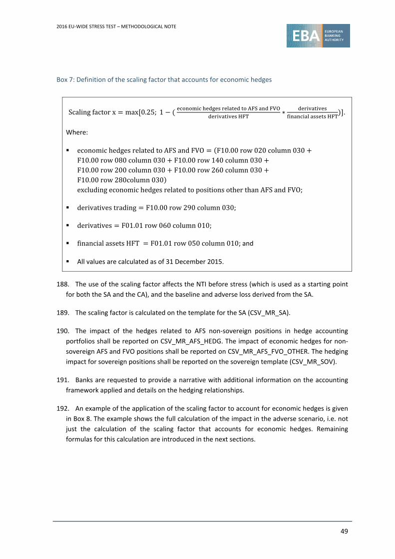
2016 EU‐WIDE STRESS TEST – METHODOLOGICAL NOTE
49
Box 7: Definition of the scaling factor that accounts for economic hedges
Scalingfactorx max 0.25; 1
∗
.
Where:
economichedgesrelatedtoAFSandFVO F10.00row020column030F10.00row080column030 F10.00row140column030F10.00row200column030 F10.00row260column030F10.00row280column030excludingeconomichedgesrelatedtopositionsotherthanAFSandFVO;
derivativestrading F10.00row290column030;
derivatives F01.01row060column010;
financialassetsHFT F01.01row050column010; and
All values are calculated as of 31 December 2015.
188. The use of the scaling factor affects the NTI before stress (which is used as a starting point
for both the SA and the CA), and the baseline and adverse loss derived from the SA.
189. The scaling factor is calculated on the template for the SA (CSV_MR_SA).
190. The impact of the hedges related to AFS non‐sovereign positions in hedge accounting
portfolios shall be reported on CSV_MR_AFS_HEDG. The impact of economic hedges for non‐
sovereign AFS and FVO positions shall be reported on CSV_MR_AFS_FVO_OTHER. The hedging
impact for sovereign positions shall be reported on the sovereign template (CSV_MR_SOV).
191. Banks are requested to provide a narrative with additional information on the accounting
framework applied and details on the hedging relationships.
192. An example of the application of the scaling factor to account for economic hedges is given
in Box 8. The example shows the full calculation of the impact in the adverse scenario, i.e. not
just the calculation of the scaling factor that accounts for economic hedges. Remaining
formulas for this calculation are introduced in the next sections.
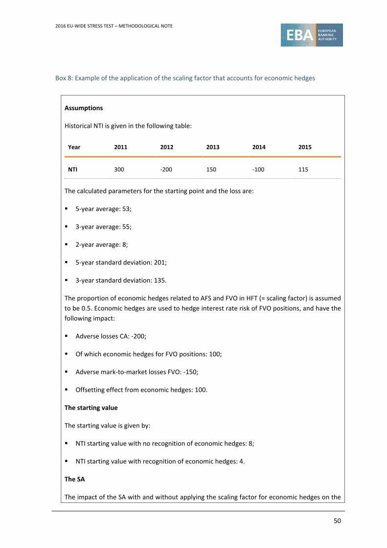
2016 EU‐WIDE STRESS TEST – METHODOLOGICAL NOTE
50
Box 8: Example of the application of the scaling factor that accounts for economic hedges
Assumptions
Historical NTI is given in the following table:
Year 2011 2012 2013 2014 2015
NTI 300 ‐200 150 ‐100 115
The calculated parameters for the starting point and the loss are:
5‐year average: 53;
3‐year average: 55;
2‐year average: 8;
5‐year standard deviation: 201;
3‐year standard deviation: 135.
The proportion of economic hedges related to AFS and FVO in HFT (= scaling factor) is assumed
to be 0.5. Economic hedges are used to hedge interest rate risk of FVO positions, and have the
following impact:
Adverse losses CA: ‐200;
Of which economic hedges for FVO positions: 100;
Adverse mark‐to‐market losses FVO: ‐150;
Offsetting effect from economic hedges: 100.
The starting value
The starting value is given by:
NTI starting value with no recognition of economic hedges: 8;
NTI starting value with recognition of economic hedges: 4.
The SA
The impact of the SA with and without applying the scaling factor for economic hedges on the
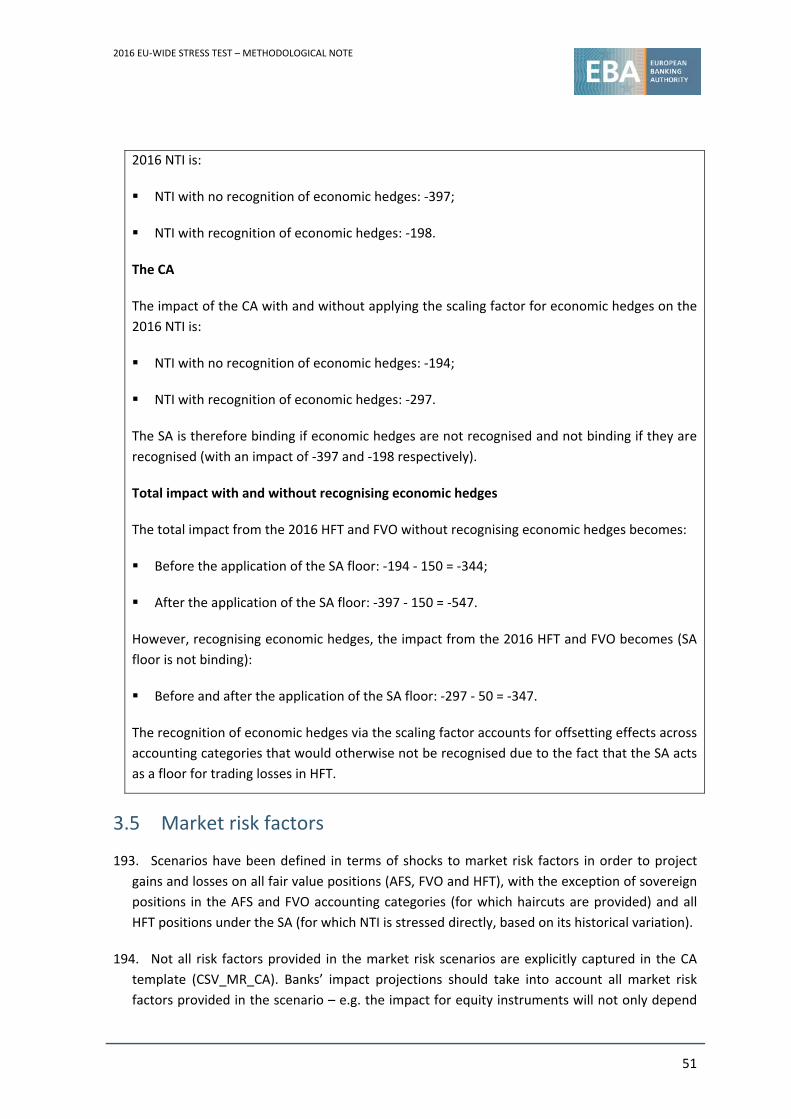
2016 EU‐WIDE STRESS TEST – METHODOLOGICAL NOTE
51
2016 NTI is:
NTI with no recognition of economic hedges: ‐397;
NTI with recognition of economic hedges: ‐198.
The CA
The impact of the CA with and without applying the scaling factor for economic hedges on the
2016 NTI is:
NTI with no recognition of economic hedges: ‐194;
NTI with recognition of economic hedges: ‐297.
The SA is therefore binding if economic hedges are not recognised and not binding if they are
recognised (with an impact of ‐397 and ‐198 respectively).
Total impact with and without recognising economic hedges
The total impact from the 2016 HFT and FVO without recognising economic hedges becomes:
Before the application of the SA floor: ‐194 ‐ 150 = ‐344;
After the application of the SA floor: ‐397 ‐ 150 = ‐547.
However, recognising economic hedges, the impact from the 2016 HFT and FVO becomes (SA
floor is not binding):
Before and after the application of the SA floor: ‐297 ‐ 50 = ‐347.
The recognition of economic hedges via the scaling factor accounts for offsetting effects across
accounting categories that would otherwise not be recognised due to the fact that the SA acts
as a floor for trading losses in HFT.
3.5 Market risk factors
193. Scenarios have been defined in terms of shocks to market risk factors in order to project
gains and losses on all fair value positions (AFS, FVO and HFT), with the exception of sovereign
positions in the AFS and FVO accounting categories (for which haircuts are provided) and all
HFT positions under the SA (for which NTI is stressed directly, based on its historical variation).
194. Not all risk factors provided in the market risk scenarios are explicitly captured in the CA
template (CSV_MR_CA). Banks’ impact projections should take into account all market risk
factors provided in the scenario – e.g. the impact for equity instruments will not only depend
2016 EU‐WIDE STRESS TEST – METHODOLOGICAL NOTE
52
on the shocks provided for equity indices, but also on the volatility assumptions in the
scenario.
195. The stressed market risk factors have been estimated for the adverse scenario by the ESRB
and the ECB. In addition, for the HFT accounting category, banks using the CA are provided
with two historical scenarios consistent with past stress events related to the global financial
crisis and the sovereign debt crisis.
196. As the risk factors provided may not necessarily capture all of banks’ market risk drivers in
the HFT portfolio, CA banks are required to report additional risk factors that are not included
in the scenario but have a material contribution – i.e. on a cumulative basis, the additional risk
factors show a relevant impact, and, along with the factors already considered, explain at least
95% of the actual VaR. In addition, banks need to report the calibration of these risk factors
and their impact in an accompanying document. This information will be relevant in the quality
assurance process in order to assess the degree of fitting between the additional stress factors
and the ones included in the scenarios.
197. Banks shall differentiate between two kinds of additional risk factors:
i. Risk factors that are part of aggregated risk factors in the given scenario – e.g.
swap rates or credit spreads as part of the aggregated risk factor provided for
Asia or different types of oil as part of the oil risk factor;
ii. Risk factors that are not included in the scenario in aggregate form – e.g. inflation
risk.
198. For the first type of risk factors defined in paragraph 197, banks shall, in general, not
extend the set of risk factors to additional more granular risk factors but shall apply the shocks
given in the scenario directly. However, banks should assess whether the resulting stress is
adequate for their portfolio. If this is not the case due to illiquid positions in a bank’s portfolio
or concentrations in more volatile positions, banks may also extend the scenario to more
granular risk factors. This approach may only increase the stress impact of the bank. Only the
impact for the second type of risk factors should be reported under additional risk factors.
199. In the case of interest rate and credit curves, the shocks for tenors that are not provided in
the market risk scenario should be computed by interpolation. For tenors that are shorter or
longer than the range of tenors available in the scenario, the the impact from shocks to the
shortest and the longest tenor available respectively should act as a floor.
200. CA banks should define their own approach to translate the scenarios to shocks to the
additional risk factors, and need to provide evidence to show that this approach is: i)
appropriate (i.e. methods and relationships relied upon should be valid); ii) comprehensive
(i.e. material market risks should not be left unstressed); iii) conservative (i.e. where it is
impossible to accurately reflect the impact of the stress scenario, banks should overestimate
2016 EU‐WIDE STRESS TEST – METHODOLOGICAL NOTE
53
rather than underestimate its impact); and iv) reviewed and governed (i.e. the process and
result have been checked and challenged by appropriate officers of the bank).
201. The treatment of additional risk factors, as well as the optional and additional information
required by competent authorities, is specified in Box 9. Data that is available in banks’ internal
systems and is sourced from standard market data providers can be used for the purpose of
calibrating shocks to the additional risk factors.
202. SA banks are not required to include additional risk factors in their projections.
Box 9: Treatment of additional risk factors
Banks should distinguish between additional risk factors that cannot be derived from the risk
factors provided by the EBA and the ones that can be directly derived from these risk factors, as
well as between the historical scenarios and the macroeconomic scenario.
In all the cases where supporting information is required, competent authorities will assess the
reliability of the shocks applied as part of the quality assurance process.
Approaches for the calibration of the shocks to additional risk factors directly derived from the
risk factors provided in the scenario
Most of the banks risk factors should be derived directly from the risk factors provided by the
scenario and reported in the associated rows in the CA template (CSV_MR_CA).
Where good quality data is available, one of the following approaches should be adopted:
Similar scenario: If good quality data from a historical scenario that is ‘similar’ to the
particular scenario is available, this should be used to calibrate the shift in the
additional risk factor. The corresponding evidence should be provided, including
reasons for deeming the alternative historical scenario to be similar (especially with
regard to the risk factor considered);
Calibrated statistical relationship between risk factors and additional risk factors: If
good quality data is available in sufficient quantity to support a statistical relationship
between the additional risk factor and one (or more) of the risk factors in the scenario
provided, this relationship should be used to calibrate the shock to the additional risk
factor, and the statistical evidence to support this relationship should be provided,
including evidence to indicate how this relationship holds up in stressed market
conditions.
Where good quality data is unavailable (e.g. for a newly issued corporate bond), such that the
variable itself is unobservable over the reference period and its relationship with other
variables cannot be statistically determined, theoretical reasons to support the calibration of
2016 EU‐WIDE STRESS TEST – METHODOLOGICAL NOTE
54
the risk factor shift should be provided. For example, there may be arbitrage reasons to
support the calibration. In particular, the value of certain illiquid and/or complex trading book
positions depends upon unobservable, or difficult to observe, parameters. Such parameters
(and the valuation methods in which they are used as inputs) should be adjusted to reflect the
severity of the market shock associated with the scenario. For example, if the severity of the
market shock might lead to circumstances that would require a re‐marking of the equity
correlation book, correlations, illiquid parameters, associated basis factors and the valuation
methodology should be adjusted accordingly.
Approaches for the calibration of the shocks to additional risk factors that cannot be derived
from the risk factors provided in the scenario
Some banks may have to add risk factors that are not correlated to the risk factors provided in
the scenario. The impact of these additional risk factors should be reported under the rows
for other risk factors in the CA template (CSV_MR_CA).
If good quality data is available in sufficient quantity to support a statistical relationship
between the risk factor and the macroeconomic variables for which projections are provided
in the macroeconomic scenario, this relationship should be used to calibrate the risk factor,
and the statistical evidence to support this relationship should be provided, including
evidence to indicate how this relationship holds up in stressed market conditions.
Where good quality data is unavailable such that the variable itself is unobservable over the
reference period or its relationship with other variables cannot be statistically determined,
theoretical reasons to support the calibration of the risk factor shift should be provided.
For historical scenarios
Banks have to project market risk losses under two different historical scenarios. The
historical periods that were considered when calibrating the scenarios are:
Historical scenario 1: Subprime crisis (June 2007 to October 2009)
Historical scenario 2: European sovereign debt crisis (April 2010 to September 2012)
Banks can estimate the shocks to be applied to the additional risk factors in different ways. In
any case, the estimated impact of the shock to a given risk factor under a specific scenario
cannot be lower than the impact obtained assuming a shock equal to the change in the risk
factor between the initial and the final dates indicated in the corresponding reference period
above. Where good quality data from the period referenced by the particular historical
scenario is available, banks shall use these data to calibrate the shift in the risk factor and the
corresponding evidence provided.
Where good quality data from the period referenced by the particular historical scenario is
unavailable (and only in this case), then one of the approaches for the calibration of the
2016 EU‐WIDE STRESS TEST – METHODOLOGICAL NOTE
55
shocks to additional risk factors presented above should be considered.
Macroeconomic adverse scenario
Macroeconomic adverse scenarios are hypothetical, and if no historical data specific for the
given scenario are available, then for the calibration of the shocks to additional risk factors,
the approaches listed above should be considered.
3.6 Impact on P&L and OCI – AFS and FVO positions
203. In the baseline scenario, no impact is assumed (i.e. the impact should be set to zero).
204. Prudential filters will be treated as prescribed in paragraph 25.
205. The impact on AFS and FVO positions shall be projected and reported by main asset classes
and, if relevant, maturities. In particular, banks need to report (depending on the portfolio):
The fair value or accounting value and notional of the positions;
The gain or losses broken down by risk factor;
The share of the impact that is hedged for hedge accounting portfolios (i.e. gains and
losses from hedged risk) or economic hedges and gains and losses from hedging for
other portfolios.
206. The total impact shall then be separately reported for the following items:
The impact on OCI from revaluation effects of non‐hedged risk factors on hedged item
– i.e. the impact on OCI after hedging;
Gains and losses from hedging ineffectiveness (attributable to P&L);
Gains and losses on FVO positions (attributable to P&L);
Gains and losses from economic hedges (attributable to P&L).
207. Resulting gains and losses on FVO positions shall be reported separately in the P&L
template (CSV_P&L) for sovereign and non‐sovereign positions.
208. Resulting gains and losses on AFS positions due to market price movements directly impact
the OCI, and shall be separately reported in the capital template (CSV_CAP) for sovereign and
non‐sovereign positions.
2016 EU‐WIDE STRESS TEST – METHODOLOGICAL NOTE
56
3.6.1 Non‐sovereign
209. Banks are requested to conduct full revaluations of their positions for the adverse
macroeconomic scenario (see section 3.5) and recognise the impact on P&L or OCI, in line with
accounting standards.
210. In line with paragraph 176, gains and losses on AFS and FVO non‐sovereign positions shall
be fully recognised in the first year of the stress test.
211. For the purpose of the stress test, banks shall not take into account possible valuation
adjustments on debt securities and gains resulting from credit spread widening of own
liabilities under any circumstances. Hence, following a deterioration of own creditworthiness,
the bank is not allowed to book a gain on those debt securities (or any other fair valued
liabilities) that represent a net liability to the bank.
212. The relevant positions and projections (including the impact of hedging) shall be reported
on CSV_MR_AFS_HEDG and CSV_MR_AFS_FVO_OTHER, depending on whether an AFS
position is within hedge accounting portfolios or not.
213. If an AFS position is within a hedge accounting portfolio but also hedged with an economic
hedge and the bank recognises economic hedges, the position shall be reported on
CSV_MR_AFS_HEDG but the economic hedge on CSV_AFS_FVO_OTHER.
3.6.2 Sovereign
214. Banks are required to report and stress both direct sovereign exposure by country and
residual maturity and related hedges for the adverse scenario. Exposures are reported as book
value and gross of hedging. The hedging effect is reported separately.
215. Sovereign positions in AFS and FVO are subject to the market risk parameters (mark‐to‐
market) and haircuts corresponding to the year 2016 as provided by the ESRB and the ECB. The
haircuts separate the (general) interest rate impact (swap rate change) and the credit spread
impact (sovereign spread over swap) for a specific sovereign and residual maturity. The shock
is allocated to the first year of the scenario (i.e. 2016). No shock or recovery is foreseen for the
subsequent years of the scenario. Haircuts are applied to direct exposures only (see definition
in section 3.3.1). Whenever available banks are required to use the haircuts provided. For
countries or regions for which no haircuts are provided banks should apply the
macroeconomic adverse market risk scenario.
216. In line with section 3.4, the stress for the corresponding hedging positions should be based
on the application of the same risk factor shocks (i.e. interest rates and credit spreads only) as
for the related hedged sovereign positions. It is assumed that the banks will not be able to
benefit from any potential misalignment of the shocks on hedged sovereign positions (i.e.
haircuts) and the market risk shocks on hedging instruments. The offsetting effect from
hedging instruments on sovereign positions in AFS and FVO must be proportionate to the
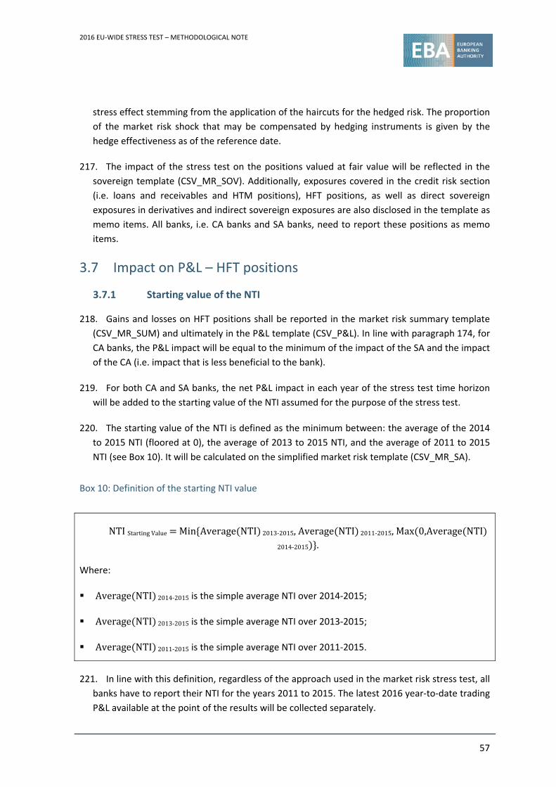
2016 EU‐WIDE STRESS TEST – METHODOLOGICAL NOTE
57
stress effect stemming from the application of the haircuts for the hedged risk. The proportion
of the market risk shock that may be compensated by hedging instruments is given by the
hedge effectiveness as of the reference date.
217. The impact of the stress test on the positions valued at fair value will be reflected in the
sovereign template (CSV_MR_SOV). Additionally, exposures covered in the credit risk section
(i.e. loans and receivables and HTM positions), HFT positions, as well as direct sovereign
exposures in derivatives and indirect sovereign exposures are also disclosed in the template as
memo items. All banks, i.e. CA banks and SA banks, need to report these positions as memo
items.
3.7 Impact on P&L – HFT positions
3.7.1 Starting value of the NTI
218. Gains and losses on HFT positions shall be reported in the market risk summary template
(CSV_MR_SUM) and ultimately in the P&L template (CSV_P&L). In line with paragraph 174, for
CA banks, the P&L impact will be equal to the minimum of the impact of the SA and the impact
of the CA (i.e. impact that is less beneficial to the bank).
219. For both CA and SA banks, the net P&L impact in each year of the stress test time horizon
will be added to the starting value of the NTI assumed for the purpose of the stress test.
220. The starting value of the NTI is defined as the minimum between: the average of the 2014
to 2015 NTI (floored at 0), the average of 2013 to 2015 NTI, and the average of 2011 to 2015
NTI (see Box 10). It will be calculated on the simplified market risk template (CSV_MR_SA).
Box 10: Definition of the starting NTI value
NTIStartingValue Min Average NTI 2013‐2015, Average NTI 2011‐2015,Max 0,Average NTI
2014‐2015 .
Where:
Average NTI 2014‐2015 is the simple average NTI over 2014‐2015;
Average NTI 2013‐2015 is the simple average NTI over 2013‐2015;
Average NTI 2011‐2015 is the simple average NTI over 2011‐2015.
221. In line with this definition, regardless of the approach used in the market risk stress test, all
banks have to report their NTI for the years 2011 to 2015. The latest 2016 year‐to‐date trading
P&L available at the point of the results will be collected separately.
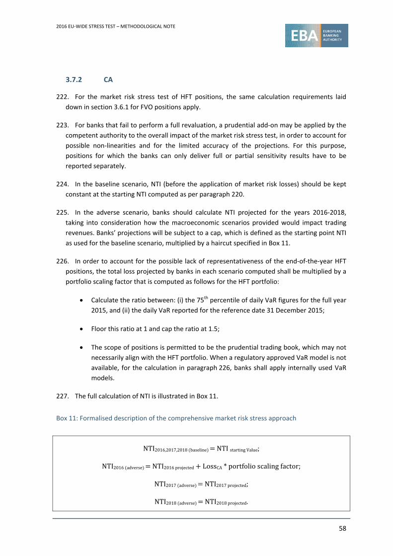
2016 EU‐WIDE STRESS TEST – METHODOLOGICAL NOTE
58
3.7.2 CA
222. For the market risk stress test of HFT positions, the same calculation requirements laid
down in section 3.6.1 for FVO positions apply.
223. For banks that fail to perform a full revaluation, a prudential add‐on may be applied by the
competent authority to the overall impact of the market risk stress test, in order to account for
possible non‐linearities and for the limited accuracy of the projections. For this purpose,
positions for which the banks can only deliver full or partial sensitivity results have to be
reported separately.
224. In the baseline scenario, NTI (before the application of market risk losses) should be kept
constant at the starting NTI computed as per paragraph 220.
225. In the adverse scenario, banks should calculate NTI projected for the years 2016‐2018,
taking into consideration how the macroeconomic scenarios provided would impact trading
revenues. Banks’ projections will be subject to a cap, which is defined as the starting point NTI
as used for the baseline scenario, multiplied by a haircut specified in Box 11.
226. In order to account for the possible lack of representativeness of the end‐of‐the‐year HFT
positions, the total loss projected by banks in each scenario computed shall be multiplied by a
portfolio scaling factor that is computed as follows for the HFT portfolio:
Calculate the ratio between: (i) the 75th percentile of daily VaR figures for the full year
2015, and (ii) the daily VaR reported for the reference date 31 December 2015;
Floor this ratio at 1 and cap the ratio at 1.5;
The scope of positions is permitted to be the prudential trading book, which may not
necessarily align with the HFT portfolio. When a regulatory approved VaR model is not
available, for the calculation in paragraph 226, banks shall apply internally used VaR
models.
227. The full calculation of NTI is illustrated in Box 11.
Box 11: Formalised description of the comprehensive market risk stress approach
NTI2016,2017,2018 baseline NTIstartingValue;
NTI2016 adverse NTI2016projected LossCA*portfolioscalingfactor;
NTI2017 adverse NTI2017projected;
NTI2018 adverse NTI2018projected.
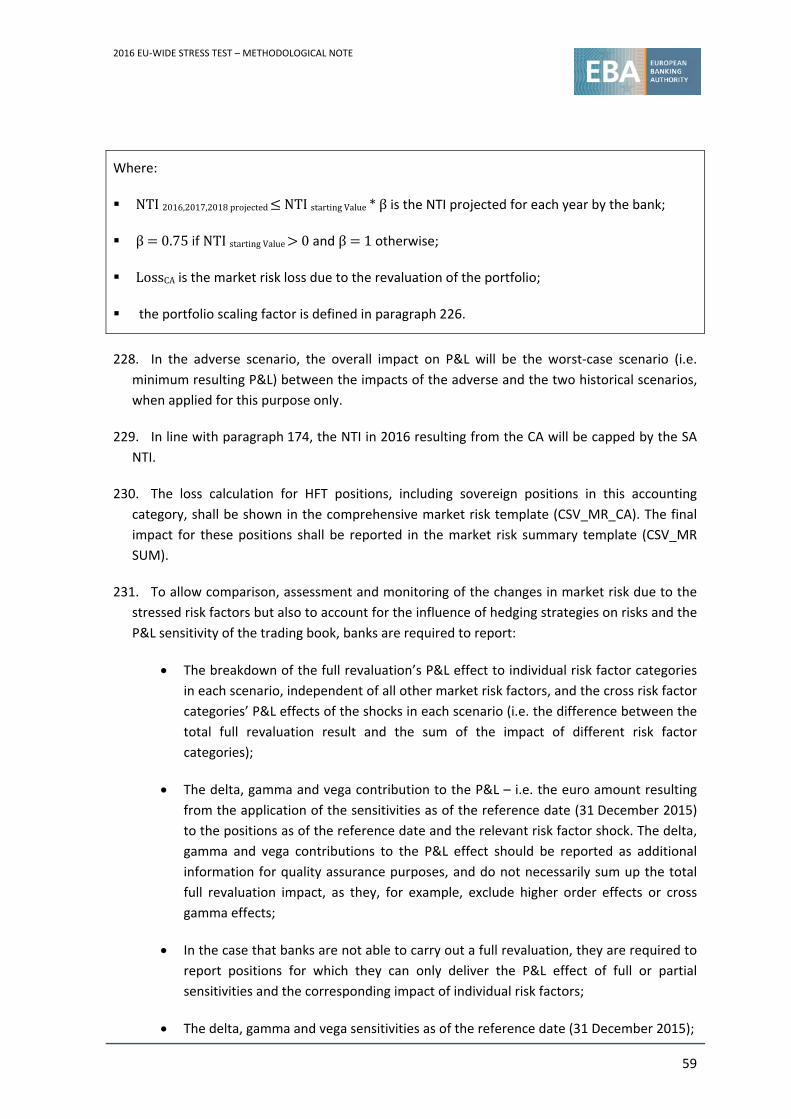
2016 EU‐WIDE STRESS TEST – METHODOLOGICAL NOTE
59
Where:
NTI2016,2017,2018projected NTIstartingValue*β is the NTI projected for each year by the bank;
β 0.75 if NTIstartingValue 0 and β 1 otherwise;
LossCA is the market risk loss due to the revaluation of the portfolio;
the portfolio scaling factor is defined in paragraph 226.
228. In the adverse scenario, the overall impact on P&L will be the worst‐case scenario (i.e.
minimum resulting P&L) between the impacts of the adverse and the two historical scenarios,
when applied for this purpose only.
229. In line with paragraph 174, the NTI in 2016 resulting from the CA will be capped by the SA
NTI.
230. The loss calculation for HFT positions, including sovereign positions in this accounting
category, shall be shown in the comprehensive market risk template (CSV_MR_CA). The final
impact for these positions shall be reported in the market risk summary template (CSV_MR
SUM).
231. To allow comparison, assessment and monitoring of the changes in market risk due to the
stressed risk factors but also to account for the influence of hedging strategies on risks and the
P&L sensitivity of the trading book, banks are required to report:
The breakdown of the full revaluation’s P&L effect to individual risk factor categories
in each scenario, independent of all other market risk factors, and the cross risk factor
categories’ P&L effects of the shocks in each scenario (i.e. the difference between the
total full revaluation result and the sum of the impact of different risk factor
categories);
The delta, gamma and vega contribution to the P&L – i.e. the euro amount resulting
from the application of the sensitivities as of the reference date (31 December 2015)
to the positions as of the reference date and the relevant risk factor shock. The delta,
gamma and vega contributions to the P&L effect should be reported as additional
information for quality assurance purposes, and do not necessarily sum up the total
full revaluation impact, as they, for example, exclude higher order effects or cross
gamma effects;
In the case that banks are not able to carry out a full revaluation, they are required to
report positions for which they can only deliver the P&L effect of full or partial
sensitivities and the corresponding impact of individual risk factors;
The delta, gamma and vega sensitivities as of the reference date (31 December 2015);
2016 EU‐WIDE STRESS TEST – METHODOLOGICAL NOTE
60
The stand‐alone VaR per risk factor category for HFT positions. If the bank does have
an approved VaR model in use for a factor category internally used, the VaR models
shall be applied;
The fair value by risk factor category. If positions are subject to several risk factor
categories, they should be allocated in full to all relevant risk factor categories. The
total fair value reported as of 31 December 2015 can therefore deviate from the sum
of the fair value across risk factor categories.
232. CA banks shall also compute the market liquidity shock due to an exogenous widening in
the bid‐ask spread for the whole HFT portfolio.
233. The impact of different risk factors should be reported without basis risk. Banks should
report the impact of all their basis risks separately, and use their own methodology to stress
basis risk. Key basis risks are expected to cover (inter alia) interest rates, credit spreads and
commodity prices. In all cases, banks should assume relative changes in the bases (compared
to the values observed as of 31 December 2015) that are consistent with the scenario. For
each basis risk factor, a positive impact from the change in the basis shall be set to zero,
allowing only for a negative impact of the full revaluation. Competent authorities can ask
banks to provide more granular information on the impact of basis risk.
234. In general the market shocks are intended to be applied and reported not at product level
but rather by relevant risk factors. For instance for a bond the key risk factors to be considered
are interest rate and credit risk. Exceptions to this general rule are represented for example by
funds, RMBS and CMBS for which the scenarios do include the relative change in the fair value
respectively the yield of the products and for which there is no need to disentangle the effects
in underlying shocks. In case of asset classes similar to the ones for which fair value changes
are given, banks shall apply the same approach and shocks. For example for covered bonds the
relative shocks for senior RMBS and CMBS shall be applied. For structured products with
embedded derivatives (e.g. optionalities) the bank is expected to disentangle the financial
instrument in its main components (e.g. plain vanilla bond and options) before the application
of the market risk factor shocks.
235. The impact of the shock on correlation trading portfolios shall be reported by relevant risk
factors together with other positions on the CA market risk template (CSV_MR_CA). CA banks
holding a correlation trading portfolio in excess of 1% of total REA are deemed to hold a
significant correlation trading portfolio. Competent authorities can ask these banks to provide
additional information on the impact of these portfolios.
236. When reporting results for the HFT positions, multivariate effects, as well as scenario
correlation assumptions deriving from the application of the market risk parameter shocks,
shall be taken into account and cumulatively shown in the template (CSV_MR_CA) for each
major class of risk factors (separately from the one‐factor P&L effects). For the macroeconomic
scenarios and each of the two historical scenarios, the total P&L effect stemming from the
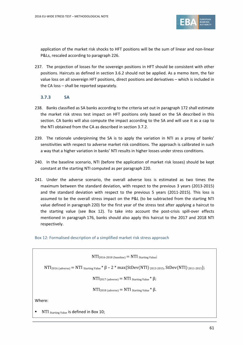
2016 EU‐WIDE STRESS TEST – METHODOLOGICAL NOTE
61
application of the market risk shocks to HFT positions will be the sum of linear and non‐linear
P&Ls, rescaled according to paragraph 226.
237. The projection of losses for the sovereign positions in HFT should be consistent with other
positions. Haircuts as defined in section 3.6.2 should not be applied. As a memo item, the fair
value loss on all sovereign HFT positions, direct positions and derivatives – which is included in
the CA loss – shall be reported separately.
3.7.3 SA
238. Banks classified as SA banks according to the criteria set out in paragraph 172 shall estimate
the market risk stress test impact on HFT positions only based on the SA described in this
section. CA banks will also compute the impact according to the SA and will use it as a cap to
the NTI obtained from the CA as described in section 3.7.2.
239. The rationale underpinning the SA is to apply the variation in NTI as a proxy of banks’
sensitivities with respect to adverse market risk conditions. The approach is calibrated in such
a way that a higher variation in banks’ NTI results in higher losses under stress conditions.
240. In the baseline scenario, NTI (before the application of market risk losses) should be kept
constant at the starting NTI computed as per paragraph 220.
241. Under the adverse scenario, the overall adverse loss is estimated as two times the
maximum between the standard deviation, with respect to the previous 3 years (2013‐2015)
and the standard deviation with respect to the previous 5 years (2011‐2015). This loss is
assumed to be the overall stress impact on the P&L (to be subtracted from the starting NTI
value defined in paragraph 220) for the first year of the stress test after applying a haircut to
the starting value (see Box 12). To take into account the post‐crisis spill‐over effects
mentioned in paragraph 176, banks should also apply this haircut to the 2017 and 2018 NTI
respectively.
Box 12: Formalised description of a simplified market risk stress approach
NTI2016‐2018 baseline NTIStartingValue;
NTI2016 adverse NTIStartingValue*β–2*max StDev NTI 2013‐2015,StDev NTI 2011‐2015 ;
NTI2017 adverse NTIStartingValue*β;
NTI2018 adverse NTIStartingValue*β.
Where:
NTIStartingValue is defined in Box 10;
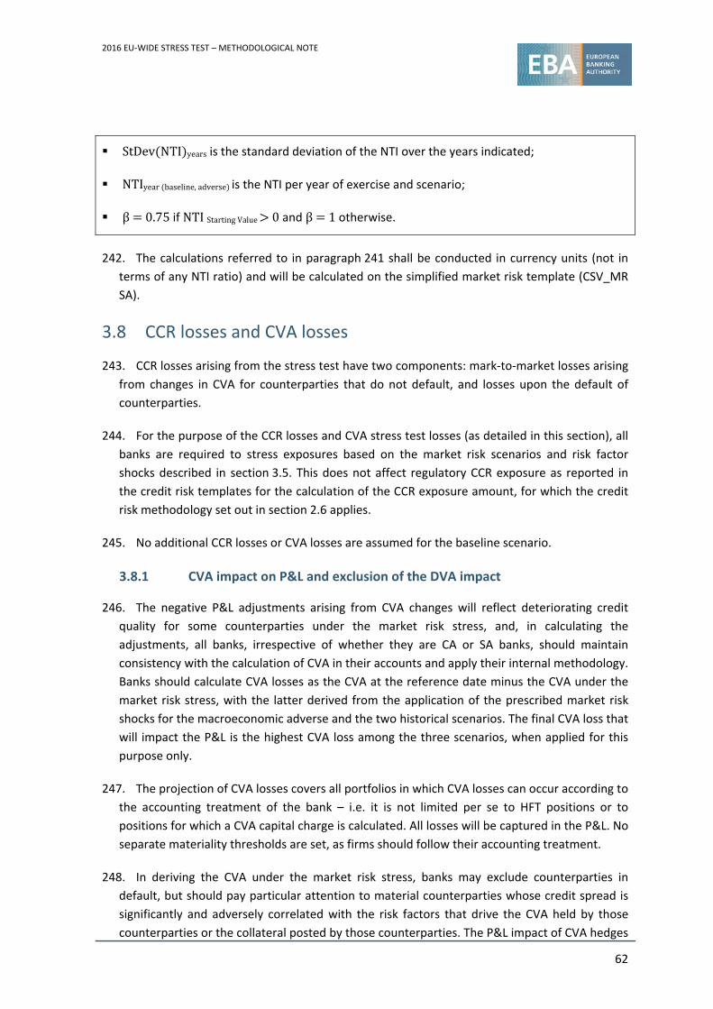
2016 EU‐WIDE STRESS TEST – METHODOLOGICAL NOTE
62
StDev NTI years is the standard deviation of the NTI over the years indicated;
NTIyear baseline,adverse is the NTI per year of exercise and scenario;
β 0.75 if NTIStartingValue 0 and β 1 otherwise.
242. The calculations referred to in paragraph 241 shall be conducted in currency units (not in
terms of any NTI ratio) and will be calculated on the simplified market risk template (CSV_MR
SA).
3.8 CCR losses and CVA losses
243. CCR losses arising from the stress test have two components: mark‐to‐market losses arising
from changes in CVA for counterparties that do not default, and losses upon the default of
counterparties.
244. For the purpose of the CCR losses and CVA stress test losses (as detailed in this section), all
banks are required to stress exposures based on the market risk scenarios and risk factor
shocks described in section 3.5. This does not affect regulatory CCR exposure as reported in
the credit risk templates for the calculation of the CCR exposure amount, for which the credit
risk methodology set out in section 2.6 applies.
245. No additional CCR losses or CVA losses are assumed for the baseline scenario.
3.8.1 CVA impact on P&L and exclusion of the DVA impact
246. The negative P&L adjustments arising from CVA changes will reflect deteriorating credit
quality for some counterparties under the market risk stress, and, in calculating the
adjustments, all banks, irrespective of whether they are CA or SA banks, should maintain
consistency with the calculation of CVA in their accounts and apply their internal methodology.
Banks should calculate CVA losses as the CVA at the reference date minus the CVA under the
market risk stress, with the latter derived from the application of the prescribed market risk
shocks for the macroeconomic adverse and the two historical scenarios. The final CVA loss that
will impact the P&L is the highest CVA loss among the three scenarios, when applied for this
purpose only.
247. The projection of CVA losses covers all portfolios in which CVA losses can occur according to
the accounting treatment of the bank – i.e. it is not limited per se to HFT positions or to
positions for which a CVA capital charge is calculated. All losses will be captured in the P&L. No
separate materiality thresholds are set, as firms should follow their accounting treatment.
248. In deriving the CVA under the market risk stress, banks may exclude counterparties in
default, but should pay particular attention to material counterparties whose credit spread is
significantly and adversely correlated with the risk factors that drive the CVA held by those
counterparties or the collateral posted by those counterparties. The P&L impact of CVA hedges
2016 EU‐WIDE STRESS TEST – METHODOLOGICAL NOTE
63
in place at the reference date should be recognised, but no adjustment to those hedges should
be assumed.
249. For the purposes of the stress test, the banks shall not take into account possible DVA.
Hence, following a deterioration of own creditworthiness, the bank is not allowed to book a
P&L profit on those derivatives (or any other fair valued liability) that present a net liability to
the bank.
250. Banks are not allowed to offset the projected CVA fair value impact by any existing
reserves.
251. The resulting CVA impact shall be reported using the CVA template (CSV_MR_CVA).
3.8.2 Counterparty defaults
252. In addition to the P&L associated with changes in CVAs, counterparty credit losses may
arise if counterparties actually default in the stress. This is calculated in the CCR template
(CSV_MR_CCR). To gauge the possible impact of this source of P&L, competent authorities will
require banks to calculate and report CCR exposure as at the reference date, stressed
exposure, and appropriate stressed LGD for their top 10 largest counterparties, as described
below.
253. In considering counterparty defaults in conjunction with market risk stresses, market risk
factor shocks should be applied to the exposure, whether uncollateralised or collateralised. In
the case of collateralised exposures, banks should also stress the collateral in line with the
market risk shocks, assuming (in line with the general assumption of no portfolio rebalancing)
that no additional collateral is provided beyond what is currently held. Exposures should be
stressed based on the scenarios as defined in section 3.5.
254. To identify their top 10 largest counterparties, banks should rank their counterparties in all
accounting portfolios subject to CCR (i.e. including HFT, AFS, FVO and HTM) by stressed current
exposure after netting (if contractually permitted) for the macroeconomic adverse and the two
historical scenarios. Collateralised and uncollateralised exposure should be included in this
ranking. Exposure shall be reported net of stressed collateral. No collateral that is to be called
beyond what is held at the reference date may be assumed.
255. For each of the three scenarios, banks are required to assume the default of the two most
vulnerable counterparties within their top 10 largest counterparties – i.e. depending on the
impact of the scenario, two different counterparties can be assumed to default.
256. Central governments, central banks, CCPs and other market infrastructures, counterparties
explicitly guaranteed by the central government and intra‐group exposures should not be
included in the set of counterparties and names used to identify the largest exposure.
2016 EU‐WIDE STRESS TEST – METHODOLOGICAL NOTE
64
257. The selection of the two most vulnerable counterparties involves judgement on the part of
the bank of the creditworthiness of these counterparties, in the light of the size of the
exposures. In making this judgement, banks should consider both the current creditworthiness
of these counterparties and how that creditworthiness might deteriorate under the scenario in
question. The judgement of the bank should not be based on a simple application of measures,
such as banking book PDs and external credit ratings, but should also take into account
idiosyncratic credit factors that would not necessarily be captured in such measures, again
with particular reference to the scenario in question. Banks should pay particular attention to
exposures to shadow banks and exposures to counterparties exposed to commodity risk.
258. The overall CCR loss will be calculated as the default exposure of the counterparty
identified in paragraph 257 multiplied by the appropriate stressed LGD and minus the
accounting CVA impact on P&L (before the application of the market price stress). Here, the
appropriate stressed LGD should be consistent with the banking book risk parameters
estimates carried out by the bank. This loss will be added to the total losses resulting from the
market risk scenario.
259. The final loss stemming from the default of the two most vulnerable counterparties that
will impact the P&L is the highest CCR loss among the three scenarios, when applied for this
purpose only.
260. The default of the two most vulnerable counterparties covers the effect that the whole CCR
exposure assigned to this counterparty has on the P&L in case the counterparty defaults. In
addition to the CCR exposure, banks are asked to calculate losses from the jump‐to‐default of
the direct credit exposure to this counterparty in the HFT, AFS and FVO portfolios. Here jump‐
to‐default is the net profit or loss resulting from an issuer’s instantaneous default. Indirect
exposures to the issuer (i.e. CDS) should be included, as this corresponds to the default of the
reference entity.
261. The algorithm for identifying and defaulting CCR exposures is summarised in Box 13.
262. The resulting losses will be captured as impairments in the P&L. The projection of
counterparty defaults should be carried out independently from the projection of credit risk
losses as defined in section 2.4 – i.e. no adjustments should be made for credit risk exposure
or credit risk parameters for the projection of credit risk losses as defined in section 2.4, based
on assumed counterparty defaults.
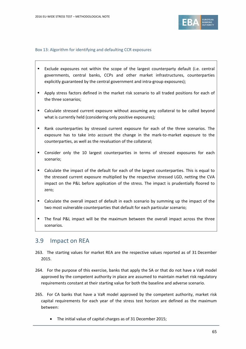
2016 EU‐WIDE STRESS TEST – METHODOLOGICAL NOTE
65
Box 13: Algorithm for identifying and defaulting CCR exposures
Exclude exposures not within the scope of the largest counterparty default (i.e. central
governments, central banks, CCPs and other market infrastructures, counterparties
explicitly guaranteed by the central government and intra‐group exposures);
Apply stress factors defined in the market risk scenario to all traded positions for each of
the three scenarios;
Calculate stressed current exposure without assuming any collateral to be called beyond
what is currently held (considering only positive exposures);
Rank counterparties by stressed current exposure for each of the three scenarios. The
exposure has to take into account the change in the mark‐to‐market exposure to the
counterparties, as well as the revaluation of the collateral;
Consider only the 10 largest counterparties in terms of stressed exposures for each
scenario;
Calculate the impact of the default for each of the largest counterparties. This is equal to
the stressed current exposure multiplied by the respective stressed LGD, netting the CVA
impact on the P&L before application of the stress. The impact is prudentially floored to
zero;
Calculate the overall impact of default in each scenario by summing up the impact of the
two most vulnerable counterparties that default for each particular scenario;
The final P&L impact will be the maximum between the overall impact across the three
scenarios.
3.9 Impact on REA
263. The starting values for market REA are the respective values reported as of 31 December
2015.
264. For the purpose of this exercise, banks that apply the SA or that do not have a VaR model
approved by the competent authority in place are assumed to maintain market risk regulatory
requirements constant at their starting value for both the baseline and adverse scenario.
265. For CA banks that have a VaR model approved by the competent authority, market risk
capital requirements for each year of the stress test horizon are defined as the maximum
between:
The initial value of capital charges as of 31 December 2015;
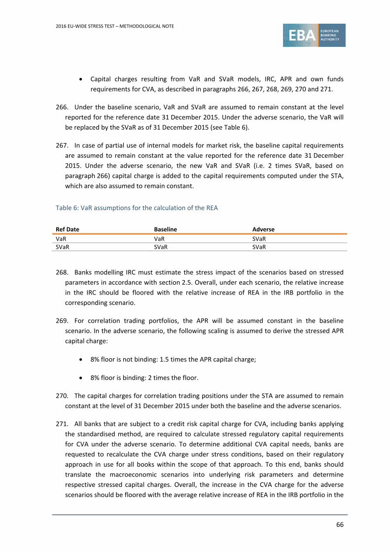
2016 EU‐WIDE STRESS TEST – METHODOLOGICAL NOTE
66
Capital charges resulting from VaR and SVaR models, IRC, APR and own funds
requirements for CVA, as described in paragraphs 266, 267, 268, 269, 270 and 271.
266. Under the baseline scenario, VaR and SVaR are assumed to remain constant at the level
reported for the reference date 31 December 2015. Under the adverse scenario, the VaR will
be replaced by the SVaR as of 31 December 2015 (see Table 6).
267. In case of partial use of internal models for market risk, the baseline capital requirements
are assumed to remain constant at the value reported for the reference date 31 December
2015. Under the adverse scenario, the new VaR and SVaR (i.e. 2 times SVaR, based on
paragraph 266) capital charge is added to the capital requirements computed under the STA,
which are also assumed to remain constant.
Table 6: VaR assumptions for the calculation of the REA
Ref Date Baseline Adverse
VaR VaR SVaRSVaR SVaR SVaR
268. Banks modelling IRC must estimate the stress impact of the scenarios based on stressed
parameters in accordance with section 2.5. Overall, under each scenario, the relative increase
in the IRC should be floored with the relative increase of REA in the IRB portfolio in the
corresponding scenario.
269. For correlation trading portfolios, the APR will be assumed constant in the baseline
scenario. In the adverse scenario, the following scaling is assumed to derive the stressed APR
capital charge:
8% floor is not binding: 1.5 times the APR capital charge;
8% floor is binding: 2 times the floor.
270. The capital charges for correlation trading positions under the STA are assumed to remain
constant at the level of 31 December 2015 under both the baseline and the adverse scenarios.
271. All banks that are subject to a credit risk capital charge for CVA, including banks applying
the standardised method, are required to calculate stressed regulatory capital requirements
for CVA under the adverse scenario. To determine additional CVA capital needs, banks are
requested to recalculate the CVA charge under stress conditions, based on their regulatory
approach in use for all books within the scope of that approach. To this end, banks should
translate the macroeconomic scenarios into underlying risk parameters and determine
respective stressed capital charges. Overall, the increase in the CVA charge for the adverse
scenarios should be floored with the average relative increase of REA in the IRB portfolio in the

2016 EU‐WIDE STRESS TEST – METHODOLOGICAL NOTE
67
corresponding scenario. To be consistent with the approach for the CCR exposure amount, the
regulatory exposure used for the calculation of the stressed CVA REA shall be kept constant.
272. The impact on REA shall be reported using the market REA templates, depending on the
whether the SA or the CA is applied (CSV_REA_MR_CVA_SA or CSV_REA_MR_CVA_CA).
273. REA for the CCR capital requirements are calculated using the approach described in
section 2.6.
274. Finally, REA for securitisation positions are expected to change in accordance with the
securitisation methodology described in section 2.7 as part of the credit risk methodology.
2016 EU‐WIDE STRESS TEST – METHODOLOGICAL NOTE
68
4. NII
4.1 Overview
275. Banks may use their own methodology and their existing ALM systems and EaR models to
project their NII, relying on their assumptions regarding the pace of the repricing of their
portfolio, together with their projections for risk‐free reference rates and margins both under
the baseline and the adverse scenarios. The split between reference rate and margin
components of banks’ assets and liabilities is introduced to distinguish two risks affecting
banks’ NII under stress:
The risk related to a sudden change in the general ‘risk‐free’ yield curves. This risk is
aimed to be captured via the changes in the reference rate components of banks’
repriced assets and liabilities and off‐balance‐sheet short‐term and long‐term
positions;
The risk related to a sudden change in the ‘premium’ that the market requires or the
bank sets for different types of instruments and counterparties, reflecting the impact
on credit and other market risks (e.g. liquidity).
276. Banks’ projections are subject to the constraints summarised in Box 14.
Box 14: Summary of the constraints on banks’ projections of NII
Assumptions underlying the scenarios cannot lead (at group level) to an increase of the
bank’s NII, compared with the 2015 value, neither under the baseline scenario nor the
adverse scenario (paragraph 308).
Banks’ interest expenses cannot decline at group level under the adverse scenario,
compared with the 2015 value (paragraph 309).
Under the adverse scenario, income on defaulted assets should not be recognised, with the
exception of income stemming from discount unwinding. Income from discount unwinding is
capped by the 2015 value, and is subject to a constraint depending on the changes in
provisions and defaulted exposure (paragraph 310).
Under the baseline scenario, banks are required at a minimum to reflect a proportion of the
changes in the sovereign bond spread of the country of exposure in the margin component
of the EIR of their repriced liabilities (paragraph 327).
Under the adverse scenario, the margin paid on interest‐bearing liabilities cannot increase
2016 EU‐WIDE STRESS TEST – METHODOLOGICAL NOTE
69
less than the higher between a proportion of the increase in the sovereign spreads of the
country of exposure and the same proportion applied to the increase of an idiosyncratic
component, derived from the impact on banks’ wholesale funding rate of a rating
downgrade (paragraph 327).
Banks are required to cap the margin component of the EIR on their repriced assets by a
proportion of the increase in the sovereign spreads of the country of exposure
(paragraph 330).
Although no methodological constraints are imposed on the reference rate of newly
originated instruments, it is expected that the change in the reference rate of these
instruments is consistent with the macro‐financial scenarios for risk‐free yield curves
(paragraph 320).
4.2 Scope
277. All interest‐earning or interest‐paying positions across all accounting categories, including
not only instruments subject to amortised cost measurement but also those subject to fair
value measurement (such as HFT positions, AFS positions, FVO positions, and hedge
accounting instruments), are in the scope of this section.
278. Banks that, in the course of their periodic financial reporting, present the interest income
on assets in HFT, AFS, and FVO as a part of NTI, should report this income as a part of NII and
remove it from the recurring NTI in line with the provisions of paragraph 161 of this note. Only
NII for these positions is within the scope of the NII methodology; the fair value impact on
these positions of the stress test scenarios is captured within the market risk methodology,
and the impact on the economic value of equity, as required for Pillar II analysis, is not needed.
The fair value impact on derivatives not recognised for hedge accounting should continue to
be recognised in the market risk templates, in addition to this NII impact.
279. Fees and commissions that are recognised as NII in the accounting framework are also
within the scope of this section. The fees and commissions that can be directly linked to loans
should be stressed through the loan’s EIR. All other fee and commission income is out of the
scope of the NII methodology.
280. Banks are required to provide information on both their fixed and floating rate portfolios.
281. Banks are requested to split their derivatives positions between ‘derivatives used for hedge
accounting’ and ‘derivatives not used for hedge accounting’.
282. The definition of ‘hedge accounting instruments’ is in line with paragraph 154, i.e. the
FINREP definition. Other derivative instruments should be reported under ‘derivatives not
used for hedge accounting’ throughout the stress period. Banks are requested to provide a
2016 EU‐WIDE STRESS TEST – METHODOLOGICAL NOTE
70
narrative with additional information on the accounting framework applied and details on the
hedging relationships.
4.3 High‐level assumptions and definitions
4.3.1 Definitions
283. Banks are required to apply consistent definitions for the following items.
284. Reference interest rate (Ref Rate) is defined as the general underlying ‘risk‐free’7 rate
relevant for the given instrument, as used by banks in the management of their interest rate
risk in the banking book.8 That rate should not include instrument‐specific or entity‐specific
credit risk spreads or liquidity risk spreads. Examples of acceptable rates are swap rates, or, for
reference rate tenors below 1 year, the applicable interbank rate (e.g. EURIBOR, LIBOR). For
fixed‐rate instruments, banks should use the same reference rate curve for all instruments
denominated in a given currency, originated at the same time, and the reference rate tenor
should align with the original maturity of the instrument. For floating rate instruments,
instruments may be contractually linked to a particular reference rate, in which case this rate
should be used as the reference rate instead.
285. Margin is defined as the ‘premium’ charged/paid by banks over the instrument’s/
portfolio’s reference rate, and is equal to the spread between the actual rate of the instrument
and the reference rate.
286. Effective Interest Rate (EIR) for a given instrument, time interval and component (margin
or reference rate) is the rate that equals the ratio of interest income/expenses to the average
volume.
287. Maturity date is defined as the contractual date on which the Margin or the Ref Rate
component of the asset/liability is repriced:
For fixed‐rate instruments it is assumed that the maturity dates of the Ref Rate and
the Margin are the same, and equal to the contractual maturity of the instrument;
For floating rate instruments it is assumed that the Margin is repriced at the
contractual maturity of the instrument, while the Ref Rate component is repriced
whenever the index rate of the floating rate instrument resets.9 Therefore, the
maturity dates for the Ref Rate and the Margin of floating rate instruments will, in
many cases, be different. It is generally expected that the Ref Rate component resets
prior to the Margin in most of the cases.
7 The free‐yield curve shall be the one provided in the scenario, when available. 8 See the EBA Guidelines on the management of interest rate risk arising from non‐trading activities (EBA/GL/2015/08). 9 In this context, as mentioned above, for floating rate products, the index rate of the instrument should be used as the reference interest rate.
2016 EU‐WIDE STRESS TEST – METHODOLOGICAL NOTE
71
288. Original maturity is defined as the total time between the asset/liability’s time of
origination and the maturity date.
289. Average point of maturing is defined as the average fraction of a year at which the
maturing positions mature. For each relevant portfolio, the average point of maturing should
be computed as an average across the maturing positions in the years 2016‐2018. The
maturing positions to be considered in this context are those contained in the maturity
schedule at the cut‐off date10.
290. Existing position (Exist) refers to the volume, which is not repriced within the time interval
of interest.
291. Maturing position (Vol Mat) refers to the average volume of instruments maturing within
the time interval (i.e. exiting the stock of existing positions of the previous year). The average
volume is computed as the product of the notional amount of maturing positions and the
average point of the maturing of the relevant portfolio.
292. New position (Vol New) refers to the average volume of instruments whose margin or
reference rate are repriced within the time interval. It should be noted that the average
volumes reported in Vol Mat and Vol New sum to the total volume of maturing position within
the time interval.
293. Volume stands for the notional amount of an instrument. In particular, projected volume
should abstract from projected fair value changes both under the baseline and the adverse
scenarios. The average volume represents the average balance of the item over the time
interval of interest. For each time interval, banks are requested to decompose the average
volume of instruments between existing, maturing and newly repriced positions. For each
instrument, volumes attached to the reference rate and margin components of the EIR might
differ as a result of the discrepancy in the respective maturity dates. All volumes shall include
defaulted volumes, unless otherwise stated.
294. Sovereign spread (Sov Spread) is the difference between the yield‐to‐maturity of a given
sovereign’s debt security and the swap rate for the same currency and maturity.
4.3.2 Static balance sheet assumption
295. The projections of NII are based on the assumption of a static balance sheet. Assets and
liabilities (both in the banking and in the trading book) that are repriced (i.e. mature) within
the time horizon of the exercise should be replaced with similar financial instruments in terms
of type, credit quality at the time of repricing and original time to reprice (both reference
interest rate and margin) of the instrument. With regard to the loans and receivables portfolio,
10 As an illustration, and assuming the bank’s repayment schedule is defined on a monthly basis, the average point of
maturing will be equal to [(1/12*CF1+2/12*CF2+ … +12/12*CF12)+(1/12*CF13+2/12*CF14+ … +12/12*CF24) +(1/12*CF25+2/12*CF26+...+12/12*CF36)]/∑CFi, where CFi denotes the monthly cash flow.
2016 EU‐WIDE STRESS TEST – METHODOLOGICAL NOTE
72
the static balance sheet assumption applies to the portfolio as a whole – i.e. when considering
both the non‐defaulted and defaulted part. Indeed, it is expected that, under stress, the total
volume of non‐defaulted assets will decrease and simultaneously, defaulted assets will
increase.
296. In this context, banks should make a distinction between existing positions, maturing
positions and new (i.e. repriced) positions in terms of both the average volumes of each of
these three components and the Margin and Ref rate.
297. Under the static balance sheet assumption, the sum of the existing, maturing and new
positions’ average volumes (both in the banking and in the trading book) should remain
constant over time.
298. The banks’ interest income and expenses evolve over the stress test time horizon as a
result of: (i) the repricing of maturing assets/liabilities, (ii) the change in the margin and/or
reference rate components earned/paid on assets/liabilities, and (iii) the migration of
performing positions to default.
4.3.3 Treatment of maturing assets and liabilities
299. As specified above, banks are required to assume that the residual maturity of their assets
and liability equals the contractual date on which the Margin or the Ref Rate component of the
asset/liability is repriced. No additional behavioural assumption should be taken into account.
Against this background:
Banks are requested to assume that their sight deposits reprice immediately. As a
result, they should always be considered as a maturing position, regardless of the
length of the time interval, and the average point of maturing should be 0;
Debt liabilities that are callable by the bank’s counterparty prior to their overall
maturity are expected to be exercised on the first possible call date;
Concerning loans, each repayment shall be treated as an individual maturing product,
and shall be reported in the maturity schedule on its expected repayment date and
then repriced with similar financial instruments in terms of type, credit quality at the
time of re‐pricing and original time to re‐price (both ref rate and margin), in line with
the static balance sheet assumption.
No difference in average volumes between baseline and adverse scenario is expected.
300. Banks are requested to report their existing, maturing and new positions as average volume
over the relevant time interval (see Box 15).

2016 EU‐WIDE STRESS TEST – METHODOLOGICAL NOTE
73
301. For the sake of simplicity, banks are required to assume that the default volume is
proportionally distributed across existing, maturing and new positions. Default events are
assumed to take place at the beginning of each time interval.
302. Instruments with embedded options should reflect the impact of the option in the
reference rate component. Upon maturity, it is assumed that the instrument will be replaced
with the same instrument with no embedded option.
303. Banks will be provided with templates that automatically determine the amount of existing,
maturing and new positions, for each instrument and time interval (see Box 15), under the
assumptions that:
The replacement of maturing positions related both to the Ref Rate and the Margin
for all years is based on the average point of maturing;
The rounding of original maturity to the nearest integer above its current value (e.g.
2.4 years original maturity is rounded up to 3 years).11
11 In exceptional circumstances, when the rounding assumption leads to significant differences between the NII
projected relying on the volume formulas encompassed in the template and the NII projected relying on the real payment schedule, banks are allowed to relax this rounding assumption for assets and liabilities with original maturity <2Y. These deviations would have to be documented by the bank and will be thoroughly reviewed by the competent authorities.
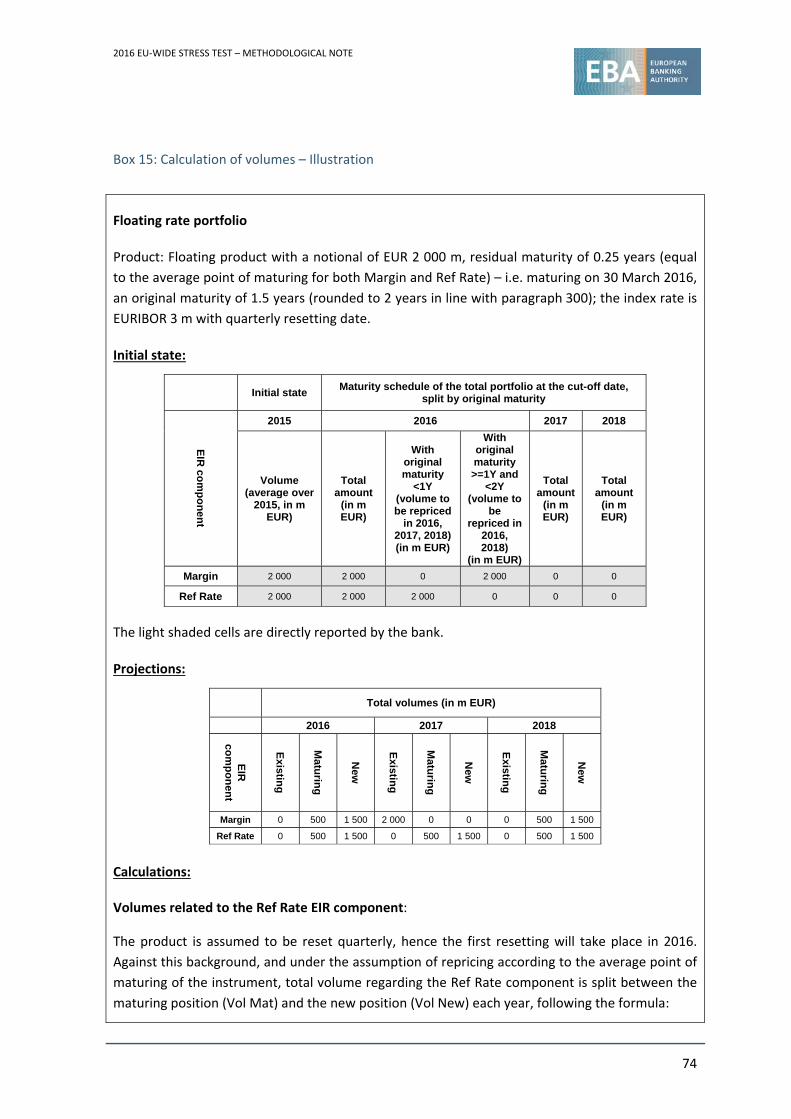
2016 EU‐WIDE STRESS TEST – METHODOLOGICAL NOTE
74
Box 15: Calculation of volumes – Illustration
Floating rate portfolio
Product: Floating product with a notional of EUR 2 000 m, residual maturity of 0.25 years (equal
to the average point of maturing for both Margin and Ref Rate) – i.e. maturing on 30 March 2016,
an original maturity of 1.5 years (rounded to 2 years in line with paragraph 300); the index rate is
EURIBOR 3 m with quarterly resetting date.
Initial state:
Initial state
Maturity schedule of the total portfolio at the cut-off date, split by original maturity
EIR
com
po
nen
t
2015 2016 2017 2018
Volume (average over
2015, in m EUR)
Total amount
(in m EUR)
With original maturity
<1Y (volume to be repriced
in 2016, 2017, 2018)(in m EUR)
With original maturity >=1Y and
<2Y (volume to
be repriced in
2016, 2018)
(in m EUR)
Total amount
(in m EUR)
Total amount
(in m EUR)
Margin 2 000 2 000 0 2 000 0 0
Ref Rate 2 000 2 000 2 000 0 0 0
The light shaded cells are directly reported by the bank.
Projections:
Total volumes (in m EUR)
2016 2017 2018
EIR
co
mp
on
ent
Existin
g
Matu
ring
Ne
w
Existin
g
Matu
ring
Ne
w
Existin
g
Matu
ring
Ne
w
Margin 0 500 1 500 2 000 0 0 0 500 1 500
Ref Rate 0 500 1 500 0 500 1 500 0 500 1 500
Calculations: Volumes related to the Ref Rate EIR component:
The product is assumed to be reset quarterly, hence the first resetting will take place in 2016.
Against this background, and under the assumption of repricing according to the average point of
maturing of the instrument, total volume regarding the Ref Rate component is split between the
maturing position (Vol Mat) and the new position (Vol New) each year, following the formula:
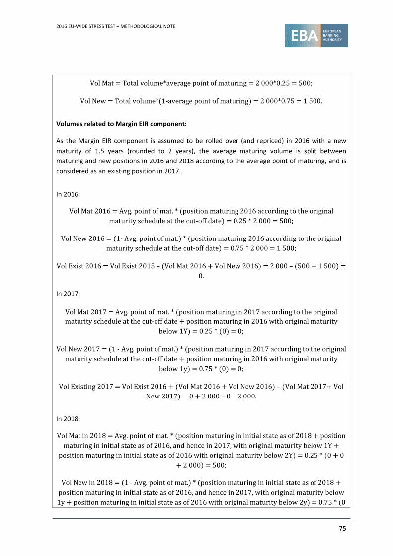
2016 EU‐WIDE STRESS TEST – METHODOLOGICAL NOTE
75
VolMat Totalvolume*averagepointofmaturing 2 000*0.25 500;
VolNew Totalvolume* 1‐averagepointofmaturing 2000*0.75 1500.
Volumes related to Margin EIR component:
As the Margin EIR component is assumed to be rolled over (and repriced) in 2016 with a new
maturity of 1.5 years (rounded to 2 years), the average maturing volume is split between
maturing and new positions in 2016 and 2018 according to the average point of maturing, and is
considered as an existing position in 2017.
In 2016:
VolMat2016 Avg.pointofmat.* positionmaturing2016accordingtotheoriginalmaturityscheduleatthecut‐offdate 0.25*2000 500;
VolNew2016 1‐Avg.pointofmat. * positionmaturing2016accordingtotheoriginalmaturityscheduleatthecut‐offdate 0.75*2000 1500;
VolExist2016 VolExist2015– VolMat2016 VolNew2016 2000– 500 1500 0.
In 2017:
VolMat2017 Avg.pointofmat.* positionmaturingin2017accordingtotheoriginalmaturityscheduleatthecut‐offdate positionmaturingin2016withoriginalmaturity
below1Y 0.25* 0 0;
VolNew2017 1‐Avg.pointofmat. * positionmaturingin2017accordingtotheoriginalmaturityscheduleatthecut‐offdate positionmaturingin2016withoriginalmaturity
below1y 0.75* 0 0;
VolExisting2017 VolExist2016 VolMat2016 VolNew2016 – VolMat2017 VolNew2017 0 2000–0 2000.
In 2018:
VolMatin2018 Avg.pointofmat.* positionmaturingininitialstateasof2018 positionmaturingininitialstateasof2016,andhencein2017,withoriginalmaturitybelow1Y
positionmaturingininitialstateasof2016withoriginalmaturitybelow2Y 0.25* 0 02000 500;
VolNewin2018 1‐Avg.pointofmat. * positionmaturingininitialstateasof2018 positionmaturingininitialstateasof2016,andhencein2017,withoriginalmaturitybelow1y positionmaturingininitialstateasof2016withoriginalmaturitybelow2y 0.75* 0
2016 EU‐WIDE STRESS TEST – METHODOLOGICAL NOTE
76
0 2000 1 500;
VolExist2018 VolExist2017 VolMat2017 VolNew2017 – VolMat2018 VolNew2018 2000 0–2000 0.
Fixed‐rate portfolio
For fixed‐rate portfolios, the calculation of existing, maturing and new volumes related to the
Margin EIR component is similar to the floating rate portfolio. The mechanism for the volumes
with regard to the Ref Rate EIR component, however, is different from that applied for floating
rate products: as reference rate and margin are expected to reprice at the same time, volumes for
reference rate are set equal to the volumes calculated for the Margin EIR component of the
relevant instrument.
4.3.1 Curve and currency shocks
304. Where required, banks should only use linear interpolation to add tenors to the provided
interest rate curves in the macro‐financial scenario. In line with paragraph 199, for tenors that
are shorter or longer than the range of tenors available in the scenario, the shocks to the
shortest and longest tenor available respectively should be applied as floors. Currencies should
be stressed independently, based on the curves provided for each currency in the scenario. For
currencies where no stress is provided, banks should generate their own curves consistent
with the macro‐financial scenario and provide justification for this expansion.
4.3.2 Reporting requirements
305. Starting point positions and projected positions, as well as the NII impact based on the
approach described in this section, shall be reported on the NII template (CSV_NII). Additional
historical (2011 to 2015) NII information on interest income and expenses, as well as historical
(2011 to 2015) and projected (2016 to 2018) discount unwinding, shall be reported on the NII
summary template (CSV_NII_SUM).
306. Banks are requested to report volumes and project the interest rates earned (or paid) of all
their assets and liabilities (including derivatives) split into the margin and reference rate
components with the exception of defaulted assets, for which the projected EIR will be
reported entirely as margin at total group level and also at country/currency level.
307. For the country/currency breakdown in the templates, banks shall report the country of the
location of the activity for all assets and liabilities, with the exception of exposures towards
sovereigns, for which banks will report the country of residence of the counterparty. The
number of country/currency pairs reported will be subject to the materiality thresholds
specified in Box 16. First, banks will be requested to limit their reporting to the most significant
country/currency pairs. Second, banks whose activities are heavily focused on their domestic
market and currency will not be requested to provide this additional information. Intra‐group
transactions shall not be included in the reporting by country/currency.

2016 EU‐WIDE STRESS TEST – METHODOLOGICAL NOTE
77
Box 16: Application of the materiality constraint on the currency/country breakdown requested
The following algorithm should be followed to determine the materiality of the country/currency
breakdown:
i. For each couple of country/currency, banks must compute the maximum
between the notional amount of total assets and total liabilities, excluding (only
for the purpose of ranking the country/currency couple) the notional amount of
derivatives. This will define the volume associated with each country/currency
couple;
ii. Banks must rank the country/currency couple according to their volume;
iii. Banks are requested to report the country/currency breakdown, either:
o Up to a 90% coverage of the sum of all country/currency volumes; or
o Up to 15 country/currency couples.
Domestic banks – i.e. banks whose non‐domestic exposures are less than 10% of the sum of
domestic and non‐domestic country exposures, and whose foreign currency exposures are less
than 10% of the sum of domestic and foreign currency exposures – are not requested to report
any country/currency breakdown but need to only report the results at the banking group level.
4.4 Impact on P&L
4.4.1 High‐level constraints on NII
308. Assumptions underlying the scenarios cannot lead (at group level) to an increase in the
bank’s NII, compared with the 2015 value, neither under the baseline nor the adverse
scenarios.
309. Under the adverse scenario banks’ interest expenses cannot decline at group level with
respect to the 2015 value.
2016 EU‐WIDE STRESS TEST – METHODOLOGICAL NOTE
78
4.4.2 Interest on defaulted loans
310. Under the baseline scenario, banks are required to project the interest accrued on
defaulted loans in line with their standing accounting practice (e.g. no recognition of unpaid
income, where only cash interest received is treated as income). Under the adverse scenario,
income on defaulted assets should not be recognised, with the exception of income from
discount unwinding,12 whose treatment is detailed in Box 17 below.
Box 17: Treatment of discount unwinding
Banks are entitled to recognise the interest income arising from discount unwinding; however,
they should take due account of the stress applied to their credit portfolio – in particular, the
stress on the LGD for the stock of defaulted assets and the increase in the stock of defaulted
assets. Against this background, banks are asked to provide their own projections of interest
income from discount unwinding, subject, under the adverse scenario, to the simplified constraint
below:
IIunwind t IIunwind t0 xMin 1, DefStock t /DefStock t0 * 1‐Provisions t /DefStock t / 1‐Provisions t0 /DefStock t0 .
Where:
IIunwind t stands for the interest income from discount unwinding for a given portfolio for
the time interval t;
Def Stock (t) stands for the notional value of the stock of defaulted assets for the time interval
t;
Provisions t stands for provisions for defaulted assets for the time interval t;
t0 stands for the year preceding the stress test time horizon.
The above constraint should be applied at bank level. It requires banks to reduce the interest
income stemming from discount unwinding proportionally to the increase in the stock of
provisions of their credit exposures, while allowing them to recognise more discount unwinding
effects due to the increase in the stock of defaulted assets. In addition, income stemming from
discount unwinding cannot exceed the income recognised at the cut‐off date.
311. Banks will be allowed to recognise income from discount unwinding only if this source of
income was clearly reported in their financial statements or, alternatively, they will need to
12 For the definition of discount unwinding, please refer to IAS 39, AG 93.
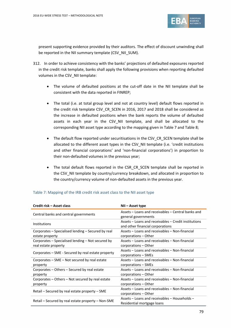
2016 EU‐WIDE STRESS TEST – METHODOLOGICAL NOTE
79
present supporting evidence provided by their auditors. The effect of discount unwinding shall
be reported in the NII summary template (CSV_NII_SUM).
312. In order to achieve consistency with the banks’ projections of defaulted exposures reported
in the credit risk template, banks shall apply the following provisions when reporting defaulted
volumes in the CSV_NII template:
The volume of defaulted positions at the cut‐off date in the NII template shall be
consistent with the data reported in FINREP;
The total (i.e. at total group level and not at country level) default flows reported in
the credit risk template CSV_CR_SCEN in 2016, 2017 and 2018 shall be considered as
the increase in defaulted positions when the bank reports the volume of defaulted
assets in each year in the CSV_NII template, and shall be allocated to the
corresponding NII asset type according to the mapping given in Table 7 and Table 8;
The default flow reported under securitisations in the CSV_CR_SCEN template shall be
allocated to the different asset types in the CSV_NII template (i.e. ‘credit institutions
and other financial corporations’ and ‘non‐financial corporations’) in proportion to
their non‐defaulted volumes in the previous year;
The total default flows reported in the CSR_CR_SCEN template shall be reported in
the CSV_NII template by country/currency breakdown, and allocated in proportion to
the country/currency volume of non‐defaulted assets in the previous year.
Table 7: Mapping of the IRB credit risk asset class to the NII asset type
Credit risk – Asset class NII – Asset type
Central banks and central governments Assets – Loans and receivables – Central banks and general governments
Institutions Assets – Loans and receivables – Credit institutions and other financial corporations
Corporates – Specialised lending – Secured by real estate property
Assets – Loans and receivables – Non‐financial corporations – Other
Corporates – Specialised lending – Not secured by real estate property
Assets – Loans and receivables – Non‐financial corporations – Other
Corporates – SME ‐ Secured by real estate property Assets – Loans and receivables – Non‐financial corporations – SMEs
Corporates – SME – Not secured by real estate property
Assets – Loans and receivables – Non‐financial corporations – SMEs
Corporates – Others – Secured by real estate property
Assets – Loans and receivables – Non‐financial corporations – Other
Corporates – Others – Not secured by real estate property
Assets – Loans and receivables – Non‐financial corporations – Other
Retail – Secured by real estate property – SME Assets – Loans and receivables – Non‐financial corporations – Other
Retail – Secured by real estate property – Non‐SME Assets – Loans and receivables – Households –Residential mortgage loans

2016 EU‐WIDE STRESS TEST – METHODOLOGICAL NOTE
80
Credit risk – Asset class NII – Asset type
Retail – Qualifying revolving Assets – Loans and receivables – Households – Other
Retail – Other retail – SME Assets – Loans and receivables – Non‐financial corporations – Other
Retail – Other retail – Non‐SME Assets – Loans and receivables – Households – Other
Equity Assets – Other assets
Securitisation Assets – Debt securities – Credit institutions and other financial corporations/assets – Debt securities – Non‐financial corporations
Other non‐credit obligation assets Assets – Other assets
Table 8: Mapping of the STA credit risk asset class to the NII asset type
Credit risk – Asset class NII – Asset type
Central governments or central banks Assets – Loans and receivables – Central banks and general governments
Regional governments or local authorities Assets – Loans and receivables – Central banks and general governments
Public sector entities Assets – Loans and receivables – Central banks and general governments
Multilateral development banks Assets – Loans and receivables – Credit Institutions
International organisations Assets – Loans and receivables – Central banks and general governments
Institutions Assets – Loans and receivables – Credit institutions and other financial corporations
Corporates – SME Assets – Loans and receivables – Non‐financial corporations – SMEs
Corporates – Non‐SME Assets – Loans and receivables – Non‐financial corporations – Other
Retail – SME Assets – Loans and receivables – Non‐financial corporations – SMEs
Retail – Non‐SME Assets – Loans and receivables – Households – Other
Secured by mortgages on immovable property –SME
Assets – Loans and receivables – Non‐financial corporations
Secured by mortgages on immovable property –Non‐SME
Assets – Loans and receivables – Households –Residential mortgage loans
Items associated with particularly high risk Assets – Other assets
Covered bonds Assets – Debt securities – Credit institutions and other financial corporations/assets – Debt securities – Non‐financial corporations
Claims on institutions and corporates with a ST credit assessment
Assets – Loans and receivables – Credit institutions and other financial corporations/assets – Loans and receivables – Non‐financial corporations – Other
Collective investments undertakings (CIUs) Assets – Other assets
Equity Assets – Other assets
Securitisation Assets – Debt securities – Credit institutions and other financial corporations/assets – Debt securities – Non‐financial corporations
Other exposures Assets – Other assets
2016 EU‐WIDE STRESS TEST – METHODOLOGICAL NOTE
81
4.4.3 Projection of the components of the EIR
313. Banks will use their own methodology to project their interest expenses and interest
income. In their projections, they will take into account the assumptions given in the following
paragraphs.
314. For fixed‐rate products, the margin and reference rate are assumed to remain constant
until the contractual maturity. For floating rate products, it is assumed that the margin is
repriced at the contractual maturity of the instrument, while the reference rate component is
repriced whenever the index rate of the instrument resets according to the contractual
schedule.
315. For each time interval of the projections, banks are requested to provide separate
projections for the margin and reference rate components of the EIR. In addition, banks are
requested to provide a split of the EIR rates between existing, maturing and newly repriced
positions.
316. For fixed‐rate instruments/portfolios, banks will project the reference rate, applying the
general risk‐free yield curve used in analysis of interest rate risk in the banking book. The
reference rate should be calculated for the original maturity of the instrument using a yield
curve taken from the time of origination for the relevant currency. Examples of acceptable
reference rates are interest rate swaps, or, for reference rate tenors below 1 year, the
applicable rate on unsecured interbank transactions.
317. For floating rate products that are contractually linked to an index rate, banks will use the
index rate as the reference rate, which should evolve in line with the macro‐financial scenario.
In particular, the reference rate of the floating leg of interest rate swap should be the index
rate of the swap, while the reference rate of the fixed leg of the swap will be the fixing of the
swap itself (hence the margin on the fixed leg of the interest rate swap is zero).
318. For assets for which banks have the option to adjust the margin at their discretion prior to
the maturity of the instrument, it is assumed that banks do not exercise this option.
319. The change in the margin of repriced instruments will be subject to the so‐called pass‐
through constraints, which provide floors for interest‐bearing liabilities and caps for
interesting‐earning assets. These constraints do not apply to instruments prior to the
contractual maturity of the products. In particular, they are not relevant for floating rate
instruments whose reference rate is adjusted before the expiration of the instrument’s
contract (i.e. before the repricing of the margin).
320. Although no methodological constraints are imposed on the reference rate of repriced
instruments, it is expected that the change in the reference rate of repriced instruments is
consistent with the macro‐financial scenarios for risk‐free yield curves.
2016 EU‐WIDE STRESS TEST – METHODOLOGICAL NOTE
82
321. In order to be coherent with the static‐balance sheet assumption, banks need to ensure
that the projected deposit rate will not result in an outflow of deposits, i.e. the margin paid on
deposits should allow banks to maintain the volume of deposits under stress. This applies in
particular to zero interest rate deposits, for which banks shall not assume that zero interest
rates can be maintained under a rising rate and spread scenario.
322. The reference rate of sight deposits, which are not at variable rates is assumed constant
over the scenario, such that any change in interest income/expenses earned/paid on this
instrument should be recognised as a change in the margin of the deposits. Subject to this
restriction, it is recommended that banks use a reference rate of zero, and reflect interest rate
projections entirely in the margin component.
323. Concerning variable rate deposits, banks are expected to use internal characterisation
analysis to assess repricing in the projection of the reference rates, always based on the
reference rate shock as defined in the scenario. Margin projections, subject to the pass‐
through constraints, shall also be related to macroeconomic developments foreseen by the
stress‐test scenarios.
324. Reference rates of deposits with rates calculated using a regulatory defined formula shall
be calculated according to this formula. In this regard banks are required to provide
legal/regulatory evidence about the prescribed application of regulatory formulas. The margin
component should be zero, and should remain zero throughout the scenario (i.e. it will not be
subject to the pass‐through constraints).
325. While there is no explicit forecast of monetary policy in the stress test scenarios, banks are
expected to factor in the projected changes in short‐term market rates into the costs of central
bank funding. More specifically, banks are required to compute the spread between the
central bank rates and the relevant short‐term rates at the cut‐off, and apply it to the
projected path of expected reference market interest rates over the stress test time horizon as
provided by the scenario. In line with the static balance sheet assumption, the volume of
central bank funding is assumed to remain constant and central bank funding instruments are
rolled‐over into similar central bank instruments.
326. The impact of interest rate derivatives used for hedging interest rate risk should be
recognised in the NII templates by reporting the interest cash flow stemming for those
instruments in separate lines. For example, in the case of a 3‐year fixed‐rate loan with a
matching interest rate swap, the reference rate on the loan would be recognised as the 3‐year
relevant risk‐free rate at origination throughout the entire loan period, regardless of interest
rate movements. Here, the items in the derivative lines will represent both legs of the swap. In
this example, the fixed leg would be represented within the hedging derivatives’ liabilities,
with the floating leg within the hedging derivatives’ assets.
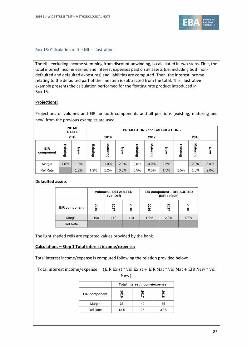
2016 EU‐WIDE STRESS TEST – METHODOLOGICAL NOTE
83
Box 18: Calculation of the NII – Illustration
The NII, excluding income stemming from discount unwinding, is calculated in two steps. First, the total interest income earned and interest expenses paid on all assets (i.e. including both non‐defaulted and defaulted exposures) and liabilities are computed. Then, the interest income relating to the defaulted part of the line item is subtracted from the total. This illustrative example presents the calculation performed for the floating rate product introduced in Box 15.
Projections:
Projections of volumes and EIR for both components and all positions (existing, maturing and
new) from the previous examples are used.
INITIAL STATE
PROJECTIONS and CALCULATIONS
2015 2016 2017 2018
EIR component
Existin
g
New
Existin
g
Matu
ring
New
Existin
g
Matu
ring
New
Existin
g
Matu
ring
New
Margin 1.0% 1.0% 1.0% 2.0% 2.0% 4.0% 2.5%
2.0% 3.0%
Ref Rate 1.2% 1.2% 1.2% 0.5% 0.5% 0.5% 1.5% 1.5% 1.5% 2.0%
Defaulted assets
Volumes – DEFAULTED
(Vol Def) EIR component – DEFAULTED
(EIR default)
EIR component
2016
2017
2018
2016
2017
2018
Margin 100 110 110 1.9% 2.2% 1.7%
Ref Rate
The light shaded cells are reported values provided by the bank.
Calculations – Step 1 Total interest income/expense:
Total interest income/expense is computed following the relation provided below:
Totalinterestincome/expense EIRExist*VolExist EIRMat*VolMat EIRNew*VolNew .
Total interest income/expense
EIR component
2016
2017
2018
Margin 35 40 55
Ref Rate 13.5 25 37.5
2016 EU‐WIDE STRESS TEST – METHODOLOGICAL NOTE
84
Calculations – Step 2 Impact on total interest income/expense of the defaulted assets:
Step 2a: Difference between the EIR component for the defaulted and the non‐defaulted asset
multiplied by the defaulted volume (split into existing and maturing)
The cells in the table are computed in the following way:
DiffExist EIRdefault‐EIRExist *VolDef;
DiffMat EIRdefault‐EIRMat *VolDef;
DiffNew EIRdefault–EIRNew *VolDef.
Step 2b: Subtracting the difference on interest between defaulted and non‐defaulted assets
The impact of defaulted assets is proportionally distributed among existing and defaulted assets
following the relation provided below:
Interestincome/expense TotalInterestincome/expense DiffExist*VolExist DiffMat*VolMat DiffNew*VolNew / VolExist VolMat VolNew .
a. Constraints on the margin component for liability positions
327. Under the baseline scenario, banks are required (at a minimum) to reflect a proportion of
the changes in the sovereign bond spread of the country of location of the activity in the
margin EIR component of their repriced liabilities. Under the adverse scenario, the margin paid
on interest‐bearing liabilities cannot increase less than the higher between a proportion of the
changes in the sovereign spread of the country of location of the activity and the same
proportion applied to the increase of an idiosyncratic component, derived from the impact on
banks’ wholesale funding rate of a rating downgrade as described in Box 19; the impact shall
be applied immediately at the beginning of the time horizon.
Box 19: Floor for the evolution of the margin paid on new liabilities (pass‐through constraint)
The Margin on banks’ new liabilities at time t is floored by:
MarginNewL t MarginNewL t0 γMax 0,ΔSovSpread t ,Δidiosyncraticcomponent .
Where:
Margin NewL t stands for the Margin EIR component on their repriced liabilities during
time interval t;
t0 stands for the year preceding the stress test horizon;

2016 EU‐WIDE STRESS TEST – METHODOLOGICAL NOTE
85
ΔSov Spread t is the change in the relevant sovereign spread – i.e. difference between the yield‐to‐maturity of the 10‐year sovereign’s debt security and the swap rate for the same
currency and maturity, between t and t0;
γ is a factor specific to the different types of liabilities, which reflects the heterogeneity in the
relationship between the sovereign spreads and the funding rates across different types of
liabilities as summarised in the table below:
Retail
deposits
– sight
Retail
deposits
– term
NFC
deposits
– sight
NFC
deposits
– term
Gov. and
central
banks
deposits
– sight
Gov. and
central
banks
deposits
– term
Deposits
from
credit
insti‐
tutions
and
other
financial
corpo‐
rations
Debt
securities
(excl.
covered
bonds)
Covered
bonds
Certifi‐
cates of
deposits
and
repos
γ 0.1 0.5 0.2 0.5 0.2 0.5 1 1 0.75 0.2
Δ idiosyncratic component stands for the impact on the idiosyncratic component. Under the
baseline scenario, the Δ idiosyncratic component will be 0; under the adverse scenario, it will
represent the expected change in the margin of senior unsecured debt, issued in the bank’s
country of origin or main country of funding, denominated in local currency with 5 years
residual maturity, in the event of an instantaneous External Credit Assessment Institution
(ECAI) credit rating downgrade (taking the rating as of end 2015 as the start point). Under the
adverse scenario, Δ idiosyncratic component shall be calculated as a single number per bank,
used for all liabilities in all countries/currencies and assumed constant over the scenario. The
idiosyncratic component is floored, under the adverse scenario, by the values listed below:
Credit rating (Standard & Poor’s classification) 31 December 2015
Shock to the idiosyncratic component (bps)
AAA 25
AA+ 30
AA 35
AA‐ 40
A+ 45
A 50
A‐ 60
BBB+ 70BBB 80
BBB‐ 95
BB+ 110
BB 125
BB‐ 145
B+ 165
B 185
B‐ 220
CCC+/CCC/CCC‐/CC+/CC/CC‐ 300
In order to apply the floor, and in cases where the bank has more than one rating from nominated
2016 EU‐WIDE STRESS TEST – METHODOLOGICAL NOTE
86
ECAIs, the following creiteria will apply:
Long‐term credit ratings will prevail over short‐term credit ratings;
Where two credit ratings are available from nominated ECAIs and the two correspond
to different impacts on the margin component of the EIR, the rating leading to a more
severe impact shall be chosen;
Where more than two credit ratings are available from nominated ECAIs, the two
ratings generating the two less severe impacts shall be referred to. Out of the two
preselected, the one with a higher impact will be chosen.
If the applicable rating is issued by a nominated ECAI other than S&P, the bank shall map it to one
of the ratings envisaged in the idiosyncratic component floor table. In this mapping, the following
constraint will apply: both ratings shall share the same credit quality step according to the Annex
III of the Joint final draft Implementing Technical Standards on the mapping of ECAIs’ credit
assessment under Article 136(1) and (3) of the (CRR).
Example: The shock to the idiosyncratic component for a bank with a credit rating of AA‐ as of end
2015 will be +40 bps over the entire stress test period under the adverse scenario. Similarly, the
shock to the idiosyncratic component for a bank with a credit rating of BB‐ as of end 2015 will be
145 bps under the adverse scenario.
328. The pass‐through constraint on the evolution of the EIR applies to all interest expense
positions, except derivatives instruments.
329. Any legally mandated restrictions to pass‐through mechanisms should be identified before
submission of the data and explained in accompanying documents. Discussions during the
quality assurance process may, in exceptional circumstances, lead to deviations from this rule.
b. Constraints on the margin component for asset positions
330. Under both the baseline and the adverse scenarios, banks are required to cap the margin
on their repriced assets by the sum of the margin starting value and a proportion of the
change in the sovereign bond spread in the country of exposure, as explained in Box 20.
331. Exceptional cases of legally prescribed funding matches between the assets and liabilities
sides may be identified as part of the quality assurance process, which would need to be taken
into account in the stress test when considering the application of the pass‐through
constraints.
2016 EU‐WIDE STRESS TEST – METHODOLOGICAL NOTE
87
Box 20: Cap on the evolution of the margin earned on new assets (pass‐through constraint)
The Margin EIR component on banks’ new repriced assets at time t is capped by:
MarginNewA t MarginNewA t0 λ Max ΔSovSpread t ,0 .
Where:
MarginNewA t stands for the Margin on the repriced assets in the time interval t;
t0 stands for the year preceding the stress test time horizon;
ΔSov Spread t is the change in the relevant sovereign spread – i.e. difference between the yield‐to‐maturity of the 10‐year sovereign’s debt security and the swap rate for the same
currency and maturity, between t and t0;
λ is a factor specific to the different types of assets under consideration, which reflects the
heterogeneity in the relationship between the sovereign spreads and the lending rates across
different types of assets as summarised in the table below:
Household – Residential mortgage
Household – Other
Financial corporations
Non‐financial corporations
Central bank Government
λ 0.15 0.15 0.5 0.15 0 1
332. These caps on pass‐through rates apply to all interest income earning positions except
derivative instruments.
2016 EU‐WIDE STRESS TEST – METHODOLOGICAL NOTE
88
5. Conduct risk and other operational risks
5.1 Overview
333. Banks shall project the P&L impact of losses arising from conduct risk and other operational
risks, using, when relevant, their internal models and, in the case of conduct risk, available
qualitative information.
334. Banks shall also project capital requirements for operational risk within the time horizon of
the exercise.
335. Banks’ projections are subject to the constraints summarised in Box 21.
Box 21: Summary of the constraints on banks’ projections of conduct risk and other operational
risks
Projections of losses that may arise from new conduct risk events are subject to a
minimum floor, computed in the baseline scenario as the average of the historical conduct
risk losses reported by the bank during the 2011‐2015 period for non‐material events only
– i.e. excluding past losses of historical material conduct risk events reported during this
period. This floor is more conservative under the adverse scenario and requires the banks
to apply a stress multiplier to the average (paragraph 373);
Projections of losses due to other operational risks are subject to a minimum floor,
computed under the baseline scenario as the average of other historical operational risk
losses reported by the bank during the 2011‐2015 period times a multiplier. This floor is
more conservative in the adverse scenario and requires banks to apply a stress multiplier
to the average (paragraph 378);
Total capital requirements for operational risk in each year of the projection horizon shall
not fall below the actual minimum capital requirements for operational risk reported by
the bank at the beginning of the exercise (paragraph 381).
2016 EU‐WIDE STRESS TEST – METHODOLOGICAL NOTE
89
5.2 Scope
336. The scope of the operational risk stress is defined to cover the impact on the P&L of
potential future losses arising from conduct risk and other operational risks. This also covers
the effect of the stress on operational risk capital requirements.
5.3 High‐level assumptions and definitions
5.3.1 Definitions
337. Banks are required to apply consistent definitions for the following items.
338. Conduct risk is defined as the current or prospective risk of losses to an institution arising
from an inappropriate supply of financial services, including cases of wilful or negligent
misconduct. Banks shall refer to paragraphs 253–257 of the EBA Guidelines on common
procedures and methodologies for the SREP. For the purpose of reporting historical data and
projections in the stress test templates, conduct risk losses will be approximated by banks to
event type 4 (‘clients, products and business practices’) and event type 1 (‘internal fraud’) of
the COREP template for operational risk (C 17.00). Institutions shall justify the exclusion from
the consideration as conduct risk of any event classified as event type 1 or 4. In addition, banks
shall report as conduct risk any events that match the definition provided, even if they are
reported as an event type other than 1 or 4 of the above‐mentioned COREP template,
providing evidence to the competent authority that justifies this classification.
339. Other operational risk is defined as the risk of losses according to the definition provided in
the CRR (i.e. ‘operational risk’ means the risk of losses resulting from inadequate or failed
internal processes, people and systems or from external events, and includes legal risk), but
excluding all conduct‐related losses. For the purpose of reporting historical data and
projections in the stress test templates, banks will consider as other operational risk all event
types that are not defined as conduct risk events above.
340. A historical material conduct risk event is defined as any misconduct issue that has
triggered aggregate gross losses greater than 10 bps of the end‐2015 CET1 capital of the
institution at a consolidated level during the period 2011‐2015.
341. A new conduct risk event is defined as a misconduct issue that, as of the start of the
exercise (31 December 2015), is unknown to the bank or is already known but has had no
material P&L impact (below 10 bps of the end‐2015 CET1 capital of the institution at a
consolidated level) during the 2011‐2015 period. In this context, new known conduct risk
events are material if the firm expects the event to trigger gross losses greater than 10 bps of
the end‐2015 CET1 capital of the institution at a consolidated level during the 3 years of the
exercise.
342. Number of loss events is defined as the number of operational risk events accounted for
the first time in the P&L statement within the reporting period (2011‐2015 for actual data and
2016 EU‐WIDE STRESS TEST – METHODOLOGICAL NOTE
90
2016‐2018 for projections). In the case of loss adjustments within the reporting period, no
additional numbers of loss events should be reported.
343. Recovery is defined as an independent occurrence related to the original operational risk
loss that is separate in time, in which funds or inflows of economic benefits are received from
first or third parties, such as insurers or other parties.
344. Gross loss is defined as a loss stemming from an operational risk event or event type before
recoveries of any type.
345. Rapidly recovered loss event is defined as an operational risk event that leads to losses
that are partly or fully recovered within five working days. In case of a rapidly recovered loss
event, only the part of the loss that is not fully recovered (i.e. the loss net of the partial rapid
recovery) should be considered and reported as gross loss.
346. Date of accounting is defined as the date when an operational risk gross loss or
reserve/provision was accounted for the first time in the P&L statement.
347. Total loss recovery is defined as the sum of the recoveries accounted for within the
reporting period, relevant to loss events included into the ‘total amount of gross losses’.
348. The relevant indicator (RI) is defined as in Article 316 of the CRR.
5.3.2 Reporting requirements
349. All banks are required to report historical data on incurred gross losses on conduct risk and
other operational risks on a yearly basis from 2011 to 2015 in the general operational risk
template (CSV_OR_GEN) at a consolidated level, irrespective of the operational risk approach
applied.
350. Banks shall report, in each year of the reporting period, the total amount of gross losses
resulting from the sum of the following elements:
The gross loss amounts equal or larger than EUR 10 000, corresponding to operational
risk events accounted for the first time in the P&L during that specific year, within the
reporting period (2011‐2015), irrespective of when they have occurred and;
The net loss adjustments arising e.g. from additional settlements, increases of
provisions, and releases of provisions with accounted during that year and that are
equal or larger than EUR 10 000, corresponding to operational risk events accounted
for the first time later than January 2005.
351. In those cases where capital requirements are modelled using AMA or standardised
approaches, banks will report historical data on incurred gross losses for conduct risk and
other operational risks by loss‐size‐based buckets (minimum size is EUR 10 000) in
CSV_OR_GEN. They shall report such data under the constraint that the threshold for internal
2016 EU‐WIDE STRESS TEST – METHODOLOGICAL NOTE
91
data collection is EUR 10 000 (or the equivalent, applying an FX rate at the time of recording
the loss) and it is homogeneous across operational risk categories. Historical material conduct
risk events will be reported separately in CSV_OR_CON. Banks shall group all payments
relating to the same material conduct risk event for the purpose of populating both
CSV_OR_GEN and CSV_OR_CON (thus ensuring that material conduct risk events comprising a
large number of small items are appropriately captured).
352. Banks applying the basic indicator approach are also expected to report yearly operational
risk‐incurred losses from 2011‐2015 in CSV_OR_GEN, with a split between conduct risk and
other operational risks but without further details per loss‐size‐based buckets. Historical
material conduct risk events shall be reported separately in CSV_OR_CON by these banks as
well, when relevant.
353. In the case of events with a lifespan of over several years, the initial impact and/or the net
loss adjustments should be reported in the pertinent years of accounting. The sum of the
initial impact and/or net loss adjustments accounted during the reporting period (2011‐2015)
will determine the total size of the event for the purpose of classifying it as material or not
material, as well for reporting its amounts (i.e. initial impact and/or loss adjustments) in the
relevant loss‐size‐based bucket. If e.g. in 2011 the event happens with a n initial loss of EUR
15,000, then in 2012 an additional provisison is booked of EUR 50,000 for the same event, in
2013 another provision of EUR 200,000 is booked for the same event and finally in 2014 a
further provision of EUR 30,000 is again booked for the same event, the bank should report
this event as follows, in accordance with the COREP instructions:
in 2011, EUR 15,000 in the bucket ‘≥ EUR 10,000 and < EUR 20,000’;
in 2012, EUR 50,000 in the bucket ‘≥ EUR 20,000 and < EUR 100,000’;
in 2013, EUR 200,000 in the bucket ‘≥ EUR 100,000 and < EUR 1,000,000’;
in 2014, EUR 30,000 in the bucket ‘≥ EUR 100,000 and < EUR 1,000,000’.
354. In the case of a rapidly recovered loss event, only the part of the loss that is not fully
recovered (i.e. the loss net of the partial rapid recovery) should be considered and reported as
gross loss.
355. In case of a common operational risk event or multiple events linked to an initial
operational risk event generating several events or losses, the related losses should be
grouped and entered into the template as a single loss. The bank should report one event in
case of a common operational risk event and/or the number of the several events linked to the
root event, in case of multiple events.
356. In accordance with Article 322(3)(b) of the CRR, operational risk losses that are related to
market risk shall be included in the operational risk templates, while operational risk losses
that are related to credit risk shall be excluded.
2016 EU‐WIDE STRESS TEST – METHODOLOGICAL NOTE
92
357. When reporting the gross losses, banks will include the following items, in accordance with
letters (a), (b), (c) and (f) of Article 28 of the EBA Final Draft RTS on AMA assessment
(EBA/RTS/2015/02):
Direct charges, including impairments and settlement charges, to the P&L and write‐
downs due to the operational risk event;
Costs incurred as a consequence of the operational risk event, including: external
expenses with a direct link to the operational risk event (such as legal expenses and
fees paid to advisors, attorneys or suppliers), and costs of repair or replacement to
restore the position prevailing before the operational risk event;
Provisions or reserves accounted for in the P&L statement against probable
operational risk losses;
Timing losses13.
358. When determining the scope of the gross losses to be reported, banks should also consider
the provisions included in Articles 29(3), 29(4) and 29(6) of the Final draft RTS on AMA
assessment.
359. Banks are also requested to provide, in the CSV_OR_GEN template, data on the number of
loss events, on total loss recovery and on the relevant indicator.
360. The quality assurance by supervisors of banks’ projections is of special relevance in the case
of conduct risk, given the high variability of the potential outcomes of the issues when settled,
especially the material ones. Banks should support their projections for material conduct risk
events with all available evidence, both quantitative and qualitative. Banks may also be asked
by their competent authorities to provide evidence regarding issues that are widespread in the
industry and have resulted in losses for other institutions, which could be of relevance for
them based on their business activities. When quality assuring bank’s projections, competent
authorities will take into account not only their supervisory knowledge of the particular bank,
but also a comparison to the sector and the impact of similar issues in the bank’s peer group.
5.4 Impact on P&L
5.4.1 Conduct risk treatment
361. Banks will stress their conduct risk losses by applying either a qualitative or a quantitative
approach according to the instructions below. In both cases, a minimum floor for new non‐
material conduct risk losses will apply.
13 For the definition of timing losses please refer to the EBA/RTS/2015/02 Article 1(f).
2016 EU‐WIDE STRESS TEST – METHODOLOGICAL NOTE
93
362. Under both approaches, the P&L impact of banks’ conduct risk estimates will be included in
‘gains or losses arising from operational risk’ in the P&L template (CSV_P&L), taking into
account the applicable floor.
363. Institutions will apply the qualitative approach when they report any historical material
conduct risk event during the period 2011‐2015. Institutions reporting no historical material
conduct risk event during 2011‐2015 will also apply the qualitative approach if new material
events are expected, or if the relevant competent authority deems it necessary based on their
knowledge of the bank and on their supervisory judgment (if they deem that the institution
may face any new material conduct risk event in the future).
364. All remaining institutions will apply the quantitative approach.
a. Qualitative approach to estimating future conduct risk losses
365. Banks applying the qualitative approach shall:
Report historical data on incurred gross losses on conduct risk in the general template
(CSV_OR_GEN) as indicated in paragraphs 349 to 352 above. In the same template
they will report projections of losses for non‐material events during the time horizon
of the exercise;
Identify and report (separately) historical material conduct risk events in the conduct
risk template (CSV_OR_CON), including an estimate of all potential losses that may
still arise from them, in excess of accounting provisions and losses already booked by
December 2015, during the time horizon of the exercise. This is applicable for both
the baseline and the adverse scenarios;
Include, in the conduct risk template (CSV_OR_CON), a projection of potential losses
that may arise from new material conduct risk events during the time horizon of the
exercise, both under the baseline and the adverse scenarios.
366. Banks shall report individually in the CSV_OR_CON the 25 largest historical material events
in terms of aggregate projected losses, and also the 25 largest new material events in terms of
aggregate projected losses. The rest of material events not included among the 25 historical
largest and/or the 25 new largest (if any) shall be reported jointly in a different single row for
historical events and in another single row for new events.
367. Banks’ estimates of future conduct costs linked to historical material conduct risk events or
new conduct risk events reported in the conduct risk template (CSV_OR_CON) shall be
determined, irrespective of whether a provision has been recognised, by evaluating a range of
settlement outcomes for each issue and assigning probabilities to these outcomes. Adverse
outcomes should be attributed higher probabilities under the adverse scenario compared to
the baseline scenario, so that banks should have a high level of confidence that, under the
adverse scenario, the losses would not exceed the loss estimate for material conduct risk

2016 EU‐WIDE STRESS TEST – METHODOLOGICAL NOTE
94
events. These estimates are expected to exceed provisions, except for events where there is a
high degree of certainty regarding the eventual cost.
368. When projecting conduct risk losses linked to historical material conduct risk events and
new conduct risk events, banks will consider the time dimension and report the projected loss
in the year that the settlement of the misconduct issue will most likely occur. If there is
uncertainty on when the issue will be settled, then banks should prorate the projected loss
over the 3 years of the exercise.
369. Table 9 below provides an illustration on the approach to follow in order to project conduct
risk losses in the adverse scenario.
Table 9: Projection of conduct risk losses under the qualitative approach and in the adverse
scenario – Illustration
Existing treatment of the misconduct issue Possible approach to projecting future conduct risk losses
An accounting provision has been raised. There is a high degree of certainty over the eventual cost.
The estimate will equal the existing provisions.
An accounting provision has been raised. There is a high degree of uncertainty over the eventual settlement cost. While the IAS 37 provision strikes a balance between potential upside and downside, the likelihood of adverse outcomes exceeding existing provisions is greater rather than remote.
The estimate should exceed the existing provision. Banks are expected to provide an estimate, even if they are unable to reliably quantify the full range of potential outcomes, by exercising expert judgement and targeting a high level of confidence of settling at or below their estimate.
An accounting provision has not been raised. While a settlement cost is not probable, there is sufficient evidence to determine a range of settlement outcomes, and the possibility of a significant settlement cost is greater than remote.
An estimate should be determined by evaluating a range of settlement outcomes and assigning probabilities to these outcomes. In the adverse scenario, banks should have a high level of confidence that the loss would not exceed the loss estimate for material conduct risk events. Adverse outcomes should be attributed higher probabilities under the adverse scenario compared to the baseline scenario.
An accounting provision has not been raised. While a possible obligation has been identified, current evidence is insufficient to be able to reliably quantify any potential liability, or range of liabilities, that may exist. The possibility of a significant settlement cost is greater than remote.
An estimate should be determined by exercising expert judgement and targeting a high level of confidence of settling at or below the estimate.
370. Banks shall provide supervisors with any information – both quantitative and qualitative –
they have used in forming this assessment. This information shall include the extent of their
business in relevant areas.
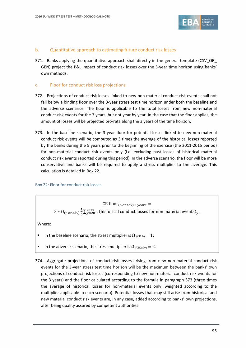
2016 EU‐WIDE STRESS TEST – METHODOLOGICAL NOTE
95
b. Quantitative approach to estimating future conduct risk losses
371. Banks applying the quantitative approach shall directly in the general template (CSV_OR_
GEN) project the P&L impact of conduct risk losses over the 3‐year time horizon using banks’
own methods.
c. Floor for conduct risk loss projections
372. Projections of conduct risk losses linked to new non‐material conduct risk events shall not
fall below a binding floor over the 3‐year stress test time horizon under both the baseline and
the adverse scenarios. The floor is applicable to the total losses from new non‐material
conduct risk events for the 3 years, but not year by year. In the case that the floor applies, the
amount of losses will be projected pro‐rata along the 3 years of the time horizon.
373. In the baseline scenario, the 3 year floor for potential losses linked to new non‐material
conduct risk events will be computed as 3 times the average of the historical losses reported
by the banks during the 5 years prior to the beginning of the exercise (the 2011‐2015 period)
for non‐material conduct risk events only (i.e. excluding past losses of historical material
conduct risk events reported during this period). In the adverse scenario, the floor will be more
conservative and banks will be required to apply a stress multiplier to the average. This
calculation is detailed in Box 22.
Box 22: Floor for conduct risk losses
CR floor ,
3 ∗ Ω ∑ historicalconductlossesfornonmaterialevents .
Where:
In the baseline scenario, the stress multiplier is Ω CR,b 1;
In the adverse scenario, the stress multiplier is Ω CR, adv 2.
374. Aggregate projections of conduct risk losses arising from new non‐material conduct risk
events for the 3‐year stress test time horizon will be the maximum between the banks’ own
projections of conduct risk losses (corresponding to new non‐material conduct risk events for
the 3 years) and the floor calculated according to the formula in paragraph 373 (three times
the average of historical losses for non‐material events only, weighted according to the
multiplier applicable in each scenario). Potential losses that may still arise from historical and
new material conduct risk events are, in any case, added according to banks’ own projections,
after being quality assured by competent authorities.
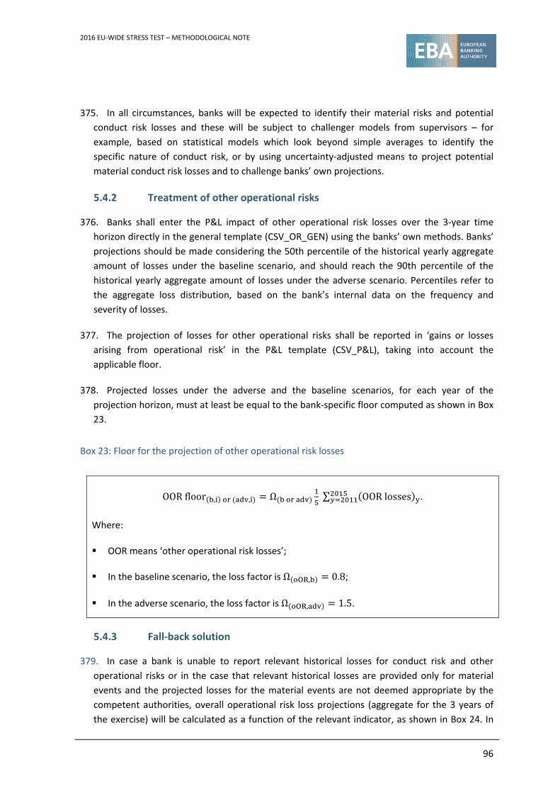
2016 EU‐WIDE STRESS TEST – METHODOLOGICAL NOTE
96
375. In all circumstances, banks will be expected to identify their material risks and potential
conduct risk losses and these will be subject to challenger models from supervisors – for
example, based on statistical models which look beyond simple averages to identify the
specific nature of conduct risk, or by using uncertainty‐adjusted means to project potential
material conduct risk losses and to challenge banks’ own projections.
5.4.2 Treatment of other operational risks
376. Banks shall enter the P&L impact of other operational risk losses over the 3‐year time
horizon directly in the general template (CSV_OR_GEN) using the banks’ own methods. Banks’
projections should be made considering the 50th percentile of the historical yearly aggregate
amount of losses under the baseline scenario, and should reach the 90th percentile of the
historical yearly aggregate amount of losses under the adverse scenario. Percentiles refer to
the aggregate loss distribution, based on the bank’s internal data on the frequency and
severity of losses.
377. The projection of losses for other operational risks shall be reported in ‘gains or losses
arising from operational risk’ in the P&L template (CSV_P&L), taking into account the
applicable floor.
378. Projected losses under the adverse and the baseline scenarios, for each year of the
projection horizon, must at least be equal to the bank‐specific floor computed as shown in Box
23.
Box 23: Floor for the projection of other operational risk losses
OORfloor , , Ω ∑ OOR losses .
Where:
OOR means ‘other operational risk losses’;
In the baseline scenario, the loss factor is Ω , 0.8;
In the adverse scenario, the loss factor is Ω , 1.5.
5.4.3 Fall‐back solution
379. In case a bank is unable to report relevant historical losses for conduct risk and other
operational risks or in the case that relevant historical losses are provided only for material
events and the projected losses for the material events are not deemed appropriate by the
competent authorities, overall operational risk loss projections (aggregate for the 3 years of
the exercise) will be calculated as a function of the relevant indicator, as shown in Box 24. In
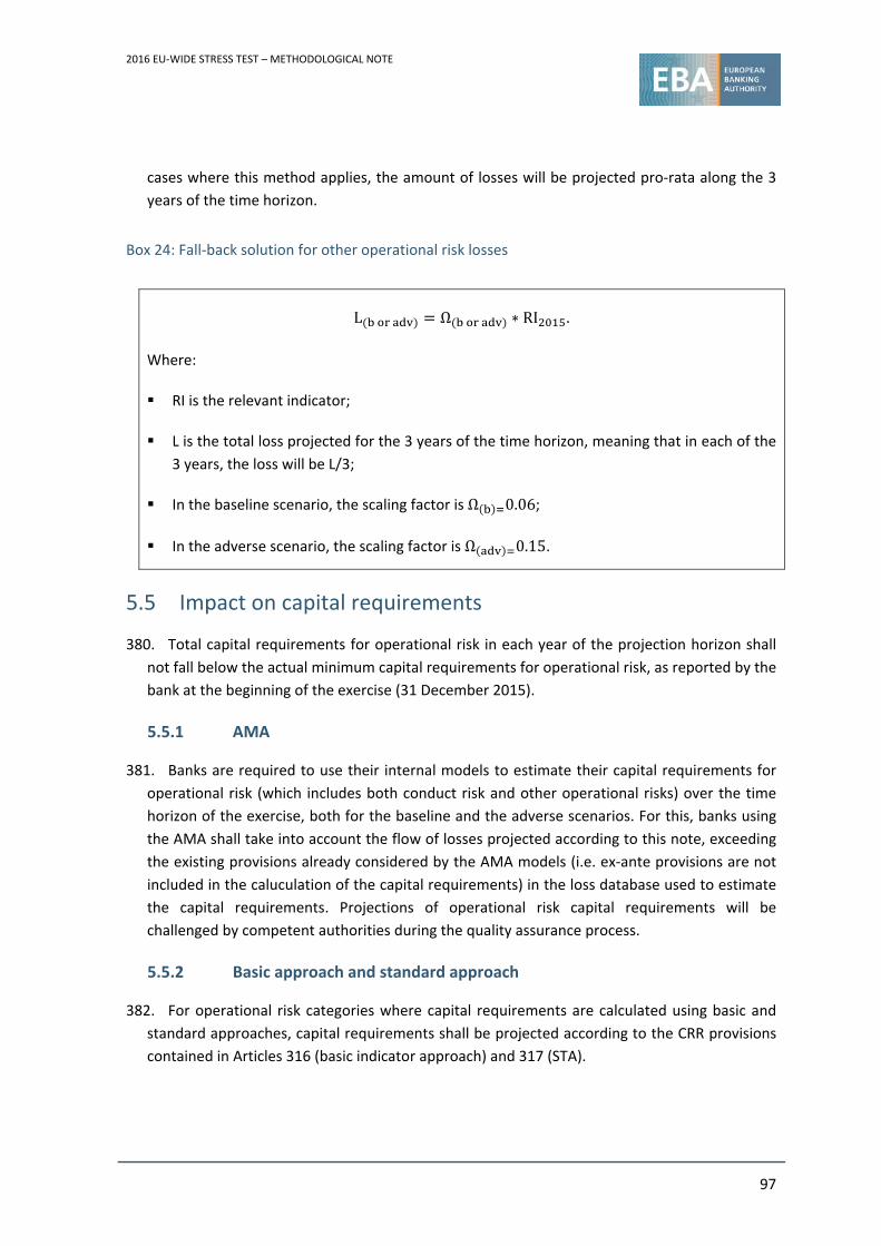
2016 EU‐WIDE STRESS TEST – METHODOLOGICAL NOTE
97
cases where this method applies, the amount of losses will be projected pro‐rata along the 3
years of the time horizon.
Box 24: Fall‐back solution for other operational risk losses
L Ω ∗ RI .
Where:
RI is the relevant indicator;
L is the total loss projected for the 3 years of the time horizon, meaning that in each of the
3 years, the loss will be L/3;
In the baseline scenario, the scaling factor is Ω 0.06;
In the adverse scenario, the scaling factor is Ω 0.15.
5.5 Impact on capital requirements
380. Total capital requirements for operational risk in each year of the projection horizon shall
not fall below the actual minimum capital requirements for operational risk, as reported by the
bank at the beginning of the exercise (31 December 2015).
5.5.1 AMA
381. Banks are required to use their internal models to estimate their capital requirements for
operational risk (which includes both conduct risk and other operational risks) over the time
horizon of the exercise, both for the baseline and the adverse scenarios. For this, banks using
the AMA shall take into account the flow of losses projected according to this note, exceeding
the existing provisions already considered by the AMA models (i.e. ex‐ante provisions are not
included in the caluculation of the capital requirements) in the loss database used to estimate
the capital requirements. Projections of operational risk capital requirements will be
challenged by competent authorities during the quality assurance process.
5.5.2 Basic approach and standard approach
382. For operational risk categories where capital requirements are calculated using basic and
standard approaches, capital requirements shall be projected according to the CRR provisions
contained in Articles 316 (basic indicator approach) and 317 (STA).
2016 EU‐WIDE STRESS TEST – METHODOLOGICAL NOTE
98
6. Non‐interest income, expenses and capital
6.1 Overview
383. A prescribed formula is applied to the main income items (i.e. dividend income and net fee
and commission income based on historical values relative to banks’ assets). Banks shall use
their own methodology to project their other non‐interest income and expenses items that are
not covered by credit risk, market risk or operational risk, both for the baseline and the
adverse scenarios. These projections are subject to the constraints summarised in Box 25. The
macroeconomic shocks and market risk methodology shall be applied for stressing real estate
assets and defined benefit pension plans, respectively.
Box 25: Summary of the constraints on banks’ projections of non‐interest income, expenses and
capital
For dividend and net fee and commission income, net income from each item has to
remain constant at the 2015 level in the baseline scenario. In the adverse scenario, the
minimum between the ratio of net income from each item over total assets in 2015 and
the average of the two years with the smallest ratios that occurred over the last 5 years
should be assumed (paragraph 395);
Administrative expenses and other operating expenses cannot fall below the value
observed in 2015 – unless an adjustment of this floor for one‐offs is permitted by the
competent authority. Likewise, profit or loss from discontinued operations are to be set at
zero for the stress test time horizon – unless an adjustment for one‐off is permitted
(paragraph 396);
Other operating income is capped at the 2015 value (paragraph 408);
A common tax rate of 30% shall be applied (paragraph 413).
No impact is assumed for realised gains or losses on financial assets and liabilities not
measured at fair value through P&L, gains or losses on derecognition of non‐financial
assets, or investments in subsidiaries, joint ventures and associates, negative goodwill,
impairments on goodwill, FX effects (paragraphs 391, 405, 406, 407, 409 and 411).
For dividends paid, under the baseline and the adverse scenarios, banks shall apply a pay‐
out ratio based on their publicly declared projected dividend policies. If no dividend policy
is available or documented, the bank shall apply the following rule. The pay‐out ratio in the
2016 EU‐WIDE STRESS TEST – METHODOLOGICAL NOTE
99
baseline should be the maximum between 30% and the median of the observed pay‐out
ratios in profitable years over the last 5 years. In the adverse scenario, the same amount of
dividends as in the baseline scenario shall be assumed, unless the bank can provide
evidence that it can deviate from this rule and the deviation is approved by the relevant
competent authority. In both cases, a zero dividend is accepted if the bank is loss‐making
(paragraph 403).
6.2 Scope
384. The projections of non‐interest income and expenses exclude any P&L positions and capital
impacts covered in the approaches for credit risk, market risk, operational risk or NII.
385. The following FINREP P&L items are part of non‐interest income and expenses:
i. Expenses on share capital repayable on demand;
ii. Dividend income;
iii. Fee and commission income, net;
iv. Gains (losses) on derocognition of financial assets and liabilities not measured at
fair value through profit and loss, net;
v. Exchange differences, net;
vi. Gains or losses on derecognition of non financial assets, net;
vii. Other operating income;
viii. Other operating expenses;
ix. Administrative expenses;
x. Depreciation;
xi. Impairment on non‐financial assets;
xii. Negative goodwill recognised in profit or loss;
xiii. Other income and expenses from continuing operations (provisions or reversal of
provisions, other impairments or reversal of impairments on financial and non‐
financial assets, share of the profit or loss of investments in subsidiaries, joint
ventures and associates, profit or loss from non‐current assets and disposal
groups classified as held for sale not qualifying as discontinued operations);
xiv. Profit or loss after tax from discontinued operations.
2016 EU‐WIDE STRESS TEST – METHODOLOGICAL NOTE
100
386. In addition to the P&L items listed above, this section captures the impact of taxes, defined
benefit pension schemes and dividends paid on capital.
6.3 High‐level assumptions and definitions
6.3.1 Definitions
387. All items follow IFRS definitions. Banks shall align with FINREP reporting. If national
accounting frameworks are used, banks shall map their accounting framework to the IFRS
framework. Banks are requested to provide a mapping table in an accompanying document.
388. Net non‐interest income is defined as the collection of items (ii) and (iii) mentioned in
section 6.2.
6.3.2 Approach
389. Banks will have to use their own methodology in projecting non‐interest income and
expense paths for the baseline and the adverse scenarios for all items not covered in
sections 6.4.1, 6.4.2, 6.4.3 and 6.4.4.
390. The projections shall incorporate both exogenous factors and bank‐specific characteristics.
They shall also take into account the specific developments of the originating country. Given
potential differences in the business cycle of these countries, the respective income and
expense streams accrued by the bank in question will be affected.
391. In line with the static balance sheet assumptions, no FX effects should be accounted for
regarding the above‐listed P&L items. The only two channels via which FX rate changes effect
the P&L are an indirect credit risk from foreign currency lending that is related to the
depreciation of local currencies (see section 2.4.4), and market risk effects due to revaluation
effects of trading and other fair value portfolios (see section 3). Banks should therefore abstain
from accounting for both positive effects (e.g. reduced administrative expenses in countries
where a currency depreciates vs the reporting currency) and negative effects (e.g. reduced
income in countries where a currency depreciates vs the reporting currency).
6.3.3 Reporting requirements
392. Banks are required to provide 5 years of historical data together with their projections.
Banks shall comment in the accompanying documents on how historical P&L items are
affected by mergers and acquisitions, and how specific projected P&L values have been
determined. If the FINREP data is not available for historical years, banks may report pro forma
data.
393. Gains (losses) arising from operational risk need to be reported as a separate item. To avoid
any double counting, other P&L items therefore have to be adjusted to exclude these gains
(losses) whenever relevant.
2016 EU‐WIDE STRESS TEST – METHODOLOGICAL NOTE
101
394. All historical and projected values shall be reported on template CSV_P&L. Any additional
impact to capital shall be reported on the capital template (CSV_CAP).
6.4 Impact on P&L and capital
6.4.1 Dividend income and net fee and commission income
395. For dividend income and net fee and commission income, the projection in the baseline
and the adverse scenarios shall follow the following rules:
Under the baseline scenario: For each item, net income is to be kept constant at its
2015 value;
Under the adverse scenario: The minimum between the value of the ratio in 2015 and
the average of the 2 years with the smallest values for the respective ratios to total
assets that occurred over the last 5 years is to be used.
6.4.2 Administrative expenses, profit or loss from discontinued operations, and other operating expenses
396. Administrative expenses and other operating expenses shall be projected by bank‐internal
models, but cannot fall below the value observed in 2015. Profit or loss from discontinued
operations shall be zero for the stress test time horizon. Adjustments of these constraints for
one‐off effects are only permitted as defined in this section, but are subject to a thorough
quality assurance based on available uncontroversial evidence of the non‐recurrence of the
event and a reasonable estimate of the recurring part of the cost (based on, and linked to, the
historical data of the bank).
397. In addition, and as a necessary condition, banks shall submit a list of those one‐off events
for consideration to the respective competent authority ahead of the submission of the stress
test results. This list of one‐off events shall distinguish between one‐off events having a
positive P&L impact and those having a negative impact, and will be limited to five items in
total. Failure to submit the list shall lead to automatic disallowance of all one‐offs, whereas
submission alone constitutes no claim to eventual recognition by the competent authority. In
case of a rejection of items from the list, banks are not allowed to resubmit further
applications. The following instances shall be permissible for assessment by the competent
authority:
Future cost reductions are expected due to divestments of business units under the
following conditions:
o The affected business unit was fully divested during the course of 2015; and
o Further follow‐up expenses for these divestments were considered in the
forecast;
2016 EU‐WIDE STRESS TEST – METHODOLOGICAL NOTE
102
Business unit restructuring, including measures that are part of a restructuring plan
approved by the European Commission, leading to increased integration of one‐off
costs before synergies can be realised, subject to the following conditions:
o The restructuring (but not the full restructuring plan in the case of a restructuring
plan approved by the European Commission) must have been completed in 2015;
and
o Permissible restructuring costs are post‐merger integration costs (subject to the
merger having been completed by 31 December 2015) and set‐up costs for a bad
bank, wholly taken in 2015;
Employee restructuring/lay‐offs and the associated severance costs, subject to the
following conditions:
o Separation must have been completed in 2015;
o Severance costs must have been paid in full by the end of 2015;
o Any expected future restructuring payments and severance costs still need to be
considered in the forecast.
398. Other instances than those listed in paragraph 397 may be considered by the competent
authority in exceptional cases. The following exceptions are explicitly not considered:
Income and expenses for which a methodology has already been prescribed in this
note. This includes, in particular – but is not limited to – conduct and litigation costs,
which shall be treated according to the methodology as prescribed in section 5;
All actions that are not fully implemented by 31 December 2015. This includes, in
particular – but is not limited to – mergers and run‐off of businesses, which are
expected but not executed until year‐end 2015. It also includes measures defined in
restructuring plans or any contingency plans for stress situations if they are not fully
implemented by 31 December 2015;
Changes in variable compensation;
Exceptional fees on professional services engagements;
Changes in real estate/occupancy costs due to, for example, a move.
399. In projecting administrative and other operating expenses, banks shall include the phase‐in
of ex ante contributions to the Single Resolution Fund, as established in EU Regulation
2015/81.
2016 EU‐WIDE STRESS TEST – METHODOLOGICAL NOTE
103
400. All exceptional projected cost reductions can only be considered if the adjustment of any
corresponding income is taken into account, and is consistent with the remaining methodology
as presented in this note (e.g. in setting any caps on income projections based on 2015 levels).
6.4.3 Dividends paid
401. The pay‐out ratio referred to below is defined to include all voluntary reductions in the
capital base. These refer to the ratio between: (i) dividends, other than those paid in a form
that does not reduce CET1 capital (e.g. scrip‐dividends), distributed to owners of the entity;
and (ii) profit after tax attributable to owners of the entity. If, for a given year, the ratio
between (i) and (ii) is negative or above 100%, the pay‐out ratio shall be deemed to be 100%. If
for a given year, (ii) is zero, the pay‐out ratio shall be set to 0% if (i) is zero and 100% if (i) is
above zero.
402. Under the baseline and the adverse scenarios, banks shall apply a pay‐out ratio based on
their publicly declared projected dividend policies. This includes legally binding contracts, such
as profit/loss transfer agreements and policies concerning preferred shares. If no dividend
policy is available or documented, the bank shall apply the following rules:
Under the baseline scenario, the bank shall apply a pay‐out ratio equal to the
maximum of 30% and the median of the observed pay‐out ratios in profitable years
over the last 5 years. If the bank is loss making, a zero dividend is accepted;
Under the adverse scenario, if the bank is loss‐making, a zero dividend is accepted. If
the bank is profit‐making, the bank shall pay the same absolute amount of dividends
as in the baseline scenario, unless it can provide evidence that it can deviate from this
rule and the deviation is approved by the relevant competent authority. In such a
case, the projections will be subject to a thorough quality assurance analysis and will
be challenged by the competent authorities, taking into consideration the eventual
declaration of dividend policies in the annual reports. This rule shall be applied to
share buybacks as well.
403. When projecting dividends paid, the banks shall observe Article 129 of the CRD regarding
the requirement to maintain a capital conservation buffer and the associated restrictions on
distributions set in Article 141.
6.4.4 Other P&L and capital items
404. Expenses on share capital repayable on demand: Expenses should be projected in line with
the contractual requirements for banks. In the baseline scenario, they cannot fall below the
2015 value. In the adverse scenario, expenses can only be lower than in the baseline if the
bank can provide evidence that this reduction is in line with publicly declared pay‐out policies.
405. Gains (losses) on derecognition of financial assets and liabilities not measured at fair
value through profit and loss, net: No realised gains or losses are expected from the sale of
2016 EU‐WIDE STRESS TEST – METHODOLOGICAL NOTE
104
financial assets and liabilities not measured at fair value through profit and loss i.e. the P&L
impact should be set to zero.
406. Exchange differences: In line with paragraph 391, no impact will be assumed in the
baseline and the adverse scenarios – i.e. the P&L item should be set to zero.
407. Gains or losses on derecognition of non financial assets, net: No impact will be assumed in
the baseline and the adverse scenarios –, i.e. the P&L item should be set to zero.
408. Other operating income: Projected other operating income shall not be higher than the
2015 value.
409. Other impairment on other financial and non‐financial assets: Impairments on
participations shall be computed in line with the results of the (IFRS) test of impairment and
will be consistent with the scenarios. This requirement extends to participations in other banks
included in the sample of the EU‐wide stress test. No impact should be assumed for the impact
on impairments on goodwill – i.e. the P&L item should be set to zero.
410. Impairment on non‐financial assets: Impairment on residential and commercial real estate
will be computed by the application of the shocks on real estate prices (as envisaged in the
macroeconomic scenarios). Additionally, commercial real estate shocks given in the
macroeconomic scenarios shall be applied to the net book value of own used property as of
31 December 2015.
411. Negative goodwill recognised in profit or loss: No impact should be assumed for the
baseline or the adverse scenarios – i.e. the P&L item should be set to zero.
412. Profit or loss from non‐current assets and disposal groups classified as held for sale not
qualifying as discontinued operations: In accordance with the static balance sheet assumption
non‐current assets and disposal groups classified as held for sale shall remain on the balance
sheet in the exercise and shall be stressed by the application of the relevant shocks given in
the macreoeconomic and market risk scenarios. The impact shall be reported in line with the
accounting treatment of the banks in the P&L account or as OCI.
413. Tax effect: Banks shall apply a common simplified tax rate of 30%. DTAs are only expected
to be created as a consequence of the offsetting of negative pre‐tax profits – i.e. DTAs that rely
on future profitability but do not arise from temporary differences. These rules only affect
DTAs that are created during the time horizon of the exercise – i.e. banks shall not recalculate
and account for a stock from past DTAs using the simplified tax rate. Addtionally, banks are
reminded of section 3, sub‐section 1 of the CRR, in particular Article 36(1)(c) and related
Articles 38, 39 and 48. Full phase‐in of the deduction of DTAs from CET1 capital as per
Article 469 and the associated schedule in Article 472 and all ancillary rules as outlined in the
CRR shall apply. Banks shall also take into account any accelerated phase‐in schedule as
established by national legislations and the applicable competent authority. The resulting
effects shall be included in the banks’ projections and reported in template CSV_CAP.
2016 EU‐WIDE STRESS TEST – METHODOLOGICAL NOTE
105
414. Defined benefit pension schemes: In accordance with the static balance sheet assumption,
banks shall disregard the cash flows into and out of the scheme (regardless of whether these
are contractually agreed), disregard changes to the liability profile (such as any additional
accrual or the maturing of the scheme), and disregard any asset rebalancing or planned
changes to the asset allocation. This allows the market risk stresses related to the
macroeconomic scenarios to be applied to the assets and liabilities on 31 December 2015 as if
they were an instantaneous shock. As specified in paragraph 148, this only needs to be applied
for the adverse macroeconomic scenario (including the market risk factors), and not for the
two historical market risk scenarios. The actuarial gain/loss shall then be apportioned to the
first year, as described in the market risk methodology. The impact shall be reported by all
banks as a memo item on the market risk summary template (CSV_MR_SUM) and impact
capital via OCI.
415. Expenses and provisions or reversal of provision for conduct risk and other operational
risk: Banks are asked to report expenses and provisions for conduct risk and other operational
risk for historical data in line with their accounting practice. Projected losses shall be reported
on the P&L template (CSV_P&L) under ‘gains or losses arising from operational risk’. In order
to avoid a double‐counting of projected losses, banks shall separate these projections from the
P&L item relevant according to their accounting practice, where historical data are being
reported on the P&L template in line with 393, i.e while historical data might be reported in
the P&L template under different items, like for instance ‘impairment of non‐financial assets’,
‘administrative expenses’, and ‘provisions or reversal of provisions’, in line with the relevant
accounting practice, projections of conduct and other operational risk losses will only be
included under ‘gains or losses arising from operational risk’ consistently with figures reported
on the general operational risk template (CSV_OR_GEN template).
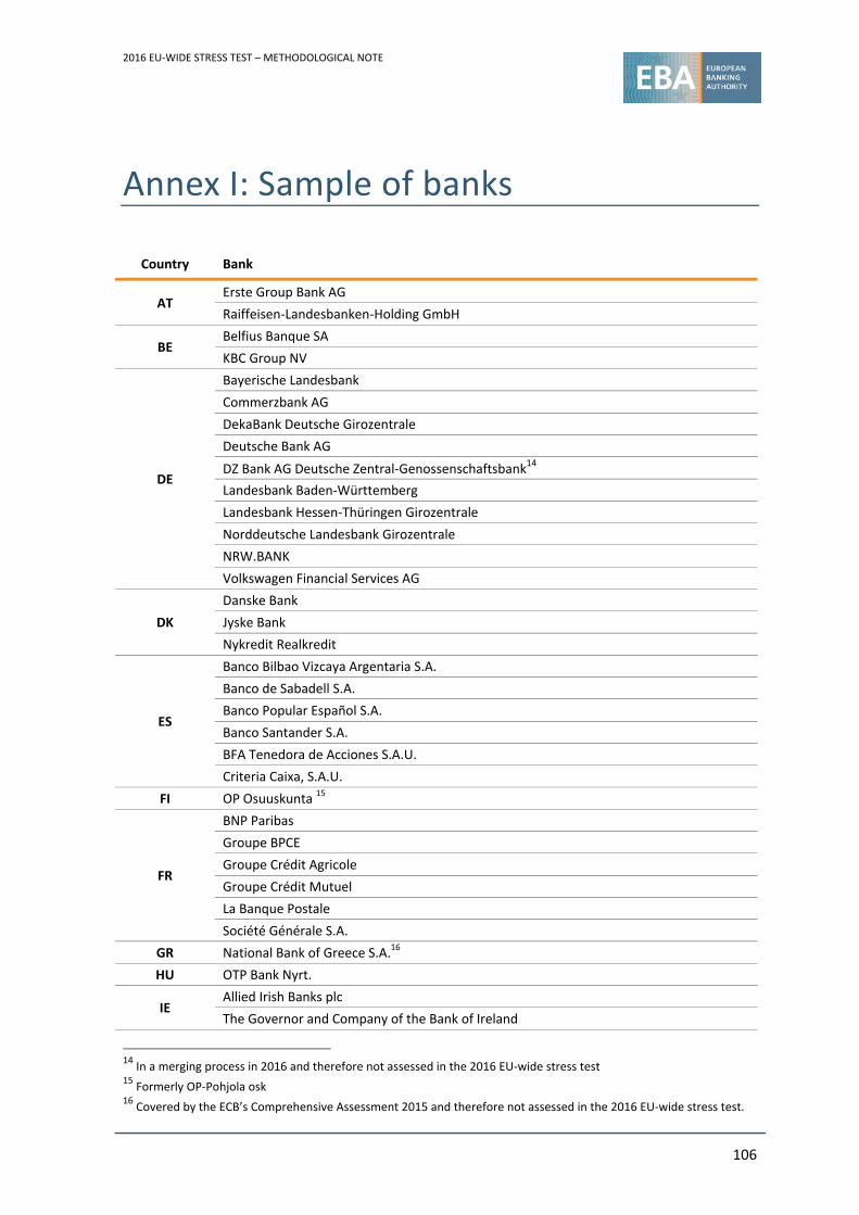
2016 EU‐WIDE STRESS TEST – METHODOLOGICAL NOTE
106
Annex I: Sample of banks
Country Bank
AT Erste Group Bank AG
Raiffeisen‐Landesbanken‐Holding GmbH
BE Belfius Banque SA
KBC Group NV
DE
Bayerische Landesbank
Commerzbank AG
DekaBank Deutsche Girozentrale
Deutsche Bank AG
DZ Bank AG Deutsche Zentral‐Genossenschaftsbank14
Landesbank Baden‐Württemberg
Landesbank Hessen‐Thüringen Girozentrale
Norddeutsche Landesbank Girozentrale
NRW.BANK
Volkswagen Financial Services AG
DK
Danske Bank
Jyske Bank
Nykredit Realkredit
ES
Banco Bilbao Vizcaya Argentaria S.A.
Banco de Sabadell S.A.
Banco Popular Español S.A.
Banco Santander S.A.
BFA Tenedora de Acciones S.A.U.
Criteria Caixa, S.A.U.
FI OP Osuuskunta 15
FR
BNP Paribas
Groupe BPCE
Groupe Crédit Agricole
Groupe Crédit Mutuel
La Banque Postale
Société Générale S.A.
GR National Bank of Greece S.A.16
HU OTP Bank Nyrt.
IE Allied Irish Banks plc
The Governor and Company of the Bank of Ireland
14 In a merging process in 2016 and therefore not assessed in the 2016 EU‐wide stress test
15 Formerly OP‐Pohjola osk
16 Covered by the ECB’s Comprehensive Assessment 2015 and therefore not assessed in the 2016 EU‐wide stress test.
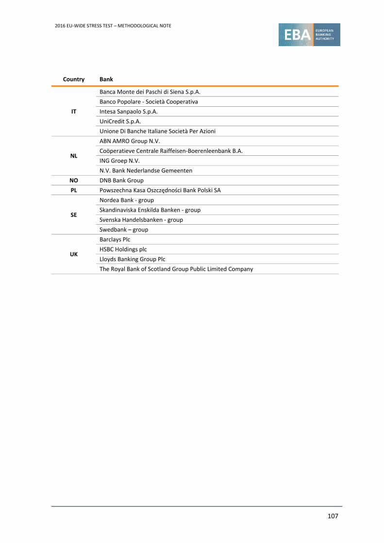
2016 EU‐WIDE STRESS TEST – METHODOLOGICAL NOTE
107
Country Bank
IT
Banca Monte dei Paschi di Siena S.p.A.
Banco Popolare ‐ Società Cooperativa
Intesa Sanpaolo S.p.A.
UniCredit S.p.A.
Unione Di Banche Italiane Società Per Azioni
NL
ABN AMRO Group N.V.
Coöperatieve Centrale Raiffeisen‐Boerenleenbank B.A.
ING Groep N.V.
N.V. Bank Nederlandse Gemeenten
NO DNB Bank Group
PL Powszechna Kasa Oszczędności Bank Polski SA
SE
Nordea Bank ‐ group
Skandinaviska Enskilda Banken ‐ group
Svenska Handelsbanken ‐ group
Swedbank – group
UK
Barclays Plc
HSBC Holdings plc
Lloyds Banking Group Plc
The Royal Bank of Scotland Group Public Limited Company
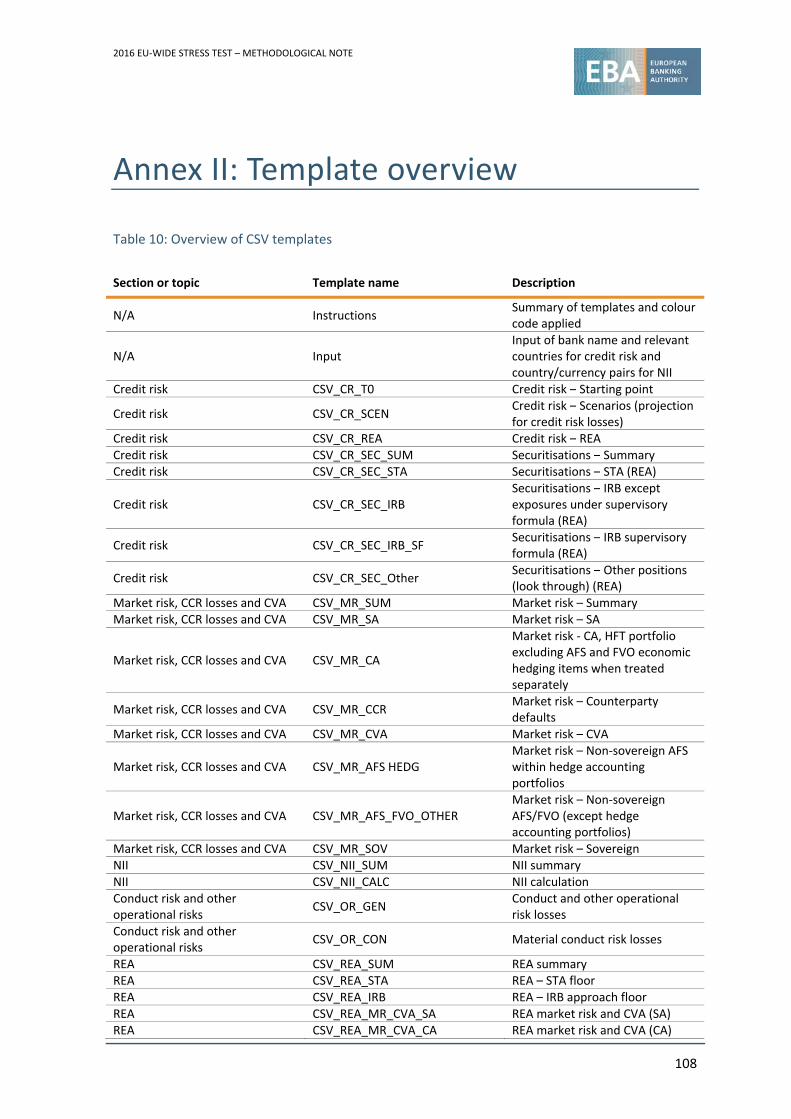
2016 EU‐WIDE STRESS TEST – METHODOLOGICAL NOTE
108
Annex II: Template overview
Table 10: Overview of CSV templates
Section or topic Template name Description
N/A Instructions Summary of templates and colour code applied
N/A Input Input of bank name and relevant countries for credit risk and country/currency pairs for NII
Credit risk CSV_CR_T0 Credit risk – Starting point
Credit risk CSV_CR_SCEN Credit risk – Scenarios (projection for credit risk losses)
Credit risk CSV_CR_REA Credit risk – REA Credit risk CSV_CR_SEC_SUM Securitisations – SummaryCredit risk CSV_CR_SEC_STA Securitisations – STA (REA)
Credit risk CSV_CR_SEC_IRB Securitisations – IRB except exposures under supervisory formula (REA)
Credit risk CSV_CR_SEC_IRB_SF Securitisations – IRB supervisory formula (REA)
Credit risk CSV_CR_SEC_Other Securitisations – Other positions (look through) (REA)
Market risk, CCR losses and CVA CSV_MR_SUM Market risk – Summary Market risk, CCR losses and CVA CSV_MR_SA Market risk – SA
Market risk, CCR losses and CVA CSV_MR_CA
Market risk ‐ CA, HFT portfolio excluding AFS and FVO economic hedging items when treated separately
Market risk, CCR losses and CVA CSV_MR_CCR Market risk – Counterparty defaults
Market risk, CCR losses and CVA CSV_MR_CVA Market risk – CVA
Market risk, CCR losses and CVA CSV_MR_AFS HEDG Market risk – Non‐sovereign AFS within hedge accounting portfolios
Market risk, CCR losses and CVA CSV_MR_AFS_FVO_OTHER Market risk – Non‐sovereign AFS/FVO (except hedge accounting portfolios)
Market risk, CCR losses and CVA CSV_MR_SOV Market risk – Sovereign NII CSV_NII_SUM NII summary NII CSV_NII_CALC NII calculation Conduct risk and other operational risks
CSV_OR_GEN Conduct and other operational risk losses
Conduct risk and other operational risks
CSV_OR_CON Material conduct risk losses
REA CSV_REA_SUM REA summary REA CSV_REA_STA REA – STA floor REA CSV_REA_IRB REA – IRB approach floor REA CSV_REA_MR_CVA_SA REA market risk and CVA (SA)REA CSV_REA_MR_CVA_CA REA market risk and CVA (CA)
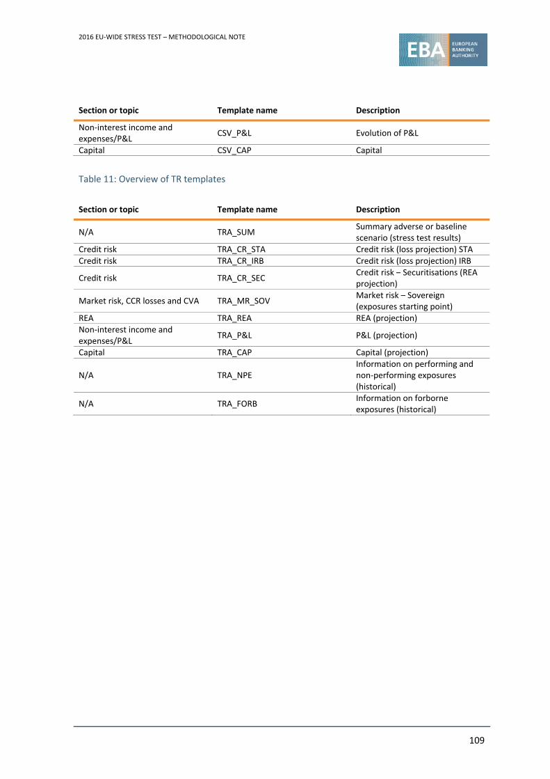
2016 EU‐WIDE STRESS TEST – METHODOLOGICAL NOTE
109
Section or topic Template name Description
Non‐interest income and expenses/P&L
CSV_P&L Evolution of P&L
Capital CSV_CAP Capital
Table 11: Overview of TR templates
Section or topic Template name Description
N/A TRA_SUM Summary adverse or baseline scenario (stress test results)
Credit risk TRA_CR_STA Credit risk (loss projection) STACredit risk TRA_CR_IRB Credit risk (loss projection) IRB
Credit risk TRA_CR_SEC Credit risk – Securitisations (REAprojection)
Market risk, CCR losses and CVA TRA_MR_SOV Market risk – Sovereign (exposures starting point)
REA TRA_REA REA (projection) Non‐interest income and expenses/P&L
TRA_P&L P&L (projection)
Capital TRA_CAP Capital (projection)
N/A TRA_NPE Information on performing and non‐performing exposures (historical)
N/A TRA_FORB Information on forborne exposures (historical)
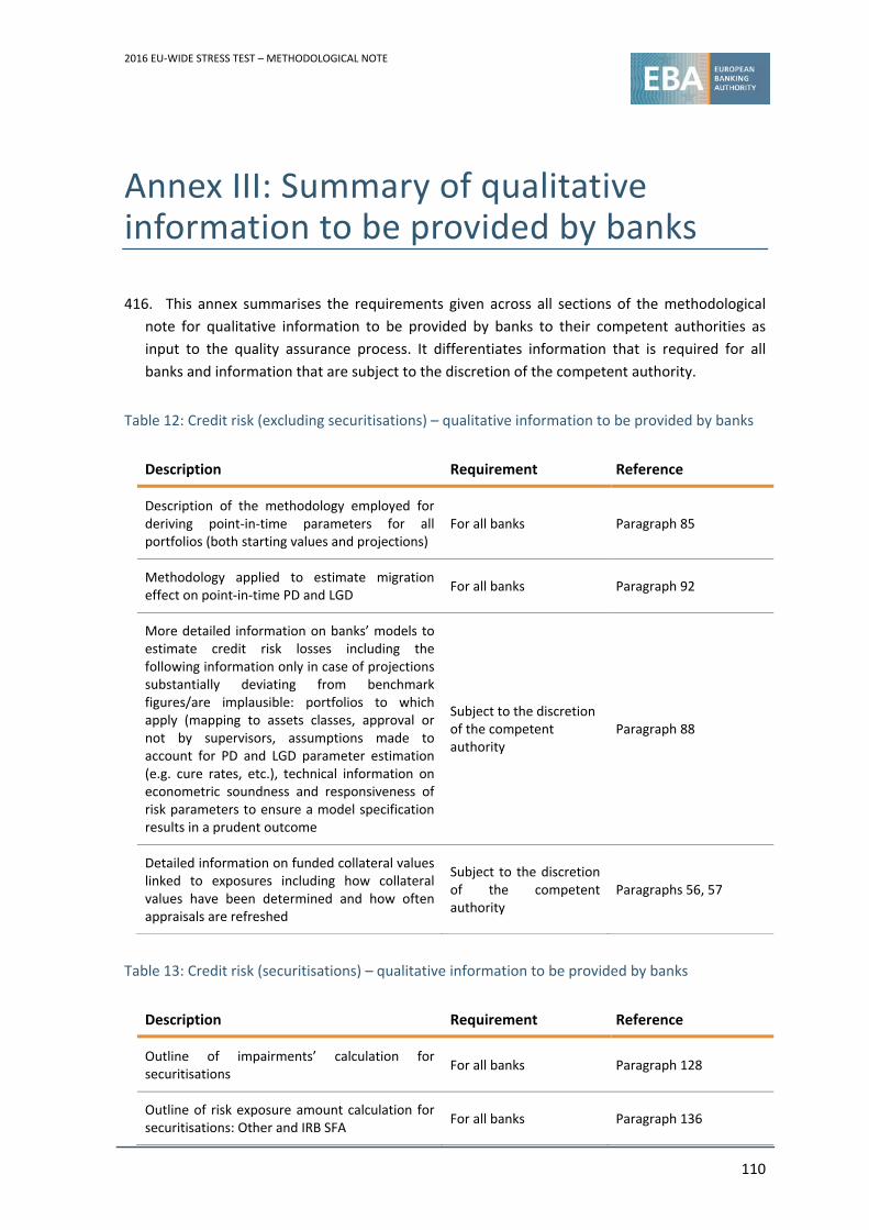
2016 EU‐WIDE STRESS TEST – METHODOLOGICAL NOTE
110
Annex III: Summary of qualitative information to be provided by banks
416. This annex summarises the requirements given across all sections of the methodological
note for qualitative information to be provided by banks to their competent authorities as
input to the quality assurance process. It differentiates information that is required for all
banks and information that are subject to the discretion of the competent authority.
Table 12: Credit risk (excluding securitisations) – qualitative information to be provided by banks
Description Requirement Reference
Description of the methodology employed for deriving point‐in‐time parameters for all portfolios (both starting values and projections)
For all banks Paragraph 85
Methodology applied to estimate migration effect on point‐in‐time PD and LGD
For all banks Paragraph 92
More detailed information on banks’ models to estimate credit risk losses including the following information only in case of projections substantially deviating from benchmark figures/are implausible: portfolios to which apply (mapping to assets classes, approval or not by supervisors, assumptions made to account for PD and LGD parameter estimation (e.g. cure rates, etc.), technical information on econometric soundness and responsiveness of risk parameters to ensure a model specification results in a prudent outcome
Subject to the discretion of the competent authority
Paragraph 88
Detailed information on funded collateral values linked to exposures including how collateral values have been determined and how often appraisals are refreshed
Subject to the discretion of the competent authority
Paragraphs 56, 57
Table 13: Credit risk (securitisations) – qualitative information to be provided by banks
Description Requirement Reference
Outline of impairments’ calculation for securitisations
For all banks Paragraph 128
Outline of risk exposure amount calculation for securitisations: Other and IRB SFA
For all banks Paragraph 136
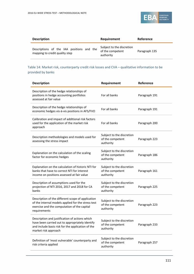
2016 EU‐WIDE STRESS TEST – METHODOLOGICAL NOTE
111
Description Requirement Reference
Descriptions of the IAA positions and the mapping to credit quality step
Subject to the discretion of the competent authority
Paragraph 135
Table 14: Market risk, counterparty credit risk losses and CVA – qualitative information to be
provided by banks
Description Requirement Reference
Description of the hedge relationships of positions in hedge accounting portfolios assessed at fair value
For all banks Paragraph 191
Description of the hedge relationships of economic hedges vis‐à‐vis positions in AFS/FVO
For all banks Paragraph 191
Calibration and impact of additional risk factors used for the application of the market risk approach
For all banks Paragraph 200
Description methodologies and models used for assessing the stress impact
Subject to the discretion of the competent authority
Paragraph 223
Explanation on the calculation of the scaling factor for economic hedges
Subject to the discretion of the competent authority
Paragraph 186
Explanation on the calculation of historic NTI for banks that have to correct NTI for interest income on positions assessed at fair value
Subject to the discretion of the competent authority
Paragraph 161
Description of assumptions used for the projection of NTI 2016, 2017 and 2018 for CA banks
Subject to the discretion of the competent authority
Paragraph 225
Description of the different scope of application of the internal models applied for the stress test exercise and the computation of the capital requirements
Subject to the discretion of the competent authority
Paragraph 223
Description and justification of actions which have been carried out to appropriately identify and include basis risk for the application of the market risk approach
Subject to the discretion of the competent authority
Paragraph 233
Definition of ‘most vulnerable’ counterparty and risk criteria applied
Subject to the discretion of the competent authority
Paragraph 257
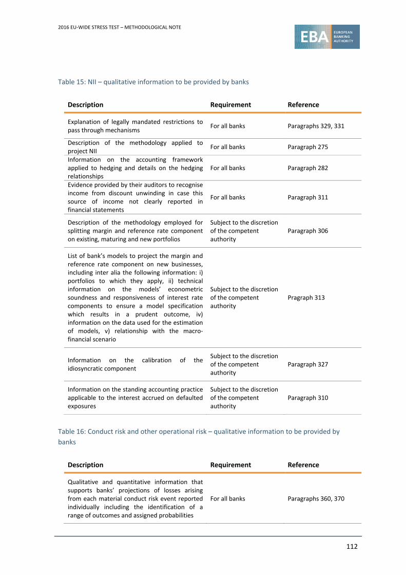
2016 EU‐WIDE STRESS TEST – METHODOLOGICAL NOTE
112
Table 15: NII – qualitative information to be provided by banks
Description Requirement Reference
Explanation of legally mandated restrictions to pass through mechanisms
For all banks Paragraphs 329, 331
Description of the methodology applied to project NII
For all banks Paragraph 275
Information on the accounting framework applied to hedging and details on the hedging relationships
For all banks Paragraph 282
Evidence provided by their auditors to recognise income from discount unwinding in case this source of income not clearly reported in financial statements
For all banks Paragraph 311
Description of the methodology employed for splitting margin and reference rate component on existing, maturing and new portfolios
Subject to the discretion of the competent authority
Paragraph 306
List of bank’s models to project the margin and reference rate component on new businesses, including inter alia the following information: i) portfolios to which they apply, ii) technical information on the models’ econometric soundness and responsiveness of interest rate components to ensure a model specification which results in a prudent outcome, iv) information on the data used for the estimation of models, v) relationship with the macro‐financial scenario
Subject to the discretion of the competent authority
Pragraph 313
Information on the calibration of the idiosyncratic component
Subject to the discretion of the competent authority
Paragraph 327
Information on the standing accounting practice applicable to the interest accrued on defaulted exposures
Subject to the discretion of the competent authority
Paragraph 310
Table 16: Conduct risk and other operational risk – qualitative information to be provided by
banks
Description Requirement Reference
Qualitative and quantitative information that supports banks’ projections of losses arising from each material conduct risk event reported individually including the identification of a range of outcomes and assigned probabilities
For all banks Paragraphs 360, 370
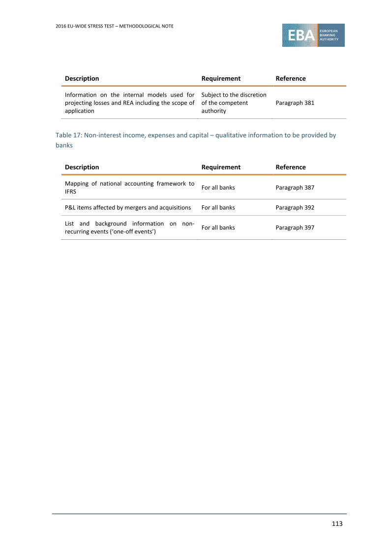
2016 EU‐WIDE STRESS TEST – METHODOLOGICAL NOTE
113
Description Requirement Reference
Information on the internal models used for projecting losses and REA including the scope of application
Subject to the discretion of the competent authority
Paragraph 381
Table 17: Non‐interest income, expenses and capital – qualitative information to be provided by
banks
Description Requirement Reference
Mapping of national accounting framework to IFRS
For all banks Paragraph 387
P&L items affected by mergers and acquisitions For all banks Paragraph 392
List and background information on non‐recurring events (‘one‐off events’)
For all banks Paragraph 397
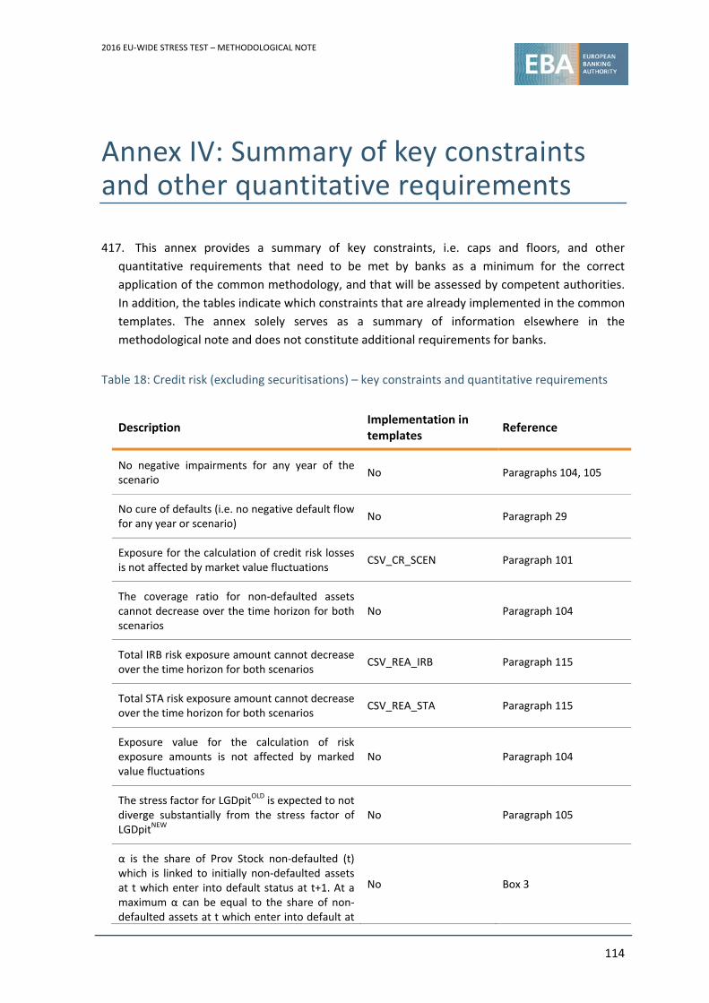
2016 EU‐WIDE STRESS TEST – METHODOLOGICAL NOTE
114
Annex IV: Summary of key constraints and other quantitative requirements
417. This annex provides a summary of key constraints, i.e. caps and floors, and other
quantitative requirements that need to be met by banks as a minimum for the correct
application of the common methodology, and that will be assessed by competent authorities.
In addition, the tables indicate which constraints that are already implemented in the common
templates. The annex solely serves as a summary of information elsewhere in the
methodological note and does not constitute additional requirements for banks.
Table 18: Credit risk (excluding securitisations) – key constraints and quantitative requirements
Description Implementation in templates
Reference
No negative impairments for any year of the scenario
No Paragraphs 104, 105
No cure of defaults (i.e. no negative default flow for any year or scenario)
No Paragraph 29
Exposure for the calculation of credit risk losses is not affected by market value fluctuations
CSV_CR_SCEN Paragraph 101
The coverage ratio for non‐defaulted assets cannot decrease over the time horizon for both scenarios
No Paragraph 104
Total IRB risk exposure amount cannot decrease over the time horizon for both scenarios
CSV_REA_IRB Paragraph 115
Total STA risk exposure amount cannot decrease over the time horizon for both scenarios
CSV_REA_STA Paragraph 115
Exposure value for the calculation of risk exposure amounts is not affected by marked value fluctuations
No Paragraph 104
The stress factor for LGDpitOLD is expected to not diverge substantially from the stress factor of LGDpitNEW
No Paragraph 105
α is the share of Prov Stock non‐defaulted (t) which is linked to initially non‐defaulted assets at t which enter into default status at t+1. At a maximum α can be equal to the share of non‐defaulted assets at t which enter into default at
No Box 3
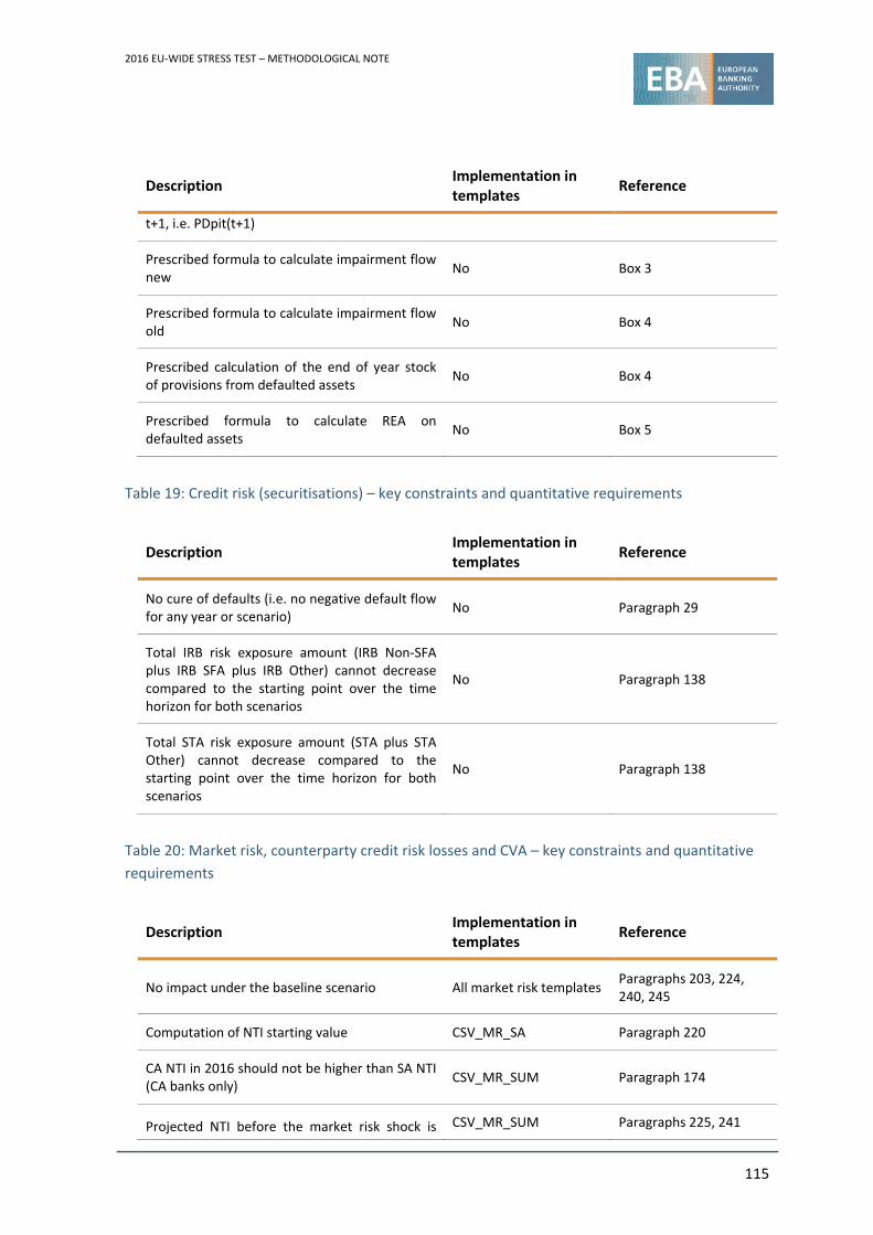
2016 EU‐WIDE STRESS TEST – METHODOLOGICAL NOTE
115
Description Implementation in templates
Reference
t+1, i.e. PDpit(t+1)
Prescribed formula to calculate impairment flow new
No Box 3
Prescribed formula to calculate impairment flow old
No Box 4
Prescribed calculation of the end of year stock of provisions from defaulted assets
No Box 4
Prescribed formula to calculate REA on defaulted assets
No Box 5
Table 19: Credit risk (securitisations) – key constraints and quantitative requirements
Description Implementation in templates
Reference
No cure of defaults (i.e. no negative default flow for any year or scenario)
No Paragraph 29
Total IRB risk exposure amount (IRB Non‐SFA plus IRB SFA plus IRB Other) cannot decrease compared to the starting point over the time horizon for both scenarios
No Paragraph 138
Total STA risk exposure amount (STA plus STA Other) cannot decrease compared to the starting point over the time horizon for both scenarios
No Paragraph 138
Table 20: Market risk, counterparty credit risk losses and CVA – key constraints and quantitative
requirements
Description Implementation in templates
Reference
No impact under the baseline scenario All market risk templates Paragraphs 203, 224, 240, 245
Computation of NTI starting value CSV_MR_SA Paragraph 220
CA NTI in 2016 should not be higher than SA NTI (CA banks only)
CSV_MR_SUM Paragraph 174
Projected NTI before the market risk shock is CSV_MR_SUM Paragraphs 225, 241
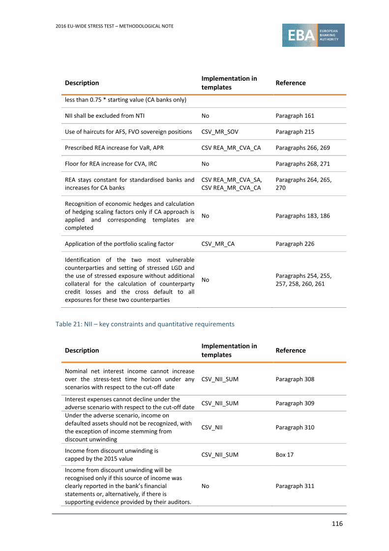
2016 EU‐WIDE STRESS TEST – METHODOLOGICAL NOTE
116
Description Implementation in templates
Reference
less than 0.75 * starting value (CA banks only)
NII shall be excluded from NTI No Paragraph 161
Use of haircuts for AFS, FVO sovereign positions CSV_MR_SOV Paragraph 215
Prescribed REA increase for VaR, APR CSV REA_MR_CVA_CA Paragraphs 266, 269
Floor for REA increase for CVA, IRC No Paragraphs 268, 271
REA stays constant for standardised banks and increases for CA banks
CSV REA_MR_CVA_SA, CSV REA_MR_CVA_CA
Paragraphs 264, 265, 270
Recognition of economic hedges and calculation of hedging scaling factors only if CA approach is applied and corresponding templates are completed
No Paragraphs 183, 186
Application of the portfolio scaling factor CSV_MR_CA Paragraph 226
Identification of the two most vulnerable counterparties and setting of stressed LGD and the use of stressed exposure without additional collateral for the calculation of counterparty credit losses and the cross default to all exposures for these two counterparties
No Paragraphs 254, 255, 257, 258, 260, 261
Table 21: NII – key constraints and quantitative requirements
Description Implementation in templates
Reference
Nominal net interest income cannot increase over the stress‐test time horizon under any scenarios with respect to the cut‐off date
CSV_NII_SUM Paragraph 308
Interest expenses cannot decline under the adverse scenario with respect to the cut‐off date
CSV_NII_SUM Paragraph 309
Under the adverse scenario, income on defaulted assets should not be recognized, with the exception of income stemming from discount unwinding
CSV_NII Paragraph 310
Income from discount unwinding is capped by the 2015 value
CSV_NII_SUM Box 17
Income from discount unwinding will be recognised only if this source of income was clearly reported in the bank’s financial statements or, alternatively, if there is supporting evidence provided by their auditors.
No Paragraph 311
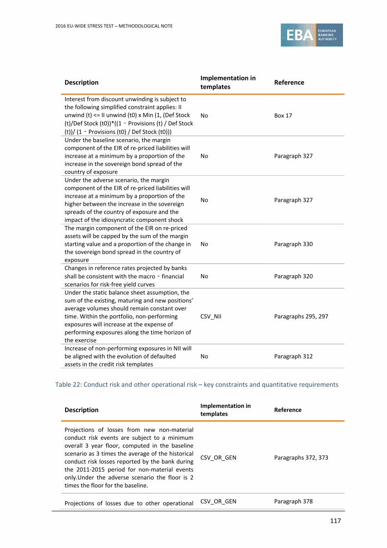
2016 EU‐WIDE STRESS TEST – METHODOLOGICAL NOTE
117
Description Implementation in templates
Reference
Interest from discount unwinding is subject to the following simplified constraint applies: II unwind (t) <= II unwind (t0) x Min (1, (Def Stock
(t)/Def Stock (t0))*((1‐Provisions (t) / Def Stock
(t))/ (1‐Provisions (t0) / Def Stock (t0)))
No Box 17
Under the baseline scenario, the margin component of the EIR of re‐priced liabilities will increase at a minimum by a proportion of the increase in the sovereign bond spread of the country of exposure
No Paragraph 327
Under the adverse scenario, the margin component of the EIR of re‐priced liabilities will increase at a minimum by a proportion of the higher between the increase in the sovereign spreads of the country of exposure and the impact of the idiosyncratic component shock
No Paragraph 327
The margin component of the EIR on re‐priced assets will be capped by the sum of the margin starting value and a proportion of the change in the sovereign bond spread in the country of exposure
No Paragraph 330
Changes in reference rates projected by banks
shall be consistent with the macro‐financial scenarios for risk‐free yield curves
No Paragraph 320
Under the static balance sheet assumption, the sum of the existing, maturing and new positions’ average volumes should remain constant over time. Within the portfolio, non‐performing exposures will increase at the expense of performing exposures along the time horizon of the exercise
CSV_NII Paragraphs 295, 297
Increase of non‐performing exposures in NII will be aligned with the evolution of defaulted assets in the credit risk templates
No Paragraph 312
Table 22: Conduct risk and other operational risk – key constraints and quantitative requirements
Description Implementation in templates
Reference
Projections of losses from new non‐material conduct risk events are subject to a minimum overall 3 year floor, computed in the baseline scenario as 3 times the average of the historical conduct risk losses reported by the bank during the 2011‐2015 period for non‐material events only.Under the adverse scenario the floor is 2 times the floor for the baseline.
CSV_OR_GEN Paragraphs 372, 373
Projections of losses due to other operational CSV_OR_GEN Paragraph 378
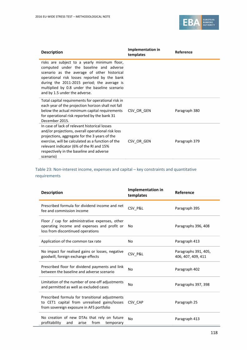
2016 EU‐WIDE STRESS TEST – METHODOLOGICAL NOTE
118
Description Implementation in templates
Reference
risks are subject to a yearly minimum floor, computed under the baseline and adverse scenario as the average of other historical operational risk losses reported by the bank during the 2011‐2015 period; the average is multiplied by 0.8 under the baseline scenario and by 1.5 under the adverse.
Total capital requirements for operational risk in each year of the projection horizon shall not fall below the actual minimum capital requirements for operational risk reported by the bank 31 December 2015.
CSV_OR_GEN Paragraph 380
In case of lack of relevant historical losses and/or projections, overall operational risk loss projections, aggregate for the 3 years of the exercise, will be calculated as a function of the relevant indicator (6% of the RI and 15% respectively in the baseline and adverse scenario)
CSV_OR_GEN Paragraph 379
Table 23: Non‐interest income, expenses and capital – key constraints and quantitative
requirements
Description Implementation in templates
Reference
Prescribed formula for dividend income and net fee and commission income
CSV_P&L Paragraph 395
Floor / cap for administrative expenses, other operating income and expenses and profit or loss from discontinued operations
No Paragraphs 396, 408
Application of the common tax rate No Paragraph 413
No impact for realised gains or losses, negative goodwill, foreign exchange effects
CSV_P&L Paragraphs 391, 405, 406, 407, 409, 411
Prescribed floor for dividend payments and link between the baseline and adverse scenario
No Paragraph 402
Limitation of the number of one‐off adjustments and permitted as well as excluded cases
No Paragraphs 397, 398
Prescribed formula for transitional adjustments to CET1 capital from unrealised gains/losses from sovereign exposure in AFS portfolio
CSV_CAP Paragraph 25
No creation of new DTAs that rely on future profitability and arise from temporary
No Paragraph 413

2016 EU‐WIDE STRESS TEST – METHODOLOGICAL NOTE
119
Description Implementation in templates
Reference
differences
The creation of DTAs that rely on future profitability and do not arise from temporary differences is limited to the offsetting of negative pre‐tax profits
No Paragraph 413