© 2014 Mohith Manjunath

WAVE TAILORING GRANULAR MATERIALS: EFFECT OF RANDOMNESSAND PLANE WAVE PROPAGATION

BY

MOHITH MANJUNATH

DISSERTATION

Submitted in partial fulfillment of the requirementsfor the degree of Doctor of Philosophy in Aerospace Engineering

in the Graduate College of theUniversity of Illinois at Urbana-Champaign, 2014

Urbana, Illinois

Doctoral Committee:

Professor Philippe H. Geubelle, ChairProfessor John LambrosProfessor Alexander VakakisAssistant Professor Oscar Lopez-PamiesAssistant Professor Huck Beng Chew

Abstract

This thesis addresses some of the fundamental issues/aspects as well as practical

significance of impact response in granular media. In the first part of the study, we

investigate numerically the effect of randomness in material and geometric proper-

ties on wave propagation behavior in 1D and 2D granular media. Results obtained

for both 1D chains and 2D media show the kinetic energy amplitude decays with

distance, with the rate of decay found to depend on the level of randomness and

the distance from point of impact. The kinetic energy amplitude initially decays

exponentially before transitioning to a universal power-law regime that is valid for

all levels of randomness. The power-law regime is fundamentally due to the pres-

ence of secondary waves whose amplitude is higher than that of the primary wave

after the point of transition. Another key result quantifies the rate of decay of force

amplitude in a 2D square packing system along various directions of propagation.

Several contour maps are obtained that demonstrate the directions along which we

can obtain minimum or maximum decay, which are practically relevant for material

design.

In the second part of the study, we focus on plane wave propagation in higher

dimensional structures. In the case of 2D and 3D monodisperse granular media,

we demonstrate an equivalence with 1D chains and consequently derive the rela-

tion between wavefront speed and force amplitude in higher dimensional systems.

Subsequent normalization results in a universal wavefront speed-force amplitude

relation that is valid across the different ordered 2D and 3D systems such as hexag-

ii

onal, body-centered cubic and face-centered cubic packings. We also investigate the

effect of angular impact on granular media and discuss mechanism through which

the shearing component of the loading is propagated in the system. In the case of

2D dimer systems, we consider a square packing system with interstitial intruders.

Following the procedure that we developed for monodisperse granular media, we

obtain an equivalent nonlocal dimer chain that gives the same response with rele-

vant scaling of material properties. In this study, we demonstrate the existence of

a new family of plane solitary waves over a wide range of material and geometric

properties. We also indicate a discrete set of solutions for which there is locally

maximum decay, thereby showing promise for wave mitigation as well.

In the last part of our study, we conduct a preliminary study to investigate the

vibration response of beams made of a granular chain embedded in a linear elastic

matrix. A nonlinear, dynamic finite element model is developed, in which the gran-

ular chain is converted to a series of 1D nonlinear bar elements whose contribution is

added to linear quadrilateral elements. We study the bending response by applying

a harmonic loading on a composite beam fixed on both ends and show a funda-

mental difference between the dynamic response of a linear elastic beam and the

embedded granular system at resonance. Unlike a linear elastic beam, we find the

deflection of an embedded granular system to be finite at resonance. Furthermore,

in the presence of precompression, the frequency at which the composite beam de-

flection is maximum can be controlled based on the level of precompression, acting

as an active control feature in material design.

iii

To my teacher.

iv

Acknowledgments

Firstly, I am very thankful to my advisor Prof. Philippe Geubelle for his guidance

all through my years at the University of Illinois. In spite of his administrative

responsibilities, he made sure to take some time off every week to meet his students

and thus making our progress smooth. I also take the opportunity to thank my

lab mates: Ahmad Najafi, Amnaya Awasthi, Mahesh Manchakattil Sucheendran,

Masoud Safdari, Erheng Wang and Raj Kumar Pal, to name a few, for helpful

discussions and more importantly giving an opportunity to contemplate about life

in general. I really appreciate Professors John Lambros, Alexander Vakakis, Oscar

Lopez-Pamies and Huck Beng Chew for serving as my committee members and

giving suggestions over the course of my doctoral study.

I am really grateful to my teacher and a wonderful set of friends here in Urbana,

in whose association I am learning to see the world with a different attitude. I owe

special thanks to my parents and grandmother for playing their roles in bringing

me up and supporting me in my decisions.

v

Table of Contents

Chapter 1 Introduction . . . . . . . . . . . . . . . . . . . . . . . . . . . . . . . 11.1 Literature Review . . . . . . . . . . . . . . . . . . . . . . . . . . . . . . 41.2 Thesis Objectives and Outline . . . . . . . . . . . . . . . . . . . . . . . 13

Chapter 2 Randomness in 1D granular chains . . . . . . . . . . . . . . . . . 182.1 Problem description and numerical setup . . . . . . . . . . . . . . . . 192.2 Randomness in mass . . . . . . . . . . . . . . . . . . . . . . . . . . . . 21

2.2.1 Decay in force amplitude . . . . . . . . . . . . . . . . . . . . . 252.2.2 Decay of the maximum kinetic energy . . . . . . . . . . . . . . 272.2.3 Normalization of response over different impact velocities and

Young’s moduli . . . . . . . . . . . . . . . . . . . . . . . . . . . 302.2.4 Evolution of the force amplitude . . . . . . . . . . . . . . . . . 332.2.5 Distribution of energy during wave propagation . . . . . . . . 36

2.3 Randomness in Young’s modulus and radius . . . . . . . . . . . . . . 412.4 Conclusions . . . . . . . . . . . . . . . . . . . . . . . . . . . . . . . . . 44

Chapter 3 Randomness in 2D granular media . . . . . . . . . . . . . . . . . 463.1 Problem definition . . . . . . . . . . . . . . . . . . . . . . . . . . . . . 473.2 Results and discussion . . . . . . . . . . . . . . . . . . . . . . . . . . . 51

3.2.1 Characteristics of wave propagation . . . . . . . . . . . . . . . 513.2.2 Force amplitude decay . . . . . . . . . . . . . . . . . . . . . . . 533.2.3 Spatial distribution of peak compressive force . . . . . . . . . 603.2.4 Evolution of ensemble kinetic energy . . . . . . . . . . . . . . 67

3.3 Conclusions . . . . . . . . . . . . . . . . . . . . . . . . . . . . . . . . . 69

Chapter 4 Plane wave propagation in monodisperse granular media . . . 714.1 Numerical setup . . . . . . . . . . . . . . . . . . . . . . . . . . . . . . . 734.2 Normal impact . . . . . . . . . . . . . . . . . . . . . . . . . . . . . . . 75

4.2.1 Analytical study . . . . . . . . . . . . . . . . . . . . . . . . . . 754.2.2 Verification . . . . . . . . . . . . . . . . . . . . . . . . . . . . . 784.2.3 Normalization . . . . . . . . . . . . . . . . . . . . . . . . . . . . 79

4.3 Angular impact: 2D hexagonal packing . . . . . . . . . . . . . . . . . 804.3.1 Numerical observations . . . . . . . . . . . . . . . . . . . . . . 814.3.2 Analytical predictions . . . . . . . . . . . . . . . . . . . . . . . 86

4.4 Conclusions . . . . . . . . . . . . . . . . . . . . . . . . . . . . . . . . . 97

vi

Chapter 5 Plane wave propagation in dimer granular media . . . . . . . . 995.1 Problem statement . . . . . . . . . . . . . . . . . . . . . . . . . . . . . 1015.2 Numerical Results . . . . . . . . . . . . . . . . . . . . . . . . . . . . . . 102

5.2.1 Equivalent 1D system . . . . . . . . . . . . . . . . . . . . . . . 1025.2.2 Numerical observations . . . . . . . . . . . . . . . . . . . . . . 1055.2.3 Extraction of solitary waves . . . . . . . . . . . . . . . . . . . . 107

5.3 Analytical investigation . . . . . . . . . . . . . . . . . . . . . . . . . . 1155.3.1 Quasi-continuum approximation . . . . . . . . . . . . . . . . . 1155.3.2 Asymptotic analysis . . . . . . . . . . . . . . . . . . . . . . . . 122

5.4 Conclusions . . . . . . . . . . . . . . . . . . . . . . . . . . . . . . . . . 130

Chapter 6 Embedded granular systems . . . . . . . . . . . . . . . . . . . . . 1326.1 Problem description and numerical setup . . . . . . . . . . . . . . . . 1336.2 Finite element formulation . . . . . . . . . . . . . . . . . . . . . . . . . 1356.3 Implementation . . . . . . . . . . . . . . . . . . . . . . . . . . . . . . . 1376.4 Dynamic code verification . . . . . . . . . . . . . . . . . . . . . . . . . 1386.5 Convergence studies . . . . . . . . . . . . . . . . . . . . . . . . . . . . 1406.6 Results: dynamic loading . . . . . . . . . . . . . . . . . . . . . . . . . 143

6.6.1 Linear elastic beam . . . . . . . . . . . . . . . . . . . . . . . . . 1436.6.2 Embedded granular system . . . . . . . . . . . . . . . . . . . . 145

6.7 Conclusions . . . . . . . . . . . . . . . . . . . . . . . . . . . . . . . . . 151

Chapter 7 Conclusions and Future Work . . . . . . . . . . . . . . . . . . . . 1537.1 Key contributions . . . . . . . . . . . . . . . . . . . . . . . . . . . . . . 1537.2 Future directions . . . . . . . . . . . . . . . . . . . . . . . . . . . . . . 155

Appendix A Finite element formulation . . . . . . . . . . . . . . . . . . . . 160A.1 Force-displacement relations . . . . . . . . . . . . . . . . . . . . . . . 160A.2 Tangent stiffness matrix . . . . . . . . . . . . . . . . . . . . . . . . . . 161A.3 Newmark method . . . . . . . . . . . . . . . . . . . . . . . . . . . . . . 162

References . . . . . . . . . . . . . . . . . . . . . . . . . . . . . . . . . . . . . . . 164

vii

Chapter 1

Introduction

Granular media are a unique class of materials whose behavior is different from

the three well-known states of matter: solids, liquids and gases. Granular media

possess some characteristics of each of the three phases: they can be packed just

like solids when the grains are relatively stationary and they can also be made to

take the shape of their container like liquids; also, when a container of granular

media is vigorously shaken, the grains disperse with infrequent collisions, similar

to a gas. Granular materials are discrete particles whose sizes can vary anywhere

from a few microns to several kilometers. Among the various granular materials,

colloidal particles are typically less than a micron in size, clay particle’s size is about

few microns, sand particles are usually order of few hundred microns, granule or

gravel have characteristic dimension of order of few millimeters and boulders are

very large particles with size ranging from tens of centimeters to several kilometers.

Each of the above mentioned classes of granular materials is a research area in itself.

Of the many examples found in nature, sand is one case of a very simple form of

granular medium commonly encountered. Yet the understanding of the response of

sand remains elusive due to its complexity. A key characteristic subject of multiple

studies is the angle of repose, which is defined as the angle between a sandpile

and the horizontal [1]. Beyond a certain angle of repose, the sandpile forms an

avalanche which can build in size very quickly as it flows down the slope. Granular

materials of various shapes and sizes are also employed in a wide range of industrial

applications. Agricultural enterprises need to store, pack and transport food items

1

such as rice and nuts which are granular in nature. Similarly, the pharmaceutical

industry requires different ways to optimally store the powders and manufacture

various medicines. Mining is another example where coal, a granular material, is

stored and transported often to various industries.

Most of the above examples utilize granular materials usually of the size of

few microns to few hundred microns. One of the primary goals of our study is

to design a new class of materials that would possess features such as stress wave

mitigation, energy conservation or tailoring upon impact. Therefore, in order to

derive more flexibility in modifying certain properties of the system at the particle

level, we consider granular materials of the size of granules which are spherical in

shape (beads) and a few millimeters in diameter. The spheres are stacked either

next to each other in a line (1D) or closely packed in an ordered manner in 2D

and 3D. In order to take advantage of granular materials for wave mitigation and

tailoring, we need to first understand how energy travels in a granular system.

Impact on a granular material system causes the energy to propagate along the

various inter-particle contacts, which deform due to the relative motion between

the contacting particles. If the stress developed at a contact is less than the yield

stress of the material, the spheres remain elastic; otherwise there will be permanent

plastic deformation.

In granular media with spherical particles, we need an elastic force-displacement

model between two spheres in contact in order to perform numerical simulations or

compare with experiments. Several researchers [2, 3] have found that the classical

Hertz theory for elastic solids in contact provides satisfactory results since it was

first proposed in 1882 [4]. In the Hertzian law, the applied load, F, is related to

the distance of approach of the spheres’ centers, δ, as F ∝ δ3/2. The proportionality

factor is a function of material and geometric properties which will be defined in

the later sections.

2

Wave propagation in granular media made of spherical particles is unique as it

differs from wave propagation in linear elastic continuous media in several ways.

In continuous media, both tensile and compressive waves are linear and travel at

constant speeds dependent on the material properties of the medium. In contrast,

wave propagation in granular media intrinsically depends on the nonlinearity at

inter-particle contacts due to the Hertzian law. There is also a second source of non-

linearity which stems from the fact that the spheres do not exert any force in tension,

unlike continuous media. Over the past few decades, the Hertzian law has been

used by various researchers to study the dynamics of granular media [3]. In a 1D

homogeneous chain of spheres just touching each other without initial compression

at contacts, numerical investigation using the Hertzian law and experiments have

demonstrated the presence of nondispersive waves with compact support known

as solitary waves [5]. These solitary waves were first observed in a water channel

where they were found to be stable and travel very long distances without decay.

Unlike a linear elastic wave, the speed of a solitary wave depends upon its ampli-

tude as a consequence of the Hertzian law. For example, in a system of linear elastic

spherical granules, the speed of a solitary wave (Vs) varies with its force amplitude

(Fm) as Vs ∝ F1/6m [5]. Also, the width of a solitary wave in a spherical particle-system

is determined to be about five particle diameters, but in general it depends upon

the shape of the granule [2].

Since the granular materials can be discretely inhomogeneous, i.e., offer the flex-

ibility of altering the material and geometric properties of each granule, there is

enormous scope to employ the materials in a wide range of areas [6]. Thus there is

also a possibility of tailoring the impact energy in preferential directions by changing

the properties locally. These materials find applications in topics such as impurity

or damage detection in materials [7, 8, 9], generation of high-accuracy focusing

and high-energy acoustic pulses [10], and impulse confinement and disintegration

3

[11, 12]. Also, granular systems in the presence of precompression at some or all the

contacts demonstrate a different kind of dynamics whose continuum approximation

is found to follow the Korteweg-de Vries (KdV) equation. The solitary waves in the

case where the contact deformations are much smaller than the precompression are

more closely related to the KdV equation solution [5]. The presence of precompres-

sion allows sound propagation in the granular system and has been successfully

employed in applications and areas such as acoustic lens (or sound bullet) and band

gaps.

1.1 Literature Review

One of the earliest attempts to numerically understand the effect of nonlinearity in

a dynamical system was undertaken by Fermi, Pasta and Ulam [13]. The chosen

dynamical system was a 1D lattice of masses connected by springs with the nearest

neighbors having weak quadratic or cubic interactions in addition to linear interac-

tions, popularly known as the FPU problem or lattice. The goal of their study was

to determine if there was any equipartition of energy among the various modes of

vibration. While the linear case shows that the string of particles vibrates indefi-

nitely according to the initial mode of excitation with equipartition, the FPU lattice

surprisingly did not show equipartition of energy among all the degrees of freedom.

The energy was mostly carried by a particular mode at a given instant of time. In

the following decades, the FPU problem has been revisited and several theoretical

studies were conducted to explain some of the phenomena including a continuum

approximation of the FPU lattice [14].

While the earlier studies considered quadratic or cubic variations, Nesterenko

[5] formulated the problem of a 1D chain of homogeneous spheres interacting via

the Hertzian potential. Nesterenko first assumed that the relative displacements

4

between the contacting spheres to be much smaller than the precompression level

and showed that the resulting continuum approximation has properties of the KdV

equation mentioned earlier. The opposite case, i.e., the relative displacements being

much larger than the precompression level, also showed the existence of solitary

waves in the continuum approximation where a surprisingly simple solution dif-

ferent from the KdV equation was obtained by taking the solution to be a traveling

wave with a certain phase velocity. Nesterenko then performed numerical simu-

lations to confirm the presence of solitary waves in a 1D granular chain. Lazaridi

et al. [15] conducted the earliest set of experiments where a piston of certain mass

impacted a chain of spheres and a comparison was made with numerical results. A

reasonable agreement was found between the experimental and numerical results,

demonstrating solitary waves for the first time in a granular chain with no linear

interaction component (acoustic speed equal to zero). Later, the concept of “sonic

vacuum” was introduced [16] to indicate the inability of a granular chain in ab-

sence of linear interaction component to allow acoustic disturbances to propagate

in the system. Nesterenko [16] performed a more in-depth theoretical analysis of an

equivalent 1D continuum system with stress-strain relationship σ ∝ ξn and n > 1.

The conditions for which solitary waves exist in such systems and the spatial length

of the waves as a function of n were also derived. Further, several experiments

were also conducted [16, 17] to study the characteristics of a solitary wave at the

interface between two sonic vacua. The mass of the piston impacting the first sonic

vacuum was varied, resulting in a series of waves in some cases and a single pulse

in others. The piston mass plays a role because the contact time with the first sphere

depends on the two masses in contact and a higher loading time will lead to the

decomposition of a single wave into series of waves with decreasing amplitude.

Coste et al. [18] conducted detailed experimental analysis on a 1D chain of

spheres with moderate or zero precompression, and the results were consistent

5

with the theoretical predictions of Nesterenko. Wave velocity and force amplitude

measurements demonstrated and verified the nonlinear dependence for both with

and without static force. Following the comprehensive study by Coste et al., few

studies focused on theoretical analysis of the existence of solitary waves in granular

chains. In the first study, Mackay [19] applied the result of Friesecke et al. [20] to

the Hertzian model and concluded that solitary wave exists if the potential energy

is greater than zero and the precompression force F ≥ 0. While Mackay’s study

focused on the Hertzian model, Ji et al. [21] later extended it to a more general class

of granular chains where the power-law exponent n is taken to be arbitrary, i.e., the

shape of the particles are not necessarily spherical. Following a similar approach

as Mackay’s, Ji et al. proved that the criterion for the existence of solitary waves is

n > 1. Several other experiments have also been conducted on homogeneous [22]

and heterogeneous granular media [23], demonstrating solitary wave propagation

and wave speed characteristics. Since the granular materials are highly tunable

to extract required wave propagation behavior [2], these material systems found

potential applications in many areas such as granular protectors [12], acoustic lens

[10], shock mitigation and absorption [3] and band-gaps [24].

Many studies have also focused on tapered and decorated granular chains, whose

design can lead to a wide variety of energy absorption devices [25, 26, 27, 28]. In ana-

lytical consideration of tapered and decorated granular chains, Harbola et al. [27, 28]

used a binary collision approximation, where the pulse is assumed to propagate via

interaction of two particles at a time. Although the model overpredicted the pulse

amplitude in that study, it was found to capture very well other key characteristics,

such as the pulse speed and the decay rate. The interaction of a solitary wave with

a wall or a material interface [11, 29, 30] and characteristics of wave propagation in

chains with different geometries or mass defect [31, 32] have also been subjects of

interest. Recent efforts have focused on extending the granular contact law to in-

6

clude the effects of plasticity for simulating a wider range of granular materials. Pal

et al. [33] conducted a two-part study wherein an elasto-plastic force-displacement

law between two elastic-perfectly plastic spheres in contact was extracted using

finite element analysis and then used to perform wave propagation studies in 1D

granular chains. In the dynamic study, the force amplitude was found to decrease

as expected but a more detailed analysis showed different regimes of decay such as

exponential and inverse regimes. Several scaling laws were derived to effectively

capture the wave propagation characteristics for a wide range of input forces. Fur-

ther, phenomena such as wave trains and wave merging were revealed that require

a more focused research to understand the effect of plasticity on wave propaga-

tion. Carretero-Gonzalez et al. [34] introduced an additional term in the Hertzian

model to capture dissipative effects arising in the experiments other than friction

and plasticity. The additional term comprises of a dissipative force dependent on

the relative velocities of the spheres which has a prefactor and an exponent as the

two unknown parameters. Several experiments and numerical simulations were

performed and systematically compared to obtain the dissipation coefficients for

three different materials. Interestingly, the exponent was found to be approximately

constant for all the materials while the prefactor was material dependent.

Sokolow et al. [35] reported additional set of results on solitary wave train for-

mation in elastic granular chains. Their results demonstrated the effect of striker

mass on wave propagation where a single solitary wave is formed if the striker mass

is less than or equal to the mass of a sphere in the chain while a series of solitary

waves (wave train) is formed otherwise. The solitary waves’ amplitudes decrease

progressively in the wave train and the decay is found to be approximately exponen-

tial. Later, Job et al. [36] performed further analysis of homogeneous and stepped

(decreasing radius) chains by comparing simulations with theory and experiments.

Using a quasi-particle approach wherein a solitary wave is approximated as a single

7

quasi-particle carrying the momentum and energy of the solitary wave, the expo-

nential decay rate of the solitary wave force amplitude was predicted and showed

to be in good agreement with the simulations and experiment. Pal et al. [37] con-

ducted dynamic studies on wave propagation in elastic and elasto-plastic chains

for a wide range of loading conditions. In the elastic case, a map was generated

showing the transition between the single solitary wave and wave train regimes

depending on the loading amplitude and time. In elasto-plastic chains, the wave

propagation behavior is found to be different for both short and long loading times.

Multiple waves are formed even for the case of short loading time as the spheres in

free flight behind the leading wave collide, which was not the case in elastic chains.

On the theoretical side, a few studies have proposed approximate solutions for

the solitary waves in 1D homogeneous chains, which have been shown to be more ac-

curate than the Nesterenko’s continuum approximation. Chatterjee [38] developed

an asymptotic solution for the solitary wave as a perturbed Gaussian. Although the

asymptotic analysis was developed for the case of the power-law exponent in F ∝ δn

to be n = 1 + ǫ with ǫ ≪ 1, the resulting solution was found to be accurate even

for the Hertzian case with n = 1.5. The third-order approximation was shown to be

nearly identical to the discrete numerical solution and therefore considerably more

accurate than the Nesterenko’s solution. On the other hand, Sen et al. [6] formulated

an infinite series solution from a hybrid numerical-analytical approach. Firstly, an

analytical function was formulated based on the boundary conditions of a solitary

wave, which resulted in a function containing an infinite number of unknown coef-

ficients. Then the first few unknown coefficients were numerically determined by

comparing with displacement time derivatives of various orders. The coefficients

are only a function of n and thus a solitary wave of any amplitude and time delay

can be generated with just one set of coefficients for a given n. Sen’s solution also

demonstrated a significant improvement over the Nesterenko’s solution.

8

In ordered heterogeneous granular media, Jayaprakash et al. [39] conducted

detailed studies on 1:1 dimer (repeating units of one heavy and one light sphere)

granular chains demonstrating a new family of solitary waves in the system. The

solitary waves, whose dynamics satisfy antiresonance properties, were obtained for

a discrete set of normalized mass ratios. The velocity profiles of the spheres in a

dimer unit vary depending on the mass ratio. An asymptotic analysis based on

separation of time scales and using the mass ratio as a small parameter predicted

some of the solitary wave cases with a reasonable accuracy. Further, another set

of mass ratios showed attenuation of the primary pulse, which was reported in a

separate study [40], thus paving way for applications that require wave mitigation

or transmission. Also, Potekin et al. [41] experimentally verified the resonances

and antiresonances in the dimer chain. The experimental setup was distinct from

other studies in that the spheres were left hanging using flexures thus making it

relatively easier to align the dimer system. The study on 1:1 dimer chains was

further extended to a more general class of 1:N dimers [42] where qualitatively

different solitary waves were demonstrated for the case of N = 2 while such 1:1 or

1:2 solitary waves were absent for N > 2.

Most studies have so far focused on nonrandom systems although randomness

is unavoidable in experiments due to a variety of sources such as manufacturing

limitations leading to variance in geometric and material properties, and alignment

of spheres. Although several studies have reported results on dynamics of 1D and

2D granular media, few have focused on wave propagation in random or disordered

granular systems. Manciu et al. [43] simulated a 1D chain of elastic spheres with

randomness included in their masses, and found an exponential decay in maximum

kinetic energy of the spheres. Ponson et al. [44] studied the dynamics of a 1D

disordered dimer chain where the orientation of the dimer units (heavy-light or

light-heavy spheres) was chosen randomly. The results revealed the presence of a

9

critical disorder level beyond which the wave propagation became independent of

the level of disorder. Furthermore, the spatial decay in maximum kinetic energy

and peak force was shown to transition from an exponential to a power law at the

point of critical disorder. In the present work, we extend the above two studies

by conducting numerical simulations on wave propagation in 1D elastic chains

incorporating randomness in mass, Young’s modulus and radius of the spheres, and

analyze the energy distribution. Long chains investigated in the study demonstrate

the existence of two regimes of decay - exponential and power law - for any level of

randomness.

There have been fewer studies on wave propagation in two-dimensional (2D)

granular media. Shukla et al. [45, 46] conducted dynamic photoelastic experiments

to study load-transfer paths and contact forces in cubic and hexagonal packing

of disks. A key aspect of these studies was to predict the angular dependence

of the load transfer between two neighboring contacts. Results from their study

indicate the presence of two distinct chains in hexagonal packing, i.e., primary

chains originating from the impact location and secondary chains that are in contact

with the primary chains. The experiments also showed that the load transfer from

one contact to a neighboring contact occurs only if the angle between the normals

at the contacts is obtuse. In a related study [47], the aforementioned packings were

simulated using a discrete element method (DEM) and the results captured key

features of the experiments reasonably well. The parameters for the linear contact

law used in the simulations were determined from photoelastic experiments. In

another study, Sadd et al. [48] employed a dynamic finite-element model to study

wave propagation by including both the normal and tangential force components at

each contact. However, the contact law was assumed to be linear in displacements

and therefore some of the features of wave propagation were not captured accurately.

More recently, several researchers have performed systematic investigation of

10

wave propagation in 2D granular media. Leonard et al. [49, 50] performed experi-

ments and numerical simulations to study anisotropy of response in square packing

of spheres and cylinders. Depending on the material properties of the larger and

smaller spheres, several wavefront shapes were identified ranging from directional

to uniform propagation. Although there is variability in experiments due to ran-

domness and other sources of error the mean experimental results were in good

agreement with the numerical results. Awasthi et al. [51] also conducted various

simulations on 2D square packing of spheres with intruders at interstitial locations

to produce a wave propagation map based on the shape of the wavefront. The map

is particularly useful to identify regimes where impact energy can be redirected in

certain directions to create a wave-tailoring material. Szelengowicz et al. [52, 53]

analyzed equipartition and distribution of energy in the presence of one or more in-

truders in 2D square packing system and revealed more efficient ways to distribute

energy. In particular, the equipartition in 2D systems was found to be more complex

than observed in other nonlinear lattices and a reduced 1.5D model predicted the

2D response reasonably well.

Some preliminary studies were also undertaken on wave propagation in a ran-

dom packing of monodisperse spheres [46, 54]. Sadd et al. [54] found that the

maximum tangential load was about two times that of a hexagonal packing due to

the packing being irregular. As expected, the photoelastic fringes were asymmetric

[46] in a random packing due to the presence of tangential or shear load. In another

study [55], experiments and simulations were conducted to evaluate the effect of

diameter tolerances on wave propagation response of square lattices with cylinders

at interstitials. This study shows that even small changes in sphere diameters can

cause significant deviation from ideal (perfectly ordered) response. The key effect

comes from the fact that the granular packing is altered when the spheres’ diame-

ters are changed. As part of this thesis, we investigate the effect of randomness in

11

density of the spheres in 2D granular media and show its potential in designing op-

timum granular crystals depending on the objective function. We also demonstrate

the effect of the degree or level of randomness wherein the response of the system

“saturates” after a certain degree of randomness.

In 2D granular media, most studies in the open literature have focused on wave

propagation associated with a point impact. These point impact studies address

some fundamental aspects such as shape of the wavefront and decay of the force

amplitude due to dimensionality [51]. There are few studies that focus on the

other “extreme” case in which a granular medium is subjected to a plane impact,

either uniform perpendicular or oblique impact. Plane wave propagation studies

have focused on topics such as acoustic wave propagation and nonlinear disper-

sive waves. Chang et al. [56] derived a stress-strain model for granular media

and applied it to plane wave propagation. Anfosso et al. [57] performed exper-

iments to investigate planar impact on granular media under precompression to

study acoustic wave propagation. In particular, the experiments demonstrated the

effect of surface waves in 3D cubic and hexagonal granular packings. Tichler et

al. [58] conducted theoretical and numerical studies on the effect of solitary waves

planar front at the interface between two dissimilar hexagonal granular lattices.

The interface was either perpendicular or oblique to the propagating front, and an

analogue of Snell’s law was derived for the oblique case. Although the Snell’s law

was derived by approximating the solitary wave as a quasiparticle with an effective

mass, a reasonable comparison was nonetheless obtained. In the current work, we

conduct a numerical and analytical study of planar normal or oblique impact on 2D

and 3D monodisperse granular media such as hexagonal packing and face-centered

cubic packing. For uniform normal impact, a universal relation between the wave-

front speed and its force amplitude is derived based on 1D equivalence of higher

dimensional structures.

12

1.2 Thesis Objectives and Outline

The thesis investigates some of the fundamental aspects of granular media and

concludes with a study on practical application of granular systems. On that front,

the thesis is organized into several chapters broadly addressing randomness, plane

wave propagation and embedded granular systems. Some of the key questions,

classified into the above areas, that we are interested to answer are as follows:

• Randomness in 1D and 2D granular media

– Do solitary waves exist in random granular chains?

– How do results of wave propagation due to variations in geometric and

material properties differ qualitatively and quantitatively?

– How does backscattering affect wave mitigation?

– Can we employ randomness to tailor wave propagation?

– Are there fundamental differences between wave propagation in 1D and

2D granular media?

– What is the effect of randomness in 2D on wavefront profile, keeping

nonrandom profile as the reference?

– Is the force decay directional in 2D, and more importantly can we control

it?

• Plane wave propagation in granular media

– Does plane impact produce solitary waves in monodisperse (homoge-

neous) systems? What happens in dimer systems (alternating layers of

larger and smaller spheres)?

– Are there 1D equivalent chains for higher dimensional granular systems?

If so, how do the responses relate to each other?

13

– What happens if the impact is plane but coming at an angle relative to the

granular system?

– What are the similarities and differences between plane wave propagation

in 2D/3D dimer systems and 1D dimer chains?

– Can we control the response of a 2D/3D dimer system by selectively

changing the geometric/material properties of the particles?

• Embedded granular systems

– How do we utilize granular systems in reality?

– What are the common and feasible ways to embed granular systems?

– Can we take advantage of nonlinearity in granular systems in a practical

way such as controlling the bending response of embedded granular

systems?

– What role does precompression play in the dynamic response of embed-

ded granular systems?

The topics presented in this thesis will have a visible impact on the technology

front where manufacturing remains a constraint even though several studies on

granular media have shown potential engineering applications such as shock ab-

sorption devices, energy confinement or redirection and damage detection. Some

of the models developed in the present work will enable commercial finite element

solvers such as Abaqus® to significantly reduce computational cost for larger and

nonperiodic domains. Successful implementation of the models into finite element

solvers will further spark an interest in communities both in academia and industry

to identify newer material designs. The studies will also open various avenues

for future researchers in the areas of optimization of granular networks in matrix

system and plasticity.

14

A brief outline of the thesis is as follows. Chapter 2 describes the effect of

randomness on wave propagation in 1D granular chains. Randomness can be

present in any of the material and geometric properties and correspondingly affects

the amount of transmitted force or energy. In the present work, the focus is on

randomness in mass of the particles but the influence of randomness in Young’s

modulus and radius is discussed as well. The distribution of the total compressive

force amplitude and maximum kinetic energy are analyzed both numerically and

analytically. In the absence of randomness, the force amplitude of the leading wave

remains constant whereas it evolves in different ways depending on the degree

(or level) of randomness. We use the virial theorem with Hertzian potential to

analyze the distribution of kinetic and potential energies for nonrandom and random

systems. The results of the above study has been published as ”Wave propagation

in random granular chains.” Physical Review E 85.3 (2012): 031308.

Chapter 3 extends the study of randomness in 1D granular chains to 2D systems

particularly discussing the effect of randomness in density in square packing system

with intruders. Wavefronts in 2D granular systems provide a visual way to identify

the directionality of wave propagation and therefore we present snapshots of wave

propagation with a brief discussion on the shape of the wavefront. Unlike 1D

granular chains, 2D granular systems require a detailed understanding of surface

contours to come to meaningful conclusions about the force distribution. Major part

of the investigation is dedicated to study of contours of peak force distribution in the

whole domain to analyze the isotropy or anisotropy of the wave propagation. And

finally, the evolution of energy components is compared with the virial theorem

and with the corresponding response of 1D random granular chains. The results of

the above study has been published as ”Wave propagation in 2D random granular

media.” Physica D: Nonlinear Phenomena 266 (2014): 42-48.

15

Chapter 4 complements the previous studies on point impact by considering

plane impact and provides a novel way of reducing higher dimensional periodic

granular structures to 1D equivalent systems. Planar impact on a granular system

could be either normal or oblique to the impacting surface. We discuss the normal

impact case for 2D and 3D granular media and provide analytical derivation and

verification for equivalent 1D chains. We also describe the angular impact case

where the effect of shear loading on wave propagation is demonstrated. Also,

some analytical predictions for some of the key phenomena observed in the angular

impact case are derived and compared with numerical observations. The results

of the above study has been published as ”Plane wave propagation in 2D and 3D

monodisperse periodic granular media.” Granular Matter 16.1 (2014): 141-150.

Chapter 5 presents the effect of planar impact on periodic dimer (inhomoge-

neous) granular structures. A new family of plane solitary waves is demonstrated

in the 2D dimer granular crystals similar to the solitary waves in a 1D dimer chain.

We determine an equivalent 1D nonlocal dimer chain for the 2D bidisperse (dimer)

system and verify its formulation. Some of the analytical methods used to study

wave propagation in homogeneous systems can be employed in the present case

since the 2D dimer system permits solitary waves in special cases. Analytical tech-

niques such as the quasi-continuum approximation and asymptotic analysis are

used to predict some of the primary phenomena observed numerically. The results

of the above study has been published as ”Family of plane solitary waves in dimer

granular crystals.” Physical Review E 90.3 (2014): 032209.

In Chapter 6, we conduct preliminary numerical studies on vibration response

of a granular chain embedded in a linear elastic beam. The granular chain is

modeled by 1D nonlinear bar elements derived from the Hertzian contact law, whose

contribution is added to the linear quadrilateral elements for the beam. We verify

the finite element formulation and summarize the results for the bending behavior

16

of a embedded granular system. We also include precompression in the granular

chain and determine the vibration response for different levels of precompression.

17

Chapter 2

Randomness in 1D granular chains

The nonlinear nature of the classical Hertzian contact law in granular media opens

up a wide spectrum of applications in engineering ranging from acoustic lenses

to shock absorption. Numerous studies have been performed to understand the

underlying physics as well as tuning material properties for specific applications

[3]. However, there are very few studies that address disorder or randomness in

granular systems although, in reality, randomness can lead to substantial variations

in data due to variety of sources. Some of these sources are variations in geometric

and material properties and those due to experimental/human error. Therefore, in

design of new granular material systems, randomness is expected to play a crucial

role due to its ubiquitous presence. In this chapter, our aim is to understand the

effect of randomness on wave propagation in 1D granular media.

We perform a numerical study on wave propagation in 1D elastic chains of

spherical beads in contact. Randomness is incorporated in masses, Young’s moduli

or radii of the particles using either uniform or normal distribution. We investigate

both low- as well as high-disorder systems and in particular quantify the level of

randomness on the spatial decay in force and kinetic energy. The study demon-

strates the presence of two decay regimes, exponential and power law, for all the

aforementioned cases. By employing the analytical relation between the wave speed

and the force amplitude, we predict the evolution of the location of the wavefront

and its force amplitude. We also analyze the energy distribution in the system

by applying the virial theorem for random systems where we observe a gradual

18

transfer from potential to kinetic energy.

The chapter is organized as follows: Section 2.1 contains the equations of motion

for a system of elastic spheres in contact and describes the setup used in the simu-

lations. Sections 2.2.1 and 2.2.2 describe the effect of randomness in the mass of the

particles on the distribution of the total compressive force amplitude and maximum

kinetic energy. In Sec. 2.2.3, we perform a parametric study of the effect of the im-

pact velocity on the force amplitude for different levels of randomness. In Sec. 2.2.4,

semi-analytical expressions are derived for the location of the leading pulse and the

evolution of the force amplitude. Section 2.2.5 analyzes the distribution of kinetic

and potential energies using the virial theorem. In Sec. 2.3, the influence of ran-

domness in Young’s modulus and radius is compared with that of randomness in

masses. The results of the above study has been published in the journal Physical

Review E where the remainder of the sections are extracted from: ”Wave propagation

in random granular chains.” Physical Review E 85.3 (2012): 031308.

2.1 Problem description and numerical setup

Consider a 1D chain of N elastic spheres (beads) of mass mi, radius Ri, Young’s

modulus Ei and Poisson’s ratio νi in contact with no precompression. Under com-

pression, the Hertzian contact force [4] is assumed between adjacent spheres and,

denoting the displacement of ith sphere by ui, the equation of motion for sphere i is

given by

miui = ki−1,i 〈ui−1 − ui〉3/2 − ki,i+1 〈ui − ui+1〉3/2 , (2.1)

with ki, j = (4/3)E∗√

R∗, where E∗ = EiE j/[E j(1 − ν2i) + Ei(1 − ν2

j)] is the effective elastic

modulus and R∗ = RiR j/(Ri + R j) is the effective radius. In Eq. (3.1), 〈a〉 = a if a ≥ 0

and 〈a〉 = 0 otherwise.

Spheres are assigned the following mean properties: radius R0 = 5.0 mm, den-

19

sity ρ0 = 7850 kg/m3, Young’s modulus E0 = 200 GPa and Poisson’s ratio ν0 = 0.30.

Randomness is introduced in the properties using either uniform or normal distri-

bution. For the uniform distribution case, randomness in property p (where p is one

of mass, Young’s modulus or radius) for sphere i is defined as [43]:

pi = p0(1 + riε), (2.2)

where p0 is the mean value, −1 ≤ ri ≤ 1 is a uniformly distributed random number

and 0 ≤ ε < 1 is the degree of randomness with the case ε = 0 corresponding to the

nonrandom system. For the normal distribution case, the property p is normally

distributed with mean p0 and standard deviation p0ε/3. Here, there is a possibility

of the property p to become negative. In such a case, the normal distribution is

truncated so as to lie between p0(1 − ε) and p0(1 + ε).

One of the main objectives of the present study is to analyze the evolution of a

solitary wave as it propagates through a random chain. To that effect, we combine

a nonrandom chain with a random chain so as to fully establish a solitary wave

before entering the random chain. Both chains are chosen long enough to avoid end

effects and capture the dynamics in long random chains. The nonrandom chain is

composed of beads of equal mass and radius and identical material properties, and

the random chain is composed of beads with randomly distributed properties with

the same mean values as the nonrandom chain. The initial conditions correspond to

an initial velocity V0 imparted to the first bead in the nonrandom sub-chain far away

from the interface. The solitary wave formed travels toward the interface, enters the

random chain, and due to impedance mismatch gets partly transmitted and partly

reflected. We report the results treating the interface of the two sub-chains as the

origin.

The evaluation of influence of randomness over wave propagation is largely

20

governed by the distribution of randomness, controlled by the parameter ri. Each

realization generated using ri gives a unique evolution of wave propagation, and

thus we evaluate the response of several such realizations and take the average. The

results are averaged over 10 realizations for each degree of randomness (ε) based on

the observed convergence for the force amplitude (tolerance of 2% for ε = 0.9). The

numerical simulations are performed using the fourth-order Runge-Kutta method

with a time step of 10−7 s. The present setup does not include any dissipation effects,

thus the sum of the potential and kinetic energy of the system remains constant over

time.

2.2 Randomness in mass

Figure 2.1(a) shows snapshots of the total compressive force distribution for a typical

simulation with ε = 0.3 and uniformly distributed masses. The total compressive

force on a sphere is defined as the sum of the compressive forces experienced at left

and right contacts, i.e.,

Fi =∣∣∣Fi−1,i

∣∣∣ +∣∣∣Fi,i+1

∣∣∣ . (2.3)

21

0

350

0

350

0

50

02040

01020

0 200 400 600 800 1000 1200 1400 16000

1020

Bead number, x/d

F (

N)

t = 2 ms

t = 10 ms

t = 13 ms

t = 20 ms

t = 35 ms

‘Silent’ region

Leading pulse

t = 1 ms (i)

(ii)

(iv)

(iii)

(v)

(vi)

(a)

0 200 400 600 800 1000 1200 1400 1600

10−1

100

Fm

/F0

Bead number, x/d

Transition

Fm

/F0, leading pulse

τ, globalmaximum

maximum

τ, leading pulse

Fm

/F0, global

x103

2

4

6

8

10

12

Tim

e, τ

(b)

Figure 2.1: (a) Snapshots of total compressive force acting on each bead, showing thedecay of the amplitude of the leading pulse for ε = 0.3, uniform distribution (notethe change in the scale of the vertical axis). The dotted line at the origin representsinterface between the nonrandom and random sub-chains. Here, d = 2R0 is thediameter of the beads. (b) Left ordinate depicts force amplitude in the random chain(Fm) normalized by force amplitude in the nonrandom chain (F0). The right ordinaterepresents the normalized time (τ = (k0

√R0/m0)1/2t). The force amplitude and

corresponding time for the leading pulse and the global maximum are considered.

22

The solitary wave first propagates in the nonrandom sub-chain at constant am-

plitude without backscattering since all of incident energy is transmitted at each

contact [Fig. 2.1(a)(i)]. However, in the random segment, part of the incident energy

is transmitted, another part is reflected because of impedance mismatch at each con-

tact. These numerous reflection/transmission phenomena at successive contacts lead

to a rapid attenuation of the amplitude and the creation of noise behind the wave

as the disturbance propagates [Fig. 2.1(a)(ii)-(vi)] [43]. After a certain distance, the

amplitude of the leading pulse decreases below the amplitude of the scatter (noise

behind the leading pulse), snapshot of which is shown in [Fig. 2.1(a)(iv)]. This

transitional behavior will be further explored in the next section. As observed in

Fig. 2.1(a)(v), a small region of low-amplitude scatter is observed just behind the

leading pulse, which we refer to as the ‘silent’ region. The occurrence of the ‘silent’

region can be qualitatively explained as follows. During the initial stages of prop-

agation in the random segment, the amplitude of the leading pulse is higher than

that of the scatter and thus the leading pulse travels faster than the scatter. Since the

amplitude of the leading pulse attenuates with distance, the reflected waves gener-

ated by it at larger distances have amplitude smaller than that of those generated

closer to the interface (dotted line in Fig. 2.1(a)). Simultaneously, owing to higher

speed of the leading pulse, the size of the ‘silent’ region increases. However, when

the amplitude of the leading pulse reduces below that of the scatter [Fig. 2.1(a)(iv)],

the scatter propagates faster than the leading pulse and, with a sufficiently long

chain, the leading pulse merges with the scatter [Fig. 2.1(a)(vi)]. The trailing scat-

ter catching up with the leading pulse stems from the nonlinearity at inter-particle

contacts which leads to the aforementioned relation between the wave velocity (Vs)

and force amplitude (Fm), Vs ∝ F1/6m . We find the behavior illustrated in Fig. 2.1(a)

to be characteristic for low degrees of randomness, where we observe a solitary

wave-like shape propagating through the chain. For higher degrees of randomness,

23

the state in Fig. 2.1(a)(vi) is reached earlier since the amplitude of the leading pulse

decreases more rapidly to below the amplitude of the scatter. This quick attenu-

ation leaves no time for a noticeable size of the ‘silent’ region to appear and thus

the leading pulse merges with the scatter very quickly. Figure 2.1(b) illustrates

the normalized force amplitude distribution of wave propagation in random chain

with ε = 0.3. The normalizing factor, F0, is the force amplitude in the nonrandom

sub-chain [Fig. 2.1(a)(i)]. As shown in Fig. 2.1(a), the amplitude of the leading pulse

progressively decays and, at some point (t ≈ 13 ms) becomes lower than that of

the trailing scatter. To characterize the transition, the amplitude distributions of the

leading pulse (blue curve) and of the global maximum (green curve) are presented.

The dotted line labeled ‘Transition’ in Fig. 2.1(b) refers to the location at which the

global maximum curve deviates from the leading pulse. Further inquiry into this

transition shows that the location corresponds to the instant at which the amplitude

of the leading pulse begins to reduce below that of the scatter [Fig. 2.1(a)(iv)]. Later,

the amplitude of the leading pulse experiences a sudden jump (dashed vertical line)

due to the merger of the leading pulse with the scatter [Fig. 2.1(a)(vi)]. Figure 2.1(b)

also presents the x-t diagram for the propagation of the disturbance in the random

chain. Two times are monitored, one corresponding to the global maximum and

another that to the leading pulse. Before the transition, the curves for the leading

pulse and the global maximum overlap as the amplitude of the leading pulse is

equal to the global maximum. After the transition, the global maximum occurs in

the trailing scatter and since there is no well-defined peak for the trailing scatter, we

observe fluctuations in the curve. The quantification of the force amplitude decay

in the two regimes of propagation is discussed next.

24

2.2.1 Decay in force amplitude

The attenuation of the pulse amplitude can be characterized by studying the dis-

tribution of the total compressive force amplitude. Figure 2.2 shows the spatial

variation of the force amplitude (Fm) normalized by that of the nonrandom segment

(F0). The data is presented for different degrees of randomness ranging from ε = 0.1

to 0.8. The case for ε = 0 (nonrandom chain) corresponds to a horizontal line as the

solitary wave propagates without decay in the force amplitude. In the presence of

randomness, we observe two distinct regimes of decay. In regime I, the decay of

amplitude is approximately exponential [43] described by Fm(x) = F01exp[−αF(ε)x].

In regime II, the decay of amplitude follows a power-law behavior characterized by

Fm(x) = F02x−βF . Here, F01 and F02 are constants which are functions of the material

properties and the radii of the particles. Ponson et al. [44] observed a similar power-

law decay of the force amplitude after a certain critical disorder level in a chain of

dimer units with random orientations. As shown in Fig. 2.2, the transition between

exponential and power-law decay depends on ε. For lower degrees of randomness,

the transition can be noticed only if the chain is sufficiently long, as also noted in

[44]. The power-law behavior is universal, as the decay follows the same law for

all degrees of randomness. Thus, the decay parameter βF is a constant whereas the

decay parameter αF is a function of ε, as discussed later. Furthermore, Fig. 2.2 shows

that the decay in regime I is also independent of ε beyond a certain value of ε, as

indicated by the peak force distribution of ε = 0.7 and ε = 0.8, and will be discussed

in the next section.

25

0 200 400 600 800 1000

10−1

100

Fm

/F0

Bead number, x/d

ε = 0.3, Uε = 0.8, U

ε = 0.1, Nε = 0.1, U

ε = 0.3, N

ε = 0

Regime I

ε = 0.5, N

ε = 0.7, U

ε = 0.5, U

Regime II

ε = 0.7, N

Figure 2.2: The spatial distribution of the peak compressive force (normalized bythe amplitude F0 of the incident solitary wave) for uniform (U) and normal (N)distributions with impact velocity V0 = 1 m/s for various degrees of randomness ε,showing two regimes of decay: exponential (regime I) and power-law (regime II).

The transition from the exponential regime to the power-law regime occurs when

the amplitude of the leading pulse reduces below that of the scatter, as evident in

Fig. 2.1(a)(iv) and Fig. 2.1(b). This implies that the regime II, i.e., the power-law

decay, is governed entirely by the propagation of the scatter instead of the leading

pulse since we are monitoring the force amplitude of the scatter. As shown in

Fig. 2.1(a)(v) and Fig. 2.1(b), the leading pulse is sustained for a short period of time

after its amplitude decays below that of the scatter. During this short period, it

continues to decay exponentially before merging with the scatter. We observe that

the transition occurs earlier for cases with high randomness because the leading

pulse decays faster, rapidly leading to its disappearance. We can obtain the distance,

x0(ε), at which transition occurs by equating the forces in the two regimes, leading

26

to

x0(ε) = −βF

αF(ε)W

(−αF(ε) (F01/F02)−1/βF

βF

), (2.4)

where W is the Lambert W function (or product log function) [59].

2.2.2 Decay of the maximum kinetic energy

0 200 400 600 800 1000

10−2

10−1

100

Bead number, x/d

Km

/K0

ε = 0.1

ε = 0

ε = 0.2ε = 0.4

ε = 0.3ε = 0.7

ε = 0.5

Figure 2.3: Normalized maximum kinetic energy versus bead number for impactvelocity V0 = 1 m/s and different degrees of randomness ε, showing the two regimesdescribed in Fig. 2.2. The fluctuations around the mean decay are greater for maxi-mum kinetic energy than for the peak force because of the energy-force scaling.

In Fig. 2.3, we present the maximum kinetic energy (KE) distribution (Km), normal-

ized by the maximum KE in the nonrandom sub-chain (K0), and we note that the

decay is similar to that of the peak compressive force (Fig. 2.2). From Fig. 2.2 and

Fig. 2.3, we observe that the transition from regime I to regime II occurs at the same

distance, implying that the maximum KE and the peak compressive force of the

solitary wave reduce below that of the scatter at the same distance. Figure 2.3 also

27

suggests that the amplitude of the fluctuations around the mean decay is greater

in the case of the maximum KE than for the peak compressive force, especially in

the power-law regime. These two effects arise from the scaling relation between

the kinetic energy and the force, given by K ∝ F5/3 [3]. As before, denoting the

decay parameters in the maximum KE for regime I and regime II as αK and βK,

respectively, we can then write the maximum KE in the corresponding regimes as

Km(x) = K01exp[−αK(ε)x] and Km(x) = K02x−βK . The constants K01 and K02 scale with

the corresponding constants (F01 and F02) in the force amplitude. Substituting these

expressions in the scaling law, we obtain the following relations for αK and βK:

αK(ε) =5

3αF(ε), βK =

5

3βF. (2.5)

In our simulations, we find the power-law decay parameter, βF, to be approxi-

mately 0.57, which is close to the 0.6 value predicted in [44] for high disorder. In

that study, the value was derived theoretically by assuming the energy to be equally

distributed among all the spheres. However, in our study, the distribution of the

total energy, defined as the sum of potential and kinetic energies, is not uniform

across the beads, as the beads close to the advancing pulse shared more energy than

those far behind the pulse. This behavior is depicted in Fig. 2.4, where we consider

the total energy distribution for ε = 0.8 at an instant when the leading pulse (in

this case, scatter) is well into the power-law regime. Although Fig. 2.4 does not

agree with the predictions in [44], we expect the assumption of uniform distribution

of energy (high delocalization) to hold after a sufficiently long time as attenuation

continues to occur.

28

0 200 400 600 800 10000

1

2

3

4

5x 10

−3

Bead number, x/d

Nor

mal

ized

tota

l ene

rgy

Figure 2.4: Total energy (sum of potential and kinetic energies), normalized by theimpact energy, as a function of distance for ε = 0.8 at a time when the leading pulseis well into the power-law regime.

Figure 2.5 shows the ε-dependence of the regime I decay parameters αF and αK of

the peak compressive force and the maximum KE, respectively. The data is presented

for both uniform and normal distributions, with ε ranging from 0 to 0.9. Here the

decay parameters exhibit quadratic dependence [43] up to a certain ε, referred to

hereafter as the critical randomness (εc), beyond which the parameters approach

a plateau. For large ε, the system is insensitive to the heterogeneities present and

thus does not depend on the level of disorder (Fig. 2.2), leading to an approximately

constant value. For high randomness (ε > εc), the system quickly reaches a state

where the propagation is governed by the scatter [Fig. 2.1(e)]. However, to reach

this state, the system requires a certain number of beads to saturate, and hence

the constant decay rate. The saturation is not observed in the case of normal

distribution because, for the system considered, the decay is sufficiently lower than

29

that of uniform distribution. The decay parameters from Fig. 2.5 and the power-law

decay parameters extracted by fitting power-law curve in Fig. 2.2 (βF) and Fig. 2.3

(βK) agree well with the relations in Eq. (2.5). In Section 2.2.5, we present another

procedure for characterizing and predicting the critical randomness using energy

concepts associated with the virial theorem.

0 0.1 0.2 0.3 0.4 0.5 0.6 0.7 0.8 0.9 10

0.5

1

1.5

2

2.5

3

Degree of randomness, ε

Dec

ay c

oeffi

cien

t, α

(m−

1 ) αFU

αFN

αKU

αKN

εc

Figure 2.5: The decay parameters (αF and αK) as a function of ε for uniform (αFU

and αKU) and normal (αFN and αKN) distributions. The dotted line corresponds tothe critical randomness (εc), beyond which the decay is approximately a constantfor the uniform distribution.

2.2.3 Normalization of response over different impact velocities

and Young’s moduli

The scaling relation between the force amplitude (Fm), particle velocity (vi) and

Young’s modulus (E) can be derived using dimensional analysis [3]. The equation

of motion provides a scaling law between the length (L), time (T) and Young’s

30

modulus as

L

T2∝ EL3/2 =⇒ L ∝ E−2T−4. (2.6)

Noting that the particle velocity scales as L/T, the phase velocity (Vs) scales as 1/T,

and using the above scaling law, we obtain

vi ∝L

T∝ E−2T−5 =⇒ Vs ∝

1

T∝ E2/5v1/5

i. (2.7)

Finally, using the force equation for Hertzian contacts, we get

Fm ∝ EL3/2 ∝ E−2T−6 ∝ E2/5v6/5i. (2.8)

Since the impact velocity (V0) scales with the particle velocity (vi), the above relation

can be employed to obtain the ratio of the peak forces associated with two different

values of V0 (V01 and V02):Fm2

Fm1

=

(V02

V01

)6/5

. (2.9)

We illustrate the normalization in Fig. 2.6, where we present the peak force

distribution for V0 = 10 m/s normalized by that of V0 = 1 m/s with ε = 0.3 and

ε = 0.9. We then calculate the mean for each ε in the range of 0.1 to 0.9, and the

average of all the means is found to be 15.87, in good agreement with Eq. (2.9).

In Fig. 2.6, we note that the statistical variation not only depends on the degree of

randomness but also on the regime in which the bead is present. The deviation can

be particularly observed for the case of ε = 0.3, where, after the point of transition

(bead number 650), the deviation increases to the order of ε = 0.9.

31

0 200 400 600 800 100013

14

15

16

17

18

19

Bead number, x/d

Fm

2/Fm

1

ε = 0.3ε = 0.9

15.87

Figure 2.6: Peak compressive force distribution for V0 = 10 m/s (Fm2) normalized by

the corresponding peak force obtained with V0 = 1 m/s (Fm1) for two values of ε.

The horizontal line denotes the average value.

Equation (2.8) can also be used to obtain the normalization with respect to

Young’s modulus:

Fm2

Fm1

=

(E2

E1

)2/5

. (2.10)

The above procedure can be extended to study the normalization behavior for any

of the parameters stated in Section 2.1.

32

0 0.1 0.2 0.3 0.4 0.5 0.6 0.7 0.8 0.9 1

10−1

100

Degree of randomness, ε

Fm

/F0

150th sphere

550th sphere

950th sphere

Figure 2.7: The ε-dependence of the peak force for three beads in the random chain.

Figure 2.7 shows the ε-dependence of the peak force (averaged over 10 realiza-

tions), normalized by the peak force in the nonrandom chain, for three beads in

the random chain (uniform distribution). The figure indicates that the peak force

initially decreases with increase in randomness and reaches a plateau after a certain

ε. This confirms the earlier observation that the regime II of power-law dependence

is the same for any level of randomness (Fig. 2.2). Thus, we note that the plateau is

reached earlier as we proceed along the chain.

2.2.4 Evolution of the force amplitude

The force decay relations described in Section 2.2.1 can be combined with the clas-

sical relation between phase velocity Vs and force amplitude Fm obtained for a

33

monodisperse nonrandom chain [12],

Vs = 0.68

E0

R0ρ3/20

(1 − ν20)

1/3

F1/6m = AF1/6

m , (2.11)

to derive the expected location of the main compressive pulse and the time evolution

of the force amplitude in the random chain. For regime I characterized by an

exponential decay, we get [43]

x1 (t) =A

Bln

(1 + BF1/6

01t), (2.12)

where B(ε) = αF(ε)A/6. Equation 2.12 can be used to obtain the force amplitude as

a function of time, leading to

Fm1(t; ε)

F01=

[1 + B(ε)F1/6

01t]−6. (2.13)

In regime II, where Fm2 = F02x−βF , one gets

x2 (t)

x0

=[1 + (1 + βF/6)AF1/6

02x−1−βF/6

0(t − t0)

]1/(1+βF/6), (2.14)

where x0 is the distance at which transition occurs [Eq. (2.4)] and t0 is the corre-

sponding time obtained from Eq. (2.12) with x1(t0) = x0. In that regime, the time

evolution of the force amplitude is

Fm2(t; ε) =[γFC(t − t0) +

(B(ε)t0 + F−1/6

01

)6γF]−1/γF

, (2.15)

where γF = 1/6 + 1/βF and C = AβFF−1/βF

02.

34

0 100 200 300 400 5000

1.5

3.0

4.5

6.0

7.5

9.0

Distance, x/d

Tim

e, τ

Semi−analytical (ε = 0.2)Simulations (ε = 0.2)Semi−analytical (ε = 0.9)Simulations (ε = 0.9)

Regime I

Regime II

x103

(a)

0 2 4 6 8

10−1

100

Fm

/F0

Time, τ

Semi−analyticalSimulations

ε = 0.1, N

ε = 0.2, N

ε = 0.3, N

ε = 0.4, N

ε = 0.9, U

Regime I

Regime II

x103

(b)

Figure 2.8: (a) Normalized time (τ = (k0

√R0/m0)1/2t) of arrival of the wave (defined

by the force amplitude) for two values of ε: comparison between semi-analyticalpredictions [Eqs. (2.12) and (2.14)] and numerical values. (b) Semi-analytical pre-dictions [Eqs. (2.13) and (2.15)] and numerical results for the evolution of the forceamplitude for various values of ε, showing the progressive temporal decay associ-ated with the two regimes.

35

Figure 2.8(a) shows the evolution of the location of the pulse for ε = 0.2 (regime

I) and ε = 0.9 (regime II). A slight deviation is observed for the regime I solution due

to the small ( 7%) difference between analytical [Eq. (2.11)] and numerical values of

the coefficient A, as noted in [51]. If, as it is the case in [43], we adopt the numerical

value for the phase velocity of the nonrandom chain, a closer match is obtained in

Fig. 2.8(a) between semi-analytical and numerical values. In Fig. 2.8(b), we present

the variation of the amplitude of the peak force with time for ε = 0.1 to ε = 0.4 in

regime I, and for ε = 0.9 in regime II. We find a very good agreement between the

semi-analytical expressions [Eqs. (2.13) and (2.15)] and the simulation results. We

adopt here the term semi-analytical because we do not have an explicit expression for

αF as a function of ε, although we know the behavior to be approximately quadratic

(Fig. 2.5). A closer look into Fig. 2.8(b) reveals the decreasing nature of the speed

of the impulse with increase in randomness, as suggested by the time at which the

pulse reaches a particular location.

2.2.5 Distribution of energy during wave propagation

The dynamic system can be described by the evolution of the ensemble kinetic

(potential) energy which is defined as the sum of the kinetic (potential) energies

of all the beads at a particular time. In Fig. 2.9, we present the variation of the

ensemble kinetic and potential energy with time for varying ε, normalized with

the initial ensemble energy, which is equal to the impact kinetic energy of the first

bead. Note that, since the system is conservative, the total ensemble energy, i.e.,

the sum of ensemble kinetic and potential energies, is equal to the impact kinetic

energy throughout the simulation. In the nonrandom segment (denoted by A in

Fig. 2.9), we note that the solitary wave is established very quickly, and that the

ensemble kinetic and potential energies oscillate around a mean value as shown by

36

the inset of Fig. 2.9. However, when the wave enters the random segment, the energy

components deviate from the mean. Since the ensemble kinetic (potential) energy

includes the corresponding energy of the nonrandom chain as well, we observe a

small transient region (denoted by B in Fig. 2.9) near the interface. Beyond the region

B, with further increase in time, the ensemble kinetic energy increases due to the

impedance mismatch at inter-particle contacts. This progressive increase in kinetic

energy is accompanied by a corresponding decrease in ensemble potential energy,

which reflects the progressive decay of the inter-particle contact forces. The rate of

this progressive transfer from potential to kinetic energy increases with increase in

ε.

5.5 6

x 10−4

0.55

0.56

0.57

0 1 2 3 4 5 60

0.2

0.4

0.6

0.8

1

Time, τ

Nor

mal

ized

ens

embl

e K

E a

nd P

E

0.550.560.57

ε = 0.10

ε = 0.20

ε

ε

Ensemble PE

ε = 0.10

ε = 0.20Ensemble KE

x103

A B

Figure 2.9: Evolution of the ensemble kinetic and potential energies for variousdegrees of randomness (ε) in particle mass. The inset shows the oscillations ofensemble KE as the solitary wave propagates in the nonrandom chain (τ < 0).The evolution in the random chain shows the progressive transfer of energy frompotential to kinetic energy.

The mean values of the ensemble kinetic and potential energies obtained in

37

the nonrandom segment can be compared with the values predicted by the virial

theorem, which states that, for a stable system of N particles interacting via the

potential V = aδn, the time-averaged ensemble kinetic energy is equal to n/2 times

the time-averaged ensemble potential energy. For the nonrandom system, the mean

value of the oscillations is taken to be the time-averaged value. For conservative

systems interacting via the Hertzian potential, n = 5/2. The virial theorem therefore

suggests that the time-averaged kinetic and potential energies represent 5/9 and 4/9

of the total impact energy, respectively. The corresponding values obtained from

simulations are 0.5583 and 0.4416, which agree very well with the virial theorem

predictions [5].

To apply the virial theorem to the random chain, we define the total kinetic

(potential) energy as the sum of the ensemble kinetic (potential) energies over all

time steps. Consider the virial G defined as [60]

G(t) =

N∑

i=1

pi(t)ri(t) =

N∑

i=1

mivi(t)ri(t), (2.16)

where N is the number of beads in the chain, while pi(t) and ri(t) are the momentum

and position vector of the ith bead, respectively. Taking the time-averaged value

over the interval [0, τ] of the time derivative of the virial (Eq. 2.16), and applying to

Hertzian interaction yields

⟨dG

dt

⟩

τ

=G(τ) − G(0)

τ

=2

τ

τ∫

0

N∑

i=1

1

2miv

2i

dt − 5

2τ

τ∫

0

N∑

i=1

∑

j<i

Vi j

dt,

where Vi j is the potential energy of inter-particle interaction. Simplifying the

above expression by denoting G(τ) as Gτ,∑N

i=1(1/2)miv2i

at the kth time step as T(k),

38

∑Ni=1

∑j<i Vi j at the kth time step as V(k), and discretizing the integrals, we get

Gτ∆t= 2

M∑

k=1

T(k) − 5

2

M∑

k=1

V(k), (2.17)

where ∆t denoted the time step. Since the impact energy (C) is conserved at every

time step, we have T(k) +V(k) = const. = C for any kth time step. Denoting∑M

k=1 T(k) as

Tsum and∑M

k=1 V(k) as Vsum, we obtain Tsum +Vsum =MC. The expressions for Tsum and

Vsum are then

Tsum =1

9

(5MC +

2Gτ∆t

), (2.18)

Vsum =1

9

(4MC − 2Gτ

∆t

), (2.19)

where τ =M∆t.

39

0 0.1 0.2 0.3 0.4 0.5 0.6 0.7 0.8 0.9 1

0.3

0.4

0.5

0.6

0.7

Degree of randomness, ε

Nor

mal

ized

tota

l KE

and

PE

Total KETotal PE

Transition (εc)

Figure 2.10: The total kinetic and potential energies, defined as the sum of theensemble energies, normalized by the sum of the total energies for ε = 0, as a functionof degree of randomness (ε) for a uniform distribution, showing the transition tothe approximately constant values.

The ε-dependence of Tsum and Vsum obtained numerically is presented in Fig. 2.10

for a constant value of M corresponding to the time of travel of the solitary wave

through a 1100-particle nonrandom chain. The results suggest that the total kinetic

and potential energies reach a constant value after a certain degree of randomness,

as highlighted by the dotted line. This transition pertains to the critical randomness

defined earlier (Fig. 2.5), as the region right of the dotted line is insensitive to

the level of randomness. Equations (2.18) and (2.19) suggest that the transition

solely depends on the virial (Gτ) since it is the only parameter that depends on ε.

The equations also include the source of the transfer of energy from potential to

kinetic with increase in randomness, as indicated by the positive and negative signs

in Tsum and Vsum, respectively. As the randomness increases, the transition from

40

exponential to power-law occurs earlier, and thus the power-law regime dominates

after the critical randomness.

2.3 Randomness in Young’s modulus and radius

In this section, we start by studying the effect of randomness in Young’s modulus on

the wave attenuation, and compare the response with that of randomness in mass

developed earlier. Randomness is incorporated in Young’s modulus using a similar

law to that used earlier, i.e., Ei = E0(1+ riε), where E0 is the mean Young’s modulus.

With all the properties kept the same (with the mass of each bead denoted by m0),

randomness in Young’s modulus affects the nonlinear spring constant for adjacent

beads defined in Section 2.1. In Fig. 2.11, we show the spatial attenuation of the peak

force for different levels of randomness in Young’s modulus superimposed on the

results obtained earlier for randomness in mass (underlined). We observe similar

decay regimes: exponential and power-law. The decay parameter in regime I (αF) is

found to be greater than that obtained with mass randomness for the same value of

ε, while the regime II decay (βF) is approximately the same for the two cases.

41

0 200 400 600 800 1000

10−1

100

Bead number, x/d

Fm

/F0

ε = 0.5

ε = 0.7ε = 0.7

ε = 0.3

ε = 0.3

ε = 0.5

ε = 0.1ε = 0.1ε = 0

Figure 2.11: The peak compressive force distribution for randomness in Young’smodulus superimposed over that for randomness in mass. ε ranges from 0.1 to 0.7with results of mass randomness labeled with underline. Randomness in Young’smodulus leads to a lower decay compared to that in mass.

To conclude this study, we investigate the spatial attenuation due to the presence

of randomness in radius. For a constant density, introducing randomness in the

size of the particles leads to randomness in both the particle mass and the inter-

particle contact stiffness. As before, randomness in radius is implemented using

Ri = R0(1 + riε), where R0 is the mean radius. In Fig. 2.12, we show the spatial

attenuation of the peak force for this case superimposed with that of randomness in

mass, showing a decay which is substantially higher. As was observed in Fig. 2.11,

the two decay regimes are evident with the regime II having approximately the

same decay parameter as that of randomness in mass or Young’s modulus.

42

0 200 400 600 800 1000

10−1

100

Bead number, x/d

Fm

/F0

ε = 0.5

ε = 0.1

ε = 0

ε = 0.3 ε = 0.1

ε = 0.3

ε = 0.5

Figure 2.12: Spatial variation of the peak force for randomness in radius comparedwith the results of mass randomness (labeled with underline).

Figure 2.13 shows the ε-dependence of the regime I decay parameter αF for

different sources of randomness (mass, Young’s modulus and radius), showing

in all cases a quadratic dependence for smaller values of ε. We also note that

randomness in radius leads to a higher decay rate in the pulse amplitude and hence

the critical randomness (εc) occurs much earlier compared to the other two sources.

Since the transition to the power-law regime also occurs earlier, αF is difficult to

predict accurately for large ε. For the case of randomness in Young’s modulus, the

critical randomness does not appear owing to its slower rate of decay.

43

0 0.1 0.2 0.3 0.4 0.5 0.6 0.7 0.8 0.9 10

0.5

1

1.5

2

2.5

3

Degree of randomness, ε

Dec

ay c

oeffi

cien

t, α F

(m

−1 )

Random massRandom Young’s modulusRandom radius

Figure 2.13: Decay parameter αF as a function of ε for randomness in mass, Young’smodulus and radius for uniform distribution, showing the highest rate of decay forrandomness in radius.

2.4 Conclusions

The effect of randomness on wave propagation in 1D chains of granular media

interacting via the Hertzian potential was investigated numerically. Randomness

was introduced separately in the masses, Young’s moduli and radii of the particles

using uniform and normal distributions. The simulations revealed the presence

of two distinct regimes of decay in force amplitude and maximum kinetic energy.

The first regime is characterized by an exponential decay with the decay coefficient

strongly dependent on the degree of randomness. The second regime is well de-

scribed by a power law and dominates the propagation response for a wide range

of randomness. The decay in the power-law regime is independent of the level of

randomness. The study also demonstrated the formation of a ‘silent’ region behind

44

the leading pulse, and was found to disappear for sufficiently long chains. Semi-

analytical expressions were derived for the evolution of the force amplitude in the

two regimes by combining the extracted decay coefficients with the expression of the

phase velocity of the wave derived for a nonrandom chain with the same average

properties. Investigation into the energetics of random granular chains showed that

there is a progressive transfer of energy from potential to kinetic energy and the

rate of transfer increases with increase in randomness. The application of the virial

theorem to the random system led to the characterization of the critical randomness

beyond which the system no longer depends on the randomness. The attenua-

tion characteristics of force amplitude showed that randomness in radius led to a

considerably higher decay than the other two sources of randomness. However,

force response occurring in the power-law decay regime was essentially identical in

systems having randomness in mass, Young’s modulus or radius.

45

Chapter 3

Randomness in 2D granular media

The work presented in this chapter is an extension of the aforementioned study

on 1D granular chains (Chapter 2), as we perform numerical simulations on wave

propagation in a square packing of spheres with smaller spheres at interstitial lo-

cations. The current study focuses on single pulse-like impact events on granular

structures without precompression. Randomness is incorporated in densities of the

spheres using a uniform distribution. Randomness in Young’s modulus will have

a qualitatively similar response as discussed in Chapter (2) but, unlike 1D systems,

randomness in radius may lead to a different response due to the presence of gaps

and misalignments in the 2D packing [55]. The goal is to study the similarities

and differences between wave propagation in 2D and 1D random granular media.

One of the key questions is to determine whether the regimes of decay are simi-

lar to those reported in 1D random chains in Chapter (2). Unlike 1D chains, 2D

systems introduce a component of decay due to dimensionality, which is found to

closely follow a power law. Decay in force due to randomness alone is isolated by

normalizing it with the decay of the force in the nonrandom system. Here too we

notice similar decay regimes as in 1D chains, i.e., exponential and power law. A

continuum representation of the system is obtained through linear interpolation for

characterizing the decay along different directions. The isotropy or anisotropy of

the force distribution is also analyzed and quantified which is critical for creating

optimized material designs for tailoring force propagation. Furthermore, contour

representations of peak force show that the decay transitions from anisotropic to

46

isotropic for large distances or high randomness.

The chapter is organized as follows: Section 3.1 provides the problem defini-

tion, the setup used in the simulations and the relevant parameters. In Sec. 3.2.1,

snapshots of wave propagation are illustrated for different levels of randomness,

and a brief discussion on the shape of the wavefront is presented. Section 3.2.2

demonstrates the force amplitude distribution for granular systems with varying

randomness, and characterizes the force amplitude evolution over the entire range

of propagation. In Sec. 3.2.3, contours of peak force distribution in the whole do-

main are presented to analyze the isotropy or anisotropy of the wave propagation

and the peak force variation along different directions is quantified. In Sec. 3.2.4,

the computed evolution of energy components is compared with the virial theorem

and with the corresponding response of 1D random granular chains. The results

of the above study has been published in Physica D: Nonlinear Phenomena (”Wave

propagation in 2D random granular media.” Physica D: Nonlinear Phenomena 266

(2014): 42-48) and the remainder of this chapter follows that publication.

3.1 Problem definition

We model a 2D square packing system of elastic spheres with intruders located at

interstitial positions as shown in Fig. 3.1. The radius of an intruder is chosen such

that the neighboring spheres are in contact with zero precompression. The ratio of

the radius of the smaller spheres (Rs) to that of the larger spheres (Rb) is thus√

2− 1.

The Hertzian contact law [4] is used to calculate the force on the spheres under

compression. The equations of motion for sphere i of mass mi with Ni neighboring

contacts are written as

miui =

Ni∑

j=1

F j,i, (3.1)

47

where the amplitude of the contact force between spheres i and j is given by∣∣∣F j,i

∣∣∣ =

ki, j 〈δ〉3/2j,i= (4/3)E∗

i, j

√R∗

i, j〈δ〉3/2

j,iand is directed along the line joining the centers of the

two spheres. The parameters in these relations were defined in Sec. 2.1. Dissipation

effects, including friction, are neglected.

Randomness is introduced in the masses of both larger (mb) and smaller (ms)

spheres according to the following relation (similar to Eq. (2.2)):

mi = m0(1 + riε), (3.2)

where m is mb or ms. The mean mass ratio of the spheres (m0s/m0b) is calculated

using a density ratio (ρ0s/ρ0b) equal to one. The ratios of Young’s moduli (Es/Eb) and

Poisson’s ratios (νs/νb) are also taken equal to one. In the simulations, the material

and geometric properties of the larger spheres are as follows: radius Rb = 5 mm,

mean density ρ0b = 7850 kg/m3, Young’s modulus Eb = 200 GPa and Poisson’s ratio

νb = 0.3. The corresponding values for the smaller spheres are evaluated using the

aforementioned ratios.

48

Figure 3.1: 2D setup of spheres investigated in the present study. The interstitialspheres (‘s’) fit exactly between the larger particles (‘b’). The mean mass ratioof the spheres (m0s/m0b) is calculated using density ratio equal to one. The fourlarger spheres at the center of the packing are given an initial velocity |V0| along thediagonal directions as shown.

The molecular dynamics package LAMMPS (Large-scale Atomic/Molecular Mas-

sively Parallel Simulator [61]) is employed to simulate the granular system by mod-

eling the spheres as point masses interacting via the nonlinear Hertz potential.

LAMMPS was specially adapted for granular media, mainly in the capability to

work with different materials. The parallel processing capability of LAMMPS was

utilized to simulate the large granular systems considered in the present study.

Since the system is conservative, i.e., the sum of potential and kinetic energies

of all the spheres is constant at all times, we use the NVE (i.e., constant number of

spheres (N), volume (V) and energy (E) of the system) ensemble option in LAMMPS

in all our simulations. The total number of spheres are about 80, 000 (200 by 200

larger spheres, 199 by 199 smaller spheres). The spheres on the boundary are free to

49

move, but the domain size is large enough to avoid any influence of the boundary.

The system is then given a symmetric impact at the center by providing an initial

velocity of magnitude |V0| =√

2 m/s to four large spheres along ±45 directions as

shown in Fig. 3.1. The total compressive force on each sphere and ensemble kinetic

energy at every time step are monitored. The total compressive force is defined by

[51]

Fi =

√√√√√

Ni∑

j=1

∣∣∣Fx j

∣∣∣

2

+

Ni∑

j=1

∣∣∣Fy j

∣∣∣

2

, (3.3)

where the summation of absolute values of x or y components of forces is carried

over all the neighboring contacts (Ni). In all the simulations, the time step is chosen

to be 10−8 s.

The presence of randomness inherently introduces variability in the wave prop-

agation response, and the study is conducted over a large sample set (15 simulations

yielding 60 realizations) to derive meaningful conclusions. Samples for each degree

of randomness are created by generating different set of uniform random numbers

(ri in Eq. 3.2) for different realizations. The results are then averaged over all the re-

alizations for the entire domain. We further take advantage of the symmetric nature

of the loading conditions by averaging the previous result over the four quadrants

in the domain. Unless mentioned otherwise, all the results presented herein are

averaged over fifteen realizations and over the four quadrants, thus yielding a total

of sixty realizations. This number of samples was chosen to limit the contact force

values on an average to a 2% error bar around their mean values for the worst case

scenario, i. e., the most random system (ε = 0.9).

50

3.2 Results and discussion

3.2.1 Characteristics of wave propagation

Figures 3.2(a)(i)–(iv) show snapshots of total compressive force, taken at t = 1.7

ms, for a typical simulation for ε ranging from 0 to 0.8. For the nonrandom sys-

tem, as shown in Fig. 3.2(a)(i), the wavefront shape is well defined. We also notice

some amount of backscattering behind the leading front due to radius mismatch

between larger and smaller spheres. In the presence of randomness in densities

[Figs. 3.2(a)(ii)–(iv)], however, the number of secondary (trailing) waves increases,

as indicated by the smaller number of spheres with a total compressive force close

to zero. There is no clear leading front due to impedance mismatch at contacts as-

sociated with randomness. The additional reflections occurring in random systems

lead to the decay of the force amplitude. The decaying force also affects the speed of

the wave due to the characteristic scaling relation between the force amplitude (Fm)

and the speed of the wave (Vs), Vs ∝ F1/6m [22]. As apparent in Figs. 3.2(a)(i)–(iv), this

decrease in the wavefront speed increases with randomness.

51

-120 -80 -40 0 40 80 120-120

-80

-40

0

40

80

120

ε=0

(i)

ε=0.2

(ii)

ε=0.6

(iii)

ε=0.8

(iv)

(N)

-120 -80 -40 0 40 80 120-120

-80

-40

0

40

80

120

ε=0

(i)

ε=0.2

(ii)

ε=0.6

(iii)

ε=0.8

(iv)

(N)

-120 -80 -40 0 40 80 120-120

-80

-40

0

40

80

120

ε=0

(i)

ε=0.2

(ii)

ε=0.6

(iii)

ε=0.8

(iv)

(N)

-120 -80 -40 0 40 80 120-120

-80

-40

0

40

80

120

ε=0

(i)

ε=0.2

(ii)

ε=0.6

(iii)

ε=0.8

(iv)

(N) 0 2 4 6 8 10

(a)

10−2

10−1

100

10−2

10−1

100

101

102

ksb

/kbb

ms/m

b Transitionboundary

Directional wave propagation regime

Solitary wave regime

(b)

Figure 3.2: (a) (i)–(iv) Snapshots of total compressive force (in N) distribution (x- andy-axis labels represent distances normalized by larger sphere diameter) for differentdegrees of randomness at time t = 1.7 ms. (b) Range of values of the mass ratioms/mb for the chosen value of stiffness ratio ksb/kbb (Eq. 3.4) for ε = 0.9 and Es/Eb = 1.The dashed curves show the approximate transition boundary between the regimes,while the square marker shows the average properties.

52

Figures 3.2(a)(i)–(iv) also demonstrate that the shape of the wavefront remains

approximately the same for all the cases. The shape invariability can be explained

with the aid of the wave propagation map produced by Awasthi et al. [51] and

shown in Fig. 3.2(b). The map illustrates the two key regimes of wave propagation

- “directional” and “solitary wave” regimes - in 2D square packed systems for

different mass and stiffness ratios denoted by ms/mb and ksb/kbb, respectively. The

stiffness ratio is a function of Young’s moduli ratio (Es/Eb) given by

ksb

kbb

=2Es/Eb

1 + Es/Eb

√√2(√

2 − 1) ≈ 0.765 (3.4)

for the case analyzed in the present study. The dashed curves on the map corre-

spond to the theoretically predicted approximate transition between the two wave

propagation regimes. On the map, the entire range of ms/mb is depicted with a mean

mass ratio of 0.071 for Es/Eb = 1 (ksb/kbb ≈ 0.765) and ε = 0.9. Thus the map shows

that most of the data lie in the solitary wave regime and thus the wavefront shape re-

mains approximately the same (square wavefront according to the map in Ref. [51]).

Furthermore, by noting the similarity between cases ε = 0.6 [Fig. 3.2(a)(iii)] and

ε = 0.8 [Fig. 3.2(a)(iv)], we observe that there appears to be a critical degree of ran-

domness beyond which the response of the system does not change anymore. This

critical randomness level, also noted in [44] and Chapter (2), is discussed further in

later sections.

3.2.2 Force amplitude decay

Prior studies [43] have shown that the amplitude of the leading pulse decays with

propagation distance in random 1D elastic chains. Furthermore, the decay in the

peak force with distance transitions from an exponential to power law and the

transition gets closer to the point of impact as ε increases (see Chapter (2)).

53

Figure 3.3 shows the peak force distribution of the larger spheres averaged over

±45 and multiple realizations. The peak forces (Fm) are depicted for ε ranging

from 0 to 0.9, and are normalized by the peak force on the fifth larger sphere

(i. e., after a transient response in the initial few spheres) in the nonrandom system

(denoted by F05). As shown in the figure, there is a decay in peak force in the

nonrandom system (ε = 0) due to the effect of dimensionality. In the presence of

randomness in densities, the force amplitude of the transmitted wave decreases

further with increase in ε as more reflections occur due to density mismatch. Figure

3.3 also suggests the existence of a value of ε beyond which the transmitted force

amplitude becomes independent of ε. This independence was also reported and

characterized in 1D random chains (see Ref. [44] and Chapter (2)) where the value

of ε is referred to as critical randomness (or disorder). As observed in Fig. 3.3,

the critical randomness is around 0.6, which is approximately equal to that in 1D

random chains with randomness in mass (Chapter (2)). This leads us to conclude

that the critical randomness is independent of the configuration of the system, but

rather depends only on the source of randomness (Chapter (2)).

54

0 20 40 60 80 100

10−1

100

Bead number

Fm

/F05

ε = 0.8

ε = 0.9ε = 0.6 ε = 0.4

ε = 0.2ε = 0

Figure 3.3: Spatial distribution of peak compressive force (Fm) on larger spheresaveraged over the diagonals (±45) for different degrees of randomness normalizedby peak force of the fifth larger sphere for ε = 0, denoted as F05. Decay in thenonrandom system (ε = 0) is due to the 2D nature of the wave propagation event.

55

0 20 40 60 80 10010

−1

100

Bead number

Fm

/F0

ε = 0.2

ε = 0

Regime I

ε = 0.4

Regime II

ε = 0.8

Fit

ε = 0.6

ε = 0.65

ε = 0.9

Figure 3.4: Peak force (Fm) distribution on larger spheres averaged over the diago-nals (±45) for various ε normalized by peak force distribution of ε = 0 (F0). The twodecay regimes, exponential (regime I) and power law (regime II), are now apparent.

As indicated in Fig. 3.3, the decay for ε = 0.6 overlaps with the decay of ε = 0.8

and ε = 0.9 after a certain distance (approximately around sphere number 70),

suggesting a transition into the second regime of decay. Noting that the force

amplitude decay shown in Fig. 3.3 (as indicated by the decay of ε = 0) includes

the contribution of decay due to dimensionality, we normalize in Fig. 3.4 the peak

force distribution (Fm) of larger spheres along ±45 for different ε by that of ε = 0,

denoted by F0.The error bars associated with the various curves shown in Fig. 3.4

are very small. For example, the average standard error for ε = 0.65 is about 1.7% of

the mean value. Two regimes of decay are then clearly observed in the 2D random

systems, exponential and a power law, similar to 1D random chains (Chapter (2)).

The transition is made more clear by fitting an exponential curve for ε = 0.6 (dashed

56

line in Fig. 3.4) and extending it beyond the observed transition. The existence of

regimes similar to 1D case also strengthens the assumption of decoupling the effect

of dimensionality and randomness.

Observing that the ‘dimensional decay’ of the peak compressive force for ε = 0 is

captured effectively by a power law, and separating the responses of dimensionality

and randomness, the spatial dependence (on the distance z along the diagonal) of

the peak force can be written as

Fm(z) = Dm(z)Rm(z)

Dm(z) = FDz−γ0

Rm(z) =

FR1

e−αF(ε)z regime I

FR2z−βF regime II.

(3.5)

In Eqs. 3.5, Dm(z) and Rm(z) refer to the components of force amplitude due to dimen-

sionality and randomness, respectively. FD, FR1and FR2

are parameters that depend

only on material and geometric properties of the spheres, while γ0 (≈ 0.5), αF and βF

indicate decay coefficients due to dimensionality, exponential decay (regime I) and

power-law decay (regime II), respectively. As apparent from Fig. 3.4 and also noted

in 1D random chains, αF is a function of ε while βF is a constant. Characterization

of decay in force amplitude for smaller spheres is similar to Eqs. 3.5, and is not

discussed here.

Insight on the transition from the exponential decay to power-law regime in

Figs. 3.3 and 3.4 can be obtained by monitoring snapshots of the forces acting on the

spheres along 45. Figure 3.5(a) shows snapshots for the nonrandom system (ε = 0)

at τ = 355, τ = 532, τ = 710 and τ = 887, where τ is the nondimensional time defined

as τ = (kbb

√Rb/m0b)

1/2t. Here, a gradual decay in the force amplitude of the leading

pulse is observed, which was described by a power law in the previous section. We

also note the backscattering in the tail due to impedance mismatch between larger

57

and smaller spheres. There is also appearance of a small region of almost zero force

between the head of the backscatter and the leading pulse. The “gap”, referred

to as the silent region, was also noted in 1D random chains (see Chapter (2)). The

silent region is formed owing to a higher speed of the leading pulse associated with

the aforementioned nonlinear relation between the wave speed Vs and the force

amplitude Fm, Vs ∝ F1/6m . As the amplitude of the leading pulse reduces further, the

silent region is expected to reduce in length, and ultimately disappear.

58

0 10 20 30 40 50 60 70 800

5

10

15

20

25

Bead number

F (

N) τ = 887τ = 710

τ = 532

τ = 355

Silentregion

ε = 0

(a)

0 20 40 60 800

5

10

15

20

Bead number

F (

N)

ε = 0.6

Comparable

τ = 355

τ = 532

τ = 710τ = 887

(b)

Figure 3.5: Total compressive force distribution for different instants of time [τ =(kbb

√Rb/m0b)

1/2t] for larger spheres (averaged over ±45) showing the progressivedecay of the contact force for ε = 0 (a) and ε = 0.6 (b). Snapshot for τ = 887 showsthe instant when the force amplitude of the leading pulse becomes comparable tothat of the backscatter. The location of the wavefront at that instant is also found tobe equal to the distance at which transition from regime I to regime II occurs.

59

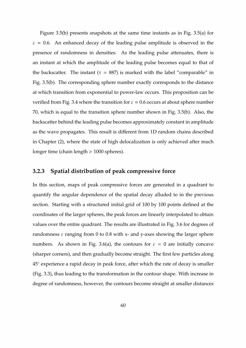
Figure 3.5(b) presents snapshots at the same time instants as in Fig. 3.5(a) for

ε = 0.6. An enhanced decay of the leading pulse amplitude is observed in the

presence of randomness in densities. As the leading pulse attenuates, there is

an instant at which the amplitude of the leading pulse becomes equal to that of

the backscatter. The instant (τ = 887) is marked with the label “comparable” in

Fig. 3.5(b). The corresponding sphere number exactly corresponds to the distance

at which transition from exponential to power-law occurs. This proposition can be

verified from Fig. 3.4 where the transition for ε = 0.6 occurs at about sphere number

70, which is equal to the transition sphere number shown in Fig. 3.5(b). Also, the

backscatter behind the leading pulse becomes approximately constant in amplitude

as the wave propagates. This result is different from 1D random chains described

in Chapter (2), where the state of high delocalization is only achieved after much

longer time (chain length > 1000 spheres).

3.2.3 Spatial distribution of peak compressive force

In this section, maps of peak compressive forces are generated in a quadrant to

quantify the angular dependence of the spatial decay alluded to in the previous

section. Starting with a structured initial grid of 100 by 100 points defined at the

coordinates of the larger spheres, the peak forces are linearly interpolated to obtain

values over the entire quadrant. The results are illustrated in Fig. 3.6 for degrees of

randomness ε ranging from 0 to 0.8 with x- and y-axes showing the larger sphere

numbers. As shown in Fig. 3.6(a), the contours for ε = 0 are initially concave

(sharper corners), and then gradually become straight. The first few particles along

45 experience a rapid decay in peak force, after which the rate of decay is smaller

(Fig. 3.3), thus leading to the transformation in the contour shape. With increase in

degree of randomness, however, the contours become straight at smaller distances

60

from the point of impact because the decay is enhanced in all directions. Also, the

contours transition from straight to approximately circular shape at larger distances,

as visible for ε = 0.4 and ε = 0.8, suggesting an increasingly isotropic nature of the

peak force distribution, as further analyzed in Fig. 3.7.

61

0 20 40 60 80 1000

20

40

60

80

100

= 0

(a)

0 20 40 60 80 1000

20

40

60

80

100

= 0.2

(b)

0 20 40 60 80 1000

20

40

60

80

100

= 0.4

(c)

0 20 40 60 80 1000

20

40

60

80

100

= 0.8

(d)

Figure 3.6: Spatial distribution of total compressive force on larger spheres in thefirst quadrant (x- and y-axis labels are larger sphere numbers) for different degrees ofrandomness, ε, ranging from 0 to 0.8. The results, averaged over sixty realizations,show a transition from concave to straight to convex contour shape as ε and thedistance from the point of impact increase. The white zone depicts forces higherthan 50 N near the initial impact area.

62

0 20 40 60 80 1000

20

40

60

80

100

= 0.2

(a)

0 20 40 60 80 1000

20

40

60

80

100

= 0.4

(b)

0 20 40 60 80 1000

20

40

60

80

100

= 0.6

(c)

0 20 40 60 80 1000

20

40

60

80

100

= 0.8

(d)

Figure 3.7: Spatial distribution (x- and y-axis labels are sphere numbers) of peakcompressive force acting on the larger spheres for different degrees of randomnessnormalized by the force distribution of the nonrandom system.

Focusing on the effect of randomness in densities, Fig. 3.7 shows the spatial dis-

tribution of peak compressive forces for various degrees of randomness normalized

63

by those of the nonrandom system as done previously in Fig. 3.4. As apparent there,

the peak force attenuates more in the 0 and 90 directions, as noted by the steepen-

ing of the contours in these directions. The enhanced attenuation also confirms the

earlier observation in Fig. 3.6 where the contours changed from concave to straight

shape. For smaller distances from the point of impact, as apparent in Fig. 3.7, the

decay is anisotropic while the contours become circular at larger distances for all the

degrees of randomness, indicating the attenuation due to randomness to be isotropic

in this regime.

The anisotropic nature of the decay is further quantified in Fig. 3.8, which shows

the peak force distribution for various angles in the first quadrant for ε = 0.6. As

observed there, the peak forces at smaller distances from the point of impact are

higher for angles close to 0, as was noted in Fig. 3.6. At larger distances, the curves

for all the angles merge, indicating that contours of peak force are approximately

circular leading to the aforementioned isotropic decay.

64

0 20 40 60 80 1000

20

40

60

80

100

120

Distance, x/d

Pea

k fo

rce,

Fm

(N

)

5°

12°

24°

36°

45°

Figure 3.8: Variation of peak force with distance for ε = 0.6 along different directions.The peak forces are essentially the same along all directions at larger distances fromthe point of impact, indicating that the decay becomes increasingly isotropic.

Using the contour maps shown in Figs. 3.6 and 3.7, the decay coefficient αF can

be extracted for different degrees of randomness and various angles θ ranging from

0 to 90 in intervals of 1. For each θ, the peak force values are first interpolated

based on the initially generated peak force values on the 100 by 100 grid. Then

the decay coefficients are extracted by fitting an exponential curve to the peak force

data from a distance from the point of impact equal to about sum of five larger

and smaller bead diameters up to the transition to regime II. Figure 3.9 shows the

dependence of the decay coefficient αF on angle θ for ε = 0.2, 0.4 and 0.6. As

expected, the curves are symmetric about 45, except for small deviations due to

the finite number of realizations. The results demonstrate mainly three different

regions, viz., an initial region of high decay, minimum decay and approximately

65

constant decay. The region of high attenuation for small angles corresponds to

steeper contours at the corners in Fig. 3.7. Then the decay decreases to a minimum

which occurs in the range 15 − 20 for all ε, which can be explained by referring to

the kinks associated with the presence of intersecting wavefronts in the nonrandom

case [51] and denoted by dashed lines in Figs. 3.6(a) and 3.7(c). The decay coefficient

later increases to reach a constant value, as the contours are approximately circular

in this regime where peak force decay of 24, 36 and 45 overlapped (Fig. 3.8). This

decay depends on the underlying granular structure but the anisotropy of decay

will be qualitatively maintained even if the direction of impact is other than 45.

These results identify potential ways to optimize granular systems for objective

functions such as minimizing the rate of decay or inducing an isotropic force decay.

In the absence of intruders, however, the impact event would generate waves that

propagate along 0 and 90 directions [51]. In that case, since wave propagation

is basically 1D, the force decay is expected to be substantially slower than in the

system with intruders.

66

0 10 20 30 40 50 60 70 80 900

0.5

1

1.5

2

2.5

Angle, θ

Dec

ay c

oeffi

cien

t, α F

ε = 0.2ε = 0.4ε = 0.6

Figure 3.9: Decay coefficient αF in the exponential regime as a function of angle θfor different degrees of randomness.

3.2.4 Evolution of ensemble kinetic energy

We now turn our attention to the evolution of ensemble kinetic energy, defined as

the sum of kinetic energies of all the spheres in the system, for various degrees of

randomness. The ensemble kinetic energy gives a measure of the particle vibrations,

while the compressive forces are accounted for by the ensemble potential energy

evaluated by summing the potential energy of each interaction. Since the energy of

the system is conserved, this analysis provides insight on the exchange of energy

between potential and kinetic energies as the wave propagates through the different

regimes discussed earlier. The relevant data is compared with the virial theorem

discussed in Chapter (2), which relates the time-averaged kinetic energy to the time-

averaged potential energy for a system of particles interacting via potentials such

67

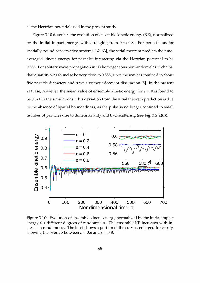
as the Hertzian potential used in the present study.

Figure 3.10 describes the evolution of ensemble kinetic energy (KE), normalized

by the initial impact energy, with ε ranging from 0 to 0.8. For periodic and/or

spatially bound conservative systems [62, 63], the virial theorem predicts the time-

averaged kinetic energy for particles interacting via the Hertzian potential to be

0.555. For solitary wave propagation in 1D homogeneous nonrandom elastic chains,

that quantity was found to be very close to 0.555, since the wave is confined to about

five particle diameters and travels without decay or dissipation [5]. In the present

2D case, however, the mean value of ensemble kinetic energy for ε = 0 is found to

be 0.571 in the simulations. This deviation from the virial theorem prediction is due

to the absence of spatial boundedness, as the pulse is no longer confined to small

number of particles due to dimensionality and backscattering (see Fig. 3.2(a)(i)).

0 100 200 300 400 500 600 700

0.4

0.5

0.6

0.7

0.8

0.9

1

Nondimensional time, τ

Ens

embl

e ki

netic

ene

rgy

ε = 0ε = 0.2ε = 0.4ε = 0.6ε = 0.8

560 580 600

0.56

0.58

0.6

Figure 3.10: Evolution of ensemble kinetic energy normalized by the initial impactenergy for different degrees of randomness. The ensemble KE increases with in-crease in randomness. The inset shows a portion of the curves, enlarged for clarity,showing the overlap between ε = 0.6 and ε = 0.8.

68

With increase in ε, an increase in ensemble KE is observed due to higher

impedance mismatch at contacts. The increase in ensemble KE obtained here is

not as pronounced as in 1D random chains described in Chapter (2) mainly because

of the boundary conditions. In the 1D study, the initial impact sphere was not fixed

and thus the reflected waves caused the first few spheres to freely move away from

the system, leading to enhanced increase in ensemble KE. In the present 2D case,

the impact is provided at the center of the system, and thus the initial spheres are

confined to vibrate with small amplitudes essentially forcing them to stay within the

system. Mean values for different ε are provided in Table 3.1, showing the increase

in ensemble KE with randomness. The role of critical randomness is also apparent

from the table, where we note the values for ε = 0.6 and ε = 0.8 are approximately

the same.

Table 3.1: Computed mean values of ensemble KE normalized by the impact energyfor various degrees of randomness.

Degree of randomness (ε) Mean ensemble KE0 0.571

0.2 0.5780.4 0.5880.6 0.5940.8 0.595

3.3 Conclusions

The effect of randomness in densities on nonlinear wave propagation in 2D granular

systems composed of closely packed spherical particles was investigated numeri-

cally. The two main features of wave propagation in such systems - effect of dimen-

sionality and randomness - were characterized for different levels of randomness.

Force amplitude decay due to dimensionality closely followed a power law, and

a separation of variables was employed to extract the force transmission response

69

due to randomness alone. The resulting variation showed two regimes of decay,

exponential and power law, similar to observations made in 1D random chains.

The transition from exponential to power-law regime occurred when the amplitude

of the leading pulse was equal to that of the backscatter, also consistent with 1D

results. Contours of peak forces on the larger spheres were obtained by linear inter-

polation and contour shapes were characterized for different distances from impact

and degrees of randomness, showing an increasingly isotropic nature of force decay.

Decay in the exponential regime of propagation was quantified by extracting decay

coefficients for various angles, showing regions of minimum or constant decay rate.

Evolution of ensemble kinetic energy was found to be consistent with 1D random

chain, with a progressive increase in kinetic energy.

70

Chapter 4

Plane wave propagation inmonodisperse granular media

In the previous chapters, we studied the effect of randomness on wave propagation

in 1D and 2D granular media. We essentially demonstrated how randomness can

be taken advantage of in applications where energy decay is the key objective.

Randomness was found to enhance the decay due to dimensionality in 2D granular

media. In this chapter, we focus on another practical aspect in applications which

is the loading area. If ordered or disordered granular media were to be deployed in

practical applications, the loading area would likely be spread over a large number

of spheres since the typical diameter of a sphere is of the order of a few millimeters.

The present study complements the work done in previous years on the effect of

point impact on granular layers with spheres arranged in hexagonal packing or

square packing with intruders (see [49, 50, 51, 55]). The focus of our study is on the

other ‘extreme’ loading condition, i.e., uniform planar impact on 2D and 3D periodic

granular media. Qualitatively, randomness is expected to play a similar role as in

the case of point impact and therefore the current study excludes randomness to

specifically address the effect of planar impact.

One of the objectives is to establish an equivalence between a uniformly loaded

2D or 3D granular layer and a 1D chain. Some of the advantages of such a sim-

plification include a drastic reduction in computational cost when simulating large

systems, and a theoretical prediction of the force transmission response of higher-

dimensional structures based on 1D numerical or theoretical results. Another key

objective of the present study is to investigate the mixed compression/shear dynamic

71

response of granular media. In the first part of the study, analytical solutions are

derived for various periodic granular structures such as 2D/3D hexagonal packing

and 3D face-centered cubic packing under uniform perpendicular loading. Owing

to the symmetry and periodic conditions of the domain, the motion of the spheres

is in the direction of impact and the response is thus compared to that of 1D gran-

ular chains. The nonlinear dependence between the wavefront speed and its force

amplitude for 2D and 3D systems are related to that of 1D chains and are found

to be in very good agreement with the simulations. The analytical predictions are

also applicable to dimer systems made up alternating layers of spheres of different

radius or Young’s modulus.

Finally, numerical studies are performed on force transmission response of 2D

hexagonal packing under uniform angular impact. The shearing component in the

impact loading leads to the motion of the spheres in the horizontal direction, but

the shearing effect decays very quickly after just a few layers. The amplitude of

the horizontal component of velocity of the spheres is found to decay exponentially

in the initial layers and further decay in a series of linear regimes with different

decay rates. After the complete decay of shearing effect, the wavefront propagates

in a way similar to that of the perpendicular impact case. A semi-analytical study

based on two layers in contact is adopted to predict the gradual transformation of

direction of propagation of spheres from the impact angle to the perpendicular case.

The present chapter is divided into a number of sections as follows. In Sec. 4.1,

the equations of motion for a granular system and the simulation procedure are

described. Section 4.2 discusses the normal impact case for 2D and 3D granular

media and provides analytical derivation and verification (Secs. 4.2.1 and 4.2.2)

for the equivalent 1D chains. Section 4.3 describes the angular impact case. The

numerical observations are discussed in Sec. 4.3.1, while Sec. 4.3.2 reports analytical

predictions for some of the key phenomena observed in the angular impact case

72

and a comparison with numerical results. The results of the above study has been

published in Granular Matter (”Plane wave propagation in 2D and 3D monodisperse

periodic granular media.” Granular Matter 16.1 (2014): 141-150) and the remainder

of this chapter follows in most part that publication.

4.1 Numerical setup

In this study, various 2D and 3D ordered granular packings made up of elastic

monodisperse spherical particles are considered. Initial conditions in the form of

velocity impulses transmit compressive pulse(s) in the domain. The equations of

motion for sphere i and definitions for the relevant parameters are given in Sec. 3.1.

Figure 4.1 shows the four packings investigated in the present study: 2D hexag-

onal (Fig. 4.1(a)), 3D face-centered cubic (Fig. 4.1(b)), 3D hexagonal close packing

(Fig. 4.1(c)) and 3D body-centered cubic packing (Fig. 4.1(d)). The spheres in the

topmost layer are given an initial impact velocity of magnitude vp0 along direction

θ as shown. In the following sections, the analysis is divided into two cases, viz.,

planar perpendicular (or normal) impact (θ = 90) and angular impact (arbitrary

θ). We model the systems using periodic boundary conditions in the direction(s)

‘x’ for 2D and ‘x’ and ‘y’ for 3D packings. The prominent direction of propagation

of compressive pulses (‘y’ in 2D and ‘z’ in 3D) is modeled as a semi-infinite system,

i.e., the transmission response is free from the influence of the boundary.

73

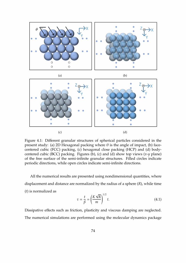
(a) (b)

(c) (d)

Figure 4.1: Different granular structures of spherical particles considered in thepresent study: (a) 2D Hexagonal packing where θ is the angle of impact, (b) face-centered cubic (FCC) packing, (c) hexagonal close packing (HCP) and (d) body-centered cubic (BCC) packing. Figures (b), (c) and (d) show top views (x-y plane)of the free surface of the semi-infinite granular structures. Filled circles indicateperiodic directions, while open circles indicate semi-infinite directions.

All the numerical results are presented using nondimensional quantities, where

displacement and distance are normalized by the radius of a sphere (R), while time

(t) is normalized as

τ =t

β=

(K√

R

m

)1/2

t. (4.1)

Dissipative effects such as friction, plasticity and viscous damping are neglected.

The numerical simulations are performed using the molecular dynamics package

74

LAMMPS [61] by considering spheres as point masses connected by nonlinear

springs. Time step is chosen as τ ≈ 3.55 × 10−3. The total energy and linear

momentum are conserved with a relative error less than 10−7 and 10−12, respectively.

4.2 Normal impact

Consider different granular packings under uniform planar impact as shown in

Fig. 4.1, whereθ is the angle of impact. In this section, normal impact (θ = 90) is con-

sidered, and the periodic conditions imply that y-displacements (z-displacements)

are the only nonzero components in 2D (3D) packings since all the spheres in each

layer have equal displacements. The foregoing discussion applies to 2D hexagonal

packing but can be generalized to 3D.

4.2.1 Analytical study

In order to predict analytically the force propagation response due to normal impact,

one needs to first derive the equations of motion of a sphere for any packing. The

forces acting on a sphere are obtained using the Hertzian contact law, with the

deformation at a contact defined as follows: Let δi−1,i be the relative displacement

between two neighboring spheres (in layers i − 1, i) located at (x1, y0i−1) and (x2,

y0i), respectively. If the corresponding y-displacements for these two spheres are

denoted by vi−1 and vi, then

δi−1,i =

√(x2 − x1)2 + (y0i − y0i−1)2

−√

(x2 − x1)2 + (y0i − y0i−1 + vi − vi−1)2

= 2R −√

4R2 + 2(y0i − y0i−1)(vi − vi−1) + (vi − vi−1)2.

(4.2)

75

By assuming that the displacements are much smaller than the radius (R), one gets

δi−1,i ≈ 2R

1 −

√1 − (y0i − y0i−1)

2R2(vi−1 − vi)

≈ (y0i − y0i−1)

2R(vi−1 − vi).

(4.3)

In Eq. (4.3), (y0i − y0i−1) corresponds to the distance between adjacent layers, and

thus its value depends on the packing under consideration. For example, for 2D

hexagonal packing, the value is√

3R, and similar values can be found for other

packings. The contact force magnitude F (valid for spheres under compression) is

given by

Fi−1,i = Kδ3/2i−1,i= (4/3)E∗

√R∗δ3/2

i−1,i, (4.4)

where E∗ and R∗ were defined in Sec. 4.1. The equation of motion for a sphere of

mass m can then be written by considering all the contact forces. For 2D hexagonal

packing, Eq. (4.3) yields

vi =√

3K

m(δ3/2

i−1,i− δ3/2

i,i+1) (4.5)

=√

3

( √3

2

)3/2

A[(vi−1 − vi)3/2 − (vi − vi+1)3/2], (4.6)

with A = 2E/(πρ(1−ν2)(2R)5/2), where ρ is the density of the particles. Equation (4.6)

is indeed very similar to the equation of motion for a sphere in a 1D homogeneous

chain with the factor f =√

3(√

3/2)3/2 in Eq. (4.6) replaced by unity [5]. The above

1D equivalence also holds if the adjacent layers have different Young’s moduli or

radii (assuming packing remains the same), in which case an appropriate value of

E∗ or R∗ should be used in K.

To derive the constant factor in the nonlinear dependence between the wavefront

speed and the force amplitude in the 2D hexagonal system, a scaling analysis is

76

employed. Nesterenko’s continuum approximation to the 1D chain of spheres

[5] provides the scaling relation between the strain (ξ), the wave speed (V) and

the factor f . This continuum definition of wave speed, which arises from traveling

wave assumption, is calculated in the discrete case by monitoring the time difference

between peak forces or velocities at adjacent contacts. Since the strain in the system

is equal to the particle velocity (vp) divided by the wave speed, one gets the relations

ξ2D =1

f 2

V42D

V41D

ξ1D ⇒ vp2D =1

f 2

V52D

V51D

vp1D. (4.7)

Finally, the force amplitude (Fm) and the strain amplitude (ξm) are related by

Fm = Kδ3/2 ≈ K(2R)3/2ξ3/2m , (4.8)

where the deformed length is assumed to be approximately the strain times the

diameter of a sphere. Using Eqs. (4.3), (4.7) and (4.8), one obtains

Fm2D

Fm1D=

( √3

2

)3/2ξ3/2

m2D

ξ3/2m1D

=

( √3

2

)3/21

f 3

V62D

V61D

. (4.9)

We now define the wavefront speed (V) as the component of the wave speed (V)

along the direction of propagation. For example, for the 2D hexagonal packing,

V = Vsin(60) = (√

3/2)V. Employing the nonlinear dependence between the wave

speed and the force amplitude for 1D chains, V = BF1/6m [22], where

B ≈(

384

125π3

)1/6(

E

Rρ3/2(1 − ν2)

)1/3

, (4.10)

we get

V2D =3

2√

2BF1/6

m2D. (4.11)

77

Similarly, force-wavefront speed relations for the 3D systems of the present study

are

VFCC =2√3

BF1/6mFCC

and VBCC = BF1/6mBCC. (4.12)

We note that the response of the HCP system will be equal to that of the FCC packing

due to periodic boundary conditions in the in-plane directions.

4.2.2 Verification

Figure 4.2 shows the dependence of the wavefront speed and the force amplitude

for various granular configurations. Numerical results are compared with the ana-

lytical predictions from the previous section along with results for a 1D chain. The

wavefront speed and force amplitude are normalized as

V =β

RV =

(m

KR5/2

)1/2

V and Fm =Fm

KR3/2, (4.13)

respectively. As apparent there, the analytical predictions are in very good agree-

ment with the simulations. As alluded to in Eq. (4.12), the wavefront speed for the

3D BCC packing is exactly equal to the corresponding 1D chain, thus is represented

by the same analytical curve in Fig. 4.2.

78

0 2 4 6 8

x 10−4

0.25

0.3

0.35

0.4

0.45

0.5

0.55

0.6

Force amplitude (Fm)

Wav

efro

nt

spee

d(V

)

1D Simulations2D Hexagonal − Analytical2D Hexagonal − Simulations3D FCC − Analytical3D FCC − Simulations3D BCC − Simulations1D, 3D BCC − Analytical

Figure 4.2: Normalized wavefront speed (V) versus force amplitude (Fm) for differentgranular systems. Solid curves correspond to the analytical relations Eq. (4.11) and(4.12) and symbols to numerical results. Note that a 3D BCC system and the 1D

homogeneous chain show equivalent responses. V and Fm are defined in Eq. (4.13).

4.2.3 Normalization

The aforementioned equations of motion and scaling relations point to two parame-

ters governing the constant factor entering the wave speed-force amplitude relations

(Eqs. (4.11)-(4.12)). One is given by the number of contacts nc between a sphere and

an adjacent layer, and the other is the height h equal to the distance between adjacent

layers. The scaling relations discussed in the previous section yield

V

n1/2c h2

=βK1/6

R3/4BF1/6

m , (4.14)

79

where B is given by Eq. (4.10) and h = h/(2R). For 2D hexagonal packing, nc = 2 and

h =√

3/2, and thus one recovers the wavefront speed relation in Eq. (4.11). Figure

4.3 demonstrates the normalized wavefront speed (V/(n1/2c h2)) as a function of its

force amplitude (Fm) where all the curves previously separated in Fig. 4.2 collapse

onto one curve, verifying the normalization described by Eq. (4.14).

0 2 4 6 8

x 10−4

0.25

0.3

0.35

0.4

0.45

0.5

0.55

0.6

Force amplitude (Fm)

Wav

efro

nt

spee

d(V

/(n

1/2

ch

2))

1D Simulations2D Hexagonal − Simulations3D FCC − Simulations3D BCC − Simulations1D, 2D, 3D − Analytical

Figure 4.3: Normalized wavefront speed (V/(n1/2c h2)) as a function of force amplitude

(Fm) given by the scaling relation in Eq. (4.14). All the curves in Fig. 4.2 collapse tothe normalized curve.

4.3 Angular impact: 2D hexagonal packing

In this section, we discuss the force transmission response of a 2D hexagonal packing

under angular impact, i.e., 0 ≤ θ < 90 (Fig. 4.1(a)). The key difference between the

80

angular impact and the normal impact is the presence of the shearing component in

the former, with θ = 0 corresponding to pure shear. Consequently, the spheres are

expected to have also a motion in the horizontal (‘x’) direction.

4.3.1 Numerical observations

Consider a 2D hexagonal packing with impact angle θ = 60. Figure 4.4 illustrates

the history of the contact forces between neighboring layers as the disturbance

propagates in the system. The contact forces labeled I and II correspond to the

two distinct contacts taking place between any two layers as shown in the inset of

Fig. 4.4. As expected, the force of contact I is initially lower than that of contact II as

illustrated by the curves labeled ‘layers 1-2’. However, the contact I force increases

with depth while the contact II force decreases. As apparent in Fig. 4.4, the forces

at contacts I and II become identical after a certain depth. The mechanism for the

transformation of contact forces is explained as follows. For any θ, the presence of

the contact forces between layers ‘1’ and ‘2’ induce layer ‘2’ to start its motion along

some θ ≥ 60 since the line joining the centers is along θ = 60. Consequently, each

successive layer starts its motion along an angle greater than the previous layer,

gradually changing the direction of motion from the impact angle θ to 90 after a

certain depth, where the forces at the two contacts become equal. The scenario is

then similar to that of the normal impact case.

81

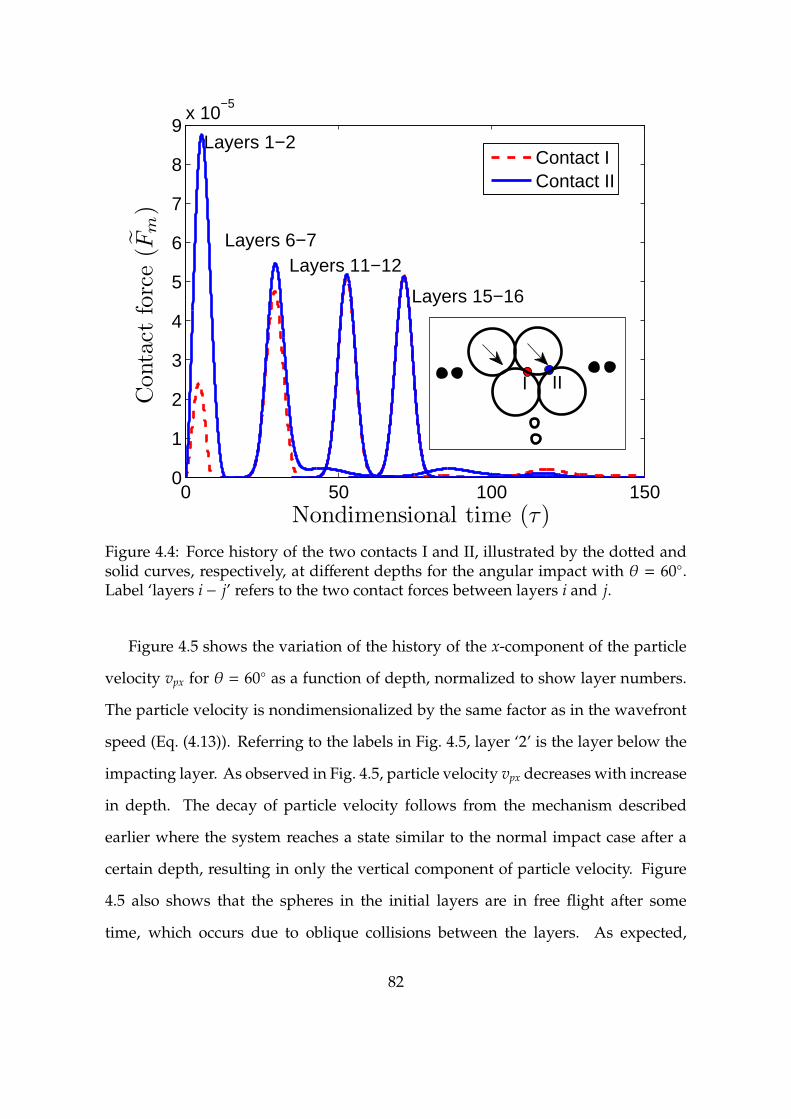
0 50 100 1500

1

2

3

4

5

6

7

8

9x 10

−5

Nondimensional time (τ)

Con

tact

forc

e(F

m)

Contact IContact II

Layers 1−2

Layers 6−7Layers 11−12

III

Layers 15−16

Figure 4.4: Force history of the two contacts I and II, illustrated by the dotted andsolid curves, respectively, at different depths for the angular impact with θ = 60.Label ‘layers i − j’ refers to the two contact forces between layers i and j.

Figure 4.5 shows the variation of the history of the x-component of the particle

velocity vpx for θ = 60 as a function of depth, normalized to show layer numbers.

The particle velocity is nondimensionalized by the same factor as in the wavefront

speed (Eq. (4.13)). Referring to the labels in Fig. 4.5, layer ‘2’ is the layer below the

impacting layer. As observed in Fig. 4.5, particle velocity vpx decreases with increase

in depth. The decay of particle velocity follows from the mechanism described

earlier where the system reaches a state similar to the normal impact case after a

certain depth, resulting in only the vertical component of particle velocity. Figure

4.5 also shows that the spheres in the initial layers are in free flight after some

time, which occurs due to oblique collisions between the layers. As expected,

82

0 50 100 150 200 250 300 3500

0.2

0.4

0.6

0.8

1

1.2

1.4

1.6

1.8x 10

−4

Nondimensional time (τ)

Par

ticl

ehor

izon

talvel

oci

ty

40 60 80 1000

1

2

3

x 10−5

Layer 4

Layer 3

Layer 2

Figure 4.5: History of the x-component of particle velocity as a function of depth(layers) for θ = 60 showing a rapid decay in amplitude and the appearance ofsecondary peaks.

the horizontal component of the free-flight velocity ceases to exist after a certain

depth. Furthermore, there is formation of secondary waves after few layers, the

consequence of which will be discussed shortly.

Figure 4.6 shows the variation of the peak amplitude of vpx as a function of depth,

extracted from Fig. 4.5. As apparent in Fig. 4.6, there are several regimes of decay

in peak amplitude, as indicated by the labels ‘R1’ to ‘R4’. The solid vertical lines

mark the transition between different regimes. A simple curve fit demonstrates that

the regime ‘R1’ is very well described by an exponential decay while the regimes

‘R2’ to ‘R4’ are described by a linear decay. As seen in Fig. 4.5, secondary waves

decay slower than the primary waves leading to higher amplitude of the former

83

after a certain depth. Similar secondary waves lead to the formation of other linear

regimes. Although it appears that the transition has to be function of the primary

wave’s spatial width, the exact source is yet to be ascertained. As observed in the

inset of Fig. 4.5, secondary waves begin to form at a certain depth. As the primary

wave regime ‘R1’ decays exponentially, there is a layer at which the secondary

wave’s amplitude becomes higher than that of the primary wave. However, the

primary wave’s amplitude continues to decay exponentially, as indicated by the

square markers in Fig. 6, while the peak is dictated by the secondary regime

(circular markers). The above explanation holds for the transition between ‘R2’ and

‘R3’ regimes as well, as indicated by the triangular markers in Fig. 4.6.

84

0 5 10 15 20 25 30

10−6

10−5

10−4

Layer number

Part

icle

vel

oci

tyam

plitu

de

Peak amplitudeR

1 amplitude

R2 amplitude

R1

R2

R3

R4

θ = 60o

Figure 4.6: Variation of peak amplitudes of particle velocity vpx with depth demon-strating various regimes of decay R1 to R4. Regimes with square and triangularmarkers show amplitudes of R1 and R2, respectively, after the secondary wavesgovern the peak amplitude (Fig. 4.5).

Figure 4.7 illustrates the dependence of the wavefront speed on the contact force

amplitude for various impact angles. We note that the wavefront refers to the lead-

ing pulse that propagates after the shearing component decays completely. Thus,

the relations derived earlier for the normal impact case can be employed for wave-

front speed prediction. The solid curve in Fig. 4.7 corresponds to the approximate

analytical dependence given by Eq. (4.11), or equivalently the normalized curve in

Fig. 4.3. As expected, there is a good agreement between the simulations and the

analytical prediction. As the impact angle θ decreases, the force amplitude and the

wavefront speed decrease since more energy is contributed to the horizontal motion

85

of the spheres in the initial few layers, as discussed earlier.

0 0.2 0.4 0.6 0.8 1

x 10−4

0.24

0.26

0.28

0.3

0.32

0.34

0.36

Force amplitude (Fm)

Wav

efro

nt

spee

d(V

/(n

1/2

ch

2))

SimulationsAnalytical

θ

θ = 0o

θ = 90o

Figure 4.7: Wavefront speed as a function of its force amplitude for the 2D hexagonalpacking for various impact angles θ ranging from 0 to 90, comparing with theanalytical (solid) normalized curve of Fig. 4.3.

4.3.2 Analytical predictions

Amplitude of leading pulse

The force amplitude of the leading pulse can be predicted by estimating the energy

carried by the leading pulse after the impact of the topmost layer. To this end,

consider a two-layered periodic system of hexagonal packing as shown in Fig. 4.8.

The layer marked ‘1’ impacts layer ‘2’ at an angle θ to the horizontal, while layer

‘2’ is free to move. The velocity of the second layer after impact can be obtained

86

for angles 0 ≤ θ ≤ 30, where the problem is equivalent to an oblique impact of

two spheres. The free-flight velocity of the second layer after impact can then be

obtained by the conservation of linear momentum and energy as

vp2 = vp0 cos(60 − θ) =vp0

2

(cosθ +

√3 sinθ

), (4.15)

where vp0 is the initial velocity magnitude of the topmost layer and θ is as defined

in Fig. 4.1(a). Let us assume that the kinetic energy carried by the second layer in

the above analysis is approximately equal to the energy carried by the leading pulse

(denoted by Eθ) in the infinite-layer system. We then obtain

Eθ ∝ v2p2 =

v2p0

4

(3 − 2cos2θ +

√3 sin 2θ

). (4.16)

Figure 4.8: Two-layered hexagonal packing periodic in x-direction used in theoreticalprediction of shear decay, and the resulting contact forces (marked F1 and F2) on thespheres in layers ‘1’ and ‘2’. Layer ‘1’ impacts at an angle θ to the horizontal andlayer ‘2’ is free to move.

87

The energy Eθ in Eq. (4.16) can be normalized with that of the normal impact

case (E0), for which the entire impact energy is transmitted (neglecting the small

initial reflection), i.e., E0 ∝ v2p0. Finally, we introduce the scaling relation between

the energy and the force amplitude of a solitary wave, E ∝ F5/3m . The force amplitude

of the leading pulse when 0 ≤ θ ≤ 30 (Fmθ) normalized by that of the normal

impact (Fm0) is then given by

Fmθ

Fm0≈

[1

4

(3 − 2cos2θ +

√3 sin 2θ

)]3/5

. (4.17)

Figure 4.9 shows a comparison between the force amplitude-impact angle depen-

dence of the leading pulse obtained numerically and that described by Eq. (4.17). We

find a good agreement between the simulations and the analytical result for angles

θ ≤ 30 (left of dashed line), as expected. For θ > 30, the spheres in the topmost

layer will form two contacts with the corresponding spheres in the second layer,

rendering the approximation (4.17) inapplicable. The analytical prediction gives an

upper bound because the infinite-layer system “loses” energy at every interface of

initial few layers due to oblique impact, whereas the analytical prediction accounts

for only two layers. Nevertheless, the bulk of the rebound energy is carried by the

topmost layer, as also confirmed by Fig. 4.9.

88

0 20 40 60 80 1000.4

0.5

0.6

0.7

0.8

0.9

1

1.1

Impact angle (θ)

For

ceam

plitu

de

(Fm

θ/F

m0)

PredictionSimulations

Figure 4.9: Force amplitude of the leading pulse for various impact angles θ (Fmθ)normalized by that of normal impact case (Fm0). The dashed line denotes the maxi-mum value of θ (= 30) for which the theoretical prediction (4.17) is expected to bevalid.

Shear component decay

In Sec. 4.3.1, we discussed the rapid attenuation of the shearing effect and Fig. 4.6

showed the rate of decay of the x-component of the particle velocity with depth.

In this section, an iterative procedure based on the two-layered model (Fig. 4.8) is

employed to predict the decay of the shearing effect. The idea is to find the direction

of travel (based on acceleration vector) of layer ‘2’, which would then be considered

as layer ‘1’ (coming at the new θ) in the second iteration. The above steps are

repeated until the shearing component has decayed, i.e., until the impacted layer

89

‘2’ travels at an angle within a specified tolerance of 90, which corresponds to the

normal impact case.

Let us define α as the angle the force (or acceleration) vector of layer ‘2’ in Fig. 4.8

makes with the horizontal. Writing the force vector with components Fx and Fy as a

function of the contact forces F1 and F2, one gets

tanα =Fy

Fx=√

3(F1 + F2

F2 − F1

). (4.18)

Then consider the force-particle velocity scaling relation given by F ∝ v6/5p , where

F is the contact force between any two spheres and vp is the velocity of approach

(defined as the difference between the two velocities). In Fig. 4.8, let the initial

velocity magnitude of layer ‘1’ be vp0. As a first approximation, let us neglect the

coupling effect of the two contact forces F1 and F2 and write the scaling relations

independently. Thus, the velocities of approach for the two contact forces F1 and F2

are vp0cos(120 − θ) and vp0cos(60 − θ), respectively, leading to

F1 ∝ [vp0 cos(120 − θ)]6/5

F2 ∝ [vp0 cos(60 − θ)]6/5.(4.19)

Equation (4.18) becomes

tanα ≈√

3

([cos(60 − θ)]6/5

+ [cos(120 − θ)]6/5

[cos(60 − θ)]6/5 − [cos(120 − θ)]6/5

). (4.20)

In the second iteration, the α from Eq. (4.20) is taken as the new θ, where

layer ‘2’ impacts layer ‘3’ and so on. Figure 4.10 illustrates the variation of angle

α with depth (or layer number) comparing the results from the above iterative

procedure (labeled ‘prediction’) with those of the simulations for two initial angles

of impact θ = 60 and θ = 80. Simulations correspond to the full system in

90

Fig. 4.1(a), and α is calculated at the time step when the particles start moving in

each layer. Overall, the analytical predictions and simulations agree reasonably well,

particularly the analytical predictions for the distance to approach 90 correspond

very well with the simulations. Small differences observed arise from the fact that

there is coupling effect between the two contact forces (F1 and F2) and the analytical

procedure considers only two layers at a time.

2 4 6 8 10 1260

65

70

75

80

85

90

Layer number

Angl

e(α

)

Semi−analyticalSimulations

θ = 60

θ = 80

Figure 4.10: Semi-analytical predictions for the two-layered system of Fig. 4.8, show-ing the angle α as a function of depth for two different impact angles: θ = 60 andθ = 80. Simulations consider the full domain of Fig. 4.1(a).

91

Exponential regime decay rate

In this section, another iterative procedure is developed to predict the decay rate

of the exponential regime, as observed in Fig. 4.6. As before, we consider the two-

layered periodic system of hexagonal packing as shown in Fig. 4.8. Here, a set

of ordinary differential equations are obtained to predict the free-flight velocity of

layer ‘2’, and the procedure is repeated iteratively. The exponential decay rate is

then determined based on the ratio of final x-velocity of layer ‘2’ to initial x-velocity

of layer ‘1’ at each iteration.

Let ui and vi be the x- and y-displacements of ith layer (i = 1, 2). The equations of

motion are therefore given by

mu1 =1

2(F1 − F2), mu2 =

1

2(F2 − F1),

mv1 = −√

3

2(F1 + F2), mv2 =

√3

2(F1 + F2).

(4.21)

For convenience, let us define new variables u = u1 − u2 and v = v1 − v2. The

Eqs. (4.21) reduce to

mu = F1 − F2,

mv = −√

3(F1 + F2).(4.22)

The contact forces F1 and F2 can be written in terms of the displacements by using

Eq. (4.4), where the relative displacement δ is derived similar to Eq. (4.3) by including

92

x-displacements as well. Finally, one gets

F1 = K[1

2

(u2 − u1 +

√3v1 −

√3v2

)]3/2

=K

23/2

(−u +

√3v

)3/2,

F2 = K[1

2

(u1 − u2 +

√3v1 −

√3v2

)]3/2

=K

23/2

(u +√

3v)3/2.

(4.23)

Substituting Eqs. (4.23) in the reduced equations of motion (Eq. (4.22)) leads to

mu =K

23/2

[(−u +

√3v

)3/2−

(u +√

3v)3/2

],

mv = −√

3K

23/2

[(−u +

√3v

)3/2+

(u +√

3v)3/2

].

(4.24)

We can now consider the Taylor series expansion of the right hand side of Eqs. (4.24)

with the assumption that√

3v ≫ u, later shown to be a good assumption. The first

Eq. (4.24) yields

u =K

m

(√

3v)3/2

23/2

(1 − u√

3v

)3/2

−(1 +

u√3v

)3/2

=K

m

(√

3v)3/2

23/2

[−3

u√3v+ O

(u3

v3

)]. (4.25)

Similarly, the second Eq. (4.24) can be rewritten as

v = −K

m

√3(√

3v)3/2

23/2

(1 − u√

3v

)3/2

+

(1 +

u√3v

)3/2

= −K

m

√3(√

3v)3/2

23/2

[2 +

1

4

u2

v2+ O

(u4

v4

)]. (4.26)

Retaining terms up to second order in u/v, the final form of the system of ordinary

93

differential equations (ODEs) is

u ≈ −35/4

23/2

K

m

(u√

v),

v ≈ −35/4

23/2

K

m

(2v3/2 +

1

4u2v−1/2

).

(4.27)

This system of coupled ODEs is then numerically integrated to obtain the evo-

lution of the displacement variables (u and v) and the velocity variables (u and v).

The initial conditions are chosen corresponding to vp0 = 1 m/s (vp0 = 5.6336 × 10−4

in nondimensional units) and θ = 60, leading to

u(0) = 0, u(0) = vp0cos(θ),

v(0) = 0, v(0) = vp0sin(θ).(4.28)

Figures 4.11 and 4.12 show the evolution of displacement and velocity variables,

respectively, and compare the solution of the ODEs (Eq. (4.27)) to those of the discrete

simulations, showing a very good agreement. We are particularly interested in the

velocity variable u to predict the decay rate of x-velocity, and thus we can proceed

with the iterative procedure described earlier to obtain the exponential decay rate.

We also note that, in Fig. 4.12, the final value of the velocity variable v from the ODEs

is slightly different from that of the simulations. There are mainly two sources of this

deviation. Firstly, the initial assumption that√

3v ≫ u breaks down after a certain

time in the displacement variable v (Fig. 4.11). And secondly, one of the contacts in

Fig. 4.8 will separate before the other, and hence the system of equations (4.21) may

not fully capture this effect.

94

0 2 4 6 8 10 12−1

−0.5

0

0.5

1

1.5

2x 10

−3

Time (τ)

Dis

pla

cem

ent

vari

able

s

u (simulations)

v (simulations)

u (ODEs)

v (ODEs)

Figure 4.11: History of displacement variables u and v showing a comparison be-tween the solution of the ODEs in Eq. (4.27) and that of the simulations for the sametwo-layered structure (Fig. 4.8).

95

0 2 4 6 8 10 12−6

−4

−2

0

2

4

6x 10

−4

Time (τ)

Vel

oci

tyva

riable

s

u (simulations)

v (simulations)

u (ODEs)

v (ODEs)

Figure 4.12: History of velocity variables u and v from the simulation of Fig. 4.8 andnumerical solution of the ODEs (4.27).

Let us extract the free flight x-velocity of layer ‘1’ and ‘2’ (u1 and u2) by employing

the conservation of linear momentum and the final asymptote value for u in Fig. 4.12.

The relevant equations for iteration i are

u1i+ u2i

= u2i−1,

u1i− u2i

= ui,(4.29)

where u20= 2.8168 × 10−4. Then the ratio q = u2i

/u2i−1gives a measure of the

96

exponential decay rate (r, defined as u2(y) ∝ exp[−ry]) as given by

q =u2i

u2i−1

≈ e−r√

3Ri

e−r√

3R(i−1)= e−r

√3R. (4.30)

The results for the first three iterations are tabulated in Table 4.1. For the nu-

Table 4.1: Decay rate at each iteration from the solution of the ODEs (4.27).

Iteration u2i−1(×10−4) u2i

(×10−4) q = u2i/u2i−1

r1 2.8168 1.8889 0.6706 46.142 1.8889 1.2664 0.6704 46.173 1.2664 0.8490 0.6704 46.17

merical results, an exponential curve fit to the regime R1 in Fig. 4.6 gives a decay

rate r = 42.61 m−1. Thus the analytical predictions in Table 4.1 approximately differ

by 8% from the numerical results. One can possibly reduce the error by taking

higher-order terms in the ODEs (4.27).

4.4 Conclusions

Numerical and theoretical studies were performed on the effect of uniform impact

on wave propagation in 2D and 3D periodic monodisperse elastic granular media

such as hexagonal, FCC and BCC structures. For the normal impact case, equivalent

1D chains based on theoretical considerations were obtained for the 2D and 3D

granular structures. In particular, relations between the wavefront speed and its

force amplitude for the 2D and 3D structures were found to be similar to that of a

homogeneous chain. Furthermore, the analytical solutions were found to be in very

good agreement with the numerical results, and an universal normalized relation

between the wavefront speed and its force amplitude was found to be valid for all

the granular structures considered in the present study.

Studies on angular impact of 2D hexagonal packing were also investigated to

97

understand the effect of shear loading. Numerical study revealed that the shearing

effect attenuates quickly to a state similar to that of the normal impact case. Further,

the amplitude of the horizontal (shear) component of particle velocity was found to

decay in several regimes such as an initial exponential regime and later a series of

linear regimes. By employing a simplified two-layered model, several theoretical

considerations showed good comparison with the simulations. The force amplitude

of the leading pulse (for a limited range of impact angle) was predicted by determin-

ing energy of the leading pulse and then using the energy-force scaling relation. The

direction of propagation of each layer was predicted by applying the force-particle

velocity scaling relation, demonstrating rapid shift to the normal impact state. Fi-

nally, the exponential regime decay rate was determined based on an approximate

system of ODEs for the two-layered system.

In closing, it should be mentioned that the energy dissipation associated with

friction would lead to a higher decay rate of the shear component of the force

and velocity. The value of the decay rate obtained in the present study therefore

corresponds to a lower bound.

98

Chapter 5

Plane wave propagation in dimergranular media

One of the limitations of the monodisperse granular media is that the system always

gives rise to energy-preserving solitary waves. We can only have the capability

of changing the magnitude of the response based on the geometric and material

properties. In order to obtain a different response, i.e., an energy-decaying response,

we need to introduce a second set of spheres with different geometric and material

properties. Few studies on dimer granular chains have successfully shown the

capability to change the response from a solitary wave to energy-decaying wave

[39]. The following work elicits motivation from dimer chains and extends the

study on plane wave propagation in monodisperse granular media (Chapter 4) to

bidisperse granular media to derive more flexibility in altering the response of the

system. In the present study, we perform a numerical and theoretical investigation

of plane wave propagation in square packing granular media with intruders at

interstitial locations. We explore the existence of an equivalent 1D ’nonlocal chain’

for the bidisperse system and carry out numerous simulations to systematically

investigate plane wave propagation behavior. We demonstrate the existence of a

new set of solitary waves in periodic dimer granular crystals. The current study

also demonstrates different ways in which the bidisperse system can help mitigate

or preserve the force amplitude of the wave.

For the square packing system with intruders at interstitial positions, an equiv-

alent 1D chain has been identified analytically and verified with numerical simula-

tions. The system is normalized to obtain two nondimensional parameters which

99

are functions of mass ratio between the larger and smaller spheres and stiffness

ratio between the two types of contacts, respectively. We find that there is one set

of discrete combinations of the nondimensional parameters for which there is max-

imum decay of force amplitude while there is another set of values that preserve

the original impulse. The latter case is particularly interesting where the square

packing system allows solitary waves for certain discrete combinations although

the system is inhomogeneous. Out of several solitary waves possible, there is one

case where the velocity profiles of both larger and smaller spheres are similar to that

of a homogenous chain. Some analytical procedures similar to that of homogeneous

chains such as quasi-continuum approach and asymptotic analysis are considered to

predict the wavefront speed and wave width, and the theoretical results show good

agreement with the numerical simulations. Eight distinct solitary waves have been

systematically extracted from the simulations to construct a ‘solitary wave map’

illustrating the nondimensional parameters that give rise to each of these waves.

The following sections form the remainder of the chapter: Section 5.1 provides

the problem statement and its numerical implementation. In Sec. 5.2.1, we determine

an equivalent 1D chain for the bidisperse system and verify its formulation. Sections

5.2.2 and 5.2.3 summarize some of the key numerical observations. In Sec. 5.3,

analytical techniques such as the quasi-continuum approximation and an asymptotic

analysis are used to predict some of the key phenomena observed numerically. The

results of the above study has been published in the journal Physical Review E

(”Family of plane solitary waves in periodic dimer crystals.” Physical Review E 90.3

(2014): 032209) and the remainder of this chapter follows in most part that reference.

100

5.1 Problem statement

Consider a square packing system of spherical particles with spherical intruders

placed at interstitial locations as shown in Fig. 5.1(a). The granular system is periodic

in the lateral direction (‘x’) and ‘semi-infinite’ in the longitudinal direction (‘y’) so

that the system is free from boundary effects. The equations of motion for sphere

i and the definitions of the involved variables are given in Sec. 3.1. Because of

the closed-packed nature of the system, the intruder spheres can have a maximum

of four neighboring contacts while the main (larger) spheres can have upto eight

contacts.

For the square packing system, the ratio of the radius of a smaller sphere (R2) to

a larger sphere (R1) is√

2− 1. The material properties of the spheres such as density

(ρ1, ρ2), Young’s modulus (E1, E2) and Poisson’s ratio (ν1, ν2) and the geometrical

properties may vary based on the nondimensional parameters that will be discussed

in the next section. All the spheres are assumed to be elastic and dissipative effects

such as friction and damping are neglected. The simulations are performed using

the molecular dynamics code LAMMPS (Large-scale Atomic/Molecular Massively

Parallel Simulator) [61], where the spheres are interpreted as point masses while the

contacts are simulated using nonlinear springs. An in-house code is also developed

to simulate the dynamics in 1D granular chains, where the time integration is per-

formed using the fourth-order Runge-Kutta method. The square packing system is

then given a uniform perpendicular impact of velocity magnitude vp0 as shown in

Fig. 5.1(a). Quantities such as the velocity of the particles and the force amplitude

at various contacts are monitored during the simulations.

101

(a) (b)

Figure 5.1: (a) 2D square packing system of spheres with spherical intruders atinterstitials. Arrows on the topmost layer indicate the planar initial velocity impulse.Periodicity is enforced in the x-direction while y-direction is semi-infinite. (b) The1D chain with nonlocal interactions proposed as equivalent to the 2D system.

5.2 Numerical Results

5.2.1 Equivalent 1D system

Due to the periodicity enforced in the x-direction and the impact being planar per-

pendicular, the forces on the particles are symmetric with respect to the y-axis and

thus the particles have displacements in the y-direction alone. Thus the govern-

ing equations of motion in the y-direction for the 2D square packing system with

102

intruders (Fig. 5.1(a)) are given by

m1 ¨ui =√

2K2

(R1

R1 + R2

)3/2 [(ui−1 − ui)

3/2 − (ui − ui+1)3/2]

+ K1

[(ui−2 − ui)

3/2 − (ui − ui+2)3/2],

m2 ¨ui+1 =√

2K2

(R1

R1 + R2

)3/2 [(ui − ui+1)3/2 − (ui+1 − ui+2)3/2

],

(5.1)

where K1 and K2 are the contact stiffnesses for main-main and main-intruder spheres

interactions, respectively, while m1 and m2 are the masses of the larger beads with

displacements ui and ui±2 and intruder beads with displacements ui±1, respectively.

The vertical displacement (u) and time (t) variables are nondimensionalized as

u =u

R1

and τ =t

(m1

K1

√R1

)1/2, (5.2)

respectively, where u and τ are corresponding nondimensional variables. The equa-

tions of motion (5.1) can now be written in a nondimensional form, with the two

parameters governing the dynamics of the system defined by

ε =m2

m1and α =

2−1/4K2

K1. (5.3)

All the results reported herein are valid for a wide range of material properties

depending on the nondimensional parameters in Eq. (5.3). One can now write the

equations of motion in nondimensional form as

ui =α[(ui−1 − ui)

3/2 − (ui − ui+1)3/2]+

+[(ui−2 − ui)

3/2 − (ui − ui+2)3/2],

εui+1 =α[(ui − ui+1)3/2 − (ui+1 − ui+2)3/2

].

(5.4)

Since the system is periodic, the dynamics is essentially one-dimensional and

103

therefore one can think of an equivalent 1D chain that would give the same dynamic

response as the 2D system. Observing the equations of motion for the 2D system,

we propose the nonlocal dimer chain shown in Fig. 5.1(b) as the equivalent 1D chain

for the 2D system in Fig. 5.1(a). A heavy (larger) sphere in the 1D chain interacts

with the neighboring light (smaller) spheres as well as the nearest heavy spheres,

giving rise to the nonlocal effect. The governing equations of motion for the 1D

chain are therefore similar to Eqs. (5.4) with nondimensional parameters redefined

as

ε = ε and α = 21/4α. (5.5)

We now verify the equivalence suggested by the above scaling relations by conduct-

ing numerical simulations for the 1D and 2D systems of Fig. 5.1. The 2D system

is simulated using LAMMPS with real material properties while the 1D chain is

simulated using Eqs. (5.4) and the scaling relations (5.5). Consider the 1D and 2D

systems of the same length, i.e., same number of heavy and light spheres, with the

first sphere (or first layer in 2D) given an initial velocity impulse. Figure 5.2 shows

the particle velocity histories nondimensionalized according to Eq. (5.2) of heavy

and light spheres at locations 30 and 31, respectively, in a chain of 50 spheres for

ε = 0.07107 and α = 0.6436 (R1 = 5 mm and material properties corresponding to

steel) for both 1D and 2D systems. As apparent there, the results for the 1D chain

(solid lines) overlap with that of the 2D system (markers). In summary, we have

demonstrated that the nonlocal dimer chain in Fig. 5.1(b) is equivalent to the 2D

system in Fig. 5.1(a) with appropriate scaling of material properties as suggested by

Eq. (5.5).

104

0 50 100 150−1

0

1

2

3

4x 10

−4

Time

Vel

ocity

Heavy sphere − 1DLight sphere − 1DHeavy sphere − 2DLight sphere − 2D

ε = 0.07107α = 0.6436

Figure 5.2: Nondimensional particle velocity histories for the heavy and lightspheres for the 1D (solid lines) and 2D (markers) systems (Fig. 5.1) demonstratingthe equivalence between the two responses.

5.2.2 Numerical observations

Figure 5.2 also demonstrates a typical response of the nonlocal dimer chain for arbi-

trary values of ε and α. After the primary compressive pulse propagation, the light

sphere oscillates between its neighboring heavy spheres. The heavy spheres also

oscillate but with a very low amplitude compared to that of the light sphere. A oscil-

lating tail is also observed in the local dimer chain (absence of nonlocal interactions)

[39] for arbitrary values of ε. The energy carried by the leading pulse gradually

reduces as it is ‘leaking’ to the tail and thus the velocity (or force) amplitude reduces

105

with propagating distance. We expect such a decaying response because of the

inhomogeneous nature of the system, but the dynamics of the local dimer chain has

revealed the existence of discrete values of ε for which the system permits solitary

waves [39]. Therefore, we investigate whether the nonlocal dimer system realizes

solitary waves similar to that of the local dimer system. The nonlocal dimer chain

in the present study has two parameters ε and α that dictate the dynamics and

therefore offers richer scenarios to probe the presence of solitary waves.

Consider an equivalent nonlocal dimer chain (Fig. 5.1(b)) of 100 spheres. The

mass ratio ε is varied but we fix α = 0.6436. The heavy sphere at the left end of the

chain is given a (nondimensional) velocity impulse of 5.63 × 10−4. Figure 5.3 shows

the particle velocity variation with time for neighboring heavy and light spheres

for one case of ε = 0.05250. As evident there, a solitary wave is realized in the

system since both the spheres have zero velocities immediately after the primary

pulse propagation. The heavy sphere’s velocity profile resembles that of a sphere in

a homogeneous chain while the light sphere’s profile has multiple peaks, similar to

the local dimer chain. In Fig. 5.2, the non-vanishing tail implied that the light sphere

was incapable of transferring the incoming energy from the previous heavy sphere

to the next heavy sphere. Whereas in Fig. 5.3, the light (heavy) sphere completely

transfers the incoming energy to the next heavy (heavy and light) sphere(s). Also,

the light sphere’s amplitude is smaller than that of the heavy sphere but, as we shall

discuss later, the opposite can also be true depending on the parameters ε and α.

106

100 110 120 130 140 150 160 170

0

1

2

3

4

x 10−4

Time

Vel

ocity

Heavy sphere

Light sphere

ε = 0.05250α = 0.6436

Figure 5.3: Particle velocity histories of heavy and light spheres for ε = 0.05250 andα = 0.6436, showing the existence of a solitary wave.

5.2.3 Extraction of solitary waves

In Fig. 5.3, a particular case of solitary wave in the nonlocal dimer system was

depicted. We now turn our attention to the systematic determination of solitary

waves over a wide range of material properties defined by ε and α. The procedure

employed to identify the solitary wave regimes is described hereafter.

107

0 0.2 0.4 0.6 0.8 10.5

1

1.5

2

2.5

3

3.5

4x 10

−5

ε

For

ce a

mpl

itude

Location 100

Location 500

0 0.02 0.04 0.06

3.55

3.6

3.65

3.7

x 10−5

Location 100

Location 500α = 0.6436

Figure 5.4: Force amplitudes as a function of ε at locations 100 and 500 for α = 0.6436in the nonlocal dimer chain. The inset shows the variation near zero for clarity.Circular markers show the discrete values of εwith approximately zero attenuation,while the square markers indicate locally maximum decay.

Consider a long nonlocal dimer chain of 520 spheres. As in Fig. 5.3, α = 0.6436

is kept constant while ε ranges from 0 to 1. As noted in Ref. [39], the case of ε→ 0

corresponds to a homogeneous chain with stiffness coefficient dependent on αwhile

ε = 1 corresponds to a homogeneous chain with local and nonlocal interactions. An

initial velocity of 5.63 × 10−4 is prescribed to the first (heavy) sphere. As the wave

propagates, the force amplitudes are monitored at two locations: (i) between the

100th and 102th spheres and (ii) between the 500th and 502th spheres. Figure 5.4

shows the variation of the two force amplitudes as a function of ε. The inset of

Fig. 5.4 is a magnified version of the data near ε = 0. The figure demonstrates that

108

there are discrete values of ε for which the force amplitudes at the two locations are

equal. Eight such cases are indicated by circular markers in Fig. 5.4. In these special

cases, the leading wave is propagating without loss of force amplitude over a long

distance, a key characteristic of a solitary wave. The condition of the existence of a

solitary wave is referred as antiresonance, which will be discussed later.

0 500 1000 1500 2000 2500 3000 35000

0.1

0.2

0.3

0.4

0.5

Location

For

ce a

mpl

itude

ε = 0.095ε = 0.3

Figure 5.5: Force amplitudes as a function of contact location for ε = 0.095 andε = 0.3.

As also observed in Fig. 5.4, the force amplitude of the leading wave decays if ε is

different from the solitary wave cases. Furthermore, there is a local minimum in the

force amplitude variation at location 500 between any two antiresonance cases. Five

such cases are indicated by square markers. The presence of oscillations in the tail, as

was demonstrated earlier in Fig. 5.2, is the cause of the decay of the force amplitude

109

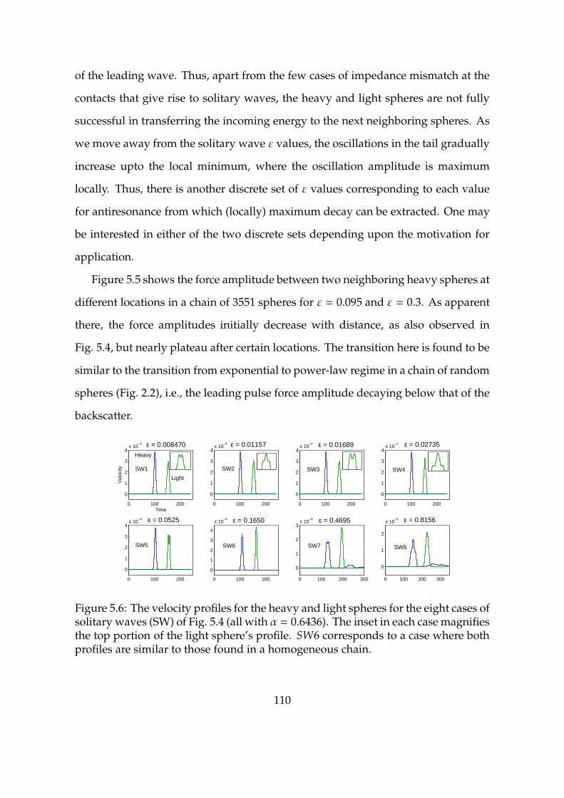
of the leading wave. Thus, apart from the few cases of impedance mismatch at the

contacts that give rise to solitary waves, the heavy and light spheres are not fully

successful in transferring the incoming energy to the next neighboring spheres. As

we move away from the solitary wave ε values, the oscillations in the tail gradually

increase upto the local minimum, where the oscillation amplitude is maximum

locally. Thus, there is another discrete set of ε values corresponding to each value

for antiresonance from which (locally) maximum decay can be extracted. One may

be interested in either of the two discrete sets depending upon the motivation for

application.

Figure 5.5 shows the force amplitude between two neighboring heavy spheres at

different locations in a chain of 3551 spheres for ε = 0.095 and ε = 0.3. As apparent

there, the force amplitudes initially decrease with distance, as also observed in

Fig. 5.4, but nearly plateau after certain locations. The transition here is found to be

similar to the transition from exponential to power-law regime in a chain of random

spheres (Fig. 2.2), i.e., the leading pulse force amplitude decaying below that of the

backscatter.

0 100 200

0

1

2

3

4x 10

−4

Time

Vel

ocity

0 100 200

0

1

2

3

4x 10

−4

0 100 200

0

1

2

3

4x 10

−4

0 100 200

0

1

2

3

4x 10

−4

0 100 200

0

1

2

3

4x 10

−4

0 100 200

0

1

2

3

4

x 10−4

0 100 200 300

0

1

2

3x 10

−4

0 100 200 300

0

1

2

x 10−4

ε = 0.01157 ε = 0.01689 ε = 0.02735

ε = 0.8156ε = 0.4695ε = 0.1650ε = 0.0525

ε = 0.008470

SW2 SW3 SW4

SW5 SW6 SW7 SW8

SW1

Heavy

Light

Figure 5.6: The velocity profiles for the heavy and light spheres for the eight cases ofsolitary waves (SW) of Fig. 5.4 (all with α = 0.6436). The inset in each case magnifiesthe top portion of the light sphere’s profile. SW6 corresponds to a case where bothprofiles are similar to those found in a homogeneous chain.

110

Figure 5.6 illustrates the eight solitary wave cases that were indicated by circular

markers in Fig. 5.4. Each subfigure in Fig. 5.6 shows the velocity histories of a

heavy and a light sphere in a long nonlocal dimer chain. The corresponding ε

value is marked on top of each subfigure, while α = 0.6436 is fixed for all cases.

As observed there, the solitary wave profiles vary depending on the value of ε.

For the cases SW1 − 5, the velocity profiles for the heavy sphere are similar to that

of the homogeneous chain, while those of the light sphere are different with each

case indicating multiple peaks and/or expansions and contractions in certain areas.

However, for the cases SW7 and SW8, the light spheres exhibit a behavior similar to

that of a homogeneous chain while the heavy spheres’ profiles are different, similar

to those of light spheres in SW1 − 5.

In Fig. 5.6, the velocity profiles of the heavy and light spheres corresponding to

ε = 0.165 (SW6) are unique because both the spheres’ responses are similar to that of

a homogeneous chain. Henceforth, we refer to the case SW6 as a single peak solitary

wave (SPSW). In contrast, a case similar to the SPSW case was not found in the local

dimer chain [39]. The present finding indeed constitutes a special case as the system

is inhomogeneous. As we shall discuss later, SPSW cases exist over a wide range

of ε and α values. The width of the SPSW depends on the values of ε and α. In

some cases of the solitary waves, there could also be smaller amplitude waves in

the tail of the solitary waves. For example, SW7− 8 show that the trailing waves are

due to the transient effect and the solitary wave travels without attenuation after

detachment from the tail.

One can compare the SPSW case with the homogeneous chain solitary wave

by extracting the kinetic and potential energy content of the solitary waves and

comparing with the virial theorem [5]. Figure 5.7 shows the history of the total

kinetic and potential energies for the case of SPSW, i.e., ε = 0.165 and α = 0.6436.

The total kinetic (potential) energy is defined as the sum of the kinetic (potential)

111

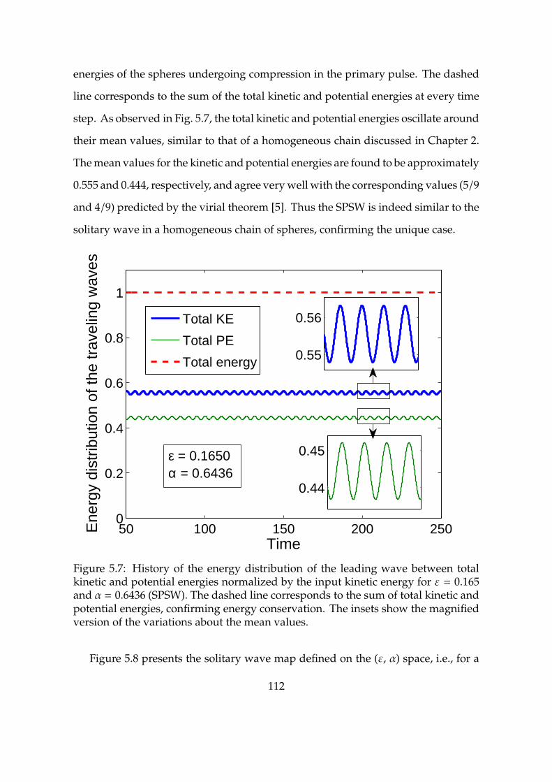
energies of the spheres undergoing compression in the primary pulse. The dashed

line corresponds to the sum of the total kinetic and potential energies at every time

step. As observed in Fig. 5.7, the total kinetic and potential energies oscillate around

their mean values, similar to that of a homogeneous chain discussed in Chapter 2.

The mean values for the kinetic and potential energies are found to be approximately

0.555 and 0.444, respectively, and agree very well with the corresponding values (5/9

and 4/9) predicted by the virial theorem [5]. Thus the SPSW is indeed similar to the

solitary wave in a homogeneous chain of spheres, confirming the unique case.

50 100 150 200 2500

0.2

0.4

0.6

0.8

1

Time

Ene

rgy

dist

ribut

ion

of th

e tr

avel

ing

wav

es

Total KE

Total PE

Total energy 0.55

0.56

Total KE

Total PE

Total energy

0.44

0.45

Total KE

Total PE

Total energy

ε = 0.1650α = 0.6436

Figure 5.7: History of the energy distribution of the leading wave between totalkinetic and potential energies normalized by the input kinetic energy for ε = 0.165and α = 0.6436 (SPSW). The dashed line corresponds to the sum of total kinetic andpotential energies, confirming energy conservation. The insets show the magnifiedversion of the variations about the mean values.

Figure 5.8 presents the solitary wave map defined on the (ε, α) space, i.e., for a

112

wide range of material properties. The stiffness ratio α is chosen in intervals of 0.1

in the range 0.1 to 1.28, which is lower than the maximum value αmax ≈ 1.287 (for

E1/E2 ≪ 1). For each α, wave propagation in a chain of 520 spheres is simulated

with ε ranging from 0.001 to 1 in intervals of 0.001. Then the solitary wave cases

are determined at locations where there is local minimum in force amplitude loss

between sphere number 100 and 500. The case SW6 corresponds to SPSW, as noted

in Fig. 5.6. As evident in Fig. 5.8(a), the eight solitary wave cases discussed earlier

(and labeled SW1 − 8) exist for the range of α studied. Figure 5.8(b) is a magnified

version showing the solitary wave cases SW1 − 5 more clearly as ε → 0. We point

out that the region between the curves give rise to attenuation of the leading wave,

as was observed in Fig. 5.4. Thus, the solitary wave map indicates that there is lot of

flexibility in choosing material combinations for the heavy and light spheres either

to have zero or finite attenuation. Figure 5.8(a) also shows ε and α values for real

material properties to illustrate combinations resulting in either perfect (or near)

solitary wave or a amplitude-decaying response. The numbers labeled next to the

circular markers indicate the material combinations and should be read according to

Table 5.1. The heavy sphere is made of material corresponding to the first digit while

the light sphere’s material is indicated by the second digit of each of the two-digit

labels.

113

0 0.2 0.4 0.6 0.8 10

0.2

0.4

0.6

0.8

1

1.2

1.42125

34

37

41

54

61

65

67

71

ε

αSW7

SW8

SW1−5

SW6

(a)

0 0.02 0.04 0.06 0.08

0

0.2

0.4

0.6

0.8

1

1.2

1.4

ε

α

SW1 SW2 SW3 SW4 SW5

(b)

Figure 5.8: (a) Solitary wave map showing the combinations of ε and α that allowsolitary wave propagation in the bidisperse system. The eight solitary wave casesof Fig. 5.6 are extracted for every α. (b) A magnified version of the map showingthe data for smaller values of ε.

114

Table 5.1: Materials corresponding to the combinations used in Fig. 5.8(a).

Number Material1 Stainless steel2 Delrin3 Polycarbonate4 Aluminum5 Alumina6 PTFE7 Brass

5.3 Analytical investigation

5.3.1 Quasi-continuum approximation

In this section, a continuum approximation of the nonlocal dimer chain based on

a long-wavelength approximation (LWA) is considered. The continuum approxi-

mation employed in this study follows the work by Pnevematikos et al. [64], who

applied the method to nonlinear diatomic chains (see also [23]).

Consider the nondimensional equations of motion (5.4) of the heavy and light

spheres governed by the parameters ε and α. For clarity, let us rewrite the above

equations by denoting the displacement of the ith heavy particle by ui and that of

the light particle by vi as

ui = α[(vi−1 − ui)

3/2 − (ui − vi)3/2

]+

+[(ui−1 − ui)

3/2 − (ui − ui+1)3/2]

(5.6a)

εvi = α[(ui − vi)

3/2 − (vi − ui+1)3/2]. (5.6b)

Defining a = R1 + R2 as the small parameter in the LWA and replacing ui (vi) with

the continuous variable u(x) (v(x)), displacements of the neighboring spheres are

115

defined as [5]

ui±1 = exp

(±2a∂

∂x

)ui (5.7)

= u ± 2aux + 2a2uxx ±4

3a3uxxx +

2

3a4uxxxx + · · · ,

with the light sphere’s displacement (vi) similarly obtained. Substituting Eq. (5.7) in

Eqs. (5.6) results in two coupled partial differential equations (PDEs). To solve these

PDEs, the two displacements ui and vi are decoupled by incorporating the following

condition [64]:

v = σ(u + b1aux + b2a2uxx + b3a3uxxx + b4a4uxxxx + · · ·

), (5.8)

where σ and bi are the unknown coefficients. Due to the ansatz Eq. (5.8), the two

PDEs of Eqs. (5.6) are now only a function of heavy particle’s displacement u. Since

there is only one dependent variable, the parameters σ and bi are determined by

forcing the two PDEs to be equivalent. Similar to the cases discussed in [64] and [23],

there are two possible values for σ, one corresponding to in-phase motion or acoustic

mode (σ = 1) and the other for out-of-phase motion or optical mode (σ = − 1ε ). Here,

we report results for the acoustic mode case (σ = 1), given that the initial impulse

condition for the present study leads to in-phase motion [23].

The parameters bi are then obtained by equating successive orders of the small

parameter a to zero. One obtains the following relations for the parameters b1, b2

116

and b3:

b1 = 1,

b2 =α − 2

√2ε

α(1 + ε),

b3 =2α − 6

√2ε − αε

3α(1 + ε).

(5.9)

Determining the value of b4 is not, however, as straightforward. After the two PDEs

of Eqs. (5.6) are equated, we find that there are several derivative terms at the order

a9/2, where b4 needs to be obtained, while the earlier bi values had just one term at

the corresponding orders of a. The presence of “residual” derivative terms is typical

of problems with second-neighbor interactions [64], which is indeed the case in our

study. The concerned order a9/2 expression is

a9/2[ε(2α3(−1 + ε) + 24αε + 8

√2ε2 −

√2α2(4 + (−10 + ε)

ε))u3

xx + 12αε(− α2(−1 + ε) + 4(−3 + ε)ε +

√2α(2

+ (−5 + ε)ε))uxuxxuxxx + 4α

(− 24ε2 + 2

√2αε(4

+ (−1 + ε)ε) + α2(− 1 + ε − ε2 + 3(1 + ε)3b4

))u2

xu4x

]

= a9/2[P(ε, α)u3

xx +Q(ε, α)uxuxxuxxx + S(b4, ε, α)u2xu4x

]. (5.10)

As apparent in Eq. (5.10), P, Q and S have to be simultaneously zero for the two PDEs

to be identical. We can set S = 0 to obtain b4 as

b4 =1

3α2(1 + ε)3

(α2 − 8

√2αε − α2ε + 24ε2 + 2

√2αε2

+ α2ε2 − 2√

2αε3), (5.11)

but P and Q cannot be equated to zero simultaneously. A similar situation occurs in

the case of original local dimer chain [23], where P = Q, and P = Q = 0 is valid only

117

when ε = 1. In that study, the two functions were neglected, possibly due to the

functions being coefficients of higher-order terms. Thus, a single PDE was obtained

with the assumption that P = Q = 0 and then a traveling wave solution similar

to that of a homogeneous chain was obtained. In the present study, however, we

ask the following question: Is it possible to predict the values (ε, α) for the case of

SPSWs (SW6 in Fig. 5.8(a))? Since P = Q = 0 will yield solitary wave solutions, we

now proceed and compare the solutions of P = 0 and Q = 0 with that of the discrete

data points for SPSWs. The required solutions of P = 0 and Q = 0 are given by

α =

√2ε

(6 − ε +

√52 − 28ε + ε2

)

4 (1 − ε) ,

α =

√2ε (3 − ε)1 − ε ,

(5.12)

respectively. Figure 5.9 shows the α − ε variation as given by Eqs. (5.12) and data

points of SPSWs (SW6) from the map in Fig. 5.8. As evident in Fig. 5.9, the solution

for Q = 0 predicts the numerical data well, while the solution of P = 0 is not very

accurate. At this end, we resort to the technique of introducing an additional term

in the ansatz given in Eq. (5.8), similar to Eq. (3.2) in [64]. This additional term is

guessed based on the residual terms’ derivatives. In our case, P(ε, α)u3xx is chosen as

the residual term that needs to be eliminated, while we enforce Q = 0 to seek solitary

wave solutions. To eliminate the residual term, the additional term in Eq. (5.8) is

taken as b5a4(−ux)−2u3xx, where b5 is given by

b5 =ε

12α3(1 + ε)3

(4√

2α2 + 2α3 − 24αε − 10√

2α2ε − 2α3ε

− 8√

2ε2 +√

2α2ε2). (5.13)

118

0 0.05 0.1 0.15 0.2 0.25 0.30

0.5

1

1.5

2

2.5

ε

α

P=0 imposed

Q=0 imposed

SPSWs numerical

Figure 5.9: Variation of αwith ε comparing the numerical data for SW6 from Fig. 5.8with Eqs. (5.12). The first and the second Eqs. (5.12) correspond to P = 0 (solid line)and Q = 0 (dashed line), respectively.

We now end up with a single PDE in heavy particle’s displacement u given by

utt =3√

2a5/2(−2 + ε)√−uxuxx

−1 + ε

− a9/2(−2 + ε) (−ux)3/2

4√

2(−3 + ε)(−1 + ε)(1 + ε)

((− 3 − 2ε + 4ε2

)u3

xx

+ 4(6 + ε − 5ε2

)uxuxxuxxx − 8

(− 3 + ε + ε2

)u2

xu4x

), (5.14)

with the same order derivative terms as in the homogeneous chain’s PDE [5] but

with different coefficients. Rescaling the time variable (t) as

τ = t

√3√

2a5/2(2 − ε)/(1 − ε). (5.15)

119

We can now obtain exact periodic solutions for traveling waves with the transforma-

tion ξ = x−Vτ, where V is the wave speed. The new definition transforms the PDE

of Eq. (5.14) into an ODE in the first derivative of u (uξ) (see [23] for intermediate

steps). We find the final solution as

uξ = B(ε)cos4 (b(ε)ξ) , (5.16)

where the amplitude of the wave B(ε) and the characteristic spatial wavelength w(ε)

as a function of b(ε) are given by

B(ε) =9V4(15 − 2ε − 8ε2)2

4(12 − ε − 7ε2)2, (5.17)

w(ε) =π

b(ε)=√

2aπ

√15 − 2ε − 8ε2

3 + 2ε − ε2, (5.18)

respectively.

Figure 5.10(a) shows the variation of the normalized spatial wavelength (w/a)

with ε, as given by Eq. (5.18). We note that ε = 1 exactly recovers the 1D homo-

geneous chain solution of Nesterenko [5], which is about five particle diameters.

Figure 5.10(b) shows the velocity profiles from simulations for ε = 0.165 and ε = 0.7

(markers in Fig. 5.10(a)). Thus the spatial wavelengths from simulations for ε = 0.165

and ε = 0.7 are found to be about 10 and 8 particle diameters, respectively, showing

a very good agreement with the analytical prediction of Fig. 5.10(a).

120

0 0.2 0.4 0.6 0.8 14

5

6

7

8

9

10

ε

Wav

e w

idth

(w

/a)

(a)

40 42 44 46 48 50 52 540

1

2

3

4

x 10−6

Sphere number

Vel

ocity

34 36 38 40 42 44 460

0.5

1

1.5

2

x 10−5

(b)

Figure 5.10: (a) Normalized spatial wavelength (w/a) as a function of ε from theanalytical solution (5.18). (b) Velocity profiles (illustrating spatial wavelength) forthe two cases of εmarked by symbols in Fig. 5.10(a) (ε = 0.165 and ε = 0.7), showinga good comparison with the analytical solution.

121

By employing the solution for strain variable (Eq. (5.16)), one can also obtain

the wave speed as a function of its force amplitude [2]. Figure 5.11 compares the

wave speed-force amplitude dependence for ε = 0.165 with that of the simulations.

A reasonable comparison (with an error of about 9.5%) is obtained with the error

arising from the quasi-continuum approximation and the fact that the force ampli-

tude varies as Fm ∝ V6, i.e., the error is more pronounced since the phase velocity is

raised to the power six.

0 0.5 1 1.5 2 2.5 3

x 10−3

0.5

0.6

0.7

0.8

0.9

1

1.1

Force amplitude

Wav

e sp

eed

SimulationsAnalytical

Figure 5.11: Nondimensional wave speed as a function of the force amplitudecomparing the simulation results with the analytical solution from (5.16).

5.3.2 Asymptotic analysis

In the previous section, the set of values of ε and α for the case of SPSWs was

predicted by using a quasi-continuum approach. In this section, the objective is to

122

predict the solitary waves over a wider range of ε andαwith the aid of an asymptotic

method [65].

Consider the normalized equations of motion in Eq. (5.4), where ε is considered

small in the following analysis, i.e., 0 < ε ≪ 1, while there is no restriction on

α. As discussed in [65, 39], the main principle behind the asymptotic method

adopted hereafter is the separation of time scale in the limit of small ε. Thus, for

the primary (solitary) wave propagation, we can write the heavy and light spheres’

displacements (ui and ui+1) with the following asymptotic expansions:

ui = ui0(t0) + ελui1(t1) + · · · ,

ui+1 = u(i+1)0(t0) + εγu(i+1)1(t1) + · · · ,(5.19)

where the separated time scales are t0 = τ and t1 = εβt0 and λ, γ and β are the

unknowns to be determined. We now substitute Eq. (5.19) in Eq. (5.4) along with

the two time scales, and then expand the relevant terms in power series as ε→ 0 to

obtain, for the heavy sphere,

ui0 + ελ+2βu

′′

i1 =α[(

u(i−1)0 − ui0

)3/2−

(ui0 − u(i+1)0

)3/2]

+(u(i−2)0 − ui0

)3/2−

(ui0 − u(i+2)0

)3/2

+ (3/2)α(u(i−1)0 − ui0

)1/2 (εγu(i−1)1 − ελui1

)

− (3/2)α(ui0 − u(i+1)0

)1/2 (ελui1 − εγu(i+1)1

)

+ (3/2)ελ(u(i−2)0 − ui0

)1/2 (u(i−2)1 − ui1

)

− (3/2)ελ(ui0 − u(i+2)0

)1/2 (ui1 − u(i+2)1

)

+O(∥∥∥ελui1 − εγu(i+1)1

∥∥∥2),

(5.20)

123

while the light sphere’s equation expands to

ε(u(i+1)0 + ε

γ+2βu′′(i+1)1

)=

α[(

ui0 − u(i+1)0

)3/2−

(u(i+1)0 − u(i+2)0

)3/2

+ (3/2)(ui0 − u(i+1)0

)1/2 (ελui1 − εγu(i+1)1

)

− (3/2)(u(i+1)0 − u(i+2)0

)1/2 (εγu(i+1)1 − ελu(i+2)1

)

+O(∥∥∥ελui1 − εγu(i+1)1

∥∥∥2)].

(5.21)

In Eqs. (5.20) and (5.21), overdots and primes correspond to differentiation with

respect to the two times scales, t0 and t1, respectively. One can now compare different

terms at each order to obtain the unknown parameters λ, γ and β. From the left

hand side of Eq. (5.20), we can choose λ + 2β = 1 for the first-order approximation,

which allows us to choose either λ = 1 or γ = 1 or λ = γ = 1 from the right hand

side of the equation. Since β cannot be zero (β = 0 implies no separation of time

scales), we choose γ = 1. Equation (5.21) now implies γ + 2β = 0, which yields

β = −1/2 and λ = 2. Thus, t1 = ε−1/2t0 and Eqs. (5.20) and (5.21) have errors of order

∥∥∥ε2ui1 − εu(i+1)1

∥∥∥2.

We now proceed to obtain the approximations at various orders of Eqs. (5.20) and

(5.21) essentially yielding the slow (zeroth-order approximation) and fast dynamics

(first-order approximation) components of the above equations. The zeroth-order

approximations for heavy and light spheres are obtained as

ui0 =α[(

u(i−1)0 − ui0

)3/2−

(ui0 − u(i+1)0

)3/2]

+(u(i−2)0 − ui0

)3/2−

(ui0 − u(i+2)0

)3/2,

u(i+1)0 =ui0 + u(i+2)0

2,

(5.22)

respectively. Thus the slow dynamics of the light sphere (indicated by its depen-

124

dence on t0 alone) is simply the average of the slow dynamics of its neighboring

heavy spheres, similar to the local dimer chain [39]. The slow dynamics of a heavy

sphere is more complicated due to the presence of nonlocal interactions. However,

one can simplify the first Eq. (5.22) further by substituting the response of the light

spheres from second Eq. (5.22):

ui0 =

(1 +

α

23/2

) [(u(i−2)0 − ui0

)3/2−

(ui0 − u(i+2)0

)3/2],

u(i+1)0 =ui0 + u(i+2)0

2.

(5.23)

The slow dynamics of the heavy sphere (first Eq. (5.23)) now solely depends on

the nonlocal interactions with its nearest heavy spheres, which is equivalent to

the response of a homogeneous chain of heavy spheres. We observe that the first

Eq. (5.23) has an explicit dependence on α while it is a constant in the local dimer

chain [39].

The dynamic response of a homogeneous chain of spheres is basically a solitary

wave [5]. Thus, the zeroth-order solution for both heavy and light spheres does

not lead to formation of any ”tail”. In the open literature, there are a number of

analytical approximations [5, 3] which are applicable to the first Eq. (5.23). We

choose the solution by Sen et al. [6], which has been shown to be more accurate than

the solution by Nesterenko [5]. The displacement of the solitary wave is described

in terms of the hyperbolic tangent function as [3]

S(z) =A + (A/2)[tanh

(C1(z/T) + C3(z/T)3

+ C5(z/T)5)/2

− 1

],

C1 =2.39536, C3 = 0.268529, C5 = 0.0061347,(5.24)

where A and T are the amplitude of the solitary wave and time taken by the solitary

wave to reach maximum amplitude between two neighboring spheres, respectively.

In order to obtain the displacements of the individual spheres in the system (5.23),

125

the following transformations are employed:

ui0(t0) =Si(kt0), k = (1 + α/23/2)1/2,

Si(kt0) =S[k(t0 − iT)].(5.25)

By employing the above solution for the slow dynamics of the heavy spheres, the

slow dynamics of the light spheres can be written as

u(i+1)0 =Si(kt0) + Si+2(kt0)

2. (5.26)

Since the zeroth-order solution does not have any trailing waves for any ε and

α, higher-order approximation is necessary to find the discrete set of values of ε and

α for which the tail goes to zero, i.e., for the formation of solitary waves. We now

proceed to the first-order approximation (O(ε)) in Eqs. (5.20) and (5.21) to obtain the

following relations for the fast dynamics component of the heavy and light spheres:

u′′i1 =(3/2)α(Si−1(kt0) − Si(kt0))1/2(u(i−1)1(t1)

)

+ (3/2)α(Si(kt0) − Si+1(kt0))1/2(u(i+1)1(t1)

),

u′′(i+1)1(t1) +Ω2i+1(t0)u(i+1)1(t1) = fi+1(t0).

(5.27)

In second Eq. (5.27),Ω2 is the natural frequency and f is the force excitation, which

are functions of the zeroth-order (slow) responses of the spheres as given by

Ω2i+1(t0) =3α

(ui0(t0) − u(i+2)0(t0)

2

)1/2

,

fi+1(t0) = − si+1(kt0).

(5.28)

Furthermore, we observe that Eqs. (5.27) are linear oscillators, where the second

Eq. (5.27) is solely a function of light sphere’s displacement, i.e., it is uncoupled.

126

The uncoupled linear oscillator is then numerically integrated to find the cases for

which solitary waves are formed. The second Eq. (5.27) is sufficient because a zero

tail in the light sphere’s fast response implies a zero tail in the heavy sphere’s fast

response.

We direct the reader to Ref. [39] for a detailed discussion on the relevant condi-

tions for the formation of localized solitary waves with compact support. In essence,

the necessary and sufficient conditions for the generation of these specific solitary

waves respectively are

u(i+1)1(t1 = 0) = 0,

limt1→+∞

u′(i+1)1(t1) = 0,(5.29)

where the time axis is shifted such that the reference time τ = 0. Then the differential

equation to be solved to determine the values of ε (for a givenα) that satisfy Eq. (5.29)

is given by

u′′(i+1)1(t0) +Ω2

i+1(t0)

εu(i+1)1(t0) =

fi+1(t0)

ε. (5.30)

Equation (5.30) is just another version of the second Eq. (5.27), with the fast

time scale (t1) written in terms of the slow time scale (t0). Equation (5.30) is solved

numerically by iterating over various values of 0 < ε ≤ 1. Figure 5.12 shows the

variation of the displacement u(i+1)1 at t0 = 0 as a function of ε for α = 0.6436. We

note the oscillatory nature of the displacement leading to the existence of countable

infinity of discrete values of ε that have u(i+1)1(0) = 0, i.e., solitary waves. For ε values

close to zero, we need a much finer spacing between any two values to obtain more

accurate results. The circular markers correspond to the six solitary wave cases

SW1−6 in Fig. 5.6 which were shown for the same α = 0.6436. Thus, the asymptotic

method fails to predict solitary waves beyond SW6. The primary reason for this

127

limited application is that the fast dynamics is no longer in the light sphere but is

shifted to the heavy sphere, as shown in the velocity profiles for SW7 and SW8 in

Fig. 5.6.

10−4

10−3

10−2

10−1

100

−0.5

0

0.5

ε

Dis

plac

emen

t (fa

st d

ynam

ics)

Displacement

Solitary wave cases

Figure 5.12: Fast dynamics displacement component of the light sphere at t0 = 0 asa function of ε (on log scale). The solitary wave cases SW1 − 6 (Fig. 5.6) are markedwith circles.

Figure 5.13 shows the history of fast dynamics component of the displacement

(u(i+1)1) and the total velocity (ui+1) of the light sphere for ε = 0.01692 and α = 0.6436.

As the displacement is anti-symmetric (u(i+1)1(0) = 0) and the velocity is decaying to

zero after a certain time, this case corresponds to the solitary wave SW3 in Fig. 5.6.

We can also observe that the velocity profile is captured well by the asymptotic

method. The number of peaks (or valleys) in the displacement profile indicates the

number of ”humps” in the traveling wave. Therefore, there are four humps for

128

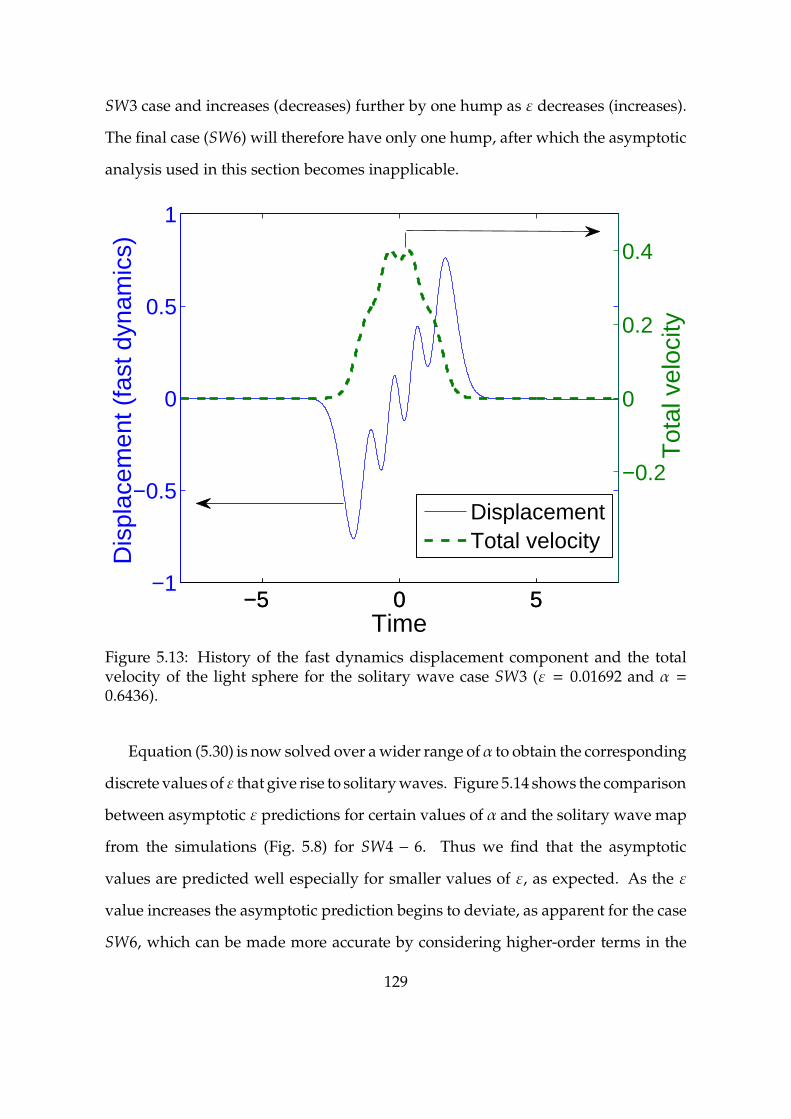
SW3 case and increases (decreases) further by one hump as ε decreases (increases).

The final case (SW6) will therefore have only one hump, after which the asymptotic

analysis used in this section becomes inapplicable.

−5 0 5−1

−0.5

0

0.5

1

Dis

plac

emen

t (fa

st d

ynam

ics)

Time

−5 0 5

−0.2

0

0.2

0.4

Tot

al v

eloc

ity

DisplacementTotal velocity

Figure 5.13: History of the fast dynamics displacement component and the totalvelocity of the light sphere for the solitary wave case SW3 (ε = 0.01692 and α =0.6436).

Equation (5.30) is now solved over a wider range of α to obtain the corresponding

discrete values of ε that give rise to solitary waves. Figure 5.14 shows the comparison

between asymptotic ε predictions for certain values of α and the solitary wave map

from the simulations (Fig. 5.8) for SW4 − 6. Thus we find that the asymptotic

values are predicted well especially for smaller values of ε, as expected. As the ε

value increases the asymptotic prediction begins to deviate, as apparent for the case

SW6, which can be made more accurate by considering higher-order terms in the

129

asymptotic expansions (5.19). We again emphasize that the SW6 case is the final

case predicted by the aforementioned asymptotic analysis.

0 0.05 0.1 0.15 0.2 0.25 0.30

0.2

0.4

0.6

0.8

1

1.2

ε

α

Simulations

Asymptotics

SW4 SW5

SW6

Figure 5.14: α-ε variation for the solitary wave cases SW4−6 comparing the asymp-totic solution (circles) with the numerical simulation (solid lines) (Fig. 5.8). SW6corresponds to the SPSW case.

5.4 Conclusions

A numerical investigation was undertaken to study plane wave propagation in a

2D square packing system of spherical particles with intruders at interstitial loca-

tions. The granular system was considered to be periodic in the lateral direction and

semi-infinite in the direction of propagation. Nondimensionalizing the system of

equations demonstrated two key parameters governing the dynamics of the granu-

130

lar system: the mass ratio ε and the stiffness ratioα. An equivalent 1D granular chain

was proposed based on the periodicity of the closed-packed system and the planar

impact loading. The equivalent granular chain, termed nonlocal dimer chain, differs

from the original dimer chain due to the presence of additional nonlocal interactions

between nearest larger spheres. The 1D equivalence was verified by comparing the

numerical results of the 1D and 2D systems. Further investigation of the nonlocal

dimer chain revealed the existence of a new family of solitary waves for discrete

combinations of ε and α. The solitary waves were found to propagate with different

profiles depending on the nondimensional parameters α and ε. Furthermore, an

unique case of a solitary wave where the profile is similar to that of a homogeneous

chain was reported in the present inhomogeneous system. A systematic procedure

was performed to generate a solitary wave map of combinations of ε and α en-

compassing some of the solitary wave cases. Finally, a couple of analytical studies

were conducted to predict the solitary wave cases, particularly the case similar to

the homogeneous solitary wave. By employing a quasi-continuum approximation,

the discrete system of partial differential equations was reduced to a single ordinary

differential equation and a solitary wave solution was obtained. Wave width and

wave speed-force amplitude dependence were compared with the analytical solu-

tion and showed a good agreement. In another approach, an asymptotic analysis

was performed to predict the discrete values of material combinations for the exis-

tence of solitary waves in the limit of ε → 0. The asymptotics also demonstrated a

very good agreement with the solitary wave map generated from the simulations.

131

Chapter 6

Embedded granular systems

Due to the inherently nonlinear properties of the inter-particle contact, granular

chains have unique wave propagation properties that are increasingly being con-

sidered for impact protection and wave tailoring applications. However, most of

the work so far has focused on ‘laboratory granular systems’ in the absence of a

container or matrix material. However, the granular chains need to be embedded

in a matrix or contained if these systems are to be deployed in engineering applica-

tions. A computational analysis of this new class of granular chain-matrix material

system is the topic of this chapter. We undertake a preliminary study to investigate

the bending response of a linear elastic beam with granular chains embedded in

an ordered manner. A key motivation comes from the unique flexibility of gran-

ular chains with regard to response of the spherical particles under compression

or tension. This ‘unusual’ response can be visualized by considering the granular

chains as nonlinear ‘fibers’ with zero stiffness under tension whereas they follow

the Hertzian law under compression. Thus, depending on the presence or absence

of the contact forces, spheres or the surrounding matrix may play a dominant role

in the bending response. The no-tension condition thus yields a unique kind of

bending behavior where some of the chains are under compression while some are

in tension depending on their locations with respect to the neutral axis.

Our previous studies on the effect of randomness on wave propagation in granu-

lar systems have shown that the energy carried by the wavefront decays very quickly

due to backscattering, and thus emphasis will be placed on avoiding randomness

132

in the embedded granular system. Some of the ways the spheres can be packed

together is by filling matrix material in between the spheres or drilling holes in a

matrix to accommodate granular networks. Experiments such as dynamic impact of

square or hexagonal packing of spheres in a matrix, energy transfer between two or

more chains in a matrix and numerically extracting a quasi-static force-displacement

law at the sphere-matrix interface have demonstrated some challenges in manufac-

turing and testing the “infused” configuration, thus the focus of our studies will be

on the “drilled” configuration.

The remainder of the chapter is organized as follows: Section 6.1 defines the

problem and describes the numerical setup. In Sec. 6.2,we present the finite element

formulation for the embedded granular system is presented. Section 6.3 explains

the algorithm used in current study. Sections 6.4 and 6.5 verify the finite element

program and perform convergence studies, respectively. Section 6.6 summarizes

the results of dynamic studies of embedded granular systems. Precompression in

the granular chains is also expected to play a role in the bending response because

it directly affects the amplitude of vibration. In Sec. 6.6, we also perform studies

to investigate the effect of precompression on the bending behavior particularly at

resonance.

6.1 Problem description and numerical setup

Consider a beam made of a linear elastic homogeneous material and fixed at both

ends. In the axial direction of the beam, i.e., parallel to the neutral axis, one or more

homogeneous granular chains are inserted by drilling holes into the beam. The

granular chains are assumed to extend from the left to right end of the beam. Figure

6.1 shows an example where one chain of spheres is inserted into a beam fixed at

both ends. The beam is subjected to a point load at the center of the top edge.

133

Figure 6.1: A granular chain embedded at the center of a linear elastic beam. Theloading is applied at the center of the beam.

A finite element solver is written in MATLAB® to simulate the static and dy-

namic behavior of beams embedded with granular chains. The granular chains are

approximated as continuum bar elements where a nonlinear force-displacement re-

lationship is derived. Then we seek the tangent stiffness matrix which is employed

in the Newton-Raphson technique. Newmark method is used for numerical time

integration. In our studies, the material properties for the linear elastic beam and

spheres are fixed corresponding to epoxy and steel, respectively. Epoxy (steel) prop-

erties are taken as: Young’s modulus E = 2.3 GPa (200 GPa), Poisson’s ratio ν = 0.37

(0.3) and density ρ = 1200 kg/m3 (7850 kg/m3). The dimensions of the beam are

given by 0.5 m by 0.01 m by 0.01 m unless otherwise mentioned. The displacement

(d) is normalized by the center displacement amplitude for a static loading on a

beam fixed at both ends and time (t) is normalized by the angular frequency of the

applied loading (ω), i.e.,

d =d(

FmaxL3

192EI

) , (6.1)

t = tω, (6.2)

where L is the length of the beam and I is the area moment of inertia of the beam

cross-section. We consider a harmonic loading of amplitude Fmax = 0.01 N to study

the overall bending response of the beam.

134

6.2 Finite element formulation

The linear elastic beam is modeled as a 2D plane-stress problem discretized into four-

node quadrilateral elements. The equations of linear elasticity and its finite element

formulation for quadrilateral elements are not presented here but the interested

reader can obtain the formulation in any introductory text on the finite element

method [66, 67]. As alluded to earlier, we approximate one or more spheres in a

granular chain as a continuum bar element. Thus the granular chain is replaced by

a series of bar elements. We first obtain a constitutive relation for the bar element

which is then combined with that of the quadrilateral elements.

Figure 6.2: A chain of spheres discretized into a number of bar elements with eachbar element consisting of N spheres.

Consider a single chain of spheres as shown in Fig. 6.2. Let us assume that there

are N number of spheres in a bar element. Here, we note that the centers of the

first and Nth spheres represent the nodes of the bar element. Thus the length of the

element is l = (N−1)D, where D is the diameter of a sphere. Consider a compressive

force F applied at each end of the element. The total deformation ∆t in the element

can be written as

∆t = (N − 1)∆, (6.3)

where∆ is the deformation at a single contact. The deformation at a contact between

two spheres can be related to the force applied by using the Hertzian law described

in the previous chapters. Thus, ∆t translates to

∆t = (N − 1)(

F

K

)3/2

, (6.4)

135

where K = 2Es/(3(1 − ν2s ))√

R/2 is the contact stiffness and R is the radius of a

sphere. The strain in the chain of N spheres can now be approximately determined

by dividing the total deformation of Eq. (6.4) by the length of the element. Thus, we

obtain

ε =∆t

l, (6.5)

=1

D

(F

K

)2/3

. (6.6)

Now we translate the above definitions to bar element variables shown in Fig. 6.3.

The forces at ends of the bar element are related to the compressive force F by

F1 = −F2 = F. The strain variable as a function of the displacements u1 and u2 is

ε =u2 − u1

l. (6.7)

We now recall that there is no tensile force between the spheres, i.e., there is no

contact force if the spheres separate. Combining Eqs. (6.5) and (6.7), the forces F1

and F2 of the bar element are now written as

F1 = −F2 = F =

K(N−1)3/2 (u1 − u2)3/2 if ε < 0,

0 otherwise.

Figure 6.3: Bar element illustrating the nodal displacements and forces.

The bar element’s nonlinear force-displacement relation derived above is com-

bined with the linear constitutive stress-strain relations of the quadrilateral elements

136

of the beam. The force-displacement relations for the bar and quadrilateral elements,

and their tangential stiffness matrices are given in Appendix A.

6.3 Implementation

We solve for the displacements at each node of the beam after assembling the

Eqs. (A.1) and (A.2). The equations are evidently nonlinear as the force-displacement

relations for the bar elements are nonlinear. At each Newton-Raphson iteration we

determine the active bar elements (ε < 0) based on the displacements of the previous

iteration (or initial displacements for the first iteration). The tangential stiffness

matrix is then calculated for the active bar elements. The internal force vector is

then computed by adding the contribution of the bar elements at corresponding

nodes to the contribution of the beam alone (quadrilateral elements). The Newmark

time stepping scheme defines the modified stiffness matrix and force vector, which is

then used to determine the displacement increments in a Newton-Raphson iteration.

Convergence is monitored by comparing the relative norm of the displacement

solution with a tolerance value of 10−3. Finally, acceleration and velocity vectors are

updated by using the converged values of displacement. The algorithm used for

finding the converged solution for displacements is summarized in Algorithm 1. A

more detailed explanation of the algorithm is given in Appendix A.

137

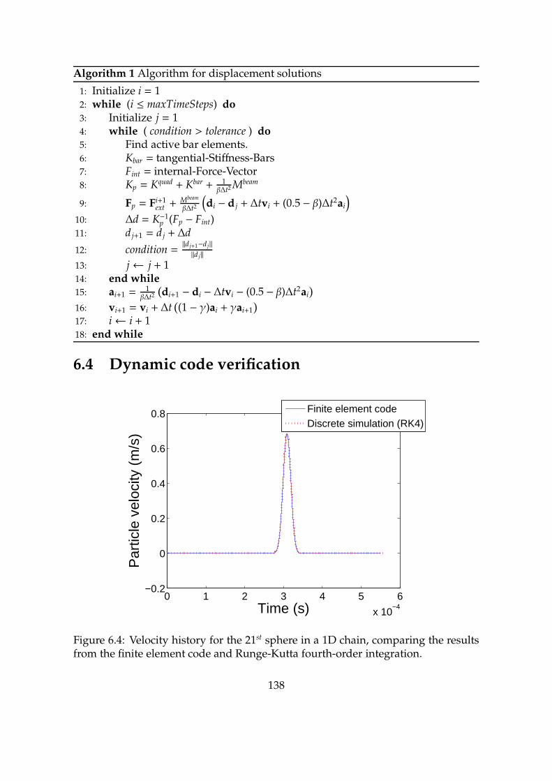
Algorithm 1 Algorithm for displacement solutions

1: Initialize i = 12: while (i ≤ maxTimeSteps) do3: Initialize j = 14: while ( condition > tolerance ) do5: Find active bar elements.6: Kbar = tangential-Stiffness-Bars7: Fint = internal-Force-Vector8: Kp = Kquad + Kbar + 1

β∆t2 Mbeam

9: Fp = Fi+1ext +

Mbeam

β∆t2

(di − d j + ∆tvi + (0.5 − β)∆t2ai

)

10: ∆d = K−1p (Fp − Fint)

11: d j+1 = d j + ∆d

12: condition =‖d j+1−d j‖‖d j‖

13: j← j + 114: end while15: ai+1 =

1β∆t2

(di+1 − di − ∆tvi − (0.5 − β)∆t2ai

)

16: vi+1 = vi + ∆t((1 − γ)ai + γai+1

)

17: i← i + 118: end while

6.4 Dynamic code verification

0 1 2 3 4 5 6

x 10−4

−0.2

0

0.2

0.4

0.6

0.8

Time (s)

Par

ticle

vel

ocity

(m

/s)

Finite element codeDiscrete simulation (RK4)

Figure 6.4: Velocity history for the 21st sphere in a 1D chain, comparing the resultsfrom the finite element code and Runge-Kutta fourth-order integration.

138

In this section, we verify the MATLAB program for dynamic nonlinear finite ele-

ment analysis of embedded granular systems with other sources. First, the nonlinear

bar elements representing a granular chain are considered separately for verifica-

tion purposes. We compare the finite element program results with a Runge-Kutta

fourth-order discrete solver which has been previously verified in Chapter 2. Con-

sider a chain of 40 steel spheres, with the first sphere given an initial velocity of 1

m/s. We choose N = 2, and thus we have 39 bar elements as each element will have

an equivalent of one sphere. The same initial condition is specified to the left node

of the first bar element. Figure 6.4 shows the velocity history for the 21st sphere in

the granular chain and the corresponding node in the series of 1D bar elements. As

evident there, the two results compare very well, thus verifying the finite element

formulation for the granular chain.

0 0.1 0.2 0.3 0.4 0.5 0.6 0.7−5

0

5x 10

−3

Time

Tip

dis

plac

emen

t

Dynamic solverAbaqus

Figure 6.5: Normalized tip displacement history for harmonic type of loading,comparing Abaqus and MATLAB code results.

The finite element code for a linear elastic beam comprising of four-node quadri-

lateral elements is verified using AbaqusTM. We define the following example to

139

compare the two results. Consider a cantilever beam fixed at the left end and made

of epoxy. In this case, the dimensions of the beam are given by 0.4 m by 0.05 m by

0.01 m. As before, a harmonic loading is applied at the right end of the beam and

the mesh size is chosen as 20 by 10 elements. Figure 6.5 shows the tip displacement

history over a certain interval of time comparing both Abaqus and the finite element

(MATLAB) code results. As apparent there, the displacement profiles agree very

well. Figure 6.6 then compares the velocity histories for the two cases in the same

interval of time, again showing very good agreement.

0 0.1 0.2 0.3 0.4 0.5 0.6 0.7

−0.1

−0.05

0

0.05

0.1

0.15

Time

Tip

vel

ocity

Dynamic solverAbaqus

Figure 6.6: Tip velocity (m/s) history for harmonic type of loading, comparingAbaqus and MATLAB code results.

6.5 Convergence studies

In this section, we perform convergence studies with respect to the number of

elements in the longitudinal (x) and transverse (y) directions and the time step used

in the Newmark method. The convergence studies are conducted for the linear case,

140

where a harmonic loading of frequency 25 Hz is applied to a beam fixed at both ends.

The dimensions and material properties of the beam are same as that mentioned in

Sec. 6.1. First, the number of elements in the x direction is kept constant at 20 while

that in the y direction is varied. Figure 6.7 shows the displacement history for three

cases of discretization. Thus, based on the results for 4 and 6 y-elements, we choose

the latter as the converged number in the y direction.

0 5 10 15 20−0.5

0

0.5

Time

Dis

plac

emen

t

20x220x420x6

Figure 6.7: Normalized center displacement history showing convergence withrespect to number of elements in the y direction. Normalization factors are shownin Sec. 6.1.

Then, we fix the number of y elements as 6 and vary x elements from 20 to 120.

Figure 6.8 shows the center displacement history for five cases of mesh size. We

can therefore observe that there is substantial variation in the initial three cases, i.e.,

x-elements of 20, 40 and 60. The number of x-elements is expected to play a bigger

role than the y-elements since we are solving a beam bending problem. We ignore

small deviations and choose number of x-elements equal to 100 as the converged

value.

141

Finally, we consider the time step used in the Newmark method for marching.

Since the run time of a simulation depends on the time step, the convergence study

would help us choose an optimum value. Figure 6.9 shows the center displacement

history for three values of time step, ∆t = 5 × 10−5, 1 × 10−4 and 2 × 10−4 seconds.

As evident there, the results are not very sensitive to the time step for the chosen

applied frequency and time interval. As also indicated by the inset of Fig. 6.9, we

choose ∆t = 1 × 10−4 seconds as an optimum value. Although the above studies

were performed for the linear case, we found the convergence to be valid for the

nonlinear case as well.

0 5 10 15 20

−2

−1

0

1

2

Time

Dis

plac

emen

t

20x640x660x6100x6120x6

Figure 6.8: Normalized center displacement history showing convergence withrespect to number of elements in the x direction.

142

0 20 40 60 80

−2

−1.5

−1

−0.5

0

0.5

1

1.5

2

Time

Dis

plac

emen

t

∆t = 5x10−5 s

∆t = 1x10−4 s

∆t = 2x10−4 s

Figure 6.9: Normalized center displacement history showing convergence withrespect to time step ∆t. Inset shows the magnified version of part of the result forclarity.

6.6 Results: dynamic loading

6.6.1 Linear elastic beam

Consider a linear elastic beam made of epoxy and fixed at both ends. As before, a

harmonic loading of a certain frequency is applied at the center of the beam. Figure

6.10 shows the center displacement amplitude as a function of the loading frequency.

We observe that at a certain frequency, the displacement amplitude reaches a peak

value which corresponds to the familiar point of resonance. The loading frequency

is taken in intervals of 0.1 Hz near the peak value and 1 Hz elsewhere. Since the run

time of the simulation is finite (2 seconds), the displacement amplitude at resonance

is finite but theoretically the value tends to infinity. A theoretical prediction for the

143

first natural frequency can be obtained from the beam equation as

ω1 = 2π f =

√EI

ρAL4, (6.8)

where A is the cross-section area. The dashed line in Fig. 6.10 corresponds to Eq. (6.8).

Now consider the point of resonance where the frequency is 59.52 Hz. Figure 6.11

shows the center displacement history at the resonance frequency and as expected

the displacement amplitude grows linearly with time. Therefore, in absence of

damping, the displacement amplitude tends to infinity for a linear elastic beam.

50 55 60 65 700

50

100

150

200

250

Applied frequency (Hz)

Dis

plac

emen

t am

plitu

de

Theoretical

Figure 6.10: Normalized center displacement amplitude as a function of appliedfrequency for the linear elastic beam without granular chains with the dashed linecorresponding to the theoretical prediction for resonance frequency.

144

0 100 200 300 400 500 600−300

−200

−100

0

100

200

300

Time

Dis

plac

emen

t

Figure 6.11: Normalized center displacement history for the linear elastic beamwithout granular chains, showing indefinite growth in amplitude.

6.6.2 Embedded granular system

We now embed a granular chain at the top of the beam, i.e., the line of sphere centers

corresponds to the top edge of the beam. The main idea is to embed the chain farthest

from the neutral axis to derive maximum advantage during bending. The spheres

are made of steel and of diameter 4 mm, resulting in N = 2.25. Similar to Sec. 6.6.1,

a harmonic loading is applied at the center of the beam at different frequencies. The

run time of each simulation is 6 seconds. Figure 6.12 shows the variation of center

displacement amplitude with the applied frequency ranging from 40-60 Hz. The

frequency is applied in intervals of 0.5 Hz except near the peak value, where the

interval gap is either 0.05 Hz or 0.01 Hz. Thus, as in the beam case, the displacement

amplitude reaches a peak value at a particular frequency.

145

40 45 50 55 600

50

100

150

200

250

Applied frequency (Hz)

Dis

plac

emen

t am

plitu

de

A1

A3

A2

Figure 6.12: Normalized center displacement amplitude as a function of appliedfrequency for the embedded granular system with no precompression.

However, there are some key differences in the embedded system’s response. The

variation of the displacement amplitude in Fig. 6.10 is symmetric with respect to

the resonance frequency. In Fig. 6.12, however, the displacement amplitude drops

sharply on the right side of the peak value. The sharp drop suggests similarity

to the jump phenomenon observed in forced oscillations of nonlinear systems [68].

Although the exact reason is yet to be ascertained, the displacement histories at/near

the peak location might provide us with more information. Another difference is

that the peak displacement amplitude is much lower than that in Fig. 6.10 (which

should be multiplied by a factor of 3 since the run time for the linear case was 2

seconds). However, we should note that the masses of the two systems are not

equal since the present formulation does not remove the corresponding beam mass

to embed the spheres.

146

0 500 1000 1500 2000 2500 3000 3500−300

−200

−100

0

100

200

300

Time

Dis

plac

emen

t

Figure 6.13: Normalized center displacement history for the embedded granularsystem with no precompression at frequency 49.34 Hz corresponding to the peakdisplacement in Fig. 6.12.

Figures 6.13 and 6.14 show the displacement histories at frequencies 49.34 Hz

and 49.35 Hz, respectively. In Fig. 6.12, the two frequencies correspond to the

peak displacement amplitude (labeled ‘A1’) and the next data point after the sharp

decrease (labeled ‘A3’), respectively. Firstly, Fig. 6.13 reveals that the displacement

actually reaches a maximum value at a certain instant and the cycle is repeated

similar to beats. Here, we have demonstrated one of the primary results of this study

where the displacement amplitude near the point of resonance, although still of high

magnitude, reaches a finite value, unlike a linear elastic beam (Fig. 6.11). Figure 6.13

also shows that the variation is highly nonlinear, arising from the Hertzian contact

law. The data point labeled ‘A2’ in Fig. 6.12 has a displacement profile similar to

that of the data point labeled ‘A1’.

147

0 500 1000 1500 2000 2500 3000 3500−80

−60

−40

−20

0

20

40

60

80

Time

Dis

plac

emen

t

Figure 6.14: Normalized center displacement history for the embedded granularsystem with no precompression at frequency 49.35 Hz corresponding to the pointright of the peak value in Fig. 6.12.

At the right of the peak value, however, the displacement history is very different

from that of the peak value. The displacement profile in Fig. 6.14 is similar to

the usual beat phenomenon that we also observe in linear elastic beams near the

resonance frequency. As also observed in Fig. 6.14, the displacement amplitude is

about three times lower, the beat frequency is around two times higher than that

of the variation at the peak value (Fig. 6.13). Thus we observe a drastic change

although the change in applied frequency is just 0.01 Hz.

Let us now suppose that the spheres are precompressed at inter-particle contacts,

holding the two ends of the chain through the built-in ends of the embedded system.

Let us define a nondimensional parameter ∆ = δ/R, where δ is the amount or level

of precompression at each contact and R is the radius of a sphere. Figure 6.15 shows

the variation of the center displacement amplitude with frequency of loading for

different levels of precompression ranging from ∆ = 0 to 5 × 10−4 which, for steel

148

beads of diameter 4 mm corresponds to a precompression level of 0 to 4.63 N. We

earlier considered the case of ∆ = 0 in Fig. 6.12. As evident in Fig. 6.15, the peak dis-

placement amplitude and the frequency at which it occurs change with the applied

precompression level. The frequency at which the displacement amplitude peaks

shows a monotonic increase with ∆ while the displacement amplitude increases

upto ∆ = 1 × 10−4 and then decreases. Furthermore, there is no particular trend

in our results as to what direction the sharp decrease in displacement amplitude

occurs. In the first two cases, i.e., ∆ = 0 and 1 × 10−4, the sharp decrease is to the

right of the peak value while it is to the left for the other two cases. Thus, we believe

that there is a value of ∆ where the jump phenomenon changes from hardening to

softening behavior.

40 45 50 55 600

50

100

150

200

250

300

350

400

Applied frequency (Hz)

Dis

plac

emen

t am

plitu

de

∆ = 0

∆ = 1x10−4

∆ = 3x10−4

∆ = 5x10−4 A1

B1C1

B2

Figure 6.15: Normalized center displacement amplitude as a function of appliedfrequency for the embedded granular system for different levels of precompression(∆).

Figure 6.16 compares the displacement history at the peaks for different levels

of precompression, labeled ‘A1’, ‘B1’ and ‘C1’ in Fig. 6.15. As evident there, the

149

displacement profiles are very similar and the displacement reaches a finite value

in each case. Further, the beat frequency varies with precompression. Figure 6.17

shows the displacement history for ∆ = 1 × 10−4 at frequency 50.15 Hz, labeled ‘B2’

in Fig. 6.15. We note that the displacement profile in Fig. 6.17 is closer to a triangular

shape while the profile in Fig. 6.14 is closer to a circular shape. We also observe

that the displacement profile in Fig. 6.17 occurs at frequencies whose amplitudes are

similar to that of the point at sharp decrease, but on the other side of the peak value.

Whereas the response in Fig. 6.14 occurs for frequencies corresponding to the point

at sharp decrease/increase for different levels of precompression (for example, case

‘A3’ in Fig. 6.12).

0 500 1000 1500 2000 2500 3000 3500−400

−300

−200

−100

0

100

200

300

400

Time

Dis

plac

emen

t am

plitu

de

A1

B1

C1

Figure 6.16: Normalized center displacement history for different levels of precom-pression (∆) at frequencies corresponding to the peaks in Fig. 6.15.

150

0 500 1000 1500 2000 2500 3000 3500−200

−150

−100

−50

0

50

100

150

200

Dis

plac

emen

t

Time

Figure 6.17: Normalized center displacement history for ∆ = 1 × 10−4 at frequency50.15 Hz, labeled ‘B2’ in Fig. 6.15.

Precompression introduces an initial ”stiffness” component which changes the

natural frequency of vibration in the embedded system. The variation in the peak

displacement amplitude with precompression level depends on the applied force

magnitude relative to the precompression force level. In summary, we have demon-

strated a novel way through which the resonance frequency of the embedded system

can be controlled along with the key result that the displacement amplitude at res-

onance reaches a finite value.

6.7 Conclusions

In this chapter, we considered a practical aspect of granular media by performing

a preliminary study of embedded granular systems wherein a granular chain was

embedded in a linear elastic beam and then analyzed numerically. The beam was

modeled using four-node quadrilateral elements while a continuum approximation

151

of the granular chains was utilized to model the chains as nonlinear bar elements.

A harmonic loading applied at the center of the embedded system revealed that it is

actually possible to overcome resonance in the sense that the deflection amplitude,

although high, stops growing indefinitely, unlike a linear elastic beam alone. We

have therefore demonstrated in this study a practical way of taking advantage of the

nonlinearity at inter-particle contacts. Furthermore, application of precompression

in the granular chains allowed us to control the frequency at which the deflection

amplitude reaches a maximum. Embedded granular systems have thus shown the

potential to control the vibration response of beams.

152

Chapter 7

Conclusions and Future Work

7.1 Key contributions

One of the key objectives of the current work has been to address some of the funda-

mental aspects in granular media to be ultimately able to deploy them in practical

applications. On that front, the focus has been on the effect of randomness and plane

wave propagation in granular media. Finally, a preliminary study on embedded

granular systems has been conducted to apply the fundamental understandings of

granular media including the role of nonlinearity and precompression.

The key contributions of the work described in this thesis are as follows:

• A series of snapshots of wave propagation revealed that solitary waves are

absent in random granular chains.

• Reflection and transmission processes occurring at each inter-particle contact

lead to a progressive decay of the leading pulse amplitude showing the pres-

ence of two decay regimes: an initial exponential regime transitioning into a

universal power-law regime, valid for all levels of randomness.

• The decay behavior qualitatively remains the same for randomness in mass,

Young’s modulus and radius, while the decay rate was found to be maximum

for randomness in radius for a given degree of randomness.

• The energy distribution in random chains showed a gradual transfer from

potential to kinetic energy.

153

• The effect of randomness in 1D and 2D random granular media are funda-

mentally similar with regards to decay, where the two decay regimes, an

exponential and a universal power-law, are also present in the 2D system for

decay along a single direction.

• Randomness in mass leads to minimal changes in the wavefront profile but

the wavefront speed has been shown to decrease with increase in degree of

randomness due to increasing reflections at inter-particle contacts.

• Decay rate has been found to depend on direction and level of randomness,

showing potential for tailoring waves.

• For monodisperse spheres under uniform perpendicular impact, ordered pack-

ings such as hexagonal, face-centered cubic and body-centered cubic arrange-

ments always result in a single leading pulse, a solitary wave.

• An equivalence between solitary wave properties in the higher dimensional

structures and 1D chains was derived, leading to a key result of a universal

wavefront speed-force amplitude relation for the 2D and 3D structures.

• In the angular impact case, the shear component of the loading decays very

rapidly in several regimes, i.e., an initial exponential regime and then a series

of linear regimes.

• For wave propagation in periodic square packing system with intruders, an

equivalent dimer chain comprising of nonlocal interactions between heavier

spheres has been derived.

• A set of discrete values of two key nondimensional parameters ǫ and α demon-

strated a new family of solitary waves in the nonlocal dimer system, including

154

a unique case of a solitary wave similar to that of monodisperse or homoge-

neous chains.

• A solitary wave map has been generated along with real material data show-

ing different material combinations that allow solitary waves and locally max-

imum decay, demonstrating a way to tune the granular system depending on

the objective.

• Harmonic loading on embedded granular systems revealed some novel ways

to control resonance. The deflection amplitude of the embedded granular

system reached a peak value at a certain time, unlike a linear elastic beam.

Also, application of precompression to the chains allowed us to change the

frequency at which deflection reached a maximum value.

7.2 Future directions

Several paths for future research direction are suggested herein, which can be un-

dertaken either independently or by combining two or more topics. In the topic

of randomness in granular media, we observed the universal power law regime in

force/kinetic energy amplitude decay. One of the key questions that remains open

is to explain the phenomena associated with the power-law regime including the

formation of the silent zone. We believe that considerable amount of knowledge

is required in the area of wave scattering behavior to understand the fundamental

mechanisms. As mentioned earlier, we could get more information from disorder

in other systems such as photonic and dielectric lattices to explain the behavior in

granular media. Furthermore, the random phenomena can be better understood

by applying the techniques of stochastic calculus. In addition, since the level of

randomness is usually small in reality compared to the actual property of the ma-

155

terial, an asymptotic analysis can be performed to predict the solutions at small

variations. In all the theoretical approaches mentioned above, we point out that it is

more convenient to start with a continuous version of the discrete PDE, for example,

by using a long-wave approximation.

Another direction of research would be to incorporate preferential randomness

along certain paths for the granular system to have wave tailoring capabilities. As

reported in the current work, randomness can lead to rapid decay of kinetic energy

and the decay rate can be direction-dependent in 2D and 3D systems. Therefore,

we could take advantage of the above fact by having paths with random chains to

mitigate the incoming wave kinetic energy to a desired level. If the randomness

is in the radii of the particles, the packing itself will be random, leading to a more

complex dynamic behavior. Although there has been some progress with regards

to wave propagation in random packings, there has not been a sincere effort to

understand from a fundamental level such as the presence of force chains. There

has been extensive research in static packings but the dynamic analysis could give us

a clue regarding the dominant pathways so that wave tailoring can be sought after.

Another source of randomness that researchers have observed in experiments is the

presence of gaps (absence of inter-particle contacts). Substantial wave mitigation

can occur along certain pathways due to gaps and therefore can potentially be taken

advantage of in tailoring the wave.

In the plane wave propagation study, the idea of comparing the solitary wave

map with real material properties is to motivate future experiments to verify and take

advantage of the square packing system with intruders. Although the numerical

simulations considered periodic boundary conditions, the results will be still valid

in the case of experiments but sufficiently far from the boundaries. Therefore,

experiments will serve as the first step for further research, paving the way for

finding similar higher dimensional systems having wave-preserving and wave-

156

mitigating natures. Another path for future research would be to determine the

effect of inhomogeneity on plane wave propagation. As a consequence, we can

think of very interesting applications such as cloaking which are frequently studied

in transmission of electromagnetic or acoustic waves. We can think of optimizing the

properties of the particles surrounding the inhomogeneity in order to preserve the

plane wave characteristics of the incoming wave, thus ‘hiding’ the inhomogeneity.

In all the studies in the present work, the loading is uniform, i.e., equal magni-

tudes of impact velocities. Since the primary motivation for the plane wave study is

to address the complex loadings that occur in reality, we can consider more general

types of loadings. One type of nonuniform loading is to have a triangular profile

for the impact velocities, i.e., alternating spheres have equal magnitudes. We can

then look at the case of random loading conditions, firstly in velocity magnitudes

alone and finally in both magnitude and direction. We can also consider introducing

precompression as it is relatively easier to apply in the case of 2D/3D systems than

1D chains due to alignment issues. A solitary wave map for different levels of pre-

compression can now be obtained to be able to actively control the wave-preserving

and wave-mitigating natures without changing the material or geometric properties

of the particles. Some researchers have utilized 1D chains and precompression to

develop acoustic lens to focus the impact energy to a point. For plane wave prop-

agation in 2D/3D systems, there could be precompression in preferential directions

in order to concentrate the planar impact to a single location.

In the present work on embedded granular systems, some assumptions are

made in the finite element formulation. As a further step, we could overcome

some assumptions by reformulating the whole problem. For example, the present

formulation does not take into account that some matrix material has to be removed

for the spheres to be inserted in the beam. In terms of application, we could

build energy harvesting systems wherein the granular chains convert the external

157

vibrations to useful energy. There are few studies in the open literature that provide

ways to contain the impact energy within the granular system (for e.g., see Ref. [12]).

In the matrix and granular chain composite system, the granular chain can be utilized

to absorb the impact energy as well as the energy due to vibrations. One could

possibly use magnetized spheres to be able to convert to a suitable form of energy.

In the current study, the impact velocity is assumed to be low enough so that

inter-particle contacts undergo elastic deformation. But it is desirable to design

systems for high impact loading, and this will lead to plastic deformation. As noted

earlier, precompression will enable us to actively control the bending response but

for very low amplitudes. In order to use granular systems multiple times, we can

precondition the spheres instead to sustain high amplitude forces and still remain

in the elastic regime [69]. Finally, we can extend the current study to investigate

bending behavior of plates with embedded granular chains. Plates offer more

flexibility for material design in the sense that the bending modes have more complex

bending profiles. Therefore we can think of embedding curved granular chains,

where different chains get ‘activated’ by different modes. Passive control is thus

built-in within the system. If we consider a plate fixed on two sides then applying

precompression would be feasible as in the case of beams, and also can precondition

the spheres.

We may ideally want to have the weight of the embedded system to be same

as that of the plate without the chains. Since some of the matrix material has to

be removed to embed the spheres, we should make the spheres hollow in order to

have equal mass. Let us suppose that the outer radius of the spheres is R and the

wall thickness is h, and also that we have the flexibility to change the materials of

both the matrix (of density ρ1) and the spheres (of density ρ2). We can now derive a

relation between the wall thickness and the ratio of densities (λ = ρ1/ρ2) by equating

the cylindrical matrix mass that needs to be removed to the total mass of the hollow

158

spheres as

h

R=

[1 −

(2 − 3λ

2

)1/3]. (7.1)

Figure 7.1 shows above function for different values of λ and also some representa-

tive material combinations. For example, the label ’epoxy, steel’ indicates that the

matrix is epoxy and the spheres are made of steel, which gives h/R ≈ 0.09. Therefore,

we can make progress in this regard by using hollow spheres of relevant thickness.

Figure 7.1: Normalized wall thickness (h/R) of the hollow spheres as a function ofthe density ratio (λ = ρ1/ρ2) and few representative material combinations.

159

Appendix A

Finite element formulation

A.1 Force-displacement relations

The force-displacement relations for a bar element and a linear quadrilateral element

are F1x

F2x

=

K

(N − 1)3/2

(u1 − u2)3/2

−(u1 − u2)3/2

(A.1)

and

F = [k] d , (A.2)

respectively. The element stiffness matrix [k] in Eq. (A.2) is determined by

[k] =

$

Ve

[B]T [D] [B] dV, (A.3)

where Ve is the volume of the element, [B] is the deformation matrix, and [D] is the

constitutive matrix. For plane stress assumption, [D] is given by

[D] =E

1 − ν2

1 ν 0

ν 1 0

0 0 1−ν2

. (A.4)

The reader is directed to any introductory text on the finite element method for a

more detailed derivation of the element stiffness matrix.

160

A.2 Tangent stiffness matrix

We need to compute the tangent stiffness matrix at every iteration of the Newton-

Raphson procedure. Consider a quadrilateral element with a bar element located

on the edge with node numbers 1 and 2. The total internal force vector will now

include the contribution of the quadrilateral and bar elements given by

Fint = Fquad

int+ Fbar

int , (A.5)

where the internal force vectors Fbarint

and Fquad

intare defined in Eqs. (A.1) and (A.2),

respectively. From Eq. (A.5), the internal force at node 1 is given by

F1 = Kquad

11u1 + · · · + Kbar

1 (u1 − u2)3/2, (A.6)

where Kquad

11and Kbar

1= K/(N−1)3/2 are the corresponding components in the stiffness

matrices. Therefore, the first term in the tangent stiffness matrix is

dF1

du1

= Kquad

11+

3

2Kbar

1 (u1 − u2)1/2. (A.7)

Similarly, other elements of the tangent stiffness matrix can be derived to get

dFint

du= Kquad + Kbar (A.8)

= Kquad +

32Kbar

1(u1 − u2)1/2 0 − 3

2Kbar

1(u1 − u2)1/2

0 0 0 · · ·

− 32Kbar

1(u1 − u2)1/2 0 3

2Kbar

1(u1 − u2)1/2

.... . .

. (A.9)

We note that the tangent stiffness matrix for the bar elements Kbar is determined only

if one or more bar elements have negative strain.

161

A.3 Newmark method

The Newton-Raphson iterative procedure combined with the incremental method

is followed to update the displacements at each load step i. Let the external and

internal force vectors at load step i + 1 be Fi+1ext and Fi+1

int, respectively. First, we seek

to satisfy the equilibrium condition

Fi+1ext − Fi+1

int = 0. (A.10)

A Taylor series expansion of Fi+1int

at iteration j for a small increment ∆d in displace-

ment vector gives

Fi+1ext = F

j

int+

dFint

d∆d∆d +O

(d∆d2

). (A.11)

Using terms upto first order in Eq. (A.11), we get

∆d =

(dFint

d∆d

)−1

j

(Fi+1

ext − Fj

int

), (A.12)

= (Kp)−1j

(Fp − F

j

int

), (A.13)

where Kp and Fp are the algorithmic stiffness matrix and force vectors derived from

the Newmark method [66], respectively, given by

Kp = Kquad + Kbar +1

β∆t2Mbeam, (A.14)

Fp = Fi+1ext +

Mbeam

β∆t2

(di − d j + ∆tvi + (0.5 − β)∆t2ai

), (A.15)

where β is a Newmark parameter, vi and ai are velocity and acceleration vectors,

respectively. The displacement from the previous iteration j is now updated as

d j+1 = d j + ∆d. (A.16)

162

The above steps are repeated until a desired convergence is obtained. Finally, we get

a converged value for the displacement vector di+1. The acceleration and velocity

vectors can now be updated using the Newmark equations as

ai+1 =1

β∆t2

(di+1 − di − ∆tvi − (0.5 − β)∆t2ai

), (A.17)

vi+1 = vi + ∆t((1 − γ)ai + γai+1

), (A.18)

where γ is another Newmark parameter. The mass matrix of the beam Mbeam in

Eq. (A.15) is calculated by adding the contributions of the quadrilateral and bar

elements. Element mass matrices for the quadrilateral elements are determined

using

[m] =

$

Ve

ρ[N]T [N] dV, (A.19)

where [N] is the matrix of shape functions. Row-sum technique is then employed

to obtain the global lumped mass matrix for the quadrilateral elements. For the bar

elements, mass of the element is shared equally between the two nodes, and the

resulting mass matrix is added to that of the quadrilateral elements to obtain Mbeam.

163

References

[1] A. Mehta, Granular physics. Cambridge University Press, 2007.

[2] V. F. Nesterenko, Dynamics of Heterogeneous Materials. New York: SpringerVerlag, 2001.

[3] S. Sen, J. Hong, J. Bang, E. Avalos, and R. Doney, “Solitary waves in the granularchain,” Phys. Rep., vol. 462, no. 2, pp. 21–66, 2008.

[4] K. L. Johnson, Contact Mechanics. Cambridge University Press, Cambridge,1985.

[5] V. F. Nesterenko, “Propagation of nonlinear compression pulses in granularmedia,” J. Appl. Mech. Tech. Phys., vol. 24, no. 5, pp. 733–743, 1983.

[6] S. Sen and M. Manciu, “Solitary wave dynamics in generalized hertz chains:An improved solution of the equation of motion,” Phys. Rev. E, vol. 64, no. 5,p. 056605, 2001.

[7] S. Sen, M. Manciu, and J. D. Wright, “Solitonlike pulses in perturbed and drivenhertzian chains and their possible applications in detecting buried impurities,”Phys. Rev. E., vol. 57, no. 2, p. 2386, 1998.

[8] J. Hong and A. Xu, “Nondestructive identification of impurities in granularmedium,” Appl. Phys. Lett., vol. 81, no. 25, pp. 4868–4870, 2002.

[9] D. Khatri, C. Daraio, and P. Rizzo, “Highly nonlinear waves’ sensor technologyfor highway infrastructures,” vol. 6934, p. 69340U, SPIE, 2008.

[10] A. Spadoni and C. Daraio, “Generation and control of sound bullets with anonlinear acoustic lens,” Proceedings of the National Academy of Sciences, vol. 107,no. 16, pp. 7230–7234, 2010.

[11] V. F. Nesterenko, C. Daraio, E. B. Herbold, and S. Jin, “Anomalous wave reflec-tion at the interface of two strongly nonlinear granular media,” Phys. Rev. Lett.,vol. 95, p. 158702, Oct 2005.

[12] C. Daraio, V. F. Nesterenko, E. B. Herbold, and S. Jin, “Energy trapping andshock disintegration in a composite granular medium,” Phys. Rev. Lett., vol. 96,no. 5, p. 058002, 2006.

164

[13] E. Fermi, J. Pasta, and S. Ulam, “Studies of nonlinear problems,” tech. rep., I,Los Alamos Scientific Laboratory Report No. LA-1940, 1955.

[14] N. J. Zabusky and M. D. Kruskal, “Interaction of solitons in a collisionlessplasma and the recurrence of initial states,” Phys. Rev. Lett, vol. 15, no. 6,pp. 240–243, 1965.

[15] A. Lazaridi and V. Nesterenko, “Observation of a new type of solitary waves ina one-dimensional granular medium,” Journal of Applied Mechanics and TechnicalPhysics, vol. 26, no. 3, pp. 405–408, 1985.

[16] V. Nesterenko, “Solitary waves in discrete media with anomalous compress-ibility and similar to,” Le Journal de Physique IV, vol. 4, no. C8, pp. C8–729,1994.

[17] V. Nesterenko, A. Lazaridi, and E. Sibiryakov, “The decay of soliton at thecontact of two acoustic vacuums,” Journal of applied mechanics and technicalphysics, vol. 36, no. 2, pp. 166–168, 1995.

[18] C. Coste, E. Falcon, and S. Fauve, “Solitary waves in a chain of beads underhertz contact,” Phys. Rev. E., vol. 56, no. 5, p. 6104, 1997.

[19] R. MacKay, “Solitary waves in a chain of beads under hertz contact,” PhysicsLetters A, vol. 251, no. 3, pp. 191–192, 1999.

[20] G. Friesecke and J. A. Wattis, “Existence theorem for solitary waves on lattices,”Communications in mathematical physics, vol. 161, no. 2, pp. 391–418, 1994.

[21] J.-Y. Ji and J. Hong, “Existence criterion of solitary waves in a chain of grains,”Physics Letters A, vol. 260, no. 1, pp. 60–61, 1999.

[22] C. Daraio, V. F. Nesterenko, E. B. Herbold, and S. Jin, “Strongly nonlinear wavesin a chain of teflon beads,” Phys. Rev. E., vol. 72, no. 1, p. 016603, 2005.

[23] M. A. Porter, C. Daraio, I. Szelengowicz, E. B. Herbold, and P. Kevrekidis,“Highly nonlinear solitary waves in heterogeneous periodic granular media,”Physica D: Nonlinear Phenomena, vol. 238, no. 6, pp. 666–676, 2009.

[24] N. Boechler, G. Theocharis, and C. Daraio, “Bifurcation-based acoustic switch-ing and rectification,” Nature materials, vol. 10, no. 9, pp. 665–668, 2011.

[25] R. Doney and S. Sen, “Decorated, tapered, and highly nonlinear granularchain,” Phys. Rev. Lett., vol. 97, no. 15, p. 155502, 2006.

[26] R. L. Doney, J. H. Agui, and S. Sen, “Energy partitioning and impulse dispersionin the decorated, tapered, strongly nonlinear granular alignment: A systemwith many potential applications,” J. Appl. Phys., vol. 106, no. 6, p. 064905,2009.

165

[27] U. Harbola, A. Rosas, M. Esposito, and K. Lindenberg, “Pulse propagationin tapered granular chains: An analytic study,” Phys. Rev. E., vol. 80, no. 3,p. 031303, 2009.

[28] U. Harbola, A. Rosas, A. H. Romero, M. Esposito, and K. Lindenberg, “Pulsepropagation in decorated granular chains: An analytical approach,” Phys. Rev.E., vol. 80, no. 5, p. 051302, 2009.

[29] S. Job, F. Melo, A. Sokolow, and S. Sen, “How hertzian solitary waves interactwith boundaries in a 1d granular medium,” Physical review letters, vol. 94, no. 17,p. 178002, 2005.

[30] L. Vergara, “Scattering of solitary waves from interfaces in granular media,”Physical review letters, vol. 95, no. 10, p. 108002, 2005.

[31] E. Hascoet and H. J. Herrmann, “Shocks in non-loaded bead chains with im-purities,” Eur. Phys. J. B, vol. 14, no. 1, pp. 183–190, 2000.

[32] S. Job, F. Santibanez, F. Tapia, and F. Melo, “Wave localization in strongly non-linear hertzian chains with mass defect,” Phys. Rev. E, vol. 80, no. 2, p. 025602,2009.

[33] R. K. Pal, A. P. Awasthi, and P. H. Geubelle, “Wave propagation in elasto-plasticgranular systems,” Granul. Matter, vol. 15, no. 6, pp. 747–758, 2013.

[34] R. Carretero-Gonzalez, D. Khatri, M. A. Porter, P. Kevrekidis, and C. Daraio,“Dissipative solitary waves in granular crystals,” Physical review letters, vol. 102,no. 2, p. 024102, 2009.

[35] A. Sokolow, E. Bittle, and S. Sen, “Solitary wave train formation in hertzianchains,” EPL (Europhysics Letters), vol. 77, no. 2, p. 24002, 2007.

[36] S. Job, F. Melo, A. Sokolow, and S. Sen, “Solitary wave trains in granular chains:experiments, theory and simulations,” Granular Matter, vol. 10, no. 1, pp. 13–20,2007.

[37] R. K. Pal, A. P. Awasthi, and P. H. Geubelle, “Characterization of wave propa-gation in elastic and elastoplastic granular chains,” Physical Review E, vol. 89,no. 1, p. 012204, 2014.

[38] A. Chatterjee, “Asymptotic solution for solitary waves in a chain of elasticspheres,” Physical Review E, vol. 59, no. 5, p. 5912, 1999.

[39] K. Jayaprakash, Y. Starosvetsky, and A. F. Vakakis, “New family of solitarywaves in granular dimer chains with no precompression,” Physical Review E,vol. 83, no. 3, p. 036606, 2011.

166

[40] K. Jayaprakash, Y. Starosvetsky, A. F. Vakakis, and O. V. Gendelman, “Nonlin-ear resonances leading to strong pulse attenuation in granular dimer chains,”Journal of nonlinear science, vol. 23, no. 3, pp. 363–392, 2013.

[41] R. Potekin, K. Jayaprakash, D. McFarland, K. Remick, L. Bergman, andA. Vakakis, “Experimental study of strongly nonlinear resonances and anti-resonances in granular dimer chains,” Experimental Mechanics, vol. 53, no. 5,pp. 861–870, 2013.

[42] K. Jayaprakash, A. F. Vakakis, and Y. Starosvetsky, “Solitary waves in a gen-eral class of granular dimer chains,” Journal of Applied Physics, vol. 112, no. 3,p. 034908, 2012.

[43] M. Manciu, S. Sen, and A. Hurd, “Impulse propagation in dissipative anddisordered chains with power-law repulsive potentials,” Physica D, vol. 157,no. 3, pp. 226–240, 2001.

[44] L. Ponson, N. Boechler, Y. M. Lai, M. A. Porter, P. G. Kevrekidis, and C. Daraio,“Nonlinear waves in disordered diatomic granular chains,” Phys. Rev. E.,vol. 82, no. 2, p. 021301, 2010.

[45] A. Shukla and C. Damania, “Experimental investigation of wave velocity anddynamic contact stresses in an assembly of disks,” Exp. Mech., vol. 27, no. 3,pp. 268–281, 1987.

[46] A. Shukla, “Dynamic photoelastic studies of wave propagation in granularmedia,” Opt. Laser. Eng., vol. 14, no. 3, pp. 165–184, 1991.

[47] A. Shukla, M. Sadd, and H. Mei, “Experimental and computational modeling ofwave propagation in granular materials,” Exp. Mech., vol. 30, no. 4, pp. 377–381,1990.

[48] M. Sadd, L. Qiu, W. Boardman, and A. Shukla, “Modelling wave propagationin granular media using elastic networks,” Int. J. Rock. Mech. Min., vol. 29, no. 2,1992.

[49] A. Leonard, F. Fraternali, and C. Daraio, “Directional wave propagation in ahighly nonlinear square packing of spheres,” Exp. Mech., pp. 1–11, 2011.

[50] A. Leonard and C. Daraio, “Stress wave anisotropy in centered square highlynonlinear granular systems,” Phys. Rev. Lett., vol. 108, p. 214301, May 2012.

[51] A. P. Awasthi, K. J. Smith, P. H. Geubelle, and J. Lambros, “Propagation ofsolitary waves in 2d granular media: a numerical study,” Mechanics of Materials,vol. 54, pp. 100–112, 2012.

[52] I. Szelengowicz, P. Kevrekidis, and C. Daraio, “Wave propagation in squaregranular crystals with spherical interstitial intruders,” Physical Review E, vol. 86,no. 6, p. 061306, 2012.

167

[53] I. Szelengowicz, M. Hasan, Y. Starosvetsky, A. Vakakis, and C. Daraio, “Energyequipartition in two-dimensional granular systems with spherical intruders,”Physical Review E, vol. 87, no. 3, p. 032204, 2013.

[54] M. Sadd, Q. Tai, and A. Shukla, “Contact law effects on wave propagation inparticulate materials using distinct element modeling,” Int. J. Nonlin. Mech.,vol. 28, no. 2, pp. 251–265, 1993.

[55] A. Leonard, C. Daraio, A. Awasthi, and P. Geubelle, “Effects of weak disorder onstress-wave anisotropy in centered square nonlinear granular crystals,” PhysicalReview E, vol. 86, no. 3, p. 031305, 2012.

[56] C. S. Chang and J. Gao, “Non-linear dispersion of plane wave in granularmedia,” Int. J. Nonlin. Mech., vol. 30, no. 2, pp. 111–128, 1995.

[57] J. Anfosso and V. Gibiat, “Elastic wave propagation in a three-dimensionalperiodic granular medium,” Europhys. Lett., vol. 67, no. 3, p. 376, 2004.

[58] A. M. Tichler, L. R. Gomez, N. Upadhyaya, X. Campman, V. F. Nesterenko, andV. Vitelli, “Transmission and reflection of strongly nonlinear solitary waves atgranular interfaces,” Phys. Rev. Lett., vol. 111, p. 048001, Jul 2013.

[59] R. M. Corless, G. H. Gonnet, D. E. G. Hare, D. J. Jeffrey, and D. E. Knuth, “Onthe Lambert W function,” Adv. Comput. Math., vol. 5, no. 1, pp. 329–359, 1996.

[60] H. Goldstein, C. P. Poole, and J. L. Safko, Classical mechanics. Addison Wesley,2002.

[61] S. Plimpton, “Fast parallel algorithms for short-range molecular dynamics,” J.Comput. Phys., vol. 117, no. 1, pp. 1–19, 1995.

[62] P. Panat, Classical Mechanics. Imperial College Press, 2005.

[63] V. Bhatia, Classical Mechanics: With Introduction to Nonlinear Oscillations andChaos. Narosa Publishing House, 1997.

[64] S. Pnevmatikos, N. Flytzanis, and M. Remoissenet, “Soliton dynamics of non-linear diatomic lattices,” Phys. Rev. B, vol. 33, pp. 2308–2321, Feb 1986.

[65] J. Cole and J. Kevorkian, “Multiple scale and singular perturbation methods,”Appl. Math. Sci, vol. 114, 1996.

[66] D. Logan, A first course in the finite element method. Cengage Learning, 2011.

[67] J. N. Reddy, An introduction to the finite element method, vol. 2. McGraw-HillNew York, 1993.

[68] A. H. Nayfeh and D. T. Mook, Nonlinear oscillations. John Wiley & Sons, 2008.

168

[69] E. Wang, M. Manjunath, A. P. Awasthi, R. K. Pal, P. H. Geubelle, and J. Lambros,“High-amplitude elastic solitary wave propagation in 1-d granular chains withpreconditioned beads: Experiments and theoretical analysis,” Journal of theMechanics and Physics of Solids, 2014.

169