200901 Eco The Money Supply and the Federal Reserve System

8/14/2019 200901 Eco The Money Supply and the Federal Reserve System

http://slidepdf.com/reader/full/200901-eco-the-money-supply-and-the-federal-reserve-system 1/11

ECO 240ECO 240 -- 66

Reading: SLO ChapterReading: SLO Chapter 55

Costs and Output DecisionsCosts and Output Decisions

Costs in the Short RunCosts in the Short Run

Short runShort run: A period of time so short that some of the firm’s

inputs are fixed in total supply.

There are several ways to

categorize short-run costs...

Fixed Costs (FC)Fixed Costs (FC)

Any cost that a firm bears in the

short run that does not depend on

its level of output ...

Sometimes called sunk costs sunk costs

because firms have no control over

fixed costs in the short run

Variable Costs (VC)Variable Costs (VC)

Variable costs are any costs that a

firm bears that depends on the level

of production chosen.

The TFC, TVC, and TC CurvesThe TFC, TVC, and TC Curves

TVC

Units of output

C o s t s

TC

TFC

Total Costs (TC)Total Costs (TC)

Total Costs = Total Fixed Costs

+ Total Variable Costs

TC = TFC + TVCTC = TFC + TVC



Average Fixed CostsAverage Fixed Costs

AFC = Total Fixed Costsquantity of output

Average Variable CostsAverage Variable Costs

AVC = Total Variable Costs

quantity of output

Average Total CostsAverage Total Costs

ATC = Total Costs

quantity of output

ATC = AFC + AVC

Average CostsAverage Costs

ATC = Total Costs

quantity of output

ATC = AFC + AVC

AVC = Total Variable Costs

quantity of output

AFC = Total Fixed Costs

quantity of output

Marginal Costs (MC)Marginal Costs (MC)

Marginal costs Marginal costs represent the

increase in total cost that results

from producing one more unit of

output

Marginal costs reflect changes

in variable costs.

The marginal cost curve is closelyThe marginal cost curve is closely

related to the marginal product curve:related to the marginal product curve:

Units of labor

M a r g i n a l p r o d u c t

M a r g i n a l c o s t (

$ )

Units of output



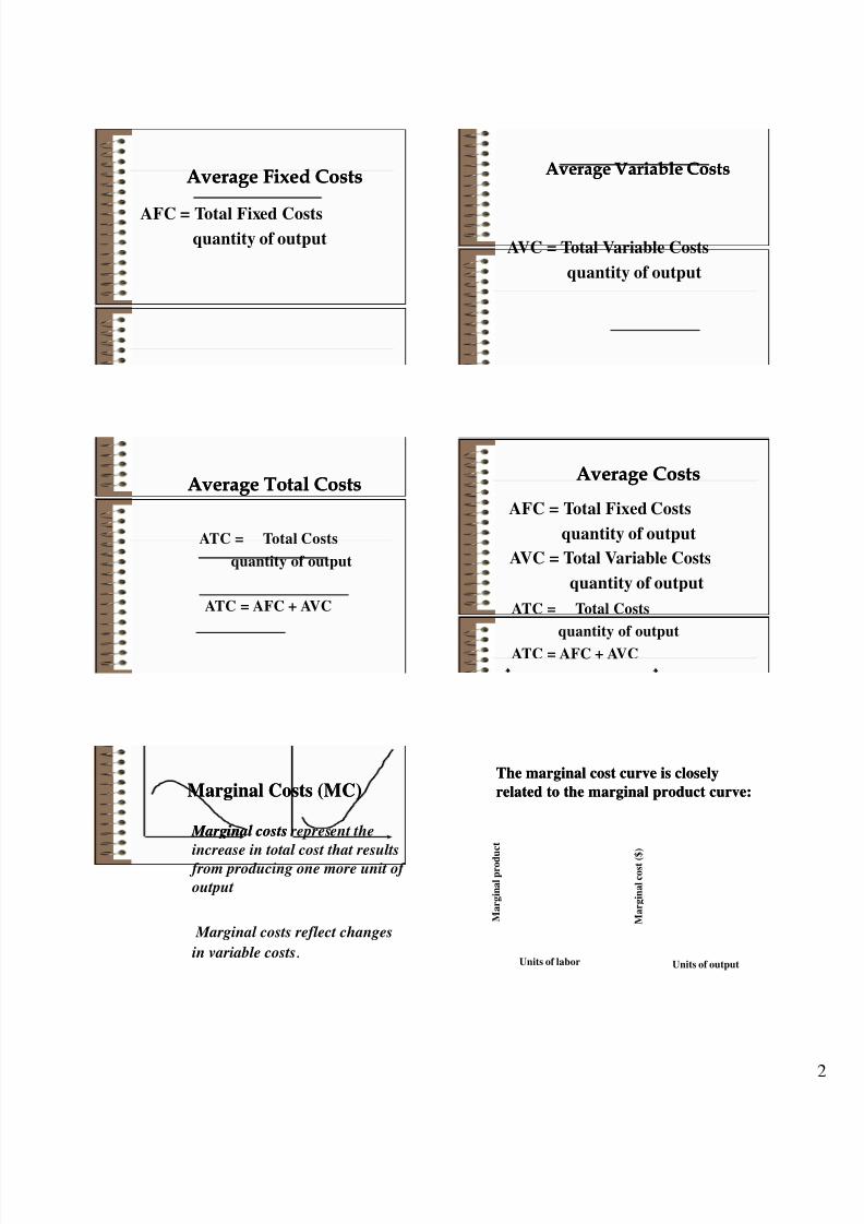
When marginal product begins to When marginal product begins tofall, marginal cost begins to rise:fall, marginal cost begins to rise:

Units of labor

M a r g i n a l p r o d u c t

M a r g i n a l c o s t ( $ )

Units of output

Diminishingreturnsset in. Diminishing

returnsset in.

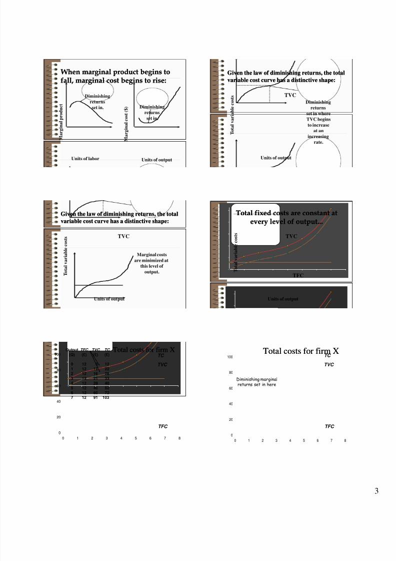
Given the law of diminishing returns, the totalGiven the law of diminishing returns, the total

variable cost curve has a distinctive shape:variable cost curve has a distinctive shape:

TVC

Units of output

T o t a l v a r i a b l e c o s t s

Diminishingreturns

set in whereTVC beginsto increase

at anincreasing

rate.

Given the law of diminishing returns, the totalGiven the law of diminishing returns, the totalvariable cost curve has a distinctive shape:variable cost curve has a distinctive shape:

TVC

Units of output


Marginal costsare minimized at

this level of output.

Total fixed costs are constant atTotal fixed costs are constant atevery level of output...every level of output...


Units of output

TVC

TFC

0

20

40

60

80

100

0 1 2 3 4 5 6 7 8

TC

Output(Q)

012345

67

TFC

(£)

121212121212

1212

TVC

(£)

01016212840

6091

TC

(£)

122228334052

72103

TVC

TFC

Total costs for firm XTotal costs for firm X

0

20

40

60

80

100

0 1 2 3 4 5 6 7 8

TC

TVC

TFC

Diminishing marginalreturns set in here




But average fixed costs decline asBut average fixed costs decline asoutput increases.output increases.

A v e r a g e f i x e d c o s t s

Units of output

AFC = Total Fixed Costsquantity of output

AFC

Average and marginal physical product

O u t p u t

Quantity of the variable factor

MPP

b

c

APP

Output (Q )

C o s t s ( £ )

MC

x

Marginal costMarginal costMarginal costMarginal cost

Diminishing marginalreturns set in here

0

20

40

60

80

100

0 1 2 3 4 5 6 7 8

TC

TVC

TFC

Bottom ofthe MC curve


Short-Run Costs

Marginal cost

– marginal cost ( MC ) and the law of diminishing returns

– the relationship between the marginal and total costcurves

Average cost

– average fixed cost ( AFC )

– average variable cost ( AVC )

– average (total) cost ( AC )

– relationship between AC and MC

Average total and average variableAverage total and average variable

costs are also affected by the law of costs are also affected by the law of

diminishing returns.diminishing returns.

Units of output

$$ MC ATC

AVC



Output (Q )

C o s t s ( £ )

AFC

AVC

MC

x

AC

z

y

Average and marginal costs Some important points aboutSome important points about

cost curves:cost curves:

Average total cost equals marginal cost

where average total cost is minimized.

Average variable cost equals marginal cost

where average variable cost is minimized.

The slope of the total variable cost curve

describes the change in TVC when output

increases by one unit.

The slope of the total variable cost curve is

equal to marginal cost.

Consider this shortConsider this short--run cost data forrun cost data fora hypothetical firm:a hypothetical firm:

q TVC MC AVC TFC TC AFC ATC

0 $ 0 $1000

1 10 1000

2 18 1000

3 24 1000

4 32 1000

5 42 1000

Can you fill in the missing columns?Can you fill in the missing columns?

Consider this shortConsider this short--run cost data forrun cost data fora hypothetical firm:a hypothetical firm:

Were you correct?Were you correct?

q TVC MC AVC TFC TC AFC ATC

0 $ 0 $-- $-- $1000 $1000 $-- $--

1 10 10 10 1000 1010 1000 1010

2 18 8 9 1000 1018 500 509

3 24 6 8 1000 1024 333 341

4 32 8 8 1000 1032 250 258

5 42 10 8.4 1000 1042 200 208

Long-run Average Cost

Inputs are variable, therefore all costsare variable.

Assumptions:1. Factor prices are given

2. The state of technology and factor qualityare given

3. Firms choose the least-cost combinationof factors for each output

LRAC

LRAC is U-shaped / basin-shaped. Each

SRAC sits on it or is tangent to it.

The LRAC consists a series of alternativeSRAC.

The firm can build in the LR any one of thedifferent sized plants. It can also alter the

size of plant



Relationship: LRAC & SRAC

LR a firm can build more factories, thus

experiencing economies of scale, the expansionenables / allows firm to produce with a new lowerSRAC curve.

Each SRAC corresponds to a particular amount of the factor that is fixed in the short-run.

Given time, the several expansions at varioustime period, enable a series of SRACs – From

these curves an envelope curve is developed.

LRAC

LRAC can take various shapes:

1. Economies of scale – LRAC will fall as the

scale of production increases

2. Diseconomies of scale – LRAC will rise as

output increases

3. Constant returns to scale /constant cost –

LRAC will be horizontal

OutputO

C o s t s

LRAC Economiesof scale

Constantcosts

Diseconomiesof scale

A typical long-run average cost curveTechnical Optimum

It is the point where AC for the plant sizeequals the MC of producing an extra unit. Itis the least cost point.

Where a firm’s MC < AC, increase inoutput will lower AC.

Where a firm’s MC > AC, increase inoutput will make AC higher I.e. each extraunit of production is costing more

Economies of large scale

productionA firm can enjoy economies of large scale

production when an increase in the size of the

operations reduces the cost per unit i.e. increasing

returns to scale flowing from internal economiesof scale.

The firm uses input more efficiently and is

considered as a cost advantage

Factors that bring about internal economies of

scale are as follows: (next slide please)

Economies of large scale production i.e.

Internal Economies of scale

More specialization of labour and

management

Better capital equipmentImproved management

Better use of raw materials

Greater use of by product and recycling

The introduction of new technology



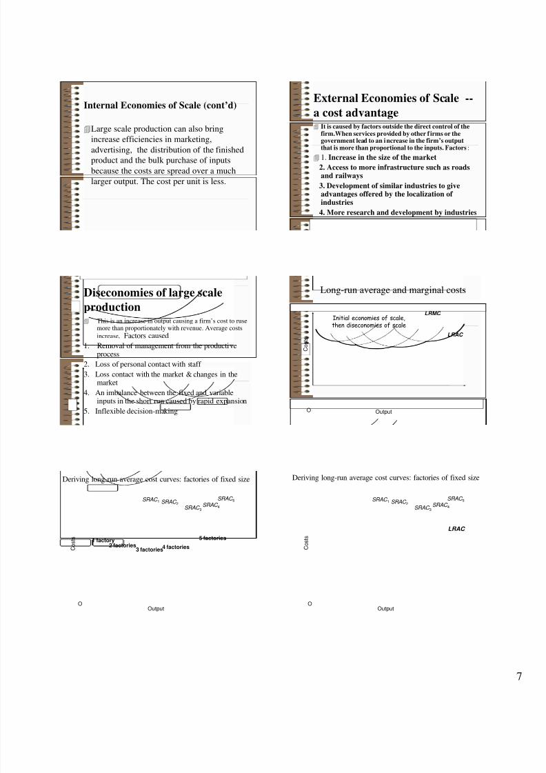
Internal Economies of Scale (cont’d)

Large scale production can also bring

increase efficiencies in marketing,

advertising, the distribution of the finishedproduct and the bulk purchase of inputs

because the costs are spread over a much

larger output. The cost per unit is less.

External Economies of Scale --

a cost advantage It is caused by factors outside the direct control of the

firm.When services provided by other f irms or thegovernment lead to an increase in the firm’s outputthat is more than proportional to the inputs. Factors:

1. Increase in the size of the market

2. Access to more infrastructure such as roadsand railways

3. Development of similar industries to giveadvantages offered by the localization of industries

4. More research and development by industries

Diseconomies of large scale

production This is an increase in output causing a firm’s cost to ruse

more than proportionately with revenue. Average costs

increase. Factors caused

1. Removal of management from the productiveprocess

2. Loss of personal contact with staff

3. Loss contact with the market & changes in themarket

4. An imbalance between the fixed and variableinputs in the short run caused by rapid expansion

5. Inflexible decision-making OutputO

C o s t s

LRMC

LRAC

Initial economies of scale,then diseconomies of scale

Long-run average and marginal costs

SRAC 3

C o s t s

OutputO

SRAC 4

SRAC 5

5 factories

4 factories3 factories2 factories1 factory

SRAC 1 SRAC 2

Deriving long-run average cost curves: factories of fixed size

SRAC 1

SRAC 3

SRAC 2 SRAC 4

SRAC 5

LRAC

C o s

t s

OutputO

Deriving long-run average cost curves: factories of fixed size



Revenue

Defining total, average and marginal

revenue

Revenue curves when firms are price takers(horizontal demand curve)

– average revenue ( AR)

– marginal revenue ( MR)

Output Decisions, Revenues, Costs,Output Decisions, Revenues, Costs,

and Profit Maximizationand Profit Maximization

Remember: Remember:

Firms operate in perfectly

competitive output markets.

In perfectly competitive

industries, prices are determined

in the market and firms are price

takers.

The demand curve for the firm is

perfectly elastic.

Total and Marginal RevenueTotal and Marginal Revenue

Total revenue is the amount of

revenue the firm takes in from the

sale of its product.

TR = price x quantity soldTR = price x quantity sold

Marginal revenue is the

additional revenue that a firm takes

in when it increases output by one

additional unit.

MR =MR = TR / TR / qq

In a perfectly competitive market, theIn a perfectly competitive market, the

firm’s demand curve is the firm’s marginalfirm’s demand curve is the firm’s marginalrevenue curve:revenue curve:

$5

S

D

Market

Units of output

$5

D=MR

Firm

Units of output

P r i c e p e r u n i t

Comparing Costs and Revenues toComparing Costs and Revenues to

Maximize ProfitMaximize Profit ::

$5

S

D

Market

Units of output

$5

D=MR

Firm

Units of output


The firm maximizes profits byThe firm maximizes profits byproducing whereproducing where MR = MCMR = MC ::

$5

S

D

Market

Units of output

$5

D=MR

Firm


Units of outputq*



Why is q=300 the profitWhy is q=300 the profit--maximizing levelmaximizing level

of output for the firm?of output for the firm?

$5

Firm

D=MR

Units of output

MC

300

ATC

250100 3400

$$

What will be the firm’s profit level at the What will be the firm’s profit level at theprofitprofit--maximizing level of output?maximizing level of output?

$5

Firm

D=MR

Units of output

MC

300

ATC

250100 3400

$$

$3.50

The firm’s profit at q=300 isThe firm’s profit at q=300 is$1.50 per unit, or $450.$1.50 per unit, or $450.

$5

Firm

D=MR

Units of output

MC

300

ATC

250100 3400

$$

$3.50

Consider the following data forConsider the following data fora hypothetical firm:a hypothetical firm:

q TFC TVC MC P=MR TR TC TR-TC

0 $10 $ 0 $-- $15

1 10 10 15

2 10 15 15

3 10 20 15

4 10 30 15

5 10 50 15

6 10 80 15Can you fill in the missing columns?

What is the firm’s profitWhat is the firm’s profit

maximizing level of output?maximizing level of output?

q TFC TVC MC P=MR TR TC TR-TC

0 $10 $ 0 $-- $15 $-- $10 $ -10

1 10 10 10 15 15 20 - 5

2 10 15 5 15 30 25 5

3 10 20 5 15 45 30 15

4 10 30 10 15 60 40 204 10 30 10 15 60 40 20

5 10 50 20 15 75 60 15

6 10 80 30 15 90 90 0

The Competitive Firm’s ShortThe Competitive Firm’s Short

Run Supply CurveRun Supply Curve

Units of output

MC

0

$$

ATC

P=MR and the firm

produces where

MC=P=MR. Thus the

firm’s supply curve is

its marginal cost curve

- above AVC.

= S



If price falls below AVC, theIf price falls below AVC, thefirm should produce no output.firm should produce no output.

Units of output

MC

0

$$

ATC

This will be exploredmore carefully in the

Why?0

4

8

12

16

20

0 1 2 3 4 5 6 7

TR

Elasticity = -1

Quantity

T R ( £ )

TR curve for a firm facing a downward-sloping D curve

-4

-2

0

2

4

6

8

1 2 3 4 5 6 7

Elasticity = -1

Elastic

Inelastic

A R , M R ( £ )

Quantity

MR

AR

AR and MR curves for a firm facing a downward-sloping D curve

Profit

Profit

Maximization

-8

-4

0

4

8

12

16

20

24

1 2 3 4 5 6 7

T R , T

C , T Π ( £ )

T Π

TR

TC

d

e

f

Quantity

Finding maximum profit using total curves

-4

0

4

8

12

16

1 2 3 4 5 6 7

Quantity

C o s t s a n d r e

v e n u e ( £ )

e

MR

MC

Profit-maximisingoutput

Finding the profit-maximising output using marginal curves



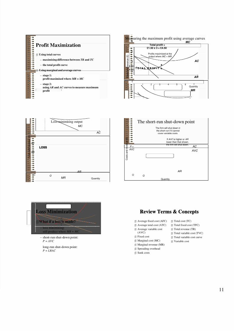
Profit Maximization

Using total curves

– maximising difference between TR and TC

– the total profit curve

Using marginal and average curves

– stage 1:profit maximised where MR = MC

– stage 2:using AR and AC curves to measure maximumprofit

6.00

4.50

-4

0

4

8

12

16

1 2 3 4 5 6 7

T O T A L P R O F I TT O T A L P R O F I T

MR

Quantity

C o s t s a n d r e v e n u e ( £ )

MC

AC

AR

b

a

Total profit =£1.50 x 3 = £4.50

Measuring the maximum profit using average curves

Profits maximised at theoutput where MC = MR

O


Quantity

MC

AC

AR

MR Q

AC

AR

LOSSLOSS

Loss-minimising output

O


Quantity

AR

AVC

AC P =

AVC

Q

The short-run shut-down pointThe firm will shut down inthe short run if it cannot

cover variable costs.

If AVC is higher or AR

lower than that shown,the firm will shut down.

Loss Minimization

What if a loss is made?

– loss minimising:

still produce where MR = MC

– short-run shut-down point:P = AVC

– long-run shut-down point:P = LRAC

Review Terms & ConceptsReview Terms & Concepts

Average fixed cost (AFC)

Average total cost (ATC)

Average variable cost

(AVC) Fixed cost

Marginal cost (MC)

Marginal revenue (MR)

Spreading overhead

Sunk costs

Total cost (TC)

Total fixed cost (TFC)

Total revenue (TR)

Total variable cost (TVC)

Total variable cost curve

Variable cost

200901 Eco The Money Supply and the Federal Reserve System

Documents

Transcript of 200901 Eco The Money Supply and the Federal Reserve System