134489_FR

Ice P

Glas

Preven

ss City

Douglas K

ntion o

y Skyw

K. Nims, V

or Rem

way Ca

Victor J. H

1

moval o

ables

Hunt, Arth

The OhioOffice of

on the

hur J. Helm

o DepartmStatewide

Stat

Veter

micki, Tsu

ment of Tre Planning

te Job Nu

ran's

Preparedun-Ming T

Preparedransportatg & Resea

mber 134

August 2

Final Re

d by: . Ng

d for: tion, arch

4489

2014

eport

2

Technical Report Documentation Page

1. Report No. 2. Government Accession No. 3. Recipient's Catalog No.

FHWA/OH-2014/11

4. Title and Subtitle 5. Report Date (Month and Year)

Ice Prevention or Removal on the Veterans Glass City Skyway Cables

August 2014

6. Performing Organization Code

7. Author(s) 8. Performing Organization Report No.

Douglas Nims, Victor Hunt, Arthur Helmicki, Tsun-Ming Ng

9. Performing Organization Name and Address 10. Work Unit No. (TRAIS)

University of Toledo2801 W. Bancroft St.Toledo, OH 43606

11. Contract or Grant No.

SJN 134489

12. Sponsoring Agency Name and Address 13. Type of Report and Period Covered

Ohio Department of TransportationResearch Section1980 West Broad St., MS 3280Columbus, OH 43223

Final Report

14. Sponsoring Agency Code

15. Supplementary Notes

16. Abstract

The Veteran’s Glass City Skyway is a cable - stayed bridge in Toledo, Ohio owned by the Ohio DOT. Five times in the seven winters the VGCS has been in service, ice has formed on the stay cables. Ice up to 3/4” thick and conforming to the cylindrical shape of the stay has formed. As the stays warm, ice sheds in curved sheets that fall and can be blown across the bridge. The falling ice sheets pose a potential hazard and may require lane or bridge closure. Because of the specialized knowledge required, this problem required a team including experts in icing, the VGCS construction, the structural measurement system on the bridge, and green technology. The VGCS stay sheaths are made of stainless steel, have a brushed finish, lack the usual helical spiral and have a large diameter. No existing ice anti/deicing technology was found to be practical. Therefore, ODOT elected to manage icing administratively. A real-time ice monitoring system for local weather conditions on the VGCS and the stays was designed. The system collects data from sensors on the bridge and in the region. The study of the past weather and icing events lead to quantitative guidelines about when icing accretion and shedding were likely. The monitoring system tracked the icing conditions on the bridge with a straightforward interface so information on the icing of the bridge is available to the bridge operators. If the conditions favorable to icing occurred, the monitoring system notified the research team and appropriate ODOT officials. If ice has formed, the monitor tracks the conditions that might lead to ice fall.

17. Key Words 18. Distribution Statement

Ice, Bridges, Cable-stayed, Hazard Mitigation, Ice Removal, Ice Prevention

No restrictions. This document is available to the public through the National Technical Information Service, Springfield, Virginia 22161

Form DOT F 1700.7 (8-72) Reproduction of completed pages authorized

19. Security Classif. (of this report) 20. Security Classif. (of this page) 21. No. of Pages 22. Price

Unclassified Unclassified 316 $ 652,894.58

3

Ice Prevention or Removal on the Veteran's

Glass City Skyway Cables

Prepared by: Douglas K. Nims

University of Toledo

Victor J. Hunt University of Cincinnati

Arthur J. Helmicki University of Cincinnati

Tsun-Ming T. Ng, Ph.D., P.E. University of Toledo

August 2014

Prepared in cooperation with the Ohio Department of Transportation and the U.S. Department of Transportation, Federal Highway Administration

The contents of this report reflect the views of the author(s) who is (are) responsible for the facts and the

accuracy of the data presented herein. The contents do not necessarily reflect the official views or

policies of the Ohio Department of Transportation or the Federal Highway Administration. This report

does not constitute a standard, specification, or regulation.

4

Acknowledgments

The authors would like to acknowledge the University of Toledo graduate students Mr. Ali Arbabzadegan, Mr. Joshua Belknap, Mr. Nutthavit Likitkumchorn, and Mr. Clinton and University of Cincinnati Infrastructure Institute graduate students, Mr. Shekhar Agrawal, Mr. Biswarup Deb, Mr. Jason Kumpf and Ms. Chandrasekar Venkatesh, who played a significant role in the research and the writing of this report. Chapter 1, Introduction, was primarily written by Mr. Ali Arbabzadegan with contributions from Mr. Clinton Mirto. Chapter 3, Phase I Research, was primarily written by Mr. Arbabzadegan with contributions from Mr. Joshua Belknap and Mr. Clinton Mirto. Chapter 4, Weather Background, Modeling, and Analysis, was written by Mr. Belknap with contributions from Mr. Arbabzadegan, and Mr. Mirto. Chapter 5, Development of the VGCS Dashboard and Initial Dashboard Results was written by students from UCII. Chapter 6, New Local Weather Sensor Testing, was written by students from UCII. Chapter 7, Experimental Studies on the Sheath Specimens, primarily written by Mr. Arbabzadegan, Mr. Likitkumchorn and students from UCII. Chapter 8, Deployment of New Sensors and Upgrade of Dashboard, was written by Mr. Arbabzadegan and students from UCII. Chapter 9, Sensor Development, was written by Mr. Likitkumchorn. Mr. Mirto assisted in the editing of this report.

University of Cincinnati graduate students Mr. Biswarup Deb, Mr. Chandrasekar Venkatesh, Mr. Nithyakumaran Gnanasekar, and Ms. Monisha Baskaran were instrumental in maintaining and updating the Dashboard for this past winter and delivering the standalone computer system to ODOT

Dr. Sridhar Viamajala graciously allowed the Scott Park Icing Experiment Station to be built on an unoccupied portion of the concrete pad used for his sustainable energy research.

This project was performed under the aegis of the University of Toledo – University Transportation Center. The continuous support of Director Richard Martinko and Associate Director Christine Lonsway has made this project possible.

The authors thank Ms. Kathleen Jones and Dr. Charles Ryerson of the U.S. Army Cold Regions Research and Engineering Laboratory for the frequent discussions about the project and extensive analysis, support in developing the criteria for the ice fall dashboard, and their help in the editing of this report.

This project was sponsored and supported by the Ohio Department of Transportation. The authors gratefully acknowledge their financial support. Mr. Mike Gramza, P.E. and Mr. Tim Keller, P.E. were the technical liaisons and the authors appreciate their support and input throughput the project. The author would also like to thank Mr. Mike Madry, Mr. Dave Kanavel and Mr. Matt Harvey from ODOT for access to the bridge and assistance in observing the icing events and Mr. Jeff Baker, P.E. (now retired from ODOT) for his assistance in defining criteria for the ice fall dashboard and reviewing the User Manual

5

Dedication

This report is dedicated to the late Professor K. Cyril ‘Cy’ Masiulaniec of Mechanical, Industrial, and Manufacturing Engineering of the University of Toledo. Cy was one of the initial investigators on this project and he was active until the week before his passing when he developed the final details and directions for mounting the thermistors. He will be remembered for his attention to detail and patient thorough explanations of the thermal science that made a significant contribution to this project.

Cy was always willing to step up and help our students, his department and the college in many ways. UT students consistently recognized him as an outstanding teacher and he received the UT College of Engineering Award for Teaching Excellence.

6

Abstract

The Veteran’s Glass City Skyway (VGCS) is a large cable - stayed bridge in Toledo, Ohio owned by the Ohio Department of Transportation (ODOT). The VGCS carries I-280 over the Maumee River. Five times in the seven winters the VGCS has been in service, ice has formed on the stay cable sheaths. Ice accumulations have been up to approximately 3/4” thick and the ice conforms to the cylindrical shape of the stay sheath. As the stays warm, they shed the ice in curved sheets that fall up to two hundred and fifty feet to the roadway and the pieces of ice can be blown across several lanes of traffic on the bridge deck. The falling ice sheets require lane closures or even closure of the entire bridge and could present a potential hazard to the traveling public.

Because of the unique nature of the problem, the need for a quick response and the specialized nature of the icing knowledge required, this problem has been addressed with an expert team. The team includes experts in icing from the U.S. Army Cold Regions Research and Engineering Laboratory and the NASA Glenn Icing Branch, the ODOT project managers from the bridge construction, the engineers who designed and implemented the existing structural strain measurement system on the bridge, and experts in green technology.

The stay sheaths of the VGCS are unique: they are made of stainless steel, have a brushed finish, lack the usual helical spiral and have a large diameter. No existing ice anti/deicing technology was found to be practical for the VGCS. Therefore, ODOT elected to manage icing administratively.

To do this, the research team designed a real-time monitoring system for local weather conditions on the VGCS and the stays as well as the surrounding area. The monitoring system collects a comprehensive set of data from local sensors on the bridge as well as other sensors in the Toledo region. The study of the past weather and icing events lead to quantitative guidelines about the weather conditions that made icing accretion and shedding likely. These guidelines form the core of the algorithms in the ice monitoring system implemented on the bridge. The monitoring system tracked the icing conditions on the bridge with a straightforward interface so information on the icing of the bridge is readily available to the bridge operators. If the conditions favorable to icing occurred, the monitoring system notified the research team and appropriate ODOT officials. If ice forms, the monitor tracks the conditions that might lead to ice fall.

The benefits of completing this project include observations of an icing event, review of historical icing events, a building a local weather station on the bridge and stays to collect real-time data on icing and developing the monitoring system. Because no commercial sensor for directly measuring the presence or state of ice on the sheath exists, an electrical resistance based sensor has been developed.

7

Table of Contents

Cover Sheet .................................................................................................................. 12

Technical Report Documentation Page ........................................................................... 2

Disclaimer ....................................................................................................................... 3

Acknowledgments ........................................................................................................... 4

Dedication ....................................................................................................................... 5

Abstract ........................................................................................................................... 6

Table of Contents ............................................................................................................ 7

List of Figures ................................................................................................................ 12

List of Tables ................................................................................................................. 19

Chapter 1: Introduction ................................................................................................. 21

Section 1.1: Bridge Background ............................................................................... 21

Section 1.2: Summary of Goals and Objectives ....................................................... 24

Section 1.3: Summary of Results.............................................................................. 25

Section 1.4: Organization of this Report ................................................................... 27

Chapter 2: Goals, Objectives, Research Approach and Benefits ................................. 29

Section 2.1: Overview of Chapter ............................................................................. 29

Section 2.2: Goal ...................................................................................................... 29

Section 2.3: Objectives ............................................................................................. 29

Section 2.4: Expert Team Approach to the Research ............................................... 33

Section 2.5: Benefits ................................................................................................. 36

Section 2.6: Chapter Summary ................................................................................. 37

Chapter 3: Phase I Research ....................................................................................... 39

Section 3.1: VGCS Sheaths ..................................................................................... 39

Section 3.2: Literature Review .................................................................................. 40

Section 3.2.1 Known Icing Problems on Other Bridges .......................................... 40

Section 3.2.2 Anti-Icing/Deicing Technologies found in literature .......................... 41

Section 3.3: Technology Matrix ................................................................................ 48

Section 3.4: Sensors on the VGCS........................................................................... 50

Section 3.4.1: Sensors on the VGCS prior to the 2012 – 2013 Winter .................. 50

Section 3.4.2: Sensors added in 2012 – 2013 ....................................................... 51

Section 3.4.3: Sensors added in 2013 – 2014 ....................................................... 51

Section 3.5: Chapter Summary ................................................................................. 53

Chapter 4: Weather History, Modeling and Analysis .................................................... 55

8

Section 4.1: Introduction ........................................................................................... 55

Section 4.2: Description of the basic weather that gives rise to an ice storm ........... 55

Section 4.3: VGCS Weather History ......................................................................... 56

Section 4.4: Lessons Learned from Previous Icing Events ........................................ 73

Section 4.5: Analysis ................................................................................................ 74

Section 4.6: Chapter Summary .................................................................................. 76

Chapter 5: Development of the VGCS Dashboard and Initial Dashboard Results ....... 77

Section 5.1: Introduction ............................................................................................ 77

Section 5.2: Weather Data ................................................................................... 80

Section 5.2.1: Introduction ................................................................................... 80

Section 5.2.2: Data Sources ................................................................................ 80

Section 5.2.3: Data Classification ........................................................................... 83

Section 5.2.4: Data Collection and Storage .......................................................... 86

Section 5.3: Ice Accumulation Determination Algorithm ........................................... 87

Section 5.3.1: Data Update Time ........................................................................... 88

Section 5.3.2: Ice Accumulation Algorithm ............................................................. 88

Section 5.3.3: Station Individual Weights .............................................................. 89

Section 5.3.4: Threshold weights ........................................................................... 90

Section 5.3.5: Ice Shedding ................................................................................... 91

Section 5.4: Ice Persistence Algorithm ...................................................................... 91

Section 5.4.1: Ice States ........................................................................................ 91

Section 5.4.2: Ice Accumulation Persistence Algorithm ......................................... 92

Section 5.4.3: Ice Presence Confirmation .............................................................. 95

Section 5.4.4: Ice Shedding Persistence Algorithm................................................ 96

Section 5.5: Monitor Website .................................................................................... 99

Section 5.5.1: Dashboard Main Panel .................................................................. 100

Section 5.5.2: Weather Map ................................................................................. 101

Section 5.5.3: History ........................................................................................... 103

Section 5.5.4: Implementation Tools .................................................................... 104

Section 5.6: Performance Testing ........................................................................... 104

Section 5.6.1: System Reliability Test .................................................................. 104

Section 5.6.2: Ground Truth ................................................................................. 106

Section 5.7: Conclusions ........................................................................................ 125

Chapter 6: New Local Weather Sensor Testing .......................................................... 126

9

Section 6.1: Introduction .......................................................................................... 126

Section 6.1.1: Geokon Thermistors ...................................................................... 126

Section 6.1.2: Dielectric Wetness Sensor ............................................................ 127

Section 6.1.3: Solar Radiation or Sunshine Sensor ............................................. 127

Section 6.1.4: Rain Tipping Bucket ...................................................................... 128

Section 6.1.5: Goodrich Ice Detector ................................................................... 128

Section 6.2: Geokon Thermistor 3800-2-2 ............................................................... 129

Section 6.2.1: Laboratory experiment on temperature measurement using Geokon Thermistors .......................................................................................................... 130

Section 6.2.2: Installation of Geokon Thermistors 3800-2-2 at the VGCS on Stays 8 & 20 ...................................................................................................................... 135

Section 6.3: LWS-L Dielectric Leaf Wetness Sensor .............................................. 145

Section 6.3.1: Laboratory experiment on measurement of output voltage using LWS-L Leaf Wetness Sensor. .............................................................................. 145

Section 6.4: Sunshine Sensor BF5 .......................................................................... 149

Section 6.4.1: Laboratory experiment on measurement of solar radiation using Sunshine Sensor BF5. ......................................................................................... 150

Section 6.5: Met One Rain Tipping Bucket .............................................................. 153

Section 6.5.1: Laboratory experiment on measurement of precipitation using Tipping Bucket ..................................................................................................... 154

Section 6.6: Goodrich Ice Detector .......................................................................... 156

Section 6.6.1: Laboratory experiment on measurement of ice presence/thickness using Goodrich Ice Detector 0872F1 .................................................................... 157

Section 6.7: Conclusions ........................................................................................ 161

Chapter 7: Field Study of Temperature Effect on Stay Sheaths .................................. 162


Section 7.2: Design of Icing Experiment Station ...................................................... 162

Section 7.3: Design of the UT Icing Tunnel and Design .......................................... 164

Section 7.4: Icing Accretion and shedding Experiments at Scott Park..................... 168

Section 7.5: Thermal Experiments at Scott Park ..................................................... 172

Section 7.6: Anti/de-icing Fluid Experiments at Scott Park ...................................... 175

Section 7.7: Coating Experiments at Scott Park ...................................................... 176

Section 7.8: Coating Experiments using Icing UT Tunnel ........................................ 178

Section 7.8.1: Testing Procedure ............................................................................ 178

Section 7.8.2: Experiments – Icing Progression ...................................................... 179

Section 7.8.3: Result Summery of Icing Tunnel Coating Tests ................................ 199

10

Section 7.9: Field Experiment Trips ......................................................................... 200

Section 7.10: Conclusions ....................................................................................... 211

Chapter 8: Deployment of New Sensors and Upgrade of the Dashboard .................. 213


Section 8.2: Self Supporting Instrumentation Tower Design .................................... 213

Section 8.2.1: Tower Design ................................................................................ 213

Section 8.2.2: Anchorage System Design ............................................................ 214

Section 8.3: VGCS Ice Sensors Bridge Installation trip (May 16-17, 2013) ............. 215

Section 8.4: Changes to the Ice Accumulation Algorithm ........................................ 220

Section 8.5: Changes to the Ice Shedding Algorithm............................................... 225

Section 8.6: Changes to the Dashboard .................................................................. 227

Section 8.6.1: Dashboard Main Panel .................................................................. 228

Section 8.6.2: Map (Weather Data by location) .................................................... 229

Section 8.6.3: New Sensors Plotting .................................................................... 231

Section 8.7: Insights Gained from the Operation of the Upgraded Dashboard ........ 235

Section 8.7.1: Ice Events (Winter 2013/2014) ...................................................... 236

Section 8.7.2: Sensor Performance ..................................................................... 244

Section 8.7.3: Issues and Observations from Winter Performance ...................... 249

Section 8.8: Conclusions ......................................................................................... 250

Chapter 9: Ice Presence and State Sensor Development ........................................... 252


Section 9.2: Ice Presence and State Sensor Laboratory Testing ............................ 252

Section 9.2.1: Sensors and Data Acquisition System .............................................. 252

Section 9.2.2: Design of Experiments ...................................................................... 254

Section 9.2.3: Laboratory Test Results .................................................................... 257

Section 9.3: UT Icing Sensor in Full Scale Experiments .......................................... 265

Section 9.3.1: Specimens and Data Acquisition System Setup ............................... 266

Section 9.3.2: Full Scale Outdoor Tests .................................................................. 270

Section 9.3.3 Full Scale Experiments Result ........................................................... 272

Section 9.4: Conclusion and Next Steps .................................................................. 275

Chapter 10: Transition and Maintenance .................................................................... 276

Section 10.1: Introduction ....................................................................................... 276

Section 10.2: Standalone Computer System ......................................................... 276

Section 10.3: Maintenance ...................................................................................... 276

11

Chapter 11: Conclusion, Benefits, Implementation and Future Work .......................... 279

Section 11.1: Summary of Goals and Objectives .................................................... 279

Section 11.2: Results ............................................................................................... 280

Section 11.3 Benefits ............................................................................................... 284

Section 11.4: Implementation .................................................................................. 285

Section 11.5: Transition and Long Term Maintenance ............................................ 286

Section 11.6: Archiving of Supporting Documents ................................................... 286

Section 11.7: Recommendations for Future Work ................................................... 286

Bibliography ................................................................................................................ 289

Appendix A: Technology Matrix ................................................................................... 306

12

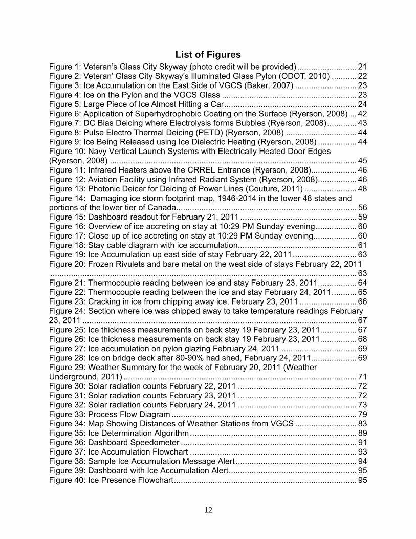
List of Figures Figure 1: Veteran’s Glass City Skyway (photo credit will be provided) .......................... 21 Figure 2: Veteran’ Glass City Skyway’s Illuminated Glass Pylon (ODOT, 2010) ........... 22 Figure 3: Ice Accumulation on the East Side of VGCS (Baker, 2007) ........................... 23 Figure 4: Ice on the Pylon and the VGCS Glass ........................................................... 23 Figure 5: Large Piece of Ice Almost Hitting a Car .......................................................... 24 Figure 6: Application of Superhydrophobic Coating on the Surface (Ryerson, 2008) ... 42 Figure 7: DC Bias Deicing where Electrolysis forms Bubbles (Ryerson, 2008) ............. 43 Figure 8: Pulse Electro Thermal Deicing (PETD) (Ryerson, 2008) ............................... 44 Figure 9: Ice Being Released using Ice Dielectric Heating (Ryerson, 2008) ................. 44 Figure 10: Navy Vertical Launch Systems with Electrically Heated Door Edges (Ryerson, 2008) ............................................................................................................ 45 Figure 11: Infrared Heaters above the CRREL Entrance (Ryerson, 2008) .................... 46 Figure 12: Aviation Facility using Infrared Radiant System (Ryerson, 2008) ................. 46 Figure 13: Photonic Deicer for Deicing of Power Lines (Couture, 2011) ....................... 48 Figure 14: Damaging ice storm footprint map, 1946-2014 in the lower 48 states and portions of the lower tier of Canada............................................................................... 56 Figure 15: Dashboard readout for February 21, 2011 ................................................... 59 Figure 16: Overview of ice accreting on stay at 10:29 PM Sunday evening .................. 60 Figure 17: Close up of ice accreting on stay at 10:29 PM Sunday evening ................... 60 Figure 18: Stay cable diagram with ice accumulation.................................................... 61 Figure 19: Ice Accumulation up east side of stay February 22, 2011 ............................ 63 Figure 20: Frozen Rivulets and bare metal on the west side of stays February 22, 2011 ...................................................................................................................................... 63 Figure 21: Thermocouple reading between ice and stay February 23, 2011 ................. 64 Figure 22: Thermocouple reading between the ice and stay February 24, 2011 ........... 65 Figure 23: Cracking in ice from chipping away ice, February 23, 2011 ......................... 66 Figure 24: Section where ice was chipped away to take temperature readings February 23, 2011 ........................................................................................................................ 67 Figure 25: Ice thickness measurements on back stay 19 February 23, 2011 ................ 67 Figure 26: Ice thickness measurements on back stay 19 February 23, 2011 ................ 68 Figure 27: Ice accumulation on pylon glazing February 24, 2011 ................................. 69 Figure 28: Ice on bridge deck after 80-90% had shed, February 24, 2011 .................... 69 Figure 29: Weather Summary for the week of February 20, 2011 (Weather Underground, 2011) ...................................................................................................... 71 Figure 30: Solar radiation counts February 22, 2011 .................................................... 72 Figure 31: Solar radiation counts February 23, 2011 .................................................... 72 Figure 32: Solar radiation counts February 24, 2011 .................................................... 73 Figure 33: Process Flow Diagram ................................................................................. 79 Figure 34: Map Showing Distances of Weather Stations from VGCS ........................... 83 Figure 35: Ice Determination Algorithm ......................................................................... 89 Figure 36: Dashboard Speedometer ............................................................................. 91 Figure 37: Ice Accumulation Flowchart ......................................................................... 93 Figure 38: Sample Ice Accumulation Message Alert ..................................................... 94 Figure 39: Dashboard with Ice Accumulation Alert ........................................................ 95 Figure 40: Ice Presence Flowchart ................................................................................ 95

13

Figure 41: Ice Shedding Flowchart ................................................................................ 97 Figure 42: Sample Ice Shedding Message Alert ........................................................... 98 Figure 43: Dashboard with Ice Shedding Alert .............................................................. 99 Figure 44: State Transitions possible from Red Level 3 ................................................ 99 Figure 45: Dashboard Main Panel ............................................................................... 101 Figure 46: Dashboard History Panel ........................................................................... 103 Figure 47: Weather Summary on Feb 20, 2011 .......................................................... 107 Figure 48: Screenshot Showing Ice Accretion on VGCS ............................................. 108 Figure 49: Weather Summary on Feb 21, 2011 .......................................................... 109 Figure 50: Weather Summary on Feb 22, 2011 .......................................................... 110 Figure 51: Ice Accumulation on Stays on Feb 22, 2011 .............................................. 110 Figure 52: Weather Summary on Feb 24, 2011 .......................................................... 112 Figure 53: Example of Ice Shedding Alert ................................................................... 112 Figure 54: Ice Falling from VGCS on Feb 24, 2011 ................................................... 113 Figure 55: Weather Summary on Feb 25, 2011 .......................................................... 114 Figure 56: Feb 24, 2011 Algorithm Performance Graph .............................................. 115 Figure 57 : Contribution of the Icing Criteria and Weather Stations ............................ 116 Figure 58: Solar Radiation Variation on Feb 24, 2011 ................................................ 117 Figure 59: Features of the Past Icing Events .............................................................. 119 Figure 60: Dec 12, 2007 Algorithm Performance Graph ............................................. 120 Figure 61: Mar 28, 2008 Algorithm Performance Graph .............................................. 122 Figure 62: Dec 17, 2008 Algorithm Performance Graph ............................................. 123 Figure 63: Jan 03, 2009 Algorithm Performance Graph .............................................. 124 Figure 64: Geokon 3800-2-2 Thermistor ..................................................................... 130 Figure 65: Naked Thermistor Bead (photo credits, John Flynn, Geokon Inc.) ............. 130 Figure 66: Canary Systems Multilogger Software ....................................................... 131 Figure 67: Measurement trend of eight thermistors ..................................................... 132 Figure 68: Thermistors kept in freezer ......................................................................... 133 Figure 69: Thermistors immersed in water left to freeze ............................................. 133 Figure 70: Readings simultaneously noted by handheld GK 404 ................................ 133 Figure 71: Standard thermometer immersed in setup to record temperature .............. 133 Figure 72: Thermistor Characteristics at Freezing ...................................................... 134 Figure 73: Side View of Gage Locations at VGCS ...................................................... 135 Figure 74: Custon Thermistor Mount Fabricated for Installing on Stay Surface .......... 136 Figure 75: Thermistor Placed on East Side of Stay ..................................................... 136 Figure 76: Thermistors Placed on Upper Side of Stay ................................................ 136 Figure 77: Far View of Thermistor Installation of Stay ................................................. 137 Figure 78: Thermistor Cables Being Routed to Multiplexer Inside White Box ............. 137 Figure 79: Stay Sheath Cross Section Showing Thermistor Positions ........................ 138 Figure 80: Stay 20 Thermistors Temperature Trend ................................................... 139 Figure 81: Stay 8 Thermistors Temperature Trend ..................................................... 140 Figure 82: Characteristics for Stay 20 Thermistors on March 15 ................................ 143 Figure 83: Characteristics for Stay 20 thermistors on March 9 & 10 ........................... 144 Figure 84: Leaf Wetness Sensor functional diagram ................................................... 145 Figure 85: Experimental setup of data logger CR1000 with LWS-L Leaf Wetness Sensor .................................................................................................................................... 146

14

Figure 86: Droplets of Water Sprinkled on Leaf .......................................................... 146 Figure 87: LWS-L partially immersed in cup of water .................................................. 147 Figure 88: LWS-L immersed in cup left to freeze ........................................................ 147 Figure 89: LWS Wetness Test .................................................................................... 148 Figure 90: LWS Freezing Temperature Test ............................................................... 148 Figure 91: Sunshine Sensor BF5 (side view) and Detailed Construction .................... 149 Figure 92: Sunshine Sensor BF5 Set Up on a Deck for Unobstructed Exposure to Solar Radiation ..................................................................................................................... 150 Figure 93: Solar radiation characteristics over an extended period of 16 days ........... 151 Figure 94: A typical partly cloudy day chosen to see the daily solar radiation characteristics ............................................................................................................. 152 Figure 95: A typical clear sunny day taken as example to see the daily solar radiation characteristics ............................................................................................................. 153 Figure 96: Rain Tipping Bucket (from top left clockwise) distant view, top view and inside view ................................................................................................................... 154 Figure 97: Rain Bucket lab .......................................................................................... 155 Figure 98: Gessler Buret ............................................................................................. 155 Figure 99: Rain Bucket accuracy experiment (actual vs tipping volume) .................... 156 Figure 100: The Goodrich Ice Detector (external and function diagrams) ................... 157 Figure 101: Ice Detector Mounted for Experiment ....................................................... 159 Figure 102: Microcare Anti-Stat Freezing Spray ......................................................... 159 Figure 103: Probe before Spraying ............................................................................. 159 Figure 104: Probe After Spraying ................................................................................ 159 Figure 105: Frequency/Ice thickness characteristics of 0872F1 during freezing spray experiment .................................................................................................................. 160 Figure 106: Thickness measurement using calipers ................................................... 160 Figure 107: Google Earth Screenshot of Scott Park ................................................... 162 Figure 108: Experimental Setup .................................................................................. 163 Figure 109: Sensors on South-faced Specimen .......................................................... 164 Figure 110: Data Acquisition System .......................................................................... 164 Figure 111: SolidWorks Design for the UT Icing Tunnel .............................................. 165 Figure 112: UT Icing Tunnel ........................................................................................ 165 Figure 113: Testing Section of the UT Icing Tunnel .................................................... 166 Figure 114: Misting System in the Testing Section ..................................................... 167 Figure 115: Panasonic HX_A100D Camera (Panasonic 2013) ................................... 167 Figure 116: Mounting System of Testing Section ........................................................ 168 Figure 117: Spraying a Mist of Water on North-faced Specimen ................................ 168 Figure 118: Pattern of Ice Accumulation on Outdoor Tests ......................................... 169 Figure 119: Water beneath the Ice Layer before Shedding ......................................... 169 Figure 120: Ice Shedding Steps .................................................................................. 170 Figure 121: Stay’s Behavior in Icing Test – 2/15 to 2/18 ............................................. 171 Figure 122: Stay’s Behavior in Icing Test – 2/20 to 2/22 ............................................. 171 Figure 123: Thermal Experiment Setup ....................................................................... 173 Figure 124: Strands Configuration in Thermal Tests ................................................... 173 Figure 125: Deicing Pattern in Thermal Test ............................................................... 174 Figure 126: Accumulated Ice in Anti-icing Thermal Test ............................................. 174

15

Figure 127: Formation of Ice in Chemical Anti-icing Test ............................................ 175 Figure 128: Drip Tube System used in Chemical Deicing Test ................................... 176 Figure 129: Hydrobead Sprayed on Half of the Specimen .......................................... 177 Figure 130: Water Droplets due to Hydrobead ............................................................ 177 Figure 131: Specimen’s Behavior in Coating Test ...................................................... 178 Figure 132: Uncoated - 40 Micron - 0:00 min .............................................................. 179 Figure 133: Uncoated - 40 Micron - 0:15 min .............................................................. 179 Figure 134: Uncoated - 40 Micron - 0:30 min .............................................................. 180 Figure 135: Uncoated - 40 Micron - 0:45 min .............................................................. 180 Figure 136: Uncoated - 40 Micron – 1:00 min ............................................................. 180 Figure 137: Uncoated - 40 Micron – 1:30 min ............................................................. 181 Figure 138: Uncoated - 40 Micron – 2:00 min ............................................................. 181 Figure 139: Uncoated - 40 Micron – 4:00 min ............................................................. 181 Figure 140: Uncoated - 40 Micron – 6:00 min ............................................................. 182 Figure 141: Uncoated - 40 Micron – 8:00 min ............................................................. 182 Figure 142: Uncoated - 40 Micron – 10:00 min ........................................................... 182 Figure 143: Uncoated - 40 Micron – After Test ........................................................... 183 Figure 144: None Coating - 40 Micron – Shed Ice Sheet ............................................ 183 Figure 145: Hydrobead-Coated Specimen .................................................................. 184 Figure 146: Hydrobead – 40 Micron – 0:00 min .......................................................... 184 Figure 147: Hydrobead – 40 Micron – 0:15 min .......................................................... 185 Figure 148: Hydrobead – 40 Micron – 0:30 min .......................................................... 185 Figure 149: Hydrobead – 40 Micron – 0:45 min .......................................................... 185 Figure 150: Hydrobead – 40 Micron – 1:00 min .......................................................... 186 Figure 151: Hydrobead – 40 Micron – 1:30 min .......................................................... 186 Figure 152: Hydrobead – 40 Micron – 2:00 min .......................................................... 186 Figure 153: Hydrobead – 40 Micron – 4:00 min .......................................................... 187 Figure 154: Hydrobead – 40 Micron – 6:00 min .......................................................... 187 Figure 155: Hydrobead – 40 Micron – 8:00 min .......................................................... 187 Figure 156: Hydrobead – 40 Micron – 10:00 min ........................................................ 188 Figure 157: Hydrobead – 40 Micron – After Test ........................................................ 188 Figure 158: Hydrobead – 40 Micron – Shed Ice Sheet................................................ 189 Figure 159: PhaseBreak TP – 40 Micron – 0:00 min ................................................... 189 Figure 160: PhaseBreak TP – 40 Micron – 0:15 min ................................................... 190 Figure 161: PhaseBreak TP – 40 Micron – 0:30 min ................................................... 190 Figure 162: PhaseBreak TP – 40 Micron – 0:45 min ................................................... 190 Figure 163: PhaseBreak TP – 40 Micron – 1:00 min ................................................... 191 Figure 164: PhaseBreak TP – 40 Micron – 1:30 min ................................................... 191 Figure 165: PhaseBreak TP – 40 Micron – 2:00 ......................................................... 191 Figure 166: PhaseBreak TP – 40 Micron – 4:00 ......................................................... 192 Figure 167: PhaseBreak TP – 40 Micron – 6:00 ......................................................... 192 Figure 168: PhaseBreak TP – 40 Micron – 8:00 ......................................................... 192 Figure 169: PhaseBreak TP – 40 Micron – 10:00 ....................................................... 193 Figure 170: PhaseBreak TP – 40 Micron – After Test ................................................. 193 Figure 171: PhaseBreak TP – 40 Micron – Shed Ice Sheet ........................................ 194 Figure 172: WeatherTITE – 40 Micron – 0:00 min ...................................................... 194

16

Figure 173: WeatherTITE – 40 Micron – 0:15 min ...................................................... 195 Figure 174: WeatherTITE – 40 Micron – 0:30 min ...................................................... 195 Figure 175: WeatherTITE – 40 Micron – 0:45 min ...................................................... 195 Figure 176: WeatherTITE – 40 Micron – 1:00 min ...................................................... 196 Figure 177: WeatherTITE – 40 Micron – 1:30 min ...................................................... 196 Figure 178: WeatherTITE – 40 Micron – 2:00 min ...................................................... 196 Figure 179: WeatherTITE – 40 Micron – 3:00 min ...................................................... 197 Figure 180: WeatherTITE – 40 Micron – 4:00 min ...................................................... 197 Figure 181: WeatherTITE – 40 Micron – 6:00 min ...................................................... 197 Figure 182: WeatherTITE – 40 Micron – 8:00 min ...................................................... 198 Figure 183: WeatherTITE – 40 Micron – 10:00 min .................................................... 198 Figure 184: WeatherTITE – 40 Micron – After Test ..................................................... 198 Figure 185: WeatherTITE – 40 Micron – Shed Ice Sheet ............................................ 199 Figure 186: Stay Specimens at Different Angles and Orientations .............................. 201 Figure 187: Data-logging System Setup ...................................................................... 201 Figure 188: Sunshine Sensor Setup............................................................................ 201 Figure 189: Ice Detector Placed Right Beside Stay .................................................... 201 Figure 190: Stay Thermistors Zip-tied on Sheath ........................................................ 201 Figure 191: Leaf Wetness Sensor Taped on top of Specimen .................................... 201 Figure 192: Ice Detector at Various Times Throughout the February 16 Experiment . 202 Figure 193: Leaf Wetness Sensor at Various Times Throughout the February 16 Experiment .................................................................................................................. 203 Figure 194: Ice Detector Characteristics (Toledo experiments on February 16) ......... 204 Figure 195: Characteristics of stay thermistors (Toledo, February 16) ........................ 205 Figure 196: Leaf Wetness Sensor ice melting characteristics ..................................... 205 Figure 197: LWS-LS with Different Slants ................................................................... 207 Figure 198: Top & Side Thermistors Setup ................................................................. 207 Figure 199: Ice Detector Setup ................................................................................... 207 Figure 200: First Spray Shower ................................................................................... 207 Figure 201: Garden Hose mount on ladder (left) & hand held (right) for experiment on ice detector & leaf sensors .......................................................................................... 208 Figure 202: Ice Detector at Various Times during Experiment (Left and Middle during ice accretion; right during deicing) .................................................................................... 208 Figure 203: Stay thermistor characteristics (Toledo experiments February 20 – 21) .. 209 Figure 204: Leaf Wetness Sensor Characteristics (Toledo, February 20 – 21) ........... 210 Figure 205: Ice Detector characteristics (Toledo, February 20 – 21) .......................... 211 Figure 206: Tower Anchorage System ........................................................................ 214 Figure 207: Rohn’s Weather Tower Drawing .............................................................. 215 Figure 208: Tower mounted near stay 19 .................................................................... 215 Figure 209: Initial Plan by UT Research Team for Tower Mounting ............................ 216 Figure 210: Leaf Wetness Sensor Zip-tied to Cross-arm ............................................ 217 Figure 211: Rain Bucket mounted on cross-arm using leveling bracket ...................... 218 Figure 212: Sunshine Sensor attached to cross-arm with steel U-bolts ...................... 218 Figure 213: Ice Detector Mounted using Steal Worm Band Clamps ........................... 219 Figure 214: Ice Detector Mounted Close Up ............................................................... 219 Figure 215: Sensor Cable Conduit .............................................................................. 219

17

Figure 216: CR1000 Datalogger Setup Insider Tower Cabinet ................................... 219 Figure 217: Close up of Weather Tower ...................................................................... 220 Figure 218: Completed New Weather Station Near Stay 19 ....................................... 220 Figure 219: Flowchart of existing Ice Accumulation Algorithm (Agrawal, 2011) .......... 222 Figure 220: Flowchart for revised ice accumulation algorithm ..................................... 224 Figure 221: Flowchart of existing Ice Shedding Algorithm (Agrawal, 2011) ................ 226 Figure 222: Flowchart for revised ice shedding algorithm ........................................... 227 Figure 223: Dashboard Main Panel ............................................................................. 228 Figure 224: Example Snapshot of Weather Map, with Pop-up for Ice Detector .......... 230 Figure 225: Last 48 hour report of Solar Sensor (Global Radiation) ........................... 231 Figure 226: Last 48 hour report of Leaf Wetness Sensor ............................................ 231 Figure 227: Stay 20 Thermistors plot (January 1 – July 1) .......................................... 232 Figure 228: Stay 8 Thermistors plot (January 1 – July 1) ............................................ 232 Figure 229: Ice Detector plot (June 1 – July 1) ............................................................ 233 Figure 230: Leaf Wetness Sensor plot (June 1 – July 1) ............................................. 233 Figure 231: Rain Tipping Bucket plot (June 1 – July 1) ............................................... 234 Figure 232: Sunshine Sensor plot (June 1 – July 1) .................................................... 234 Figure 233: Ice Detector & LWS Characteristics during Ice Event, December 9, 2013237 Figure 234: VGCS Icing camera view before noon ..................................................... 239 Figure 235: Ice Detector & Leaf Wetness Sensor characteristics on February 20 ...... 240 Figure 236: Ice detector & Leaf wetness Sensor characteristics on April 3 ................. 242 Figure 237: Rain Tipping Bucket & Leaf Wetness Sensor characteristics on April 3 ... 242 Figure 238: Solar Radiation & Stay Thermistor 8X08TWS characteristics on April 3 .. 243 Figure 239: Leaf Wetness Sensor characteristics winter 2013/14 ............................... 245 Figure 240: Stay Thermistor characteristics winter 2013/14 ........................................ 245 Figure 241: Sheath thermistors warming faster than outer (March 4, 2014) ............... 246 Figure 242: Rain Tipping Bucket characteristics winter 2013/14 ................................. 247 Figure 243: Ice Detector characteristics winter 2013/14 .............................................. 248 Figure 244: Solar radiation Sensor characteristics winter 2013/14 ............................. 249 Figure 245: Relative distribution of alarms triggered by new sensors ......................... 249 Figure 246: UT Icing Sensor Circuit ............................................................................ 253 Figure 247: Electro Spacing Area of the UT Icing Sensor ........................................... 253 Figure 248: UT Icing Sensor Connected to Data Acquisition System ......................... 254 Figure 249: Dashboard of UT Icing Sensor ................................................................. 254 Figure 250: 1-mm Electro Spacing UT Icing Sensor ................................................... 255 Figure 251: 7-mm Electro Spacing UT Icing Sensor ................................................... 255 Figure 252: Water Measurement ................................................................................. 256 Figure 253: Ice Measurement ..................................................................................... 256 Figure 254: 75% Slush Measurement ......................................................................... 256 Figure 255: 50% Slush Measurement ......................................................................... 256 Figure 256: 25% Slush Measurement ......................................................................... 256 Figure 257: Ice Measurement at 6 mm thickness ........................................................ 257 Figure 258: Ice Measurement at 13 mm thickness ...................................................... 257 Figure 259: Ice Measurement at 19 mm thickness ...................................................... 257 Figure 260: Resistance of Ice for 1-mm Electro Spacing Sensor ................................ 258 Figure 261: Dashboard Screenshot of Ice Measurement ............................................ 258

18

Figure 262: Resistance of 75% Slush for 1-mm Electro Spacing Sensor .................... 259 Figure 263: Dashboard Screenshot of 75% Slush Measurement ................................ 259 Figure 264: Resistance of 50% Slush for 1-mm Electro Spacing Sensor .................... 260 Figure 265: Dashboard Screenshot of 50% Slush Measurement ................................ 260 Figure 266: Resistance of 25% Slush for 1-mm Electrode Spacing Sensor ................ 261 Figure 267: Dashboard Screenshot of 25% Slush Measurement ................................ 261 Figure 268: Resistance of Water for 1-mm Electro Spacing Sensor ........................... 262 Figure 269: Dashboard Screenshot of Water Measurement ....................................... 262 Figure 270: Resistance of Ice for 7-mm Electro Spacing Sensor ................................ 263 Figure 271: Resistance of 75% Slush for 7-mm Electro Spacing Sensor .................... 263 Figure 272: Resistance of 50% Slush for 7-mm Electro Spacing Sensor .................... 264 Figure 273: Resistance of 25% Slush for 7-mm Electro Spacing Sensor .................... 264 Figure 274: Resistance of Water for 7-mm Electro Spacing Sensor ........................... 264 Figure 275: Resistances for 6-mm Thickness and 7-mm Electro Spacing Sensor ...... 265 Figure 276: VGCS Stainless Steel Specimens ............................................................ 266 Figure 277: HDPE Specimen and Frame Structure .................................................... 266 Figure 278: North Facing Specimen with 120 Stands Inside ....................................... 267 Figure 279: Sensors Setup on VGCS Specimen ......................................................... 268 Figure 280: Sensors Setup on HDPE Specimen ......................................................... 268 Figure 281: Cross Section and Sensor Setup Orientation of both Specimens ............ 268 Figure 282: UT Icing Sensor on HDPE Specimen ....................................................... 268 Figure 283: MicroStrain V-Link .................................................................................... 269 Figure 284: MicroStrain TC-Link ................................................................................. 269 Figure 285: MicroStrain WSDA-Base (Signal Receiver) .............................................. 270 Figure 286: V-Link and UT Icing Sensor ..................................................................... 271 Figure 287: Ice Testing ................................................................................................ 271 Figure 288: Slush Testing ........................................................................................... 271 Figure 289: Water Testing ........................................................................................... 271 Figure 290: UT Icing Sensor Initial Test ...................................................................... 272 Figure 291: Misting Water on VGCS Specimen .......................................................... 273 Figure 292: Ice Accumulation on VGCS Specimen ..................................................... 273 Figure 293: Stay Behavior in Icing Experiment ........................................................... 274 Figure 294: Flowchart for Stand Alone System ........................................................... 278

19

List of Tables Table 1: Viable Technologies ........................................................................................ 31 Table 2: Information Required to Revolve Uncertainties ............................................... 31 Table 3: Team Members Roles and Expertise .............................................................. 35 Table 4: Sheath Roughness Test Data ......................................................................... 40 Table 5: Most Viable Solutions for the VGCS ................................................................ 50 Table 6: Uncertainties that Needed Resolved and Corresponding Sensors.................. 52 Table 7: Ice Accumulation Weather Conditions ............................................................. 56 Table 8: Ice Falling Weather Conditions ........................................................................ 57 Table 9 Weather Conditions for February 20, 2011 (Kumpf et. al, Weather Underground, 2011) ............................................................................................................................. 61 Table 10: Interstice Temperature February 23 .............................................................. 65 Table 11: Weather conditions for February 24, 2011 (Kumpf et. al, Weather Underground , 2011) ..................................................................................................... 68 Table 12: Ice Accumulation Criteria .............................................................................. 74 Table 13: Ice Fall Criteria .............................................................................................. 74 Table 14: Sensor System at RWIS Stations .................................................................. 81 Table 15: Airport Information ......................................................................................... 82 Table 16: Distances of Weather Stations from VGCS ................................................... 83 Table 17: METAR and RWIS Precipitation Measurements for Ice Accumulation .......... 84 Table 18: Ice Accumulation Criteria .............................................................................. 85 Table 19: METAR and RWIS Precipitation Measurements for Ice Shedding ................ 85 Table 20: Ice Shedding Criteria ..................................................................................... 86 Table 21: Final Ice Accumulation/Shedding Criteria ...................................................... 86 Table 22: Weather Station Weights ............................................................................... 89 Table 23: Dial States Explanation ................................................................................. 92 Table 24: Tools Used To Design Dashboard .............................................................. 104 Table 25: Dates for Past Ice Events that were Tested ................................................ 105 Table 26:Weather Statistics for December 12, 2007 Ice Event ................................... 105 Table 27: Summary of Events when Ice Accumulation occurred in 2011 .................... 106 Table 28: Interstice Temperature on February 23, 2011 ............................................. 111 Table 29: Station Comparison for the 2011 Winter ..................................................... 116 Table 30: Overall Performance of Dashboard on Past Icing Events ........................... 124 Table 31: Comparison of readings taken by all 3 methods .......................................... 133 Table 32: New Stay Thermistors List ........................................................................... 138 Table 33: Sky Cover and Precipitation During the Period ........................................... 141 Table 34: Weather Report on March 15 ...................................................................... 142 Table 35: Wetness Test .............................................................................................. 146 Table 36: Impurity Test ................................................................................................ 147 Table 37: Impurity Test ................................................................................................ 147 Table 38: Rain Bucket Lab Experiment 1 with 5 Minute Sampling Rate ...................... 155 Table 39: Rain Bucket Lab Experiment 2 with 30 Minute Sampling Rate.................... 156 Table 40: Caliper Test ................................................................................................. 160 Table 41: Icing Sensors Initial Observations ............................................................... 161 Table 42: Approximated ice thickness comparison of coatings and droplet sizes ....... 199 Table 43: Event History (February 16, 2013) .............................................................. 200

20

Table 44: Event History (February 20-21, 2013) ......................................................... 206 Table 45: Summary of VGCS Sensor Installation Trip ................................................ 217 Table 46: Ice Accumulation Station Functions ............................................................ 223 Table 47: Ice Fall Station Functions in algorithm ......................................................... 226 Table 48: Chronology of winter 2013/2014 icing event triggers ................................... 236 Table 49: Web Report Tool: Sample Icing Events and Comments, December 2013 .. 243

Chapte

Section

The VeteCrossingRiver in and is co2013). T2007. Tspan is aabove thVGCS, wdevelop

The VGCsteel stainstallatineed forto the otconventthat is inbelow. Tlocal eve

er 1: Intr

n 1.1: Bridg

eran’s Glasg is a large Toledo, Ohonsidered aThe constru

The entire papproximathe bridge dewhich is an ment, carrie

Figure

CS has sevay sheathesons of a ner cable anchther. This aional ancho

nfinitely variThis makes ents or the

roduction

ge Backgro

ss City Skywcable-staye

hio. The VGas the mostuction begaroject constely 1,225-feeck, and haimportant c

es three lan

e 1: Veteran’s

veral novel fs, and the ilew cradle syhorage in thllows the toorage arranable, an exthe pylon vtime of the

n

ound

way (VGCSed bridge o

GCS is ownet expensivean in 2001 aists of 8,80eet in lengtas a single connector fnes of traffic

s Glass City

features: thluminated gystem (Figghe pylon byower to be mgement. Th

xample of ovisible for myear.

21

S), formerly on Interstateed by the O

e project eveand the brid00 feet of aph, consists plane of stafor multimodc and has th

Skyway (pho

he cradle syglass in theg, 2005). Ty carrying stmore slendehe pylon is ne lighting

miles at nigh

known as te 280 that cOhio Departer undertakdge was opepproaches aof a single

ays, seen indal transpohousands o

oto credit wi

ystem for the pylon. TheThis particultays from oer than whailluminated schemes c

ht and the p

the Maumecrosses ovetment of Traken by ODOened for seand main spylon that

n Figure 1 bortation and of vehicles c

ill be provide

he stays, thee VGCS is oar system e

one side of tat is possibwith intern

can be seenpylon can be

ee River er the Maumansportatio

OT (Wikipedervice in Julpan. The mrises 216 febelow. Theeconomic

crossing da

ed)

e stainless one of two eliminates tthe bridge dle with a al LED ligh

n in Figure 2e lit to reflec

mee n dia, y

main eet e

aily.

the deck

ting 2 ct

Under soaccumuthen shestay cantemperathe roadlanes of and falleclosure fto the trato motorpresenc

Figures event.

Figure 2: V

ome winterlation can eeds in semi-n occur in leatures and sdway. Due

traffic. In sen in the rivfor the duraaveling pubrists and dee is determ

3 and 4 sho

Veteran’ Glas

r conditionsexceed a 1/-cylindrical

ess than a msolar radiatito their aersome instaner. The po

ation of the blic as well aetermining icmined manu

ow ice accu

ss City Skyw

, ice forms /2 inch and sheets from

minute. Iceion. The shodynamic snces, large tential of faice persisteas loss to ece presencally, putting

umulation o

22

way’s Illumina

on the staymay persis

m the cablee shedding ieets may fa

shape, theyice sheets

alling sheetsence. Lane economic ace remotely

g ODOT pe

on the stays

ated Glass P

y cables of tst for severae sheaths. Sis triggeredall over twoy can glide ohave cross

s typically reclosures re

ctivities. Fais problemrsonnel in h

s and pylon

Pylon (ODOT,

the VGCS. al days on tShedding o by a comb

o hundred aor be blownsed all the laequires lanesult in the alling ice is aatic. Currenharm’s way

of VGCS in

T, 2010)

Ice the stays. Icof an individbination of rand fifty feetn across seanes of trafe or bridgeinconveniea safety hazntly, ice y.

n the 2011

ce dual ising t to veral ffic nce zard

icing

Figure 5circled inbridge (B

Figur

5, which wasn red, fallingBelknap, 20

re 3: Ice Accu

Figure

s captured g into the th011).

umulation on

4: Ice on the

during 201hird lane of

23

n the East Si

e Pylon and t

1 ice fall evtraffic while

ide of VGCS

the VGCS Gl

vent, showse vehicles a

(Baker, 2007

ass

s a large pieare still trav

7)

ece of ice, velling over the

Section

After fouwas undVGCS. availablethe poteimpleme

The first

Idic

A

Ete

Fdb

Dreim

As the pdevelopeknowledaddress

The Fina

n 1.2: Sum

ur icing evedertaken to The resear

e technologential technoentation of a

t phase obje

dentify avaicing problem

Assess the s

Examine theechnology o

For each viaefine requirudget for im

Develop a reesearch teammediately

project proged in the fir

dge gained the need to

al Phase II

Figure 5

mary of Go

nts in the fiassist ODOrch followedgies, selectiologies whea monitoring

ectives wer

lable technm.

state of the

e advantageon the VGC

able solutiored validatimplementat

eal-time icinam in respoy actionable

ressed, as rst phase. Tconcerningo better und

objectives w

5: Large Piec

oals and O

rst two wintOT in implemd a phased on of poten

ereas the seg system a

re:

ologies and

art via liter

es, disadvaCS.

n, develop on testing, tion and de

ng conditiononse to a ree by the brid

phase II waThe objectiv the state oderstand th

were:

24

ce of Ice Alm

Objectives

ter seasonsmenting anapproach.

ntial technoecond phasnd sensors

d procedure

rature review

ntages, and

a detailed dperform a b

efine a time

n monitor. Tequest by Odge operato

as undertakves for Pha

of the art ane microclim

ost Hitting a

s of the VGC icing mana The first plogies for thse focused s.

es that coul

w and cons

d applicabil

description benefit/cosframe for i

This objectODOT to maors.

ken. Phasease II alterend practice mate on the

a Car

CS being oagement pr

phase focushe VGCS aon the deve

ld potentiall

sultation wit

lity of each

of the implt analysis, mplementa

ive was addake the rese

e II built on ed to accounin anti/deicbridge.

open, researocedure fosed on revieand costing elopment a

ly solve the

th icing exp

identified

lementationdevelop a

ation.

ded by the earch

the backgront for the ing and to

arch r the

ew of of

and

e

perts.

n,

ound

25

Collect data to resolve uncertainties in the bridge microclimate and the conditions on the stays. To understand the icing behavior it was necessary to gain knowledge about how and when ice was forming on the stays, stay sheath temperatures and the local conditions on the bridge,

Make a recommendation on two to four viable active solutions. This required experiments on anti/deicing techniques as well as literature review and discussion with experts.

Improve the user friendliness, algorithms and error handling of the icing monitor.

Develop of an ice presence and state sensor. No such commercial senor exists and data about the ice persistence and water flow beneath the ice is essential to understanding shedding.

Through experimentation, no practical active or passive anti/deicing solution was ever identified, as discussed in Chapter 7 of this report. This ultimately led to a new overall objective, which was to improve the monitoring of icing events in order to provide ODOT with the best information to manage their response to an icing event.

The goals, objectives, and uncertainties will be provided in more detail in the following chapter.

Section 1.3: Summary of Results

Past icing events were reviewed, the mechanisms for icing where explored, and the basic conditions that are favorable to icing accretion and shedding were ascertained. Historically, roughly two icing events occur each year. Icing on the VGCS occurs when there is general icing in the area. There have been five major icing events on the VGCS. The last of which was in February 2011.

Conditions are favorable for ice accretion when one of the following conditions occurs: i. Precipitation with air temperature at the bridge below 32o F, or ii. Fog with air temperature at the bridge below 32o F, or iii. Snow with air temperature at the bridge above 32o F.

The ice accretion rate is generally slow because during an ice storm precipitation rates are low and much of the water runs off the stays. Once the ice accretes on the stays and pylon, it may persist until shedding conditions occur. Temperatures above 32o F and/or solar radiation cause ice fall. Water flowing beneath the ice layer was observed prior to the ice fall in 2011 and is thought to be a precursor to ice fall. If there is ice on the stay, the weather conditions that cause ice fall are:

i. Air temperature above 32o F (warm air), or ii. Clear sky during daylight (solar radiation).

Given the unique features of the VGCS, the paucity of literature directly on point, and the urgency of addressing the problem, an expert team was selected to address this problem. The research team that had expertise in icing, icing instrumentation, icing test facilities, the VGCS construction and VGCS instrumentation was formed to address the

26

issues of ice prevention and mitigation on the VGCS.

A comprehensive review all anti/deicing technologies that could be identified regardless of their technology readiness level was performed. A matrix of over 70 potential technologies was developed. The matrix describes the advantages and disadvantages of each technology. To simulate icing events and use a test bed for experiments an icing field station was designed and built. It had three full scale sheath specimens ten feet long. One of these specimens included strand. The station had a local weather station and a wireless data acquisition. The initial set of experiments verified that ice accretion and shedding similar to that which occurs on the bridge could be replicated. The icing station was then used for experiments on anti/decing chemicals, anti-icing coating, heat for anti-icing and deicing, and tests of instruments.

The technologies that were the most viable were identified. They were: i. Deicing/anti-icing chemicals which would not present a biohazard when

leached into the river such a sodium chloride; agricultural products, such as beet based deicers, and calcium chloride

ii. Anti-icing coatings iii. Heat. The VGCS stays are mostly hollow so there is a potential to internally

heat the stays.

Experiments to evaluate the efficacy of each viable technology were carried out. The anti-icing chemical experiments showed that on the stainless steel surface of the sheath the chemicals tested did not persist. The deicing experiments showed that the chemical tested was not viscous enough to sheet across the sheath surface. These results are consistent with the results in the literature. In addition, to not performing the desired anti/deicing functions, chemicals would require a distribution system so they were deemed impractical.

Several anti-icing coating were tested in the icing wind tunnel and at the icing experiment station. The coatings did not significantly delay the onset of ice, which stuck to the stay specimens and most did not change the shape of ice that shed. The coating that was outdoors for an extended duration of time became opaque and gummy, therefore, it would alter the appearance of the stays. These results are consistent with the results in the literature. Additionally, coating would be difficult to apply so they were deemed impractical.

Introductory heating experiments were carried out at the icing experiment station. The heating was effective at deicing and partially effective at anti-icing. The requirement to heat each stay would require an expensive heating system. At that point, heating was deemed impractical so no advanced experiments or thermal analyses were conducted.

Thus, no active or passive system was identified which had sufficient level of promise to justify detailed estimates of installation, operation or maintenance costs.

When it was judged that the regional weather information and the RWIS did not provide enough information to assess the microclimate and icing behavior, a local weather station was installed on the bridge. The combination of the existing sensors and the

27

local weather station gives a good picture of the conditions on the bridge. Prior to deployment in the field, experiments on the sheathing specimens at the field station and in the laboratory coupled with the literature review lead to the conclusion that the proposed sensors functioned as desired and they were recommended for installation.

To make the research immediately actionable by ODOT operations, a real-time icing condition monitor was developed. The research team designed a real-time monitoring system to track icing conditions on the bridge with a straightforward interface so information on the icing of the bridge was readily available to the bridge operators. This monitoring system is referred to as the “icing dashboard” or simply “the dashboard” because the information necessary to support ODOT operations is presented on one simple visual display. When conditions favorable to icing occur the dashboard alerted the research team. If the conditions favorable to icing persisted, ODOT was notified and, as required, requests for verification of ice accretion were made.

The basis of this monitoring system is the smart mix of the automated algorithm and the visual observations, which helped aid in training the system for more optimal performance. The system uses an intelligent decision making process based upon initial criteria from past weather data analysis with parameter adjustments made after visual observations. Dashboard has done well in detecting ice accumulation each time, but the analysis done on the algorithm results and onsite observations from research team members and ODOT have been used to refine the algorithm as well as the interface.

The dashboard has proven to be a valuable resource for the bridge operators as well as a valuable tool for reviewing weather events. The automated ice detection and monitoring dashboard for the VGCS was developed, implemented, successfully tested, and has been transferred to ODOT.

No suitable sensor to detect the continued presence of ice or the transition from ice to water exists. Therefore, development and field testing of a suitable sensor were undertaken. The resistance based sensor detects the presence of ice and can differentiate between ice and liquid water. The sensor is designed to be mounted on the sheath and can detect the layer of water which forms beneath the ice just prior to shedding. The sensor has been tested in the laboratory and at the icing experiment station.

The transition of the dashboard to District Two has concluded. A local standalone computer with the dashboard on it has been provided to the District. The standalone version maintains the basic functionality of the dashboard algorithms and alert system and provides links to the icing weather instrumentation on the bridge. A person at the computer can monitor the conditions on the bridge and determine the causes of alerts.

Section 1.4: Organization of this Report

Chapter one described background information regarding the VGCS, introduced the problem statement of helping ODOT operations with icing problems on the VGCS, and gave summaries of goals and objectives as well as results.

28

Chapter two discusses goals, objectives and benefits as well as introduces the expert team.

Chapter three describes phase I research, which involved investigating the VGCS stay sheaths, performing a literature review regarding icing events on other structures as well as potential anti/deicing technologies, constructing a technology matrix to narrow down the numerous technologies to a few viable ones was constructed, and providing the history of sensor presence on the VGCS.

Chapter four looks into the basic weather that gives rise to ice storms, the VGCS’s weather history, lessons learned from previous icing events, and accretion and shedding algorithms.

Chapter five thoroughly discusses the development and testing of the icing dashboard as well as its initial results.

Chapter six looks into each of new sensors implemented onto the bridge as well as describes both the laboratory and field tests performed on the new sensors.

Chapter seven discusses the experimental studies performed on the sheath specimens at the outdoor icing experiment station located at the University of Toledo’s Scott Park Campus. This chapter gives detailed analysis and discussion regarding the potential technologies tested as well as the new sensors that were eventually implemented.

Chapter eight describes the design and implementation of the local weather tower on the VGCS.

Chapter nine discusses the development of the University of Toledo ice presence and state sensor.

Chapter ten looks into the transition as well as the near-term and long-term maintenance of the icing dashboard.

Chapter eleven provides a conclusion and recommendations for future work.

29

Chapter 2: Goals, Objectives, Research Approach and Benefits

Section 2.1: Overview of Chapter

This chapter describes the overall goals of the project, the objectives that were achieved to reach those goals, the approach that was taken to reach the objectives and the benefits that accrued to ODOT from this project achieving its goals.

Section 2.2: Goal

Under some winter conditions, ice forms on the cables stays of the VGCS. Ice accumulations have been observed at a thickness of 3/4”. The ice accumulation depends on the temperature, precipitation and duration of the storm. The accreted ice conforms to the cylindrical shape of the stay sheath. Thus, as the stays warm, the ice sheds in curved sheets. These curved sheets of ice then fall up to two hundred and fifty feet to the roadway below and may be blown across several lanes of the bridge deck depending on wind conditions and/or ice sheet aerodynamics. The falling ice sheets require lane closures and could present a potential hazard to the traveling public.

The overall goal of this research was to assist ODOT in implementing an icing management procedure for the VGCS. This procedure may be active, passive or administrative. Active procedures involve anti/deicing measures that are typically powered and activated only when needed. Passive procedures operate without power and are continuously available, and include coatings or other technologies that are permanently in place. Administrative procedures focus on obtaining information about the condition of ice on the stays and pylon and managing the response to icing incidents with or without taking anti/deicing measures.

Section 2.3: Objectives

The research followed a phased approach. The first phase focused on review of available technologies, selection of potential technologies for the VGCS and costing of the potential technologies. The second phase focused on the development and implementation of a monitoring system and sensors.

The original objectives of this study included the conceptual design and rough costing of three to five reasonable options, which included active or passive anti-icing or deicing approaches applicable to the VGCS, for ODOT. Investigation of a wide range of technologies was completed. No practical anti/deicing technology was identified. Therefore, the objective shifted to the monitoring of icing events in order to provide ODOT with the best information to manage their response to an icing event. The original objectives as well as the modification of objectives will be described below.

The initial overall objectives of this study were to present three to five reasonable options to ODOT for ice protection on the VGCS as mentioned above. The highest priority was to identify cost effective methods to prevent the formation of ice on the stays. If suitable methods for ice prevention were not identified, the secondary objective was to identify methods to safely and efficiently remove ice from the stays without damaging the structure or causing additional safety concerns and delays to the public.

30

The first phase objectives were as follows:

1) Identify available technologies and procedures that could be used to solve the icing problem. Sixteen potential technologies were identified. Fourteen ice protection technology categories are acknowledged for anti-icing, deicing, and ice detection in the work by Ryerson (Ryerson 2009). There are many technologies from Ryerson’s work that are potentially applicable to the VGCS cables, which include: chemicals; icephobic coatings; structure design; expulsive techniques; heat; high-volume water, air, and steam; infrared energy; piezoelectric methods; pneumatic boots; vibration and appropriate ice detection methods. Proprietary methods such as pulse electro-thermal de-icing (PETD), a technique incorporating nano-fibers and a piezoelectric system proposed for aircraft will also be considered (Petrenko 2009; Prybyla 2009, and Near 2009, respectively).

2) Assess the state of the art through a literature review and consultation with the icing experts. Given the unique features of the VGCS, the paucity of literature directly on point, and the urgency of addressing the problem, an expert team is a superior way to quickly gain familiarity with the state of the art as well as define testing procedures and identify available facilities.

3) Examine the advantages, disadvantages, and potential applicability of each identified technology on the VGCS.

4) Identify the most viable solutions. It is expected that the most practical solutions will be novel adaptions or combinations of existing solutions.

5) For each viable solution, develop a detailed description of the implementation, define required validation testing, (either in situ or offsite), perform a benefit/cost analysis, develop a budget for implementation and define a time frame for implementation. Because we expect that the solutions will be novel, it is anticipated that some validation testing will be required.

6) Issue an interim report providing a summary of the findings from steps 1 through 4 and the recommendations and economic analysis from step 5 (Nims, 2011).

The research from Phase I resulted in the identification of several viable technologies, which can be seen in Table 1. These technologies fell into three separate categories, which were chemical distribution, chemicals, and internal heating. The technologies deemed viable for chemical distribution included the use of drip tubes or cable climbers with supply hoses or tanks. The chemicals that were further investigated were sodium chloride, calcium chloride, and agricultural products. As for internal heating, forced air, air with piccolo tube, steam heating elements and electrical heating elements were considered.

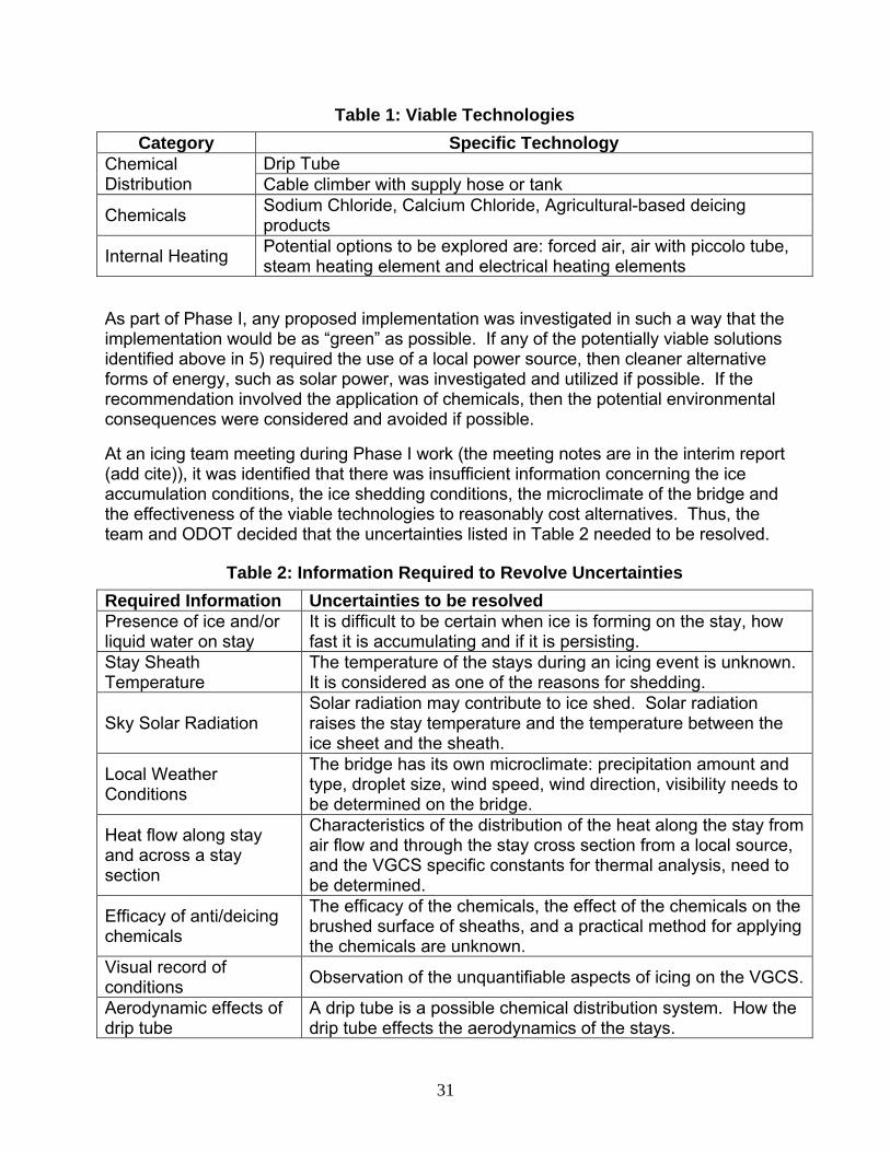
31

Table 1: Viable Technologies

Category Specific Technology Chemical Distribution

Drip Tube Cable climber with supply hose or tank

Chemicals Sodium Chloride, Calcium Chloride, Agricultural-based deicing products

Internal Heating Potential options to be explored are: forced air, air with piccolo tube, steam heating element and electrical heating elements

As part of Phase I, any proposed implementation was investigated in such a way that the implementation would be as “green” as possible. If any of the potentially viable solutions identified above in 5) required the use of a local power source, then cleaner alternative forms of energy, such as solar power, was investigated and utilized if possible. If the recommendation involved the application of chemicals, then the potential environmental consequences were considered and avoided if possible.

At an icing team meeting during Phase I work (the meeting notes are in the interim report (add cite)), it was identified that there was insufficient information concerning the ice accumulation conditions, the ice shedding conditions, the microclimate of the bridge and the effectiveness of the viable technologies to reasonably cost alternatives. Thus, the team and ODOT decided that the uncertainties listed in Table 2 needed to be resolved.

Table 2: Information Required to Revolve Uncertainties

Required Information Uncertainties to be resolved Presence of ice and/or liquid water on stay

It is difficult to be certain when ice is forming on the stay, how fast it is accumulating and if it is persisting.

Stay Sheath Temperature

The temperature of the stays during an icing event is unknown. It is considered as one of the reasons for shedding.

Sky Solar Radiation Solar radiation may contribute to ice shed. Solar radiation raises the stay temperature and the temperature between the ice sheet and the sheath.

Local Weather Conditions

The bridge has its own microclimate: precipitation amount and type, droplet size, wind speed, wind direction, visibility needs to be determined on the bridge.

Heat flow along stay and across a stay section

Characteristics of the distribution of the heat along the stay from air flow and through the stay cross section from a local source, and the VGCS specific constants for thermal analysis, need to be determined.

Efficacy of anti/deicing chemicals

The efficacy of the chemicals, the effect of the chemicals on the brushed surface of sheaths, and a practical method for applying the chemicals are unknown.

Visual record of conditions

Observation of the unquantifiable aspects of icing on the VGCS.

Aerodynamic effects of drip tube

A drip tube is a possible chemical distribution system. How the drip tube effects the aerodynamics of the stays.

32

In response to a request by ODOT at a project progress meeting to make the research immediately actionable by ODOT operations, a real-time icing condition monitor was developed. This monitoring system is referred to as the “icing dashboard” or simply “the dashboard” because the information necessary to support ODOT operations is presented on one simple visual display. The need to resolve the uncertainties in Table 2 and build on the capabilities of the dashboard led to a modification of Phase II research, which was initially focused on the implementation of viable technologies.

Final Phase II objectives were as follows:

1) Collect data to resolve uncertainties in Table 2. Some of the data may come from existing sensors while some of the data required new sensors (discussed later in this report), laboratory experiments and on-site observation. The collected information should be sufficient to allow accurate costing, resolve uncertainties to reduce the risk of deploying an icing strategy that does not work, and be useful for improving and updating the icing dashboard. The uncertainties to be resolved and the reason for resolving the uncertainty is listed in Table 2 above.

2) Make a recommendation on two to four viable active solutions. To make a decision on the viability on an active system, it is necessary to have a reasonable estimate of the cost and the practical implementation strategy.

3) Improve the icing dashboard. The dashboard tracks the icing events in a format that is easy to understand, is useful for managing icing incidents and archives data. Local condition data that is collected from the bridge will be used to increase algorithm intelligence and error handling. The improvements focused on the enhancement of the visual display, refinement of the accretion and shedding algorithms and incorporation of data for a local weather station on the bridge.

4) Development of an ice presence and state sensor. No suitable sensor exists. Therefore, development and field testing were undertaken.

5) Transition the dashboard board and local weather station to ODOT District 2 so that the functionality of the dashboard and the information from the icing sensors is available to the operators of the VGCS.

As with Phase I, any proposed implementation was to be as “green” as possible. If the recommended solution involved the application of chemicals, then the potential environmental consequences of the chemical waste stream were addressed and “green” alternatives for conventional chemicals were investigated and utilized.

The experimentation of the viable technologies will be thoroughly discussed in chapter 7 of this report. Through experimentation, no practical active or passive anti/deicing solution was ever identified. This ultimately led to a new overall objective, which was to improve the monitoring of icing events in order to provide ODOT with the best

33

information to manage their response to an icing event.

Section 2.4: Expert Team Approach to the Research

Because of the unique nature of the problem, the need for a quick response and the specialized nature of the icing knowledge required, the VGCS icing problem has been attacked with an expert team. The primary requirement was a team of researchers who are experts in ice and professionals familiar with the bridge. These are supplemented by team members who are expert in instrumentation, “green” energy and “green” chemistry. The team includes national expertise in icing from the U.S. Army Cold Regions Research and Engineering Laboratory and the NASA Glenn Icing Branch, expertise on the VGCS design and instrumentation, and experts in green technology. This team will address the unique features of the VGCS stays and provide recommendations to the Ohio Department of Transportation for the most practical and cost effective ice sensing, anti-icing and deicing systems for the VGCS.

An expert team was the best way to rapidly assess the state of the art. This approach allowed the research team to confirm that a practical solution for ice anti/deicing for the VGCS does not currently exists. The icing experts have identified the information that must be collected and understood to design an effective anti/deicing solution. The research team consists of the following members:

Jeff Baker, P.E., Independent consultant who was formerly the construction manager for VGCS, familiar with all aspects of VGCS construction and operation; experience with VGCS icing incidents.

Nabil Grace, Ph.D., College of Engineering Dean, University Distinguished Professor, Lawrence Technological University; Director, Center of Innovative Materials Research; director of the LTU Comprehensive Environmental Test Chamber which has large scale icing test capacity.

Michael Gramza, P.E., ODOT lead, District Construction Engineer for District 2, and former construction project manager of the VGCS.

Cyndee Gruden, P.E., Ph.D., Associate Professor of Civil Engineering, University of Toledo; environmental engineer with expertise in management of deicing waste streams.

Art Helmicki, Ph.D., Professor, Department of Electrical and Computer Engineering, University of Cincinnati; Director, Applied Systems Research Lab, a designer of the data collection system for the VGCS; expertise in sensor and signal processing.

Victor Hunt, Ph.D., Research Associate Professor, Department of Electrical and Computer Engineering, University of Cincinnati; expertise in bridge instrumentation, a designer of the existing VGCS instrumentation system.

Kathleen Jones, U.S. Army Cold Regions Research and Engineering Laboratory, Expertise; expertise in static and dynamic loads on structures due to atmospheric

34

icing; leader of freezing rain survey team; wrote ice load section for ASCE7 Standard, Minimum Design Loads for Buildings and Other Structures.

Richard Martinko, P.E., Director UT-University Transportation Center and Intermodal Transportation Institute; former deputy director of ODOT District 2, former assistant director of ODOT, and former ODOT project principal of all phases of the VCGS project.

Cyril Masiulaniec, Ph.D., Late Associate Professor, University of Toledo, Department of Mechanical, Industrial and Manufacturing Engineering; expertise in icing and thermodynamics.

Douglas Nims, Ph.D., P.E., PI of this project, Associate Professor of Civil Engineering, University of Toledo; instrumentation and structural study of the VGCS; management of engineering consulting and academic teams.

Tsun-Ming “Terry” Ng, Ph.D., Professor, University of Toledo, Department of Mechanical, Industrial and Manufacturing Engineering; expertise in icing and sensor. Currently, working on a study of icing on wind turbine blades..

Andrew Reehorst, NASA Glenn Icing branch; expertise in icing sensors; experience with ice accumulation and icing test facilities.

Charles Ryerson, Ph.D., U.S. Army Cold Regions Research and Engineering Laboratory, Manager of CRREL’s Icing Program, Deep; deep and broad experience with aircraft and structural icing. Familiar; familiar with icing test facilities. His 2009 study on off-shore facilities is similar to this VGCS study.

Thomas Stuart, Ph.D., Professor of Electrical Engineering University of Toledo; expert in power, PI of an ODOT funded research study of a solar installation near to provide power to the VGCS site.

Mario Vargas, Ph.D., NASA Glenn Icing Branch, lead. NASA Glenn has an icing wind tunnel and the researchers are familiar with the capabilities of icing test facilities.

Ted Zoli, S.E., Vice President of HNTB, expertise in icing; an extensive history of working with icing issues including testing structures on Mount Washington. Currently, he is engaged on two other cable stayed bridges with icing issues.

35

Table 3: Team Members Roles and Expertise

Team member Icing Expert

Local Knowledge

Green Expert

Brief Description of Primary Activity/Expertise

Jeff Baker X Former construction manager for VGCS, familiar with all aspects of VGCS construction and operation, experience with icing incidents.

Nabil Grace X Lawrence Technological University (LTU). Director of a unique low velocity wind/ freezing/icing/rain/load testing facility.

Mike Gramza X ODOT lead, former project manager of VGCS, able to provide input on ODOT operation needs.

Cyndee Gruden X University of Toledo. Expertise in management of de‐icing chemicals

Kathleen Jones X CRREL, national icing expert, leader in icing risk, member and former chair of ASCE‐7 committee on icing

Art Helmicki X University of Cincinnati. Instrumented VGCS, expertise in instrumentation and testing, support for implementation and testing costing

Victor Hunt X University of Cincinnati. Instrumented VGCS, expertise in instrumentation and testing, support for implementation and testing costing

Rich Martinko X University of Toledo. Understanding of ODOT operations, administrative support

Cy Masiulaniec X Late of the University of Toledo. Icing expertise, lead in performing thermal analyses and experiments.

Doug Nims X University of Toledo. Lead in administrative support. Instrumented VGCS, lead in developing background information for alternative, support for thermal calculations, lead in report writing and costing.

Terry Ng X University of Toledo. Icing expertise, lead in sensor development and experiments.

Andy Reehorst X NASA Glenn, icing sensor expert

Charles Ryerson X CRREL, national icing expert, recently completed oil platform study which is parallel to the present VGCS study, familiar with other test facilities nationally

Tom Stuart X University of Toledo. A lead in the design of the VCGS solar array, expertise in power management

Mario Vargas X NASA Glenn lead, aircraft icing expert, intimately familiar with test facilities at NASA Glenn and familiar with other test facilities nationally,

Ted Zoli X X HNTB. National icing expert, consultant on VGCS design and construction, experience with icing problems on existing bridges

36

Section 2.5: Benefits

The benefits accruing to the traveling public, operators of the VGCS, District 2 and ODOT in general include: benefits accruing to ODOT and D02 from the dashboard and database include.

1) Comprehensive review of existing active and passive technologies: With the support of team member Charles Ryerson and drawing extensively, on his studies of icing technology, all of the known anti/de-icing technologies were investigated. The included over 70 technologies and is described in the technology matrix summarized in this report and presented in detail in Belknap, 2011.

2) Comprehensive review of past weather events; Team member Kathy Jones reviewed the icing events in northwest Ohio for the past twenty years including the first four icing events on the bridge. Vehicles were damaged in at least two of the first four icing events. A summary of this work is presented in chapter 4.

3) Detailed study of the 2011 major icing event: This was the fifth major icing event on the bridge since its opening. The icing team was onsite from the initial rainfall through the icefall for the February 2011 major icing event. Pieces of ice several feet long and up to three-quarters of an inch thick fell. The bridge was closed for several hours. The team was able to capture video and images of the ice shedding that lead to increased understanding of the icing behavior. A summary of the study of the 2011 icing event is presented in chapter 4.

4) Ice accretion and shedding algorithms: The study of the past weather and icing events lead to quantitative guidelines concerning the weather conditions that made icing accretion and shedding likely. These guidelines form the core of the algorithms in the ice monitoring system implemented on the bridge.

5) Development and implementation of the dashboard: In response to ODOT’s request for a way to make the results of the research easily actionable by the operators of the bridge, a real-time monitoring system was implemented. Initially, the information from existing sensors on the bridge and in the surrounding region was feed into the ice accretion and shedding algorithms and the results displayed on a graphical user interface. This interface was design so it displayed information about the icing status of the bridge in a simple on screen format, much as the dashboard of a car is designed to put the information essential to the operation of the vehicle in a visually compact format. At present, the dashboard reflects information from the initial sensors as well as a bridge mounted weather station and camera as well as temperature sensors on the stay sheaths.

6) Design, installation and use of a local weather station on the bridge. When it was identified that the existing sensor system on the bridge and in the surrounding

37

regional area was not adequate to monitor the microclimate on the VGCS and icing conditions of the stays, it was decided that a suite of local sensors was required. The research team identified an array of commercially available sensors that could provide most of the required information. The team then procured the sensors. A weather tower with local sensors and a camera as well as stay as mounting brackets to attach thermistors directly to the sheath were designed and installed. The sensors were made operational and their data was incorporated into the dashboard.

7) Field and laboratory studies of anti-icing and de-icing technologies: Experiments on anti/deicing chemicals, anti-icing coating and anti/deicing application of a heating system were carried out on full scale sheath specimens at the icing experiment station and in the icing wind tunnel at the University of Toledo. These studies coupled with the literature review demonstrated that no existing technology was appropriate for anti/de-icing on the VGCS.

8) Development of an ice presence and state sensor: No commercial sensor for directly measuring the presence or state of ice on the sheath exists. An electrical resistance based sensor has been developed. The sensor detects the presence of ice and can detect the layer of water, which is a precursor to ice shedding between the ice and the sheath. This sensor has been tested in the icing wind tunnel and at the icing experiment station. It is ready for deployment.

9) Database: The dashboard collects a comprehensive set of from the regional and local sensors on the bridge. It records all the icing and shedding alerts, serves as a log for all the observations and has the capability of exporting and plotting the data. This provides a database than can be used for study of the icing behavior of the bridge.

10) Archive: In addition to the weather data, the dashboard serves as a repository of all references, reports, presentations and other documentation of this project. This allows convenient access to the information for ODOT and researchers.

Through this project, the safety of those crossing the bridge has improved, the understanding of icing events has advanced and a sensor array capable of ascertaining the state of icing on bridge has been installed.

Section 2.6: Chapter Summary

The overall goal of this research was to assist ODOT in implementing an icing management procedure for the VGCS.

The objectives to support this goal were to Evaluate the state of the art in anti/deicing technologies through literature review

and experimentation

38

Install sensors to understand the microclimate and icing on the bridge

Design a real-time monitoring system to track icing conditions on the bridge with a straightforward interface so information on the icing of the bridge was readily available to the bridge operators.

An expert team approach was followed. A team with local expertise in the VGCS and expertise in anti/decing was formed and carried out the tasks to achieve the objectives.

The objectives to support this goal were to Evaluate the state of the art in anti/deicing technologies through literature review

and experimentation

Install sensors to understand the microclimate and icing on the bridge

Design a real-time monitoring system to track icing conditions on the bridge with a straightforward interface so information on the icing of the bridge was readily available to the bridge operators.

The overall benefit is increased safety for the traveling public. The benefits of completing this project were:

Comprehensive review of existing active and passive technologies.

Identification that no existing technology was suitable for anti/deicing the VGCS.

Comprehensive review of past weather events. Detailed study of the 2011 major icing event. Ice accretion and shedding algorithms. Making real time icing information about the bridge available to the bridge

operators. Development and implementation of the dashboard. Design and installation of a local weather station on the bridge. Field and laboratory studies of anti-icing and de-icing technologies. Development of an ice presence and state sensor. Creation of an icing database. Creation of an information archive.

39

Chapter 3: Phase I Research

The research performed as well as the findings for Phase I of the VGCS project will be presented in this chapter. Phase I research included the VGCS’s stay sheath analysis, literary review, the completion of a technology matrix, and the identification of uncertainties as well as sensors that will resolve them. The research performed in Phase I allowed for better understanding of icing events that have occurred on the VGCS as well as viable ice protection technologies. During Phase I research, a number of uncertainties pertaining to the microclimate of the VGCS were identified. These uncertainties must be resolved in order to provide a practical anti/deicing technology and/or better monitoring of icing events, thus, several sensors were proposed.

The Phase II research is discussed in chapters 5 through 9.

Section 3.1: VGCS Sheaths

The stay sheaths of the VGCS are unique. Typical stay sheaths are high-density polyethylene (HDPE). However, for the VCGS, stainless steel sheaths were chosen over HDPE due to their low life cycle cost. The brushed stainless steel surface also is an aesthetic enhancement for this signature bridge. The reflection of the light off the stays provides a unique appearance and enhances the effect of the illuminated pylon. Some characteristics of the stays sheaths, such as being made of a 1/8 inch thick 316L stainless steel, a brushed finish, and having a larger than typical diameter, may contribute to the icing problem the VGCS is experiencing.

The stainless steel has a brushed finish. A Bendix Profilometer Peak Counter was used to determine the surface roughness on a sample piece of the VGCS sheath. The surface roughness could be a factor for ice clinging to the stays. After a team visit to the NASA Glen Icing Branch, it was determined that the sheath was roughly comparable to the smoothness of an aircraft, and therefore, did not facilitate icing. The test was run by The University of Toledo machine shop supervisor John Jaegly in the Material Science Lab room 1061 North Engineering. The machine uses a carbide tip moved across a surface. Table 4 shows readings taken across the grain of the brush finish and with the grain. Multiple readings were taken on multiple areas. Readings are in mirco-meters.

40

Table 4: Sheath Roughness Test Data

Across the Grain With the Grain Test Area

1 Test Area

2 Test Area

3

Test Area 1

Test Area 2

Test Area 3

1.269 1.212* 1.372* 0.228* 0.353* 0.470* 1.282 1.185* 1.347* 0.229 0.397* 0.485* 1.289 1.157 1.315* 0.231 0.405 0.507

1.146 1.345 0.218 0.409 0.503 1.150 1.374 0.206* 0.427 0.503 1.173* 1.367 0.381* 0.506* 1.171* 1.347* 0.390* 0.499* 1.373* 0.401*

Average Average Average Average Average Average 1.280 1.151 1.362 0.226 0.413 0.504

Avg. of 3 1.264 Avg. of 3 0.381

Note: * measurements are not included in the calculation of the average because the apparatus was being moved during the readings.

Section 3.2: Literature Review

Icing is a worldwide problem for large bridges and other industrial facilities in cold climates; therefore, a broad literature regarding both structures that have been affected and anti-icing/deicing technologies were reviewed. This section will first discuss known icing events that have been found in literature, then anti-icing/deicing technologies found in literature, and finally the technology matrix for the Veterans Glass City Skyway.

Section 3.2.1 Known Icing Problems on Other Bridges

Leonard P. Zakim Bunker Hill Bridge: This particular bridge is an A-type cable stayed bridge that crosses the Charles River in Boston, Massachusetts. In March of 2005, the Boston area experienced winter conditions that caused the cables sheaths of the Leonard P. Zakim Bunker Hill Bridge to ice. The ice then fell off of the stays in large sheets and onto the roadway below. Officials and design engineer considered this weather to be a “fluke,” thus, no technology was investigated (Daniel, 2005)

Penobscot Narrows Bridge: The Penobscot Narrows Bridge is an I-type cable stayed bridge that allows traffic to cross over the Penobscot River between Verona Island, ME and Prospect, ME (Penobscot Narrows Bridge and Observatory, 2014). The bridge was completed and opened in 2006 and experienced weather that caused icing for the first time in 2014. Due to the irregular occurrence of icing, the state DOT has taken an observation approach, thus, no technology is currently being investigated or deployed

41

(Gluckman, 2014)

Port Mann Bridge: The Port Mann Bridge is an A-type cable stayed bridge that allows traffic to cross the Fraser River in Vancouver, B.C.. The bridge was opened to traffic in 2012 and experienced winter conditions that resulted in the accretion and shedding of “wet” snow in December 2012. Several technologies have been investigated, which includes: heating of the stays, the use of water, the use of a helicopter, cable collars, coatings, chemicals, sensors, etc. Currently, cable collars have been deployed on several stays (Meiszner, 2013). They have been relatively successful, but at times they get stuck on their way down the stays. In addition to the cable collars, a dashboard has been set up in order to provide real-time conditions on the bridge.

Ravenel Bridge: The Ravenel Bridge is an A-type cable stayed bridge that connects Mt Pleasant, SC and peninsular downtown Charleston SC. In late January 2014, the bridge experienced weather that caused the cable stays to ice. Once the stays warmed up, ice began to shed causing damage to numerous vehicles passing below. There are reports of ice sheets as large as 8 to 10 feet falling from the cable sheaths (ABCNews4 WCIV-TV., 2014). Currently, there is not a technology deployed on this bridge.

Severn Bridge: consisting of the Aust Viaduct, Severn Bridge, Beachley Viaduct, and Wye Bridge; stretches from England to Wales. The bridge was closed for ice falling off the stay cable on two occasions, February 6, 2009 and December 22, 2009 (Severn Bridge, 2011).

Svinesund Bridge: The Svinesund Bridge connecting Norway and Sweden has an arc section of 188 meters (~617 feet). The single arc superstructure supports two-lane bridge decks on either side. To prevent ice formation on the arc during the winter, a temperature sensor controlled electric cable system was installed in the top section (Net Resources International, 2011).

Southern Quebec, western New Brunswick, and eastern Ontario were covered with thick ice in 1998 due to a significant ice storm. Bridges and tunnels were closed because of the weight concerns as well as falling from superstructures (Countryman Electric).

Uddevalla Bridge: The Uddevalla Bridge is an A-type cable stayed bridge located in Uddevalla, Sweden that crosses the Sunninge sound (Uddevalla Bridge in Sweden, 2012) .This bridge was opened to traffic in 2000 and has been experiencing frequent icing problems ever since (Bowers, 2014). Pulse electro-thermal de-icing (PETD) has been deployed on one cable and one pylon of the bridge for testing. Field testing, though successful, revealed a mechanical design flaw (Petrenko, 2011). This technology has been proven to be successful in icing conditions. In addition to PETD technology, the bridge consists of a large array of sensors that relay data back to a dashboard, which gives an early warning based on the microclimate of the bridge.

Section 3.2.2 Anti-Icing/Deicing Technologies found in literature

Chemicals are considered as both deicing and anti-icing technologies. They are widely available commercially and are used in several industries such as aviation, offshore oil industry, transportation departments, and marine structures. Chemicals have both dry

and wet strengthtechnolomost widchlorideconcernapplicati

Coating Coatingsto reducon the scoating 2011). Ahydrophdevelopewidely ufuselagea superh

F

Concerntheir per

New descold clim

Recentlya techniqinterfacefrom thesubcategvoltage tdielectric

application between ic

ogy, chemicdely used c, calcium ms regardingion persiste

is another s are a pas

ce the adhesurfaces (Ryin different

A new approobic materied a new csed for sev

e (Menini, 2hydrophobic

Figure 6: App

ns with coatrsistence th

signs, matemates to pre

y, innovativque to melte and then ue substrate. gories. Theto the ice/sc heating (R

ns. In anti-icce layer andcals are usuchemicals amagnesium g chemicalsence.

technologysive anti-icision strengyerson, 200materials woach of thisial which caoating with

veral industr2011). Figurc coating.

plication of S

tings are effrough the w

erials, and devent ice ac

e deicing tet ice. Theseuse externaElectrical t

ese techniquubstrate intRyerson, 20

cing, chemicd the substually used tore calcium acetate, ure

s are enviro

y that is an aing technoloth of ice to

08). In Kulinwith differens technologyauses wateice phobic

ries such asre 6 shows

Superhydrop

fficacy in prewinter.

details can bccumulation

echnologiese techniquesal forces, sutechniques ues includeterface, 2) p008).

42

cals are eitrate or prevo melt ice lachloride, mea, and agrnmental an

active subjeogy, which the surface

nich’s work,nt surface toy would be r to bead incharacteriss transmisswater drop

hobic Coatin

eventing of

be considern on their st

s have beens cause iceuch as gravhave devel

e the followipulse electr

her used tovent the forayers durin

magnesium ricultural band corrosion

ect of develmeans the

es and to pr ice repelle

opographiesthe develo

nto small drostics on alusion lines, alets on a su

ng on the Su

f ice formati

red for newtays.

n developee to de-bondvity or wind loped in thrng: 1) the a

ro-thermal d

o reduce themation of ic

ng or after icchloride, po

ased chemicn issues as

lopment aney are applierevent the f

ency of hydrs was evalupment of su

roplets. Menminum allo

aircraft wingurface whic

urface (Ryers

ion on the s

w cable-stay

d which used at the ice/drag, to rem

ree fundameapplication deicing, and

e adhesion ce. In deicince storms. Totassium cals. The mwell as

d testing. ed to surfacformation ofrophobic uated (Kulinuper nini has ys which is

gs, and ch is covere

son, 2008)

surfaces an

yed bridges

e electricity/substrate move the icental of a DC biad 3) ice

ng The

major

ces f ice

nich,

s

ed by

nd

s in

y as

ce

as

In the firconductoan oxygecontact astrengthremovinare typic

In pulse which mthe ice. deicing swith a hidegreesshort eletechnoloPetrenkoextensivof the prshows alayer.

rst techniquors. The Den and hydarea betwe. Figure 7 sg the ice. E

cally destroy

Figure 7: D

electro themelts the thin

Instead of systems, thigh current,

s warmer thectrical pulsogy is a papo presents

ve data fromromising feaa thin metal-

e, a small DDC current, tdrogen gas een the ice ashows the pExperimentyed due to

DC Bias Deic

ermal deicinnnest ice laheating the

he PETD ra low voltagan freezing

se is the souper which wthe PETD m

m laboratoryatures of th-foil heater

DC current through elemixture. Thand substrapresence ofts have demthe high cu

cing where E

ng (PETD), ayer and exte substrate pidly heats e pulse. Th

g melts a thiurce of the

was written bmethod, its y tests as wis method wwhich is us

43

is applied tectrolysis, ahe electrolyate, and conf bubbles inmonstrated urrents.

Electrolysis f

a thin film cternal energcontinuousthe ice-sub

he rapid risein layer of icenergy savby Petrenkotheory, res

well as sevewould be thsed in the ic

to the ice/suablates the iysis-driven ansequently n the interfaproof of co

forms Bubble

conductor isgy, wind or

sly as done btrate interfe of temperce and cauvings. The o (Petrenko

sults of comeral large-sche low energce/substrate

ubstrate intice into cavablation redreduces th

ace which hncept, but t

es (Ryerson,

s used in thgravity, is uby most ele

face for a ferature to onses ice debbest refere

o, 2011). In mputer simucale implemgy for deicie interface t

erface throvities filled wduces the

he adhesionelps in the conduct

, 2008)

he interfaceused to remectrothermaew secondsnly a few bonding. Thence of that

this paper,lations, and

mentations. ng. Figure to melt the

ugh with

n

tors

move al s

he

, d One 8 ice

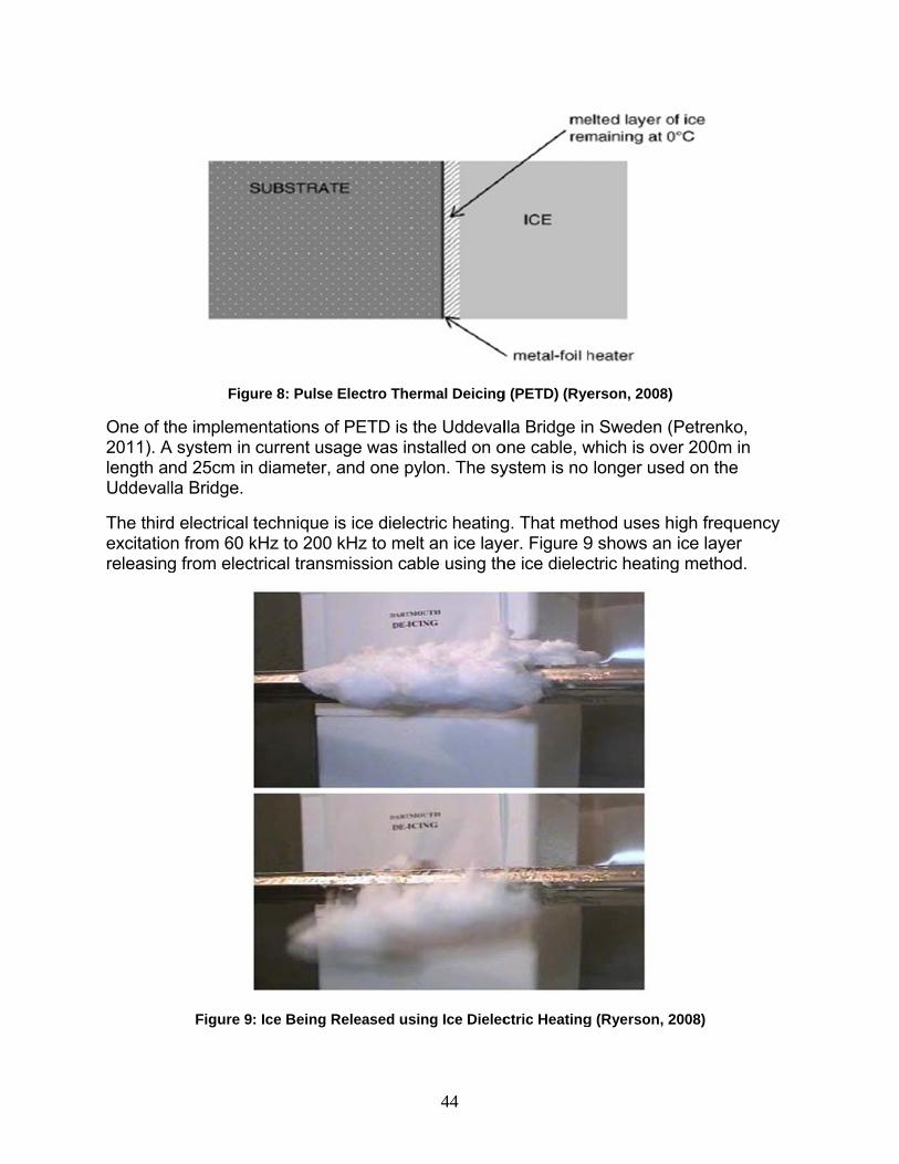
One of t2011). Alength aUddeval

The thirdexcitatioreleasing

Figu

he implemeA system in nd 25cm inlla Bridge.

d electrical on from 60 kg from elec

Figure 9

ure 8: Pulse

entations ofcurrent usa

n diameter,

technique ikHz to 200 ctrical transm

: Ice Being R

Electro Ther

f PETD is thage was insand one py

is ice dieleckHz to meltmission cab

Released usi

44

rmal Deicing

he Uddevalstalled on oylon. The sy

ctric heatingt an ice layeble using th

ng Ice Dielec

g (PETD) (Rye

lla Bridge inone cable, wystem is no

g. That meter. Figure 9

he ice dielec

ctric Heating

erson, 2008)

n Sweden (which is ove

longer use

thod uses h9 shows an ctric heating

g (Ryerson, 2

Petrenko, er 200m in ed on the

high frequenice layer

g method.

2008)

ncy

The nexexpulsivamplitudThe moswhich w

There arstructure

Electrothicing. In resistancconsiderthrough of this m

Figure 1head do

Figure

Another technoloindustryenergy t

Heated surfacesof ships factors savailable

xt technologve deicing sde and shorst applicablas designe

re several tes. The mos

hermal heaelectrotherce in wires red as an ethe wires is

method is th

0 shows anoors which is

10: Navy Ve

source of hogy is the a. The U.S. Ato blow war

pressure ws. The Navy(Ryerson, 2

such as: noe today tha

gy, which is ystems (EErt duration me design fod and deve

echnologiest applicabl

ting is usingrmal heatingsuch as nic

efficient heas convertede heating o

n applicatios used by t

ertical Launc

heat for deiutomobile wAir Force hrm air acros

washers andy considers 2008). The zzle size, fln when ste

consideredEDS). EEDSmechanicalor cable stayeloped by N

s which usele ones are

g electrical g, heating ochrome wireating systemd to heat, itsof automobi

n of heatinghe Navy.

h Systems w

cing and anwindshield das used jet

ss the wings

d steam nozthis technoefficiency o

low rate, wiam power w

45

d as new teS uses a vapulses to r

yed bridgesNASA Ames

e heat as ae electrother

resistance of substratees or carbo

m considerins use of elele rear wind

g cables to

with Electrica

nti-icing is hdefroster. Hengines m

s of iced air

zzles use hiology to be of a hydraund, and diswas commo

echnology, 2ariety of tecremove the s is an elects (Ryerson,

a method to rmal, hot ai

as a source occurs as on layers. Tng all of thectrical enerdows.

prevent ici

ally Heated D

hot air. The Hot air is us

mounted ontrcraft (Ryer

igh pressurviable and

ulic system stance. Thoon.

20 years oldchnologies t

ice from thtrically actu 2008).

deice or anir, and wate

ce in either da result elehough this

e energy corgy is costly

ng of hatch

Door Edges (

example osed widely ito trucks asrson, 2008)

re jets to reless expenis dependeough viable

d, is electroto create smhe substrateuated system

nti-ice er deicing.

deicing or aectrical method is

onducted y. An examp

hes and bul

(Ryerson, 20

of this n the aviatio

s a source o.

move ice frnsive for deient to varietye, steam is l

o-mall e. m

anti-

ple

k-

008)

on of

rom icing y of less

Another kind of rThere arprocess infrared (CRRELindustry

Millimeteof ice ontechnoloenergy a

The topiHowevelines, whdescript

technologyremote techre still additusing infraheaters to

L) facility. Fi.

Figure

Figure 12

er wave tecn surfaces. ogy is applicand heat th

c of atmosper, most of thich behaveion for vario

y, which is chnology whitional experred heatersdeice the digure 12 sh

11: Infrared

2: Aviation F

chnology is The ice natcable to anye surfaces

pheric icinghese studiee differentlyous phenom

considered ch heats thrimental ans (Koeing, 2door entrancows the ap

Heaters abov

acility using

another tecturally absoy situations(Ryerson, 2

g on cables es were cony than cablemena which

46

unique, is ihe objects thd analytica2011). Figuce at the Co

pplication of

ve the CRRE

Infrared Rad

chnology foorbs microws where wat2008).

has been snducted for e stay sheath include: rim

infrared deihrough absl needs to ure 11 showold Regionsf infrared de

EL Entrance

diant System

or deicing anwave energyter is availa

studied inteicing on to ths. Atmospme, fog, fre

icing. This msorption of iunderstand

ws the use os Researcheicing in the

(Ryerson, 20

m (Ryerson, 2

nd detectiny and heats

able to abso

ensively in thtransmissio

pheric icingeezing rain,

method is anfrared ene the deicing

of electric h Laboratorye aviation

008)

2008)

g the preses. That orb microwa

he past. on and pow

g is a gener and wet sn

a ergy. g

y

ence

ave

wer ral now.

47

An enormous amount of research has been conducted to understand the nature of the problem and to predict the icing load on the structure. In order to accomplish this goal, numerous ice and snow models have been developed in order to predict the thickness of ice and/or snow as well as the weight associated to the ice and/or snow. By being able to predict the aforementioned values, it becomes possible to examine the effect of this load on man-made structures.

Some scholars such as Makkonen (2010), Admirat (2008), Sakamoto (2000), Finstad (1988), and Nygaard (2013) have developed their own icing and snow models. Although they have developed different models, the significant parameters in the icing process are nearly the same for all of them. Additionally, all of the models follow the ISO standard equation for icing of structures (ISO12494 2001):

Where,

α : Collision efficiency - the ratio of the droplets that hit the cable to the total number of droplets in the windward side (Dubach et al., 2005);

α : sticking efficiency - the ratio of the droplets that stick on the cable to the total number of droplets that hit the cable (Dobesch et al., 2005);

α : Accretion efficiency - a representation of the amount of the droplets that will freeze to the total number of droplets that hit the surface;

A : Cross-sectional area perpendicular to object;

V : Particle impact speed perpendicular to object;

w : Water content [mass concentration of the ice particles].

The major difference between each model lies in the parameters of collision, sticking, and accretion efficiency; all of which depend on the event itself. Therefore, given the above equation, the factors that affect the formation of ice include: wind speed, precipitation type, precipitation amount or visibility (visibility can be substituted if the amount is unknown), and the size of the cable. In addition, some other factors that can be used for detecting the right conditions for an icing event are temperature and humidity.

In the future, the existing analytical studies could be advanced to address the torsional rigidity and geometry of the stays versus power lines. The stay specific models would be used primarily for forecasting ice accretion. The forecast weather data would be input in to the models and total accretion predicted. This forecasting of the ice accretion could be used to reduce the false alarms of the monitoring system.

Several anti/deicing technologies have been tested as passive or active solutions such as deicing or anti-icing. These solutions prevent or diminish the accumulation of ice on the surface of a cable, or in this case a stay sheath. Two examples of these technologies

include iin the indToledo. method accumu

Cable coas snowthem doby MeiszsignificaBridge toissues athe matedamagin

Section

The objesolutionsthe techthe cost

The techcategori

1

internal headoor icing tThese expethat was related ice on

Figure

ollars are aw and ice froown the stayzner (Meisz

ant amount oo remove “w

associated werial from thng the shea

n 3.3: Tech

ective of lites for VGCSnology, a dof each tec

hnology maes of techn

- Chemicaor agricu

ating systemunnel and teriments wi

ecently intron power line

13: Photonic

nother techom cable sty, ultimatelyzner, 2013)of weight. Twet” snow awith this teche stay, slidath.

hnology Ma

erature revieS. To reach

iscussion ochnology, a

atrix lists 75ologies inc

al and chemltural base

ms and the the outdoorill be discus

oduced by Ces; this is di

c Deicer for

hnology thatay sheathsy removing . They are This active and has beechnology incding over ice

atrix

ew was to athat goal, a

of its advantand the stat

potential telude:

mical distribuproducts a

48

super hydrr experimenssed in morCouture (20isplayed in

Deicing of P

t may be us. Cable cothe materiatypically intechnologyen relativelyclude gettine rather tha

assemble aa technologtages and dus was dev

echnologies

ution: Anti-nd practica

rophobic contation statire detail late011) utilizedFigure 13 b

Power Lines (

sed in ordellars work bal, as seen the shape y has been y successfu

ng stuck in tan removing

a comprehey matrix whdisadvantagveloped (Be

s in 13 diffe

icing/deicinal systems t

oatings, whion at the Uer in this red a photonicbelow.

(Couture, 20

r to removeby using grain the videoof a ring thused on thul at doing sthe processg ice, and th

ensive list ofhich has a dges, a rougelknap, 201

erent catego

ng chemicato distribute

ch were tesUniversity ofeport. Anothc deicer to m

11)

e material savity to forco in the artihat has a e Port Manso. Comms of removinhe potentia

f all potentidescription gh estimate 1, Ali 2013)

ories. The

ls such as se them.

sted f her melt

such ce cle

nn on ng l for

al of of ).

salt

49

2- Coatings: A layer applied to the surface of the sheath which prevents ice accretion on surfaces.

3- Design: Changing the shape of stay’s sheath to prevent ice accumulation.

4- Electrical deicing systems (electro-expulsive): Using repelling forces between conductors to produce an explosive force that ejects ice from the sheath.

5- Pneumatic expulsive deicing systems: That is the system which an inflatable boot covers the stays. When the boot is inflated, the ice cracks and falls down.

6- Heat: Use of thermal systems to prevent formation of ice or remove accumulated ice.

7- Infrared radiant heat: Use of radiant infrared heating to warm up the stays to prevent ice accumulation or remove accumulated ice.

8- Heating the ice-substrate interface: Applying heat directly to the interface between the ice and sheath. This reduces energy demand.

9- High-velocity water, air, or steam: Use of a high velocity stream of fluid to force the ice to fall off from stays.

10- Manual deicing methods: Chip or scrape ice off the stays.

11- Piezoelectric: Attach a piezoelectric actuator to the sheath surface to break the bond of ice to the stay causing shedding to occur.

12- Vibration or covers: Using vibration to break the ice-surface bond or covering the stays to prevent ice formation.

13- Ice detection: Sensors can monitor ice accumulation or detect the presence of ice.

Solving the icing problem of the VGCS is considered as applied research instead of basic research. Due to this fact, a technology selection meeting was held in June 2010. The notes for advantages and disadvantages of the technology matrix are available in a report which was submitted to ODOT, Innovation, Research and Implementation Section (Nims, 2010). Table 5 summarizes the most viable technologies which seem to apply for the icing problem of VGCS.

50

Table 5: Most Viable Solutions for the VGCS

Category Specific Technology

Chemicals

Sodium Chloride Agricultural Products Beet Heat Calcium Chloride

Coating Hydrobead

Heat

Internal Heating

- Forced air

- Air with piccolo tube

Section 3.4: Sensors on the VGCS

A key advance from phase I to phase II was the addition of a local weather station on the bridge. Prior to the 2012 – 2013 icing season, the VGCS had several existing sources of which data could be collected to better understand the local weather. The existing sources included several local airports as well as an ODOT Road/Runway Weather Information System (RWIS). In the research team meeting at the end of phase I, it was agreed that the existing sensor array was not adequate to capture the microclimate of the bridge, which is needed knowledge for understanding the VGCS icing events. To improve data collection, thermistors were added at several location on the bridge in the fall of 2012 and a weather tower was added in the summer of 2013. The detail of the new sensors is in chapter 6 and a discussion of the weather history from the sensors is in chapter 4.

Section 3.4.1: Sensors on the VGCS prior to the 2012 – 2013 Winter

The main existing local source was the ODOT RWIS site 142, which was installed on the VGCS. The RWIS station on the VGCS included the following sensors which were used to understand the weather conditions prior to the 2012-2013 icing season:

1. Linux RPU – RWIS Elite weather station platform. A full-feature weather station capable of sensing a variety of road weather conditions, gathering traffic data and activating roadside devices. This platform supports a full range of atmospheric sensors as well as pavement temperature and condition sensors.

2. Wireless Pavement Sensor X6 – Collects traffic and weather information. A self-contained, in-pavement sensor that utilizes Vehicle Magnetic Imaging

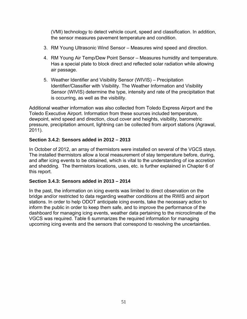
51

(VMI) technology to detect vehicle count, speed and classification. In addition, the sensor measures pavement temperature and condition.

3. RM Young Ultrasonic Wind Sensor – Measures wind speed and direction.

4. RM Young Air Temp/Dew Point Sensor – Measures humidity and temperature. Has a special plate to block direct and reflected solar radiation while allowing air passage.

5. Weather Identifier and Visibility Sensor (WIVIS) – Precipitation Identifier/Classifier with Visibility. The Weather Information and Visibility Sensor (WIVIS) determine the type, intensity and rate of the precipitation that is occurring, as well as the visibility.

Additional weather information was also collected from Toledo Express Airport and the Toledo Executive Airport. Information from these sources included temperature, dewpoint, wind speed and direction, cloud cover and heights, visibility, barometric pressure, precipitation amount, lightning can be collected from airport stations (Agrawal, 2011).

Section 3.4.2: Sensors added in 2012 – 2013

In October of 2012, an array of thermistors were installed on several of the VGCS stays. The installed thermistors allow a local measurement of stay temperature before, during, and after icing events to be obtained, which is vital to the understanding of ice accretion and shedding. The thermistors locations, uses, etc. is further explained in Chapter 6 of this report.

Section 3.4.3: Sensors added in 2013 – 2014

In the past, the information on icing events was limited to direct observation on the bridge and/or restricted to data regarding weather conditions at the RWIS and airport stations. In order to help ODOT anticipate icing events, take the necessary action to inform the public in order to keep them safe, and to improve the performance of the dashboard for managing icing events, weather data pertaining to the microclimate of the VGCS was required. Table 6 summarizes the required information for managing upcoming icing events and the sensors that correspond to resolving the uncertainties.

52

Table 6: Uncertainties that Needed Resolved and Corresponding Sensors

Required Information

Uncertainties that need to be resolved Sensor

Presence of Ice

It is difficult to be certain when ice accumulates on the stays except field observation. Ice thickness also triggers the criteria in falling conditions

Goodrich Ice Detector

Stay Temperature

The temperature of the VGCS stays during icing events is unknown. This temperature is considered as one of the reasons for falling conditions

Thermistors

Sky Solar Radiation

Solar radiation can cause the sheath surface temperatures to go above freezing even if the ambient temperature is below freezing. This can trigger shedding of ice off the stays

Sunshine Sensor

Local Weather Conditions

The VGCS has its own climate. Type and amount of precipitation, wind speed and direction need to be determined

LWS/ Rain Tipping Bucket

Visual records of icing conditions

Observation of the stays condition during icing events can be valuable

Camera

Taking the above information into consideration, several sensors were requested by the research team in order to reach the aforementioned objectives. The sensors requested and brief descriptions are as follows:

1. Goodrich Ice Detector: The Goodrich ice detector detects ice accumulation on an ultrasonic axially vibrating tube. It also measures precipitation transitions between liquid and solid condition (Goodrich, 2009). One of the unique features of this sensor is that it differentiates rain from freezing rain.

2. Leaf Wetness Sensor (LWS): Leaf wetness is a parameter which is used to describe the amount of dew or precipitation left on the surface. The LWS has a potential to detect if water is liquid or frozen.

3. Sunshine Sensor: It has been observed that solar radiation on the VGCS stays is a condition that can trigger ice shedding. This particular sensor measures both global and diffuse radiation as well as sunshine duration. The

53

sunshine sensor uses photodiodes with a computer generated shading pattern for measuring solar radiation (Delta-T Devices, 2002).

4. Electrically Heated Rain and Snow Sensor – R. M. Young’s Model 52202 (Campbell Scientific): It is an electrically heated precipitation gage which provides year-round measurement of rain and snow. It has been observed that ice accumulation and ice persistence depend on the rate and amount of precipitation. This sensor also uses a wind screen to minimize the effect of wind on the rain measurement.

5. Weatherproof Camera: The goal of having active weatherproof camera on the self-supporting instrumentation tower is to observe the unquantifiable aspect of icing events and track the performance of the dashboard. Reviewable visual record of icing events gives valuable information before, during, and after storms.

The aforementioned sensors were installed in the summer of 2013 with the weather tower. They provide critical information pertaining to the microclimate of the VGCS, thus, aiding in the understanding of icing events. A more detailed description may be found in Chapter 6 of this report.


This chapter thoroughly described phase I research. During phase I research, the VGCS stay sheaths were investigated, literature review regarding icing events on other structures as well as potential anti/deicing technologies was performed, a technology matrix to narrow down the numerous technologies to a few viable ones was constructed, and the history of sensor presence was given.

The VGCS stay sheaths are very unique when compared to the typical HDPE sheath. The unique features of the stay sheaths include being made of a 1/8 inch thick 316L stainless steel, a brushed surface, and a larger than typical diameter. The stay characteristics were chosen for aesthetic reasons and due to the low life cycle costs of stainless steel. Initially, the brushed surface of the sheaths was thought to potentially increase ice adhesion. After a team visit to the NASA Glen Icing Branch, it was determined that the sheath was roughly comparable to the smoothness of an aircraft, and therefore, did not facilitate icing. A roughness test was performed, which confirmed this belief.

Phase I literature review included icing events on structures, mostly bridges, from all around the world as well as potential anti/deicing technologies. The literature review showed that this is a relatively common problem for cable stayed bridges that are located in areas that experiences weather that gives rise to icing storms; this is described in detail in the following chapter. Additionally, it allowed for all potential technologies to be investigated and discussed in order to determine a viable technology to be used. However, it was determined that no such technology existed. Technologies that were investigated are as follows: chemicals, coatings, the application of a DC bias voltage to

54

the ice/substrate interface, pulse electro thermal deicing, ice dielectric heating, electro-expulsive deicing systems, electro thermal heat, hot air, water deicing, infrared deicing, millimeter wave technology, photonic deicer, and cable collars.

A technology matrix was then assembled in to gather, organize, and describe all of the technologies. This technology matrix included 75 potential technologies that were separated into 13 different categories. These technologies were then narrowed down to the most viable technologies at a technology selection meeting in June, 2010, which can be seen in Table 5 above. The entire technology matrix can be seen in Appendix X.

Additionally, at the technology selection meeting, it was determined that there was insufficient information concerning the ice accumulation conditions, the shedding conditions, the microclimate of the bridge and the effectiveness of the viable technologies. This ultimately led to the addition of sensors to the existing sensor array, which had been deemed inadequate. The existing array included the following sensors: Linux RPU – RWIS Elite weather station platform, Wireless Pavement Sensor X6, RM Young Ultrasonic Wind Sensor, RM Young Air Temp/Dew Point Sensor, Weather Identifier and Visibility Sensor, and a Tipping Bucket Rain Gauge. Thermistors were added prior to the 2012 – 2013 icing season and a Goodrich Ice Detector, Leaf Wetness Sensor, Sunshine Sensor, Electrically Heated Rain and Snow Sensor – RM Young’s Model 52202 (Campbell Scientific), and a weather proofing camera was added prior to the 2013-2014 icing season as part of the weather tower installation.

55

Chapter 4: Weather History, Modeling and Analysis

Section 4.1: Introduction

A brief look into the causes of ice storms as well as the history of icing events that have occurred on the VGCS will be presented in this chapter in order to provide a better understanding of icing events, nature of ice accretion and ice shedding, and what happens during ice storms. Since the VGCS was opened for service in July of 2007, there have been five major icing events that have occurred. Jones’ report describes the first four icing events and the weather conditions which preceded them (Jones, 2010). The last icing event, which occurred in February 2011, was directly observed by the research team. Since February 2011, there have been minor icing events that the Dashboard has collected data on. These minor icing events will also be discussed.

The weather history and the observed icing behavior described in this chapter serves as the basis for the ice accretion and shedding algorithms in the Dashboard.

Section 4.2: Description of the basic weather that gives rise to an ice storm

Freezing rain has been the cause of four of the five icing events on VGCS. A prolonged freezing rain event requires a layer of cold (below-freezing) air at ground level, warmer air aloft, a high pressure system to hold the cold air in the place, and precipitation. The duration of a freezing rain event depends on how long the high pressure stays in the place and variations in the thickness of the cold air layer at that location. For a major icing event in Toledo, typically, the warm air aloft comes from the Gulf of Mexico and the cold air originates in Canada. Liquid precipitation in the warm air layer (that may have fallen from the clouds above as snow) supercools as it falls through the cold air layer at the surface. If that layer is not too thick the supercooled drops remain liquid. These freezing rain drops are likely to freeze when they impact a cold surface, primarily because of convective and evaporative cooling, with some contribution from supercooling. If the surface cold air layer is thicker the drops might freeze as they fall, forming ice pellets. These particles of ice accumulate on the ground, but are likely to bounce or slide off the bridge stays. On the cold side of a freezing rain event the precipitation is likely to be falling as snow, and on the warm side the precipitation is plain rain. As an event like this evolves, the precipitation type at one location may change between rain, freezing rain, ice pellets, and snow, sometimes with different types of precipitation occurring at the same time.

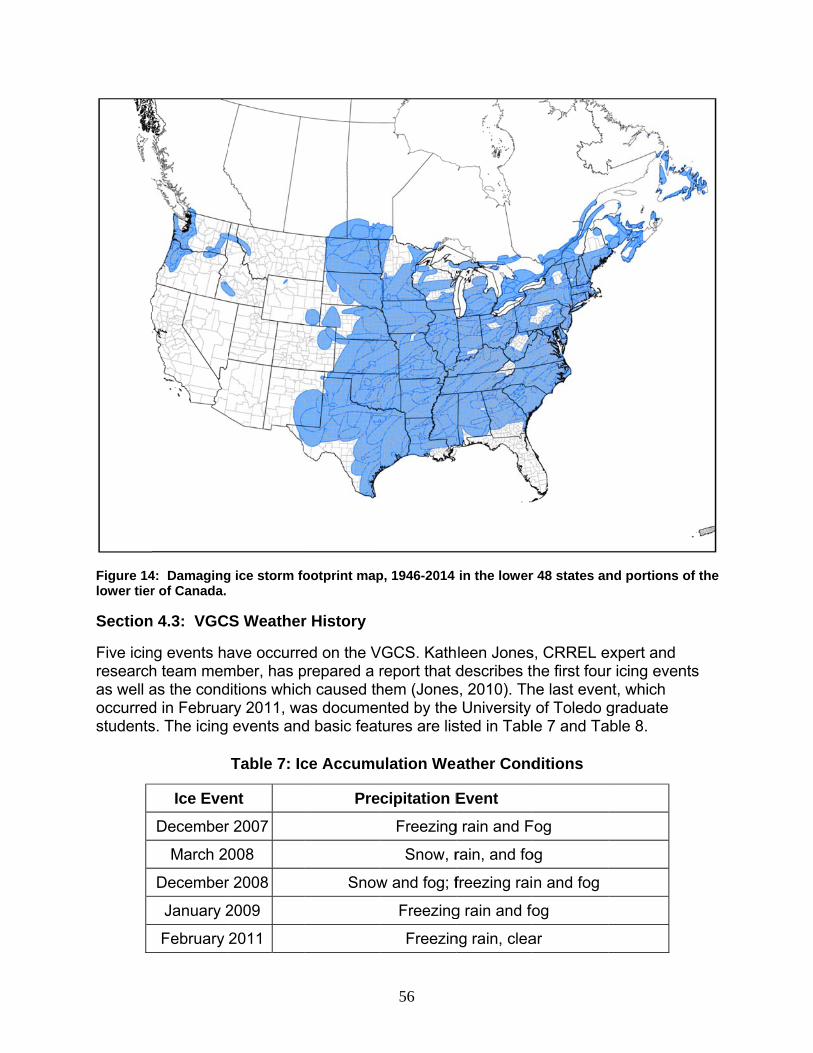
Figure 14lower tier

Section

Five icinresearchas well aoccurredstudents

4: Damagingr of Canada.

n 4.3: VGC

ng events hah team memas the condd in Februas. The icing

Ice Eve

December

March 2

December

January 2

February

g ice storm fo

S Weather

ave occurrember, has pditions whichry 2011, wa events and

Table 7: Ic

nt

r 2007

008

r 2008

2009

2011

ootprint map

r History

ed on the Vprepared a rh caused thas documend basic feat

ce Accumu

Pre

Snow

56

p, 1946-2014

VGCS. Kathreport that dhem (Jonesnted by thetures are lis

ulation We

cipitation E

Freezing

Snow, r

w and fog; f

Freezing

Freezin

in the lower

leen Jonesdescribes t

s, 2010). The University sted in Tabl

ather Cond

Event

g rain and F

rain, and fo

freezing rai

g rain and fo

ng rain, clea

r 48 states an

s, CRREL ehe first four

he last evenof Toledo g

le 7 and Ta

ditions

Fog

og

n and fog

og

ar

nd portions o

expert and r icing evennt, which graduate

able 8.

of the

nts

57

Table 8: Ice Falling Weather Conditions

Ice Event Ice Fall Weather

December 2007 Rain with temperature above freezing

March 2008 Sun with temperature above freezing

December 2008 Rain, gusty winds and temperatures above freezing

January 2009 Gusty winds, temperature above freezing

February 2011 Light wind, overcast, and temperature above freezing

It is also possible for wet snow to accumulate on the stays and cause an ice event. This wet snow, that includes both snowflakes and liquid water can accumulate on the stays. That means that an icing event can begin with the air temperature above freezing.

Icing on the cables of VGCS may also occur in supercooled clouds or fog. The Liquid water content of the fog is inversely proportional to visibility. Fog droplets, with typical diameters of a few 10s of microns, have essentially zero terminal velocity, so move only when they are carried by the wind. Therefore, in cloud icing is likely to be significant only in a thick fog and high winds.

To have a better understanding of icing events, nature of ice accretion and shedding, as well as what happens during ice storms, a brief summary and lessons learned from past icing events on the VGCS is presented below. Jones report describes the first four icing events and weather conditions that preceded them. The last icing event, February 2011, was captured and documented by the University of Toledo graduate students.

December 2007: The data from Toledo Express Airport and Metcalf Field indicated freezing rain and fog occurred on December 9 - 10, which is believed to have caused ice accretion on the stays. Rainfall with temperatures above freezing triggered the ice shedding from stays, which took place on December 12. Ice shedding resulted in the closure of two out of three lanes of traffic as well as damaged vehicles. (Jones, 2010)

March 2008: Weather data revealed that a snow and rain mixture with temperatures falling below freezing, concurrent with a fog, caused ice formation on the stays on the evening of March 27. The shedding of ice occurred in the afternoon of March 28. Clear

58

skies and air temperatures above freezing on March 28 were considered to be the shedding triggers. During the ice fall event, the center and left lanes in both directions had to be closed and at least one vehicle was damaged (Jones, 2010)

December 2008: On December 17, ice was first observed on the stays. Data gathered from Toledo Express Airport, Metcalf Field, and Toledo Blade indicated that freezing rain, snow, and fog were the conditions that caused ice accretion on the stays. On December 24, ice shedding occurred with temperatures above freezing and gusty winds. It should be noted that ice persisted on the stays for 7 days. Throughout this event, the left and center lanes were closed for 5 days, starting on December 19.

January 2009: Ice first was observed on January 3 and shedding occurred on January 13. The data from airport weather stations showed that freezing rain accompanied by fog caused ice accretion on the stays. Temperature rising above freezing and gusty winds on January 13 triggered the ice shedding from the stays. Note, the left lanes were closed until January 21, 2009. This could be due persistence of ice on the stays after the initial shedding event, which then melted over the next week (Jones, 2010).

February 2011: This icing event was observed and recorded from the time of ice accretion, which started on the evening of February 20, to the time in which ice shedding occurred, which began on the morning of February 24. This event will be given as a day by day account in order to provide a clear and better understanding of icing on the VGCS. Researchers were on the bridge regularly throughout the event to capture photographs and video as well as properly document the behaviors between the accreted ice and the VGCS stay sheath. A detailed description of this event is in Belknap, 2011. Photos and video from this event are permanently archived by ODOT Research.

The forecast for the night of February 20 was freezing rain, followed by a drop in temperature. On a local television station’s weather website (Storm Tracker 11, 2011), the forecasters predicted snow changing to freezing rain. The update for the overnight was scattered rain or freezing rain with additional ice accumulation. With low temperatures and precipitation, the conditions were conducive to ice accumulation.

The ice dashboard was monitored that night by the research team. RWIS Station 582016, located on the bridge, was tracked watching both the readouts from the dashboard and the cameras on the stays. At 9 pm, the dashboard ticker was reporting Y3, indicating that the conditions had been conducive to ice accumulation for 6 hour and visual observation should be made to ascertain if ice had accumulated. At 10:29 PM, a researcher and the ODOT shift supervisor visited the bridge and confirmed the presence of ice. With this confirmation, the dashboard was put on alert status. Figure 15 shows a screenshot of the ice dashboard on February 21. The “Record of the last 48 hours” at the bottom of the dashboard shows the progression of conditions from “clear” to “alert”.

Also, at the ODOstays. Arain andliquid wainch thicsmall iciside the Clear iceas glazesuper-coof meltin

The decice. Insid1 inch ththe westvisible. Fclose upthe distr

9 pm, ODOOT shift supt that time, the prevailater was click on top of cles and thstay was b

e with few ae ice. This isooled fog orng - rain wa

ck outside thde of the pahick. The icetern face. TFigure 16 sp of the ice aribution of th

Figure 15:

OT personnpervisor andthe air temling wind wnging to or the stay, ae ice was a

bare except air bubbles s opposed tr cloud drop

as running d

he parapet arapets on te covered t

The conditiohows an ovaccumulatinhe accumul

: Dashboard

el and resed the reseaperature waas from theblowing offbout ½ inch

about 1/2 infor occasiodeposited bto white rimps carried bdown and b

was coverethe medianthe eastern ons on the sverview of tng on the elated ice.

59

readout for

earchers obrchers returas 30° F an

e east. Rainf the stays.h thick on th thick on th

onal frozen by freezing

me ice with mby the wind lowing off t

ed with slus was an acface of the

stays appeahe ice accu

east face of

February 21

bserved ice rned to the nd the precin droplets wOn the stay

he east sidehe bottom o

rivulets. Clrain or free

more air bu(Ryerson, he icicles.

shy ice. Theccumulatione cable. Theared uniformumulation athe stay. F

, 2011

on the staybridge to o

ipitation wawere of avery checked, e of the sta

of the stay, aear ice wasezing drizzleubbles whic2011). The

e parapet hn of wet ice ere was littlem as far up and Figure 1Figure 18 is

ys. At 10:30observe the as cold blowrage size anthe ice was

ay, there weand on the s accumulae is referredh results fro

ere was no s

ad crusty wthat was 1/e to no ice othe stay as

17 shows a a schemat

0pm,

wing nd s 1/4

ere west

ating. d to om sign

wet /2 to on s ic of

Figure 1

Figure 1

6: Overview

7: Close up

of ice accret

of ice accret

60

ting on stay

ting on stay

at 10:29 PM

at 10:29 PM

Sunday eve

Sunday eve

ening

ning

Table 9 and Tole

Table 9 W

20/Feb/201RWIS DashboardToledo Me

On Febraccumufor the mthroughoalready at the in

The resethe backnear sta½ inch tvariationconsisteinspectio

compares tedo Metcalf

Weather Con

11 TemPrecSurfSurf

d Icingtcalf Tem

ruary 21, 20lated Sunda

morning andout the day on the stayside should

earch teamk span. Theay 6, which whick with clo

n in conditioent when vieon from ins

Figure 18:

the I-280 brf Field weat

nditions for

mp cip face face Temp g Condition

mp

011, Storm ay. They cad 3-5 inchesand accum

y and the neder. This all

stopped a ey chipped awas inspecosely space

ons along thewed near side the truc

Stay cable d

ridge RWISther reading

February 20

5-6 pm30° F None Wet 30° F

ns Clear 27° F

Tracker 11alled for an s of snow in

mulated on tew accumuows the ba

total of foua hole in the

cted from thed icicles ohe length ofstay 14 from

ck on from t

61

diagram with

S station weg.

0, 2011 (Ku

m 6-7 pm 30° F Rain Wet 30° F Y1 28° F

(2011) recadditional m

n the eveninthe stays. Alation in som

arrels to be q

r times, three ice to mee median. Tn the bottomf the bridgem the northhe south bo

h ice accumu

eather readi

mpf et. al, W

7-8 pm 830° F 3Rain RWet W30° F 3Y2 Y28° F 2

capped thatmix of snowng. The winA layer of snme areas. Oquickly reco

ee times oneasure thickThe ice on m. Then th

e, however, bound sideound side it

ulation

ing with the

Weather Un

8-9 pm 9-130° F 30°Rain RaWet We30° F 30°Y3 Ale28° F 26°

t 1/4” to 1/2w, freezing ntery mix annow was beODOT placonfigured to

n main spankness at thethe east sid

he team loothey appeae. Near stat was seen

e ice dashbo

nderground

10 pm 10-° F 30°

ain Raiet We° F 30°ert Ale° F 28°

” of ice rain, and slnd snow feletween the ced barrels o close lane

n and once e main spande was roug

oked for anyared to be ay 10 visualthat below

oard

, 2011)

11 pm F n t F rt F

eet l ice out es.

on n ghly y

l the

62

damper collar the ice appeared very thin or even possibly bare spots and above the damper collar ice appeared thicker with pronounced frozen rivulets. The team stopped one time on the back span near stay 8 where conditions were seen that roughly matched what was observed near stay 10.

The wind was from the east as it has been throughout the storm. Generally, on the east side, the ice appeared to be thicker than on the west side. The ODOT supervisor felt the coating on the east side was thicker than he had seen before. On the west side, there were some spots that appeared to have a very thin coat below the damper collar. Above the damper collar, ice was thicker and the frozen rivulets appeared more pronounced than on the east side.

The ice above the collar appeared uniform as high as it could be seen on both the east and west sides of the stay. However, it is impossible to discern anything more than gross icing further up than about mid-height.

On February 22, 2011, the temperature started at 15° F and climbed to 21° F by mid-afternoon then dropped to the teens again at sundown (Weather Underground, 2011). Although the air temperature was below 32° F, the sun was out and the solar radiation was 575 Watts/m^2 at 1:35 pm. At this time, the researchers observed liquid water under the ice on the stays and ice fall due to solar radiation seemed imminent. However, the ice did not fall when due to the solar radiation and the liquid water refroze at the end of the day.

The research team noted that water was dripping from the icicles on the bottom of the stays. There was ice covered snow in many spots along the stays. The ice cover was uniform from the bottom up to the pylon, as observed with binoculars. Cracking in the ice was observed on stay 4 and there was significant cracking of the ice at bottom of the sleeve. There was ice on the east face of the pylon glass, but there was not any ice on the west face of the pylon glass. ODOT moved the orange barrels out closing the inside lane.

Figures 19 and 20 portray the ice accumulation on the stays for February 22. The eastern face was coated and the western face was bare except for frozen rivulets.

Fig

On Febrtemperathe late Wind sp

Figur

gure 20: Froz

ruary 23, 20ature startinevening. No

peed reache

re 19: Ice Acc

zen Rivulets

001, the Weg at 19°F ino precipitated 9 mph m

cumulation u

and bare me

eather Unden the early mtion occurre

mostly South

63

up east side

etal on the w

erground (2morning aned and thereh to Southw

of stay Febr

west side of s

2011) archivnd rising throe was an ov

west (Weath

ruary 22, 201

stays Februa

ved the outrough the davercast skyher Undergr

1

ary 22, 2011

tside ay to 28° F y the entire round, 201

in day. 1).

The resereadingsthe ice athe mid-liquid wa

The temwas meameasuretemperathermoceasily inlittle resitemperaBecausetemperasurfacesThe tem32 F. TTable 10

earch teams and picturagain even -20’s. As theater was ob

mperature inasured throe surface teature was mcouple is apto the intersistance. Fig

ature of the e of the highature of the s, the infrare

mperature inhe lead for 0 shows the

Figure 21

continued res were takthough there team che

bserved und

the interstioughout theemperaturesmeasured wpproximatelystice. Some

gure 21 shostay surfach emissivitystay surfaced thermomdicated in tthe contac

e variation i

1: Thermoco

to monitor ken at interre was an ocked later i

der the ice.

ice, gap bee da. A Fluks and the teith a type Ky 0.1 inch inetimes the l

ows a measce, measurey of the brusce is overesmeter consisthe interstict thermocoun the tempe

ouple reading

64

the conditiorvals on theovercast skyn the day, t

tween the ike 561 InfraemperatureK contact thn diameter lead could s

surement beed with the shed alumi

stimated. In stently read

ce, measureuple can beerature in th

g between ic

ons on the be stays. Liquky and the athe ice was

ce accumured Thermo

es in the inteermocoupleand during slide in as feing taken. infrared thenum surfaclaboratory

d higher thaed by the coe seen insehe througho

ce and stay F

bridge. Temuid water wambient tems breaking o

ulation and someter waserstice. Thee. The leadthe day it w

far as 6-10 In Figure 2

ermometer,ce, it is likelytrials with r

an the actuaontact therm

erted into theout the day

February 23,

mperature was seen unmperatures off easily an

stay sheaths used to e interstice d of the contwould slide inches with

22, the indic is 27.0 F.y that the reflective al temperatmocouple, we interstice

y.

2011

nder in

nd

h,

tact

h cated

ture. was .

Time

8:15 am 8:50 am 9:20 am 9:30 am 9:45 am 12:15 pm 1:00 pm 1:00 pm 1:15 pm

2:55 pm

3:57 pm 5:23 pm

Even thothrough resultingincrease

Figure 22:

IntersticTempera24 F 24 F 24 F 28 F 26 F 30 F

31 F 32 F 35 F

32 F

32 F 31 F

ough the dathe clear g

g infrared rae in the tem

Thermocoup

Table 10:

ce ature

ay was overlaze ice. It t

adiation coumperature w

ple reading b

Interstice

Air Tempera21 F 21.9 F 21.9 F 21.9 F 21.9 F 24.1 F

24.1 F 24.1 F 24.1 F

25 F

27 F 27 F

rcast, the Uthen warmeuld not escaithin the int

65

between the

e Temperat

ature Sta

20N/A20151119

201918

20

2019

UV radiationed the surfaape the inteerstice. Due

ice and stay

ture Februa

ay Note

B No visiA No visiB B B Liquid B Liquid

pieces B B B Liquid

break fB Liquid

under tB B Liquid

break f

n penetratedace of the serstice, whice to this dra

y February 24

ary 23

ible liquid wible liquid w

water undewater unde of ice brok

water undefree easily. water that the ice refro

water undefree easily.

d the cloudsheath undech resulted amatic tem

4, 2011

water water

er ice er ice. Largeke free easi

er ice. Shee

had bled frooze on the

er ice. Shee

s and passer the ice. Tin a significperature

e ly.

ets

om stay.

ets

sed The cant

increaseportraysNote thetemperawater in under thstreams

At 5:23 pwater unsmall seprecariomade atdifferentat differe

e in the intes the fragilitye liquid wateature in the

the gap wahe ice was s.

Figure

pm stay 19nder most oection of iceously attacht ground levt. Figures 2ent stays an

rstice, a pay of the ice er on the suinterstice w

as in close csometimes

e 23: Crackin

B was examof the ice. Fe at the bottoed could ea

vel, so it is p5 and 26 arnd times.

atch of ice wwhen the in

urface of thewas 36 F. Tcontact withvisible and

ng in ice from

mined closeigure 24 shom of the sasily be dispossible thare schemat

66

was able to nterstice tee stay. TheThis seems h the overlawould run

m chipping aw

ely and it wahows the exstay was frolodged. All at the ice laics of the ic

be removemperature

e contact thea bit unrea

aying ice. Hout from un

way ice, Feb

as observextent of the ozen solidly the researc

ayer further ce buildup a

d easily. Fiis significanermocoupleasonable beHowever, wander the ice

bruary 23, 20

ed that therelayer of wa

y to the sheach observatup the stay

and liquid w

gure 23 ntly increase indicated ecause the ater movinge in small

11

e was liquidater. Only thath. Ice thistions were y was matewater observ

sed.

g

d he s

rially ved

Figure 224: Section w

Figure 25

where ice wa

5: Ice thickne

as chipped aw

ess measure

67

way to take t

ements on ba

temperature

ack stay 19 F

e readings Fe

February 23,

ebruary 23, 2

2011

2011

On Febrobservatwo junioThe ice conditionovercast

Traffic wlane as wactual lafilm timefallen. STemperawind. Thremaine

Table 11Field wetop. Figu

Table 112011)

24/Feb/2

RWIS 28 DashboToledo

Figure 26

ruary 24, 20tions. The ror researchfell in largens during tht sky, and li

was stoppedwell as off t

ane closure e. The ice coome ice remature at thehe south boed closed fo

1 compareseather readiure 28 show

: Weather c

2011

80 Bridge

oard Metcalf

6: Ice thickne

011 at 5amresearch teers to captuchunks, at

he sheddingight wind.

d at 9:30amthe bridge ais MOV042

ontinued tomained on

e time of theound lanes wor several ho

s the I-280 bings. Figurew the bridge

conditions f

Temp Precip Surface Surface TIcing ConTemp

ess measure

, a senior ream met on ure the ice t random intg event wer

m because pand into the201 with the

o fall until 11the pylon g

e ice fall wawere openeours becau

bridge RWIe 27 show ie deck after

for Februar

6

3NW

Temp 3nditions R

3

68

ements on ba

esearcher wthe bridge fall event. Atervals andre temperat

pieces weree Maumee Re last semi-1am. By thisglass as weas above freed before 1se of the ic

S with the ice accumur a majority

ry 24, 2011 (

6-7 am 7-

33° F 33None NoWet W33° F 33R1 R233° F 33

ack stay 19 F

was on the around 8am

At 8:40am, from randotures above

e falling closRiver. The v-truck drivins time, 80-9ll as on the

eezing (32° 1:30 am; th

ce on the py

ice dashbolation on thof the ice h

(Kumpf et. a

-8 am 8-9

3° F 34°one Non

Wet We3° F 34°2 R33° F 34°

February 23,

bridge makm. Camerathe ice fall

om stays. We freezing (

se to vehiclvideo foota

ng over the 90% of the stays closeF), overcas

he north bouylon.

ard and Tohe pylon glahad fallen o

al, Weather

9 am 9-10

° F 34° Fne None

et Wet ° F 34° F

R3 ° F 34° F

2011

king s were giveevent bega

Whether 32° F),

les in the ouge showingbridge at 5ice had alree to the pylst, and lighund lanes

ledo Metcaazing at the off.

r Undergrou

am 10-11am

F 34° Fe None

WetF 34° F

R3 F 34° F

en to an.

uter g the 5:28, eady on. t

alf very

und ,

1

F e

F

F

Figu

Figure 2

ure 27: Ice a

28: Ice on br

ccumulation

ridge deck af

69

n on pylon gl

fter 80-90% h

azing Februa

had shed, Fe

ary 24, 2011

ebruary 24, 22011

70

In summary, ice shed from the stay cables was confirmed. Videos from the ice fall event documented the size and fall pattern of the ice. Large rectangular pieces of ice from stays 20B-16B and 20A-16A, roughly, had pieces making it to the north bound outer lane of traffic and even completely off the bridge.

When the ice started accumulating on the stays Sunday night, barrels were set out one lane of traffic. As the days went by and the ice was predicted to fall, the barrels were moved out so that only one of three lanes of traffic could cross the bridge in the northbound direction and leaving two of the three lanes of traffic open in the southbound direction. This was decided because the ice had accreted most heavily on the eastern side of the stays and the typical wind direction throughout the persistence and shedding period was coming from the west. On Thursday February 24th, after about a half hour of ice falling, ODOT closed the lane behind stay 20B on the north bound side. Vehicles were routed off the bridge that could turn around. Once 80-90% of the ice was down, the vehicles remaining on the bridge were instructed to cross with caution. Once all the vehicles were off the bridge was closed until all the ice had fallen. The last ice to fall fell from the pylon glass in the early afternoon.

Figure 29 shows the weather for the week of February 20, 2011. Figures 30, 31, and 32 graph the solar radiation for February 22, 23, and 24, 2011, respectively.

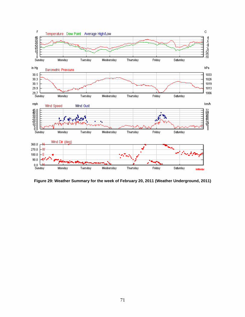
71

Figure 29: Weather Summary for the week of February 20, 2011 (Weather Underground, 2011)

72

Figure 30: Solar radiation counts February 22, 2011


0

100

200

300

400

500

600

700

12:0

0:00

AM

1:2

9:00

AM

3:0

0:00

AM

4:1

0:00

AM

5:4

2:00

AM

7:3

1:00

AM

9:1

3:00

AM

10:2

5:00

AM

11:4

8:00

AM

1:2

2:00

PM

2:4

6:00

PM

4:0

0:00

PM

5:3

3:00

PM

6:5

7:00

PM

8:1

0:00

PM

9:3

4:00

PM

10:5

4:00

PM

Wat

ts/m

^2

Time

Solar Radiation Feb. 22, 2011

Series1

0

50

100

150

200

250

12:0

0:00

AM

1:34

:00

AM

2:52

:00

AM

4:01

:00

AM

5:30

:00

AM

6:51

:00

AM

8:08

:00

AM

9:28

:00

AM

10:3

2:00

AM

12:0

2:00

PM

1:31

:00

PM

2:44

:00

PM

4:05

:00

PM

5:28

:00

PM

6:38

:00

PM

8:01

:00

PM

9:13

:00

PM

Wat

ts/m

^2

Time

Solar Radiation Feb. 23, 2011

Series1

73


Section 4.4: Lessons Learned from Previous Icing Events

There are several lessons to be learned from the five previous icing events. The first is how ice is accretes onto the stay sheaths. In all five events, accretion occurred in conditions where freezing rain and/or snow were present. These events are typically, followed by a sharp temperature drop and accompanied by fog. Additionally, it has been noted that in some events there is minimal precipitation, yet significant amounts of ice still accumulates, therefore it is possible that some of the ice that is accreted onto the stay sheaths comes from supercooled drizzle or cloud droplets (Jones, 2010).

Another lesson to be learned is how the ice sheds off of the stay sheaths. In four of the five events, shedding which cleared the ice off the stays occurred when the air temperature warmed to above freezing and was accompanied by gusty winds, clear skies or sunshine, and rain. The exception was the January 2009 event. Then ice shed intermittently and partially. Although, this was true for the last major icing event, which was the only to be directly observed and documented, it was learned that the temperature doesn’t necessarily need to be above freezing in order for shedding to occur. This is due to a greenhouse effect in the interstice between the ice layer and sheath surface. It was observed that considerable water flowed under the ice layer at temperatures in the mid-20’s. This effect caused ice to be removed easily, thus, displaying the possibility that shedding could potentially occur at temperatures below freezing (32 F).

The ice detector has proven to be sensitive and accurate for ice accretion. It may be possible to substitute

Solar Radiation feb. 24, 2011

050

100150200250300350

6:01

:00

AM

6:44

:00

AM

7:28

:00

AM

8:10

:00

AM

8:56

:00

AM

9:48

:00

AM

10:3

5:00

AM

11:1

7:00

AM

12:0

4:00

PM

12:3

7:00

PM

1:14

:00

PM

1:50

:00

PM

2:36

:00

PM

3:16

:00

PM

3:59

:00

PM

4:55

:00

PM

5:52

:00

PM

6:26

:00

PM

Time

Wat

ts/m

^

Series1

74

Section 4.5: Analysis

The common weather conditions prior to the previous ice events on the bridge led to the development of criteria to use when checking for icing event conditions.

Weather conditions (for at least 6 hours) that would likely cause Ice Accumulation:

1. Precipitation with air temperature at the bridge below 32o F, or 2. Fog with air temperature at the bridge below 32o F, or 3. Snow with air temperature at the bridge above 32o F.

Weather conditions that would likely cause Ice Fall:

1. Air temperature above 32o F (warm air), or 2. Clear sky during daylight (solar radiation).

In order to automate the process of predicting ice fall events, an algorithm was developed based upon the above criteria to evaluate weather data. The weather data collected consists of RWIS measurements and METAR data from the local airports. Taking these criteria and the available data into account, a specific set of criteria was developed for Ice Accumulation and Ice Fall (Tables 12 and 13).

Table 12: Ice Accumulation Criteria Source Condition Description

METAR or RWIS

Freezing Rain

(Air Temp. <= 32o F & Precipitation type is Rain) OR (Precipitation type is Freezing Rain)

METAR Freezing Fog

Air Temp. <= 32o F & Precipitation type is Fog

METAR or RWIS

Wet Snow Air Temp. > 32o F & Precipitation type is Snow

Table 13: Ice Fall Criteria Source

Condition

Description

METAR Warm Air Air Temp. >= 32o F METAR or RWIS

Clear Sky Condition type is Clear

The data sources used, including the secondary sources used for redundancy, are:

METAR Data Sources

1. http://www.wunderground.com/history/airport/KTOL/2011/05/13/DailyHistory.html?format=1

2. http://www.wunderground.com/history/airport/KTDZ/2011/05/13/DailyHistory.html?format=1

75

3. http://weather.noaa.gov/weather/current/KTOL.html 4. http://weather.noaa.gov/weather/current/KTDZ.html

RWIS Data Source

1. ftp://ftp.dot.state.oh.us/pub/doit/ssi_rwis/ 2. http://www.buckeyetraffic.org/reporting/RWIS/results.aspx

The RWIS stations report only four precipitation types (Rain, Snow, Fog, None/Other) while the METAR stations report more than 30 types, many of which are similar and could be grouped into the four RWIS types. A similar grouping is applied to the METAR data for the Ice Fall criteria. The only available metric for sky cover is from the METAR data. This metric had several values, four of which are used to classify the sky cover as “Clear”, with all other values grouped as “Not Clear”.

Several assumptions guided the design of the dashboard. The assumptions below are based on Kathleen Jones’ report (Jones 2010a), discussions with research team members Kathleen Jones and Jeff Baker and Mike Madry, ODOT Northwood Outpost, concerning the icing events on the VGCS. The assumptions are rough guidelines. There will be exceptions to the assumptions.

Assumptions:

Ice accumulates in a discrete time period and does not fall during that period.

The threshold of concern is radial ice accumulation of ¼”

It takes a long event (roughly 12 hours or more) for ice to accumulate.

If the sky is overcast and the temperature is less then 32°F, the stay sheath temperature after the icing event remains below freezing. (Note: On Tuesday February 23, 2011 this assumption was revealed to be flawed.)

Ice can accumulate on the stays from fog or precipitation other than freezing rain, e.g., wet snow accumulations can lead to ice accumulation on the stays.

Air temperature can be used as a reasonable approximation for stay sheath temperature.

Wind by itself does not trigger an ice fall.

Previously accumulated ice falls when either of these conditions occur

o The stay sheath temperature rises above freezing.

o If the sky is clear, sunlight could trigger the ice fall at temperatures below freezing.

76


This chapter described the weather that gives rise to ice storms, the VGCS’s weather history including previous icing events, lessons learned from those previous icing events, and accretion and shedding algorithms.

The weather system most often associated with major icing is warm air from the Gulf of Mexico overriding cold air from Canada. This leads to liquid water falling on a cold surface. However, other conditions and weather systems have also lead to ice accretion. Historically, roughly two icing events occur each year. The last major icing event on the VGCS was in 2011. Once the ice accretes, it persists until shedding conditions occur.

Temperatures above 32 and/or solar radiation cause ice fall. The ice fall in four of the five previous events was accompanied by temperatures rising above 32. If the solar radiation level is high enough, ice can shed. In February of 2011, copious amounts of water flowing beneath the ice were observed when the outside temperature was several degrees below freezing. This layer of water below the ice is a precursor to ice shedding. There is a greenhouse effect that occurs when the solar radiation passes through the ice and heat is trapped between the sheath and the ice. Ice accretion and shedding do not occur simultaneously.

The findings from the weather study and observation include: The VGCS is not a special icing structure which accretes ice at a rate different

from the surrounding structures. The hazard arises because the aerodynamic ice sheets from the stays can fall on vehicles crossing the bridge.

Ice can come directly from precipitation or supercooled drizzle or fog. The development of ice accretion and shedding rules

77

Chapter 5: Development of the VGCS Dashboard and Initial Dashboard Results


When no existing ice prevention or removal technology appeared to be practical and/or economical for the VGCS, ODOT elected to proceed with a monitoring system to assist them in managing icing incidents.

Literature review and contact with experts revealed no existing monitoring technology. Therefore, a novel monitoring system was designed, implemented and executed which is the first step in finding a long-term solution. The goal was to integrate a complex set of data and produce a concise graphic interface that put actionable information at the bridge operator’s fingers tips. Much as a dashboard puts key information about automobile operation in the visual field of a driver. A dashboard was developed that helps in monitoring ice events and other related parameters at VGCS for continuous flow of weather data. It also helps in getting actionable information in the hands of those who must anticipate and respond to an icing event. The working of the initial dashboard was based on a set of newly designed algorithms, with the following key features:

Dashboard is only using existing sensors, thus, there is no additional cost of instrumentation or installation. Many are maintained by others.

An existing suite of local weather stations is utilized to form a virtual 2-D area or network of weather data in order to detect approaching weather conditions or patterns conducive to ice accretion and/or shedding.

The dashboard works on a set of algorithms, which is the result of an extensive study of the causes and patterns of icing.

The solution used in the dashboard is very flexible and can be modified as per user’s requirements.

The solution can be used for any location/site and not just restricted to VGCS. This chapter explains the working, algorithm, user interface and performance of the dashboard in detail. It can also be seen that since designing and implementing a practical solution will take several winters, the current solution needs the regular attention of the user (i.e., Ohio Department of Transportation) at several parts of the solution for a successful implementation.

The primary objective of this aspect of the larger project was to leverage existing weather data from sources available on the web in order to develop a virtual instrument. This virtual instrument allows weather researchers, infrastructure researchers, and transportation personnel all to monitor for potential icing events from any Internet connected device. Listed below is the list of tasks for this phase of the project:

Add weather data to existing VGCS web interface and database for possible use in algorithms below.

Develop a “check engine” light (e.g., green (no ice), yellow (ice, but no shedding), red (ice with possibility of shedding) that responds to the algorithm and sends out corresponding alerts to a list of ODOT’s choosing.

78

Develop a reporting function that will allow ODOT to: o Verify that alerts are responded to o Declare an icing event o Capture time stamp and observation notes/comments

Develop database of ground truth field data collected during actual icing events to compare against Dashboard performance.

Develop export function for historical data archived on the VGCS weather website.

Run calibration studies based on historical/archived/ground truth data and characterize probabilities of false alarms and missed detections (i.e., false positives and false negatives).

To accomplish this, a dashboard was developed which included the virtual instrument to deliver the right information based on the task list mentioned above. The dashboard also provides a rich toolset for more detailed monitoring and assessment based on regular collection and storage of weather data from multiple sources. In addition the dashboard provides a way to interact with all data collected by location on a map and plotting the different types of measurements over time.

Icing is a complex problem, and no solution has been designed to remedy it, therefore, to design an online monitoring system of continuous weather data is especially helpful, a divide and conquer approach was followed. This approach is explained in Figure 33 by a process flow diagram. Following are the major steps followed:

1. Icing Experts: First step is to get necessary information from icing experts that includes researchers in Cold Region Research and Engineering laboratory (CRREL) and ODOT. The information is then analyzed to determine the icing criteria for all the three stages in icing namely ice accumulation, ice persistence, and ice shedding.

2. Data Collection: This is a crucial phase and involves three steps: Realizing reliable weather sources Choosing appropriate weather parameters that need to be considered in the

algorithm design, since different sensor system measure different weather parameters.

Collecting weather data from different sources and make it available to use 3. Data Processing: This phase involves the main analysis and design; it is explained

through a flowchart below. The main steps are: Ice accumulation checks for the last hour, get the results and store in the

database Ice accumulation check for the last few hours to determine ice persistence In case ice is detected, manual check should be done followed by reporting to

dashboard Ice shedding checks for the last one-hour, get the results and store in the

database Ice shedding check for the last few hours to determine ice persistence

4. User Interface: The final step is the design of a simple user interface that lets the user to check icing status at just one-click. It also provides lot of useful data to researchers pertaining to ice events.

Overview

Section explainsfor ice e

Section for one-h

Section Section

Section

Section events.

w of this ch

2 explains s about diffevent determ

3 explains hour time.

4 explains 3.

5 explains

6 deals wit

F

hapter:

different crerent types mination.

the algorith

the algorith

the feature

th the perfo

Figure 33: Pr

riteria for iceof weather

hm used to

hm for calcu

es and desig

ormance tes

79

rocess Flow

e accumular stations an

determine

ulating likel

gn of the da

sting of das

Diagram

ation and icnd the para

ice accumu

ihood of ici

ashboard.

shboard for

ce sheddingameters tha

ulation and

ing using th

the past an

g. It also at are impor

ice sheddi

he results fr

nd recent ic

rtant

ng

rom

cing

80

Section 5.2: Weather Data

Section 5.2.1: Introduction

To accomplish the objectives mentioned in the Section above, the first step is to gather information regarding weather conditions pertinent to icing. Based on statistical analysis of meteorological data [Savadjiev], there are various meteorological variables that affect the process of ice accretion and ice shedding. Extensive analysis was done on 57 icing events, which occurred in the period between February 1998 and January 2000 at the Mont Bélair in Quebec, Canada. Savadjiev also declared that freezing rain is the most important reason behind ice accretion.

K.F. Jones performed a pervasive analysis of the icing events’ that occurred in Toledo between 2000 and 2010, and found some of the common properties that were persistent during each ice events. Some of the results taken from Jones’ work are listed below:

Ice accumulation occurred in both freezing rain and snow, both accompanied by fog.

Ice shedding occurs when the air temperature warms to above freezing, which may be accompanied by rain, sunshine, or gusty winds.

Freezing rain was associated with ice accumulation on the Skyway stays in three of the four ice events.

The results from Savadjiev and Jones led to the development of criteria to use when evaluating for ice events conditions:

Criteria that would likely cause Ice Accumulation:

1. Freezing Rain: Precipitation with air temperature below 32oF. 2. Freezing Fog: Fog with air temperature below 32oF. 3. Wet Snow: Snow with air temperature above 32oF.

Criteria that would likely cause ice fall are as follows:

1. Warm Air: Air Temperature above 32oF. 2. Solar Radiation: Clear sky during daylight.

Section 5.2.2: Data Sources

To capture the icing criterions mentioned above, meteorological data are taken from different weather sources. They are:

(1) Road Weather Information System (RWIS): RWIS can be defined as a combination of technologies that uses historic and current climatologically data to develop road and weather information (for example, now casts and forecasts) to aid in roadway-related decision making. The three main elements of RWIS are:

Environmental sensor system (ESS) technology to collect data. Models and other advanced processing systems to develop forecasts and tailor

the information into an easily understood format.

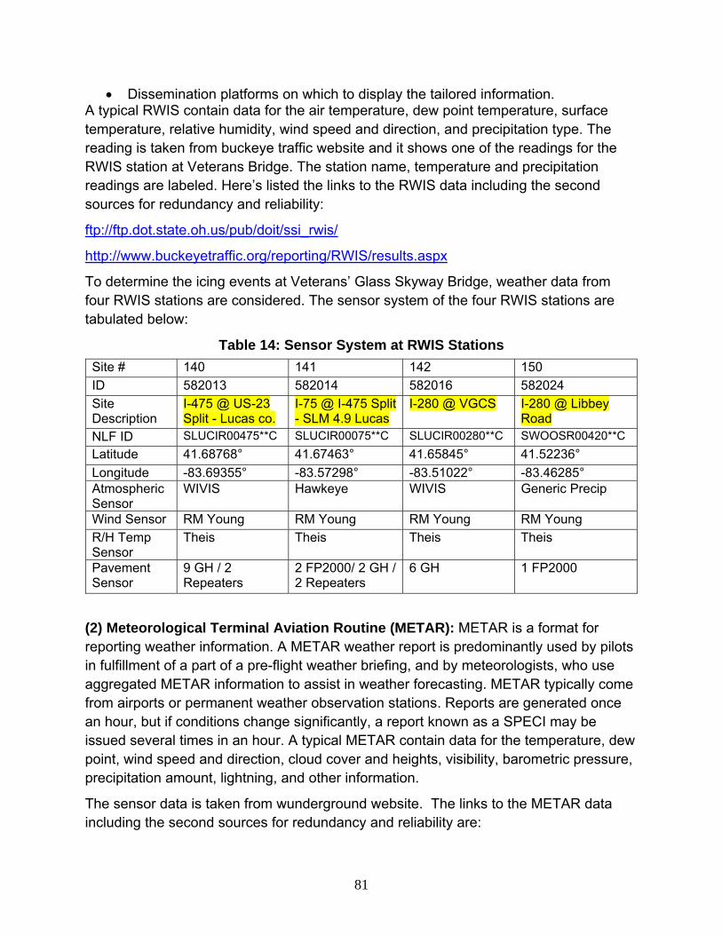
81

Dissemination platforms on which to display the tailored information. A typical RWIS contain data for the air temperature, dew point temperature, surface temperature, relative humidity, wind speed and direction, and precipitation type. The reading is taken from buckeye traffic website and it shows one of the readings for the RWIS station at Veterans Bridge. The station name, temperature and precipitation readings are labeled. Here’s listed the links to the RWIS data including the second sources for redundancy and reliability:

ftp://ftp.dot.state.oh.us/pub/doit/ssi_rwis/

http://www.buckeyetraffic.org/reporting/RWIS/results.aspx

To determine the icing events at Veterans’ Glass Skyway Bridge, weather data from four RWIS stations are considered. The sensor system of the four RWIS stations are tabulated below:

Table 14: Sensor System at RWIS Stations

Site # 140 141 142 150

ID 582013 582014 582016 582024

Site Description

I-475 @ US-23 Split - Lucas co.

I-75 @ I-475 Split - SLM 4.9 Lucas

I-280 @ VGCS I-280 @ Libbey Road

NLF ID SLUCIR00475**C SLUCIR00075**C SLUCIR00280**C SWOOSR00420**C

Latitude 41.68768° 41.67463° 41.65845° 41.52236°

Longitude -83.69355° -83.57298° -83.51022° -83.46285° Atmospheric Sensor

WIVIS Hawkeye WIVIS Generic Precip

Wind Sensor RM Young RM Young RM Young RM Young

R/H Temp Sensor

Theis Theis Theis Theis

Pavement Sensor

9 GH / 2 Repeaters

2 FP2000/ 2 GH / 2 Repeaters

6 GH 1 FP2000

(2) Meteorological Terminal Aviation Routine (METAR): METAR is a format for reporting weather information. A METAR weather report is predominantly used by pilots in fulfillment of a part of a pre-flight weather briefing, and by meteorologists, who use aggregated METAR information to assist in weather forecasting. METAR typically come from airports or permanent weather observation stations. Reports are generated once an hour, but if conditions change significantly, a report known as a SPECI may be issued several times in an hour. A typical METAR contain data for the temperature, dew point, wind speed and direction, cloud cover and heights, visibility, barometric pressure, precipitation amount, lightning, and other information.

The sensor data is taken from wunderground website. The links to the METAR data including the second sources for redundancy and reliability are:

82

http://weather.noaa.gov/index.html

http://www.wunderground.com/history/airport

To determine the icing events at Veterans’ Glass Skyway Bridge, weather data from two Airports are considered. The sensor system of the two airports are tabulated below:

Table 15: Airport Information

Site # Toledo Express Airport Metcalf Field Airport

ID KTOL KTDZ

Latitude Degree 41.5886° 41.5631°

Longitude Degree -83.8014° -83.4764°

Observing Program

LAND SURFACE COOP AB ASOS ASOS-NWS

LAND SURFACE ASOS ASOS-FAA

Source of the above data is: http://www.faa.gov/air_traffic/weather/asos/?state=OH

The observing system in both the airports are of the type Automated Surface Observing Systems (ASOS). It is a joint effort of the National Weather Service (NWS), the Federal Aviation Administration (FAA), and the Department of Defense (DOD). The ASOS system serves as the nation's primary surface weather observing network and is designed to support weather forecast activities and aviation operations and, at the same time, support the needs of the meteorological, hydrological, and climatological research communities. The basic weather elements measured by ASOS observing systems are:

Sky condition: cloud height and amount (clear, scattered, broken, overcast) up to 12,000 feet

Visibility (to at least 10 statute miles) Basic present weather information: type and intensity for rain, snow, and freezing

rain Obstructions to vision: fog, haze Pressure: sea-level pressure, altimeter setting Ambient temperature, dew point temperature Wind: direction, speed and character (gusts, squalls) Precipitation accumulation

Source of the above data is: http://www.weather.gov/ost/asostech.html

As explained above the implemented ice monitoring system for the Veterans’ Bridge uses a total of six weather stations which is tabulated below:

1111TM

There arpooling w

(1) Distashown inof the ex

(2) Reliaobtainedairports weather

Section

The weaexplaine

Ta

Weat

140-IR 475 @141-IR 75 @142-I-280 @150-I-280 @Toledo ExpreMetcalf Field

re a coupleweather da

Figur

ance from tn the table xperimenta

ability: The d via Weathare run by

r service in

n 5.2.3: Dat

ather data ced above. S

able 16: Dis

ther Station

@ US 23 Sp@ SLM 4.9 47@ VGCS @ Libbey Roa

ess Airport d Airport

e of reasonsata for the ic

re 34: Map Sh

he site: Theabove. It shl site. Figur

local weathher Undergrthe Nationathe country

ta Classific

collected coSince the tw

stances of

n St

plit RW75 Split RW

RWad RW

AiAi

s behind chce monitori

howing Dista

e distanceshows that are 34 is a m

her stationsround, whical Weather y.

cation

onsisted of wo weather

83

Weather S

tation Type

WIS WIS WIS WIS irport irport

hoosing the ng system,

ances of Wea

s of the weaall the chose

map showing

s are operatch would haService (N

RWIS meastations me

Stations fro

e Arial Vetera6.4 m11.2 m0 mile10.2 m12.2 m10.3 m

above six some of th

ather Station

ather stationen stationsg the weath

ted by varioave varying

NWS), which

asurementseasure a va

om VGCS

Distance froans iles miles es miles miles miles

weather stahem are list

ns from VGC

ns from thes are within her stations

ous sourcesg levels of rh is the mo

s and METAariety of we

om

ations for ted below:

CS

e Veterans’ 12 miles ra

s.

s and data eliability. T

ost dependa

AR data as eather

are adius

is The able

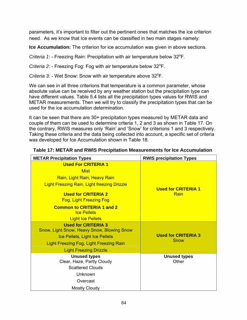
84

parameters, it’s important to filter out the pertinent ones that matches the ice criterion need. As we know that Ice events can be classified in two main stages namely:

Ice Accumulation: The criterion for ice accumulation was given in above sections.

Criteria 1: - Freezing Rain: Precipitation with air temperature below 32oF.

Criteria 2: - Freezing Fog: Fog with air temperature below 32oF.

Criteria 3: - Wet Snow: Snow with air temperature above 32oF.

We can see in all three criterions that temperature is a common parameter, whose absolute value can be received by any weather station but the precipitation type can have different values. Table 5.4 lists all the precipitation types values for RWIS and METAR measurements. Then we will try to classify the precipitation types that can be used for the ice accumulation determination.

It can be seen that there are 30+ precipitation types measured by METAR data and couple of them can be used to determine criteria 1, 2 and 3 as shown in Table 17. On the contrary, RWIS measures only ‘Rain’ and ‘Snow’ for criterions 1 and 3 respectively. Taking these criteria and the data being collected into account, a specific set of criteria was developed for Ice Accumulation shown in Table 18.

Table 17: METAR and RWIS Precipitation Measurements for Ice Accumulation

METAR Precipitation Types RWIS precipitation Types Used For CRITERIA 1

Used for CRITERIA 1 Rain

Mist

Rain, Light Rain, Heavy Rain

Light Freezing Rain, Light freezing Drizzle

Used for CRITERIA 2 Fog, Light Freezing Fog

Common to CRITERIA 1 and 2 Ice Pellets

Light Ice Pellets

Used for CRITERIA 3 Snow, Light Snow, Heavy Snow, Blowing Snow

Used for CRITERIA 3 Snow

Ice Pellets, Light Ice Pellets

Light Freezing Fog, Light Freezing Rain

Light Freezing Drizzle

Unused types Clear, Haze, Partly Cloudy

Unused types Other

Scattered Clouds

Unknown

Overcast Mostly Cloudy

85

Table 18: Ice Accumulation Criteria

Source Condition Description RWIS Freezing

Rain Atmospheric Temp. <= 32o F & Precipitation type is Rain

RWIS Wet Snow Atmospheric Temp. > 32o F & Precipitation type is Snow METAR Freezing

Rain (Atmospheric Temp. <= 32o F & Precipitation type is Rain) OR (All precipitation types listed under criteria 1 in the above table)

METAR Freezing Fog

(Atmospheric Temp. <= 32o F & Precipitation type is Fog) OR (All precipitation types listed under criteria 2 in the above table)

METAR Wet Snow (Atmospheric Temp. > 32o F & Precipitation type is Snow) OR (All precipitation types listed under criteria 3 in the above table)

Similar to the ice accumulation, data classification can be done for ice shedding.

Ice Shedding: The criterion for ice shedding was given in above sections.

Criteria 1: - Warm Air: Air Temperature above 32oF.

Criteria 2: - Solar Radiation: Clear sky during daylight.

We can see that one of the criteria needs temperature as a parameter, whose absolute value can be received by any weather station but the second criteria require precipitation type giving information for the sky cover, which can have different values. Let’s first go through the complete list of the precipitation types that METAR and RWIS measure and then try to classify the precipitation types that can be used for the ice shedding determination.

Table 19: METAR and RWIS Precipitation Measurements for Ice Shedding

METAR Precipitation Types RWIS precipitation

Types Fog, Light Freezing Fog

Rain

Mist

Rain, Light Rain, Heavy Rain, Light Freezing Rain

Thunderstorm Heavy Thunderstorms

Light Thunderstorms, Thunderstorms and Rain

Ice Pellets, Light Ice Pellets, Light Freezing Drizzle

Snow, Light Snow, Heavy Snow, Blowing Snow Snow

Unknown, Overcast Other None Mostly Cloudy

Used for CRITERIA 2

Clear

Haze

Partly Cloudy

Scattered Clouds

86

For the purposes of the dashboard, the sky is considered clear if one of the following cases are true: 1.) the sky is clear or 2.) the obstruction of the solar radiation is small. The precipitation types for the dashboard algorithms include: clear, haze, partly cloudy or scattered clouds. Based on the two ice shedding criteria previously mentioned and the available precipitation types reported, the only metric for sky cover available was from the METAR data. This metric had several values, four of which are used to classify the sky cover as clear whereas all other values are evaluated as sky cover not clear. Taking these criteria and the data being collected into account, a specific set of criteria was developed for Ice shedding shown in Table 20.

Table 20: Ice Shedding Criteria

Source

Condition

Description

RWIS Warm Air Atmospheric Temp. >= 32o F METAR Warm Air Atmospheric Temp. >= 32o F METAR Clear (Sky Condition type is Clear)

OR (Any precipitation types listed under criteria 2 in the above table)

Table 21 summarizes different checks need to be done according to the algorithm and checks actually being doing in the dashboard.

Table 21: Final Ice Accumulation/Shedding Criteria

Type of station

Ice accumulation check Ice shedding check

RWIS ☒ Temperature less than 32°F and precipitation type: rain

☒ Temperature greater than or equal to 32°F

☒ Wet snow with temperature greater than 32°F ☐ Clear sky ☐ Fog with the temperature less than 32°F

Airports

☒ Temperature less than 32°F and precipitation type: rain

☒ Temperature greater than or equal to 32°F

☒ Wet snow with temperature greater than 32°F ☒ Clear sky / Scattered Clouds / Partly Cloudy during day time (8am to 6pm)

☒ Fog with the temperature less than 32°F

Legends ☒ - Conditions checked in dashboard ☐ - Conditions not checked in dashboard Section 5.2.4: Data Collection and Storage

Once the relevant weather data from RWIS and METAR measurements have been identified, we collect them in the local database. Since METAR records are updated every 1-hour, the automated program runs every 1 hour for the data collection. RWIS measurements are updated every 10-minutes, so the automated program runs every 10 minute for the data collection. The automated program is written in the language

87

Python. Data being collected is stored in MySQL database in the UCII server. The tables in the database used in data storage are listed below:

(a) METAR: Store METAR data. (b) RWISatmos: Store RWIS atmospheric measurements. (c) RWISsurface: Store RWIS surface measurements. (d) RWIStraffic: Store RWIS traffic measurements.

Table (a) METAR Data: The fields in this table are as follows:

“Unixtime” – Time of record (in Unix time)

“Temperature” – Atmospheric temperature reading (in o F)

“Events” – Precipitation type/Sky cover in detail

“Conditions” – Precipitation type/Sky cover in detail

“Airport” – Airport KTOL or KTDZ

There are few other fields recorded in this table, which are not used in the algorithm. They are: “Dewpoint”, “Humidity”, “Pressure”, “Visibility”, “wind_dir”, “wind_speed”, “gust_speed”, and “precipitation”.

Table (b) RWIS Atmospheric Measurements: The fields in this table are as follows: “unixtime” – Time of the record (in Unix time)

“Sysid” – System-id 1 for the RWIS station. For the station 582014 Sysid is 582.

“Rpuid” – System-id 2 for the station. For the station 582014, Rpuid is 14.

“ApAir_T” – Atmospheric temperature (in o F)

“Pc_Type” – Precipitation Type (1 – Rain, 2 – Snow, etc.)

There are other fields recorded in this table, which are not used in the algorithm. They are: “RcdType”, “ApAir_Dewpoint”, “ApAir_RH”, “ApW_SpdAvg”, “ApW_SpdGust”, “ApW_DirAvg”, “ApW_DirMax”, “ApPrs_Barometric”, “Pc_Intens”, “Pc_Rate” “Pc_Accum”, “Vis_Distance”.

*Tables (c) and (d) are stored only for future use and not used in the current algorithm.

Section 5.3: Ice Accumulation Determination Algorithm

Once the data sources and the criteria are decided, we need to use them to determine the potential for Ice Accumulation or Ice Shedding occurrences. The determination of ice conditions at each of the weather stations can be done and used to further evaluate the likelihood of an icing event.

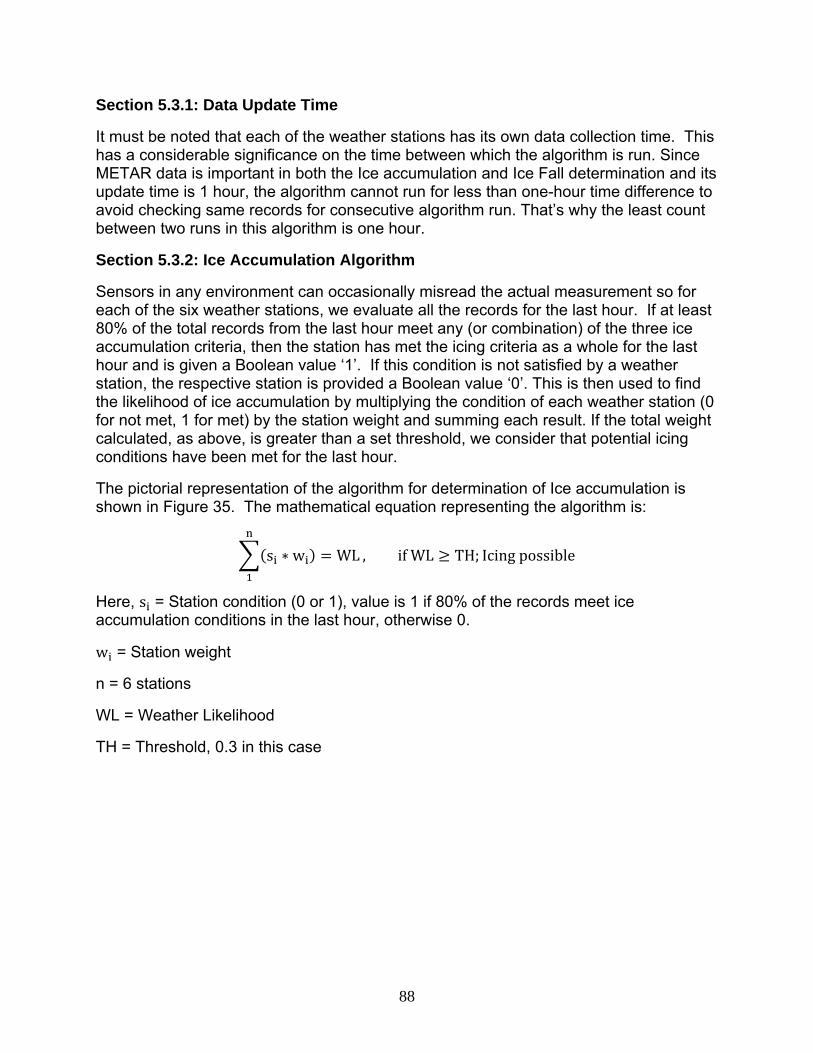
88

Section 5.3.1: Data Update Time

It must be noted that each of the weather stations has its own data collection time. This has a considerable significance on the time between which the algorithm is run. Since METAR data is important in both the Ice accumulation and Ice Fall determination and its update time is 1 hour, the algorithm cannot run for less than one-hour time difference to avoid checking same records for consecutive algorithm run. That’s why the least count between two runs in this algorithm is one hour.

Section 5.3.2: Ice Accumulation Algorithm

Sensors in any environment can occasionally misread the actual measurement so for each of the six weather stations, we evaluate all the records for the last hour. If at least 80% of the total records from the last hour meet any (or combination) of the three ice accumulation criteria, then the station has met the icing criteria as a whole for the last hour and is given a Boolean value ‘1’. If this condition is not satisfied by a weather station, the respective station is provided a Boolean value ‘0’. This is then used to find the likelihood of ice accumulation by multiplying the condition of each weather station (0 for not met, 1 for met) by the station weight and summing each result. If the total weight calculated, as above, is greater than a set threshold, we consider that potential icing conditions have been met for the last hour.

The pictorial representation of the algorithm for determination of Ice accumulation is shown in Figure 35. The mathematical equation representing the algorithm is:

s ∗ w WL , ifWL TH; Icingpossible

Here, s = Station condition (0 or 1), value is 1 if 80% of the records meet ice accumulation conditions in the last hour, otherwise 0.

w = Station weight

n = 6 stations

WL = Weather Likelihood

TH = Threshold, 0.3 in this case

Section

As seenplays a v

n 5.3.3: Sta

n in the algovery crucia

Weat

140-I

141-I

142-I

150-I

Toled

Metc

Thre

Fig

ation Indiv

orithm, w isl role in det

Tab

ther Station

R 475 @ US

R 75 @ SLM

-280 @ VGC

-280 @ Libb

do Express A

alf Field Airp

shold weig

ure 35: Ice D

idual Weig

s the weightermining th

le 22: Wea

n

S 23 Split

M 4.9 475 S

CS

bey Road

Airport

port

ht: 0.3

89

Determination

ghts

t/vote provihe ice accre

ather Statio

Statio

RWIS

plit RWIS

RWIS

RWIS

Airpor

Airpor

n Algorithm

ided to eacetion or ice

on Weights

on Type W

0

0

0

0

rt 0

rt 0

ch weather shedding l

s

Weight

0.1

0.1

0.3

0.1

0.3

0.3

station. Thiikelihood.

is

90

These station weights are based on two factors listed below:

(1) Station’s geographic location relative to the VGCS Bridge – Since the ice conditions at VGCS Bridge is to be determined; it is obvious to provide stations near to VGCS high weights. As seen in the Figure 34, the weather stations distances from the VGCS Bridge influences weight, so the weather station on the bridge has the highest weight.

(2) Amount of useful weather information that could be retrieved – As it can be seen in section 5.2.3, the weather data from METAR measurements offers more precipitation type parameters for ice accumulation determination and all the three ice accumulation criterions can be determined by METAR measurements, airports are given high weights in spite of their larger distance from VGCS Bridge.

Section 5.3.4: Threshold weights

Once the hourly weather data are utilized to determine whether ice accretion criterions is/are met for individual weather stations, the results from each station can be used to determine ice accretion as a whole. In this algorithm, [0.3] has been taken as the threshold weight. In future if we want to disregard one of the stations, we just need to make its weight zero without having any change in the algorithm. If we want to add a new weather station, we just need to add one more element in the weight array, which will suffice our need.

Here, we want to briefly discuss the origin of the somewhat arbitrary selection of the voting weight and matching threshold of 0.3 in the dashboard algorithm. This decision goes back to the very start of the dashboard and work done at UC on the initial dashboard. At the time, we anticipated using multiple weather sources as voters each with individual weights all voting together. An alert would be set if the total votes exceeded a predetermined threshold. This is the basic scheme we use today. At the time, we did not know how many voters would be included or what the threshold would be set to. We adopted a "metric" system of sorts giving voters weights which were multiples of 0.1 figuring this would give us enough latitude to make adjustments. As time went on, it turned out we never had more than 3 voters for any given rule. In some rules we only had 1 voter. Thus, the weights ended up at 0.1, 0.2, or 0.3 depending on the reliability and proximity of each voter, and the threshold ended up at 0.3.

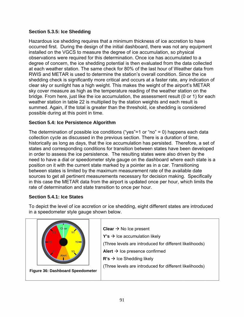
Section

Hazardooccurredinstalledobservadegree oat each RWIS ansheddinclear skysky covebridge. Fweathersummedpossible

Section

The detecollectiohistoricastates ain order need to position betweensources in this carate of d

Section

To depicin a spe

Figure 36

n 5.3.5: Ice

ous ice shed first. Durid on the VGtions were of concern,weather stand METARg check is sy or sunligher measureFrom here, r station in td. Again, if e during at t

n 5.4: Ice Pe

ermination on cycle as ally as long nd correspoto assess thave a dialon it with t

n states is lito get all p

ase the MEdeterminatio

n 5.4.1: Ice

ct the level edometer s

6: Dashboard

Shedding

dding requing the des

GCS to mearequired fo the ice sheation. The s

R is used to significantlyht has a hige as high as

just like thetable 22 is mthe total is this point in

ersistence

of possiblediscussed as days, thonding conthe ice persl or speedohe current simited by th

pertinent meETAR data fon and state

States

of ice accrestyle gauge

d Speedome

ires that a msign of the inasure the deor this deteredding potesame checkdetermine

y more criticgh weight. Ts the tempee ice accummultiplied bgreater tha

n time.

e Algorithm

ice conditiin the previ

hat the ice aditions for tsistence. Tometer stylestate markehe maximumeasuremenfrom the aire transition

etion or ice shown bel

eter

Clear

Y’s

(Three

Alert

R’s

(Three

91

minimum thnitial dashbegree of icermination. Oential is thek for 80% othe station’cal and occ

This makes erature readmulation, thby the statioan the thres

m

ons (“yes”=ious sectionaccumulatiotransition b

The resultinge gauge on ed by a poim measurets necessarport is upd to once pe

shedding, ow.

No Ice p

Ice accumu

e levels are

Ice prese

Ice Sheddi

e levels are

hickness of board, theree accumulaOnce ice haen evaluatedof the last h’s overall cocurs at a fasthe weight

ding of the we assessm

on weights shold, ice sh

=1 or “no” =n. There is on has persetween stag states wethe dashbonter as in a

ement rate ory for decis

dated once er hour.

eight differ

present

ulation likely

introduced f

ence confirm

ing likely

introduced f

ice accretie was not aation, so phyas accumuld from the d

hour of Weaondition. Sister rate, at of the airpweather sta

ment result (and each rhedding is c

= 0) happena duration

sisted. Theates have bere also drivoard wherea car. Transof the availasion makingper hour, w

rent states a

y

for different

med

for different

on to have any equipmeysical ated to a data collect

ather data fince the iceny indicatio

port’s METAation on the(0 or 1) for eresult is considered

ns each datof time,

erefore, a seeen develoven by the

e each statesitioning able date g. Specificawhich limits

are introduc

likelihoods)

likelihoods)

ent

ted rom

e on of AR e each

ta

et of oped

e is a

ally the

ced

92

Table 23 provides an explanation of the eight states.

Section 5.4.2: Ice Accumulation Persistence Algorithm

An algorithm is designed to monitor icing on the stays, which uses five different states during ice accumulation process. They are: ‘Clear’, ‘Y1’, ‘Y2’, ‘Y3’, and ‘A’.

Figure 37 shows the flow chart of the persistence algorithm for ice accumulation.

Table 23: Dial States Explanation

Nomenclature Color Significance

Clear Green No ice present on stays

Y1 Yellow Ice accretion possible. Icing conditions met for at least 1 hour, monitoring continuing

Y2 Yellow Ice accretion likely. Icing conditions met for past 8 hours, monitoring continuing.

Y3 Yellow Ice accretion very likely. Icing conditions met for past 10 hours, visual verification required.

Alert Orange Ice presence on the stays confirmed

R1 Red Ice shedding possible. Ice shedding conditions met for past 1 hour, monitoring continuing

R2 Red Ice shedding likely. Ice shedding conditions met for past 2 hours, monitoring continuing.

R3 Red Ice shedding very likely. Ice shedding conditions met for past 3 hours, visual verification required.

The pictprovided

Section

At start, ODOT rThese tw‘Y1’ signone hou

torial represd in the use

n 5.4.2.1: Tr

the state iseports preswo actions nifies icing iur or less. T

Fig

sentation ofer manual.

ransitions

s at ‘C’, cleasence of iceare done pis possible

The state tra

ure 37: Ice A

f each state

from state

ar (no ice). e) or Y1 (if tpriority wise

but the timeansition dia

93

Accumulation

e transition

e ‘Clear’

From ‘C’, tthe icing cr, the prioritye for whichgram is sho

n Flowchart

in the ice a

the states miteria are say of ‘A’ bein ice accumown in the

accumulatio

may go eithatisfied for ng higher th

mulation criteFigure 36 a

on process

er to ‘A’ (if the last houhan that of eria are meabove.

is

ur). ‘Y1’.

et is

Section

From ‘Yicing critabove tw

Section

From ‘Yicing critconditionicing is vpresenc

Once Y3

N S W O

icA samplabout th

Also at susers.

n 5.4.2.2: Tr

Y1’, the statteria are sawo conditio

n 5.4.2.3: Tr

2’, the stateteria are sans are satisvery likely tce of ice.

3 state has

No further trSend mail aWill keep seOfficials are cing conditiole mail/text

he ice accre

state Y3, da

ransitions

tes may goatisfied for ns are satis

ransitions

es may go eatisfied for asfied and alo happen a

been reach

ransition unnd text mes

ending alertneeded to

on at the brmessage is

etion on the

Figure 38

ashboard w

from state

o either to ‘Aa minimum

sfied). ‘Y2’

from state

either to ‘A’at least 8 oflso icing criand now a v

hed, the alg

ntil ODOT ressage to icis (mails/texsign onto t

ridge. s pasted be

e stays.

8: Sample Ice

will display b

94

e ‘Yellow 1

A’ (if ODOTm of 6 out osignifies ici

e ‘Yellow 2

’ (if ODOT f last 10 houteria did novisual chec

gorithm will

esponse is ing officialsxt) to officiathe dashboa

elow, which

e Accumulati

blinking Yel

’

T reports pof last 8 hoing is likely

’

reports preurs) or ‘Y1’ot satisfy fok must be d

take the fo

received. s. als until a reard and pro

h is used to

ion Message

llow signal

presence ofours) or ‘C’to happen

esence of ic (if none of r Y2 state).done to con

ollowing act

esponse is ovide respo

notifying th

e Alert

to catch the

f ice), Y2 (i’ (if none o.

ce) or ‘Y3’ (f the above . ‘Y3’ meannfirm the

tions:

received. onse on act

he icing offi

e attention

if the of the

if two

ns

tual

icials

of

After theThis led

Section

Differentshows th

At Y3, fu‘there is confirmeto ‘Y1’.

e Y3 state isthe algorith

n 5.4.3: Ice

t states usehe flow cha

urther stateice presen

ed. If the re

Figure 39

s reached, hm to move

Presence

ed in the Iceart of the alg

F

s are deternt on the stasponse say

9: Dashboard

the algorithe to the nex

Confirmat

e presencegorithm exp

Figure 40: Ice

rmined usinays’, the stays ‘there is

95

d with Ice Ac

hm will waitxt stage of t

ion

e process arplained abo

e Presence F

ng the receiate will movno ice pres

ccumulation

t for a respothe icing ev

re ‘C’, ‘Y1’,ove.

Flowchart

ved responve to ‘A’, whsent on the

Alert

onse for icevent proces

and ‘A’. Fi

nse. If the rehich meansstays’, the

e presence.ss.

gure 40 be

esponse sas ice is

state will m

.

low

ays

move

96

There are two reasons why upon receiving a negative response, the state will move to Y1 and not C.

Ice may be present on the stays but it might not be enough to cause an ice fall hazard. In that case, the response received may be negative but a more insightful move is to assign Y1 as the new state in action to the response.

In case of a mistake in submitting the response, assigning Y1 will take lesser time than ‘C’ to go to Y3 state, which is desirable.

From here, we move to the last stage of the ice events, i.e. state transition algorithm for the Ice Fall process.

Section 5.4.4: Ice Shedding Persistence Algorithm

Different states used in the Ice Fall process are ‘R1’, ‘R2’, ‘R3’, ‘A’, and ‘C’. Figure 41 below shows the flow chart of the algorithm explained above.

The pictprovided

Section

From ‘Astays) odone pripossibleaccumuTherefor

torial represd in the use

n 5.4.4.1: Tr

’, the statesr ‘R1’ (if theiority wise,

e. Since thelation procere, if the ice

F

sentation ofer manual.

ransitions

s may go ee ice fall crithe priority

e ice sheddiess, an alere fall criteria

Figure 41: Ice

f each state

from state

ither to ‘C’ teria are saof ‘C’ being

ing processrting systema are met d

97

e Shedding F

e transition

e ‘Alert’

(if ODOT reatisfied for tg higher thas is faster am is implemduring the la

Flowchart

in the ice s

eports that the last houan that of ‘R

and more crmented at evast hour, th

shedding pr

there is no ur). These tR1’. ‘R1’ meritical than tvery state ce state will

rocess is

ice on the two actions eans ice fathe ice change. be change

are ll is

ed

from A tnotifying

Section

From ‘R(ice sheconditionis sent to

Section

From ‘R(ice sheconditionmessag

Once R3

N S W O

icA samplabout th

Also at susers as

After thereceivedreceivedtransitiosolar radnight. A

o R1, and ag about the

n 5.4.4.2: Tr

R1’, the statedding criterns are satiso icing offic

n 5.4.4.3: Tr

R2’, the statedding criterns are satise is sent to

3 state has

No further trSend mail aWill keep seOfficials are cing conditiole mail/text

he ice accre

state R3, das shown in

e R3 state id is “no ice d is “ice pren for R3 to diation dimi

A possible s

also e-mailsweather an

ransitions

es may go ria are satissfied). ‘R2’ cials notifyin

ransitions

es may go ria are satissfied). ‘R3’ icing officia

been reac

ransition unnd text mes

ending alertneeded to

on at the brmessage is

etion on the

ashboard wFigure 43.

s reached, present on

esent on the‘A” would b

inishes. Thscenario cau

Figure 4

s and text mnd the state

from state

either to ‘Csfied for themeans ice ng them ab

from state

either to ‘Csfied for themeans ice als notifying

hed, the alg

ntil ODOT ressage to icis (mails/texsign onto t

ridge. s pasted be

e stays.

will display b

the algoriththe stays”,

e stays”, thebe caused bhis would musing the tr

42: Sample I

98

messages aes.

e ‘Red 1’

C’ (if ODOT e last hour) fall is likelyout the cha

e ‘Red 2’

C’ (if ODOT e last hour) shedding isg them abo

gorithm will

esponse is ing officialsxt) to officiathe dashboa

elow, which

blinking Re

hm will wait, the state we state will by nightfall

make it likelyransition to

Ice Shedding

are sent to

reports no or ‘A’ (if no

y to happenange.

reports no or ‘R1’ (no

s very likelyout the chan

l take the fo

received. s. als until a reard and pro

h is used to

d signal to

t for a respowill change change to when the t

y the ice woC would be

g Message A

the ODOT

presence oone of the a. Also mail/

presence one of the ay to happennge.

ollowing act

esponse is ovide respo

notifying th

catch the a

onse. If theto ‘C’ and ‘A’. For extemperatureould persiste ice fall.

Alert

officials

of ice) or ‘Rabove two /text messa

of ice) or ‘Rbove two

n. Also mail

tions:

received. onse on act

he icing offi

attention of

e response if the respoample, a e drops andt through th

R2’

age

R3’

l/text

tual

icials

onse

d the he

The procbe seen

Section

The algohow the algorithmof the aldata fromautomat

cess flow fo in the proc

n 5.5: Mon

orithm desigalgorithm i

m results argorithm anm and mante the collec

Figure

or ice accumcess state d

itor Websi

gn and woris implemenre made acd the dashb

nage connection and d

Figure 44: S

43: Dashboa

mulation, icdiagram sho

te

rking is expnted for theccessible toboard was ctivity betwata wareho

State Transiti

99

ard with Ice

ce presenceown in Figu

plained in abe front end uo users is thdivided into

ween separaousing of we

ions possibl

Shedding Al

e and ice faure 44 below

bove Sectiouser. The to

he ‘Dashboao three partate systemseather mea

e from Red L

lert

all combinew.

ons. This Sool throughard’. The imts in order ts. The first asurements

Email & Text Msg

Level 3

d together

ection explh which the mplementatto integratepart was to

s of the RW

can

ains

tion e o

WIS

100

stations and airport METAR data. These processes needed to be stable and robust so we had a reliable set of weather measurements from all the necessary sources. This system was not required for development of the next part, but having the necessary data stored locally inherently increases performance, reliability and robustness. From the developed algorithm and all the necessary conditions, software was developed to carry out the automated evaluation process and scheduled to run once per hour as previously mentioned. Finally a set of web pages were developed which is called the dashboard.

As defined above the data collection and the results of the algorithm is stored in the database running in UCII server. This information is made available to the user through dashboard. Below listed are few of the dashboard’s important features:

Provide user-friendly speedo-style display of current icing status Collect and maintain database of weather conditions Automatically process incoming weather data and update icing status Generate alerts during icing events User-friendly display and navigation of weather data User-friendly display and navigation of icing event history

Section 5.5.1: Dashboard Main Panel

The main panel of the dashboard contains the icing speedometer showing all the states including {G, Y1, Y2, Y3, O, R1, R2, and R3}. The main panel also includes the reporting function for ODOT, which can be used to report icing status after visual inspection. The ticker on the main panel shows icing conditions of the last 48 hours. The main panel includes the links to all other pages of the dashboard.

In Figure 45, a screen shot of the web site is illustrated showing the dashboard main panel. As shown, the dashboard main panel provides a user-friendly dial that shows the icing status. The dashboard main panel is changed when icing reaches the level when an alert is necessary (e.g., see Figures 39 and 43).

Section

Dashboareadingsare alsothis purpprovidedtransporbe useddashboamonitorevarious Basically

L S W S

This secthe accoGoogle

There ar(Toledo being m

n 5.5.2: Wea

ard includes are shown cameras inpose Googld by Googlertation. It ha to develop

ard is used ed for detersites, their y the featur

ocating weShowing theWeather reaSite informaction is a waordion labelmap will op

re two greeExpress Aionitored by

F

ather Map

s an interacn and whernstalled on le Maps APe, which offas an extenp custom Go

as an interrmining the past/currenres included

ather statioe live cameradings for ation of all thalkthrough led “Map (Wpen which h

en markers irport) and y the dashb

Figure 45: Da

ctive map ore historicalthe bridge

PI is used. Gfers street lndable API oogle Mapsrface to proicing cond

nt weather cd in the wea

ons ra installed

all stationshe stationsof the work

Weather Dahas several

written ‘A’ oKTDZ (Met

board.

101

ashboard Ma

of the weath readings cthat can be

Google Mapevel maps (Applications based apvide the deitions at VGconditions aather map a

on the site

king of the Gata by Loca

markers o

on it. Thesetcalf Field A

ain Panel

her stationscan be plotte seen fromps is a freefor pedestrn Programmplications. T

etails about GCS. It alsoalong with aare:

e

Google mation)” on thn it (e.g., se

e are the twAirport) who

s where curted on a tim

m this intera web mapprians, cars, ming InterfaThe Googlethe various

o contains ta few refere

p on the dahe dashboaee Figure 3

wo Airports ose weathe

rrent sensomeline. Theactive map.ping service

and publicace) that cae map on ths sites beinthe locationence links.

ashboard. Ord is clicked

34).

namely KTer data are

or re For

e an he

ng n of

Once d, a

TOL

102

There are four red markers written ‘R’ on it. These are the four RWIS stations namely Site 140-IR 475 @ US 23 Split, Site 141-IR 75 @ SLM 4.9 475 Split, Site 142-I-280 @ Veterans Glass City Skyway, and Site 150-I-280 @ Libbey Rd whose weather data are being monitored by the dashboard.

There are three yellow markers written ‘L’ on it. These are the local weather stations near to the VGCS Bridge. They are: East Toledo, Oregon. These are not considered in the algorithm.

The pink marker is the link to the live cameras installed on VGCS.

RWIS Stations

Red markers on the map represent RWIS stations. On clicking, an information box will be popped up that contains the weather station information, station id, current weather conditions and last 48 hours graphs to atmospheric and surface weather readings.

Clicking the “Buckeye Traffic Readings” link on the information window opens up a new window having the weather reading from http://www.buckeyetraffic.org/.

Clicking all other links on the information window opens up a new window having the last 48 hours weather readings. Below is an example for last 48 hours plot for the parameter ‘Air Temperature’. The ‘Export’ button will export the Air Temperature data for the last 48 hours into the excel sheet.

Airports

Green markers on the map represent nearby airports. On clicking them, an information box will be popped up that contains the current METAR report, plots of last 24 hours METAR reports, last 4 hours PIREP readings, plots of PIREP Icing information since Nov 13 2010, and WIKI references to METAR & PIREP.

Clicking the “METAR” link on the information window opens up a new window having the current METAR reading from: http://english.wunderground.com/history/airport/

Clicking the “PIREP” link on the information window opens up a new window having the latest PIREP readings from: http://aviationweather.gov/adds/pireps/

Local Weather Stations

Yellow markers on the map represent nearby weather stations. On clicking them, an information box will be popped up that contains the weather information at the local station. Attached below is the screenshot for the local weather station: East Toledo.

Clicking the “Rapid Fire Panel” link opens up a new window having the weather information from: http://www.wunderground.com/weatherstation

Clicking the “More information” link opens up a new window having the weather information from: http://www.wunderground.com/weatherstation

Live Ca

Pink maSkyway every fiv

Section

The Histfor the uexplanatthe dash

The mai

(a) List o

User canthe Figuupdate bany eve

(b) List odashboathe pers

(c) Sumweatherproduce

mera

arkers on thBridge. Cli

ve seconds

n 5.5.3: His

tory sectionusers for antion of the shboard.

in functiona

of events (s

n select twoure above, tbutton will dnt will provi

of responseard over theson who pos

mmary: Thisr stations. Ued and whic

e map reprcking on an.

tory

n of the Dasnalyzing andsame. Figu

Fi

alities of this

states other

o dates bettwo dates adisplay all tide the cau

es receivede time are dsted the co

s section prUser can sech is then sh

resent link tny will get t

shboard prod reporting re 46 below

igure 46: Das

s section of

r than green

tween whicare selectedhe events ose of the ev

by dashbodisplayed inomment. Giv

ovides statelect two dahowed up u

103

to the four lhe live view

ovides manpurposes.

w shows the

shboard Hist

f the dashb

n) between

h the statesd i.e. 03/11/occurred bevent.

oard: All then this sectioven below i

istics of theates betweeupon clickin

live cameraw with the im

ny additionaThis sectioe main pan

tory Panel

board includ

n dates sele

s need to b/2011 and 0etween thes

e responseson. This alsis a screen

e weather pen which theng the upda

as installed mages gett

al features ton provides nel of the hi

de:

ected by the

be displayed05/28/2011se dates. A

s received bo includes shot.

parameters e statistics

ate button.

at the Veteting refresh

that are usea detailed story sectio

e user:

d. As show, and a clic

Also clicking

by the the name o

for all the sneeds to b

eran ed

eful

on of

n in ck on g on

of

six be

104

Section 5.5.4: Implementation Tools

To implement and design dashboard functionalities, several languages/tools/software are used. The list for the same is provided below:

Table 24: Tools Used To Design Dashboard

Category Tool Used Purpose

Programming Language Python Data Pulling

Main Algorithm

Scripting Language PHP Website design

Database MySQL Data Storage

Graphing Tools JPGraph

Matplotlib

Weather charts

Test results

Map Google Maps API Weather Map

Visuals Microsoft Visio, JavaScript Flowchart

Section 5.6: Performance Testing

The dashboard became fully functional in the month of January 2011 (Jan 15 2011, 18:05:05) and since then it has been running on the University of Cincinnati Infrastructure Institute server, monitoring the weather conditions at Veterans’ Glass City Skyway. To test the performance of the dashboard, rigorous testing methods were implemented, which is the main agenda in this Section. The various tests done on the dashboard can be divided into two main sections:

1. System reliability test a. Weather station dependability

2. Ground truth a. Study of Feb 2011 ice events b. Study of past ice events

Section 5.6.1: System Reliability Test

Checking the weather data obtained from various RWIS stations constitutes the reliability test. For this purpose, all RWIS stations within 10 miles radius of the VGCS site are considered for the study. This could also be used as a cross check for the choice of weather stations and provides us a better insight on whether the stations needs to be changed/added for future ice analysis. A complete list of RWIS and Airports stations used for the study is given in the table below: Section 5.6.1.1: Weather stations dependability

Weather readings are checked for the above-mentioned stations during the period when ice events occurred from 2006 through 2009. A table is provided for the date/time for which weather readings are studied.

105

Table 25: Dates for Past Ice Events that were Tested

Icing Events during last 3 years Dates for which the data is studied

12 Dec 2007 2 Dec 2007 3:00PM - 23 Dec 2007 3:00PM

28 Mar 2008 18 Mar 2008 3:00PM – 8 Apr 2008 3:00PM

17 Dec 2008 7 Dec 2008 3:00PM – 28 Dec 2008 3:00PM

3 Mar 2009 24 Dec 2008 3:00PM – 14 Jan 2009 3:00PM

The following parameters are checked for stations fidelity:

Null readings: Number of readings which doesn’t have any value Bad readings: Checked +/- 3 standard deviation for outliers

These checks are done for all the four icing events and the results are tabulated below:

Table 26:Weather Statistics for December 12, 2007 Ice Event

Dec 12 2007

Site 137

Site 139

Site 140

Site 141

Site 142

Site 146

Site 147

Site 150

Airport KTOL

Airport KTDZ

Total number of records 5777 5892 5264 5834 5778 5566 5911 5868 841 828

Temperature (deg F)

Max Temperature

54 54 54 54 54 54 54 54 53.6 54

Min Temperature

6 10 11 14 13 7 8 6 8.1 8.1

Null count 0 0 1 0 0 0 11 0 0 0

Precipitation (Occurences)

'None' 4761 4817 4396 4621 4871 4270 4769 4771 0 0

'Yes' 1010 1073 0 1206 0 0 1012 1073 0 0

'Rain' 0 0 422 0 322 444 0 0 108 143

'Snow' 0 0 377 0 361 422 0 0 107 84

'Fog' 0 0 0 0 0 0 0 0 18 13

Null count 6 2 69 7 224 430 130 24 608 588

RWIS sites 140, 141, 142, 150 are used in the algorithm and it can be seen from the table that the precipitation types reading from sites 141 and 150 do not read anything except ‘Yes’ and ‘None’. Whereas the RWIS sites 146 shows a good dependability in terms of weather readings.

A similar analysis was done for the other icing events. All this analysis leads to the following conclusions:

RWIS sites 137, 139, 141, 147, 150 – have just “Yes” or “None” as types of precipitation, so they cannot be used for ice determination

106

RWIS sites 141, 146, 150 categorizes all the precipitation types so they can be used for ice determination

Null or bad readings for all the RWIS sites are 82 out of 182,222 records in total i.e. 0.045%, which is a very small number and thus sites 141, 146 and 150 can be used in the ice determination algorithm without having too many outliers

Section 5.6.2: Ground Truth

After the tests performed on data reliability, the next phase is the testing of the actual algorithm. Since the inception of dashboard on Jan 15, 2011, there have been several occurrences of icing precipitation on the VGCS site.

Section 5.6.2.1: Study of Feb 2011 ice events

Ice Accretion detected by the Dashboard

Table below provides a statistics on the algorithm results within the period between January 15 and June 15, 2011.

Table 27: Summary of Events when Ice Accumulation occurred in 2011

Ice Events Dates

Maximum Level

reached Reason Comments

Feb 02 2011 Y1 Freezing

Rain No action taken since ice accretion was minimal





Feb 20-25 2011

G-Y3-O-R3

Multiple Described in detail

Feb 25-27 2011

Y3 Freezing

Rain

Due to bad precipitation data from VGCS RWIS station, the dial was stuck at Y3. So, it was manually reset

Mar 5-6 2011

Y2 Wet

Snow Ice accretion occurred but it was not enough to cause Ice fall hazard. No action taken

Mar 10-11 2011

Y2 Wet

Snow Ice accretion occurred but it was not enough to cause Ice fall hazard. No action taken

Mar 30 2011 Y1 Wet

Snow No action taken since ice accretion was minimal

Apr 18 2011 Y1 Wet

Snow No action taken since ice accretion was minimal

As it canseveral only one

The eve

Feb 20: VGCS mthe critethe two 21:00. T22:00, thwaiting f

Local TVtemperathe forecwas scatempera

Figure 4

n be seen toccurrence

e event had

ent from Feb

The ice acmet freezingria for freezairports and

The ice accuhus the dialfor the ice s

V forecast: ature. On a casters pre

attered rain atures and p

48 shows th

hat in the pes when thed sufficient i

b 20-25 is d

ccretion prog rain criterzing rain cod the RWISumulation wl in the dasshedding co

The forecalocal televidicted snowor freezingprecipitation

Figure

he close up

period from e ice accretice to pose

described in

ocess starteia and the d

onstantly meS at VGCS.was confirmhboard moonditions to

ast for that nsion stationw changing rain with an, the cond

47: Weather

view of ice

107

Jan 15 to Jion was deice sheddi

n detail bel

ed at 15:00 dial in the det for 8 hou This cause

med by the vved to Oran

o come.

night was frn’s weatherg to freezingadditional icitions were

r Summary o

e accretion o

June 15 20tected by thng hazard.

low:

because thdashboard urs in one oed the dashvisual inspenge, i.e. ale

reezing rainr website (Sg rain. The ce accumulae conducive

on Feb 20, 20

on Feb 20,

11, there hhe dashboa

he RWIS stbecame Y1

or more stathboard to dection doneert. Now the

n, then a drStorm Trackupdate for ation. With

e to ice accu

011

2011.

ave been ard out of w

ation at the1. After thentions includisplay Y3 a

e by UT at e algorithm

rop in ker 11, 201the overniglow

umulation.

which

e n, ding at

m is

1), ght

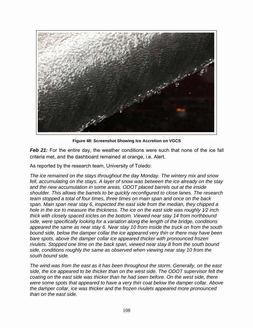
Feb 21:criteria m

As repor

The ice fell, accuand the shouldeteam stospan. Mhole in tthick witside, weappearebound sbare sporivulets. side, consouth bo

The winside, thecoating were sothe damthan on

: For the enmet, and th

rted by the

remained oumulating onew accumr. This allowopped a tot

Main span nethe ice to mth closely spere specificaed the sameside, below ots, above tStopped o

nditions rouound side.

d was frome ice appeaon the eastme spots th

mper collar, the east sid

Figure 48: S

ntire day, te dashboar

research te

on the stayson the staysmulation in sws the barrtal of four timear stay 6,

measure thepaced icicleally lookinge as near stthe dampethe damperne time on ughly the sa

m the east aared to be tht side was that appeareice was thicde.

Screenshot S

he weatherd remained

eam, Unive

s throughous. A layer osome areasrels to be qumes, three inspected t

e thickness.es on the b

g for a variatay 6. Nearr collar the r collar ice athe back sp

ame as obs

s it has beehicker than thicker thaned to have cker and th

108

Showing Ice

r conditionsd at orange

ersity of Tole

ut the day Mof snow wass. ODOT pluickly recontimes on mthe east sidThe ice on

ottom. Viewtion along tr stay 10 froice appearappeared thpan, vieweserved whe

en throughoon the wes

n he had sea very thin

he frozen riv

Accretion on

s were suce, i.e. Alert.

edo:

Monday. Ths between tlaced barrenfigured to

main span ade from the n the east swed near stthe length oom inside thred very thinthicker with d near stay

en viewing n

out the storst side. Theeen before.

coat belowvulets appe

n VGCS

ch that non

he wintery mthe ice alreels out at thclose lanes

and once onmedian, th

side was routay 14 fromof the bridghe truck on in or there mpronounce

y 8 from thenear stay 1

rm. Generae ODOT supOn the we

w the dampeeared more

e of the ice

mix and snoady on the e inside s. The resen the back hey chippedughly 1⁄2 in

m northbounge, condition

from the somay have bed frozen e south bou0 from the

ally, on the epervisor felst side, theer collar. Abpronounce

e fall

ow stay

earch

d a nch nd ns outh

been

und

east lt the

ere bove ed

Both theit could bfurther u

Feb 22:criteria m

e east and tbe seen. Hup than abo

: For the enmet, and th

the west sidHowever, it iout mid-heig

Figure

ntire day, te dashboar

des, the iceis impossiblght.

49: Weather

he weatherd remained

109

e above thele to discer

r Summary o

r conditionsd at orange

e collar appern anything

on Feb 21, 20

s were suce, i.e. Alert.

eared unifomore than

011

ch that non

orm as highgross icing

e of the ice

h as g

e fall

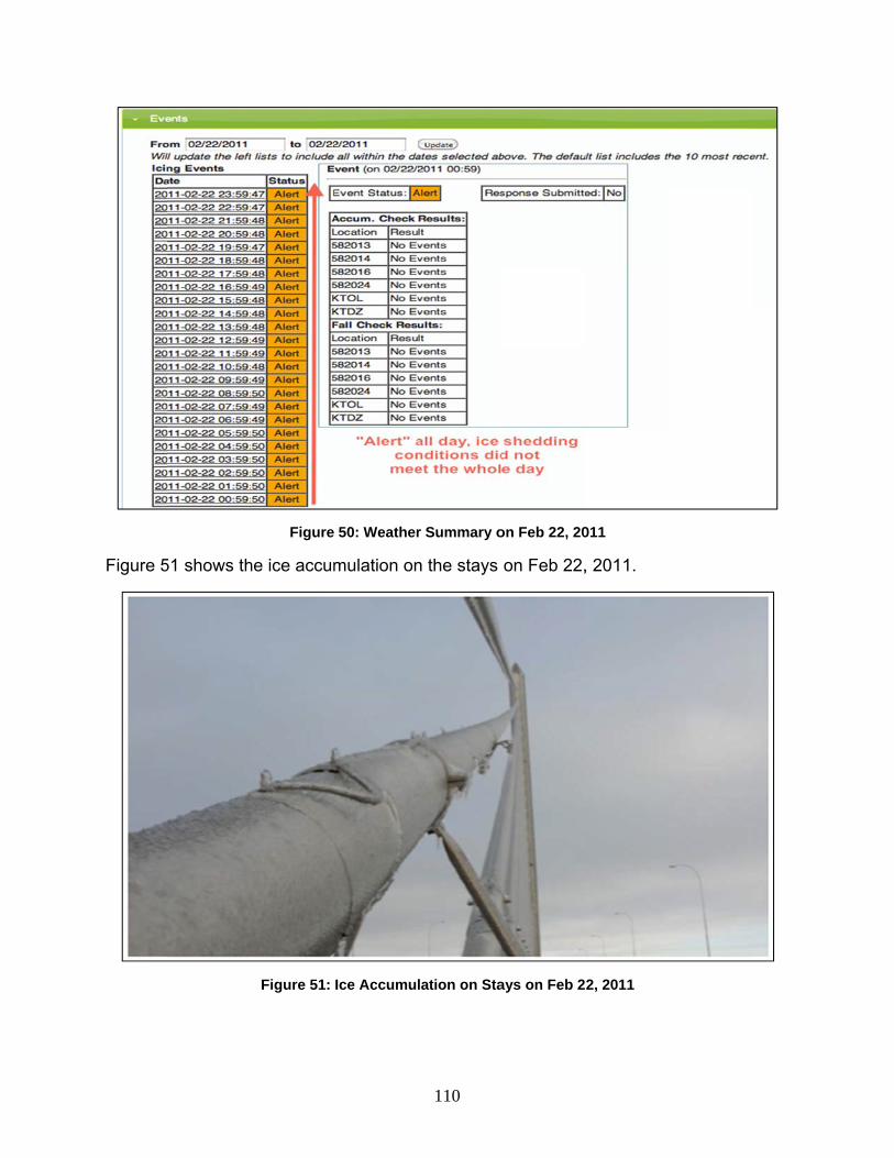
Figure 5

51 shows th

Figure

he ice accum

Figure 51:

50: Weather

mulation on

Ice Accumul

110

r Summary o

n the stays

lation on Sta

on Feb 22, 20

on Feb 22,

ays on Feb 2

011

, 2011.

2, 2011

111

Feb 23: For the entire day, the weather conditions were such that none of the ice fall criteria met, and the dashboard remained at orange, i.e. Alert. But there is one thing that caught the attention. The research team from The University of Toledo measured the temperature between stay and ice with a K contact thermocouple. One noticing observation was that temperature between the ice and stays (interstice) and atmospheric temperature were different. It was observed that interstice temperature was greater than air temperature. At 1:00PM interstice temperature was recorded 32°F whereas air temperature was 27°F. This may be due to greenhouse effect occurring in between ice and stays. Below provided are the results from The University of Toledo.

Table 28: Interstice Temperature on February 23, 2011

Time Interstice

Temperature Stay Note

8:15 AM 24 °F 20B No visible liquid water 8:50 AM 24 °F N/A No visible liquid water 9:20 AM 24 °F 20B 9:30 AM 28 °F 15B 9:45 AM 26 °F 11B Liquid water under ice

12:15 PM 30 °F 19B Liquid water under ice. Large pieces 1:00 PM 31 °F 20B 1:00 PM 32 °F 19B 1:15 PM 35 °F 18B Liquid water under ice. Sheets break 2:55 PM 32 °F 20B Liquid water that had bled from 3:57 PM 32 °F 20B 5:23 PM 31 °F 19B Liquid water under ice. Sheets break

Feb 24: At 7:00 am, the Airport at Metcalf field reported temperature above 32F, thus for the first time the dashboard showed R1 to indicate possible ice shedding. It continued for two more hours and the dashboard moved to R3 at 9:00 am. The entire contribution goes to Metcalf Field Airport. Dashboard then generated alert signals and requested visual inspection. At 16:00, dashboard received a response from UT that little ice is still remaining, so the dashboard moved to orange. The comment for the same, taken from the dashboard, is pasted below:

“As per discussion with ODOT and Dr. Nims, most of the ice has shed due to rise in temperature but a little ice is still remaining on the stays.”

Again at 18:00, due to high temperature at each station, dashboard moved to R1 and in two more hours, it moved to R3. As programmed, it sent alert signals for visual inspection at 20:00. Now dashboard is at R3 and waiting for a reply.

Feb 25: Ice Accu

“Temps sheddin

With thisthat ice received

“No ice aODOT h

At 00:59 aumulation is

dropping wg.”

s, dashboarhas shed a

d at 7:59 am

apparent. Ahas reopene

Figure

Figu

m, a respos again pos

with ice pers

rd moved toand the posm is pasted

Additional aed all lanes

52: Weather

ure 53: Exam

nse was ressible. Com

sisting. Sec

o orange agsibility of sebelow:

accumulatios.”

112

r Summary o

ple of Ice Sh

eceived thatmment from

cond round

gain. Finallyecond roun

on expected

on Feb 24, 20

hedding Alert

t temperatuthe dashbo

of possible

y at 7:59 amnd of icing h

d last eveni

011

rt

ure is againoard is past

e icing follow

m, a responhas diluted.

ng did not

dropping ated below.

wed by

nse receiveThe respo

materialize

and

ed nse

.

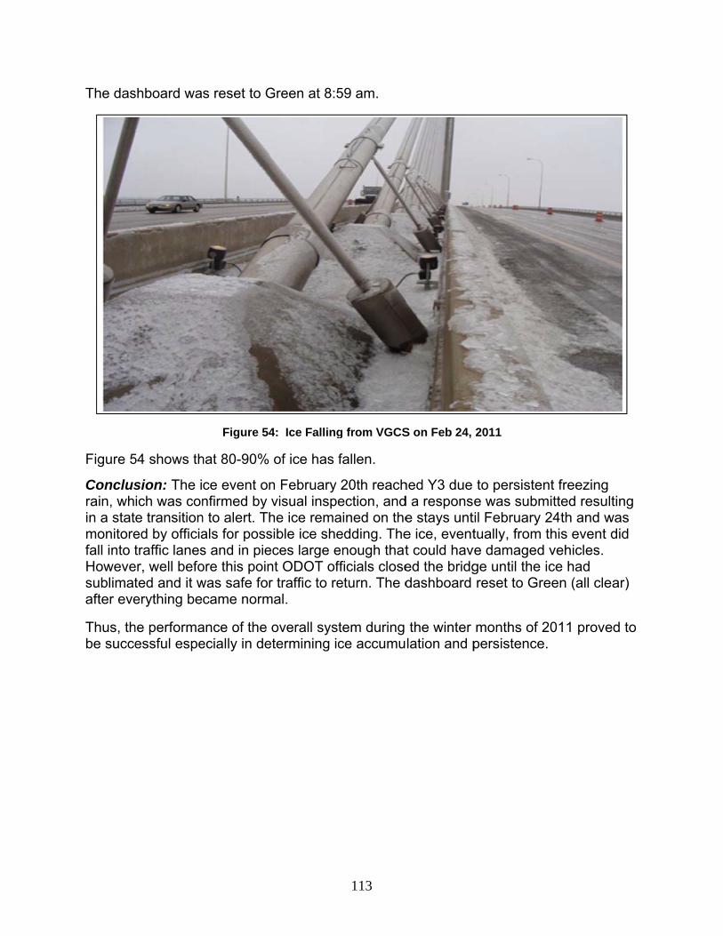
The das

Figure 5

Conclusrain, whin a statmonitorefall into tHowevesublimatafter eve

Thus, thbe succe

shboard wa

54 shows th

sion: The iich was cone transitioned by officiatraffic lanes

er, well befoted and it werything be

he performaessful espe

s reset to G

Figure 54

hat 80-90%

ce event onnfirmed by

n to alert. Thals for posss and in pieore this poinwas safe forcame norm

ance of the ecially in de

Green at 8:5

4: Ice Falling

of ice has

n February visual inspehe ice remasible ice sheeces large ent ODOT ofr traffic to re

mal.

overall sysetermining ic

113

59 am.

g from VGCS

fallen.

20th reachection, andained on theedding. Theenough thatfficials closeeturn. The d

tem during ce accumu

S on Feb 24,

hed Y3 due d a response stays unte ice, eventt could haved the bridgdashboard

the winter lation and p

2011

to persistee was submtil February tually, from

ve damagedge until the reset to Gr

months of persistence

ent freezingmitted resu24th and w this event

d vehicles. ice had

reen (all cle

2011 provee.

lting was did

ear)

ed to

The ovethe actuand the Fab 21 t

Paramet

1 Tem

2 Ave

3 Ice a

4 Ice s

Figure 52011), leThe grapas the aare showby red cmet (as when ice

erall algorithal weather algorithm rto Mar 06 2

ters shown

mperature v

rage tempe

accretion c

shedding c

56 is a two-aeft y-axis isph shows thverage temwn in blue ccrosses. The

per the alge-shedding

Figure

hm can be sdata (temp

response on2011.

in the grap

versus time

erature vers

riteria satis

riteria satis

axis graph, the tempehe tempera

mperature vcrosses whe yellow triaorithm desc criteria are

55: Weather

simulated operature andn those dat

ph:

(for six wea

sus time (ag

fied

fied

in which x-rature in F,

ature versusersus time.ereas snowangles are cribed in abe met (as pe

114

r Summary o

on a graph ad precipitatta. The sim

ather statio

ggregated f

-axis is the and right ys time grap. The rain ow occurrencthe hours w

bove Sectioer the algor

on Feb 25, 20

as shown btion types) oulation is d

on)

for six weat

time in daty-axis is theph for all theoccurrencesce (in % of when ice acons). The rerithm descr

011

below. The of the six wone for the

ther station

tes (Feb 21e % of snowe weather ss (in % of rerecord per ccumulationed squares ribed in abo

graph showweather state time period

n)

to Mar 06 w/rain per hstations as wecord per hhour) is sh

n criteria arare the ho

ove Section

ws tions d

hour. well

hour) own

re urs

ns).

Weathe

The anasection eit explainstudy is and weafactors acondition27 2011tab of th

Table 29can be s582024.requiredmain coand onlyprecipitaand shoand numrain is ththe x-ax

r Station P

alysis of algexplains thens the contdone as it

ather stationaffecting thens at all the (date of cr

he dashboa

9 shows temseen that th Hencefort

d for Ice accntribution toy few weathation type’s wn in the F

mber of houhe leading cxis and the n

Figure 56:

Performanc

orithm for oe contributiribution of aprovides a n so that in e icing and e six weathereation of thrd.

mperature ahere is no ‘Rh, these twcretion. To owards the her stations

contributioFigure 57b. urs meeting criteria out number of h

Feb 24, 2011

ce Evaluat

one icing evon of each all the six wdeeper undfuture the de-icing. T

er stations his docume

and precipiRain’ or ‘Sno stations ccomplimenice accreti

s. During theon and each

Figure 57aicing criterof the threehours meet

115

1 Algorithm P

ion

vent has beicing criter

weather statderstandingfocus could

The table beduring the

ent). This re

tation readnow’ readingcannot contt this, two fon processe entire iceh weather sa shows theria on the y-e. Figure 57ting icing cr

Performance

een done inria towards tions towarg about thed be laid onelow summperiod betw

eport is gen

ings for thegs for RWIStribute to thfigures are s is limited te event’s 68station’s cone three icing-axis. It can7b shows thriterion on t

e Graph

n the abovethose icing

rds the icing role of eac

n the most imarizes the oween Jan 1erated from

e six weatheS site 5820

he necessadrawn to shto few weat8 hours, eacntribution wg criterion on be seen thhe six weatthe y-axis. I

e section. Tg events. Alg events. Tch icing critemportant overall wea5 2011 to M

m the “Histo

er stations.014 and sitery criteria how that thther criterioch of the

was countedon the x-axihat freezingther stationsIt can be se

his so, his eria

ather May ory”

It e

e ons

d s g s on een

that out airports

WeaPara

TemAverMinimMaxPrecCleaRainSnowOthe

Figure 5

Thus it cRain had

0

10

20

30

40

50

60

Numberofhours

of the six ware the lea

T

Weather

ather ameters

KT(ToExAirME

perature (°Frage 39mum -4.imum 87

cipitation ar 14n 10w 60ers 47

57a: Contrib

Figu

can be concd the most

0

0

0

0

0

0

0

wetsnow

weather stading contrib

Table 29: S

r Report for

TOL oledo

xpress rport) ETAR

K(FAM

F) 9.0 3.0 -

7.1 8

469 109 80 47 1

bution by the

re 57 : Contr

cluded that influence o

w freezingrai

IcingConditi

tions, the Rbutor.

tation Com

r VGCS Brid

KTDZ Metcalf

Field Airport) METAR

R58(1@SLu

39.8 298.0 -4

88.0 82

1400 4081 2344 521 28

e three criter

ribution of th

the RWIS on the ice a

in freezingfog

ions

116

RWIS statio

mparison fo

dge from Ja

RWIS Site 82013 140-I-475

@ US-23 plit - ucas Co.)

9.9 4.0 2.0

041 3 21 866

ria Figure

he Icing Crite

station on tccumulatio

g

1

2

3

4

5

Numberofhours

on at the VG

or the 2011

an 15 2011 t

RWIS Site582014 (141-I-75 @ I-475Split - SLM4.9 Lucas)

40.6 -3.0 87.8

13461 XXX XXX 3509

e 57b: Contr

eria and Wea

the VGCS on decision

0

10

20

30

40

50

VGCS Station

GCS Bridge

1 Winter

to June 15 2

e

5 M

RWIS Site 582016 (142-I-280 @VGCS)

35.8 -3.0 82.0

9941 2309 1579 67

ribution by th

ather Stations

Bridge andprocess.

WeatherSta

e and the tw

2011

@

RWIS Site 582024 (150-I-280 @Libbey Road)

39.6 -19.1 84.4

6112 XXX XXX 10812

he six station

s

the Freezi

ations

wo

@

ns

ng

Section

Dashboaanalysisvisual obthe ice faccumuexamplebetweenbelow 32radiationexampleassumptmeasurevisual obstation sdashboa

Figure Weathe

Thus, it should bAlso, insice shedentire pris run, abecamethe ice g

7:04AM

Watt/m^2

n 5.6.2.2: C

ard has dons done on thbservationsfall detectiolation detec

e, it was non the ice an2F but the sn, which coe in the earltion, data wes and recobservation started to risard moved

58a: Solar Rer Station in

is proposedbe installed stallation ofdding eventroject, meat least while clear (with

got melted.

8:16

AM

SolarR

omments

ne pretty whe algorithms concludesn speed anction and imted that afte

nd the stay, stay and aiuld heat uply morning

was collecteords solar ratimeline. Tse close to to R1.

Radiation MeOregon, OH

Figure 58:

d that for beat VGCS s

f a sensor mts. In additiosures coulde detecting

h ice on stay

8:16AM

Radiatio

ell in detecm results ans that additind accuracymprove the er taking tethat the atmr gap could

p the stay wor first sigh

ed from a wadiation, w

This plot sho7:00am, w

easurementsH)

: Solar Radia

etter ice shso that it cameasuring son, since Icd be taken t ice sheddiys), ice star

9:28AM

on2/24

117

ting ice accnd Universional inform

y. This wouoverall sys

emperature mospheric

d be above well before tht of clear sweather stathich was plows that the

which is app

s (KOHORE

ation Variatio

edding detean measuresolar radiatce sheddingto decreaseng. As it warted melting

10:40AM

4/2011

cumulation ty of Toledo

mation woululd also incstem’s accu

readings otemperatur32F. This ithe air tempky coveragtion approxlotted and ce solar radi

proximately

EGO1 Figtem

on on Feb 24

ection, a th the exact t

tion could reg events aree the time bas seen thag and in les

11:52AM

T

each time, o’s responsd be neede

crease perfouracy and reon the stay re readingss most likeperature incge). Followximately 3 mcompared wiation at thithe same t

ure 58b: Memp and ice g

4, 2011

hermocoupltemperaturesult in bette faster andbetween what when thess than 2 ho

Temp Gauge

Stay

but the se from theed to increaormance ofeliability. Fand in the g

s could be ly due to socreases (foing up on th

miles away with the ices weather time the

easuring sheap.

e sensor e beneath ter detectiod crucial fohich algorithe first time sours, most

Ice

e

Sheath

e ase f ice For gap

olar r his that

e fall

eath

ice. on of r the hms sky of

118

Section 5.6.2.3: Study of Past Ice Events

VGCS Bridge was built in the year 2007 and since then five major icing events have occurred. Research team member, Kathleen Jones has prepared a report that describes the icing events and the weather that preceded them. If the historical weather trends reported from 1955 to 1999 continued, there were likely 6-10 freezing rainstorms in the three years the bridge has been open. Freezing rain occurred for three of the first four icing events on the VGCS. “Four events in three years are likely representative of the future and years with no icing events will be unusual”, as stated by Jones.

A freezing rain event requires cold air below, warm air aloft, a high to hold the cold air in place, and precipitation of liquid water. The duration of the icing event depends on how long the high pressure stays in place and the occurrence of the freezing rain (rather than ice pellets). Precipitation rates are typically low during icing events. In the January 2009 icing incident, the precipitation was just 0.06”. It is possible that some of the ice comes from super cooled drizzle. Therefore, it takes some time for the ice to accumulate.

It is also possible for wet snow to accumulate on the stays when the air temperature is above freezing. This snow can turn to ice on the sheaths. Therefore, it is possible for an icing event to begin when the air temperature is above freezing.

Icing on the bridge superstructure may also occur in super cooled clouds or fog. The likelihood of significant ice accumulation increases with decreasing visibility in the fog, increasing wind speeds, and the persistence of these conditions.

In past events, the precipitation has been sometimes described as a wintery mix: snow, sleet, ice pellets, or rain. In the March 2008 event, the Toledo Blade said “Thunder, lightning, sleet, snow, rain, and freezing rain: There was a little of everything in the air around Toledo late Thursday and early yesterday…” (Blade March 29, 2008 cited by Jones). Sometimes, like the January 2009 icing event, there is a series of precipitation events rather than a discrete event.

The basic features of the four icing events are listed in figure below.

To test texplainsalgorithm

(1) Ice

The histrun on th

the fidelity os the resultsm.

Event Dec

toric data arhe designe

Figure

of the algors and analy

12 2007

re download algorithm

e 59: Feature

rithm, it is ruysis of the p

ded from thm to get the

119

es of the Pas

un for all thpast ice eve

he sources result show

st Icing Even

e four past ents when r

mentionedwn in the Fi

nts

t ice eventsrun over the

d above. Thigure 60 be

. This sectie designed

he data is thelow.

on

hen

Axes of

x-axis: T

left y-ax

right y-a

How the

The dataan excegraphs a

A A % %

Exact al

N N

the graph:

Time in date

is: Tempera

axis: % of ra

e graph is d

a from 2 Del file. 21 daare obtaine

Absolute atmAverage tem% Occurren% Occurren

gorithm is r

Number of hNumber of h

Figure 60:

es (least co

ature in oF

ain/snow pe

rawn?

ec 2007 3:0ys (i.e. 504d:

mospheric tmperature pce of rain pce of snow run over the

hours whenhours when

Dec 12, 2007

ount = 1hou

er hour

00PM – 23 4 hours) are

temperatureper hour per hour for

per hour foe data and

icing criter ice-sheddi

120

7 Algorithm P

ur)

Dec 2007 3e considere

e for 504 ho

r all six statior all six stathe followin

ria is satisfieing criteria

Performance

3:00PM is ded for the an

ours for all

ions ations ng graphs a

ed is satisfied

e Graph

downloadednalysis and

the six stat

are obtaine

d and stored the followi

tions

d:

ed in ng

121

The above graph shows that for continuous 11 hours, icing criteria are met on Dec 9, 2007 at 22:00 and the dashboard would have moved to Y3. Again, ice-shedding criteria are met thrice on Dec 11, 2007 at 00:30am.

Conclusion: Algorithm successfully caught the icing event.

(2) Ice Event Mar 28 2008

The data from 18 Mar 2008 3:00PM – 8 Apr 2008 3:00PM is downloaded and stored in an excel file. 21 days (i.e. 504 hours) are considered for the analysis.

The graph below shows that for 8 out of 10 hours, icing criteria are met on Mar 28, 2008 at 02:00 and the dashboard would have moved to Y3. Again, ice-shedding criteria are met thrice on Mar 28, 2008 at 21:30.

Conclusion: Algorithm successfully caught the icing event.

(3) Ice Event Dec 17 2008

The data from 7 Dec 2008 3:00PM – 28 Dec 2008 3:00PM is downloaded and stored in an excel file. 21 days (i.e. 504 hours) are considered for the analysis.

Figure 61: Mar 28, 2008

122

8 Algorithm PPerformancee Graph

The abotherefore

Conclus

(4) Ice E

The dataan exce

ove graph se, some ch

sion: Algorit

Event Janu

a from 24 Dl file. 21 da

Figure 62:

hows that tanges in th

thm did not

uary 3 2009

Dec 2008 3ys (i.e. 504

Dec 17, 2008

this icing evhe algorithm

catch the i

9

:00PM – 144 hours) are

123

8 Algorithm P

vent was nom were need

cing event.

4 Jan 2009 e considere

Performance

ot caught bded.

.

3:00PM is ed for the an

e Graph

y the algor

downloadenalysis.

ithm, and,

ed and storeed in

Icingdecla12 De28 Ma17 De3 Jan

The abo2008 at are met

Conclus

The resuseen froicing critconstantThus, a function function

The resu

event ared ec 2007 ar 2008 ec 2008 n 2009

ove graph s01:00 and thrice on J

sion: Algorit

ults of all thom the grapteria was mtly below frpossible mfor level tra

.

ult of the ab

Table 30:

Ice accretioby algorithY3 on Dec Y3 on Mar 2None Y1 on Dec

Figure 63:

hows that fthe dashboan 2, 2009

thm partially

he four ice eph that on 3met and the

eezing thatmodification

ansitions (a

bove analys

Overall Pe

on responshm 9 2007, 22:028 2008, 02

31 2008, 01

Jan 03, 2009

for continuooard would

at 02:00am

y caught th

events are t1 Dec 2008dashboard

t could havein the algo

among Y1,

sis is tabula

erformance

se Ice salgor

00 R3 on:00 R3 on

None:00 R3 on

124

9 Algorithm P

ous 3 hourshave move

m.

e January 3

tabulated b8, 01:00, th

d moved to e preventedrithm may bY2 and Y3)

ated below:

e of Dashb

hedding resrithm n Dec 11 20n Mar 28 20

e n Jan 2 2009

Performance

s, icing criteed to Y1. Ag

3, 2009icin

below. Posshere were 3Y1. After thd the accumbe introduc) rather tha

:

board on P

sponse by

007, 00:30 08, 21:30

9, 02:00

e Graph

eria are megain, ice-sh

g event.

sible solutio3 incidents (hen, the temmulated icection of a bidan having ab

Past Icing E

Commen

Event suEvent suUnsuccePartial su

t on Dec 31hedding crit

on: As it can(hours) whemperature we from meltidirectional bsolute

Events

nts

ccessfully ccessfully

essful uccessful

1, teria

n be en was ng.

caught caught

125

Section 5.7: Conclusions

The automated ice detection and monitoring dashboard for the VGCS Bridge was developed, implemented, successfully tested, and now being used by researchers and ODOT officials. This Section deals with the performance of the new system and few suggested recommendations that were learnt during the entire project. To start with here listed the primary objectives that are implemented in the dashboard:

Add weather data to existing VGCS web interface Add new stay- mounted camera views to existing VGCS weather interface Develop algorithm to monitor ice event Develop user friendly check engine lights to monitor ice on the Bridge for:

o Ice onset o Ice shedding

Develop reporting function for ODOT to verify the alerts and declare an event Develop export function for historical data archived Run calibration studies based on historical data

Once the system is implemented, it was tested to check the fidelity of the system. Testing also helps locating certain areas where the performance could be improved. In Kathleen Jones report, the main reason behind ice accretion is the freezing rain. As it can be seen in the previous Section, freezing rain was the main reason behind 24th Feb 2011 ice event.

The basis of this system is the smart mix of the automated algorithm and the visual observations, which helped aid in training the system for more optimal performance. The system uses an intelligent decision making process based upon initial criteria from past weather data analysis with parameter adjustments made after visual observations. Dashboard has done pretty well in detecting ice accumulation each time, but the analysis done on the algorithm results and University of Toledo’s response from the visual observations concludes that additional information would be needed to increase the ice fall detection speed and accuracy. This would also increase performance of ice accumulation detection and improve the overall system’s accuracy and reliability.

126

Chapter 6: New Local Weather Sensor Testing


The initial dashboard processed data from an existing array of sensors in the RWIS and at the local airports. The bridge has its own microclimate and this array did not capture some of the basic information about the stays or conditions on the bridge. Therefore, a local weather station with sensors tailored to monitoring icing events was added on the bridge. Stay temperature monitoring commenced in the winter of 2012-2013 and the entire suite of instrumentation on the tower was available in the winter of 2013-2014.

In the winters of 2010-2011 and 2011-2012, the existing monitoring system has been able to capture icing events only to a satisfactory level of timeliness and reliability. As the Veteran’s Glass City Skyway has unique stays with stainless steel sheaths and local weather that contributes to the icing problem, the need arose for establishing a more accurate microclimate station. It is not easy to monitor the presence of ice and its thickness on the sheaths without appropriate ice sensors, thus, the most basic step towards improving the existing dashboard algorithm was the inclusion of new sensors on the bridge and their data into the algorithm.

“Ice accumulation on the bridge stay sheaths is a slow process and is difficult to infer if there are not accurate sensor measurements of it available on the bridge. The ability to measure precipitation rate, the temperature on the sheath, and solar radiation on the sheath or the bridge, should improve the speed and performance in making critical decisions concerning the safety of the traveling public.” (Kumpf et al. 2011).

This chapter describers the new sensors and their laboratory testing.

Section 6.1.1: Geokon Thermistors

Freezing precipitation, defined by the American Meteorological Society's Glossary of Meteorology as freezing rain, freezing drizzle, and freezing fog (Glickman, 2000), can have a devastating effect on many industries, including transportation, energy, agriculture, and commerce. After examining these data, some reports of freezing precipitation and ice pellets with a surface temperature greater than 0°C were found. Surface temperatures associated with each observation of freezing precipitation were examined by plotting a cumulative frequency distribution of the temperature data (not shown). Almost none (<0.1%) of the freezing rain and freezing drizzle reports occurred at temperatures exceeding 4°C, while ~1 % of ice pellet reports did. Therefore, it was decided that only those with a temperature ≤4°C would be retained. We decided that we would also like to measure the surface temperature of the stainless steel sheath directly in order to better characterize the environment during ice accumulation.

In addition, it was proposed that for better ice shedding detection, a temperature sensor can measure the exact temperature beneath ice. See Section 5.6.2.

The structural monitoring system already deployed on VGCS during its construction included many temperature sensors which had a proven performance and reliability for many years. Geokon, the manufacturer of the vibrating wire sensors embedded within

127

the concrete segments of the bridge, always includes a thermistor adjacent to the sensor which is integral to the electronics of the cabling assembly. Thermistors have a known standardized, but nonlinear change in resistance with temperature and the data logger can readily measure this change by applying a known current and measuring the voltage on the cable. We decided to deploy their more precise version of this thermistor directly upon the stays themselves, so as to have a complete picture of the thermal environment of the structure.

Section 6.1.2: Dielectric Wetness Sensor

For subtle changes in precipitation, dielectric wetness sensors have been effective. Recently, a few tests were made on the LWS-L Leaf Wetness Sensor. These sensors are based on dielectric; as water has higher dielectric than ice, it can be used not only for wetness check, but potentially to determine type of precipitation. Research Team member, Andy Reehorst at Icing Branch, NASA Glenn Research Center ran the Decagon Leaf Wetness Sensor on his building’s roof for a month. He observed some cases where the temperature crossed the 0C line and the resulting water phase change has an impact on the leaf wetness sensor’s measurements. In the figure below, his comparison of the leaf wetness sensor output (Volts, scale on left), the air temp (National Weather Station (NWS) hourly measurements and a probe at the LWS height (about 3 feet above roof), temp scale on right side), humidity (from NWS and his roof sensor, scale on left), NWS precipitation (on right scale), and a binary (precipitation/no precipitation) Kemo rain sensor can be seen.

“To me, this data points out the need for having temp measurements co-located with the leaf wetness sensor. But the LWS does seem quite sensitive to precipitation (particularly above freezing) and does a good job in showing persistent moisture.” (Andy Reehorst, 2012)

Section 6.1.3: Solar Radiation or Sunshine Sensor

As elaborated before, solar radiation has been a primary cause for ice shedding. Different types of solar radiation sensors have been used over the years by climatologists. One common approach has been to have two sensors, one measuring radiation from the whole sky -global irradiance, the other measuring the whole sky apart from the sun -diffuse irradiance. Another method uses an array of pyranometers, with different fixed orientations, hence different views of the sun and sky. The known position of the sun combined with the sensor orientation is used to solve for values of global and diffuse from the differing sensor outputs.

Another well-established meteorological parameter is sunshine duration, measured using the Campbell-Stokes recorder. This uses a glass sphere to focus the direct solar beam onto a recording chart, causing a burn, which indicates the duration of bright sunshine.

When Delta-T Devices, UK brought the Sunshine Sensor BF3 to the market, a BF3 sensor was installed on the roof of a six-story building in the Merchiston Campus of Napier University, Edinburgh from February 22–July 3, 2001 to evaluate the

128

performance of this new device. Horizontal global and diffuse irradiance data were collected from the BF3. (Wood et al. 2003)

According to their observations, the BF3 provides a reliable straightforward measurement of global and diffuse irradiation, without needing polar alignment or regular adjustment. It also provides a measure of sunshine hours that is within the WMO accuracy requirements, and is significantly more accurate than the Campbell-Stokes recorder.

Section 6.1.4: Rain Tipping Bucket

Tipping buckets are one of the most commonly used devices for precipitation measurement. Several studies were done regarding the performance of rain tipping buckets. The most basic argument against their accuracy was they do not measure rain rate; they provide only a rough estimate of the quantity of water accumulated in one minute by counting the number of tips. A new algorithm was proposed to extract rain rate from data gathered with modern rain gauges (D'Amico et al. 2013), and test its performance against an extensive database collected over a period of eight years. This study was used as a backdrop to model our rainfall amounts to rates.

The accuracy of rain bucket is worse at the high rain rates. Several studies recommended a dynamic calibration to account for the nonlinear behavior of the gauge, especially at the high rain rates. The water from the rainfall that falls into the funnel cone does not fall straight to the cone's outlet directly but water flows like a cyclone around the cone, especially at high rain rate. From the top view of funnel, when the cyclone water rotates itself, follow the circumference of a cone and flow through the outlet (Lelomphaisarl, 2012). A small obstruction was implemented. According to his research a new tipping bucket with a completely modified obstacle sheet gives better accuracy than the original obstacle sheet with only small modification.

Section 6.1.5: Goodrich Ice Detector

There has been rigorous research done on the various icing sensors and their utility and accuracy for weather monitoring. An aviation routine/special weather report (METAR/ SPECI) remark was developed (Ryerson and Ramsey, 2006) that would report quantitative ice thickness at over 650 locations during ice storms using new algorithms developed for the Automated Surface Observing System (ASOS). These ASOS sites have received the Goodrich Sensor Systems (formerly Rosemount) 872C3 icing sensor, providing the system with the ability to report freezing rain, but with no capability to provide quantitative reports of ice accretion. The ASOS is currently programmed to report icing events only when they are associated with freezing rain. However, the ASOS icing sensor is also known to detect ice accretion from freezing drizzle, wind-driven mist that freezes on elevated objects, freezing fog, and hoarfrost.

Here Ryerson and Ramsey studied one serious problem about freezing rain that is how to measure the amount accumulated. Glaze ice accretions vary significantly not only over short geographic distances, but also with the shape and orientation of structures on which the ice gathers, the thermal properties of those structures, and small-scale

129

local variations in wind speed and direction. Overall, it is difficult to measure ice amount, even on structures as simple as tree limbs or wires.

Although Ryerson and Ramsey recognized that ice accumulation varies significantly with location because of spatial variations in meteorological and topographical conditions and the specific thermal characteristics of the accretion surface, they suggested that the ASOS ice-detection system based on Goodrich vibrating probe ice detector will now provide a consistent baseline of ice amount information.

Section 6.2: Geokon Thermistor 3800-2-2

Geokon provides the model 3800 thermistors which are basically designed to measure temperatures in rock, soil and concrete dams. The sensors behave as resistors with high negative temperature coefficient of resistance. The beads are made from a mixture of metal oxide encased in epoxy or glass (Geokon Installation Manual, 2009). The thermistors were customized to be encapsulated in a very small stainless steel housing to maintain uniformity in surface characteristics in terms of deploying them on the stainless steel stay sheath. The cable is forty feet long to be able to run down the length of the tower without splicing. The model 3800-2-2 was chosen for its superior accuracy.

Thermistors are semiconductors behaving as resistors with a high negative temperature co-efficient of resistance. The cable effects are not significant due to high change in resistance. They give non-linear output represented by the Steinhart-Hart log equation:

T = 1 / [ A + B(ln R) + C(ln R)3 ] – 273.2

Where; T = Temperature in ⁰C, ln R = Natural logarithm of thermal resistance, coefficients A = 1.4051X10-3, B = 2.369X10-4, C = 1.019X10-7.

A, B, and C are the Steinhart-Hart coefficients which vary depending on the type and model of thermistor and the temperature range of interest. Steinhart & Hart performed 100 different relationships between resistance and temperature using two to five fitted constants. A multiple regression program was run to test the relationship, and of the few reasonably good fits the above equation was consistently the best.

An extensive examination of calibration functions has yielded this function suitable for calibration curves for precision thermistor temperature measurements. This equation is often used to derive precise temperature using a thermistor since it provides a closer approximation to actual temperature than simpler equations, and is useful over the entire working temperature range of the sensor. It is recommended to workers making precision measurements as its properties have been examined for a variety of data and a variety of thermistors. The coefficients used for the equation above is the same used by Geokon Inc. and Canary Systems Multilogger software for temperature measurement using the vibrating wire gages.

SectionThermis

ObjectivProbes (methods

Apparat(1), GeoGeokon (1), Dell

An instrua thermiInc. whiclong lifesto 70⁰C.inside a Installati

Figu

Experim

The expwere wirMultiplexProcessDataloggsoftware

n 6.2.1: Labstors

ve: To mea(Model 380s.

tus: Geokookon VW DS

Readout BLatitude E

ument comistor. In ourch are knowspan. They. These thestainless s

ion Manual

ure 64: Geok

ment

periment wared to the texer which w

sor (VW DSger. A laptoe from Cana

boratory ex

asure room 00-2-2), est

on ThermistSP Interfac

Box GK 4046510 Lapto

monly usedr experimenwn for their y have a widermistors arsteel housin, 2009).

kon 3800-2-2

as carried oemperaturewas then coSP) and finaop was useary System

xperiment

and freezinimate their

tors 3800-2ce (1), Cam4 (1), Standop (1), Cana

d to measunt we chosesmall size,

de operatinre made frong already p

Thermistor

out on two te (higher) connected toally recorded to send p

ms.

130

on temper

ng temperaaccuracy a

2-2 (16), Capbell Scienard Thermoary System

re surface te thermistor, robustnesg range of m metal oxpotted on th

Figcre

iers. For allhannels of

o a Geokon d (and prog

program and

rature mea

ature using and precisio

ampbell Scintific Relay ometer (1),

ms Multilogg

temperaturr probes mas and high measuring

xides encashe end of a

gure 65: Nakeedits, John F

l of these, ta CampbeVibrating W

grammed) ud collect da

asurement

Geokon Thon using dif

ientific CR1Multiplexer Serial to U

ger Softwar

re on a longanufactureddegree of s temperatu

sed in epox cable (Geo

ed Thermistolynn, Geoko

the Geokonll Scientific Wire Digitalusing a Camata using th

using Geo

hermistor fferent

10X Datalogr AM416 (1USB Interface.

g term basisd by Geokostability witre from -50

xy, suppliedokon

or Bead (phon Inc.)

n thermistorAM416 Re

l Signal mpbell CR1

he Multilogg

okon

gger ), ce

s is on h a

0⁰C d

oto

rs elay

10X ger

The exp

Test for Multiloggconsisteaccuracymultiplex

It was setempera⁰C. We c

periments ca

accuracy: Tger’s built-i

ency and acy of +/- 0.2 xer and rea

een that all ature over acould conc

Figure 6

an be eluci

The first sen settings fccuracy. Th⁰C. The th

ad for a few

of the thera small or exlude that th

66: Canary Sy

dated as fo

etup was usfor Geokon he factory stermistors w

w hours.

rmistors maxtended tim

he factory s

131

ystems Mult

ollows:

sed to test eVWGs at rtandards sp

were conne

aintain a simme period. Tpecification

ilogger Softw

eight thermroom tempepecifiy the tcted to the

milar trend aThe largestn of their ac

ware

istors all merature to cthermistorsfirst eight c

and record t deviationsccuracy is d

easured bycheck for s to have anchannels of

similar s are arounddependable

y

n f the

d 0.4 e.

132

Figure 67: Measurement trend of eight thermistors

Test for precision at freezing temperature: Our primary objective to use the thermistors is to measure the stay-sheath temperature on bridges during freezing conditions. Thus, our second test was conducted to observe the precision of the temperature measured by the thermistor probes as recorded by a.) CR10X datalogger , b). Geokon GK404 hand-held meter directly, versus that c). measured by a standard thermometer. This test required four thermistors which were taped together and immersed in a cup of tap water and then put in the freezer and kept overnight.

It was observed that the temperatures measured by all the four thermistors were in agreement and that they accurately measured temperature even at sub-zero temperature. All the thermistors were chosen individually and read by the hand-held GK 404 readout box. The temperature of the frozen water was also measured by the analog thermometer immersed in it. It was seen that the readings registered by the data logger were identical to those read by the hand-held meter and quite similar to those recorded by the standard thermometer. However, the water did not freeze at the freezing point in a few instances when inside the freezer.

22

22.5

23

23.5

24

24.5

25

1 3 5 7 9 11 13 15 17 19 21 23 25 27 29 31 33 35 37 39 41 43

Tempe

rature (C

)

Time (min)

Geokon Thermistors Temperature Measurement Trend

TH1 TH2 TH3 TH4 TH5 TH6 TH7 TH8

Fig

Figurby ha

S

ure 68: Ther

re 70: Readinandheld GK 4

Table

Measureme

Geokon Th

Geokon Th

Standard T

rmistors kept

ngs simultan404

e 31: Comp

ent Type

hermistor (re

hermistors (

Thermomete

t in freezer

eously noted

parison of

ead by Dat

(read by ha

er

133

Figuleft t

d Figimm

readings t

a logger)

nd-held box

ure 69: Thermto freeze

ure 71: Stanmersed in se

taken by al

Tim(min0 5 10

x) 0 5 100 5 10

mistors imme

ndard thermoetup to recor

ll 3 method

me n)

Temp(⁰C) 8.5 7.8 7.2 8.4 7.6 7.1 8.7 (48.1 (47.3 (4

ersed in wate

ometer d temperatu

ds

perature

47.5 ⁰F) 46.5 ⁰F) 45 ⁰F)

er

re

Note: Thissues d

Conclusstay-shetemperamanufacchoice inprecise

Thermistoput insidefreezer

he readingsdue to error

sion: The Geath & ice inature measucturer’s spen terms of cin recording

ors e

s noted by sof the eye.

Figure 72

Geokon thenterface temurement ovecifications cost, ease og the surfac

Freezer opened (thermometer test)

standard an.

2: Thermisto

ermistors chmperature s

ver a broad with respecof mountingce tempera

134

nalog therm

or Characteri

hosen for mseem to betemperaturct to accurag and robusature at free

mometer are

istics at Free

measuring se a reliable cre range. Tacy and seestness. Theezing tempe

e subject to

ezing

stay-sheathchoice for s

They follow tem to be a ey seem to erature as w

Thermtaken ofreezer

o resolution

surface ansurface the convenientbe fairly

well.

mistors out of r

nd

t

Section& 20

Mountin27 SegmSpan 28

On MarcToledo t

Customithe sheasheath s

MU

New

n 6.2.2: Inst

ng: There ament 04 (278 Segment

ch 6th 2012to mount six

ized mountath facing asurface.

UX locations

w thermisto

tallation of

Figure 7

are four exis704), Span 28 (2828).

, a team frox Geokon T

ts were madand outer fa

s at 2704, 2

or locations

f Geokon T

73: Side View

sting multip27 Segmen

om UniversThermistors

de by the teacing therm

2741, 2806

on Stay 20

135

Thermistor

w of Gage Lo

plexer locatnt 41 (2741

ity of Cincins on Stay 20

eam at Univistors in a b

and 2828.

0 (Span7) a

rs 3800-2-2

cations at VG

tions (White), Span 28

nnati Infras0 and six o

versity of Tblock fabric

and Stay 8

2 at the VG

GCS

e NEMA bo Segment 0

structure Inson Stay 8.

Toledo to apcated to hol

(Span 28).

GCS on Sta

oxes) at Spa06 (2806) a

stitute reac

ppropriatelyld well on th

ays 8

an and

hed

y fit he

The thermetal pl

Figure 7Stay

Figure 74:

rmistors in ate band cl

75: Thermisto

Custon Ther

the mount alamp was u

or Placed on

rmistor Mou

assembly wused to hold

n East Side o

136

nt Fabricated

were set in d the mount

of Figure of Stay

d for Installin

different pots in place.

76: Thermisy

ng on Stay S

ositions on

stors Placed

Surface

the stays a

on Upper Sid

and a

de

Figure 78

Figure 77:

: Thermistor

Far View of

r Cables Bein

137

Thermistor I

ng Routed to

Installation o

o Multiplexer

of Stay

r Inside Whit

te Box

The six tclock armeach onthermistand the

Each of installed

thermistorsms of 12 (u the west ators placed other facin

Figure

these set od inside the

s were mouupper), 3 (eand lower si

on each ofg Outward.

Table

Gage

7X20

7X20

7X20

7X20

7X20

7X20

8X08

8X08

8X08

8X08

8X08

8X08

e 79: Stay Sh

of six thermexisting wh

nted all aroast), 6 (lowides touchinf the Upper . The follow

e 32: New

e Name

0TUO

0TUS

0TWS

0TLS

0TEO

0TES

8TUO

8TUS

8TWS

8TLS

8TEO

8TES

heath Cross S

mistors werehite NEMA

138

ound the cirwer) and 9 (wng the stayand East s

wing table d

Stay Therm

MUX/C

MUX5/C

MUX5/C

MUX5/C

MUX5/C

MUX5/C

MUX5/C

MUX6/C

MUX6/C

MUX6/C

MUX6/C

MUX6/C

MUX6/C

Section Show

e connectedenclosures

rcumferencwest). Whil

y sheath surside one touescribes th

mistors Lis

hannel

Ch1

Ch2

Ch3

Ch4

Ch5

Ch6

Ch1

Ch2

Ch3

Ch4

Ch5

Ch6

wing Thermi

d to a new ms. Thermisto

ce of the stale there is orface, thereuching the he gage nom

st

istor Positio

multiplexer ors on Stay

ay sheath inone thermise are two stay surfacmenclature

ns

that was y 20 were w

n stor

ce :

wired

to a newbox at loMultiplexThe figu

Initial Ostay thesoftwaredata coltemperatempera280) at Vlocal airpperiod o

w 416 Relayocation 274xer which w

ure gives the

Observationrmistors at

e started onlected from

ature of Camature data frVGCS and ports: Toled

of 16 days fr

y Multiplexe41. Similarlywas screwee wiring dia

ns: TemperVeteran’s G

n March 6th m the vibratimpbell Scierom local RMeteorologdo Expressrom, March

Figure 80

er which way thermistored to the baagram used

rature dataGlass City S2012 at 1:0ng wire gag

entific dataloRoad Weathgical Termis Airport (KTh 6 to March

0: Stay 20 Th

139

as screwed rs on Stay 8

ackplane insd for this up

collection tSkyway us00 PM. Thisge embeddogger CR10her Informanal AviationTOL) and Mh 22, 2012.

ermistors Te

to the back8 were wireside the NE

pgrade.

to MySQL ding Campbs data was

ded segmen0X inside th

ation Systemn Routine (Metcalf Field.

emperature T

kplane insided to a newEMA box at

database frbell Scientifi

compared nt thermistohe cabinet,m (RWIS) sMETAR) dad Airport (K

Trend

de the NEMw AM16/32B

location 28

rom the tweic’s Loggernto tempera

ors, panel air

station (142ata from twKTDZ) for a

MA B 828.

elve net ature

2-I-wo a

Figure 81

1: Stay 8 The

140

ermistors Teemperature TTrend

141

Table 33: Sky Cover and Precipitation During the Period

Date March

6 March

7 March

8 March

9 March

10 March

11 March

12 March

13 March

14 March

15 March

16 March

17 March

18 March

19 March

20 March

21 March

22

Sky Cover 0.5 0.1 0.8 0.2 0 0 0.7 0 0 0.3 0.3 0.2 0.4 0.4 0 0 0

Precipitation (inches)

0 0 0.22 Trace 0 0 1.32 0.11 0 0.81 Trace 0 Trace 0 0 0 0

142

After inspecting the temperature trend during the 16 day period it was observed that all the sources measured temperature in unison at night. Solar radiation during the daytime would cause differences in the temperature recorded depending upon the location of the thermistors.

Some of the general observations gathered were:

Upper stay thermistors record much higher temperature than lower stay thermistors.

RWIS & METAR data show similar temperature trends. METAR data seem to have higher maximums and lower minimums. They both lag with respect to temperature of up to 3hrs or 20 F when compared to the stay thermistors.

Embedded VWG segment thermistors have significantly lower maximum and higher minimum.

In order to gain deeper insight into the temperature characteristics of the individual thermistors we decided to choose few example days and have a magnified view of their trends. March 15 and March 16 seemed to appear to represent more days in the bracket and hence chosen for the purpose. The weather data for those days were obtained from the National Weather Service which included the sunrise, sunset, maximum and minimum temperatures, sky cover and precipitation in inches.

Table 34: Weather Report on March 15

Time Conversion

Local Time (EDT) Data Logger Clock

(EST) RWIS Data Collected

(GMT) GMT + 04:00:00 GMT + 05:00:00

National Weather Service Report (March 15)

Local Information Comparison

Parameter Time (EST) Value Time (EST)RWIS 2016

Air Temperature

Mean Sheath

Thermistor Temperature

Sunrise

Sunset

6:46 AM

6:42 PM 5:43 PM 73.9 F 75 F

Maximum Temperature

Minimum Temperature

5: 43 PM

4:29 AM

78 F

58 F

4:29 AM 62.6 F 62.5 F

Average Sky Cover

0.3 * Sky Cover: The total amount of clouds in fraction where 1.0 is equivalent to a

completely overcast sky Precipitation 0.81 inches

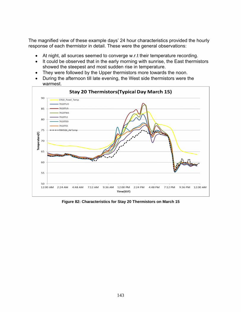
The magrespons

A It

s T D

w

gnified viewe of each t

At night, all st could be ohowed the

They were foDuring the awarmest.

Fig

w of these ehermistor in

sources seobserved thsteepest aollowed by

afternoon til

ure 82: Char

example dan detail. Th

emed to coat in the eand most suthe Upper l late eveni

racteristics f

143

ays’ 24 hourese were th

onverge w.rarly morningdden rise inthermistorsng, the We

or Stay 20 Th

r characterihe general

r.t their temg with sunrn temperats more towaest side the

hermistors o

istics providobservatio

mperature reise, the Easure. ards the normistors we

on March 15

ded the houns:

ecording. st thermisto

oon. ere the

urly

ors

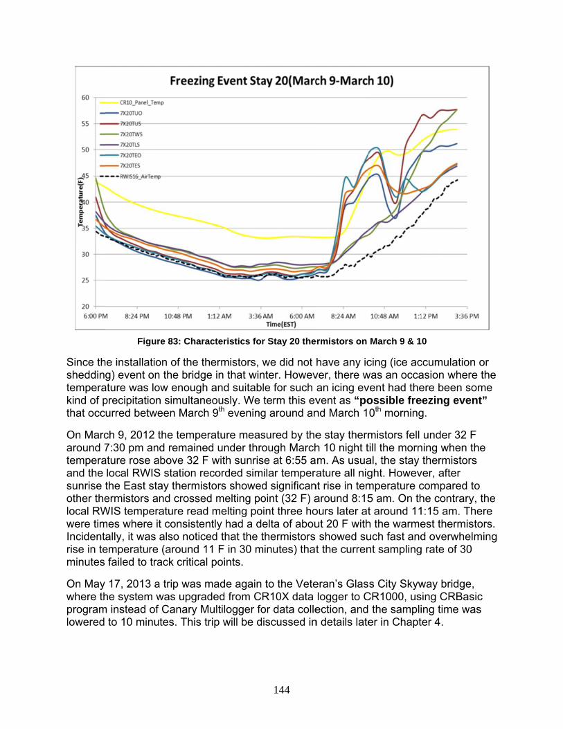
Since thsheddintemperakind of pthat occ

On Marcaround 7temperaand the sunrise tother thelocal RWwere timIncidentrise in teminutes

On May where thprogramlowered

Figur

he installatiog) event on

ature was loprecipitationurred betwe

ch 9, 2012 7:30 pm anature rose alocal RWISthe East staermistors a

WIS tempermes where i

ally, it was emperature

failed to tra

17, 2013 ahe system w

m instead ofto 10 minu

re 83: Charac

on of the thn the bridgeow enough n simultaneeen March

the tempernd remainedabove 32 F S station recay thermistnd crossed

rature read t consistenalso notice (around 11ack critical

a trip was mwas upgradf Canary Muutes. This tr

cteristics for

ermistors, we in that winand suitabl

eously. We 9th evening

rature measd under throwith sunriscorded simtors showedd melting pomelting potly had a de

ed that the t1 F in 30 mpoints.

made again ded from CRultilogger forip will be d

144

r Stay 20 the

we did not nter. Howevle for such term this ev

g around an

sured by theough March

se at 6:55 ailar temperad significanoint (32 F) aint three hoelta of abouthermistors inutes) that

to the VeteR10X data or data colleiscussed in

ermistors on

have any icver, there wan icing evvent as “pond March 1

e stay thermh 10 night t

am. As usuaature all nig

nt rise in temaround 8:15ours later atut 20 F withshowed su

t the curren

eran’s Glaslogger to Cection, and

n details late

March 9 & 1

cing (ice acwas an occavent had theossible fre0th morning

mistors fell till the mornal, the stay ght. Howevmperature c5 am. On tht around 11h the warmeuch fast andnt sampling

s City SkywCR1000, us the samplier in Chapt

0

ccumulationasion whereere been so

eezing eveng.

under 32 Fning when tthermistors

ver, after compared the contrary1:15 am. Thest thermisd overwhel

g rate of 30

way bridge,sing CRBasing time water 4.

n or e the ome nt”

F he s

o y, the here tors. ming

sic as

Section

Leaf Wenearby ldielectricamounts

SectionLWS-L

Aim: Todetermin

ApparatCR1000

Operatiapproximwater andependesends a turn is d

ExperimprovidedCRBasicper minu

n 6.3: LWS

etness senseaves. Thec constant s of water o

n 6.3.1: LabLeaf Wetne

o measure one appropri

tus: LWS-L0 (1), Serial

ng principmately 1cmnd ice are ment on the pmillivolt sigependent o

ment: The led switched c Editor whute.

S-L Dielectr

sors have be LWS-L meof the sens

or ice.

Figure 84

boratory exess Senso

output voltaiate thresho

L Dielectric to USB Int

le: The LWm above the much highepresence ofgnal proporon the prese

eaf wetnesexcitation vere output

ric Leaf We

been develoeasures the

sor’s upper

: Leaf Wetne

xperiment or.

age of the leold for wetn

Wetness Sterface (1),

WS-L measuupper surfr than air, sf moisture ortional to theence of mo

s sensor wvoltage of 2voltage wa

145

etness Sen

oped to estie leaf surfasurface. Th

ess Sensor fu

on measur

eaf wetnessness conditi

Sensor (1), PC, Logge

ures the dieface of the sso the measor frost on te dielectric

oisture or fro

as connect2.5mV. The as set to be

nsor

imate by infce wetnesshe sensor is

unctional dia

rement of

s sensor foions.

Campbell Sernet Softwa

electric conssensor. Thesured dielethe sensor measurem

ost on its su

ted to the Cprogram wrecorded w

ference thes by measus able to de

agram

output vol

r a fixed ex

Scientific Dare.

stant of a ze dielectric

ectric constasurface. Th

ment of the zurface.

CR1000 datwas written with a scan

e wetness ouring the etect minisc

ltage using

xcitation and

atalogger

zone constant o

ant is stronhe sensor zone, which

talogger anin Campberate of onc

of

cule

g

d

of gly

h in

d ell's ce

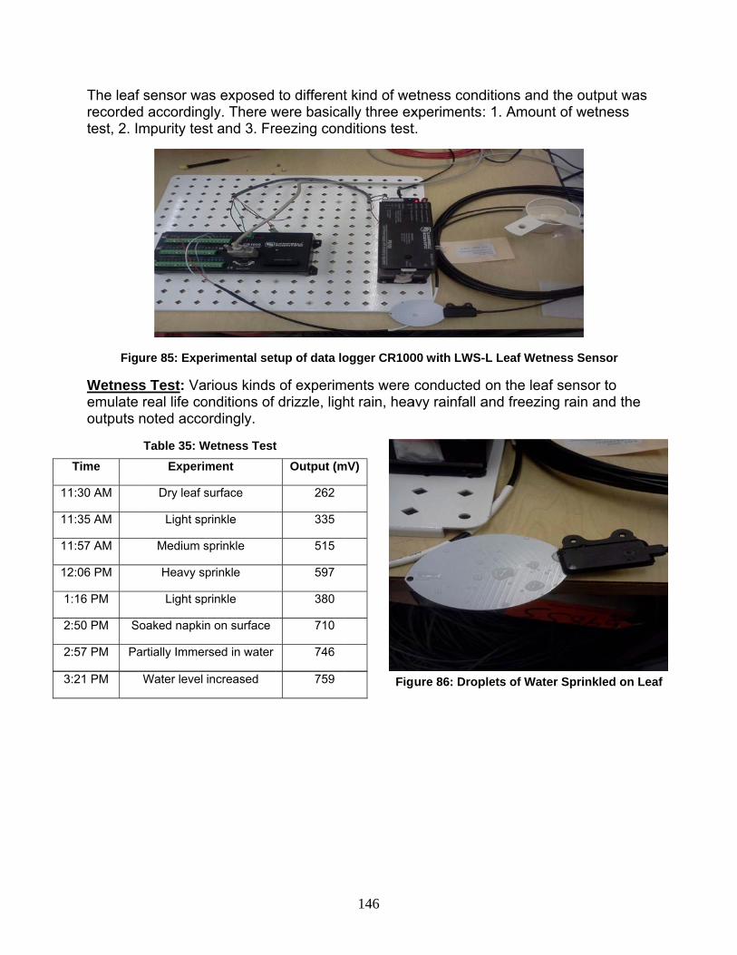
11

11

11

12

1

2

2

3

The leafrecordedtest, 2. I

Fig

Wetnesemulateoutputs

Time

1:30 AM

1:35 AM

1:57 AM

2:06 PM

:16 PM

2:50 PM S

2:57 PM Pa

3:21 PM

f sensor wad accordingmpurity tes

ure 85: Expe

s Test: Va real life conoted acco

Table 35: W

Experim

Dry leaf s

Light sp

Medium s

Heavy sp

Light sp

Soaked napkin

artially Immer

Water level

as exposed gly. There wst and 3. Fre

erimental set

rious kinds onditions of ordingly.

Wetness Test

ment

surface

prinkle

sprinkle

prinkle

prinkle

n on surface

rsed in water

increased

to differentwere basicaeezing con

tup of data lo

of experimdrizzle, ligh

t

Output (m

262

335

515

597

380

710

746

759

146

t kind of weally three exditions test

ogger CR100

ments were ht rain, hea

mV)

Fig

etness condxperimentst.

00 with LWS-

conducted avy rainfall a

ure 86: Drop

ditions and : 1. Amoun

-L Leaf Wetn

on the leafand freezin

plets of Wate

the output t of wetnes

ness Sensor

f sensor to g rain and

er Sprinkled o

was ss

the

on Leaf

11

11

2

3

410

Time

1:00 AM I

1:05 AM

2:05 AM

Time

3:45 PM

:40 PM- 0:30 AM

I

Table 36: Im

Experi

mmersed in c

Salt added

Dry napkin o

Table 37: Im

Experi

Dry leaf kep

mmersed in c(inside fr

mpurity Test

ment

cup of water

d to water

on surface

mpurity Test

ment

t in freezer

cup of water reezer)

t

Output (m

788

1030

264

t

Output (m

262

298 - 30

147

mV)

mV)

00

Figure 87: Lcup of wate

Figure 88:freeze

LWS-L partiaer

LWS-L imm

ally immerse

mersed in cup

d in

p left to

Figur

Figure 89:

re 90: LWS F

148

LWS Wetnes

reezing Tem

ss Test

mperature Tesst

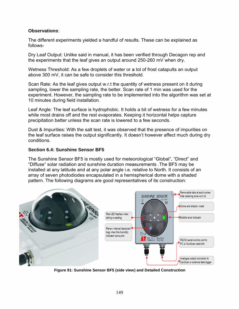
Observa

The diffefollows-

Dry Leafthe expe

Wetnessabove 3

Scan Rasamplingexperim10 minu

Leaf Angwhile moprecipita

Dust & Ithe leaf condition

Section

The Sun“Diffuse”installedarray of pattern.

ations:

erent exper

f Output: Ueriments tha

s Threshold00 mV, it c

ate: As the g, lower theent. Howevtes during f

gle: The leaost drains oation better

mpurities: Wsurface raisns.

n 6.4: Suns

nshine Sens” solar radia

d at any latitseven phoThe followi

Figure

riments yiel

nlike said inat the leaf g

d: As a few an be safe

leaf gives oe sampling ver, the samfield installa

af surface isoff and the runless the

With the sases the out

hine Sens

sor BF5 is ation and stude and attodiodes ening diagram

91: Sunshine

ded a hand

n manual, igives an ou

droplets ofto conside

output w.r.t rate, the be

mpling rate ation.

s hydrophorest evaporscan rate i

alt test, it watput signific

or BF5

mostly usedunshine dut any polar ncapsulated

ms are good

e Sensor BF

149

dful of resul

t has been utput around

f water or ar this thresh

the quantitetter. Scan to be imple

obic. It holdsrates. Keepis lowered t

as observedantly. It doe

d for meteouration meaangle i.e. rd in a hemid represent

F5 (side view

lts. These c

verified thrd 250-260

a lot of frosthold.

ty of wetnesrate of 1 m

emented int

s a bit of weping it horizto a few se

d that the pesn’t howev

orological “Gasurementsrelative to Nspherical dtatives of its

) and Detaile

can be expl

rough DecamV when d

t catapults a

ss present min was useto the algor

etness for azontal helpsconds.

presence ofver affect m

Global”, “Di .The BF5 m

North. It condome with as constructi

ed Construct

lained as

agon rep andry.

an output

on it duringed for the rithm was s

a few minuts capture

f impurities much during

irect” and may be nsists of an a shaded ion:

tion

nd

g

set at

tes

on g dry

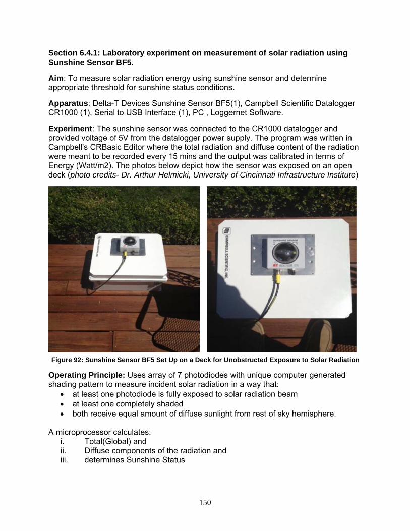
SectionSunshin

Aim: Toappropri

ApparatCR1000

ExperimprovidedCampbewere meEnergy (deck (ph

Figure 9

Operatishading

a a b

A microp

i. ii. iii.

n 6.4.1: Labne Sensor

o measure siate thresho

tus: Delta-T0 (1), Serial

ment: The sd voltage ofell's CRBaseant to be r(Watt/m2). hoto credits

92: Sunshine

ng Princippattern to t least one t least one oth receive

processor cTotal(GloDiffuse cdetermin

boratory exBF5.

solar radiatold for suns

T Devices Sto USB Int

sunshine sef 5V from th

sic Editor whrecorded evThe photos

s- Dr. Arthu

e Sensor BF5

ple: Uses armeasure inphotodiodecompletely

e equal amo

calculates: obal) and componentsnes Sunshin

xperiment

ion energy shine status

Sunshine Sterface (1),

ensor was che datalogghere the totvery 15 mins below depr Helmicki,

5 Set Up on a

rray of 7 phncident solae is fully exy shaded ount of diffu

s of the radne Status

150

on measur

using sunss conditions

Sensor BF5PC , Logge

connected tger power stal radiation

ns and the opict how theUniversity

a Deck for Un

hotodiodes ar radiation posed to so

use sunlight

iation and

rement of

shine sensos.

5(1), Campbernet Softw

to the CR10supply. Then and diffusoutput was e sensor waof Cincinna

nobstructed

with uniquein a way th

olar radiatio

t from rest

solar radia

or and dete

bell Scientifware.

000 datalog program w

se content ocalibrated as exposedati Infrastru

Exposure to

e computerhat: on beam

of sky hem

ation using

rmine

fic Datalogg

gger and was written of the radiain terms of d on an ope

ucture Institu

o Solar Radia

r generated

misphere.

g

ger

in ation

en ute)

ation

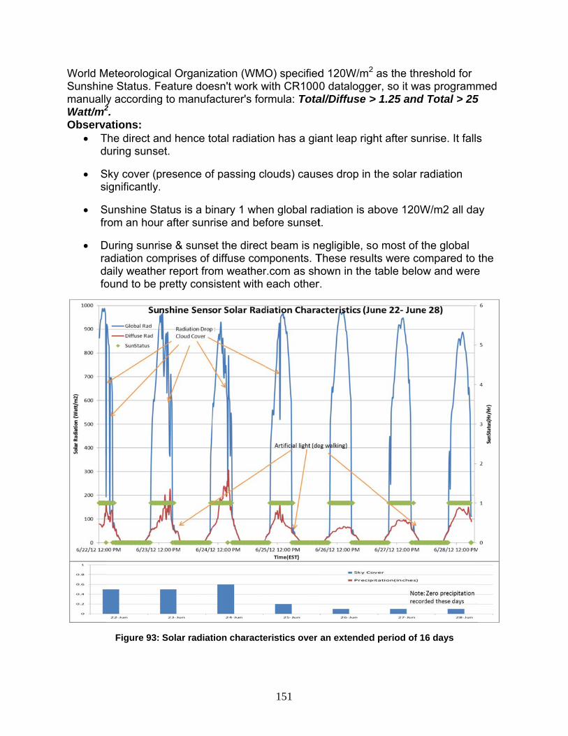
World MSunshinmanuallyWatt/m2

Observa T

d

Ss

Sfr

Dradfo

Meteorologicne Status. Fy according2. ations:

The direct auring sunse

Sky cover (pignificantly.

Sunshine Strom an hou

During sunriadiation comaily weatheound to be

Figure 93:

cal OrganizFeature doeg to manufa

nd hence toet.

presence of.

tatus is a bir after sunr

ise & sunsemprises of er report fropretty cons

Solar radiat

zation (WMOesn't work wacturer's for

otal radiatio

f passing cl

inary 1 wherise and bef

et the directdiffuse com

om weathersistent with

tion characte

151

O) specifiedwith CR100rmula: Tota

on has a gia

louds) caus

en global rafore sunset

t beam is nmponents. Tr.com as sheach other

eristics over

d 120W/m2

0 dataloggeal/Diffuse >

ant leap rig

ses drop in

adiation is at.

egligible, sThese resuhown in the r.

an extended

2 as the threer, so it wa> 1.25 and

ght after sun

the solar ra

above 120W

o most of thlts were cotable below

d period of 1

eshold for s programmTotal > 25

nrise. It falls

adiation

W/m2 all da

he global mpared to w and were

6 days

med 5

s

ay

the e

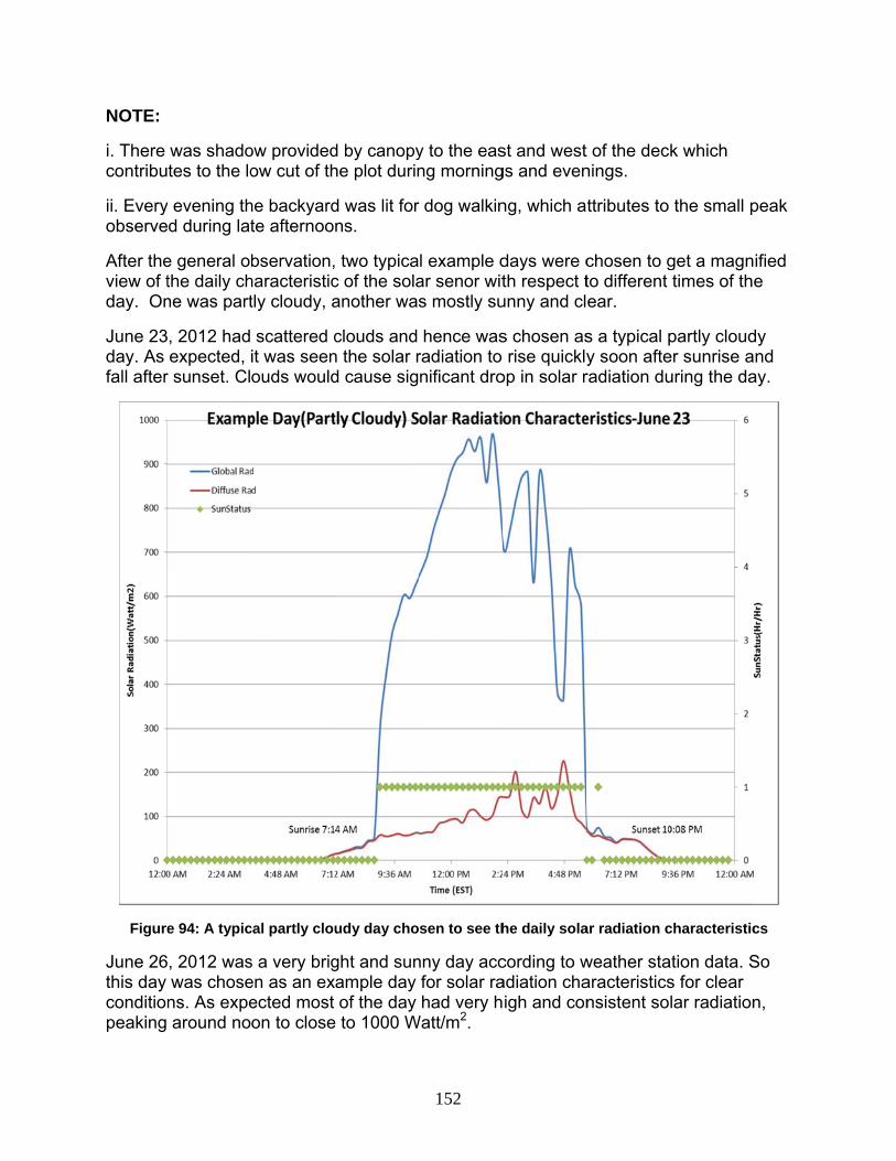
NOTE:

i. There contribu

ii. Everyobserve

After theview of tday. On

June 23day. As fall after

Figure

June 26this day conditionpeaking

was shadotes to the lo

y evening thd during lat

e general obthe daily chne was part

, 2012 had expected,

r sunset. Cl

e 94: A typic

, 2012 waswas chose

ns. As expearound no

ow providedow cut of th

he backyardte afternoo

bservation,haracteristictly cloudy, a

scattered cit was seenouds would

cal partly clou

s a very brigen as an exected most on to close

d by canopyhe plot durin

d was lit forns.

two typicac of the solaanother was

clouds and n the solar rd cause sig

udy day cho

ght and sunample day of the day

e to 1000 W

152

y to the easng morning

r dog walkin

l example dar senor wits mostly su

hence wasradiation to nificant dro

sen to see th

nny day accfor solar rahad very h

Watt/m2.

st and westgs and even

ng, which a

days were cth respect tunny and cl

s chosen asrise quickly

op in solar r

he daily sola

cording to wadiation chaigh and con

t of the decknings.

ttributes to

chosen to gto different ear.

s a typical py soon afteradiation du

ar radiation c

weather staaracteristicsnsistent sol

k which

the small p

get a magntimes of the

partly clouder sunrise auring the da

characteristic

ation data. Ss for clear lar radiation

peak

ified e

dy nd

ay.

cs

So

n,

Figcha

Section

Introducbucket. switch inadjustabscreen oand hasmoisturethermos

ure 95: A typaracteristics

n 6.5: Met O

ction: The Rain is metnside the buble feet to eon the funn Santoprene. The rain stat based h

pical clear su

One Rain T

Met One Rtered into aucket whichensure propel that prev

ne rubber cacollected is

heater insid

unny day tak

Tipping Buc

Rain or Heaa collection h tips for eaper mountinvents debrisable jacket s dischargede that can

153

ken as examp

cket

ated Snow Gfunnel on t

ach 0.01 incng with bracs from cloggfor better r

ed through tmelt snow

ple to see the

Gage is a dtop of the bch precipitacket CM240ging. The cresistance tthe rain gaginto water b

e daily solar

dual chambucket. Ther

ation collect0. There is cable lengthto UV degrage base. Thbefore mea

radiation

ered tippingre is a mercted. It has a primary

h is forty feeadation andhere is a asurement.

g cury

et d

Figure

SectionTipping

Aim: Todetermin

ApparatScientifi

Operatirain intothermoseq., the A momepulse ch

The

96: Rain Tip

n 6.5.1: Labg Bucket

o measure pne appropri

tus: MetOnc Datalogg

ng Princip tipping buc

statically cotipping buc

entary contahannel. Wat

tipping qua

Tip

pping Bucket

boratory ex

precipitationiate samplin

ne Rain Tiper CR1000

ple: Collectscket. Snowfntrolled hea

cket assemact closure ter drains o

antity is dete

to in3: Catc

t (from top le

xperiment

n amount ung rates an

ping Bucke (1), Serial

s rainfall in fall captureating elemebly tips duefor each in

out base of

ermined bygiven

Met One C

ch orifice ar

= 113=

154

eft clockwise

on measur

sing Met Ond threshold

et (1), 100 mto USB Inte

the 12 inched in collectent. For evee to gravity crement ofthe gage a

y the equivasurface are

Conversion

rea (πd2/4)

3.04 X 0.01 = 18.52 ml

e) distant view

rement of

One Rain Tid for condit

mL Gesslererface (1),

h collection tion funnel aery 0.01 incand activat

f rainfall is rafter tipping

alent volumea. Factor:

) X increme

in3

w, top view a

precipitati

pping Buckions.

r Buret (1), PC, Logge

funnel andand melted

ches of raintes a mercurecorded by.

me of liquid c

ent in inches

and inside vi

on using

ket and

Campbell rnet Softwa

d meters thed by n/snow-wateury reed swy datalogge

collected in

s

iew

are.

e

er witch. er

n a

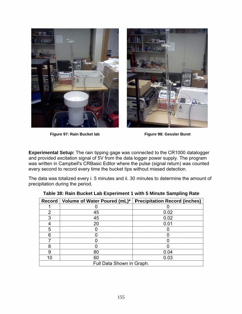
Experimand provwas writevery se

The dataprecipita

T

Re

Figure 97

mental Setuvided excitatten in Camecond to rec

a was totaliation during

Table 38: R

ecord Vo1 2 3 4 5 6 7 8 9

10

: Rain Bucke

up: The raiation signal

mpbell's CRBcord every

ized every g the period

Rain Bucke

lume of W

et lab

n tipping gal of 5V fromBasic Editotime the bu

i. 5 minutesd.

et Lab Expe

Water Poure0

45 45 20 0 0 0 0

80 60 Full Data

155

age was com the data loor where theucket tips w

s and ii. 30

eriment 1 w

ed (mL)* P

Shown in G

Figure 9

onnected toogger powee pulse (sig

without miss

minutes to

with 5 Minu

Precipitatio

Graph.

98: Gessler B

o the CR100er supply. Tgnal return)sed detectio

determine

ute Sampli

on Record0

0.02 0.02 0.01

0 0 0 0

0.04 0.03

Buret

00 dataloggThe program was counton.

the amoun

ing Rate

d (inches)

ger m ted

nt of

Ta

Re

It has beeach tip marginathe funnslow/inteconsider18.53 m

Section

The 087vibrating

able 39: Ra

ecord Vo1 2 3

een observe= 18.53 m

ally more thanel. The resermittent pared a thres

ml of water.

Figure 9

n 6.6: Good

72F1 Goodrg tube and c

ain Bucket

lume of W

ed that the l of water. Dan that tippult obtained

assage of whold check

99: Rain Buc

drich Ice De

rich Ice Detcommunica

t Lab Expe

Water Poure40

200 300

device folloDuring the fped out, becd is fairly cowater into th

for precipit

cket accurac

etector

tector detecates the ass

156

eriment 2 w

ed (mL)* P

ows the facfirst few reacause of adonsistent irrhe bucket utation in the

cy experimen

cts ice accusociated fre

with 30 Min

Precipitatio

ctory calibraadings the qdhesion wherespective

using the bue algorithm

nt (actual vs t

umulation oequency ch

nute Sampl

on Record0.02 0.1

0.16

ation standaquantity of ere some wof fast/cont

uret. One tipas each tip

tipping volu

on an ultrashanges thro

ling Rate

d (inches)

ards whereliquid let in

water stickstinuous or p can be p equals to

me)

sonic axiallyough an RS

e is

s to

y -232

or digitaoperate

The 087an Outp

Sectionusing G

Aim: Tosampling

Apparat(1), CamLoggern

Operatitransitioexposedconditionfrequenccommunlinear re

l current loocontinuous

72F1 consisut Interface

Figure 1

n 6.6.1: LabGoodrich Ic

o measure ig rates and

tus: 0872Fmpbell Sciennet Software

on Principns between

d to the envns causing cy in an ultrnicated throelationship):

Ic

op data linksly in an ou

sts of four fue CCA, a Fi

100: The Goo

boratory exce Detecto

ce thicknesd de-icing th

F1 Ice Detecntific Dataloe.

ple: The Gon solid and vironment. Ichange in

rasonic axiaough data li:

ce Thicknes

k. The 0872tdoor enviro

unctional asilter assem

odrich Ice De

xperiment r 0872F1

ss using Gohreshold.

ctor (1), Micogger CR10

oodrich Ice liquid stateIce builds uits mass. Tally vibratinnk. Ice Thic

ss = -0.000

157

2F1 is mounonment.

ssemblies: bly, and a S

etector (exte

on measur

oodrich Ice

croCare An000 (1), Se

Detector 08es. It consisup on this eThis mass cng tube. Theckness is c

015*Freque

nted on a p

a Main circStrut and P

ernal and fun

rement of

Detector a

nti-Stat Spraerial to USB

872F1 measts of a senslement whechange caue associate

calculated a

ency + 6 (in

pole and is

cuit card asProbe assem

nction diagra

ice presen

nd determi

ay (1), SlidiB Interface (

asures precsing elemeen it is expouses a shifted frequencas (manufac

n inches)

designed to

ssembly (CCmbly.

ams)

nce/thickne

ne appropr

ing Calipers(1), PC,

cipitation nt that is osed to icint in vibrationcy changes cturer-spec

o

CA),

ess

riate

s

ng n are

cified

158

Experimental Setup: The ice detector was connected to the CR1000 datalogger and provided signal of 115V from the mains power supply. The program was written in Campbell's CRBasic Editor where the frequency of the probe was counted every minute. The data was recorded every 1 minute to determine the corresponding amount of ice thickness.

FigExp

F

ObservarelationsThe thre

ure 101: Ice periment

igure 103: Pr

ation: The ship betweeeshold to tri

Detector Mo

robe before S

device folloen change gger de-ici

ounted for

Spraying

ows the facin frequencng cycle wa

159

Figure

ctory calibracy and correas set at 0.0

102: Microc

Figure 104:

ation basedesponding c04 inches a

are Anti-Stat

Probe After

d on the spechange in iand it prove

t Freezing Sp

Spraying

ecified lineace thicknes

ed to be ab

pray

ar ss. le to

de-ice ththe probminutes

The samdeterminice thickthicknesdue to q

Figure 1

ProbeCaliper Zero Re

= 0000

he probe cobe remains .

mpling rate ning presenkness. This ss of ice forquick ice me

105: Frequen

e ThicknessTest (inche

eading (no ic0.2425

0.2500 0.2550 0.2580 0.2650

T

ww

ro

ompletely dwarm) than

chosen wance of ice. Awas done ming on proelting of thin

ncy/Ice thickn

Table 40: C

s es)

DelThickn

ce)

The thicknemeasured ithout the icwere erraticoom tempe

fit onto the

uring the hn the heat-t

s 1 minute An experimin order to obe and than layer of ic

ness charact

Caliper Test

lta for Ice ness (inches

0

0.075 0.125 0.155 0.225

ess (diameteusing slidince coating. c as: The icerature and e ice layer w

160

eating timeime and ke

and it provent was runmanually dat measurece.

teristics of 0

t

s) Sensor

Ice (i

0.00.00.00.0

er) of the png calipers w

The resultsce melted tothe caliperwithout sha

e. The de-iceeps the pro

ved to be qun using slidetermine th

ed by senso

0872F1 durin

r Data for nches) 0

0187 0254 0305 0297

robe was with and s obtained oo fast at rs couldn't aving it.

cing cycle laobe frost-fre

uite effectivding caliperhe relationsor, but it wa

ng freezing sp

Figmeasu

asts longer ee for a cou

ve in rs to measuship betweeasn't effectiv

pray experim

ure 106: Thicurement usin

(as uple

ure en ve

ment

ckness ng calipers

161

Initial results:

The chief motivation behind lab experimentation of the different sensors was to find a meaningful conversion of the parameters recorded by the different sensors into comprehensive values, and also to test and calibrate them, if necessary.

The following table is a summary report of the behavior of the new icing sensors.

Table 41: Icing Sensors Initial Observations

Sensors Observations Stay Thermistors All stay thermistors measure temperature in unison at night. Solar

radiation (daytime) causes sufficient spread in temperature recorded depending upon thermistor location. RWIS air temperature can have a delta of about 20 F during sunrise.

Ice Detector The vibration frequency decreases with increased mass of ice on sensor probe. Correctly determines ice thickness as verified with calipers.

Solar Sensor The direct, and hence, total radiation has a giant leap right after sunrise. It falls dramatically during sunset. Sky cover (presence of passing clouds) causes drops in solar radiation significantly. Sunshine Status is usually above 120 W/m2 (WMO threshold) all day from an hour after sunrise and before sunset.

Rain Bucket The device follows the factory calibration standards where each tip = 18.53 mL of water or 0.01 inches of rainfall.

Leaf Wetness The leaf gives an output around 260-270 mV when dry. It gives an output of ~ 300 mV when it is frosted and higher when there is rainfall or snow.


Laboratory experiments have documented and verified the proper operation and calibration of a new sensor suite to be deployed on the VGCS bridge. These include:

Geokon Thermistor 3800-2-2, for stay surface temperatures

LWS-L Dielectric Leaf Wetness Sensor, for detecting water/moisture with some classification as ice, light rain/snow, or heavy snow/rain.

Sunshine Sensor BF5, for detecting and quantifying solar radiation and approximate level of cloud cover

Met One Rain Tipping Bucket, for detecting and quantifying precipitation

Goodrich Ice Detector, for detecting and quantifying ice thickness

Chapte

Section

An icingin order regardlescale shinitial exVGCS coperatiodeicing f

When thicing winanti/deic

Section

Scott Pa

For desiinformatdata to mpropertieinformatbridge isinitially o10ft longstays hacampustaken fro

er 7: Field

n 7.1: Introd

experimento better un

ess of the nheath specimxperiments could be reponal, the VGfluid tests a

he weather nd tunnel. cing fluid.

n 7.2: Desig

ark Setup

igning an eftion neededmake an aces of the shtion about cs inefficient operated dug with the save been se. Figure 10om Google

d Study o

duction

nt station wanderstand tatural precmens weredemonstratplicated on GCS experimand heating

was warm,Experiment

gn of Icing

and Backg

ffective lond to be gathccurate therheath, inforcoating and

and dangeuring the wisame diameet up on the7 shows a Earth.

Figure 10

of Tempe

as set up athe nature oipitation an

e used for eted that icinthe stay spments carri

g tests.

, experiments performe

Experime

ground

g term anti-hered. The rmal modelmation abo

d internal heerous. An icinter of 201eter, materiae outdoor coscreen sho

07: Google Ea

162

rature Ef

at the Univeof icing eved minimizexperiments

ng and shedpecimens. Aied out inclu

nts were caed in the ici

nt Station

-icing/deicininformation of cable st

out efficacy eating. Perfcing experim2-2013. Thal, and refleoncrete pad

ot of the con

arth Screens

ffect on S

ersity of Toleents, condu the risk to

s in the wintdding similaAfter the exuded senso

arried out inng wind tun

ng technolon required intays, determof chemica

forming thement stationhree full scaective brusd at Univerncrete pad

shot of Scott

Scott ParkConcrete

Stay Shea

edo’s Scottct icing exppersonnel.

ter of 2012-ar to that obxperiment sor studies, c

n the Univernnel include

ogy for VGCncludes themining the tals on the sese experimn was desigale sheathinhed surface

rsity of Toleat Scott Pa

t Park

k’s Pad

aths

t Park Camperiments . Three full-2013. The bserved onstation was coating tes

rsity of Tolee coating a

CS, more e following: thermal

stays, and ments on thegned, built ng specimee as the VG

edo Scott Paark which is

mpus

n the ts,

edo nd

e and

ens GCS ark

s

On the bdependiused. Asat top ofspecimecontainssimulate

Data Ac

The spethe sheaoutside Additioninside tedetermincollect thsnow wesensors icing beh

bridge the sng on the los shown in f the cross-en due to sas north facine the bridge

cquisition S

ecimens weath surfaceand inside

nally, photo emperature ne the diffehe ambientere used thwhich were

havior of sp

stays have ocation of sFigure 79, section. In afety reasong, south fae conditions

System an

re instrume, which conthe sheath sensors toof the spec

rence betwt temperaturoughout the installed opecimen.

Figure 108:

82 to 156 pstays. In theon the bridthe test conns. As showacing, and hs as realistic

nd Sensor S

ented with dnsist of an a

in order to track sun l

cimen at difween liquid w

re, wind sphe outdoor on the uppe

163

Experimenta

prestressinge test set uge at mid-snfiguration,wn in Figurhorizontal scally as pos

Setup

designed tharray of flat

get surfaceocation, a pfferent locawater and i

peed, wind dexperimenter part and

al Setup

g epoxy coap, 120 un-tspan, the e, the strandre 108, the specimens ssible.

hermistors tthermocou

e temperatuprobe therm

ations, an ace, and a lodirection, ats. Figure 1east side o

ated structutensioned spoxy coate

ds rest at thexperimentoriented no

to get the teuples installure of specmocouple forray of ice docal weathe

and amount109 shows of the speci

ural strandsstrands wered strands ae bottom oftal setup orth-south t

emperatureled both cimen. or getting thdetectors toer station tot of rain andseveral imen to mo

s re are f the

to

e at

he o o d

onitor

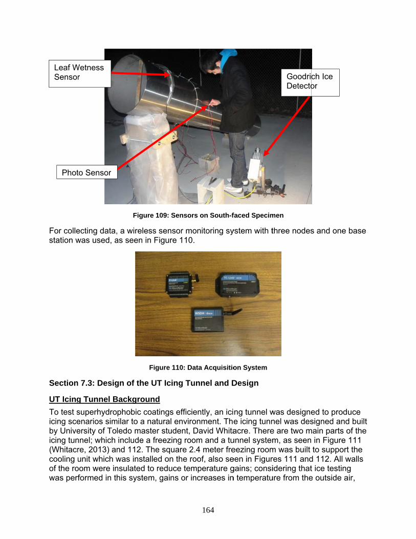
For collestation w

Section

UT Icing

To test sicing sceby Univeicing tun(Whitacrcooling uof the rowas perf

Leaf WSensor

Phot

ecting data,was used, a

n 7.3: Desig

g Tunnel B

superhydroenarios simersity of Tonnel; which re, 2013) anunit which w

oom were informed in t

Wetness r

to Sensor

Figure

, a wirelessas seen in F

Fig

gn of the U

Background

phobic coamilar to a na

ledo masteinclude a fnd 112. Thewas installensulated to his system,

109: Sensors

s sensor moFigure 110.

gure 110: Da

UT Icing Tu

d

atings efficieatural enviroer student, Dreezing rooe square 2.ed on the roreduce tem, gains or in

164

s on South-f

onitoring sy

ata Acquisitio

unnel and D

ently, an icionment. TheDavid Whitaom and a tu.4 meter freoof, also semperature gncreases in

faced Specim

ystem with t

on System

Design

ng tunnel we icing tunnacre. Thereunnel systemeezing roomeen in Figurgains; consin temperatu

men

three nodes

was designenel was dese are two mm, as seen

m was built res 111 andidering that

ure from the

GoodriDetecto

s and one b

ed to produsigned and

main parts o in Figure 1to support

d 112. All wt ice testinge outside ai

ch Ice or

base

uce built

of the 111 the

walls g r,

Freez

Co

Free

C

which isnot desilow as -2travel thinstalledexperimsuitable light win°C), etc.object m

zing Room

ooling Unit

ezing Room

Cooling Unit

significantred. The co20 °C. The rough the t

d inside the ents. Additfor icing to

nds and ver.).The tunne

may be plac

t

ly warmer tooling unit hfreeze roo

tunnel systetunnel systionally, tem be achievey cold tempel system a

ced in order

Figure 111:

than the cirhas the capm has an oem as a clotem for the

mperature wed (i.e. highperatures (-also includer for experim

: SolidWorks

Figure 112

165

rculating airpability to moutlet and inosed loop sy

user to be was adjustah winds and-20 °C), hig

ed a test sements to be

s Design for t

2: UT Icing T

r within the maintain a cnlet to allowystem. A mable to adjble, thus, ad very cold gh winds anction, which

e performed

the UT Icing

Tunnel

icing tunneconstant temw the supercmulti-speed just wind spallowing vartemperatur

nd cold temh is the ared.

Tunnel

el system, amperature acool air to fan was peed duringrious conditre (-20 °C),perature (-

ea where an

Tunnel Sys

Test Sectio

Tunnel Sy

Test Sect

are as

g tions 10 n

stem

on

ystem

tion

Test Se

This secThis testalso inclpresente

Misting

The icinsystem. get blowthe specresemblsection rthat are pressurepreviousas -20 °Cice accrespecime0.012, 0perform to each The nozThe resuof appro

ction

ction consist section alludes a mised below.

System

g tunnel caThis system

wn onto the cimen at a pes field conroughly X , hooked up

e. . The missly mentionC. This alloetion is allo

en. The mis0.014, or 0.0

experimennozzle is b

zzles were tult shows thoximately 50

sts of a 30 clows users

sting system

Figure 11

an create bom uses noztesting spe

proper distanditions, theas seen in to standar

sting array sed, the icin

ows the testowed to occsting system016 inch or

nts with diffeetween 0.0tested for dhat 0.012, 00, 40, and 4

cm diameteto take pic

m, camera,

13: Testing S

oth rime anzzles to proecimen at vance to alloe misting syfigure 114

rd city wateseems to c

ng tunnel is ting object acur when thm allows therifice. Havinerent drople007 and 0.0roplet size 0.014, and 42 microme

166

er optically ctures of a sand specim

Section of the

d glaze typoduce a fineariable spe

ow the wateystem was. The setupr, which is aover the tesdesigned tand water de droplets c

e user to chng different et sizes and011 gallons

using Parti0.016 inch

eters (micro

clear tube aspecimen dmen mounti

e UT Icing Tu

pes of ice bye mist, veryeeds. In order droplets tinstalled in

p consists oadequate bst section dto decreasedroplets to contact the

hange the nnozzle size

d flow ratesper minute

icle Image Vorifice nozz

on), respect

as shown induring an exing systems

unnel

y the use oy small wateder for the to freeze in

n front of theof three misbecause it odiameter ade in temperabe superco

e surface ofnozzle size es allows ths. The flow e (gpm). (WVelocimetryzle distributively.

n Figure 11xperiment. s, which wi

of a misting er droplets mist to reac

n a manner e testing sting nozzleoperates in dequately. Aature to as ooled, and tf the testingto either a

he user to rate associ

Whitacre 201y (PIV) mettes droplet

3. It ll be

that ch that

es low

As low

thus, g

iated 13) thod. size

Camera

A PanasFigure 1maintaineliminateon the te115 hasThe camcan be ito be struser to c(Panaso

Mountin

Additiontesting smountinwell as a

a System

sonic HX-A14, to allow

ns roughly tes any difficesting secti a high defi

mera does nnstalled onreamed to tcontrol recoonic 2013)

Fi

ng System

nally, locatespecimen tog system aa dial to cha

Figure 11

100D camew the user tthe same teculty in takion tube froinition 1080not have a v a smartphthe device iording, take

igure 115: Pa

d in the teso be mountalso includeange the an

14: Misting S

era was insto clearly doemperatureing pictures

om the temp0P video revideo screeone or tablet is installed

e pictures, a

anasonic HX

st section ised across ts a load cengle of the

167

System in the

stalled withiocument ea

e as inside ts due to theperature difcorder anden, howeveet. This apd on via Wiand change

X_A100D Cam

s a mountinthe testing s

ell which is uobject durin

e Testing Se

n the testinach experimthe testing se possible fofference. Th is waterpro

er, the Panapplication ali-Fi. The ap

e the setting

mera (Panaso

g system. Tsection as used to detng the expe

ction

ng section, sment. The csection, whormation ofhe camera oof up to 5 asonic Imagllows for a rpplication ags of the ca

onic 2013)

This systemseen in Figtect lift and eriment. Ho

Camera

Misti

shown in camera lenshich ultimatef condensaseen in Figfeet of wat

ge applicatireal time vilso allows t

amera.

m allows a gure 116. T

drag forcesowever, the

a

ng System

s ely

ation gure ter. on deo the

he s as

e

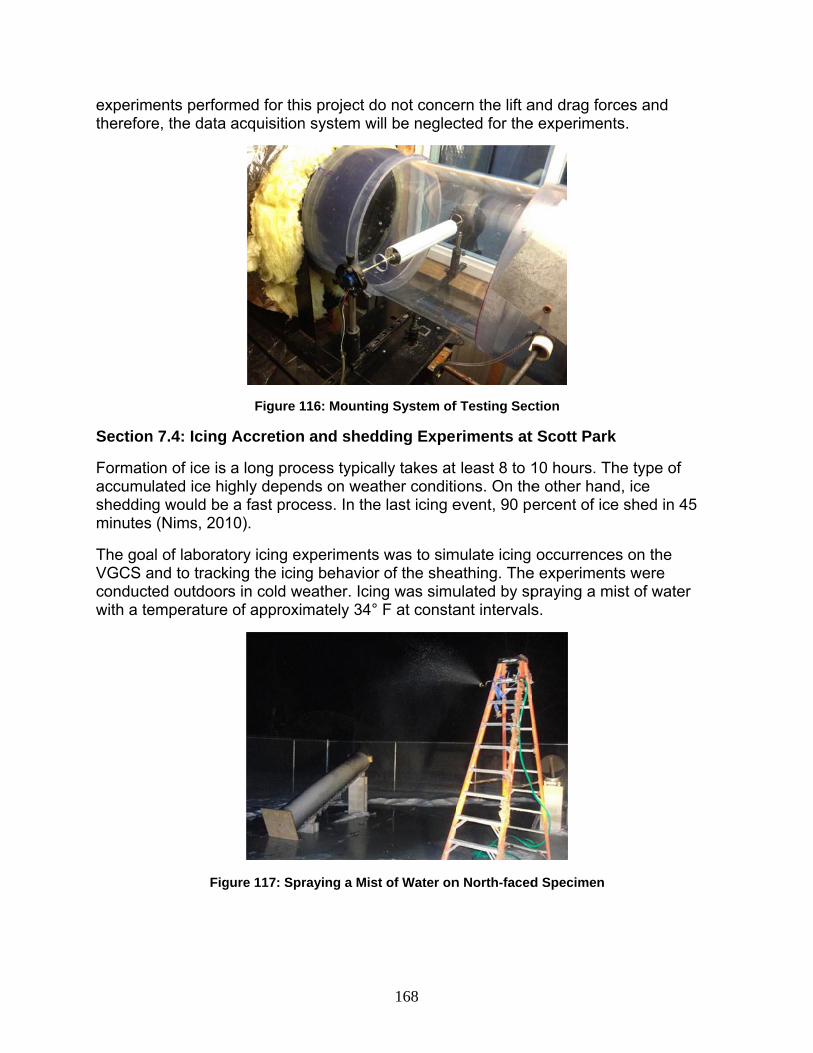
experimtherefore

Section

Formatioaccumusheddinminutes

The goaVGCS aconductwith a te

ents perfore, the data

n 7.4: Icing

on of ice is lated ice hig would be(Nims, 201

al of laboratand to tracked outdoor

emperature

Fig

rmed for thiacquisition

Figure 1

Accretion

a long procghly depen a fast proc10).

tory icing exking the icins in cold weof approxim

gure 117: Spr

s project don system wi

16: Mountin

and shedd

cess typicands on weatcess. In the

xperiments g behavior eather. Icinmately 34°

raying a Mist

168

o not concell be neglec

g System of

ding Expe

lly takes at ther conditi

e last icing e

was to simof the sheag was simuF at consta

t of Water on

ern the lift acted for the

f Testing Sec

riments at

least 8 to 1ons. On the

event, 90 pe

mulate icing athing. Theulated by spant intervals

n North-faced

and drag fore experimen

ction

t Scott Park

10 hours. Te other hanercent of ic

occurrencee experimenpraying a ms.

d Specimen

rces and nts.

k

The type of nd, ice ce shed in 4

es on the nts were mist of wate

45

er

The watdid not rthick acc

Simulatifalling inreports oto happeallows sprove faafter sheambient

As the adue to grequired2011 (S

Presenceliquid wabefore sh

ter was appraise the spcumulation

F

ng sheddinn a fashion of (Belknapen when airolar radiatio

alling criteriaedding. Solt temperatu

F

ambient temgravitationald for sheddiection 3.3.2

e of ter hedding

plied slowly pecimen tem

of ice on th

Figure 118: P

ng was tricksimilar to s

p, 2011), (Jor temperatuon to warma and to crear radiationres and cau

Figure 119: W

mperature inl loading. Icng of an ice2). Figure 1

enough thamperature ahe north fac

Pattern of Ice

kier than thahedding thaones, 2010ure is above

m up the speeate a basen makes a duses liquid

Water benea

ncreases abcing experime layer. Thi20 shows t

169

at the wateabove freezcing specim

e Accumulati

at of formatat occurs o

0), and (Nime freezing aecimens. Theline of spedramatic difwater to fo

th the Ice La

bove freeziments haves is consistthe steps o

r and latenzing. Figure

men.

ion on Outdo

tion. The taon the bridgms, 2010), icand with a che experim

ecimens’ befference be

orm under th

ayer before S

ng ice fallse shown thatent with an

of shedding

t heat of trae 118 show

oor Tests

arget was toe. Based oce sheddinclear sky. Aents have b

ehavior befoetween spehe ice on th

Shedding

in large cuat at least 1n observed that a large

ansformatiows a ½ inch

o simulate icon the past g is more li

A clear sky been done ore, during,ecimen and he specime

urved chunk/4” thickneicing event

e chunk of

on

ce

kely

to and

en.

ks ss is t in ice

on a staexperim

Figure 1the 18ththe icing

y during siment is on th

21 shows th of Februarg behavior a

mulation exhe VGCS w

the temperary 2013. Asas it occurs

xperiments website.

Figure 120:

ature monits shown in ts on the VG

170

goes throu

Ice Sheddin

toring of sothat figure,

GCS.

gh. A video

ng Steps

outh-faced sthe specim

o of this she

specimen frmen accurat

edding

rom the 15ttely simulat

th to tes

Figure 121st of FAn ice lathicknesfreezing

22 monitorFebruary 20ayer startedss was diffic. Water spr

Figure 121:

Figure 122:

rs the secon013. Part Ad to accumucult due to tray was con

: Stay’s Beha

: Stay’s Beha

nd simulatioA of this figuulate on thethe latent hntrolled dur

171

avior in Icing

avior in Icing

on test whicure focuses e specimeneat which w

ring the acc

g Test – 2/15

g Test – 2/20

ch was donon the ice

n at 21:10. Iwas causedcumulation

5 to 2/18

to 2/22

ne during thaccumulatncreasing t

d by additioprocess to

he 20th to thion scenarithe ice

onal water prevent an

he o.

n ice

172

layer from washing away. The sudden increase and decrease of temperature in part A illustrates the change in specimen temperature when water is applied.

Part B of the graph illustrates ice persistence behavior of the specimen. The outdoor weather temperature was 21° F during the night and stayed below freezing throughout the day.

Part C shows the ice shedding process. The temperature of both the top and the east surface of the specimen increased dramatically at sunrise. The sun was out and solar radiation caused the presence of liquid water between ice layer and specimen. Ice shedding happened at 13:25.

Part D again shows ice accumulation scenario of the specimen. There is a coincidence between part A and D. This demonstrates the consistency of the icing behavior of the specimen.

Monitoring and comparing the data collected during several icing simulation tests show that it is possible to reproduce ice accretion and shedding in the same manner as it occurs on the VGCS at a high confidence level. During February and March 2013, approximately 12 icing events were simulated while no natural icing events occurred (Appendix A).

Section 7.5: Thermal Experiments at Scott Park

Because of the large empty area in the stays, one of the most interesting applicable technologies for the VGCS is internal heating. Designing of heating system requires an accurate thermal model of stainless steel stays. There is simply no way to establish an accurate thermal model of VGCS’s stays without experimentation. The primary uncertainty in the development of the thermal model is the convective heat flow inside a stay section. To examine the basic feasibility of heating, preliminary thermal experiments were carried out on the specimen with the same thermal mass as the VGCS stays.

For the thermal experiments, the pipe was instrumented with flat probe thermocouples to collect temperature in points of interest. Flat thermocouples were installed on beginning, end, and midsection of the pipe’s surface. Three tiny holes were made in the specimen for collecting the inside temperature of the pipe at the specified locations. An anemometer was used for collecting the temperature and air speed of the pipe’s inlet and outlet. Ice detectors were used to distinguish liquid water from ice. A 70,000 BTU forced air space heater was used as a heat source.

On the bIn the teacceptathrough to underflows insstainlessperforma

The goageneral the pipelayer of

H

bridge at mest configurable to havethe sheath

rstand pipeside the pips steel sheaance in the

al of the firsthermal res, and the icice on the s

Heater

Fig

id-span, theation, the s

e the strand is more sig’s response

pe. Thermaath in both deicing str

Figure 124

t thermal exsponse for ce melting pspecimen a

gure 123: The

e epoxy coastrands are s at the botgnificant thae in anti-icinl tests weredeicing and

rategy rathe

4: Strands C

xperimentsthe sheath

pattern. Theand then blo

173

ermal Experi

ated strandat the bottottom of the an convectng and the e conductedd anti-icing.er than anti

Configuration

s was to gaiduring deic

e initial testow hot air in

ment Setup

ds are at theom of the sspecimen ion inside tice accumud to unders. The speci-icing strate

n in Thermal

in a better ucing, how ht included anside the p

e top of thepecimen. Tconsidering

the sheath. ulation pattestand the beimen showeegy.

Tests

understandheat distribuaccumulatinpipe until all

e cross- secThis is thermg conductioThe goal wern when hehavior of ed a promis

ding of the utes througng ½ inch th the ice me

Sensor Locations

ction. mally on was heat

sing

h hick elted.

Figure 1success

The secspecimesprayedthe data

These eicing/deioutlet aiwith the

25 shows tsfully melted

cond test waen with no ic onto the s

a is presente

experimentsicing strater flow. It is same conf

the melting d the accum

Figure

as an anti-icce was heapecimen uned by Knot

Figure 126:

s establishegy. Future also suggefiguration as

pattern in tmulated ice

e 125: Deicin

cing thermaated just abntil the form(Likitkumc

Accumulate

ed the basicexperimentsted that ths VGCS to

174

thermal deiwithout sh

ng Pattern in

al experimebove freezinmation of icehorn, 2014

ed Ice in Anti

c feasibility ts should hahe epoxy cohave the s

icing test. Tedding.

n Thermal Te

ent. In this png and thene occurred.).

i-icing Therm

of using heave better doated stransimilar therm

The heating

st

particular ten a mist of w Detailed in

mal Test

eat as an aducting to cds should b

mal effects.

g system

est, the cleawater was nterpretatio

ctive anti-control inletbe installed

ar

n of

t and d

Section

Chemicaare concchemicachemicarefined mchemica

In the firthe specthat antipresenc

As showthe wateice again

In the deaccumuAs showlow visc

n 7.6: Anti/d

als were cocerns abouals. Anti-icinals were conmolasses cal for deicin

rst test, the cimen and a-icing strate

ce of the che

wn in Figureer does not n.

eicing chemlated, then

wn in Figureosity.

de-icing Fl

onsidered at the efficac

ng/deicing enducted. Be

carbohydratg of pavem

Beet Heat a mist of waegy. Figureemical.

Figure 127:

e 128, the croll and/or

mical test, aa drip tube

e 128, the c

uid Experi

s a secondcy and the eexperimentseet Heat is te, NaCl, Ca

ments was p

concentratater was sp

e 127 shows

Formation o

chemical firsblow off the

a 1/8 inch the system wachemical jus

175

iments at S

d anti-icing/deffect on ths to determan organic

aCl2, KCl, aproved by O

te was applprayed ontos how ice a

of Ice in Chem

st melts lowe sheath, a

hick layer ofas used to fst melts a n

Scott Park

deicing strahe stay appmine the effic based maand MgCl2

ODOT (Trad

lied with a mo the specimaccumulated

mical Anti-ic

wer layers oaccumulated

f ice on theflow the Be

narrow rivul

ategy for thearance froicacy and b

aterial, whic. The efficademarkia, 2

manual sprmento see td on the sp

cing Test

of ice to wad water sud

e specimen eet Heat on let through

e VGCS. Tom the behavior of ch is made oacy of the 2011).

rayer on hathe efficacy

pecimen in t

ter, but sincddenly turn

was the ice laythe ice due

There

of

lf of y of the

ce s to

yer. e to

Beet Heshowed to use atests or on the Vaffect thinstallati

Section

Coatingsare oftenof a coaThe coawater re

The spebehaviosprayedspecime

Fig

eat was useunpromisin chemical wadd deterg

VGCS stayse aerodynaion.

n 7.7: Coati

s are suppon considereting for the

ating is consepellant and

ecimen wasr of stainles to one side

en to see th

gure 128: Dr

ed as a cheng performawith design ent to have

s for distribuamics of the

ing Experim

osed to reded as an an

icing problsidered as ad ice phobic

instrumentss steel shee of the spe

he efficacy o

rip Tube Syst

mical in preance duringcharacteris

e more viscuting the che stays, wh

ments at S

uce the adnti-icing or pem of VGCa surface trc.

ted by thermeath with thecimen, andof the supe

176

tem used in

eliminary ang anti-icing/stics for havosity. Drip t

hemicals in ich should

Scott Park

hesion strepassive tecCS, a revolureatment th

mocouples he presenced then a mir hydropho

Chemical De

nti-icing/dei/deicing expving a bettetube systemanti-icing salso be con

ength of ice hnology. Toutionary typhat can mak

in order toe of a coatinist of water

obic coating

eicing Test

icing tests. periments. er performam is supposstrategy. Thnsidered be

to the stayo investigat

pe of coatinke surfaces

the see theng. Hydrobwas spray

g (Hydrobea

Beet Heat It is sugges

ance in deicsed to mouhis system cefore

y surface ante the efficag was teste

s extremely

e thermal ead was ed onto the

ad, 2013).

sted cing nt can

nd acy ed.

e

Hydrobesmall waturned to

Figure 1without hsprayingtemperatemperathe rightaway fro

ead causedater dropleto ice.

31 shows thydrobead g a mist of wature was 2ature due tot side of theom the shea

Figure 129:

d water to bts did not ro

Figure

the behavioin coating t

water with t3.4° F. The

o latent heae figure, theath.

Hydrobead S

ead into smoll and/or bl

130: Water D

or of sheathtest. Ice stathe temperae graph starat which caue gap shows

177

Sprayed on H

mall dropletslow off the c

Droplets due

h that is covarted to accature approrts with a suused by frees that hydro

Half of the Sp

s. Due to bcoated surf

e to Hydrobe

vered half bcumulate onoximately 34udden raiseezing wateobead mov

pecimen

brushed surface, but ra

ead

by hydrobean the specim4° F. Ambiee in the sper and drops

ves the free

rface of sheather sudde

ad and halfmen by ent ecimen’s s smoothly.

ezing water

eath, enly

f

On

The efficstainlessdropletsand buil

Overall, concern

Other coshiny suafter iceappeara

Section

Section

In order providedtypical tespecime8.8 m/s,allowingthe mistmisting srecordedallowingboth theeffects t

ciency of ths steel and and ice bud up rate o

hydrobeads in long te

oncerns witurface of the events. Af

ance on the

n 7.8: Coati

n 7.8.1: Tes

to do the ed adequate emperatureen into the t which was

g the systeming system system wasd and save

g the user toe user and the coating

Figure 1

he super iceHDPE spe

uilt up on thn the stainl

d did not sigerm.

th this watee VGCS stafter approxim stays.

ing Experim

sting Proce

experimentstime to rea

e for a freeztest sections found to bm to stabiliz

was installs turned ond the footago remove ththe rest of thad on the

31: Specime

e phobic coecimens. Hye specimeness steel s

gnificantly im

r repellant ays, attractimately one

ments usin

edure

s in the icinach a tempezing rain ston and then tbe the typicaze, the camled into the

n and allowege of the enhe memory he researc

e relationshi

178

en’s Behavio

ating was eydrobead can. Hydrobeapecimen.

mpede the

and ice phoion of dirt, m

e month, the

ng Icing UT

g tunnel, therature of -orm. The teturning on tal wind speera was tur test sectioed to run thntire expericard in ord

h team to hip between

r in Coating

evaluated daused the wad also cha

build-up of

obic coatingmaintenance hydrobea

T Tunnel

he cooling u5.5 °C, whi

est was starthe fan speeeed for a frerned on and

on. Once evhroughout thiment on a der to replayhave a bette

ice formati

Test

during outdowater to beanged the ic

f ice and it r

g are: discoce cost, andd had a gu

unit was turich was fourted by moued to be ap

eezing rain d started reverything wahe test. Thememory cay the videoer understaion and the

oor tests onead into smace structure

raised dura

oloration of d renovatiommy

rned on andund to be thunting a coapproximatelstorm. Afte

ecording whas installede camera ard, thus, o This permanding of the test specim

n the all e

ability

the n

d he ated y

er hile d, the

itted he men.

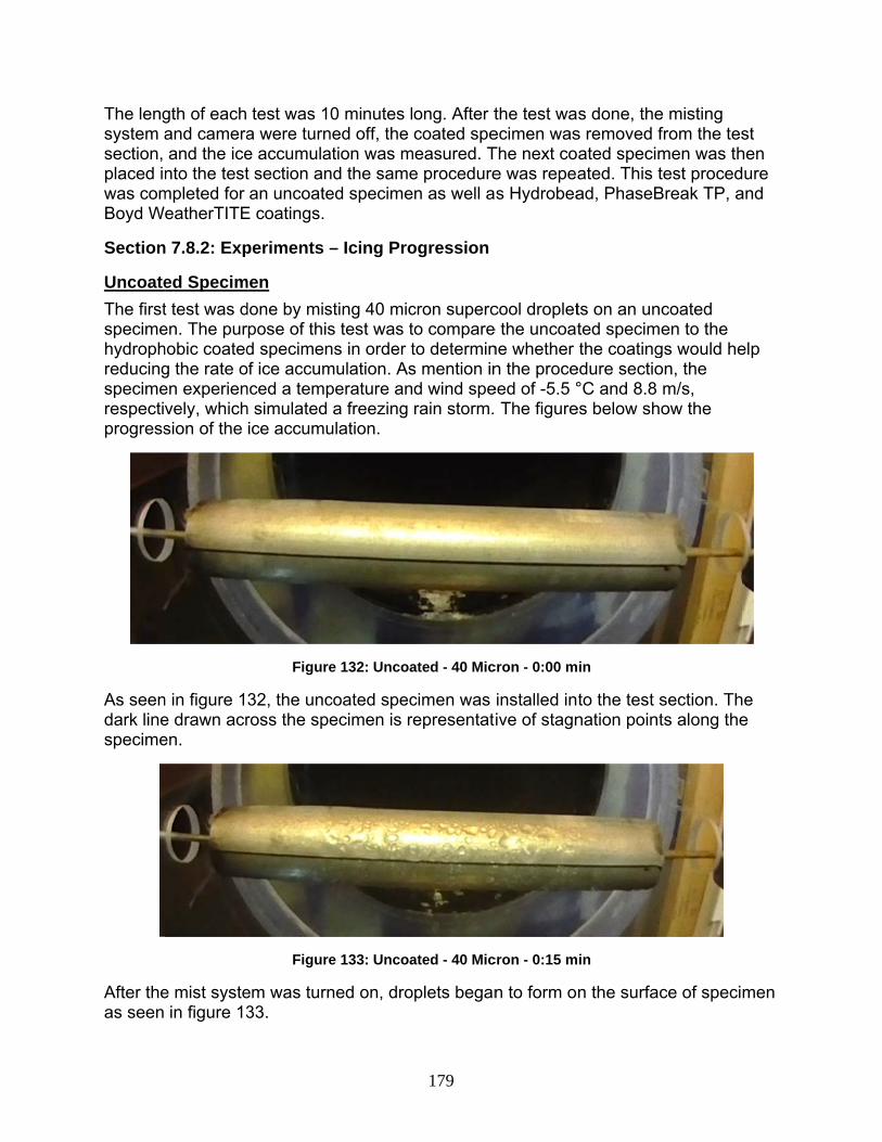
The lengsystem asection, placed inwas comBoyd W

Section

Uncoate

The firstspecimehydrophreducingspecimerespectivprogress

As seendark linespecime

After theas seen

gth of each and cameraand the ice

nto the testmpleted for eatherTITE

n 7.8.2: Exp

ed Specim

t test was den. The purhobic coatedg the rate oen experienvely, whichsion of the

n in figure 1e drawn acren.

e mist systein figure 13

test was 1a were turne accumulat section anan uncoate

E coatings.

periments –

men

done by mispose of thisd specimen

of ice accumnced a temph simulated ice accumu

Figure

32, the uncross the spe

Figure

em was turn33.

0 minutes lned off, the ation was mnd the sameed specime

– Icing Pro

sting 40 mics test was tns in order tmulation. Asperature ana freezing

ulation.

e 132: Uncoa

coated spececimen is r

e 133: Uncoa

ned on, dro

179

ong. After tcoated spe

measured. Te procedure

en as well a

ogression

cron supercto compareto determins mention ind wind sperain storm.

ated - 40 Mic

cimen was representat

ated - 40 Mic

oplets began

the test waecimen wasThe next coe was repeas Hydrobea

cool droplete the uncoatne whether n the proceeed of -5.5 ° The figure

cron - 0:00 m

installed inive of stagn

cron - 0:15 m

n to form o

s done, thes removed fated specimated. This tad, PhaseB

ts on an unted specimthe coating

edure sectio°C and 8.8

es below sh

in

to the test snation point

in

n the surfac

e misting from the tesmen was thtest proced

Break TP, a

coated en to the

gs would heon, the m/s, ow the

section. Thts along the

ce of speci

st hen ure

and

elp

e e

men

As seenwhile wa

As time on the to

n in figure 1ater puddle

passed, theop and bott

Figure

34, dropletsd along the

Figure

e puddle altom of the s

Figure

W

e 134: Uncoa

s were puse stagnation

e 135: Uncoa

ong the staspecimen w

e 136: Uncoa

Water Pu

Water Dropl

Froze

Froze

180

ated - 40 Mic

hed to the tn line.

ated - 40 Mic

agnation linwere still in

ated - 40 Micr

Wate

uddle

ets

en Puddle

en Puddle

cron - 0:30 m

top and bot

cron - 0:45 m

e begin to fliquid form.

ron – 1:00 m

er Droplets

Water Pud

in

ttom of the

in

freeze whil.

min

s

ddle

specimen

e the drople

ets

The frozwater drFigures

The ice The pudwhat haon the b

zen puddle roplets on t136 and 13

continued tddles formeppened at t

bottom of th

Figure

continued the top and 37.

Figure

to accumulad on the tothe stagnate specimen

Figure

e 137: Uncoa

to accumulabottom of t

e 138: Uncoa

ate uniformp and bottotion line. Hon.

e 139: Uncoa

Froz

Wa

Icicle

181

ated - 40 Micr

ate uniformthe specime

ated - 40 Micr

mly on the fiom of the spowever, the

ated - 40 Micr

zen Puddle

ater Drople

es

ron – 1:30 m

mly along then began to

ron – 2:00 m

rst layer of pecimen beere was still

ron – 4:00 m

e

Water Pu

ets

Frozen P

min

e stagnatioo puddle as

min

ice at the segan to freel water drop

min

uddle

uddle

on line whiles shown in

stagnation leze similarlplets formin

e the

line. y to

ng

Figure 1continueicicles d

DropletsaccumuFigures length o

39 shows ted increasinue to the g

s of water hlation. This140 and 14f icicles inc

that the whng as time pravity.

Figure

Figure

had frozen os pattern st41. The thiccreased as w

Figure

ole specimpassed. Th

e 140: Uncoa

e 141: Uncoa

on the earliearted from

ckness of icwell.

e 142: Uncoat

Icic

Ic

182

en was cove ice at bot

ated - 40 Micr

ated - 40 Micr

er layer of uthe right sid

ce accumula

ted - 40 Micr

les

Uneven

cicles

Une

vered with ittom of the

ron – 6:00 m

ron – 8:00 m

uniform icede of the spation contin

ron – 10:00 m

n Surface

even Surfac

ice and the specimen

min

min

e, thus, causpecimen, anued to incr

min

ce

accumulatstarts form

sing uneves see in rease and t

tion ing

n ice

the

Almost 5particulabecame

At the cothickest was plactime, the

The uncprocedushowed measuresize noz

50% of the arly the righ very long b

ompletion opart of the

ced in roome ice shed a

coated specure as abov

ice accretioed to be apzzles.

surface of ht side as seby the end

Figure

of the test, tice was me

m temperatuas one big s

Figure 144:

cimen then e. The dropon the surfaproximately

the specimeen in Figuof the test.

143: Uncoat

the specimeeasured to ure (approxsheet as se

: None Coati

was testedplet sizes oace of the sy 5.5 and 5

183

en is coverre 142. Als

ted - 40 Micr

en was rembe approxi

ximately 21 een in Figur

ng - 40 Micro

d with two of the nozzlespecimen. T

5 mm, respe

red with an so, several

ron – After Te

moved frommately 6.5 °C) and lef

re 144.

on – Shed Ic

other nozzlees were 42 The thickesectively, for

uneven suicicles were

est

m the test semm. The sft to shed. A

e Sheet

e sizes usinand 50 mic

st part of thr 42 and 50

urface of icee present a

ection. The specimen thAfter some

ng the samecron. Both te ice was micron dro

e, and

hen

e tests

oplet

Hydrob

The firsthydrophsprayedminutes

The figucoating t

As seensection. represen

ead

t coating teshobic coatin on the entas instruct

ures below itest experie

n in Figure 1Similar to t

ntative of st

sted was Hng that is cleire surface ted in the m

Figu

illustrate theencing 40 m

Figure

146, the Hythe previoutagnation p

Hydrobead,ear in colorof the spec

manual prior

re 145: Hydr

e progressimicron supe

146: Hydrob

ydrobead-cos test, the d

points along

184

which camr as seen incimen. The r to installat

robead-Coate

ion of the icercool wate

bead – 40 Mic

oated specdark line dr

g the specim

e in a sprayn Figure 145

specimen tion in the t

ed Specimen

ce accumuler droplet si

cron – 0:00 m

imen was irawn acrossmen.

y can. This5. The coatwas allowetest section

n

lation for Hyize.

min

nstalled ints the specim

s is a ting was ed to dry forn.

ydrobead

o the test men is

r 20

The watsystem w

At 30 seThe biggdroplets

ter droplets was turned

econds, the ger droplets remain ne

Figure

began to a on as show

Figure

small wates move to tar the stag

Figure

147: Hydrob

appear on twn in Figur

148: Hydrob

er droplets bhe top and nation line.

149: Hydrob

185

bead – 40 Mic

he surface re 147.

bead – 40 Mic

began to fobottom of t

bead – 40 Mic

Wa

Frozen Dro

cron – 0:15 m

of specime

cron – 0:30 m

orm into bigthe specime

cron – 0:45 m

ater Drople

oplet

min

en once the

min

gger dropleten while th

min

et

e misting

ts or puddlee smaller

es.

As time bigger dbe seen

The frozdroplets

passed, thedroplets on in Figures

zen droplets on top and

Figure

Figure

e smaller dtop and bot149 to 151

Figure

s continuedd bottom of

150: Hydrob

151: Hydrob

roplets alonttom of the .

152: Hydrob

d to accumuthe specim

Frozen Dr

186

bead – 40 Mic

bead – 40 Mic

ng the stagspecimen w

bead – 40 Mic

ulate along men began t

Water

Fro

Wat

Frozen Dr

roplet

Frozen D

cron – 1:00 m

cron – 1:30 m

gnation line were still in

cron – 2:00 m

the stagnato freeze.

r Droplet

ozen Drople

ter Droplet

roplet

Droplet

min

min

began to frn a liquid sta

min

ation line wh

et

t

reeze whileate, which c

hile the wat

e the can

ter

Figure 1causing the grav

More waexperien

53 shows tan uneven

vity.

ater dropletncing ice ac

Figure

that most on ice accum

Figure

Figure

ts froze on tccretion as

153: Hydrob

of the specimmulation. Th

154: Hydrob

155: Hydrob

the previouseen in Fig

187

bead – 40 Mic

men’s surfae ice at bot

bead – 40 Mic

bead – 40 Mic

us layer of icgure 154 an

I

cron – 4:00 m

ace is covettom started

cron – 6:00 m

cron – 8:00 m

ce, thus, thnd 155.

Icicles

min

red with frod forming ic

min

min

he specimen

ozen droplecicles due t

n was

ets o

At the enan unevoriented

Similar ttest wasmm, resplacing i

nd of the exven ice layeddownstream

to the previs completedspectively. Tit in room te

Figure 1

xperiment, r and the icm.

Figure 1

ous test, thd. The thickThe ice sheemperature

156: Hydrobe

the surfacecicles locate

157: Hydrobe

he specimenkest part of eet, shown e for a perio

188

ead – 40 Mic

e of the speed at the bo

ead – 40 Mic

n was remothe ice wasin Figure 15

od of time.

cron – 10:00

ecimen wasottom have

cron – After T

oved from ts measured58, shed fro

min

s completely become lo

Test

the test secd to be appom the spe

y covered bong and

ction once troximately

ecimen whe

by

he 10

en

The Hydsame prBoth tesice was droplet s

PhaseB

The nexcolor as parts webetweenspecimewas folloPhaseB

The PhaFigure 1stagnati

drobead-corocedure. Tsts showed measured size nozzle

Break TP

xt coating teseen in Fig

ere applied n coats as ien was instaowed. The freak TP co

aseBreak T59. Once aon points a

Figure 158

ated specimThe droplet

ice accretioto be appros.

ested was Pgure 159. Ton a specinstructed inalled in the figures beloating exper

Figure 15

TP-coated sagain, the dalong the sp

8: Hydrobead

men was thsizes of theon on the soximately 6

PhaseBreakThis coatingmen using n the manutest sectio

ow portrayriencing 40

59: PhaseBre

specimen wdark line drapecimen.

189

d – 40 Micron

hen tested we nozzles wsurface of th6.5 mm, res

k TP, a supg consisted a foam brual. After then and the pthe progresmicron sup

eak TP – 40 M

was installedawn across

n – Shed Ice

with two othwere 42 andhe specimespectively, f

perhydrophoof 2 parts;

ush and were coating wprocedure dssion of thepercool wat

Micron – 0:00

d into the tes the specim

Sheet

her nozzle sd 50 micronen. The thicfor both 42

obic coatinga primer an

re given timwas fully curdescribed ine ice accumter droplets

0 min

est section men is repre

sizes usingn, respectivckest part ofand 50 mic

g with greynd TP. Both

me to cure red, the n section 6.

mulation for s.

as seen in esentative o

the ely. f the

cron

y h

.3

of

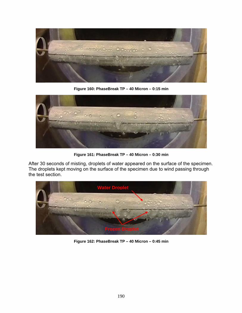
After 30 The dropthe test

seconds oplets kept msection.

Figure 16

Figure 16

f misting, dmoving on t

Figure 16

60: PhaseBre

61: PhaseBre

droplets of wthe surface

62: PhaseBre

Froz

Water D

190

eak TP – 40 M

eak TP – 40 M

water appea of the spec

eak TP – 40 M

zen Drople

Droplet

Micron – 0:15

Micron – 0:30

ared on thecimen due

Micron – 0:45

et

5 min

0 min

e surface ofto wind pas

5 min

f the specimssing throu

men. gh

As time dropletsseen in

The frozdropletsdroplets

passed, the on the top Figures 162

zen droplets on the bot of water st

Figure 16

e water droand bottom

2 and 163.

Figure 16

Figure

s continuedtom of the still appear o

Fr

63: PhaseBre

oplets alongm of the spe

64: PhaseBre

165: PhaseB

d to accumuspecimen bon the top o

Froz

Water

Water D

rozen Drop

Water D

191

eak TP – 40 M

g the stagnaecimen wer

eak TP – 40 M

Break TP – 40

ulate along began to freof the speci

zen Drople

Droplet

I

Droplet

plet

Icicle

Droplet

Micron – 1:00

ation line bere still in a l

Micron – 1:30

0 Micron – 2

the stagnaeeze, creatmen.

et

cicles

es

Frozen

0 min

egan to freliquid state

0 min

2:00

ation line whing icicles.

Droplet

eze while t, which can

hile the watHowever,

he n be

ter

While mthe wate

more ice accer droplets o

Figure

Figure

cumulated aon top bega

Figure

166: PhaseB

167: PhaseB

along the stan to freeze

168: PhaseB

192

Break TP – 40

Break TP – 40

tagnation lie; this can b

Break TP – 40

Frozen Dr

Frozen Dro

0 Micron – 4

0 Micron – 6

ne and the be seen in

0 Micron – 8

roplets

oplets

4:00

6:00

bottom of tFigures 16

8:00

the specim6 and 167.

en,

More drothicknesspecimethe specreally lon

The spethickest melted troom tem

oplets of wass of ice accen continuecimen is cong and orie

ecimen wasof the ice w

to a thin andmperature.

Figure 1

ater froze ocumulation d to increasmpletely co

ented down

Figure 170

removed fwas measud small she

169: PhaseB

on the initiaand the lense as time overed by astream.

0: PhaseBre

from the tesred to be a

eet, shown

193

Break TP – 40

l layer of icngth of iciclpassed. By

an uneven i

ak TP – 40 M

st section approximatein Figure 1

0 Micron – 10

ce as time eles located y the end ofce layer an

Micron – Afte

fter the tesely 10 mm, 71, and she

0:00

elapsed. Boalong the b

f the test, thnd the icicle

er Test

t was comprespectiveled from the

oth the bottom of thhe surface es became

pleted. The ly. The ice e specimen

he of

at

The Phausing threspectivthickest for 42 an

Boyd W

The lastIncorporThere wpart A, Bbrush. Itfully cureprogresswater dr

The WeFigure 1points a

aseBreak Te same provely. Both tpart of the nd 50 micro

WeatherTIT

t coating tesrated and is

were three pB and C. Tht was then ged, the spesion of the roplets.

atherTITE-72. The dalong the sp

Figure 171: P

TP-coated socedure. Thtests showeice was me

on droplet s

E

sted was prs their Weaparts to this he three pagiven time t

ecimen wasice accumu

Figure 1

coated speark line drawpecimen.

PhaseBreak

specimen whe droplet sed ice accreeasured to size nozzels

rovided by atherTITE co

coating, earts were mito cure as i

s installed inulation for W

172: Weather

ecimen waswn across t

194

TP – 40 Micr

was then tessizes of the etion on thebe approxis.

Boyd Coatioating. It isach part caixed and apnstructed in

n the test seWeatherTIT

rTITE – 40 M

s installed inthe specime

ron – Shed Ic

sted with twnozzles ar

e surface omately 6.5

ing Resears a white suame in a seppplied on a n the manuection. The

TE experien

icron – 0:00

nto the test en is repres

ce Sheet

wo other nozre 42 and 5f the specimand 5 mm,

rch Companuperhydrophparated conspecimen

ual. After the figures bencing 40 mi

min

section as sentative of

zzle sizes 0 micron, men. The , respective

ny, hobic coatinntainer labeusing a foae coating wlow show thcron superc

shown in f stagnation

ely,

ng. eled am was he cool

n

After 15 as seen while wa

As time on top aand 175

seconds oin Figure 1

ater puddle

passed, theand bottom 5.

Figure 1

f misting, d173. The drd along the

Figure 1

Figure 1

e puddle alof the spec

173: Weather

droplets of wroplets weree stagnation

174: Weather

175: Weather

ong the stacimen were

W

195

rTITE – 40 M

water appeae pushed ton line.

rTITE – 40 M

rTITE – 40 M

agnation lin still in a liq

Water

Froz

ater Drople

Froze

icron – 0:15

ared on theo the top an

icron – 0:30

icron – 0:45

e began toquid form as

Water D

r Puddle

Water

zen Puddle

ets

en Puddle

min

e surface ofnd bottom o

min

min

freeze whis shown in

Droplet

Droplets

e

f the specimof the speci

ile the dropFigures 17

men men

plets 74

After 1:3while thedroplets

30 minutes,e water dro or puddles

Figure 1

Figure 1

the ice conoplets on tos as shown

Figure 1

176: Weather

177: Weather

ntinued to ap and bottoin Figures

178: Weather

Water D

196

rTITE – 40 M

rTITE – 40 M

accumulateom of the sp176 and 17

rTITE – 40 M

Water Dro

Water

Droplet

icron – 1:00

icron – 1:30

e uniformly pecimen be77.

icron – 2:00

oplets

Ice

r Droplets

Ice

Icicle

Ice Dropl

min

min

along the segan formin

min

let

stagnation lng into bigg

ine er

The ice line. Somicicles st178 and

As time on the tobecome

continue tome of the btarted to bu

d 179.

passed, moop of the sp longer.

Figure 1

o accumulatig water dro

uild up on th

Figure 1

Figure 1

ore layers opecimen fro

W

179: Weather

te uniformlyoplets on tohe bottom o

180: Weather

181: Weather

of ice accreoze as show

Water Dro

I

I

197

rTITE – 40 M

y on top of op of the spof the speci

rTITE – 40 M

rTITE – 40 M

eted at stagwn in Figure

plet Ic

Ice Droplet

Icicle

Ice Droplet

icron – 3:00

the first laypecimen beimen, which

icron – 4:00

icron – 6:00

gnation line.es 180 and

Icicle

ce Droplet

Icicle

t

t

min

yer of ice ategan to freeh can be se

min

min

. All big dro 181. The i

t the stagnaeze and theeen in Figu

oplets of wacicles also

ation e re

ater

The thicBy the edue to wfreeze qThe icicl

ckness of icend of the tewater droplequickly ratheles also bec

Figure 1

Figure 1

e accumulaest, the surets freezinger than sprecome long

Figure 1

182: Weather

83: WeatherT

ation continrface of the g in a previoeading out and oriente

84: WeatherT

Uneven

Uneven

198

rTITE – 40 M

TITE – 40 Mi

nued increaspecimen

ous layer. Ocreate an u

ed downstre

TITE – 40 Mic

Ice Surfac

n Ice Surfac

icron – 8:00

cron – 10:00

asing and sois covered Otherwise, uneven surfeam.

cron – After

ce

ce

min

0 min

o did the leby an unevthe water dface for the

Test

ngth of icicven ice layedroplets thae ice accret

les. er at ion.

After theice accreto be apthe spec

Section

After pecompare

Ta

D

The resuspecimeaccumuduring thfreezes,formed ewater teaccumuthat smaduring thWeather

e test, the setion on the

pproximatelycimen while

n 7.8.3: Res

rforming sue the result

able 42: App

Coaroplet Size

40 micron

42 micron

50 micron

ult show thaen. It is notilation. Thishe tests cau it becomesevenly on thnds to slidelation on thaller droplethe coating erTITE coati

specimen we specimeny 8 mm, rese placing it a

Figure 185:

sult Summ

uperhydrophof each co

roximated ic

ating No

n 6.5

n 5.5

n 5.0

at none of tceable that is due to icusing an uns a thicker he surface e off the suhe speciment sizes causexperimentng. This co

was removen after the tespectively. at room tem

: WeatherTIT

ery of Icin

hobic coatioating and d

ce thickness

one Hy

5 mm 1

5 mm 6

0 mm 6

the coatingst the coatedce droplets neven surfalayer of iceof the uncorface, insten. In additises higher ts. The onlyould be due

199

d from the est. The thiThe ice she

mperature.

TE – 40 Micro

g Tunnel C

ng tests, thdroplet size

comparison

ydrobead

0.0 mm

6.5 mm

6.5 mm

s can preved specimenfreezing qu

ace which c on the surf

oated speciead of gettinon, the resice accumu

y coating the to a differe

test sectionickest part oeet, shown

on – Shed Ice

Coating Te

he table beloe.

n of coatings

PhaseBreak

10.0 mm

6.5 mm

5.5 mm

ent the ice fns tend to huickly rathecan trap morface. On thimen. Due tng trapped.ults of the eulation. Thishat does noent chemica

n. Figure 18of the ice w in Figure 1

e Sheet

ests

ow was gen

s and droplet

k TP Wea

m 8

9

9

from accumave higher

er than spreore water. Ohe other hanto the unifo This causeexperiments is true fort have this al makeup

84 shows thwas measur185, shed fr

nerated to

t sizes

atherTITE

8.0 mm

9.5 mm

9.5 mm

mulating onice

eading out Once the wand, the ice

orm surfacees lower icets also showr most casetrend is theof the coati

he red rom

the

ater

e, the e w es e ing.

200

Section 7.9: Field Experiment Trips

On February 16 and February 20, it was expected of temperatures to go down to the freezing point at Toledo and hence a trip was set up to expose the sensors to a possible icing environment for a more practical test before actual installation. The leaf wetness sensor, ice detector and stay thermistors were used in this field test.

The team from University of Toledo set up stay sheath specimens and exposed them to freezing temperatures. A garden hose sprinkler and Windex bottles were used to simulate rain.

Table 43: Event History (February 16, 2013)

Time Event February 15, 5 – 6 pm Set up ice detector, leaf wetness sensor, sunshine sensor, and

thermistors. Set up CR1000 white boxes.

February 16, 4 am Programmed CR1000s. UT team set up their spraying equipment.

February 16, 4:58 am Started collecting data. February 16, 5 – 6:45 am Water sprayed at random intervals.

Photos captured and results noted. February 16, 6:45 – 8:30 am

Sensors observed, photos taken. Left site at 8:30 am.

February 16, 8:30 – 4:10 pm

Data collected without physical observation. Started packing at 4 pm.

February 16, 4:40 pm Left site for UC.

The UCII team reached Toledo on February 15th evening and set up the sensors and the data acquisition system for the next morning. The team from University of Toledo had already set up a specimen stay sheath identical to those on the bridge on a concrete pad.

Geokon thermistors, same model as those already installed on the VGCS stays were clamped on the stay sheath. Similarly the leaf wetness sensor was also zip-tied on top of the specimen. The ice detector was set up right beside the specimen stay to be exposed to similar simulated weather conditions.

The photos below show the initial set up of the sensors on the experiment pad at Toledo, just a few miles away from the Veteran’s Glass City Skyway bridge (photo credits – Jason Kumpf, University of Cincinnati Infrastructure Institute).

FigureDiffer

FigureRight

e 186: Stay Srent Angles a

e 189: Ice De Beside Stay

Specimens aand Orientati

etector Placey

at ions

Fi

ed Figtied

gure 187: DaS

gure 190: Stad on Sheath

201

ata-logging SSetup

ay Thermisto

System F

ors Zip- FiTa

Figure 188: S

gure 191: Leaped on top

Sunshine Se

eaf Wetness of Specimen

ensor Setup

Sensor n

The diffeaccurateFebruary

F

erent sensoely on its pry 16.

Figure 192: Ic

ors came uprobe. The fo

ce Detector a

p with intereollowing ph

at Various Ti

202

esting resuotos explai

imes Throug

ults. The icein its condit

ghout the Feb

e detector mtion at diffe

bruary 16 Ex

measured icrent times o

xperiment

ce on

Figur

It was obup. Thiswhich wthe 0872heating

As the sbefore inrecorded

re 193: Leaf W

bserved tha was becau

were below f2f1 probe. Isyscle was

stored watenstantaneod by the the

Wetness Sen

at with eachuse the storfreezing. ShInitially the s triggered e

r was warmusly freezinermistor ros

nsor at Vario

h spraying ered water tehortly after deicing threearly. Later

mer, most ong. The sunse, and the

203

us Times Th

event, the temperatureeach sprayeshold wasr it was repr

f it drained/n came out

accumulat

hroughout th

the temperae was aboveying, the was kept low arogrammed

/trickled dowat 7:28 am

ted ice start

e February 1

ature of thee the air/staater froze oat 0.02 inchd to 0.15 inc

wn the ice m, the tempe

ted melting

16 Experimen

e sheath rosay tempera

on the stay aes of ice, sches.

detector prerature .

nt

se ature and

so

robe

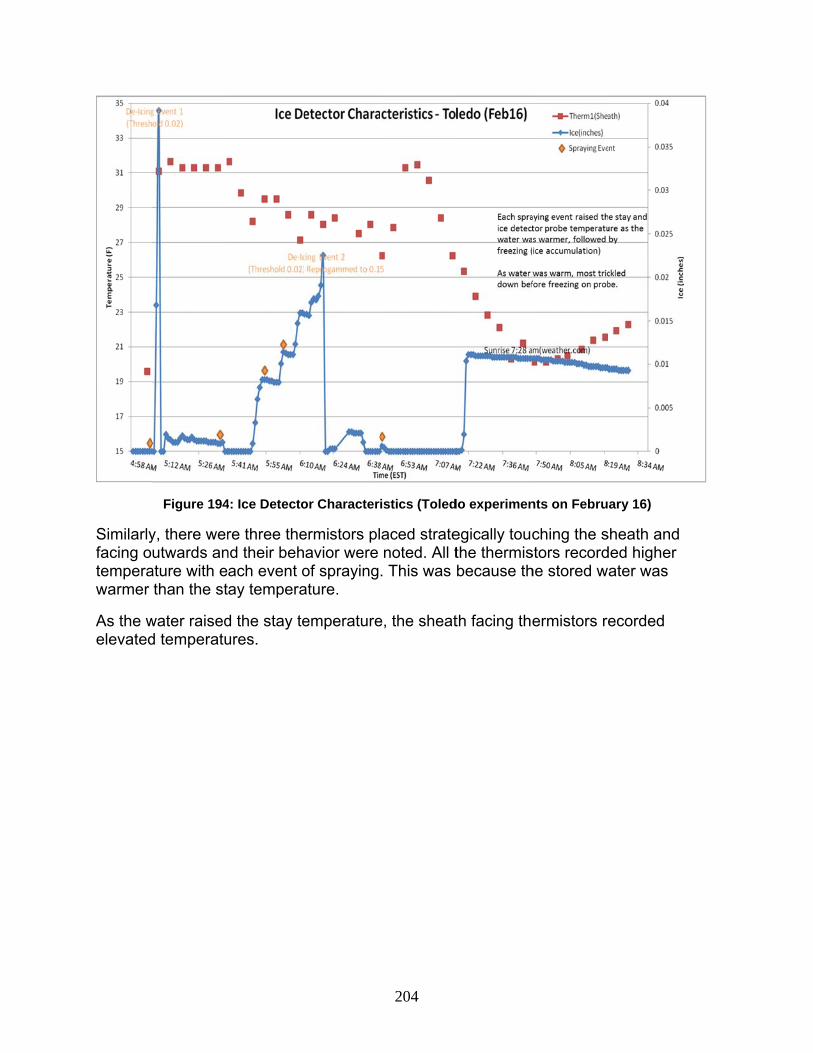
Similarlyfacing otemperawarmer

As the welevated

Figure 194

y, there werutwards an

ature with ethan the st

water raisedd temperatu

4: Ice Detecto

re three thend their behach event oay tempera

d the stay teures.

or Character

ermistors plavior were of sprayingature.

emperature

204

istics (Toled

aced stratenoted. All t. This was

e, the sheat

do experimen

egically toucthe thermisbecause th

th facing the

nts on Febru

ching the sstors recordhe stored w

ermistors re

ary 16)

sheath and ded higher ater was

ecorded

Figure

Fi

e 195: Charac

gure 196: Le

cteristics of

eaf Wetness

205

stay thermis

Sensor ice m

stors (Toledo

melting chara

o, February 1

acteristics

16)

206

During the spraying experiments, water froze on the leaf wetness sensor as well. As a result there was a constant dielectric of about 310 mV when a layer of ice was on its surface.

Later, with sunrise, the characteristics of the leaf wetness sensor were compared to that of the radiation results obtained from sunshine sensor. It could be seen that with each peak (stronger sunshine), the dielectric also showed higher peaks due to melting of ice.

A second trip was made to Toledo on February 20th for another set of tests. The day was carefully chosen as the temperature was supposed to go under freezing point and was considered optimum for icing experiments. On February 20 afternoon, a team from UC went to Toldeo and set up the sensors and data acquisition system. The data loggers were programmed, and the spraying equipments were set up. Around 9 pm, the spraying experiments were started.

Table 44: Event History (February 20-21, 2013)

Time Event February 20, 7:30 pm Set up ice detector, leaf wetness sensor, sunshine sensor and thermistors.

Setup CR1000 & white boxes. February 20, 8:30 – 9:00 pm

Programmed CR1000s. UT team set up their spraying equipment.

February 20, 9:10 pm Started collecting data. Spraying started at 9:13 pm. Water direction changed at 9:19 pm.

February 20, 10:20 pm Left site. UT team stopped hose around 11:00 pm. February 21, 4:00 am Back to site, more photos taken. Ice detector de-iced. February 21, 5:37 – 5:50 am

Ice detector programmed and deployed. Leaf sensor experiment using bug spray.

February 21, 6:03 am Spraying began again. Close observation done to check icing/de-icing characteristics of ice detector. Spraying stopped at 6:34 am.

February 21, 7:12 – 8:40 am

Ice detector disconnected. Other sensors disconnected by 8:40 am as shedding chances were low due to sky cover.

These pFebruaryInstitute

These p

Figur

photos belowy 20 – 21(p)

photos dem

re 197: LWS-

Figure 199:

w are a goophoto credit

onstrate the

-LS with Diff

Ice Detector

od exhibit ots – Jason K

e spraying

ferent Slants

r Setup

207

of the icing eKumpf, Uni

experiment

Figu

experimentiversity of C

ts:

ure 198: Top

Figure 200

ts setup at Cincinnati In

& Side Therm

: First Spray

Toledo on nfrastructur

mistors Setu

y Shower

re

up

Figure 20& leaf sen

Figure 20right duri

Quite simstrategicthe thermbecause

As the welevated

01: Garden Hnsors

02: Ice Detecing deicing)

milar to Febcally touchinmistors rece the stored

water raisedd temperatu

Hose mount o

ctor at Variou

bruary 16thng the sheaorded highe

d water was

d the stay teures.

on ladder (lef

us Times dur

h experimenath and facer temperas warmer th

emperature

208

ft) & hand he

ring Experim

nts there weing outwardture with ea

han the stay

e, the sheat

eld (right) fo

ment (Left and

ere three thds and theiach event oy temperatu

th facing the

r experiment

d Middle dur

hermistors pr behavior wof spraying.ure.

ermistors re

t on ice dete

ring ice accre

placed were noted. This was

ecorded

ector

etion;

d. All

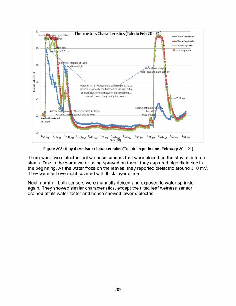
F

There wslants. Dthe begiThey we

Next moagain. Tdrained

Figure 203: S

were two dieDue to the wnning. As t

ere left over

orning, bothThey showe

off its wate

Stay thermist

electric leaf warm waterhe water frornight cove

h sensors wed similar cher faster and

tor character

wetness ser being spraoze on the red with thi

were manuaharacteristicd hence sho

209

ristics (Toled

ensors thatayed on theleaves, theck layer of

ally deiced acs, except towed lower

do experime

t were placeem, they caey reported ice.

and exposethe tilted ler dielectric.

nts February

ed on the saptured high

dielectric a

ed to water eaf wetness

y 20 – 21)

stay at diffeh dielectric around 310

sprinkler s sensor

rent in mV.

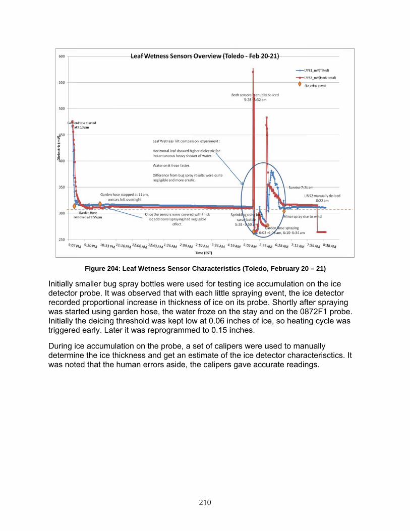
Initially sdetectorrecordedwas starInitially ttriggered

During icdeterminwas note

Figure 204

smaller bugr probe. It wd proportionrted using gthe deicing d early. Lat

ce accumune the ice thed that the

4: Leaf Wetn

g spray bottwas observenal increasegarden hosthreshold w

ter it was re

lation on thhickness anhuman erro

ness Sensor

tles were used that withe in thicknee, the watewas kept loeprogramme

he probe, a nd get an eors aside, t

210

Characterist

sed for testh each little ess of ice oer froze on tw at 0.06 ined to 0.15 i

set of calipestimate of tthe calipers

tics (Toledo,

ting ice accspraying en its probe.the stay annches of iceinches.

pers were uthe ice dete

s gave accu

February 20

cumulation oevent, the ic. Shortly aftd on the 08e, so heatin

used to manector charaurate readin

0 – 21)

on the ice ce detector ter spraying872F1 probng cycle wa

nually acterisctics. ngs.

g be. as

It

Section

The expcoupled functioninitial bethe field consider

Outdoorcalibratio

The testwork revVGCS.

Figur

n 7.10: Con

periments owith the lite

ed as desirehavior in se

station andred at this t

rs experimeon of a new

Geokon Th

LWS-L Dieclassificatio

Sunshine approximat

Goodrich Ic

ts on the coveled there

re 205: Ice D

nclusions

n the sheaterature revred and theervice of thd in the labotime - coati

ents have dw sensor su

hermistor 38

electric Leafon as ice, li

Sensor Bte level of c

ce Detector

oating, fluidis no active

etector char

thing specimiew lead toy were recoe sensors ioratory indings, fluids a

ocumenteduite to be de

800-2-2, for

f Wetness ght rain/sno

F5, for decloud cover

r, for detect

s and heatie technolog

211

racteristics (T

mens at the the concluommend fois discusseicated that and heating

d and verifieeployed on

r stay surfa

Sensor, forow, or heav

etecting anr

ting and qu

ing in combgy that is cu

Toledo, Febr

e field statiousion that thor installatiod in chaptenone of theg - are not v

ed the propthe VGCS

ace tempera

r detecting vy snow/rai

nd quantify

uantifying ic

bination witurrently eco

ruary 20 – 21

on and in thhe proposedon. The Inser 8. The exe active conviable at th

per operatio. These inc

atures

water/moisin.

ying solar

ce thickness

h the earlieonomically f

1)

he laboratod sensors

stallation anxperimentsntrol measuis time.

on and clude:

sture with s

radiation

s

er backgroufeasible for

ry

nd s at ures

some

and

und r the

212

The coating tests at the field station and in the laboratory revealed that the coatings studied did not perform the basic ice prevention function desired. Additionally, they did not age gracefully. If they are durable enough to last a winter, they may discolor or become gummy. Therefore because of poor functionality, low durability and likely installation expense, the existing coatings were deemed infeasible.

213

Chapter 8: Deployment of New Sensors and Upgrade of the Dashboard


The existing sensor array on the bridge was not adequate to accurately characterize the local conditions on the bridge or the stays. The gaps in information from those sensors are presented in Table 2. Where suitable commercial sensors were available, they were procured and deployed on the bridge. The performance of the commercial sensors was verified in the laboratory and the field as described in chapters 6 and 7. The thermistors were mounted directly on the stays and their position and installation is described in chapter 6. The other sensors as well as a pan-tilt-zoom video camera were installed along with the weather tower on the bridge. The weather tower was installed in the spring and summer of 2013 so it could be tested and made available for the 2013-2014 icing season. This chapter describes the location and design of the tower, the deployment of the instruments and camera, as well as the upgrade of the dashboard to incorporate the new sensors. Also, an assessment of the upgraded dashboard’s performance during the following winter (2013-2014) and recommendations to minimize false alarms are presented.

Section 8.2: Self Supporting Instrumentation Tower Design

Section 8.2.1: Tower Design

The weather tower to support the sensors and camera was located on the south eastern end of the bridge. It was on placed on the eastern side so that it would not be in the shadow of the stays for the prevalent easterly ice storms. It was located near the RWIS on the south end to simplify connections and was located so that the sensors were above the stays so no ice would fall on them. The arrangement of the sensors on the tower was chosen such that as much as practical they would not fall in each other’s wind, rain or solar shadow assuming the storm came from the east.

A ROHN self-supporting tower was chosen to support the instruments on the VGCS. The design of the tower was in accordance with national standard ANSI/EIA-222-F and ANSI/TIA-222G “Structural Standards for Steel Antenna Towers and Supporting Structures”. . In the Rohn design report, tower elements were analyzed as three dimensional beam models. A beam element is considered as a two node element with three degrees of freedom at each nodes (two translation and one rotation). The performed calculations for the anchorage system are based on the following maximum factored reactions: maximum download reaction of 21.3 kips, maximum uplift reaction of 20.4 kips, total shear reaction of 1.73 kips, and an over turning moment of 25.21 kip-ft.

The Rohn tower is divided into three sections of roughly equal height, which are the 45GSR for the upper and middle sections and the 45GSRH for the lower section. The reason for this is due to the lower section requires stiffer diagonal and horizontal sections. The Rohn design assumed the base of the tower was 120 feet above the ground. The following design criteria was used: 360 degree wind orientation per 30 degree increment, basic wind speed (no ice) = 90 mph, basic wind speed (with ice) = 40

mph, detopograp

The maxrespectivgoverninbe 0.46.accomm

The demsections

The Roh18, 19 athe westthe cond

Section

The AASdesign. and genspecificaResistanloads intformat aSpecific318 werDesign llimit stattensile sbolt, failucalculati2013 an

esign ice thiphy catego

ximum comvely. Whenng tensile c This show

modate futur

mand to caps, show this

hn tower haand 20, typict side, staysditions durin

n 8.2.2: Anc

SHTO StanThis specif

neral tower ation wherence Factor to an ASD f

and comparation did nore used. A tloads were tes. The folstrength of cure of plateions are pre

nd the instru

ckness = 1ry = 1.

mpressive an considerincapacity of 5ws the tower

re instrume

pacity ratioss standard t

as been inscally most os are usualng the mos

chorage Sy

ndard Sign Sfication is thconcerns. H

eas the RohDesign (LRformat. Whred to the reot provide gtypical doubbased on tlowing failuconcrete, b

e washer, aesented in tuments wer

Fig

.0", exposu

nd tensile fng a govern51.7 kips, thr has capacentation.

s, 0.29 for ttower desig

talled on thof the ice aly bare exct likely icing

ystem Des

Support Sphe most appHowever, thhn loads areRFD) formahen possibleequired streguidance inble nut connthe ROHN ure modes wbase plate fand bearing the (Ali, 20re installed

gure 206: Tow

214

ure categor

forces in legning comprehe demandcity well bey

the 45GSRgn is not be

he east sideccumulates

cept for occg event.

sign

pecification propriate behis is an Alle maximumt, thereforee, nominal sengths. Wh designing nection wasreport, whicwere considailure, fatigstrength of

13). The toshortly the

wer Anchora

ry = C, struc

gs are 20.4essive capad to capacityyond the de

H diagonaling pushed

e of the VGCs on the eacasional froz

was used fecause it adlowable Str

m load envee, it was necstrengths a

hen AASHTof the towes chosen ach considerdered for due failure of concrete.

ower was inreafter.

age System

cture classi

4 kips and 1acity of 44.4y ratio was esign loads

and 0.24 fd to its limit.

CS. As shost side of thzen rivulets

for the anchddresses thress Designelopes in a cessary to fare computeTO Standarder, AISC 14s the anchored strengthesign criter

of base platThe anchostalled in th

ification = I

19.6 kips, 4 kips and adetermined

s to

for horizonta.

own on Figuhe stays. Os. This refle

horage syshe mountinn (ASD) Load and formulate thed in an LRd Sign Sup4th, and ACorage systeh and serviria: bolt failute and anchorage desighe spring of

I,

a d to

al

ures On ects

tem g

he RFD port

CI-em. ce ure, hor n f

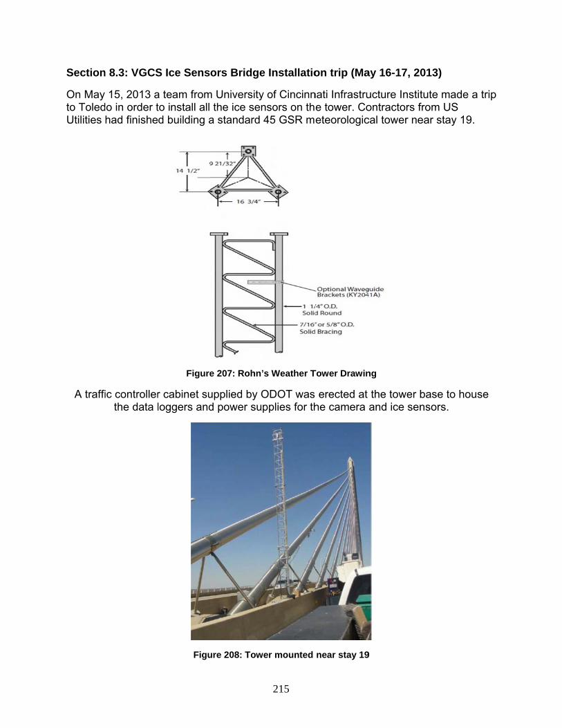
Section

On May to ToledUtilities

A traffi

n 8.3: VGCS

15, 2013 ado in order thad finishe

ic controllerthe data l

S Ice Sens

a team fromto install all d building a

Figure

r cabinet suloggers and

Figu

ors Bridge

m Universitythe ice sen

a standard

e 207: Rohn’

upplied by Od power su

ure 208: Tow

215

e Installatio

y of Cincinnnsors on th45 GSR me

’s Weather T

ODOT was pplies for th

wer mounted

on trip (Ma

nati Infrastrue tower. Coeteorologic

Tower Drawin

erected at he camera

near stay 19

ay 16-17, 20

ucture Institontractors fcal tower ne

ng

the tower band ice sen

9

013)

tute made afrom US ear stay 19.

base to hounsors.

a trip

.

use

On May sensors heights t

a) sb) ric) U

Figu

16, 2013, ton the tow

to support t

et up the dade a bucke

Upgrade the

ure 209: Initia

the URT gawer. Horizon

the sensors

ata loggerset truck ande data acqu

al Plan by UT

athered at Vntal cross-as. The UCII

s inside the mount the

uisition syste

216

T Research T

Veteran’s Garms were fI crew was

tower cabisensors at

em with ne

Team for Tow

Glass City Sfixed on to tdivided into

net, t different e

ew hardware

wer Mounting

Skyway to mthe tower ao three grou

elevations, ae and new

g

mount the t different ups to:

and sampling raate.

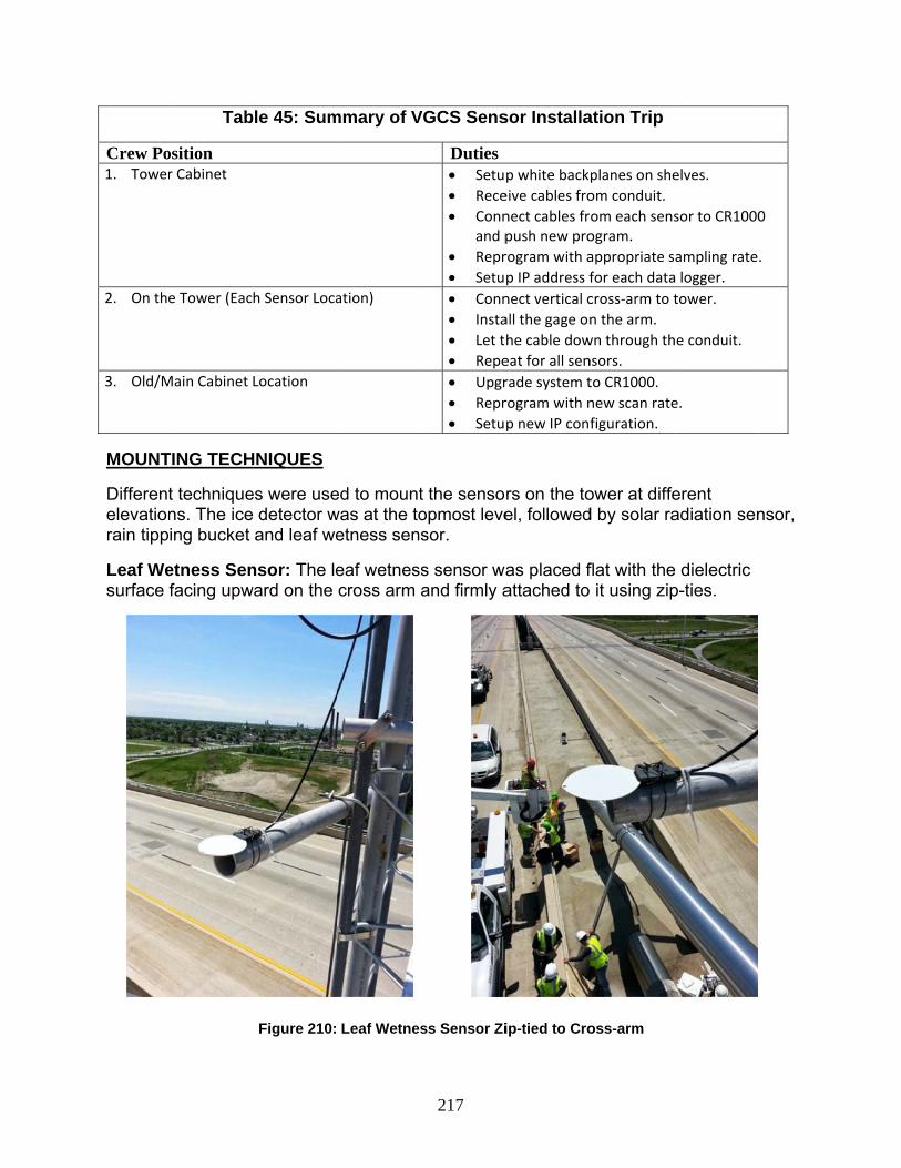
Crew Po1. Tower

2. On th

3. Old/M

MOUNT

Differentelevationrain tipp

Leaf Wesurface

Tab

osition r Cabinet

e Tower (Eac

Main Cabinet

TING TECH

t techniquens. The iceing bucket

etness Senfacing upw

ble 45: Sum

h Sensor Loca

Location

HNIQUES

es were use detector wand leaf we

nsor: The leward on the

Figure 210:

mmary of V

ation)

ed to mountwas at the toetness sens

eaf wetnesscross arm a

Leaf Wetnes

217

VGCS Sens

Duties Setu

Rece

Connand p

Repr

Setu

Conn

Insta

Let t

Repe

Upgr

Repr

Setu

t the sensoopmost levesor.

s sensor waand firmly a

ss Sensor Zi

sor Installa

p white back

eive cables fro

nect cables frpush new pro

rogram with a

p IP address f

nect vertical c

all the gage on

he cable dow

eat for all sen

rade system t

rogram with n

p new IP conf

rs on the toel, followed

as placed fattached to

ip-tied to Cro

ation Trip

planes on she

om conduit.

om each sensogram.

appropriate s

for each data

cross‐arm to t

n the arm.

wn through th

nsors.

to CR1000.

new scan rate

figuration.

ower at diffed by solar ra

flat with the it using zip

oss-arm

elves.

sor to CR1000

ampling rate

a logger.

tower.

he conduit.

e.

erent adiation sen

e dielectric p-ties.

0

.

nsor,

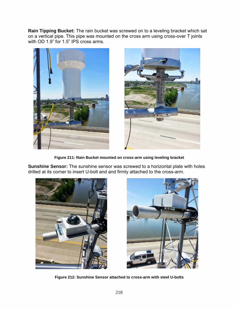
Rain Tipon a verwith OD

Sunshindrilled at

pping Buckrtical pipe. T 1.9” for 1.5

Figure

ne Sensor:t its corner

Figure

ket: The raThis pipe w5” IPS cros

211: Rain Bu

: The sunshto insert U-

212: Sunshi

ain bucket wwas mounte

s arms.

ucket mount

hine sensor-bolt and an

ine Sensor a

218

was screwed on the cro

ted on cross-

r was screwnd firmly at

attached to c

ed on to a leross arm us

-arm using le

wed to a hottached to t

ross-arm wit

eveling bracsing cross-o

eveling brac

orizontal plahe cross-ar

th steel U-bo

cket which over T joints

cket

ate with holerm.

olts

sat s

es

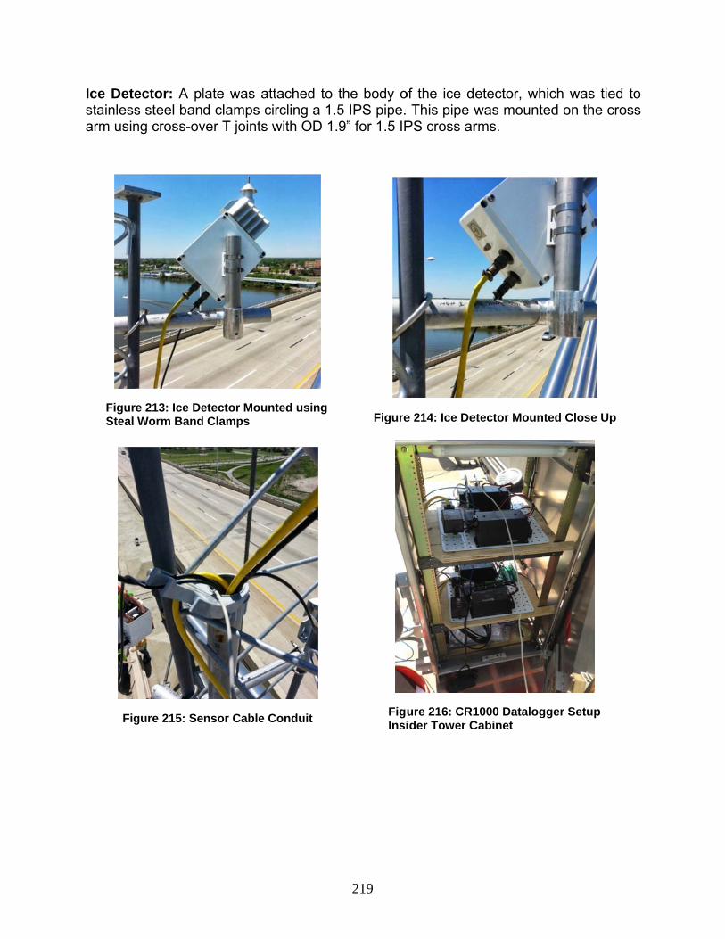
Ice Detestainlessarm usin

FigurSteal

Fig

ector: A pls steel bandng cross-ov

e 213: Ice DeWorm Band

gure 215: Se

late was atd clamps c

ver T joints

etector Moun Clamps

nsor Cable C

ttached to tircling a 1.5with OD 1.9

nted using

Conduit

219

the body o5 IPS pipe. 9” for 1.5 IP

Figure

FiguInsi

of the ice d This pipe wPS cross ar

e 214: Ice De

ure 216: CR1ider Tower C

etector, whwas mountrms.

etector Moun

1000 DatalogCabinet

hich was tieted on the c

nted Close Up

gger Setup

ed to cross

p

Figur

After thestarted c

Section

In chaptdevelopvoters in

Local Sthe eval

IP ConAll theaddres Existin10.102DL1 (IcDL2 (LDL3 (SDL4 (R

All poiNote:

re 217: Close

e sensors wcollecting lo

n 8.4: Chan

ter 5, the auing the accn the algorit

tations: Thuation of th

nfiguratione new data sses provi

ng DL (Stra2.90.236: poce Detecto

Leaf WetneSunshine SRain Bucke

inted to theDL = Data

e up of Weat

were physicocal weathe

nges to the

uthors discucretion algorthm.

here are twhe accumula

n loggers haded by OD

ain Gages,ort 6783

or) – 10.102ess SensorSensor) – 1et) – 10.102

e same exta Logger

her Tower

cally installeer data at th

e Ice Accum

ussed the prithm. The f

o local statation condi

ad to be mDOT IT pers

, Stay Ther

2.90.237: pr) – 10.102.10.102.90.22.90.240: p

ternal IP 1

220

FiguSta

ed, and all fhe bridge st

mulation A

parameters following w

ions havingtions and h

mapped to tsonnel.

rmistors) –

port 6783 .90.238: po239: port 67port 6783

56.63.133.9

ure 218: Comtion Near Sta

firmware cotarting on M

Algorithm

and weathwere added

g five new shence the a

the IP

–

ort 6783 783

93

mpleted Neway 19

onfigurationMay 17, 201

her stations to the prev

sensors thaalgorithm:

w Weather

ns settled, U13.

consideredvious list of

at contribute

UCII

d for

e to

221

Accumulation Determining Stations

1. Accu_Local1: - Stay thermistors and dielectric wetness sensor (leaf wetness sensor)

2. Accu_Local2:- Stay thermistor and rain tipping bucket

3. Accu_Local3 :- Ice detection sensor

The ice detector comprises of a single station alone for simplicity of the algorithm because of its superior reliability and criticality.

Data Update Time: An important factor to consider in the ice determination algorithm is that each of the weather stations have a distinct data update time. In an hour, the RWIS stations update data about 4-6 times an hour, while the METAR stations do it once or twice.

The new local sensors have a sampling rate of 10 minutes so as to read them at a pace that matches those of the RWIS.

Station Individual Weights: According to their importance each existing station had been assigned a weight for its contribution towards triggering an alarm. The closest weather station (RWIS 142-I-280) had a weight of 0.3. Both airports report additional data with high reliability and, hence, also have a weight of 0.3 each. The other three RWIS stations each have a weight of 0.1 because they are farther from the bridge. The new Accu_Local 1, 2, and 3 stations each have a weight of 0.3.

Threshold Weights: Various simulations had been previously done to obtain an appropriate threshold for triggering ice accumulation. The threshold was set at 0.3 so that either of the two METAR airports or the local RWIS station could trigger ice accumulation alert alone. The other three distant RWIS stations can only do the same, when in unison. Each of the new UCII stations included in the proposed algorithm can also trigger this threshold by itself.

Ice Accumulation Algorithm: Sensors in any environment can occasionally misread the actual measurement. The algorithm evaluates all eight weather stations’ (including four RWIS, two METAR, and new UCII stations Accu_Local1, Accu_Local2, Accu_Local3) records for the last hour. Only if a certain percentage of the total records from the last hour meets any of the ice accumulation criteria, then the station has satisfied the icing and is given a Boolean value 1.

However, if this condition is not satisfied by a weather station, the respective station is provided a Boolean value 0. Initially, the percentage of satisfying records is 50% for the new sensors, and 80% for the RWIS / METAR stations. This is then used to find the conditions favorable to ice accumulation by multiplying the Boolean value of each weather station (0 for not met, 1 for met) with the station weight and summing each result.

If the totthat con

In the exHence th

Similarlymodulardecisionand will algorithmto be me

The tablalgorithm

tal weight cditions favo

xisting algohere is a fu

y, three newrity helps upn algorithm work exact

m employedet.

le in the nexm.

Figure 219

calculated, aorable to ici

rithm, thereunction for t

w functions pgrade the for the initiatly the samed with the n

xt page des

9: Flowchart o

as above, ising have be

e have beehe four RW

have beenexisting algal UCII dase as beforenew sensor

scribes the

of existing Ic

222

s greater theen met for

n separate WIS stations

n introducedgorithm withshboard (see, but now itrs which can

modularity

ce Accumula

han a set thr the last ho

functions us, one for th

d for the nehout affecti

een in Chapt is complen also vote

y of the mod

ation Algorith

hreshold (0.our.

used for eahe two MET

ew sensors.ng it; that is

pter 6) remamented by and cause

dified ice ac

hm (Agrawal

.3), we cons

ch station. TAR station

. This kind os, the existiains the sama similar

e the thresh

ccumulation

l, 2011)

sider

ns.

of ing me

hold

n

223

Table 46: Ice Accumulation Station Functions

Ice Accumulation Stations

Function Name Type Measurement Parameters

Exi

stin

g

1. RWIS Web (4 Locations) Precipitation: Rain, Snow Temperature: Air Temp.

2. METAR Web (2 Locations) Precipitation Rain, Snow (various types) Temperature: Air Temp.

Pro

po

sed

3. LocalStation1 Stay Thermistors, Leaf

Wetness Sensor

Precipitation: Dielectric Constant (mV) to wetness check conversion Temperature: Stay Temp.

4. LocalStation2 Stay Thermistors, Rain

Bucket Precipitation: Water collected (inches) Temperature: Stay Temp.

5. LocalStation3 Ice Detection Sensor Ice Presence check directly.

Modular: 3 new independent station functions for ice accumulation criteria

The flowchart below is a good representation of the proposed ice accumulation algorithm. So far we have been using test thresholds for each of the new sensors. The proposed threshold of ice thickness by ice detector is 0.15 after which melting cycle starts. The threshold for leaf wetness sensor is 300 mV and for rain bucket is a rate of 0.1 inches/hr. These thresholds are subject to training in the real world and with more icing events and data analysis, we can settle with a more and more appropriate threshold for each of the new sensors’ icing criterion.

State Trhappensthat persevent coand corr

Different

Once at falling frverificati

Fig

ransitions:s each datasistent ice aonditions peresponding

t states use

C: ‘ClearY1: ‘YellY2: ‘YellY3: ‘YellA: ‘Alert’

Alert, the iom the stayion.

gure 220: Flo

: The detera collection accumulatioersist and toconditions

ed in the Ice

r’–No Ice pow 1’–Icingow 2’–Icingow 3’–Icing’–Ice confir

ce sheddinys. If not, it

owchart for r

mination ofcycle as st

on over houo what extefor transitio

e accumula

resent g possible g likely g highly likemed

g algorithmremains at

224

revised ice a

f possible ictated. Howeurs led to icent requiredon between

ation proces

ely

m gets initiatt this state,

accumulation

ce conditionever, historce sheddingd the develon states.

ss are:

ted, to see unless the

n algorithm

ns (“yes”=1rically it hasg. To determopment of a

if there is pre is a repo

or “no” = 0s been notemine if ice a set of stat

possibility oort after visu

0) ed

tes

of ice ual

225

Section 8.5: Changes to the Ice Shedding Algorithm

The shedding algorithm was revised to include some of the new sensors in addition to the 6 off-bridge stations used before. The new sensors used are reffered to as “Local Stations”.

Local Stations: There are two local stations having two sensor types that contribute to the shedding conditions and hence the algorithm:

1. Fall_Local1 :-Stay Thermistor

2. Fall_Local2 :- Sunshine Sensor

Data Update Time: An important factor to consider in the ice determination algorithm is that each of the weather stations has a distinct data update time. The RWIS stations update data about 4-6 times an hour, while the METAR stations do it once or twice.

The local sensors have a sampling rate of 10 minutes.

Station Individual Weights: According to the importance of each station, they had been assigned weights for their contribution towards triggering an alarm. The closest weather station (RWIS 142-I-280) has, thus a weight of 0.3. Similarly, both the airports report additional data and hence also have a weight of 0.3 each. The other three RWIS stations each have a weight of 0.1. The new Fall_Local 1 and 2 stations based on local icing sensors on the bridge are designed to have a weight of 0.3 in the algorithm.

Threshold Weights: As before, the threshold was set at 0.3 so that either of the two METAR airports or the local RWIS station could trigger ice accumulation alert alone. The other three distant RWIS stations can only do the same, when in unison. Each of the local stations included in the revised algorithm can also trigger this threshold by itself.

Ice Shedding Algorithm: As previously mentioned, sensors in any environment can occasionally misread the actual measurement, thus, each of the eight weather stations’ (including four RWIS, two METAR, and new local stations Fall_Local1, Fall_Local2) records are evaluated for the last hour. Only if certain percentage of the total records from the last hour meets any of the ice shedding criteria, then the station has satisfied the icing criteria as for the last hour and is given a Boolean value of 1.

However, if this condition is not satisfied by a weather station, the respective station is provided a Boolean value 0. The percentage is 50% for the local sensors, and 80% for the RWIS / METAR stations. This is then used to find the conditions favorable to ice shedding by multiplying the Boolean value of each weather station (0 for not met, 1 for met) with the station weight and summing each result.

If the total weight calculated, as above, is greater than a set threshold (0.3), we consider that shedding conditions have been met for the last hour.

In the exstationsMETAR

Similarlof modu

The tablalgorithm

F

Exi

stin

g

1.

2.

Pro

po

sed

3.

4.

xisting algo, hence, thestations.

y, two new ularity helps

le in the nexm.

Figure 2

Function Na

RWIS

METAR

LocalStatio

LocalStatio

Modular:

rithm, thereere is a sep

functions hs upgrade th

xt page des

21: Flowcha

Table 47

ame

W

W

on1 S

on2 S

: 2 new inde

e have beeparate funct

have been he existing

scribes the

rt of existing

: Ice Fall St

Ice She

Type

Web (4 Locat

Web (2 Locat

Stay Thermis

Sunshine Se

ependent sta

226

n separate tion for the

introduced algorithm w

modularity

g Ice Sheddin

tation Funct

edding Chec

tions) T

tions) ST

stors T

ensor S

ation function

functions ufour RWIS

for the newwithout affe

y of the mod

ng Algorithm

tions in alg

ck Stations

Meas

Temperature

Sky cover: ClTemperature

Temperature

Sky cover: So

ns for ice ac

used for ea stations an

w local sensecting it.

dified ice sh

m (Agrawal, 2

gorithm

surement Pa

: Air Temp.

louds/visibili: Air Temp.

: Stay Temp

olar Radiatio

cumulation c

ch of the sind the two

sors. This k

hedding

2011)

arameters

ty.

p.

on (Watts/m2

criteria

ix

kind

2)

The flowfar test tthresholmore ap

Section

In previodiscusse

The mai

1. D2. M3. H4. D5. P

wchart belowthresholds hd is set at 1

ppropriate th

n 8.6: Chan

ous sectioned. This cha

in website h

Dashboard Map (WeathHistory DocumentatPlotting

w is a goodhave been 125 Watt/mhreshold fo

Figure 222: F

nges to the

s of this chapter expla

had severa

her Data by

tion

d representaused for ea

m2. With moor each of th

Flowchart fo

e Dashboar

apter, the dains how the

l tabs:

location)

227

ation of theach of the nre icing evehe new sen

or revised ice

rd

design and e algorithm

e revised icenew sensorents and dansors’ icing

e shedding a

functionalit is impleme

e shedding rs. The solaata analysiscriterion ca

algorithm

ty of the algented for fro

algorithm. ar radiation s, a more aan be set.

gorithm wasont end use

So

nd

s er.

Section

The inpuPython aorder to

The funcweatherdata. Thof weathdeveloponce pe

Upgradethat deteany of th

At the bothe four not repodashboadashboa

Ta

n 8.6.1: Das

uts from thealgorithm wintegrate d

ction of the r measuremhese procesher measured to carry r hour.

e of the dasermines thehe six statio

ottom of theRWIS and

orting data. ard. Pleaseard panel:

abs of ice mon

shboard M

e sensors gwas exhibitedata from an

first part wments of thesses needeements froout the aut

shboard: A e functionalons has not

e main pantwo METAThe main p find below

F

nitoring website

Speedomet

ain Panel

go into a Pyed through tnd manage

was to autome RWIS stated to be abim all the aptomated ev

new modul status of et been repo

el is the tabAR stations.panel also i

w a screen s

Figure 223: D

e

ter dial

Mo

228

ython algorithe dashbo

e connectivi

mate the cotions, airpoding and stppropriate svaluation pro

le has beeneach remoteorting enoug

ble that shoThe greenncludes the

shot of the w

Dashboard M

Ticke

onitor of Monit

thm. The ioard was divity between

ollection, arort METAR aturdy so thasources. Throcess and

n added to e weather sgh data in t

ows the funn symbol ture links to alweb site sh

Main Panel

er for last 48 ho

tor: Weather st

mplementavided into f

n separate s

rchiving andand weatheat we have he softwareput on sche

the dashbostation. It rethe past one

nctional statrns red for ll other pag

howing the m

ours record

tation status

ation of the few parts insystems.

d data mininer tower sea reliable s

e was finallyedule to run

oard algoritheports whene hour.

tus of each each statio

ges of the main

n

ng of nsor set y n

hm n

of on

229

Section 8.6.2: Map (Weather Data by location)

As before, the icing monitor website includes an interactive map of the weather stations. It contains pop-up balloons for each weather station where current sensor readings are shown and historical readings can be plotted on a timeline. The map also provides view of the cameras installed on the bridge. Google Maps API has been used for this application. Google Maps is a free web mapping service provided by Google, which offers street level maps for pedestrians, cars, and public transportation.

The Google map on the dashboard is used as a graphical interface providing the particulars about the various weather sites being monitored for determining the icing conditions at VGCS. It also contains the location of various sites, their past/present weather conditions along with their source links.

Initially, this weather map comprised of the few RWIS, METAR and local stations surrounding the bridge. After successful installation of the various new ice sensors on the bridge, new station have been added to the weather map comprising information about these UCII sensors and newly installed camera.

When thcorrespothem. Th(Metcalfstationsstations represensensors

Figure 224

he map tab onding to thhese are thf Field Airpo. There arenear to the

nts the UCIprovide de

4: Example S

is clicked, he different he two Airpoort. The fou two yellow

e VGCS BriI sensors s

etailed infor

Snapshot of W

the Googlestations. T

orts namelyur red balloow balloons w

dge. Anothstation. In thrmation thro

230

Weather Map

e map openThere are twy KTOL (Toons written written “L” oher green mhe UCII maough a 48 h

p, with Pop-u

ns with sevewo green baoledo Expre

“R” on themon it. These

marker with arker, on clichour plot. H

up for Ice De

eral markeralloons writess Airport) m are the foe are the loc“U” written cking any o

Here are exa

etector

rs tten “A” on and KTDZ

our RWIS cal weatheron it

of the ice amples:

r

Similarlyby clicki

Section

The plotdifferentbe popurange of

Accordinrange. A

Figur

y, the last 4ng the appr

n 8.6.3: New

tting tab hat sections a

ulated with tf the start a

ngly, the daAt present t

re 225: Last

Figure 226:

48 hour plotropriate link

w Sensors

s been upgas illustratedthe differenand end dat

ata for the dhe different

48 hour repo

Last 48 hou

ts for the iceks in the ma

Plotting

graded to ind in the Figt stations/s

te for this p

different sent sections in

231

ort of Solar S

r report of Le

e sensor anarker.

nclude the loures 227 -

sensors it colotting func

nsors can bn the ice mo

Sensor (Glob

eaf Wetness

nd the rain

ocal senso232 below.onsists of. T

ction.

be obtainedonitor plotti

bal Radiation

s Sensor

sensor can

rs. This plo. Each plottThe user ca

d for the desing tab are:

n)

n be obtaine

otting tab hating sectionan select th

sired time :

ed

as n can he

Figure 227: S

Figure 228:

Stay 20 Ther

Stay 8 Therm

232

rmistors plot

mistors plot

t (January 1 –

(January 1 –

– July 1)

– July 1)

Figure

Figure 230:

229: Ice Det

: Leaf Wetne

233

tector plot (J

ss Sensor p

June 1 – July

lot (June 1 –

y 1)

– July 1)

Figure 231

Figure 23

: Rain Tippin

32: Sunshine

234

ng Bucket pl

e Sensor plot

ot (June 1 –

t (June 1 – J

July 1)

uly 1)

235

Section 8.7: Insights Gained from the Operation of the Upgraded Dashboard

Since the installation of the new ice sensors by University of Cincinnati Infrastructure Institute in May 2013, we have been able to obtain data for one season of winter, December 2013 – April 2014. To test the performance of the new sensors before being installed, rigorous testing methods had been implemented in the lab and in the field. Those experiments helped us understand the nature and anticipate the usefulness of the sensors when deployed in the real world. However, to establish ground truth of the actual performance of the sensors, the training data obtained this winter is very important.

This winter had been quite eventful as far as wintry conditions are concerned. We have had multiple occasions where our upgraded dashboard algorithm triggered ice accumulation warnings, mostly at moderate levels of Y1 (level 1 ice accumulation), few Y2 (level 2 ice accumulation) and Y3 (level 3 ice accumulation). There has been no incidence where the dashboard warned ice shedding.

The remote weather sensors from RWIS and METAR stations had helped our ice event determination algorithm the past few winters. However, that data wasn’t short of various issues including time delay, inaccuracy and lack of local supervision. The new sensors – ice detector, leaf wetness sensor, solar radiation sensor, rain tipping bucket and stay thermistor have paved way to a new level of microclimate information at the Veteran’s Glass City Skyway bridge. Each of them has been obtaining different and crucial data for ice accumulation and/or ice shedding event determination.

The stay thermistors had been installed on the bridge in April 2013. However, the other sensors were installed more recently and were exposed to icing conditions on the bridge for the first time this past winter. The collection of ground-truth data will enable calibration of remote-sensing data for the years to come, and aid in the interpretation and analysis of the weather parameters.

The events triggered by the sensors this winter are enumerated in the following table:

236

Table 48: Chronology of winter 2013/2014 icing event triggers Date Highest

Dashboard Status

Stations/Sensors Triggered

12/09/2013 Alert KTOL, ODOT Report 12/11/2013 Y1 Stay Thermistor + Dielectric Sensor

12/12/2013 Y1 Stay Thermistor + Dielectric Sensor

12/13/2013 Y2 RWIS2016, Stay Thermistor + Dielectric Sensor

12/14/2013 Y3 Stay Thermistor + Dielectric Sensor 12/23/2013 Y1 RWIS2016

12/29/2013 Y1 KTDZ, RWIS2016

01/01/2014 Y1 Stay Thermistor + Dielectric Sensor, RWIS2016

01/04/2014 Y1 RWIS2016 01/05/2014 Y2 RWIS2016, Stay Thermistor + Dielectric Sensor,

KTDZ

01/09/2014 Y1 KTDZ

01/10/2014 Y2 Stay Thermistor + Dielectric Sensor, RWS2016

01/17/2014 Y1 RWIS2016

01/20/2014 Y1 Stay Thermistor + Dielectric Sensor, RWIS2016 02/20/2014 Y2 Stay Thermistor + Dielectric Sensor, RWIS2016

03/08/2014 Y1 Stay Thermistor + Dielectric Sensor,RWIS2016,RWIS2013, KTOL, KTDZ

03/12/2014 Y2 KTOL, KTDZ

03/29/2014 Y1 KTDZ 04/03/2014 Y2 Stay Thermistor + Dielectric Sensor, Stay Thermistor

+ Rain Bucket, KTDZ, Ice Detector

04/15/2014 Y1 KTOL, Stay Thermistor + Rain Bucket

*Note: The weight of the station for leaf wetness sensor + stay thermistors was reduced to 0.1 in early January, thus reducing false alarms.

Section 8.7.1: Ice Events (Winter 2013/2014)

Thanks to the polar vortex/jet stream, this winter provided decent opportunities for the icing sensors to be tested out in the real world where there is dust, debris and reduced access to maintenance. There were several days where the temperature was way below freezing temperature, and there was ample precipitation.

We had multiple ice accumulation incidents; however, there were no prominent instances of ice shedding. Some of the significant days are enumerated below:

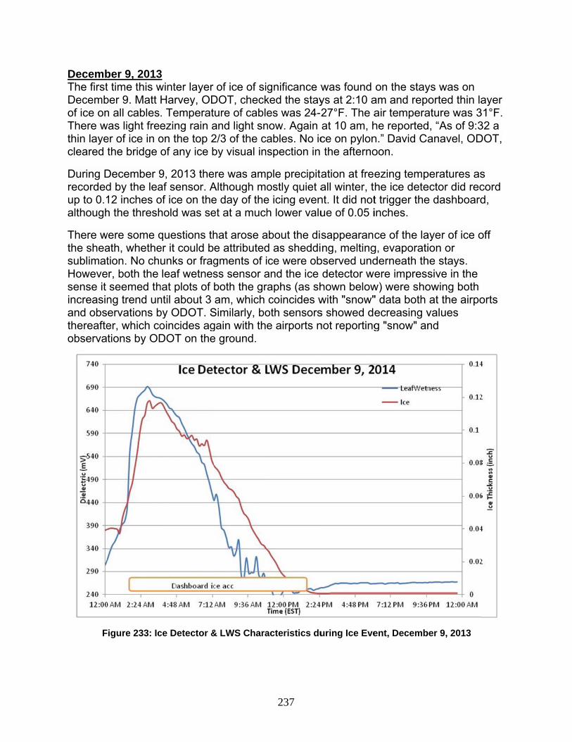
DecembThe firstDecembof ice onThere wthin layecleared

During Drecordedup to 0.1although

There wthe sheasublimatHowevesense it increasinand obsthereafteobserva

F

ber 9, 2013t time this wber 9. Matt n all cables

was light freeer of ice in othe bridge

December 9d by the lea12 inches oh the thresh

were some qath, whethetion. No chu

er, both the seemed th

ng trend unervations ber, which cotions by OD

Figure 233: Ic

3winter layer Harvey, OD. Temperatezing rain aon the top 2of any ice b

9, 2013 theaf sensor. Aof ice on thehold was se

questions ther it could bunks or fragleaf wetnes

hat plots of ntil about 3 by ODOT. Soincides agDOT on the

ce Detector &

of ice of sigDOT, checkure of cableand light sn2/3 of the caby visual ins

re was ampAlthough moe day of theet at a much

hat arose ae attributedgments of iss sensor aboth the graam, which

Similarly, bogain with thee ground.

& LWS Chara

237

gnificance wked the stayes was 24-2

now. Again ables. No icspection in

ple precipitaostly quiet ae icing evenh lower valu

about the disd as sheddice were ob

and the ice aphs (as shcoincides w

oth sensorse airports n

acteristics du

was found ys at 2:10 a27°F. The aat 10 am, hce on pylonthe afterno

ation at freeall winter, tnt. It did notue of 0.05 i

sappearancng, melting

bserved unddetector wehown belowwith "snow"s showed denot reporting

uring Ice Eve

on the stayam and repair temperahe reportedn.” David Caoon.

ezing temphe ice detet trigger theinches.

ce of the lag, evaporatiderneath there impress

w) were sho" data both ecreasing vg "snow" an

ent, Decemb

ys was on orted thin la

ature was 3d, “As of 9:3anavel, OD

peratures asector did rece dashboard

ayer of ice oion or

he stays. sive in the owing both at the airpo

values nd

ber 9, 2013

ayer 31°F. 32 a DOT,

s cord d,

off

orts

238

December 13 & December 14, 2013

The rest of the month of December saw few minor accumulation events. A lot of ice accumulation alerts were triggered between December 13 and December 14, 2013. Initially it was just the local RWIS2016 sensor that reported freezing rain. This was followed by consistent simultaneous reporting of high dielectric and sub-zero temperature by the leaf wetness sensor and the stay thermistors respectively. The dashboard reported level Y3 at 4 pm on December 14. This was a significant cause for concern and called for some visual report, this being among the first events for the new ice sensors. However, Matt Harvey, ODOT reported, “Found no ice, very little snow on cables. Cable temperature at 4:47 am was 19.5-23°F. Pylon temperature was 21°F”.

January 5, 2014

There were just a few sporadic triggers on the 1st of January, but January 5th marked the first true ice event of the year 2014, as there was a lot of ice accumulation warnings from the dashboard on this day. The local RWIS2016 reported freezing rain in the previous evening, which was followed by snow as reported by the Toledo Metcalf Airport. The leaf wetness sensor also triggered higher dielectric. The dashboard stayed at Y2 for three hours.

January 10, 2014

On this day the icing alarm was triggered by the local RWIS2016 station, and the Leaf Wetness Sensor with stay thermistors. Initially freezing rain was reported by RWIS2016 which was followed by snow. The dielectric LWS reported higher dielectric. It was, in fact one of the days when it recorded about 800-900 mV dielectric which usually signifies rainfall. The rain bucket tipped twice in long intervals, and recorded lower precipitation than its threshold (set at 0.05 inches) thus failing to set its flag to true for the ice accumulation trigger. Trace of ice was measured by the ice detector as well, although that didn’t trigger the alarm. According to National Weather Service, there were 0.46 inches of precipitation and 0.6 inches of snow.

February 20, 2014

The dashboard started reporting icing conditions since 1 o’clock in the morning. This was triggered by the local RWIS sensor 582016 which reported freezing rain. At 6 am the status moved to Y2 and continued staying at Y2 for 3 more hours. The RWIS 2016 stopped reporting freezing rain activity and the status came down to Y1 at 9 am. This time both the airports signaled freezing rain conditions. The wetness sensor also reported higher dielectric.

On this dtrigger thnot a casatisfyinInstead,sensor wright on The oute

day the ice he dashboase of misse

ng the cond the ice thic

was zero (itthe device er stay ther

Figure 23

detector mard althouged detectionition of havckness quicts de-icing tprobe natu

rmistors dw

34: VGCS Ici

measured 0.h the thresn as there w

ving enoughckly fell to 0threshold burally. Windwelled unde

239

ing camera v

.06 inches ohold was sewas just thih records in0.01 inchesbeing set at

or bridge vr 32°F long

view before n

of ice, but iet at 0.05 ins one spike

n one hour t. Since the0.15 inche

vibrations mger than oth

noon

interestinglynches. Howe above theto set the ic heat time r

es), sheddinmay be a poher thermist

y, this did nwever, this we threshold,cing flag. recorded by

ng happeneossible cautors possibl

not was , not

y the ed se. ly

March 1

The MarAccordinthe top wthe sideprogresssticking

The airpdashboacovered

April 3,

The dascontinuetemperaand precwetnesssome frewas a st

PersonaDouglasstays abthe stay

Figure 235:

12, 2014

rch 12 ice ang to predicwas expects of the VGsion of timeefficiency a

ports continard alerts. T and hence

2014

shboard reced to registeature stayincipitation cos sensor aneezing raintrong possi

al communis K Nims, Ubout 3 pm as (~1/32') a

Ice Detector

accumulatioctive analysted. Until 2

GCS or PMBe, and the teand the volu

ued to repoThe ice detee were inco

corded its fier no ice. Tg higher thaontinued. Pd the rain t. As a resulbility of rea

cation was University ofand 3:45 pmat 3 pm and

r & Leaf Wet

on event wasis by Dr. N pm, the snB specimenemperatureume of sno

ort cold andector didn’tnclusive as

rst Y1 at 11The RWIS &an the stay

Precipitationipping bucklt, the dash

aching Y3 st

made betwf Toledo, "I

m. He obsed it was gon

240

ness Sensor

as mostly dNims, flecksnow was dryns even thoe dropping aow in the air

d fog which show icing

s well.

1 am and Y& METAR wy temperatun was confirket. The airboard wenttatus.

ween UCII aspoke with

erved a thinne when he

r characteris

driven by fogs of ice and y enough th

ough the winand the snor was gettin

is what hadg. The came

Y2 at 5 pm. weather staure. Temperrmed in unirport at Tolet up to Y2.

and UT resh Dave Kann layer of ice crossed ba

stics on Febr

g in the mothen a slighat it was nnd was steaow slowing ng lesser.

d been triggeras appea

The ice dettions recordrature of thison by bothedo MetcalfIf this conti

earchers. Anavel. He he that did nack over at

ruary 20

orning. ht build up

not sticking ady. With down, both

gering the ared to be s

tector BF5 ded air e stays diph the leaf f also reporinued, there

According tohad checkednot wrap arot 3:45 pm.

on to

h the

snow

ped

rted e

o Dr. d the ound The

241

ice extended about 30 feet up the stays. The ODOT weather service forecast is for the temperature to rise to 40°F by midnight."

Some shedding was observed as well later this day. Shedding was observed. According to Clint Mirto, student, University of Toledo, icing was occurring on VGCS. As large as a five feet piece of ice was reported to fall off around 4 pm.

This was another event of significance as the ice detector triggered the alarm the only time this winter. It recorded 0.16 inches of ice at 11:50 am. The deicing threshold was set at 0.15 inches and the heater melted the ice, but it recorded 0.13 inches of ice again at 1 pm. Interestingly, the ice shed off the probe, but not because the heater went into de-icing cycle this time. The ice detector recorded zero seconds of heating time which means the heater did not get turned on. The shedding of the ice on the probe can possibly be attributed to natural causes like wind or vibrations. The shedding/melting of ice on the stays around 3 pm – 4 pm can be attributed to the rising temperature of the stays above 32°F and little peaks of solar radiation (~120 Watt/m2). This was a good day for observation of the heated rain/snow gage performance. The rain bucket too tipped constantly several times during the heavy showers. According to National Weather Service, there was 1.15 inches of precipitation on April 3rd, 2014.

April 15, 2014

April 15th has been marked as the last day of icing alert recorded this winter season. There were two alerts of Y1. This was also the second time the rain tipping bucket was the cause of an alarm. The rain bucket tipped few times between midnight and 3:20 am. The local airport at Toledo (KTOL) also set the alarm due to snow. The ice detector measured very mild accumulation after midnight. According to National Weather Service, there was 0.13 inches of precipitation on this day.

F

Figure 2

Figure 237: R

36: Ice detec

Rain Tipping

ctor & Leaf w

Bucket & Le

242

wetness Sens

eaf Wetness

sor characte

Sensor char

eristics on Ap

racteristics o

pril 3

on April 3

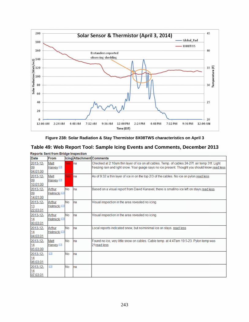
F

Table 4

Figure 238: S

49: Web Re

Solar Radiati

eport Tool:

on & Stay Th

: Sample Ic

243

hermistor 8X

cing Event

X08TWS char

ts and Com

racteristics o

mments, De

on April 3

ecember 2

2013

244

Section 8.7.2: Sensor Performance

All the sensors (remote RWIS/METAR stations as well as the new local sensors) gave us useful information this past winter. There were several instances of ice accumulation alarms and we can say, it has been but a busy winter at the Veteran’s Glass City Skyway bridge. However, in spite of the added sensors, there were cases where we had false alarms, possible missed detections of shedding, as well as loss of data during a large power outage in January 2014. It was observed that the majority of the ice accumulation events were triggered by the leaf wetness sensor and the local RWIS station at VGCS (RWIS2016). A good number of these were false alarms; the RWIS2016 sensor broke down a few times. The RWIS 582016 has had a history with its rain sensor being stuck during freezing rain. This year RWIS 2013 and KTDZ also were down a few times, not providing data seamlessly. Similarly, the local sensors albeit more dependable, were not perfect either.

Dielectric wetness sensor

The dielectric leaf wetness sensor triggered the dashboard many times, some of which were false triggers. This has to do with the threshold being used in the algorithm mostly. As the sensor is sensitive to very low quantity of moisture, raising its threshold in the algorithm or forming a band of freezing conditions(290-310 mV) after high dielectric activity( >400 mV) can help reduce these false alarms. However, it gave us vital triggers on events such as December 14 and February 20th when the ice detector did not measure any ice. Due to its high frequency of false alarms, the weight of the sensor station was lowered from 0.3 to 0.1 in the ice accumulation algorithm in early January following which this problem was resolved. Nevertheless, the current threshold used for the LWS leaf wetness sensor needs to be adjusted apropos to visual inspection and more training data in the future.

Stay Thermistors

The stay thermistors are beyond doubt some of the most crucial sensors on the bridge. This is because the icing algorithm requires temperature data in addition to the precipitation data provided by sensors like leaf wetness sensor and rain tipping bucket. The stay thermistors provided valuable data for the stay temperature throughout the winter. This data was necessary as knowledge of stay temperature is more instrumental for quicker determination of icing events which the remote RWIS/METAR data do not provide. The thermistors placed at different positions and directions gave us appropriate data of temperature of the stays. During melting conditions, it was observed that sheath thermistors got warmer sooner that the outer thermistors due to latent heat required to melt the ice. Here the sensor chosen 7X20TUS is the thermistor directly lying on the sheath while the sensor 7X20TUO is facing more outwards.

Figu

F

ure 239: Leaf

Figure 240: S

f Wetness Se

Stay Thermis

245

ensor charac

tor characte

cteristics win

eristics winte

nter 2013/14

er 2013/14

Rain Tip

The headevoid odevice nfrom dusfilament gage. Thtime to t

The rainwell by i

Figure 24

pping Buck

ated rain/snof regular mneeds to best and debrand melt, s

he tipping btime so that

n bucket alwtself recent

41: Sheath th

ket

ow tipping maintenancee removed dris. Removaso that the bucket insidt it tips accu

ways gave atly on icing

hermistors w

bucket mose and was pduring snowal of the screquivalent

de consists urately with

accurate daevents of A

246

warming fast

stly gave inpossibly dowfall and rereen enableprecipitatioof a hinge

hout getting

ata in the laApril 3rd and

ter than oute

naccurate reown. The preinstalled afes the snowon can be mthat also ne stuck.

ab experimed April 15th,

er (March 4, 2

esults all wrimary screfter snowfalw to reach tmeasured beeds to be

ents, and h 2014.

2014)

inter as it wen of the ll to protectthe heated by the tippin

calibrated

as perform

was

t it

ng from

med

Ice Dete

Althoughhardly reaccumuglides dofeature, sensor pof 0.15 iautomat

Deeper algorithminches omore resthe algothe ice ocauses lmay disameasureBesidessheddin

Fig

ector 0872

h the most ecorded mulation throuown beforewhich is cr

probe shed nches (Febted heating

analysis nem had a casof ice. Sincesearch neerithm appro

on the senslike wind orappear dueement shou measuremg events.

gure 242: Rai

F1

popular cauch accumuugh freezinge freezing orucial to its f

off naturalbruary 20 &.

eeds to be dse of missee automateeds to be doopriately (fosor probe gor vibration. e to automauld be done

ment of ice t

n Tipping Bu

ndidate for ulation earlg rain than n its almosfunctions. Wly without th

& March 4 e

done for eved detectiond heating a

one to use aor instance ot removedThis cases

ated heatinge by measuthickness, t

247

ucket charac

ice thickneier this wintthrough slot vertical prWe have hahe heater b

events) whic

vents like thn although tadversely afa suitable duse cumula

d because oneed to be

g or just plaring cumulathe sensor c

cteristics win

ess determiter, as it is ow snow acrobe. It hasad events wbeing turnedch may not

hat on Decethe ice deteffects the re

de-icing threative ice thiof sheddinge investigatain sheddinative ice accould also

nter 2013/14

nation, the basically ap

ccumulations automatedwhere the icd on at the have occu

ember 9, 20ector measeading of iceshold andickness). In

g probably dted. Also, sig, ice thick

ccretion on prove valua

ice detectopt for fast icn as the snod heating ce on the said threshrred due to

013 when thsured 0.12 ce thicknes adjustmen

n a few casedue to natuince the iceness the probe. able for

or ce ow

hold o

he

s, nt of es, ral

e

New ideà-vis theof its auits lifespthicknessheath aorientatiduring thdetermin

4

Sunshin

Becausesensor iexcellensheddinthresholhave enevent antrigger a

eas were bre reduction tomated he

pan and henss indicatedas they are on; hence, he past andne efficacy

ne Sensor

e of how sos a great po

nt data of yeg at 120 Wd and adjusough traininnd decipheralarm for ice

ought to theof ice on th

eating whichnce is subjed on the ice

two very dsome calib

d future eveof the sens

Figure 243:

BF5

olar radiatiootential preear round s

Watt/m2. Howstment to thng data fror the threshe shedding

e table abohe probe. Hh may affecect to furthe

probe mayifferent stru

bration of thents. More isor.

: Ice Detecto

on can affecedictor of icesunshine, anwever, the she ice shedm shedding

hold numbeevent on s

248

out utilizing However, thct its accuraer discussioy not exactluctures withhis must be icing events

or characteris

ct ice shedde sheddingnd we havesensor’s effdding algorig events. Wer of our suntays.

the sensoris brings toacy in meason. It is impy equal tha

h different machieved u

s and a larg

stics winter 2

ding even a. The solar

e set its sunfectivenessthm can on

We are yet tnshine sens

r also for iceo question tsuring ice tortant to no

at found on materials, susing field oger training

2013/14

at lower temr radiation snshine thress for ice shenly be achieto receive asor that cou

e shedding he eliminathickness aote that thethe stay ize, shape observation

g set will he

mperatures,sensor gaveshold for icedding, its eved once wa shedding uld accurate

vis-tion nd ice

and ns lp

this e us ce

we

ely

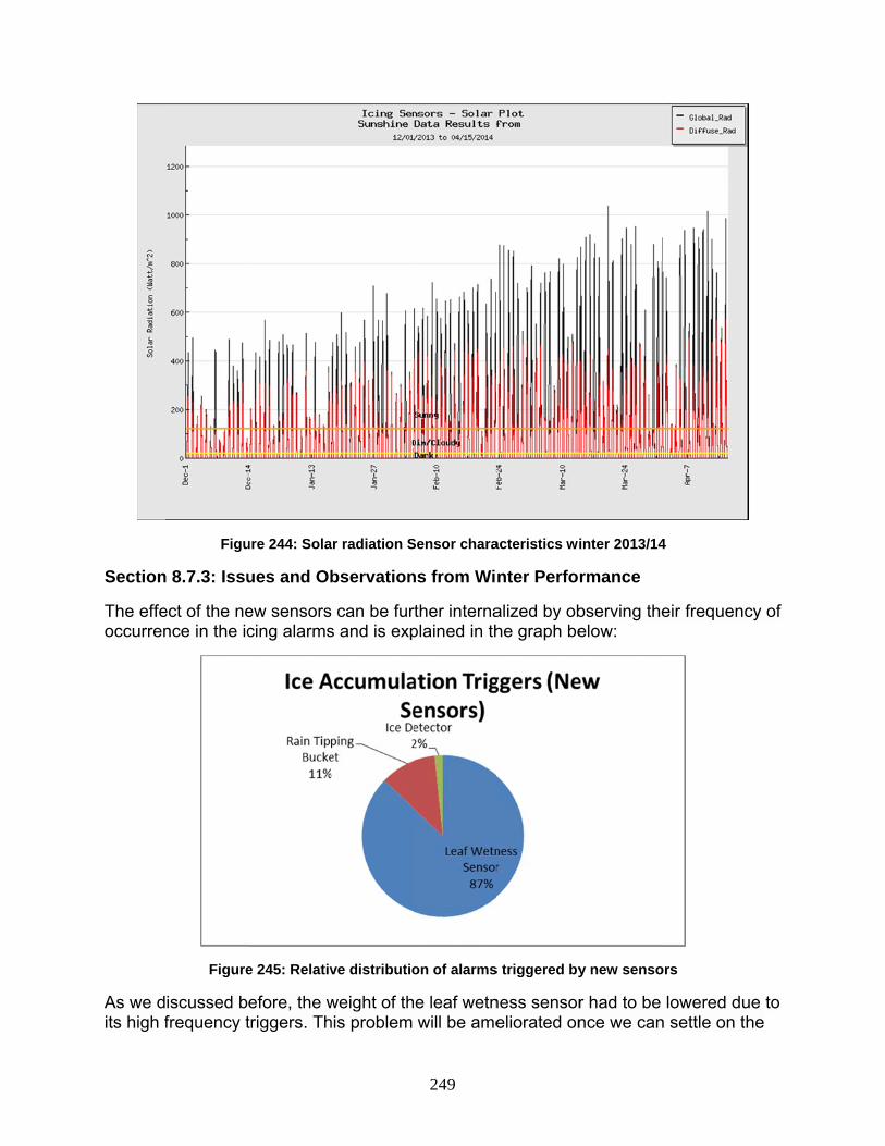
Section

The effeoccurren

As we dits high f

Figu

n 8.7.3: Issu

ect of the nence in the ic

Figure

iscussed bfrequency t

ure 244: Sola

ues and Ob

ew sensorscing alarms

e 245: Relativ

efore, the wtriggers. Th

ar radiation S

bservation

s can be furs and is exp

ve distributio

weight of thhis problem

249

Sensor chara

ns from Wi

rther internaplained in th

on of alarms

e leaf wetnwill be ame

acteristics wi

nter Perfo

alized by obhe graph be

s triggered by

ness sensoreliorated on

inter 2013/14

rmance

bserving theelow:

y new senso

r had to be nce we can

4

eir frequenc

ors

lowered dun settle on t

cy of

ue to he

250

most appropriate threshold value for the sensor. The rain bucket being down most of the season also does not have a large share of the dashboard triggers. The ice detector set the alarm off only twice as it has a high threshold of 0.05 inches. Since this device is primarily being used for ice determination and not thickness in the algorithm, we could either lower its threshold ( although about 0.2 inches ice or more is considered hazardous) or quickly send our warning level to Y2 (secondary alarm for accumulation).

For example, the icing event of April 3rd occurred after only a few hours, which in comparison to previous events was relatively quickly. We did not reach Y3, which requires persistence of icing conditions for several more hours. One possible solution to this faster icing scenario is to define another threshold for the icing sensor that would push us to Y3 immediately regardless of the normal alarm algorithm. This would override the normal process in cases of fast accumulation of ice as on April 3rd.

Similarly, for ice shedding sensors – stay thermistors and solar radiation sensor, the individual sensor threshold flag was set numerous times, but we do not have any useful data for deliberation as the overall shedding conditions were not met and hence the shedding alarms were not triggered.

If we look back at table 17, there have been many events were the remote weather stations missed an event but the new icing sensors caught them and vice versa. There is no doubt that introduction of the new sensors have strengthened our dashboard algorithm by complementing & supplementing the existing remote weather stations with redundancy. The ultimate goal is to have as many sensors reporting similar icing conditions accurately and eliminate any requirement of human intervention.

Despite their minor shortcomings which can only be improved by our learning of their long term characteristics, the new sensors have provided us much more redundancy and control over our dashboard algorithm. Tuning the dashboard algorithm most accurately would depend upon these sensors’ performance and their longevity, and these can be better validated with time and a larger training set.


A new sensor suite has been deployed on the VGCS bridge. These include:

Geokon Thermistor 3800-2-2, for stay surface temperatures

Decagon LWS-L Dielectric Leaf Wetness Sensor, for detecting water/moisture with some classification as ice, light rain/snow, or heavy snow/rain.

Delta-T Devices Sunshine Sensor BF5, for detecting and quantifying solar radiation and approximate level of cloud cover

Met One Rain Tipping Bucket, for detecting and quantifying precipitation

Goodrich Ice Detector, for detecting and quantifying ice thickness

251

In addition, the dashboard has been modified to account for and utilize these new sensors for predication of ice accumulation and shedding. The following objectives for phase II have been successfully implemented.

New module has been added in the algorithm to test the functioning of all the remote weather stations. This monitor of the monitor concept can be viewed through a new table in dashboard main panel which reports station status as green (working) or red (not working).

To increase the speed, redundancy and accuracy of the algorithm we installed different icing sensors such as stay thermistors, ice detector, dielectric leaf wetness sensor, rain tipping gage, solar sensor etc. on the bridge location itself

In order to decide ice events more accurately, there are some parameters that are critical, such as solar radiation, type of wetness, thickness of ice etc. New sensors now provide us this data.

As we have active control over our data logger programs scheduling data collection, we can now change different thresholds, sampling rates etc. as per our requirements.

As we required a much faster system to catch quick ice shedding incidents, our local sensor system can now collect data in seconds, if required.

252

Chapter 9: Ice Presence and State Sensor Development


There is no commercial available sensor for the ice presence and state. There are two primary motivations for developing this sensor.

1) The Goodrich ice detector cannot sense ice persistence. The ice detector can detect the accretion of ice and by using an integration strategy to adjust for the ice detector heating cycles can estimate the initial thickness of the ice (Ryerson has a paper on this. It could be cited here.). However, the ice may sublimate or fall off the sensor tip before it releases from the stay. Thus, the ice detector has limited utility in revealing ice persistence.

2) Liquid water beneath the ice is a precursor to ice shedding. Coupled with stay surface temperature from the stay thermistors, recognizing the presence of water beneath the stays is expected to be a powerful predictor of imminent shedding. Such knowledge would give ODOT time before a shedding event to change the traffic patterns.

Therefore, an effort to develop an ice presence and state sensor was undertaken. A simple resistance based sensor was developed. Laboratory and outdoor tests were successful in differentiate the state of water on the sensor as it changed leading up to an experimental ice shedding event. The sensor cannot reliably provide an indication of the thickness of the ice. The sensor is ready for deployment.

Section 9.2: Ice Presence and State Sensor Laboratory Testing

The Ice Presence and State Sensor (hereafter referred to as the “UT icing sensor”) was successfully developed using the differences in the electrical resistance properties of water, ice, and slush. Pure water will not conduct electricity to any measurable degree. However in naturally occurring water, the impurities in the water permit some conduction. Ice can also conduct electric current like water. But the conductivity is much reduced because the ion motion through the solid is thousands of times smaller than the motion of the same ions in the liquid water. Therefore, water is a much better conductor than ice. Finally, slush, which is the mixture of water and ice, is also conductive. It does not allow conduction as well as water, but permits much more conduction than ice. By using this basic property (conductivity), this sensor can detect the state of a medium whether it is water, ice, or slush.

Section 9.2.1: Sensors and Data Acquisition System

Conductivity is the reciprocal of resistivity: conductivity = 1/resistivity. Therefore, it is inversely proportional to resistance. UT icing sensor is developed to detect the resistance of a medium present on the surface of the sensor. Figure 246 shows the schematic circuit of the UT icing sensor. R1, R2, Eo, and Ei represent the fixed resistor, variable resistor, output data, and input voltage, respectively. R2, also called electrode spacing, is the area where sensor detects the state of a medium as seen in Figure 247.

Th

Eo is coconnecte

As seenthermoccriteria hconsiderbe wateconsider

Nationalsensor atransferrdevices and shotemperarule. It arules areand betw

hermocou

nnected to ed to a pow

in figure 24couple playshas been crred to be icr. And finallred to be sl

l Instrumenas shown inred throughrespectivelws the data

ature limit foalso shows te mentionedween 2 and

ple

data acquiswer supply w

F

Figure 247:

47, a K-types a very impreated as if e. If the temly, if the temush.

t devices wn Figure 248h NI USB-TCy. Both dev

a on its dasor ice and lothe possibled before, if

d -2°C, it is c

sition systewhich provi

igure 246: U

Electro Spac

e thermocoportant rolethe temper

mperature omperature o

were chosen8. The tempC01 Thermvices are cohboard as s

ow temperae state of ththe temperconsidered

253

em which trades a direc

T Icing Sens

cing Area of

ouple is attae in determinrature of theof the mediuof the mediu

n for the datperature daocouple Me

onnected toshown in F

ature limit fohe medium rature of the to be ice, w

Electro Sp

ansfers datct current of

sor Circuit

the UT Icing

ached to thening the stae medium isum is aboveum is betwe

ta acquisitioata and resieasuremen

o a LabViewigure 249.

or water canwhether it

e medium iswater and s

pacing

Variable R

a to a compf 5 Volts.

g Sensor

e UT icing sate of a meds below -2 e 2 °C, it is een -2 and

on system fstance data

nt and NI USw program wIn the dashn be set accis water, slus below -2 °slush respe

Resistor (R

puter. Ei is

sensor. Thisdium. The °C, it is considered2 °C, it is

for the UT ia are SB-6210 which interp

hboard, the cording to tush, or ice. °C, above 2ctively. In

R2)

s

d to

icing

prets high

the The

2 °C,

additiontemperadata into

Section

The purpwater, s°C. The known toFigure 2respectiv

NI USB

, the dashbature (°C) aco an excel f

Figur

n 9.2.2: Des

pose of thelush and iceresistance o have lowe

250 and 251vely.

-6210

board preseccording to files once th

re 248: UT Ici

Figur

sign of Exp

initial expee. All measof ice is knest resistan1 shows UT

nts the reatime (s). T

he user click

ing Sensor C

re 249: Dash

periments

eriment wasurements aown to be t

nce. The exT icing sens

254

l time plots he dashboaks on the st

Connected to

hboard of UT

s to measurare done in the highest periment is

sor with 1-m

of resistanard is also atop button.

o Data Acqui

Icing Senso

re resistanca controlledof all, on th

s done usingmm and 7-m

ce (kOhm) automatica

sition Syste

or

ces for threed room temhe other hag two UT ic

mm electro s

NI USB

UT Ici

DirectSuppl

and lly saved th

m

e mediumsmperature a

nd, water iscing sensorsspacing

B-TC01

ng Sensor

t Current Py

he

; t 22 s s.

r

Power

Figure 2

The UT Then, icmediumthan memeasurecorrespotested; 7mixture (LWC) oand 50%slush whLWC of

50: 1-mm EleSe

icing sensoe, slush, an. Figure 252

easuring theed. Water aonding to w75% slush, of 75% ice

of all the slu% water. Thhich is the mall the slus

ectro Spacinensor

or and thermnd water are2 and 253 s

e resistanceand ice are weights of ic

50% slush,and 25% w

ushes. Figuris type of s

mixture of 2hes.

1 m

ng UT Icing

mocouple we filled in thshows watee of water ablended in

ce and wate, and 25% s

water. This tre 255 showlush has m

25% ice and

mm

255

Figure 251

were glued ohe containeer and ice mand ice, slusthe curtain

er. In this exslush. Figurtype of slusws 50% sluedium LWC

d 75% wate

1: 7-mm ElecSen

onto the bor to measur

measuremesh’s resistaratio to ma

xperiment thre 254 showsh has the leush which isC. And finaler. This type

ctro Spacingsor

ottom of a pre the resis

ent respectivnce is also

ake slush. Three types ws 75% slueast liquid ws the mixturlly, Figure 2e of slush h

7

g UT Icing

lastic contastance of eavely. Other to be

This ratio is of slush are

ush which iswater contere of 50% ic256 shows 2as the mos

mm

ainer. ach

e s the ent ce 25%

st

F

Figu

Furthermmediumexamplethe thickmeasure

igure 252: W

ure 254: 75%

more, the m: 6 mm (0.2

es of measuknesses andement. The

Water Measur

% Slush Meas

Fig

measuremen25 in), 13 muring resistad the mediu similar fas

rement

surement

gure 256: 25

nts were mamm (0.50 in)ance of ice um needs tohion measu

256

Fig

5% Slush Mea

ade for thre), and 19 mfor three tho be filled uurements w

Figure 253:

gure 255: 50%

asurement

ee different m (0.75 in)

hicknesses.up to the linwere also do

: Ice Measure

% Slush Mea

thicknesse). Figure 25 The blue lie to get an one for wate

ement

asurement

es in each 7 to 259 shines represaccurate

er and slus

hows sent

h.

Figure

Section

UT Icingmeasurecan be s

e 257: Ice Methic

n 9.2.3: Lab

g Sensor wements wasseen in Figu

easurement ackness

Figure 2

boratory Te

with 1-mm s done usinure 250. Th

at 6 mm

59: Ice Meas

est Results

Electrode ng UT icing he results ar

257

Figure 2

surement at 1

s

Spacing. Tsensor withre shown b

258: Ice Measthickn

19 mm thickn

The first seth 1-mm eleelow.

surement at ness

ness

t of resistanctrode spac

13 mm

nce cing, the seensor

The figucorrespomelt at rhigh as ashows thstate” se

Resistance (Ohm)

Fig

re above shonding to teroom tempeapproximathe screenshection show

0

500000

1000000

1500000

2000000

2500000

3000000

3500000

4000000

‐10

()

ure 260: Res

hows compemperatureserature. Thetely 3,500 khot of the m

ws that ice is

Figure 261:

‐8

sistance of Ic

parison of res. Three mee ice which kOhm and amonitor whils detected (

Dashboard

‐

Tempera

258

ce for 1-mm

esistances easuremenhas a temp

as low as ape measurin(as indicate

Screenshot

6

ature ( C)

Electro Spac

of ice in thrnts were donperature ofpproximateng the resised by the re

of Ice Measu

‐4

cing Sensor

ree differenne while let-2 °C has r

ely 200 kOhstance of iceed arrow).

urement

‐2

6 m

13

19

~200

t thicknessetting the iceresistance am. Figure 2e. The “pos

mm Thickness

mm Thickness

mm Thickness

0000

es e as 261 ssible

Figure 2correspotempera°C has rkOhm. Tthat has dashboashows th

Resistance (Ohm)

Figure

262 shows conding to timature for 120resistance aThe resistan

a higher liqard while mhat slush is

Fig

0

10000

20000

30000

40000

50000

60000

70000

80000

0

262: Resista

comparisonme. Three m0 seconds. as high as ance drop sequid water ceasuring th detected.

ure 263: Das

20 40

ance of 75% S

n of resistanmeasuremeThe slush w

approximateeen in the gcontent (LWhe resistanc

shboard Scre

60

Time (s)

Res

259

Slush for 1-m

nces of 75%ents were dwhich was ely 70 kOhmraph shows

WC). Figurece of 75% s

eenshot of 7

80 100

sistance Dro

mm Electro S

% slush in thdone while lat a tempem and as los that the s

e 263 showsslush. The p

5% Slush Me

120

op

Spacing Sen

hree differeletting slushrature rangow as approensor detecs the screepossible sta

easurement

75% Slush 6

75% Slush 13

75% Slush 19

sor

ent thicknesh melt at ro

ge of -2 andoximately 1cts part of snshot of the

ate section

mm Thickness

3 mm Thickness

9 mm Thickness

sses om 2 0

slush e

Figure 2thicknesmeasureThe slusapproximresistancthat timeexposesmeasuridetected

Figure

264 above ssses correspements wersh which wamately 1,30ce drop whe. The 50%s to a very hng the resisd.

Fig

0

200

400

600

800

1000

1200

1400

0

Resistance (Ohm)

264: Resista

shows compponding to re done whas in a temp00 Ohm andich means slush of 13high LWC. Fstance of 50

ure 265: Das

20 40

ance of 50% S

parison of rtime. Similaile letting slperature rad as low as the sensor

3 mm thicknFigure 2650% slush. T

shboard Scre

0 60 80

Time (s)

260

Slush for 1-m

resistances ar to the preush melt atnge of -2 anapproximatdetects the

ness showsshows the

The possibl

eenshot of 5

0 100 12

ResistancDrop

mm Electro S

of 50% sluevious expet room tempnd 2 °C hastely 250 Oh

e part of slus low resistascreenshote state sec

0% Slush Me

20

50%

50%

50%

ce

Spacing Sen

ush in threeeriment, thrperature fors resistancehm. It also sush that hadance becaut of the das

ction shows

easurement

% Slush 6 mm Th

% Slush 13 mm T

% Slush 19 mm T

sor

different ree r 120 secone as high asshows d higher LWuse the senshboard wh that slush

hickness

Thickness

Thickness

nds. s

WC at sor ile is

Figure 2corresporoom tem2 °C hasOhm. Ththat has this typewhile meslush is

Resistance (Ohm)

Figure 2

266 shows conding to timmperature fs resistancehe resistanchigher LW

e of slush haeasuring thdetected.

Fig

0

50

100

150

200

250

300

0

66: Resistan

comparisonme. Three mfor 120 sece as high asce drop see

WC. The 25%as very highe resistanc

ure 267: Das

20 40

nce of 25% S

n of resistanmeasuremeonds. The ss approximaen in the gra% slush at ah LWC. Fige of 25% sl

shboard Scre

60

Time (s)

R

261

lush for 1-m

nces of 25%ents were dslush whichately 270 Oaph shows all thicknessgure 267 shlush. The p

eenshot of 2

80 100

Resistance D

m Electrode

% slush in thdone while lh is in a temOhm and as

that the seses shows ows the sc

possible stat

5% Slush Me

120

Drop

e Spacing Se

hree differeletting slush

mperature ras low as appensor detectlow resistanreenshot ofte section s

easurement

25% Slush 6 m

25% Slush 13

25% Slush 19

nsor

ent thicknesh melted in ange of -2 aproximatelyts part of slnce becausf the dashbshows that

mm Thickness

3 mm Thickness

9 mm Thickness

sses a

and y 250 ush se board

The grapthicknestemperaresistancthis casethroughothe resis

Resistance

(Ohm)

Figu

ph above ssses correspature for 120ce as high ae, there is nout its bodystance of wa

F

0

50

100

150

200

250

0

Resistance (Ohm)

re 268: Resis

hows compponding to 0 seconds. as approxim

no presencey. Figure 26ater. The p

Figure 269: D

20 40

stance of Wa

parison of retime. ThreeThe water

mately 207 e of resistan69 shows thossible stat

Dashboard S

60

Time (s)

262

ater for 1-mm

esistances e measuremwhich is in Ohm and ance drop bee screenshte section s

creenshot of

80 100

m Electro Spa

of water in ments werea temperat

as low as apecause wathot of the dashows that w

f Water Meas

0 120

acing Senso

three differe done in a rture range approximateter has unifoashboard wwater is det

surement

Water 6 m

Water 13 m

Water 19 m

or

rent room above 2 °C

ely 188 Ohmorm proper

while measutected.

mm Thickness

mm Thickness

mm Thickness

C has m. In rty uring

263

UT Icing Sensor with 7-mm Electrode Spacing. The second set of resistance measurements was done using UT icing sensor with 7-mm electrode spacing, the sensor can be seen in Figure 251. The same procedure was performed as 1-mm electrode spacing sensor. The results are shown in the following figures.

Figure 270: Resistance of Ice for 7-mm Electro Spacing Sensor

Figure 271: Resistance of 75% Slush for 7-mm Electro Spacing Sensor

0

1000000

2000000

3000000

4000000

5000000

6000000

‐8 ‐7 ‐6 ‐5 ‐4 ‐3 ‐2

Resistance (Ohm)

Temperature ( C)

6 mm Thickness

13 mm Thickness

19 mm Thickness

0

20000

40000

60000

80000

100000

120000

140000

160000

180000

200000

0 20 40 60 80 100 120

Resistance (Ohm)

Time (s)

75% Slush 6 mm Thickness



Resistance Drop

264



Figure 274: Resistance of Water for 7-mm Electro Spacing Sensor

0

100

200

300

400

500

600

700

0 20 40 60 80 100 120

Resistance (Ohm)

Time (s)




0

50

100

150

200

250

300

350

0 20 40 60 80 100 120

Resistance (Ohm)

Time (s)




200

205

210

215

220

225

230

235

240

245

250

0 50 100

Resistance (Ohm)

Time (s)

Water 6 mm Thickness



265

The result of 7-mm electro spacing sensor shows very similar trend compared to the previous experiment. The resistance of ice is the highest of all, above 400000 Ohm. On the other hand, the resistance of water is the lowest and that of slush is in between. The slush’s resistance depends on its LWC. The result indicates that the higher LWC, the lower the resistance as seen in the result of 25% slush having lower resistance than 50% and 75% slush respectively. Figure 275 is provided to present resistances of all mediums at the 6 mm thickness and 7 mm electro spacing. It clearly shows that each medium has its own resistance range and this trend is similar for other cases.

Figure 275: Resistances for 6-mm Thickness and 7-mm Electro Spacing Sensor

However, the results show that the resistance is not dependent on the thickness of a medium. By analyzing Figures 270 to 274, it appears that the thickness does not play a significant role in the medium’s resistance. Overall, the result from this experiment is very valuable and was be applied to the full scale experiment which will be discussed in the next section.

Section 9.3: UT Icing Sensor in Full Scale Experiments

Since the performance of the UT icing sensor in the laboratory was promising, the sensor was installed in a full scale experiment. The goal of experiments was to simulate the ice and wet snow formulation on the specimens and track the behavior of those mediums in the more realistic environment. The full scale experiment was initially designed in winter 2012-2013. For the efficiency and safety issues, the experiment station was located at the Scott Park campus of the University of Toledo instead of at the VGCS. Three 10 ft-long cable stay sheath with the same diameter and material as the VGCS stays have been set up as shown in Figure 276. In winter 2013-2014, a high density polyethylene (HDPE) specimen from another bridge was added to the experiment station as seen in Figure 277. Ice and wet snow experiments were performed at this experiment station.

100

1000

10000

100000

1000000

10000000

0 20 40 60 80 100 120

Resistance (Ohm)

Time (s)

Ice

75% Slush

50% Slush

25% Slush

Water

Section

At the expad. All concrete276 reprspecimeas sameorientatitensionesimulate

HDP

n 9.3.1: Spe

xperiment sthree speci

e blocks to resenting seens are facie as the orieon which w

ed strands pe the bridge

PE Specimen

Figure

Figure 27

ecimens an

station, the imens are ahave approemi-steep sng in differeentation of t

will be discuplaced insid

e conditions

e 276: VGCS

77: HDPE Sp

nd Data Ac

three VGCalign from Noximately 30stay-cablesent directionthe VGCS bss in the rede the North as realistic

266

Stainless St

pecimen and

cquisition S

S specimenNorth to Sou0 degree anat VGCS b

n, one facinbridge. Thesult of this h facing specally as pos

teel Specime

Frame Struc

System Se

ns have beuth and twongle to the bridge. Theng North ane sun radiatchapter. Figecimen. Thssible.

ens

cture

etup

en set up oo of them arground as sse two sup

nd the othertion has an gure 278 shis experime

Frame

on a concrere supporteseen in Figported r facing Soueffect on thhows 120 uental setup

e Structure

te ed by ure

uth, his un-is to

The HDPin a simiHDPE sangle to ultrason

The UT specimeas showsensor issensors representhe sensdiscoverinformat282 sho

F

PE specimeilar orientatpecimen suthe groundic and thick

icing sensoens. The sewn in Figures installed oare placed

nts the crossors were sred along thtion will be vws the UT

Figure 278: N

en had a diion as the Supported byd. The framkness senso

ors developnsors weres 279 and 2on the top p on East, T

ss section oet up as shhe circumfevery helpfuicing senso

North Facing

ameter of 2South faciny concrete be structure ors, for mor

ed in a laboe installed a280. Figurepart of the HTop, West, aof a specimehown is becerence of thl to determi

or attached

267

Specimen w

20 centimetg VGCS spblocks so it was built to

re data colle

oratory werapproximatee 280 also sHDPE specand Bottomen and its sause the the specimenine ice or snto the surfa

with 120 Stan

ters. The Hpecimen. Fi

makes appo be able toection durin

re installed ely at the mshows that tcimen. Four

m sides of easensors sethermal propns while icenow accretace of HDP

nds Inside

DPE specimgure 277 sproximatelyo install senng the expe

on both VGid-span of bthe dielectrr sets of theach specimtup orientatperties are ne or wet snoion and she

PE specimen

Strands

men was sehows the

y 30 degreensors, such eriments.

GCS and HDboth specimric leaf wetne UT icing

men, Figure ion. The reaneed to be ow occurs. Tedding. Figun.

et up

e as

DPE mens ness

281 ason

This ure

Figur

The UT used in t

UT Ic

Thermoco

re 279: SensSpe

Figure 28

icing sensothe laborato

ing Sensors

ouple

ors Setup onecimen

1: Cross Sec

Figure 2

ors tested inory. Howev

West

n VGCS

ction and Sen

282: UT Icing

S

n the full scver, a differe

t

UT Icin

268

Figure

nsor Setup O

g Sensor on H

Specimen

ale experiment the data

Top

Bottom

g Sensors

e 280: SensoSpec

Orientation o

HDPE Specim

ments were a acquisition

East

ors Setup on cimen

of both Spec

men

the same an system w

LWS

HDPE

imens

as the oneswas used. T

s The

Scott PaMicroStrfeature iMicroStrthe labosystem psensor cicing sendata of bacquisitithermoc

Fi

AccordinEo, and respectiv

R1 and respectivThe equ

ark data acqrain data acs very convrain V-Link ratory test iprovides 7 circuit. The nsor is alsoboth sensoron system.

couples are

gure 283: Mi

ng to the scEi represenvely. The e

Ei are desigvely. The o

uation befor

quisition syscquisition syvenient for tand TC-Linis connectemVDC andcommercia

o connectedrs. The Mic It works wchosen for

icroStrain V-

chematic cirnts fixed requation of t

gned to be utput voltag

re can be fu

stem recordystem werethis type of nk respectived to MicroS was set to

al LWS whicd to the MicrroStrain TCith any typer this experi

-Link

rcuit of the sistor, variathe sensor

fixed whichge (Eo) is durther simpl

269

ded voltagee selected b

experimenvely. The saStrain V-Lin read the voch has simiroStrain V-L

C-Link is a we of thermocment.

Figu

UT icing seable resistocircuit is sh

h in this casdepended oified as:

1

e rather thabecause it isnt. Figures 2ame UT icinnk directly. Toltage outplar electricaLink to be awireless thecouple in w

ure 284: Micr

ensor shownr, output da

hown below

se, there areon what dete

n resistancs wireless. 283 and 284ng sensor cThis data a

put from theal mechanisable to comermocouplewhich K-type

roStrain TC-L

n in Figure ata, and inp

w.

e 1 kOhm aected on th

ce. The newThe wireles4 shows

circuit built fcquisition

e UT icing sm as the U

mpare the ree data e

Link

246, R1, Rput voltage

and 7mV e sensor (R

w ss

for

UT esult

R2,

R2).

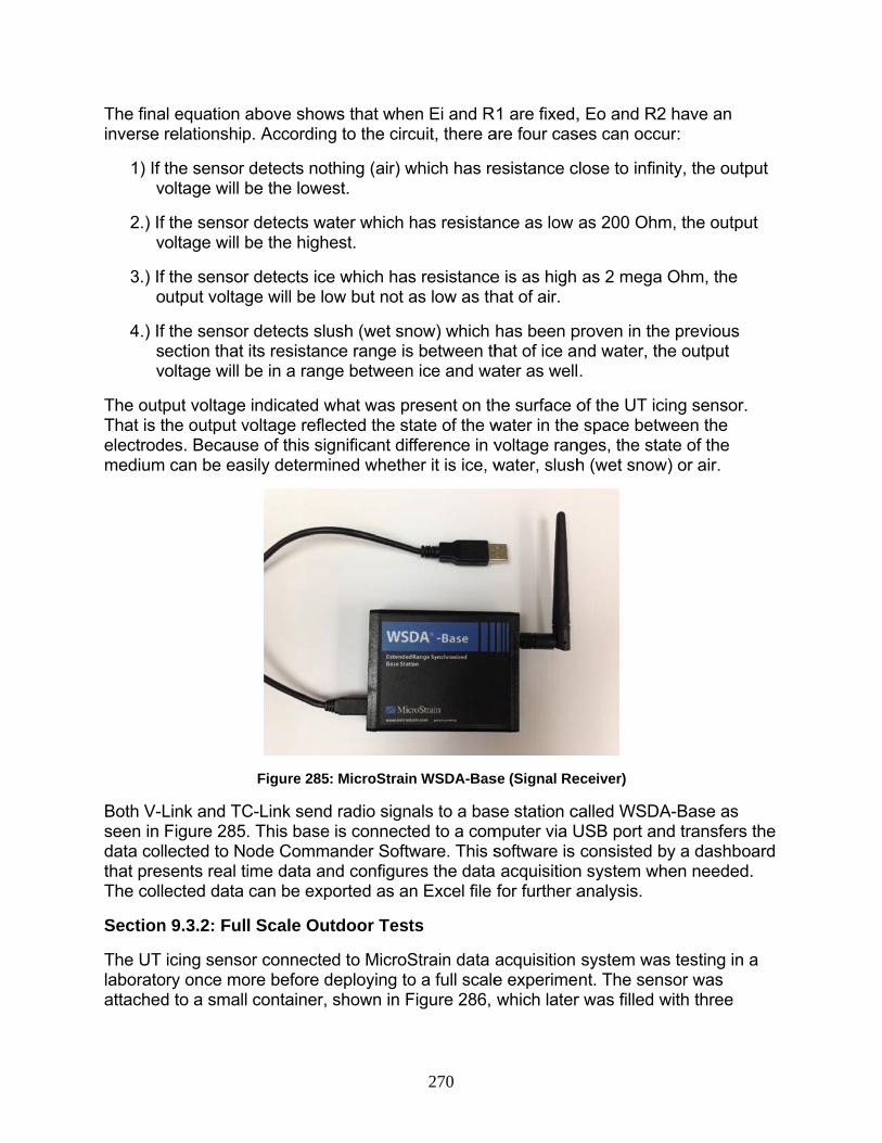
The finainverse

1) If tv

2.) If v

3.) If o

4.) If sv

The outpThat is telectrodmedium

Both V-Lseen in data colthat presThe colle

Section

The UT laboratoattached

al equation arelationship

the sensor oltage will b

the sensoroltage will b

the sensorutput voltag

the sensorection that oltage will b

put voltage he output ves. Becaus can be eas

Link and TCFigure 285.lected to Nosents real tiected data

n 9.3.2: Ful

icing sensoory once mod to a small

above showp. According

detects notbe the lowe

r detects wabe the highe

r detects icege will be lo

r detects sluits resistanbe in a rang

indicated wvoltage reflese of this sigsily determi

Figure 285

C-Link send. This base ode Commime data ancan be exp

l Scale Ou

or connecteore before d container,

ws that wheg to the circ

thing (air) west.

ater which hest.

e which hasow but not a

ush (wet snce range isge between

what was prected the stgnificant difined whethe

: MicroStrain

d radio signais connecteander Softwnd configureported as an

tdoor Test

ed to MicroSdeploying toshown in F

270

en Ei and Rcuit, there a

which has re

has resistan

s resistanceas low as th

ow) which s between thn ice and wa

resent on thtate of the wfference in ver it is ice, w

n WSDA-Bas

als to a based to a comware. This ses the datan Excel file

ts

Strain data o a full scaleFigure 286,

1 are fixed,are four cas

esistance c

nce as low

e is as high hat of air.

has been phat of ice aater as well

he surface owater in thevoltage ranwater, slush

se (Signal Re

se station cmputer via Usoftware is

a acquisitionfor further a

acquisition e experimewhich later

, Eo and R2ses can occ

close to infin

as 200 Ohm

as 2 mega

proven in thnd water, th.

of the UT ice space betwnges, the stah (wet snow

eceiver)

called WSDAUSB port anconsisted b

n system whanalysis.

system want. The sen

r was filled w

2 have an cur:

nity, the out

m, the outp

a Ohm, the

e previous he output

cing sensorween the ate of the w) or air.

A-Base as nd transfersby a dashbohen needed

as testing innsor was with three

tput

put

r.

s the oard d.

n a

differentstate.

Figure 2while co

t states of m

287 to 289 sollecting sen

Figure 28

medium (ice

Figu

shows ice, snsor output

87: Ice Testin

e, slush, and

ure 286: V-Li

slush, and wdata.

ng

Figure 28

271

d water) to

ink and UT Ic

water on th

89: Water Te

determine

cing Sensor

e surface o

Figure 28

sting

an output v

of the UT ic

88: Slush Tes

voltage of e

ing sensor

sting

each

The resua characshows aThe outpwater, it figure. Athe presranges.

Section

During wand wet the winte2013). Texperimthe winte

Icing Exnights, tspecimeraise theice pattehours. T

ultant data fcteristic rana very low raput range ohas a non-

As resulted, sence of me

n 9.3.3 Full

winter of 20snowing m

er of 2012-2This thesis fent. In addier of 2013-2

xperimentshe ambient

en as seen e specimenern accumuThe ice thick

from this tege of outpuange, but n

of slush was-uniform proall four sta

edium on th

Fig

Scale Exp

12 to 2014methods. Icin2013 have focuses on ition, wet sn2014 is also

s: The expet temperatuin Figure 29 temperatulated on the

kness was m

esting is preut. The rangot as low a

s between woperty whictes clearly e surface o

ure 290: UT

periments R

, multiple fung experimbeen presethe data conow experimo discussed

eriments were was -2 to91. This care above 0°e specimenmeasured t

272

esented in thge of water s a dry surfwater and icch results inhave differe

of the senso

Icing Sensor

Result

ull scale expent on VGC

ented and dollected via ments on Hd in this the

ere performo -15 °C. Wused the la°C (Arbabzn after mistito be appro

he Figure 2is very highface (air bece. Since it

n inconstantent ranges or can be ea

r Initial Test

periments wCS specimediscussed bUT icing se

HDPE and resis.

med at the SWater was matent heat ofadegan 20ng water fo

oximately ½

290. Each mh, on the ot

etween the eis a mixture

t output as of data outasily determ

were done, en which w

by Ali (Arbabensor from result which

Scott Park smisted slowf transform13). Figure

or total time½ inch.

medium shother hand, ielectrodes)e of ice andshown in thput. Theref

mined by th

including icas done dubzadegan the icing

h were done

site on cold ly on the VGation not to292 shows

e of 8 to 10

ows ce ). d he fore, e

cing uring

e in

GCS o s the

During tSince thinto the range pewider tha

his experime slush stasensor circermitted a man that foun

Figure

Figure 29

ment, the date was not uit to expanmore sensitnd in the ini

291: Misting

92: Ice Accu

ata acquisititaken in acnd the voltative indicatioitial laborato

273

g Water on V

mulation on

on system ccount, a higage range thon of the icory test and

VGCS Specim

VGCS Spec

monitoredgher fixed rhat could be

ce state. Thed Figure 29

men

cimen

the behavioresistor (R1)e sensed. Ie range of

90.

or of the ice) was placencreasing tice state is

e. ed the

274

Figure 293: Stay Behavior in Icing Experiment

The UT icing sensor and thermocouple data for icing experiment on February 16th, 2013 are presented in Figure 293. Part A in the figure shows the sensor output before starting the experiment. The icing sensor output was very low because it did not detect anything but air. The thermocouple showed the temperature of the stay which is as same as the ambient temperature.

Part B focuses ice accumulation scenario. The cool water was misted starting around 5:00 AM, the UT icing sensor output shows suddenly increase due to the presence of water. Similar to the thermocouple, the temperature rises up to zero degree because of latent heat during the ice transformation. The UT icing sensor output and temperature then gradually dropped because the surface of the specimen was covered with ice. Even though the water was kept misting on the specimen and more ice built up, the sensors were not able to sense that because it can only sense what happen at the surface of the specimen. The misting was stopped before sunrise which was around 7:30 AM.

Part C illustrates ice melting due to a sun radiation scenario. The sun rose around 7:45 AM. The sun radiation had significant impact on the specimen temperature. As sun rose, the specimen and increased as well. However, the ambient temperature was constant throughout that day at -2 °C. Around 10:00AM, ice sheet on the specimen started to melt due to the rise of specimen temperature. This created small water layer between ice sheet and the surface of the specimen. Again the thermocouple shows the latent heat during ice transformation. But this time, the ice turned to water. The UT icing sensor also clearly showed that it detected the presence of water. The change in specimen temperature caused the presence of ice and water throughout the day. However, the

‐20

‐15

‐10

‐5

0

5

10

15

20

0

5

10

15

20

25

30

35

40

02/16/2013 00:00

02/16/2013 03:00

02/16/2013 06:00

02/16/2013 09:00

02/16/2013 12:00

02/16/2013 15:00

02/16/2013 18:00

02/16/2013 21:00

02/17/2013 00:00

Raw

Data (Icing Sensor)

Time

UT Icing

Thermocouple

A B C D

275

specimen temperature was not high enough for shedding event. The ice sheet was still on the surface of the specimen at the end of the day.

After sunset, the ambient temperature sudden decreased as shown in part D. This caused the specimen temperature to drop as well as. The output of the UT icing sensor indicated the presence of ice without water at the surface.

Comparison of the ice accumulation monitoring and UT icing sensor data shows that the sensor reliably reports the presence of ice on the specimen surface. when no natural icing events occurred and the results appeared to be very similar.

Section 9.4: Conclusion and Next Steps

A sensor that can differentiate between ice and water on the VGCS stays has been developed. There is no similar commercial senor. The sensor is rugged and compact so it can be mounted directly on the stay. In an icing event, it will be covered by the ice and detect the presence of liquid water in the interstice between the ice layer and the stay sheath. When there is water in this space, ice fall is imminent. The sensor has been tested in the laboratory and on full scale mock-ups of the VGCS sheath outdoors. The next step is to deploy the sensor on the bridge and integrate it into the dashboard.

276

Chapter 10: Transition and Maintenance


In spring 2014, the dashboard had reached a stage of development where it was appropriate to transfer it to District 2. This transition was organized in a way that the District will able to operate the dashboard through the winter of 2014-2015 and beyond.

The form of transition that was agreed to was a standalone computer at ODOT’s Northwood Output. The Northwood Outpost is the operations center for the VGCS. Shift supervisors. The shift supervisors work with the D02 Highway Management Administrator to make the decisions concerning the response to actual and potential icing events. Therefore, this arrangement puts the Dashboard information at the fingertips of the decision makers.

The standalone system is a static system. The configuration was locked and operational at the time of transfer. Copies of all documents and the user manuals for the sensors have been given to ODOT. This user manual will be permanently archived with this report on the ODOT Office of Research Website the current link is http://www.dot.state.oh.us/Divisions/Planning/SPR/Research/reportsandplans/Pages/default.aspx. Loss of power or modifications to the system may result in loss of functionality.

Section 10.2: Standalone Computer System

The dashboard was frozen in the spring of 2014 and the version of the dashboard that was current at that time was transferred to a standalone system. The standalone system captures the basic functionality of the Dashboard in a desktop system. The local weather conditions and output from the sensors is going to the dashboard. Output from the camera is going directly to ODOT District 2. Figure 10-1 presents architecture of the standalone system. The “Back End” collects data from the local sensors on the bridge and the weather stations throughout the region. The bridge sensor data comes in via ODOT’s intranet. The regional weather data comes from Weather Underground. The data is operated on by the version of the algorithm that was current in spring 2014. The algorithm is described in Chapter 8.3. The “Front End” takes the output from the algorithm as well as the data stream puts them on the Dashboard. The algorithm output goes to the speedometer user interface and access to view the data directly is through the tabs visible on the Dashboard “Home Page”.

The transition of the standalone system to D02 took place on June 5, 2014. The research team delivered the system to the Northwood Outpost. The research team and ODOT D02 IT configured the system and verified its operation

Section 10.3: Maintenance

ODOT is being trained in the operation of the dashboard and a dashboard user manual to support the transition was developed. The user manual has section on maintenance. The user manual is archived on the ODOT of Office of Research website page for final reports the “subject area” is “structures” the current link for the website is http://www.dot.state.oh.us/Divisions/Planning/SPR/Research/reportsandplans/Pages/default.aspx

277

. The maintenance section describes the activities necessary to keep the standalone system operating. The user manuals for the instruments mounted on the VGCS are stored on the standalone system and may be accessed through the Dashboard.

Figure 294: Floowchart for Stand AAlone System

279

Chapter 11: Conclusion, Benefits, Implementation and Future Work

Under some winter conditions, ice forms on the cables stays of the VGCS. Ice accumulations have been observed at a thickness of 3/4”. The ice accumulation depends on the temperature, precipitation and duration of the storm. The accreted ice conforms to the cylindrical shape of the stay sheath. Thus, as the stays warm, the ice sheds in curved sheets. These curved sheets of ice then fall up to two hundred and fifty feet to the roadway below and may be blown or glide across several lanes of traffic on the bridge deck. The falling ice sheets require lane closures and could present a potential hazard to the traveling public.

Section 11.1: Summary of Goals and Objectives

The overall goal of this research was to assist ODOT in implementing an icing management procedure for the VGCS. This procedure may be active, passive or administrative.

Initially, it was the team’s hope that an existing anti/deicing technology would be identified and implemented. With that in mind, phase I of the project began. After an initial review of anti/de-icing technology guided by the experts at the Army Cold Regions Research and Engineering Laboratory, it became apparent that no off-the-shelf or economically viable solution existed. Thus, the following objectives for the overall project were agreed on:

1) Identify available technologies and procedures that could be used to solve the VGCS icing problem. This requires an assessment the state of the art through a literature review and consultation with the icing experts and examining the advantages, disadvantages, and potential applicability of each identified technology on the VGCS.

2) Identify the most viable solutions. It was expected that the most practical solutions will be novel adaptions or combinations of existing solutions. For each viable solution, it was desired to develop a detailed description of the implementation, to define of required validation testing, (either in situ or offsite), to perform a benefit/cost analysis, to develop a budget for implementation and to define a time frame for implementation.

3) Develop a real-time icing condition monitor. This monitor should present data that tracks icing events in a format that is easy to understand and is useful for managing icing incidents. The monitor should also archive the data. Local condition data that is collected from the bridge should be used to increase the algorithm intelligence and error handling of the monitoring system.

4) Collect data to understand the microclimate and icing behavior of the bridge. The collected information should be sufficient to allow accurate costing of an anti/de-icing technology, resolve uncertainties to reduce the risk of deploying an icing strategy that does not work, and be useful for improving and updating the icing monitor.

280

5) Develop a sensor for determining ice presence and state. No suitable sensor exists. Therefore, development and field testing were undertaken

6) Transition the monitoring and local weather station to ODOT District 2 so that the functionality of the dashboard and the information from the icing sensors is available to the operators of the VGCS.

Section 11.2: Results

1) Past icing events were reviewed, the mechanisms for icing where explored, and the basic conditions that are favorable to icing accretion and shedding were ascertained. The general weather system most often associated with major icing is warm air from the Gulf of Mexico overriding cold air from Canada. This leads to liquid water falling on a cold surface. Historically, roughly two icing events occur each year. Icing on the VGCS occurs when there is general icing in the area. There have been five major icing events on the VGCS. The last of which was in February 2011.

Conditions are favorable for ice accretion when one of the following conditions occurs:

iv. Precipitation with air temperature at the bridge below 32o F, or

v. Fog with air temperature at the bridge below 32o F, or

vi. Snow with air temperature at the bridge above 32o F.

The ice accretion rate is generally slow because during an ice storm precipitation rates are low and much of the water runs off the stays. Therefore, it is expected that it will take over six hours to form an ice layer above the critical thickness of 0.25 in. However, in one instance in the spring of 2014 ice exceeded 0.25 in. in a much shorter time.

Once the ice accretes on the stays and pylon, it may persist until shedding conditions occur. Temperatures above 32o F and/or solar radiation cause ice fall. The ice fall in four of the five previous events was accompanied by temperatures rising above 32o F. If the solar radiation level is high enough, ice can shed at temperatures below freezing (32 o F). If there is ice on the stay, weather conditions that cause ice fall are:

iii. Air temperature above 32o F (warm air), or

iv. Clear sky during daylight (solar radiation).

In February of 2011, copious amounts of water flowing beneath the ice were observed when the outside temperature was several degrees below freezing. This layer of water below the ice is a precursor to ice shedding. There is a greenhouse effect that occurs in the interstice between the stay sheath and accumulated ice when the solar radiation passes through the ice and heat becomes trapped. Ice accretion and shedding do not occur simultaneously.

281

Given the unique features of the VGCS, the paucity of literature directly on point, and the urgency of addressing the problem, an expert team was selected. The expert team was the best way to quickly gain familiarity with the state of the art as well as define testing procedures and identify available test facilities. A research team with expertise in icing, icing instrumentation, icing test facilities, the bridge construction and bridge instrumentation was formed to address ice prevention and mitigation on the VGCS.

The initial technology review was extended to a comprehensive review all technologies that could be identified regardless of their technology readiness level. A matrix of over 70 potential technologies was developed. The matrix describes the advantages and disadvantages of each technology. The broad categories of technologies are chemicals and chemical distribution systems; coatings; pneumatic or electrical expulsive deicing systems; modifying the design of the cables (such as by adding straking); radiant heating; interface heating; high-velocity air, water, or steam; mechanical or manual deicing methods; piezoelectric pneumatic systems; vibration, covers and robotic climbers. Ice detection systems were also reviewed.

2) To simulate icing events and use a test bed for experiments an icing field station was designed and built. It had three full scale sheath specimens ten feet long. One of these specimens included strand. The station had a local weather station and a wireless data acquisition. The initial set of experiments verified that ice accretion and shedding similar to that which occurs on the bridge could be replicated. The icing station was then used for experiments on anti/decing chemicals, anti-icing coating, heat for anti-icing and deicing, and tests of instruments.

3) The technologies that were the most viable were identified. They were:

a. Deicing/anti-icing chemicals which would not present a biohazard when leached into the river such a sodium chloride; agricultural products, such as beet based deicers, and calcium chloride

b. Anti-icing coatings c. Heat. The VGCS stays are mostly hollow so there is a potential to

internally heat the stays.

Experiments to evaluate the efficacy of each viable technology were carried out. The experiments were carried out in an icing wind tunnel and at an icing experiment station which was constructed for this project. The icing experiment station had full-scale stay sheath specimens that were 10 feet long.

The anti-icing chemical experiments showed that on the stainless steel surface of the sheath the chemicals tested did not persist. Therefore, the onset of icing was only slightly delayed. The deicing experiments showed that the chemical tested was not viscous enough to sheet across the sheath surface. Rather it cut groves through the ice and was not effective in removing the ice. These results are consistent with the results in the literature. In addition, to not performing the

282

desired anti/deicing functions, chemicals would require a distribution system so they were deemed impractical.

Several anti-icing coating were tested in the icing wind tunnel and at the icing experiment station. The coatings did not significantly delay the onset of ice, which stuck to the stay specimens and most did not change the shape of ice that shed. The coating that was outdoors for an extended duration of time became opaque and gummy, therefore, it would alter the appearance of the stays. These results are consistent with the results in the literature. Additionally, coating would be difficult to apply so they were deemed impractical.

Introductory heating experiments were carried out at the icing experiment station. The heating was effective and deicing and partially effective at deicing. The temperature of the epoxy coated strand inside the sheath cannot be raised above 150 degrees F, so the initial thermal analysis showed the heating was a slow process. The requirement to heat each stay would require an expensive heating system. At that point, heating was deemed impractical so no advanced experiments or thermal analyses were conducted.

No active or passive system was identified which had sufficient level of promise to justify detailed estimates of installation, operation or maintenance costs.

4) When it was judged that the regional weather information and the RWIS did not provide enough information to assess the microclimate and icing behavior, a local weather station was installed on the bridge. The weather station has five sensors and a weather proof camera. Thermistors are mounted on a stay in the back span and on a stay in the cantilever. A Goodrich ice detector, a solar radiation monitor, a dielectric leaf wetness moisture sensor, heated tipping rain gage and the weather proof, pan, tilt zoom camera are mounted on a weather tower of the south end of the back span. The combination of the existing sensors and the newly added sensors gives a good picture of the conditions on the bridge.

Prior to deployment in the field, experiments on the sheathing specimens at the field station and in the laboratory coupled with the literature review lead to the conclusion that the proposed sensors functioned as desired and they were recommended for installation.

It is especially valuable that the Goodrich ice detector can be used to provide an estimate of the thickness of the icing accumulation. The actual ice accumulation can then be compared to the critical thickness of one-quarter of an inch.

The stay thermistors revealed the temperatures on the stays was significantly different than the RWIS or Metar data. They data both lag the stay temperatures by up to 3 hours or 20 F. This means air temperature is of limited use for assessing shedding.

5) To make the research immediately actionable by ODOT operations, a real-time icing condition monitor was developed. The research team designed a real-time

283

monitoring system to track icing conditions on the bridge with a straightforward interface so information on the icing of the bridge was readily available to the bridge operators. This monitoring system is referred to as the “icing dashboard” or simply “the dashboard” because the information necessary to support ODOT operations is presented on one simple visual display. The dashboard tracks the icing events in a format that is easy to understand, is useful for managing icing incidents and archives data. When conditions favorable to icing occur the dashboard alerted the research team. If the conditions favorable to icing persisted, ODOT was notified and, as required, requests for verification of ice accretion were made.

The primary features that are implemented in the dashboard include:

User friendly check engine lights to monitor ice on the Bridge for:

a. Conditions favorable to ice accretion

b. Conditions favorable to ice shedding

Add weather data to existing VGCS web interface

Add new stay - mounted camera views to existing VGCS weather interface

Develop algorithm to monitor ice events

Develop reporting function for ODOT to verify the alerts and declare an event

Develop export function for historical data archive

Run calibration studies based on historical data

The basis of this system is the smart mix of the automated algorithm and the visual observations, which helped aid in training the system for more optimal performance. The system uses an intelligent decision making process based upon initial criteria from past weather data analysis with parameter adjustments made after visual observations. Dashboard has done well in detecting ice accumulation each time, but the analysis done on the algorithm results and onsite observations from research team members and ODOT have been used to refine the algorithm as well as the interface.

Additionally, local condition data and the review of recorded events that were collected from the bridge were used to increase algorithm intelligence and error handling. The improvements focused on the enhancement of the visual display, refinement of the accretion and shedding algorithms and incorporation of data for a local weather station on the bridge and reducing false alarms.

The dashboard has proven to be a valuable resource for the bridge operators as well as a valuable tool for reviewing weather events. The automated ice

284

detection and monitoring dashboard for the VGCS was developed, implemented, successfully tested, and has been transferred to ODOT.

6) An ice presence and state sensor has been developed. No suitable sensor to detect the continued presence of ice or the transition from ice to water exists. Therefore, development and field testing of a suitable sensor were undertaken. The resistance based sensor detects the presence of ice and can differentiate between ice and liquid water. The sensor is designed to be mounted on the sheath and can detect the layer of water which forms beneath the ice just prior to shedding. The sensor has been tested in the laboratory and at the icing experiment station.

7) The transition of the dashboard to District Two has concluded. A local standalone computer with the dashboard on it has been provided to the District. The standalone version maintains the basic functionality of the dashboard algorithms and alert system and provides links to the icing weather instrumentation on the bridge. A person at the computer can monitor the conditions on the bridge and determine the causes of alerts. The dashboard is a complex system and to maintain the functionality of the dashboard the District should not make any changes to program.

Section 11.3 Benefits

The overall benefit is increased safety for the traveling public. The specific benefits of completing this project were:

The icing events in northwest Ohio for the past twenty years including the first four icing events on the bridge were reviewed. Vehicles were damaged in at least two of the first four icing events.

All of the known anti/de-icing technologies were investigated. The included over 70 technologies. These technologies are described in the technology matrix.

Observations and a detailed study of the February 2011 major icing event were completed. This was the fifth major icing event on the bridge since its opening. The bridge was closed for several hours. The team used the dashboard to capture the weather. Team members on the bridge were able to obtain video and images of the ice shedding. The data and images lead to increased understanding of the ice fall behavior. The explosive ice shedding was observed: all the ice fell from a stay in a minute or so. This produces a shower of large sheets of ice that can go completely across the road and into the Maumee River.

The study of the past weather and icing events lead to quantitative guidelines about the weather conditions that made icing accretion and shedding likely. These guidelines form the core of the algorithms in the ice monitoring system implemented on the bridge.

In response to ODOT’s request for a way to make the results of the research easily actionable by the operators of the bridge, a real-time monitoring system was implemented. This interface was design so it displayed information about the icing status of the bridge in a simple on screen format,

285

When it was identified that the existing sensor system on the bridge and in the surrounding region was not adequate to monitor the microclimate on the VGCS and icing conditions of the stays, it was decided that a suite of local sensors were required. A weather tower with local sensors and a camera as well as stay mounting brackets to attach thermistors directly to the sheath were designed and installed. The sensors were made operational and their data was incorporated into the dashboard.

Experiments on anti/deicing chemicals, anti-icing coating and anti/deicing application of a heating system were carried out on full scale sheath specimens at the icing experiment station and in the icing wind tunnel at the University of Toledo. These studies coupled with the literature review demonstrated that no existing technology was appropriate for anti/decing on the VGCS.

No commercial sensor for directly measuring the presence or state of ice on the sheath exists. An electrical resistance based sensor has been developed. The sensor detects the presence of ice and can detect the layer of water in the interstice between the stay sheath and ice, which is a precursor to ice shedding. This sensor has been tested in the icing wind tunnel and at the icing experiment station.

The dashboard collects a comprehensive set of data from the regional and local sensors on the bridge. It records all the icing and shedding alerts, serves as a log for all the observations and has the capability of exporting and plotting the data.

In addition to the weather data, the dashboard serves as a repository of all references, reports, presentations and other documentation of this project. This allows convenient access to the information for ODOT and researchers.

Section 11.4: Implementation

The implementation has two primary parts: the local weather station and the dashboard. Uncertainties in the VGCS icing microclimate and the bridge icing behavior lead to the installation of a local icing weather and stay temperature sensing station. The existing RWIS sensors on the bridge were not targeted to icing behavior. They are as their name suggests focused on roadway conditions. The regional sensors remote from the bridge, such as the airport weather stations and RWIS not on the bridge, give valuable overall information, but shedding is very local to the bridge and the local conditions are critical.

Therefore a local weather station was installed on the bridge. The local weather station has 5 sensor types and a camera: a solar radiation sensor, tipping bucket gage, leaf wetness sensor, an ice detector, thermistors and a weather proof pan-tilt-zoom camera. The regional sensors and the local weather station together give a good picture of the microclimate and general icing conditions on the bridge.

The need to have easy to interpret actionable information about the icing environment on the bridge gave rise to the intelligent monitoring system or “dashboard”. The dashboard was placed into service in the winter of 2010-2011 and has been in service and regularly upgraded since then. In the winter of 2012-13, the stay thermistors were

286

added to the bridge and factored into the algorithms. In the winter of 2013-14, the instruments on the local weather station were added to the dashboard and the algorithms correspondingly revised. Once the dashboard was implemented, it was tested to check the fidelity of the system.

Section 11.5: Transition and Long Term Maintenance

The dashboard was transferred to District 2 on June 5, 2014. The transition was organized in a way that the District will be able to operate the dashboard through the winter of 2014-2015 and beyond. The system was transferred as a standalone system mounted on a single computer at ODOT’s Northwood Output. This arrangement puts the Dashboard information at the fingertips of the decision makers. The research team and ODOT D02 IT configured the system and verified its operation

The standalone system captures the basic functionality of the Dashboard in a desktop system. The local weather conditions and output from the sensors on the bridge are going to the dashboard. The standalone system is a static system. The version of the dashboard that was current at that time was transferred. The configuration was locked and operational at the time of transfer. Loss of power or modifications to the system may result in loss of functionality. Copies of all documents and the user manuals for the sensors have been given to ODOT. This user manual will be permanently archived with this report on the ODOT Office of Research Website in the “structures” subject area. The current link is http://www.dot.state.oh.us/Divisions/Planning/SPR/Research/reportsandplans/Pages/default.aspx.

ODOT was trained in the operation of the dashboard and a dashboard user manual to support the transition was developed. The maintenance section user manual describes the activities necessary to keep the standalone system operating. The individual user manuals for the instruments and data acquisition system mounted on the VGCS are stored on the standalone system and may be accessed through the Dashboard.

Section 11.6: Archiving of Supporting Documents

Copies of all documents and the user manuals for the project have been given to ODOT. The user manual and the complete collection of the photos and videos from the observations of the February 2011 icing event will be permanently hosted by ODOT on the Office of Research Website in the “structures” subject area. The current link is http://www.dot.state.oh.us/Divisions/Planning/SPR/Research/reportsandplans/Pages/default.aspx.

Section 11.7: Recommendations for Future Work

The research team desires to provide support to ODOT in order to minimize any possible hazard to the traveling public due to falling ice on the VGCS. Recommendations for future work fall into two categories: activities necessary to maintain the functionality of the dashboard and local weather station and activities that will improve the response to icing incidents.

287

Successfully, maintaining and operating the dashboard and local weather station so that it is useful to ODOT in the near term and long term require the following:

To ensure continued operation of the dashboard the following must occur: o Continuous power to the standalone system. o Continuous power to the sensors and loggers on the bridge. o Continuous internet connectivity to the standalone system. o Continuous internet connectivity to the sensors and loggers on the bridge. o All 3 servers Apache, MySQL and LoggerNet must be running at all times. o System clock should reflect the correct time (change between EST/EDT). o No updates on Software, Windows, no automatic updates.

To ensure continued operation of the local weather station the following must occur:

o The tower must be regularly inspected for structural integrity. o Instruments should be checked periodically and routine maintenance

performed before each winter o The camera should be checked periodically and regularly maintained. o The local weather station connects to the ODOT intranet via the existing

instrumentation backbone. The backbone and all associated loggers, multiplexers and power supplies need to be maintained.

To be useful in the long term, flexibility, portability and adaptive intelligence must be applied to the existing dashboard and local weather. More information about the condition of ice on the sheaths is recommended.

Overall the recommendations can be broken into three groups: actions to enhance understanding of the ice conditions on the stays, actions to enhance the dashboard, and actions to maintain and upgrade the instrumentation backbone.

Actions to enhance understanding of the ice conditions on the stays: o The presence and state of ice on the stay are critical variable which are

not sensed. The sensor the research team has developed for this purpose or an alternate commercial sensor, which may be developed in the future, should be considered for deployment. As no off-the-shelf senor exists, this will likely require some testing before deployment.

Actions to enhance the dashboard. o No major icing event has occurred since the local weather station was

installed. When a major event occurs, the data and observations should be reviewed and the accretion and shedding algorithms updated accordingly.

o Because the transferred standalone system is frozen and complex, it will become obsolete. Arrangements to maintain the dashboard and access to the local weather station data in the long term are recommended.

o The dashboard is large and complex. The operating system has over 1,000 files, 100 directories and is over 2 GB in size. As a result of this complexity, it is difficult to transition the dashboard with full functionality.

288

Restoring the full functionality of the dashboard, particularly making it accessible over the internet, will increase its utility to future researchers and operators. Consideration should be given to make the changes necessary to ensure the dashboard is more owner friendly. This may involve simplifying and streamlining the dashboard by identifying critical tasks and modifying the connectivity of the backbone.

o Shedding occurs quickly. It may make sense to revise the refresh rate more often than hourly.

o Allow a quick jump to an alert start if the ice detector indicates an ice accumulation of 0.25.

o During an icing event the ice detector’s heater cycles. However, it is possible that by tracking the heater cycling and the accumulation between heating cycles to estimate the cumulative accreted thickness.

o Incorporating some forecasting data is useful for reducing false alarms and estimating the significance of an event during accretion and predicting shedding. Adding some forecasting capability would increase the usefulness to the operators.

o The dielectric leaf wetness sensor is very sensitive to moisture, alarming for all kinds of precipitation. Setting an upper bound for leaf wetness sensor could reduce false alarms.

Actions to maintain and upgrade the instrumentation and data acquisition backbone.

o The instrumentation and the data acquisition backbone will age and must be upgraded periodically.

o Prior to each icing season the performance of the instrumentation should be reviewed and necessary repairs made.

289

Bibliography

“0872F1 Ice Detector”, February 2011, [Online], < http://s.campbellsci.com/documents/ca/manuals/0872f1_man.pdf>

AASHTO LRFD, 2010, AASHTO LRFD Buiding Design Specifications, 5th Edition with 2010 Interims.

AASHTO Signs, 2011, AASHTO Standard Specifications for Structural Supports for Highway Signs, Luminaries, and Traffic Signals, Fifth Edition 2009, 2011 Revisions.

ABCNews4 WCIV-TV. (2014, January 31). At long last: Ravenel Bridge completely reopens to traffic. - WCIV-TV. Retrieved May 19, 2014, from http://www.abcnews4.com/story/24599706/ravenel-bridge-closed

ACI 318-11, 2011, Building Code Requirements for Structural Concrete.

Adams, L., Weisend Jr, N., Wohlwender, T., Jul. 14 1992. Attachable electro-impulse de-icer. US Patent 5,129,598.

Admirat, P., 2008: Wet snow accretion on overhead lines. Atmospheric Icing of Power Networks, M. Farzaneh, Ed., Springer, 119-169.

Agrawal, S., 2011, Automated Ice Monitoring System for the Veteran’s Glass City Skyway. School of Electronics and Computing Systems of the University of Cincinnati.

Ackley, S. F., and K. Itagaki, 1974: “Crystal structure of a natural freezing rain accretion”, Weather, 29, 189–192.

Al-Khalil, K., 2007. Thermo-Mechanical Expulsion Deicing System - TMEDS. AIAA-0692.

Antonio L., and Stefano M.; “Forecast: A Neural System for Diagnosis and Control of Highway Surfaces”, IEEE, Intelligent Systems and their Applications, May/June 1998, Vol.13, pp. 20-26

Baker, J. 2007, Photo credit - photos were taken at approximately 11 am on December, 11, 2007.

Battelle, 2010, Battelle Icephobic Coating PowerPoint Presentation, May 26, 2010.

Bennett, I., 1959: “Glaze: Its meteorology and climatology, geographical distribution, and economic effects”, Environmental Protection Research Division Tech. Rep. EP-105, Headquarters, U.S. Army Quartermaster, Research and Engineering

290

Command, Natick, MA, 217

“BF5 Manual”, [Online], < ftp://ftp.dynamax.com/manuals/BF5_Manual.pdf>

Boselly III, S. E., Doore, G. S., Thornes, J. E., Ulberg, C. (1993), “Road Weather Information Systems: Research Report,” Strategic Highway Research Program, vol.1, National Research Council, Washington, DC, 1993.

Bowers, P. (2014, February 4). Could the Ravenel Bridge have been winterized? Charleston City Paper [Charleston]. Retrieved from http://www.charlestoncitypaper.com/TheBattery/archives/2014/02/04/could-the-ravenel-bridge-have-been-winterized

British Broadcasting Corporation “Compensation claims after Severn bridge ice closures”, http://news.bbc.co.uk/2/hi/uk_news/wales/8537075.stm, accessed November 13, 2010.

CAV Aerospace, 2008, http://www.weepingwings.com/. Accessed November 15, 2010.

Chad Cheng S., Heather A., Guilong L., Joan K., Bryan t., and Qian L.; “An Automated Synoptic Typing Procedure to Predict Freezing Rain: An Application to Ottawa, Ontario”, American Meteorological Society, Vol. 49 Issue 5, May 2010

Claffey, K., K. Jones, and C. Ryerson, 1995, Use and Calibration of Rosemount Ice Detectors for Meteorological Research. Atmospheric Research, Vol. 36, pp. 277–286.

Cortinas, J. V., Jr., 2000: “A climatology of freezing rain over the Great Lakes region of North America”, Man. Wea. Rev., 128, 3574-3588

Countryman Electric, "1998 Ice Strom." 2008. http://www.countrymanelectric.com/Generators/ElectricalOutages/98IceStorm/tabid/126/Default.aspx. Accessed February 10, 2011.

Couture, P., 2011, Smart Power Line and Phobic De-icer Concepts for Transmission-line Capacity and Reliability Improvement. Cold Region Science and Technology, Vol. 65, pp, 13-22.

Cox and Company, 2008, Electro-Mechanical Expulsion Deicing System (EMEDS). http://www.coxandco.com/aerospace/lowpower_ice_protection.html.

D'Amico, M., Jong, S.L., Riva, C., 2013, “Tipping bucket data processing for propagation application”, 7th European Conference on Antennas & Propagation, 256 – 260

Dalecky, A., K. Temple, and B. Tuccillo, 1996, Deicing Salt. Groundwater Pollution Primer, Civil Engineering Department, Virginia Tech.

291

Dalili, N., Edrisy, A., Carriveau, R., 2009. A review of surface engineering issues critical to wind turbine performance. Renewable and Sustainable Energy Reviews 13 (2), 428 – 438.

Dalle, B., and Admirat, P., 2011, Wet Snow Accretion on Overhead Lines with French Report of Experience. Cold Region Science and Technology, Vol. 65, pp, 43-51.

Daniel, M. (2005, March 15). Bridge's falling ice called fluke of nature. Boston Globe [Boston].

Deb, B., 2013, Continued Weather Monitoring System for the Veteran’s Glass City Skyway. School of Electronics and Computing Systems of the University of Cincinnati.

Decagon LWS, 2010, Leaf Wetness Sensor. Brochure, www.campbellsci.com.

Delta-T Devices, 2002, Sunshine Sensor. Brochure, www.delta-t.co.uk.

Discovery Channel, 2006, The Deadliest Catch, Man vs Ice. Episode #19, Season #2, first aired 16 May 2006.

DNV, 2005, Managing cold climate risks. Classification News No. 3 2005, 09 June. Eikill, G.O., and B.C. Oftedal, 2007, Statoil ASARig design philosophy key for harsh environment drilling in Barents Sea, Haltenbanken area. Drilling Contractor, March/April 2007, pp. 83–87.

Dobesch, H, Nikolov, D and Makkonen, L 2005. 'PHYSICAL PROCESSES, MODELLING ANDMEASURING OF ICING EFFECTS IN EUROPE',

Druez, J., Louchez, S., McComber, P., 1995. Ice shedding from cables. Cold Regions Science and Technology 23 (4), 377 – 388.

Embry, G.D., R.W. Eskine, L.A. Haslim, R.T. Lockyer, and P.T. McDonough, 1990, Electro-Expulsive Separation System Shipboard Applications. Naval Engineers Journal, September, 1990, pp. 55–66.

EPA, 2000, Aircraft Deicing Operations. United States Office of Water (4303) EPA-821-R-00-016 Environmental Protection Washington, DC 20460, revised, 447 p. FAA, 2000, Hot Water Deicing of Aircraft. DOT/FAA/AR-00/40, Office of Aviation Research, 79 p.

Fagan, C., 2004, Safety of Well Testing. MMS JIP Final Project Report, Report No. 4514774/DNV, 15 Nov 2004.

Farzaneh M., and Savadjiev K.; “Statistical Analysis of Field Data for Precipitation Icing Accretion on Overhead Power Lines", IEEE Transaction on Power Delivery, Vol. 20, No. 2, April 2005

292

Farzaneh, M., Volat, C., Leblond, A., 2008. Atmospheric Icing of Power Networks. Springer Science+Business Media B.V. 2008, Ch. Anti-icing and De-icing Techniques for Overhead Lines, pp.229–268.

Feher, L., 2003, Compact Millimeterwave System for De-icing and Preventing the Formation of Ice on the Outer Surfaces of Shell Structures Exposed toMeteorological Influences. US Patent 6,642,490, 4 November 2003.

Feher, L., and M. Thumm, 2006, Design of Avionic Microwave De-/Anti-Icing Systems.in Willert-Porada, M., Microwave devices. Springer 792 p., ISBN: 3540432523, pp. 695–702.

Ferrick, M.G., N.D. Mulherin, B.A. Coutermarsh, G.D. Durell, L.A. Curtis, T.L. St. Clair, E.S. Weiser, R.J. Cano, T.M. Smith, and E.C. Martinez, 2006b, Double Lap Shear Testing of Coating Modified Ice Adhesion to Space Shuttle Component Surfaces, ERDC/CRREL TR-06-21, 62 pp.

Ferrick, M.G., N.D. Mulherin, R.B. Haehnel, B.A. Coutermarsh, G.D. Durell, T.J. Tantillo, L.A. Curtis, T.L. St. Clair, E.S. Weiser, R.J. Cano, T.M. Smith, E.C. Martinez, 2008, Evaluation of ice release coatings at cryogenic temperature for the space shuttle. Cold Regions Science and Technology, vol. 52, 224–243.

Ferrick, M.G., N.D. Mulherin, R.B. Haehnel, B.A. Coutermarsh, G.D. Durell, T.J. Tantillo, T.L. St. Clair, E.S. Weiser, R.J. Cano, T.M. Smith, and E.C. Martinez, 2006a, Double Lap Shear Testing of Coating Modified Ice Adhesion to Liquid Oxygen Feed Line Bracket, Space Shuttle External Tank, ERDC/CRREL TR-06-11, 76 pp.

Fett, R.W., R.E. Englebretson, and D.C. Perryman, 1993, Forecasters Handbook for the Bering Sea, Aleutian Islands and Gulf of Alaska, NRL/PU/7541-93-0006, Naval Research Laboratory, Monterey, California, pp. 302.

Figg, Eugene C. 2005, “Stay-Cable Cradle System”, US Patent 6,880,193 B2, April.

Fikke, S., Ronsten, G., Heimo, A., Kunz, S., Ostrozlik, M., Persson, P., Sabata, J., Wareing, B., Wichura, B., Chum, J., 2007. COST 727: atmospheric icing on structures: measurements and data collection on icing: state of the art. Meteo Schweiz.Foster-Miller, 2004, Electro-Expulsive Deicing of Shipboard Composites. NAVY SBIR Proposal.

Findlay, P. (2014, February 8). Ravenel Bridge, other spans face "ice bomb" problem. The Post and Courier [Charleston]. Retrieved from http://www.postandcourier.com/article/20140208/PC16/140209376

Finstad, K., 1998: Accreted snow loads. Repoert submitted to U.S. Army Cold Regions Research and Engineering Laboratory

293

Frank, S., 2004, A Pet-Friendly De-icer? Green Guide, 11 Feb 2004, http://www.thegreenguide.com/doc/ask/icehttp://www.thegreenguide.com/doc/ask/ice. Accessed November 15, 2010.

Frankenstein, S., and A.M. Tuthill, 2002, Ice Adhesion to Locks and Dams: Past Work; Future Directions? Journal of Cold Regions Engineering, Vol. 16, No. 2, pp. 83–96.

Franklin, C.H., and C.O. Rogne, 1991, Ice Accretion and Persistence Measuring Instrument. Franklin Engineering Co., 46 p.

Geng X., Hu X.; "On-line Monitoring Method and Observation System of Transmission Line Icing", IEEE Conference on Industrial Electronics and Applications, ICIEA 2009

Geokon Installation Manual, “Model 3800/3810 Thermistors & Thermistor Strings”, 2009.

Glickman, T. S., Ed., 2000: “Glossary of Meteorology”, 2d éd. Amer. Meteor. Soc., 855

Gluckman, N. (2014, January 26). No easy fix to ice buildup issue on Penobscot Narrows Bridge, say experts. The Bangor Daily News [Bangor]. Retrieved from http://bangordailynews.com/2014/01/26/news/hancock/no-easy-fix-to-ice-buildup-issue-on-penobscot-narrows-bridge-say-experts/

Goodrich, 2008, Next Generation IceHawk Wide Area Ice Detection System. Brochure, www.aerospace.goodrich.com.

Goodrich, 2009, Ice Detector Model 0872F1. Brochure, www.campbellsci.com.

Govoni, J.W., and C.H. Franklin, 1992, Evaluation of a pneumatic guy-line deicing boot. US Army Cold Regions Research and Engineering Laboratory. Special Report 92-04, 7 p.

Gregoris, D., S. Yu, and F. Teti, 2004, Multispectral Imaging of Ice. Proceedings of the 2004 IEEE Canadian Conference on Electrical and Computer Engineering, Niagara Falls, 3–5 May, pp. 2051–2056.

Guest, P., 2005, Vessel Icing. Mariners Weather Log, Vol. 49, No. 3, December 2005, 9 p.

Gulley, L., 1998, Testing of Runway Ice Control Products, Materials Compatibility. AFRL-ML-WP-TR-1999-4040. Wright-Patterson AFB, 187 p.

Guo, T.C., 2005, Microwave Deicing of Highways, Commercial Parking, and Pedestrian Crosswalks. Potomac Research proposal to TEDCO. 13 p.

Guo-Ming MA., Cheng-rong L., Jian J., Jiang-tao Q., and Yang-Chun C.; "Ice Monitoring

294

System of Transmission Lines based on Fiber Bragg Grating Sensor", IEEE, International Conference on High Voltage Engineering and Applications (ICHVE), 11-14 Oct., 2010

Habib, E., Krajewski, W.F., Krugeraccuracy, A., March-April, 2001 ,“Sampling Errors of Tipping Buckets Rain Gauge Measurements”, Journal of Hydrologic Engineering, 159-166

Haehnel R.B., 2001, Advances in icing control at corps hydraulic structures, Ice Engineering, Number 31, Novemebr 2001, http://www.crrel.usace.army.mil/ierd/tectran/IERD31.pdf, accessed November 19, 2010.

Haehnel, R.B., 2002, Evaluation of coatings for icing control at hydraulic structures. US Army Cold Regions Research and Engineering Laboratory, Hanover, New

Haehnel, R.B., and N.D. Mulherin, 1998, The bond strength of an ice–solid interface loaded in shear. Ice in Surface Waters, Proceedings of the 14th International Symposium on Ice, 27–31 July 1998, Potsdam, New York. Rotterdam: Balkema Press, p. 597–604.

Haslim, L.A., and R.D. Lee, 1987, Electro-Expulsive Separation System. US Patent 4,690,353, 1 September 2007.

Hill, E., M. Rios, G. Botura, J.T. Riley, C.J. Dumont, D. Pullin, S. Uppulari, A. Broeren, M. Selig, and D. Anderson, 2006, Investigations of Performance of PneumaticDeicing Boots, Surface Ice Detectors, and Scaling of Intercycle Ice. Report DOT/FAA/AR-06/48, 158 p.

Homola, M.C., P.J. Nicklasson, and P.A. Sundsbø, 2006, Ice Sensors for Wind Turbines. Cold Regions Science and Technology, Vol. 46, pp. 125–131.

“How to measure temperature”, [Online], <http://www.eltex.se/Temp.-measurement/how-to-measure-temperature>

Hydrobead, 2013, www.Hydrobead.com.

IADC, 2007, Rig ASP Program, 2007: A Summary of Occupational Incidents (Industry Totals). Issued 20 June 2007, 27 p.

IDI, 2007, Deicing Systems. http://www.idiny.com/deicing.html. Accessed November 16, 2010.

IMS, 2007, Electro-Expulsive De-Icing System (EEDS) Technical Description. Ice Management Systems, Inc., 42136 Sarah Way, Temecula, California, 11 p.

295

Ingram, R., Codner, G., Gerardi, J., July 1998. Electro-magnetic expulsion de-icing system. US Patent 5,782,435.

Inkpen, S., J. Hall, C. Marshall, C. Brobeck, and C. Nolan, 1995, Device and Method for Identifying and Quantifying Layered Substances. US Patent 5,394,340, 28 February 1995.

International Organization for Standardization, 2001: Atmospheric icing of structures, ISO 12494, Geneva, Switzerland.

Jarvis, A.W. (2011); “METAR/TAF Information,” US National Weather Service, <http://www.nws.noaa.gov/oso/oso1/oso12/faq.htm>, May 5th, 2011.

John S. Steinhart, Stanley R. Hart, “Calibration curves for thermistors”, Deep Sea Research and Oceanographic Abstracts, Volume 15, Issue 4, August 1968, Pages 497-503, ISSN 0011-7471, DOI: 10.1016/0011-7471(68)90057-0.

Jones K.F.; “A Simple Model for Freezing Rain Ice Loads”, Atmospheric Research, Vol. 46, 1998, pp. 87-97

Jones, Kathleen F, 1996, “Ice Accretion in Freezing Rain. Cold Regions Research and Engineering Laboratory (U.S.)”, United States. Army. Office of the Chief of Engineers, CRREL report, Volume 96-2

Jones K.F.; “Toledo Weather Conditions Associated with Ice Accumulation on the Skyway Stays (Draft)”, Cold Regions Research and Engineering Laboratory, April 12, 2010

Jones, K.F. and A.B. Peabody, 2006. The application of a uniform radial ice thickness to structural sections. Cold Regions Science and Technology, 44, pp 145-148.

Jones, K.F., 1998. A simple model for freezing rain ice loads, Atmospheric Research, 46, 87-97.

Jones, K.F., 2010a, Toledo weather conditions associated with ice accumulation on the Skyway stays, this can be downloaded from the project website.

Jones, K.F., 2010b, U.S. Army Corp of Engineers Ice Storm Database, http://cmep.crrel.usace.army.mil/ice/. In the GIS you can zoom in to a region and get information about individual damaging storms.

Joseph, J.C., 2002, MAIDS Microwave Aircraft Icing Detection System. Dedicated Electronics, Inc. Briefing to SAE AC-9C Inflight Icing Technology Subcommittee.

Kelly Aerospace, 2008, Thermawing. http://www.kellyaerospace.com/thermawing.html. Accessed November 16, 2010.

296

Ketcham, S.A., L.D. Minsk, R.R. Blackburn, and E.J. Fleege, 1996, Manual of practice for an effective anti-icing program: A guide for highway winter maintenance personnel. US Department of Transportation. Federal Highway Administration. Office of Engineering Research and Development. Report No.95-202, 63 p. CRREL MP 3855.

Kilinich, S. A., and Farzaneh, M., 2011, On Ice-releasing Properties of Rough Hydrophobic Coatings. Cold Region Science and Technology, Vol. 65, pp, 60- 64.

Kleissl, K., and C.T. Georgakis, 2010, Bridge ice accretion and de- and anti-icing systems: A review, presented at The 7th International Cable Supported Bridge Operators' Conference, Jiang Su, China, May 2010, can be downloaded from the project website.

Koenig, G. G., and Ryerson, C. C., 2011, An Investigation of Infrared Deicing through Experimentation. Cold Region Science and Technology, Vol. 65, pp, 79-87.

Koontz, H.S., and J.P. Forr, 1993, Electrically Heated Window. US Patent 5,182,431, 26 January 1993.

Kozlesky, J., Preliminary thermal ice prevention analysis of the Veterans Glass City Skyway Bridge stay cables, Honors Thesis, University of Toledo, December 2010.

Kuhn, E., May 2006. Maintenance with industrial rope access: Uddevalla bridge - a case study. In: IABSE Conference ’Operation, Maintenance and Rehabilitation of Large Infrastructure Projects, Bridges and Tunnels’, Copenhagen, 2006.

Kumpf, J., Helmicki, A., Nims, D.K., Hunt, V., Agrawal, S., 2012, “Automated Ice Inference and Monitoring on the Veteran’s Glass City Skyway Bridge”, Journal of Bridge Engineering, ASCE, 17:975-978

Laforte, C., J. Laforte, and J.C. Carrière, 2002, How a Solid Coating Can Reduce the Adhesion of Ice on a Structure. In Proceedings of the International Workshop on Atmospheric Icing of Structures, Brno, Czech Republic, June 2002, 6 p.

Laforte, J.L., M.A. Allaire, and J. Laflamme, 1998, State-of-the-art on power line de-icing. Atmospheric Research, Vol. 46, pp. 143–158.

Laursen, E., Zwieg, T., 2007. Kan anvendelse af nanoteknologi forhindre overisning p°a storebæltsbroen. In: Dansk Vejtidsskrift, feb 2007.

Leblond, A., Montambault, S., St-Louis, M., Beauchemin, R., Laforte, J., Allaire, M., 2002. Development of new ground wire de-icing methods. In: Proceedings of the 10th International Workshop on Atmospheric Icing of Structures, Brno, Czech Republic. Vol. 17. p. 20.

297

Lewlomphaisarl, U. ; Saengsatcha, P., 2012, “High Accuracy Tipping Bucket Rain Gauge”, Proceedings of SICE Annual Conference (SICE), 372 – 375

Long J., Lin J., and Lin K.; “Precipitation Prediction Modeling Using Neural Network and Empirical Orthogonal Function Base on Numerical Weather Forecast Production”, IEEE, Sixth World Congress on Intelligent Control and Automation, 2006. WCICA 2006

Løset, S., 1985, Investigation and research on anti-icing and de-icing devices for marine application. In Proceedings, International Workshop on Offshore Winds and Icing, Halifax, Nova Scotia, 7–11 October 1985. Edited by T.A. Agnew and V.R. Swail, pp. 95–101.

Lozowski, E., K. Szilder, and L. Makkonen, 2000, Computer simulation of marine ice accretion. Philosophical Trans of the Royal Society: Mathematical, Physical and Engineering Sciences, Vol. 358, 2811–2845.

Luming L., Xin S., Xiaobo M., Zhiguo Z., Xue C., and Min Z.; "Real-time Ice Monitoring on Overhead Power Transmission Lines with FBG Sensor", 2010 Second IITA International Conference on Geoscience and Remote Sensing, 28-31 Aug., 2010

Lyle, D., 2001, Prepare for the Worst Offshore. Hart’s E&P, August 2001, pp. 69–72.

Makkonen L., and Kari A.; “Climatic Mapping of Ice Loads on Airport Weather Observations”, Atmospheric Research, Vol. 36, Issues 3-4, May 1995, pp. 185-193

Makkonen, L., and Wichura, B., 2010: Simulating wet snow loads on power line cables by a simple model. Cold Regions Science and Technology, 61, 2-3, 73-81.

Makkonen L.; “Modeling Power Line Icing in Freezing Precipitation”, Proc. 7th International Workshop Atmospheric Icing Structures, Chicoutimi, QC, Canada, 1996, pp. 195–200

Makkonen, L., 2000. Models for the growth of rime, glaze, icicles and wet snow on structures. Philosophical Transactions: Mathematical, Physical and Engineering Sciences, 2913–2939.

“Manual – Leaf Wetness Sensor”, [Online] <http://www.decagon.com/assets/Manuals/Manual-Leaf-Wetness-Sensor.pdf>

“Manual on the use of thermocouples in temperature measurement”, ASTM Committee E-20 on Temperature Measurement, Subcommittee E20.04 on Thermocouples, ASTM International, 1981.

Martin, A.N., 1991, Microwave Deicing for Aircraft Engine Propulsor Blades. US Patent 5,061,836, 29 October 1991.

298

McCurdy, J.D., C.R. Sullivan, and V.F. Petrenko, 2003, Resonant 33 kV, 100 kHz Power Source for Deicing Power Transmission Lines Using Optimized Resonant Inductors. Final Report to the Army Research Office, Report No. ARO 39152 10-EV, 6 p.

Meiszner, P. (2013, December 20). Port Mann Bridge “ice bomb prevention system” debuts during today’s snowy weather. Global News. Retrieved May 19, 2014, from http://globalnews.ca/news/1044434/port-mann-bridge-ice-bomb-prevention-system-debuts-during-todays-snowy-weather/

Menini, R., Ghalmi, Z., Farzaneh, M., 2011, Highly Resistant Icephobic Coating on Aluminum Alloy. Cold Region Science and Technology, Vol. 65, pp, 65-69.

Meteorological Assimilation Data Ingest System, NOAA Research, Predicting Climate Variability and Extreme Events, (http://www.research.noaa.gov/climate/t_prediction.html)

“MetOne Rain Gage Models 380 and 385”, [Online], < http://s.campbellsci.com/documents/us/manuals/met1.pdf>.

Minsk, L.D. Heated Bridge Technology: Report on ISTEA Sec. 6005 Program. Washington, .C.: Federal Highway Administration, 1999.

Minsk, L.D., 1985, Measurement of icing on offshore structures. In Proceedings, International Workshop on Offshore Winds and Icing, Halifax, Nova Scotia, Oct. 7-11, 1985. Edited by T.A. Agnew and V.R. Swail, p. 287–292. Publisher: Downsview, Ontario, Atmospheric Environment Service. Canada. CRREL MP 2010.

Mishra, S.K., 2001, A Mixture of Snow and Ice. Roads & Bridges, Vol. 39, Number 12, 4 p.

Mulherin, N.D., and R.B. Haehnel, 2003, Progress in Evaluating Surface Coatings for Icing Control at Corps Hydraulic Structures. US Army Cold Regions Research and Engineering Laboratory, Hanover, New Hampshire, Ice EngineeringInformation Exchange Bulletin, TN-03-4, 7 p.

Multilogger Software User’s Guide, Canary Systems, Version 5.0.

Nadine, R., Volkmar, S., 2009. Anti-ice technologies - coating concepts and evaluation. In: IWAIS.

NASA, 2002a, Aircraft Anti-Icing Heaters Made from Expanded Graphite. NASA Tech Briefs, LEW-16895, 14 p..

NASA, 2002b, Deicing and Anti-Icing Unite, Spinoff 2002, pp. 74–75.

NASA, 2006, Preventing Ice Before It Forms, Spinoff 2006, pp. 42–43.

299

NASA, 2010a, http://www.nasa.gov/topics/aeronautics/features/trl_demystified.html, accessed November 17, 2010.

NASA, 2010b, http://esto.nasa.gov/files/TRL_definitions.pdf, , accessed November 17, 2010.

National Research Council. Transportation Research Board. Special report, No. 185, p. 303–307.

Natural Gas Technologies Center, 2007, Radiant Aviation Services—Infrared Heater Testing. Report Version 2, Project No. 222706, Presented to Radiant Aviation Services Inc. (RAS), 26 p.

NCEP, 2008, http://polar.ncep.noaa.gov/marine.meteorology/vessel.icing/. NOAA, 2007, Dixon Entrance, AK to Cape Spencer, AK. Coast Pilot #8, pp 119–135. Accessed November 16, 2010.

Net Resources International. "Svinesund Road Bridge, Sweden / Norway." http://www.roadtraffic-technology.com/projects/svinesund/. Accessed February 10, 2011.

NOAA’s National Weather Service, Aviation Digital Data Service (ADDS), METAR tutorial (http://aviationweather.gov/adds/metars/)

NOAA’s National Weather Service, Aviation Digital Data Service (ADDS), PIREP tutorial (http://aviationweather.gov/adds/pireps/)

NOAA’s National Weather Service, Aviation Digital Data Service (ADDS), Supplementary Icing Information (CIP/FIP) (http://aviationweather.gov/adds/icing/)

Numata, H., Kitada, K., 2008. Measures against snow accretion on suspension bridges in snowy regions: Hakucho bridge. In: The 6th International Cable Supported Bridge Operators’ Conference (ICSBOC). pp. 121–125.

NWS, 2010, National Weather Service, http://www.nco.ncep.noaa.gov/pmb/nwprod/analysis/

Nygaard, B.E.K., Ágústsson, H., and Somfalvi-Tóth, K. "Modeling Wet Snow Accretion on Power Lines: Improvements to Previous Methods. Using 50 Years of Observations," J. Appl. Meteor. Climatol., in press, 2013.

Ocean Rig, n.d., Eric Raude. brochure, 7 p. OCEAN RIG ASA P O BOX 409, FORUS NO-4067 STAVANGER, NORWAY TEL +47 51 96 90 00 FAX +47 51 96 90 99 [email protected], www.ocean-rig.com. Accessed November 16, 2010. Oilrigdisasters, 2008, http://www.oilrigdisasters.co.uk/. Accessed November 16, 2010.

300

Ohio Department of Transportation, “Road Weather Information System (RWIS),” Office of Maintenance Administration, <http://www.dot.state.oh.us/Divisions/TransSysDev/Environment/Sustainability/Pages/RWIS.aspx>, May 5th, 2011.

Ohio Department of Transportation, Road Weather Information System (RWIS), Office of Maintenance Administration, May 5th, 2011

Oregon Ohio Weather (2011), “Weather Station Web Site,” <http://oregonohioweather.com/>, Math 5th, 2011

OSHA, 2004, Target Industry Profile: Oil and Gas Field Services, Industry Group 138, 15 p.

Pakarinen, R., 2006, A Big Drill for the Big Chill, Inside Marine 3.06, pp. 62–63.

Parent, O., Ilinca, A., 2011, Anti-icing and De-icing Techniques for Wind Turbines: Critical Review. Cold Region Science and Technology, Vol. 65, pp, 88-95.

Pavek, J., 2001, Magnesium Chloride as a De-Icing Agent. http://www.usda.gov/rus/electric/engineering/2001/magnesium_chloride.htm. Accessed November 16, 2010.

Penobscot Narrows Bridge and Observatory. (2014, December 5). Wikipedia. Retrieved May 19, 2014, from http://en.wikipedia.org/wiki/Penobscot_Narrows_Bridge_ and_Observatory

Petrenko, V.F., 2005, Systems and Methods for Modifying an Ice-to-Object Interface. US Patent 6,870,139 B2, 22 March 2005.

Petrenko, V.F., 2010, personal communications, September 2009 – June 2010.

Petrenko, V.F., 3 videos: de-snowing a bridge cable, de-icing Uddevalla Bridge , and de-icing Fallande Is Bridge, provided by e-mail April 2010, posted on project website.

Petrenko, V.F., and C. Sullivan, 2003, Methods and Systems for Removing Ice from Surfaces. US Patent 6,653,598 B2, 25 November 2003.

Petrenko, V.F., and C. Sullivan, 2006, Low-Frequency De-Icing of Cableways. US Patent 7,038,125 B2, 2 May 2006.

Petrenko, V.F., and C.R. Sullivan, 2007, High-Frequency De-Icing of Cableways. US Patent 7,164,100 B2, 16 January 2007.

301

Petrenko, V. F., Sullivan, C. R., Kozlyuk, V., Petrenko, F. V., Veerasamy, V., 2011, Pulse Electro-thermal De-icer (PETD). Cold Region Science and Technology, Vol. 65, pp, 70-78Petrenko, V.F., and S.G. Qi, 1999, Reduction of Ice Adhesion to Stainless Steel by Ice Electrolysis. Journal of Applied Physics, 86(10), p. 5450–5454.

Petrenko, V.F., and Z. Courville, 2000, Active De-icing Coating for Aerofoils. Proceedings of the American Institute of Aeronautics and Astronautics (AIAA) 38th Aerospace Sciences Meeting and Exhibit, Reno, NV, 10–13 January 2000. Originator No: AIAA-2000-063, 25 p.

Petrenko, V.F., M. Higa, M. Starostin, and L. Deresh, 2003, Pulse Electrothermal De-Icing, Proceedings of the Thirteenth (2003) International Offshore and Polar Engineering Conference, Honolulu, Hawaii, May 25–30, 2003, pp. 435–438.

Pohlman J.C., and Landers P.; "Present State-of-the Art of Transmission Line Icing", IEEE Transactions on Power Apparatus and Systems, Vol. PAS-101, No. 8 August 1982

Ramsay, A.C., 1997: Freezing rain detection and reporting by the Automated Surface Observing System (ASOS). Preprints, First Symposium on Integrated Observing Systems, Long Beach. RAS, 2008, http://www.radiantenergycorp.com/. Accessed November 16, 2010.

Reehorst, Andrew, February 2012, Personal Communication

Rindels, S., 1996, Deicing Materials for Slick Sidewalks and Roads. Horticulture and Home Pest, 13 December 1996, pp. 177–178.

Robbins, C., and J. V. Cortinas Jr., 1996: “A climatology of freezing rain in the contiguous United States: Preliminary results”, Preprints, 15th Conf. on Weather Analysis and Forecasting, Norfolk, VA, Amer. Meteor. Soc., 124-126

Ruggi, E., Pole, C., 1998. Deicing with a mobile infrared system. Tech. rep., Montreal, Quebec: APS Aviation Inc.

Ryerson, C. C., 2013, Icing Management for Coast Guard Assets. Cold Regions Research and Engineering Laboratory, Hanover, New Hampshire 03755.

Ryerson, C. C., 2011, Ice Protection of Offshore Platforms. . Cold Region Science and Technology, Vol. 65, pp, 97-110.

Ryerson, C.C., 1995, Superstructure Spray and Ice Accretion on a Large US Coast Guard Cutter. Atmospheric Research, Vol. 36, pp. 321–337.

302

Ryerson, C.C., 2009, Assessment of Superstructure Ice Protection as Applied to Offshore Oil Operations Safety, Project number 597, U.S. Department of Interior, Mineral Management Service Program, March 2009..

Ryerson, C.C., and A. Elíasson, 1993, Ice Detector Prediction of Transmission Line Ice Loads in Northwestern Iceland. In Proceedings of the 6th International Workshop on Atmospheric Icing of Structures, Budapest, Hungary, pp. 189–194.

Ryerson, C.C., and A. Gow, 2000, Crystalline Structure of Ship Superstructure Spray Ice. Philosophical Trans of the Royal Society: Mathematical, Physical and Engineering Sciences, Vol. 358, 2847–2871.

Ryerson, C.C., and A. Ramsay, 2007, Quantitative Ice Accretion Information from the Automated Surface Observing System (ASOS), Journal of Applied Meteorology and Climatology.

Ryerson, C.C., and P. Longo, 1992, Ship Superstructure Icing: Data Collection and Instrument Performance on the USCGC Midgett Research Cruise. US Army Cold Regions Research and Engineering Laboratory, Hanover, New Hampshire, CRREL Report 92-23, 142 pp.

Ryerson, C.C., G. Koenig, F. Scott, and J. Tantillo, 2004, Infrared Aircraft Deicing Performance Assessment. In Gulley, L., and J. Davilla, n.d., Survey and Evaluation for Alternative Deicing Energy Sources. Air Force Institute for Operational Health (AFIOH), Contract No. F41624-01-D-9007, Task Order 0007, 74 p.

Ryerson, C.C., K. Claffey, and G. Lemieux, 1994, Surface Hoarfrost Measurement and Climatology. In Proceedings of the 51st Eastern Snow Conference, pp. 121–130.

Ryerson, C.C., M. Wyderski, D. Tarazano, and J. Davila, 2003, Objective Evaluation of Fluid, Blower, and Infrared Ground Deicing Technologies. AIAA-2003-0567, American Institute of Aeronautics and Astronautics 41st Aerospace Sciences Meeting and Exhibit, 6–9 January, Reno, 10 p.

Ryerson, C.C., T. Gilligan, and G. Koenig, 1999, Evaluation of Three Helicopter Preflight Deicing Techniques, 37th AIAA Aerospace Sciences Meeting and Exhibit, AIAA-99-0499, 11–14 January, Reno, 9 p.

Ryerson, C.C., T. W. Gilligan, G.G. Koenig, evaluation of three Helicopter Preflight eicing techniques, U.S. Army Cold Regions Research and Engineering Laboratory, Hanover, NH, http://www.crrel.usace.army.mil/library/conferencepapers/MP-5296.pdf accessed November 19, 2010.

SAE, 1997, Deicing System, Pneumatic Boot, Aircraft, General Specification for. SAE Aerospace Standard AS8804, 21 p.

303

SAE, 2007, Standard Test Method for Aerodynamic Acceptance of SAE AMS 1424 and SAE AMS 1428 Aircraft Deicing/Anti-icing Fluids. Document Number: AS5900, Revision Number: B, July 2007, Issuing Committee: G-12 Fluids Subcommittee.

Sætre, T., and P.K. Eian, 2006, Radiant De-Icing Gerdermoen Measurement of Temperature Rise in Various Materials Exposed for Infrared Radiation. Memo No. 1/rev3, Norconsult AS, 10 January 2006, 9 p.

Sakamoto, Y., 2000: Snow accretion on overhead wires. Philos. Trans. Roy. Soc. A, 358, 2941–2970.

Savadjiev K., and Farzaneh M.; “Modeling of Icing and Ice Shedding on Overhead Power Lines Based on Statistical Analysis of Meteorological Data”, IEEE Transactions on Power Delivery, Volume 19, No.2, Apr 2004.

Severn Bridge. (2011, February 5). Wikipedia. Retrieved May 19, 2014, from http://en. wikipedia.org/w/index.php?title=Severn_Bridge&oldid=412425962

Shin, J., Bond, T., 1993. Surface roughness due to residual ice in the use of low power deicing systems. AIAA-0031, 31st Aerospace Sciences Meeting & Exhibit, Reno, NV.

Sivas, S.L., B. Riegler, R. Thomaier, and K. Hoover, 2008, Silicone-Based Icephobic Coating for Aircraft, NuSil Technology Newsletter, 21 January 2008, Vol. 5, Issue 1—Winter 2008, 7 p.

Snow, P.G., n.d., Magnesium Chloride as a Road Deicer: A Critical Review. Burns Concrete, Inc., Idaho Falls, Idaho, 3 p.

Stein, P., 1993: Rosemount freezing rain sensor. Proceedings, Sixth International Workshop on Atmospheric Icing of Structures, Budapest, Hungary, Hungarian Electrotechnical Association, 121–124.

Sullivan, C.R., V.F. Petrenko, J.D. McCurdy, and V. Kozliouk, 2003, Breaking the ice [transmission line icing]. In Proceedings of the Thirteenth (2003) International Offshore and Polar Engineering Conference, Honolulu, Hawaii, 25–30 May 2003, pp. 49–54.

Takemoto, H., Ueno, H., Takeuchi, M., Chiba, T., Asano, Y., 2006. Evaluation of measures against snow and ice accretion on bridge members and the development of an anti-accretion lattice fence. Journal of Snow Engineering of Japan 22 (5), 357–362.

Taylor, B., 2009, Fiber-Reinforced Polymer Honeycomb Bridge Deck Heating Evaluation, Thesis in Partial Fulfillment of a Master Degree, University of Toledo, December 2009.

304

Taylor, P. J. Verkade, K. Gopalakrishnan, K. Wadhwa,and Sunghwan Kim, 2010. “Development of an Improved Agricultural-Based Deicing Product”, Iowa State University Institute for Transportation, IHRB Project TR-581, Final Report January 2010.

The Penobscot Narrows Bridge Observatory. (2009, January 1). Penobscot Narrows Bridge Observatory: Homepage. Retrieved May 19, 2014, from http://www.maine.gov/mdot/pnbo/index.htm

Tollefsen, F., 2006, Experience from Drilling Operations in the Barents Sea, Eirik Raude. Kristiansandkonferansen 2006.

Trademarkia, 2011, www.Trademarkia.com/beet-heat-85179043.html.

TRB, 1991, Highway Deicing: Comparing Salt and Calcium Magnesium Acetate. Washington, DC: Transportation Research Board, 1991.

TRB, 1991, Highway Deicing Comparing Salt and Calcium Magnesium Acetate. Committee on the Comparative Costs of Rock Salt and Calcium Magnesium Acetate (CMA) for Highway Deicing.

Tuan, C.Y. Roca Spur Bridge: The implementation of an innovative deicing echnology, ASCE Journal of Cold Regions Engineering, 2008.

Uddevalla Bridge in Sweden. (2012, December 20). The Gazette [Montreal]. Retrieved from http://www.montrealgazette.com/Uddevalla+Bridge+Sweden/7728228/ story.html

US Coast Guard, 2008, Ice Buildup Likely Caused Lady of Grace to Sink. Press Release 25 Jan 2008, 1 p.

Vaisala, 2010, http://www.vaisala.com/en/meteorology/Pages/default.aspx. Accessed November 16, 2010.

Valley Group, 2008, http://www.cat-1.com/. Accessed November 16, 2010.

Vincentsen, L., 2006. The large fixed links in denmark - experience and developments. In: IABSE. pp. 29–35.

Vincentsen, L., Jacobsen, H., 2001. Operation and maintenance of the great belt bridge. In: IABSE.

Walsh, M.R., D.E. Garfield, J.S. Morse, K.V. Knuth, N.D. Mulherin, and G.E. Lemieux, 1993, Icing of turbine intake louvers. US Army Cold Regions Research and Engineering Laboratory, Hanover, New Hampshire. Special Report 93-04, 37 p.

305

Weather Underground (2011), “METAR Tutorial,” <http://www.wunderground.com/metarFAQ.asp>, May 5th, 2011.

Wikipedia, 2013, www.en.wikipedia.org/wiki/Veterans’-Glass-City-Skyway.

Wisconsin Transportation Center, 1997, Wisconsin Transportation Bulletin No. 6: Using Salt and Sand for Winter Road Maintenance. Road Management Journal. 1 December 1997, TranSafety, Inc., [email protected].

Wood, J., Muneer, T., Kubie, J., February 2003, “Evaluation of a New Photodiode Sensor for Measuring Global and Diffuse Irradiance, and Sunshine Duration”, Journal of Solar Energy Engineering, ASME, Vol. 125, 43-48

Wyderski, M., C. Ryerson, A. Lozada-Ruiz, J. Davila, and D. Tarazano, 2003, Evaluation of Environmentally Friendly, Glycol-Free Mobile Aircraft Deicing System. 33rd International Conference on Environmental Systems (ICES), 7–10 July 2003, Vancouver, British Columbia, Canada, 10 p.

Yankielun, N., C. Ryerson, and S. Jones, 2002, Wide Area Ice Detection Using Time Domain Reflectometry. US Army Cold Regions Research and Engineering Laboratory, Hanover, New Hampshire, Technical Report ERDC/CRREL TR-02-15, 37 p.

Yankielun, N.E., and C.C. Ryerson, 2003, Device, and method of its use, for concurrent real time alerting to accumulation of material upon multiple areas of a surface. (6,608,489) (ERDC/CRREL MP-03-6085).

Yankielun, N.E., C.C. Ryerson, and A. Crocker, 2005, Clear Freshwater Ice Thickness Measurement Using Geometric Optics and Spectrometer. Cold Regions Science and Technology. Vol 43, pp. 177–186.

Zarafshan, F.; Latif-Shabgahi, G.R.; Karimi, A.(2010); "A novel weighted voting algorithm based on neural networks for fault-tolerant systems," Computer Science and Information Technology (ICCSIT), 2010 3rd IEEE International Conference on , vol.9, pp.135-139, July 9-11, 2010.

Zhi X., Ling Z., and Bai Y.; “Application of the Multi-model Ensemble Forecast in the QPF”, Intl. Conference on Informatics Science and Technology March 26-28, 2011 Nanjing, Jingsu, China

Zieve, P., Ng, J., Fiedberg, R., October 1991. Suppression of radiating harmonics Electro- Impulse Deicing (EIDI) systems. NASA STI/Recon Technical Report N 92, 19764.

306

Appendix A: Technology Matrix

This is a list and brief description of the technologies which have been reviewed. The full matrix, which includes more detail and discussion is available on the website https://extranet.dot.state.oh.us/divisions/TransSysDev/innovation/research/Ice_Project_Toledo/default.aspx. This website is open to ODOT emplyees and ODOT authorized guests.

TECHNOLOGY DECRIPTION

Chemicals and Chemical Distribution Systems

Distribution Systems

Weeping Wing Weeping Wing is a chemical aircraft ice protection system wherein a glycol-based chemical is released onto the wing surface using small orifices on the leading edge of the wing. This system provides both anti-icing (ice formation prevention) and deicing (removal of ice which has already formed).

Feltwick Anti-Icing Grate The Feltwick grate surface consists of a robust grating or tiles that wick an anti-icing fluid to the icing-prone surface from a reservoir layer located beneath.

Fixed Anti-Icing Spray Technology (FAST)

Fixed Anti-Icing Spray Technology (FAST) is a class of systems marketed by several companies to spray anti-icing or deicing fluids onto walkways, roadways, bridges, and other pavement surfaces.

Zero GravityTM Third Rail Anti-Icer/Deicer and the Ice Free Switch.

Form a protective-coating barrier that prevents the buildup of ice and snow.

Drip Tubing Could be as simple as running a drip, soaker irrigation hose or pipe down the top of each sheath

Chemicals

307


Chloride deicers

Sodium Chloride As the major ingredient in edible salt, it is commonly used as a condiment and food preservative.

Calcium Chloride Calcium chloride, CaCl2, is a common salt

Magnesium Chloride Magnesium chloride as the natural mineral bischofite is also extracted (solution mining) out of ancient sea beds, for example the Zechstein seabed in NW Europe or the Permian Period seabed in the central parts of the US. Anhydrous magnesium chloride is the principal precursor to magnesium metal, which is produced on a large scale.

Potassium Chloride Potassium chloride (KCI) is a chemical compound containing both potassium and chlorine. It is considered a halide salt, which means that it contains a halogen atom and is crystalline in nature like other salts. In its pure state it is white and odorless. Impure potassium chloride varies in color from white to pink to red.

Acetate deicers

Calcium Magnesium Acetate

Calcium magnesium acetate (CMA) is a relatively new deicing compound manufactured from limestone and acetic acid, and contains no salts.

Potassium Acetate Potassium acetate is the salt that forms along with water as acetic acid and potassium hydroxide are neutralized together.

Sodium Acetate Sodium acetate, (also sodium ethanoate) is the sodium salt of acetic acid

Glycols

Ethylene Glycol An organic compound widely used as an automotive antifreeze and a precursor to polymers.

Propylene Glycol Propylene glycol (PG) is currently the primary chemical used for deicing aircraft worldwide

Misc. Deicing Chemicals

308


Sodium Formate Sodium formate, HCOONa, is the sodium salt of formic acid, HCOOH. It usually appears as a white deliquescent powder.

Urea

Agricultural-based Chemicals

These enhance the effectiveness of salts and are not used alone. Rather they are used in conjunction with salt to increase the success, persistence, and reduce the amount of salt required.

Sugar-beet-based products

Geomelt is a trade name for a sugar beet-based deicing chemical that is used to deice roads.

Corn-based products Caliber M1000 and NC-3000 are corn-based products designed for ice control on roads, bridges, parking lots, and sidewalks.

Alcohol-based products

Ice-B-Gone, also marketed as Magic Salt, consists of a sugar base stock of distilled condensed soluble (DCSs), a slurry derived from the making of vodka and rum.

Coatings reducing ice adhesion

Rain-X Windshield Treatment

Rain-X windshield treatment is intended to improve visibility in wet weather by causing rain water to bead up and reducing the adhesion strength of water droplets to glass surfaces.

NuSil Technology NuSil Technology offers a family of silicone-based coatings intended to reduce the adhesion of ice to aerodynamic surfaces and structures, such as aircraft components manufactured from aluminum or composite materials.

New low adhesion coatings under development that are easily applied should be investigated.

NASA Shuttle Ice Liberation Coating (SILC)

The Shuttle Ice Liberation Coating (SILC, pronounced “silk”) was developed to reduce ice formation and adhesion on the NASA Space Shuttle external fuel tank.

309


ePaint ePaint has, or is developing, several icephobic coatings through U.S. Navy and Air Force Small Business Innovative Research (SBIR) funding.

*Should be tested low adhesions strength, being considered by FAA for radars testing program may be in progress contact Tom Seliga at Volpe Center.

NanoSonic NanoSonic is developing hydrophobic, antifouling, environmentally durable coatings with a wide service temperature range and inherent anti-icing functionality.

Company progress and testing should be checked.

Microphase Coatings-PhaseBreak ESL

The coating resists abrasion, is hydrophobic causing droplets to have a large contact angle with the surface, and icephobic through release of an encapsulated melting point depressant that migrates to the coating surface and melts ice at the ice-coating interface.

Breaks ice into small pieces.

Seashell Technology When unfrozen water droplets strike the coating, the water droplets bead into spheres and roll off the surface.

Product still not released. Check with Mary Wyderski about status of SBIR progress.

Nanohomics Nanohmics is in early development of a tape that can be imprinted with a biomimetic superhydrophobic surface.

21st CenCoatings Inc WC-1 (ICE) is a modified fluoropolyurethane two-component solvent-based topcoat.

Being tested by MARICE team in Norway for marine application Non-stick 2-component fluorinated polyurethane industrial and marine coating (top-coat). Applied at room temperature (spray). Non-toxic, abrasion resistant, non-stick. Extensive NRL testing.

KISS Polymers LLC KISS-COTE is made by modifying the polymerization process by adding inhibitors that halt the cross-linking process at a preselected point.

Silicone-based polymer coatings, applied at room temperature, slippery, non-toxic, water-proof, non-stick, superhydrophobic.

Ross Technology-NanoSH

The Ross Technology NanoSH superhydrophobic coating is being developed to provide corrosion resistance, to improve performance of boats by reducing drag, and to decrease icing on overhead transmission cables, satellite dishes, antenna towers, and aircraft.

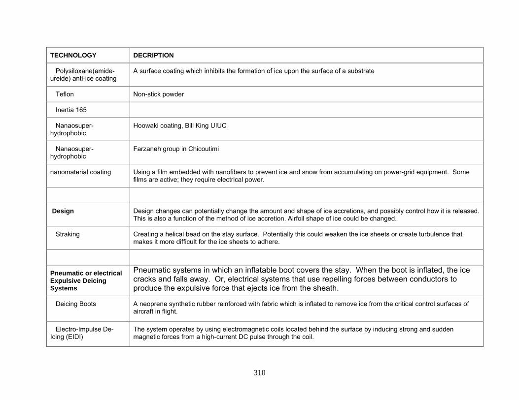
310


Polysiloxane(amide-ureide) anti-ice coating

A surface coating which inhibits the formation of ice upon the surface of a substrate

Teflon Non-stick powder

Inertia 165

Nanaosuper-hydrophobic

Hoowaki coating, Bill King UIUC

Nanaosuper-hydrophobic

Farzaneh group in Chicoutimi

nanomaterial coating Using a film embedded with nanofibers to prevent ice and snow from accumulating on power-grid equipment. Some films are active; they require electrical power.

Design Design changes can potentially change the amount and shape of ice accretions, and possibly control how it is released. This is also a function of the method of ice accretion. Airfoil shape of ice could be changed.

Straking Creating a helical bead on the stay surface. Potentially this could weaken the ice sheets or create turbulence that makes it more difficult for the ice sheets to adhere.

Pneumatic or electrical Expulsive Deicing Systems

Pneumatic systems in which an inflatable boot covers the stay. When the boot is inflated, the ice cracks and falls away. Or, electrical systems that use repelling forces between conductors to produce the expulsive force that ejects ice from the sheath.

Deicing Boots A neoprene synthetic rubber reinforced with fabric which is inflated to remove ice from the critical control surfaces of aircraft in flight.

Electro-Impulse De-Icing (EIDI)

The system operates by using electromagnetic coils located behind the surface by inducing strong and sudden magnetic forces from a high-current DC pulse through the coil.

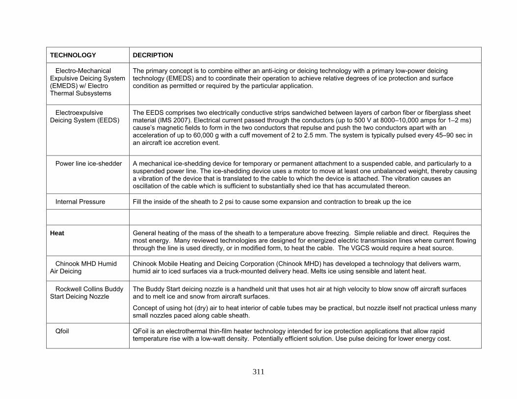
311


Electro-Mechanical Expulsive Deicing System (EMEDS) w/ Electro Thermal Subsystems

The primary concept is to combine either an anti-icing or deicing technology with a primary low-power deicing technology (EMEDS) and to coordinate their operation to achieve relative degrees of ice protection and surface condition as permitted or required by the particular application.

Electroexpulsive Deicing System (EEDS)

The EEDS comprises two electrically conductive strips sandwiched between layers of carbon fiber or fiberglass sheet material (IMS 2007). Electrical current passed through the conductors (up to 500 V at 8000–10,000 amps for 1–2 ms) cause’s magnetic fields to form in the two conductors that repulse and push the two conductors apart with an acceleration of up to 60,000 g with a cuff movement of 2 to 2.5 mm. The system is typically pulsed every 45–90 sec in an aircraft ice accretion event.

Power line ice-shedder A mechanical ice-shedding device for temporary or permanent attachment to a suspended cable, and particularly to a suspended power line. The ice-shedding device uses a motor to move at least one unbalanced weight, thereby causing a vibration of the device that is translated to the cable to which the device is attached. The vibration causes an oscillation of the cable which is sufficient to substantially shed ice that has accumulated thereon.

Internal Pressure Fill the inside of the sheath to 2 psi to cause some expansion and contraction to break up the ice

Heat General heating of the mass of the sheath to a temperature above freezing. Simple reliable and direct. Requires the most energy. Many reviewed technologies are designed for energized electric transmission lines where current flowing through the line is used directly, or in modified form, to heat the cable. The VGCS would require a heat source.

Chinook MHD Humid Air Deicing

Chinook Mobile Heating and Deicing Corporation (Chinook MHD) has developed a technology that delivers warm, humid air to iced surfaces via a truck-mounted delivery head. Melts ice using sensible and latent heat.

Rockwell Collins Buddy Start Deicing Nozzle

The Buddy Start deicing nozzle is a handheld unit that uses hot air at high velocity to blow snow off aircraft surfaces and to melt ice and snow from aircraft surfaces.

Concept of using hot (dry) air to heat interior of cable tubes may be practical, but nozzle itself not practical unless many small nozzles paced along cable sheath.

Qfoil QFoil is an electrothermal thin-film heater technology intended for ice protection applications that allow rapid temperature rise with a low-watt density. Potentially efficient solution. Use pulse deicing for lower energy cost.

312


ThermaWing-Kelly Aerospace Thermal Systems

ThermaWing is a graphite-based thermoelectric heater that protects the leading edge of airfoils.

Potentially efficient solution. Use pulse deicing for lower energy cost.

Low-Power Electrothermal Deicing (LPED)

LPED uses electrical heating elements attached to or installed within a structure requiring ice protection.

Potentially efficient solution. Use pulse deicing for lower energy cost.

Electrical Heat Tracing Heating wires could be installed on the sheath. Partial or complete.

With careful placement may make ice pieces small enough to reduce hazard.

Variable Resistance Cable (VRC) De-icing System

The resistance in a cable is varied to generate heat to melt ice build-up or keep it from forming in the first place. A proprietary technology developed by the Dartmouth Ice Research Lab.

Ice-electrolysis de-icer Variable resistance cable that increases resistance in power lines-to produce heat that melts ice on power lines or prevents new freezing.

Internal hot gas flow The strands occupy roughly 50% of the space within the sheath (See Fig. 1) so hot gases could flow up the inside of the sheath.

Internal electrical heating

It would be possible to pull and electrical resistance cable up inside the stay. Caution: a short circuit could speedup corrosion of the sheath.

Solar Warming System Pave Guard, operates much like radiant heating works in a home’s floor. Tubing is installed in the bridge deck, through which a heated solution is pumped to keep the deck from freezing. The energy to heat the solution is provided by solar panels mounted near the bridge site.

Ecotemp radiant thermal sheet

Heater mat with adhesive backing.

Electrically conductive paint

Battelle Memorial Institute is developing a carbon-nanotube paint. A meeting was held with Battelle to discuss this technology. It has a low commercial readiness level.

Laser deicing Use a laser to remove the ice.

313


Microwave deicing

Radiant Heating Infrared radiant heat sources.

Schaefer Ventilation HotZone Heaters

The HotZone technology consists of a gas or electric infrared source with the energy focused by a unique reflective lens.

Trimac Industrial Systems LLC - Ice-Cat

The Gas-Cat uses a gas-fueled catalytic emitter panel, although electrically powered systems are also available

Radiant Aviation A Radiant Aviation facility consists of an array of energy process units (EPUs), or infrared emitters, mounted on the ceiling of the tension membrane structure. A circular array to move up the stay.

Vacca Inc The Vacca system is a variable output heater that can serve as an infrared emitter.

Interface heating Applying heat directly to the interface between the ice and the stay. This eliminates the need to heat the entire mass of the stay.

Pulse electro-thermal de-icing (PETD) technology

PETD is an electrified coating. The method uses short pulses of electricity applied directly to the ice-substrate interface and, therefore, only has to melt a micrometer-thin layer of ice. . This causes the ice to melt at the interface without heating the entire mass of the stay. The potential for using this system on the VGCS has been discussed with Dr. Petrenko. On the VGCS, the heating would done with short pulses to different areas of the bridge. The system uses about 6kW/m2. On the VGCS, the maximum available power is 600kW. The surface area is 95,000 ft2 (9,000 m2). Thus, the VGCS stays would have to be heated in about 90 100 m2 pieces. The time to de-ice would be roughly 35 minutes. The system has been installed on the Uddevalla Bridge. (Petrenko videos) On this bridge application, batteries were used to give a surge of power. Recently, a roof with a 10,000 m2 area has been coated. PETD was developed by the Dartmouth Ice Research Lab.

High-Velocity Air, Water, or Steam

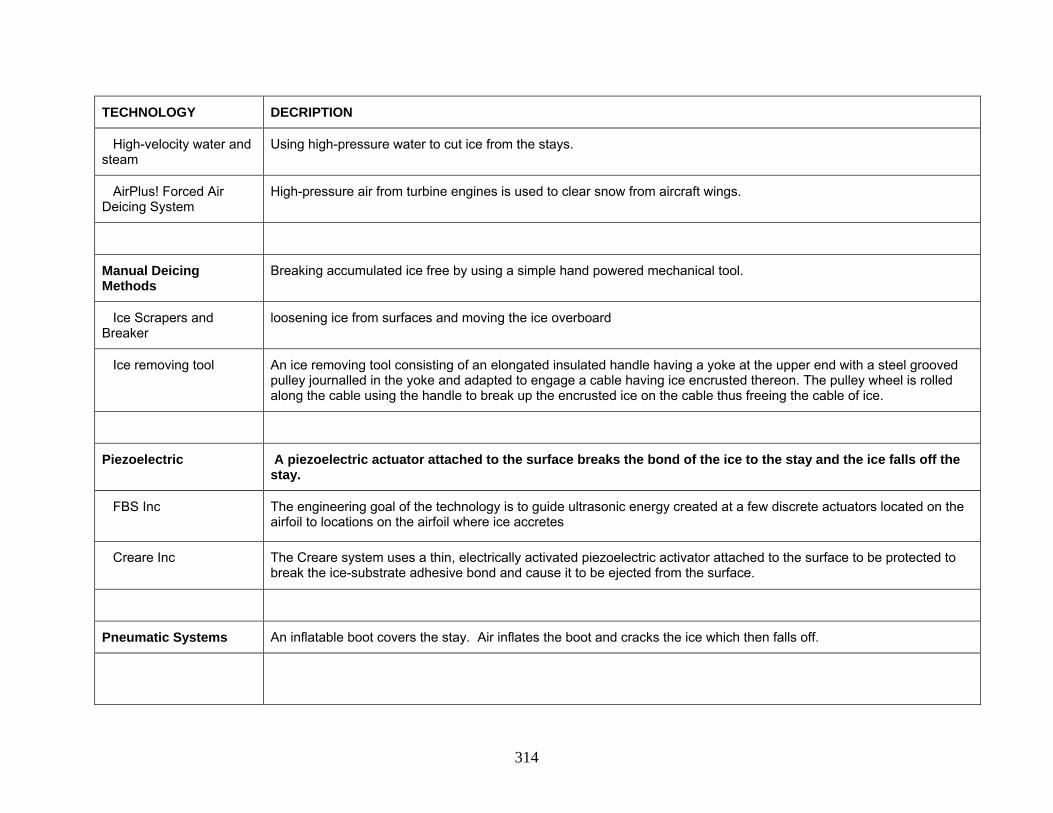
314


High-velocity water and steam

Using high-pressure water to cut ice from the stays.

AirPlus! Forced Air Deicing System

High-pressure air from turbine engines is used to clear snow from aircraft wings.

Manual Deicing Methods

Breaking accumulated ice free by using a simple hand powered mechanical tool.

Ice Scrapers and Breaker

loosening ice from surfaces and moving the ice overboard

Ice removing tool An ice removing tool consisting of an elongated insulated handle having a yoke at the upper end with a steel grooved pulley journalled in the yoke and adapted to engage a cable having ice encrusted thereon. The pulley wheel is rolled along the cable using the handle to break up the encrusted ice on the cable thus freeing the cable of ice.

Piezoelectric A piezoelectric actuator attached to the surface breaks the bond of the ice to the stay and the ice falls off the stay.

FBS Inc The engineering goal of the technology is to guide ultrasonic energy created at a few discrete actuators located on the airfoil to locations on the airfoil where ice accretes

Creare Inc The Creare system uses a thin, electrically activated piezoelectric activator attached to the surface to be protected to break the ice-substrate adhesive bond and cause it to be ejected from the surface.

Pneumatic Systems An inflatable boot covers the stay. Air inflates the boot and cracks the ice which then falls off.

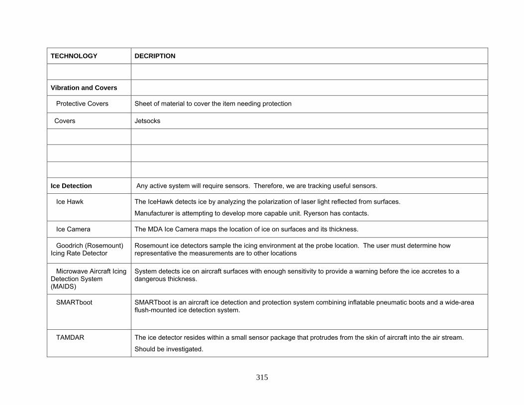
315


Vibration and Covers

Protective Covers Sheet of material to cover the item needing protection

Covers Jetsocks

Ice Detection Any active system will require sensors. Therefore, we are tracking useful sensors.

Ice Hawk The IceHawk detects ice by analyzing the polarization of laser light reflected from surfaces.

Manufacturer is attempting to develop more capable unit. Ryerson has contacts.

Ice Camera The MDA Ice Camera maps the location of ice on surfaces and its thickness.

Goodrich (Rosemount) Icing Rate Detector

Rosemount ice detectors sample the icing environment at the probe location. The user must determine how representative the measurements are to other locations

Microwave Aircraft Icing Detection System (MAIDS)

System detects ice on aircraft surfaces with enough sensitivity to provide a warning before the ice accretes to a dangerous thickness.

SMARTboot SMARTboot is an aircraft ice detection and protection system combining inflatable pneumatic boots and a wide-area flush-mounted ice detection system.

TAMDAR The ice detector resides within a small sensor package that protrudes from the skin of aircraft into the air stream.

Should be investigated.

316


Vaisala The in situ DRS511 sensor (Figure 102) detects roadway surface conditions by making six measurements.

Visidyne first non-contact sensing system for detecting the accumulation of ice on rotorcraft blades in flight

Pole-Ice represent ice accumulation on electrical transmission lines

Supporting Equipment Technology that can be used in conjunction with a primary technology for anti/deicing.

Robotic Climber Some type of robotic device that can climb up the stays to apply a coating or scrap off the ice in a manner that the size of the particles are of a desired size

134489_FR

Documents

Transcript of 134489_FR