12 DETERMINING THE SATURATED HYDRAULIC CONDUCTIVITY

R.J. Oosterbaan and H.J. Nijland

On web site https://ww.waterlog.info public domain, latest upload 20-11-2017

Chapter 12 in: H.P.Ritzema (Ed.), Drainage Principles and Applications. International

Institute for Land Reclamation and Improvement ( ILRI), Publication 16, second revised

edition, 1994, Wageningen, The Netherlands. ISBN 90 70754 3 39

Table of contents

12 DETERMINING THE SATURATED HYDRAULIC............................................................................. 1

12.1 Introduction ................................................................................................................................................ 1

12.2 Definitions.................................................................................................................................................. 1

12.3 Variability of hydraulic conductivity ......................................................................................................... 2

12.3.1. Introduction ................................................................................................................................ 2 12.3.2 Variability within soil layers .............................................................................................................. 3 12.3.3. Variability between soil layers .......................................................................................................... 4 12.3.4. Seasonal variability and time trend.................................................................................................... 4 12.3.5. Soil salinity, sodicity, and acidity...................................................................................................... 5 12.3.6. Geo-morphology................................................................................................................................ 5

12.4 Drainage conditions and hydraulic conductivity ........................................................................................ 6

12.4.1. Introduction ....................................................................................................................................... 6 12.4.2. Unconfined aquifers .......................................................................................................................... 6 12.4.3. Semi-confined aquifers...................................................................................................................... 9 12.4.4. Land slope ....................................................................................................................................... 11 12.4.5. Effective soil depth.......................................................................................................................... 12

12.5 Review of the methods of determination.................................................................................................. 15

12.5.1. Introduction ..................................................................................................................................... 15 12.5.2. Correlation methods ........................................................................................................................ 16 12.5.3. Hydraulic laboratory methods ......................................................................................................... 17 12.5.4. Small-scale in-situ methods ............................................................................................................. 17 12.5.5. Large-scale in-situ methods ............................................................................................................. 19

12.6. Examples of small-scale in-situ methods ................................................................................................ 20

12.6.1. The auger-hole method .................................................................................................................... 20 12.6.2. Inversed auger-hole method ............................................................................................................ 24

12.7. Examples of methods using parallel drains ............................................................................................. 28

12.7.1. Introduction ..................................................................................................................................... 28 12.7.2. Procedures of analysis ..................................................................................................................... 29 12.7.3. Drains with entrance resistance, deep soil ....................................................................................... 32 12.7.4. Drains with entrance resistance, shallow soil .................................................................................. 33 12.7.5. Ideal drains, medium soil depth....................................................................................................... 35

References ........................................................................................................................................................ 37

1

12 DETERMINING THE SATURATED HYDRAULIC R.J. Oosterbaan and H.J. Nijland 12.1 Introduction The design and functioning of subsurface drainage systems depends to a great extent on the soil's saturated hydraulic conductivity (K). All drain- spacing equations make use of this parameter. To design or evaluate a drainage project, we therefore have to determine the K-value as accurately as possible. The K-value is subject to variation in space and time (Section 12.3), which means that we must adequately assess a representative value. This is time-consuming and costly, so a balance has to be struck between budget limitations and desired accuracy. As yet, no optimum surveying technique exists. Much depends on the skill of the surveyor. To find a representative K-value, the surveyor must have a knowledge of the theoretical relationships between the envisaged drainage system and the drainage conditions in the survey area. This will be discussed in Section 12.4. Various methods have been developed to determine the K-value of soils. The methods are categorized and briefly described in Section 12.5, which also summarizes the merits and limitations of each method. Which method to select for the survey of K depends on the practical applicability, and the choice is limited. Two widely used small-scale in-situ methods are presented in Section 12.6. Because of the variability of the soil's K-value, it is better to determine it from large-scale experiments (e.g. from the functioning of existing drainage systems or from drainage experimental fields), rather than from small-scale experiments. Section 12.7 presents examples of some of the more common flow conditions in large-scale experiments. 12.2 Definitions The soil's hydraulic conductivity was defined in Chapter 7 as the constant of proportionality in Darcy's Law V = K dh/dx (12.1) where V = apparent velocity of the groundwater (m/d) K = hydraulic conductivity (m/d) h = hydraulic head (m) x = distance in the direction of groundwater flow (m) In Darcy's Equation, dh/dx represents the hydraulic gradient (s), which is the difference of h over a small difference of x. Hence, the hydraulic conductivity can be expressed as K = V/s and can thus be regarded as the apparent velocity (m/d) of the groundwater when the hydraulic gradient equals unity (s = 1). In practice, the value of the hydraulic gradient is generally less than 0.1, so that v is usually less than 0.1K. Since the value of K is also usually less than 10 m/d, it follows that v is almost always less than 1 m/d. The K-value of a saturated soil represents its average hydraulic conductivity, which depends mainly on the size, shape, and distribution of the pores. It also depends on the soil temperature and the viscosity and density of the water. These aspects were discussed in Chapter 7. In some soils (e.g. unstructured sandy sediments), the hydraulic conductivity is the same in all directions. Usually, however, the value of K varies with the direction of flow. The vertical permeability of the soil or of a soil layer is often different from its horizontal permeability because of vertical differences in texture, structure, and porosity due to a layered deposition or horizon development and biological activity. A soil in which the hydraulic conductivity is direction-dependent is an-isotropic (Chapter 3). Anisotropy plays an important role in land drainage, because the flow of groundwater to the drains can, along its flow path, change from vertical to horizontal and intermediate between them (Chapter 8). The hydraulic conductivity in horizontal direction is indicated by Kh, in vertical direction by Kv, and in an intermediate direction, especially in the case of radial flow to a drain, by Kr. The value of Kr for radial flow is often computed from the geometric, or logarithmic, mean of Kh and Kv (Boumans 1976):

2

Kr = √(Kh Kv) (12.3) or log = 0.5 (log Kh + log Kv ) (12.4) Examples of Kh and Kv values determined in core samples are shown in Figure 12.1.

Kh = 5.0 5.5 8.1 5.0 Kv = 2.5 0.9 8.2 1.4 Figure 12.1 Core samples from laminated tidal flat deposits with different K-values (m/d) in horizontal (Kh) and vertical (Kv) direction (Wit 1967) 12.3 Variability of hydraulic conductivity

12.3.1. Introduction The K-value of a soil profile can be highly variable from place to place, and will also vary at different depths (spatial variability). Not only can different soil layers have different hydraulic conductivities (Section 12.3.3), but, even within a soil layer, the hydraulic conductivity can vary (Section 12.3.2). In alluvial soils (e.g. in river deltas and valleys), impermeable layers do not usually occur at shallow depth (i.e. within 1 or 2 m). In subsurface drainage systems in alluvial soils, not only the K-values at drain depth are important, but also the K-values of the deeper soil layers. This will be further discussed in Section 12.4. Soils with layers of low hydraulic conductivity or with impermeable layers at shallow depth are mostly associated with heavy, montmorillonitic or smectitic clay (vertisols), with illuviated clay in the sandy or silty layer at 0.5 to 0.8 m depth (Planosols), or with an impermeable bedrock at shallow depth (Chapter 3). Vertisols are characterized by a gradually decreasing K-value with depth because the topsoil is made more permeable by physical and biological processes, whereas the subsoil is not. Moreover, these soils are subject to swelling and shrinking upon wetting and drying, so that their K-value is also variable with the season, being smaller during the humid periods when drainage is required. If subsurface drains are to be installed, the K-values must be measured during the humid period. Seasonal variability studies are therefore important (Section 2.3.4). If subsurface drainage of these soils is to be cost-effective, the drains must be installed at shallow depth (< 1 m). Planosols can occur in tropical climates with high seasonal rainfalls. Under such conditions, a high drainage capacity is required and, if the impermeable layer is shallower than approximately 0.8 m, the cost-effectiveness of subsurface drainage becomes doubtful.

3

Soil salinity, sodicity, and acidity also have a bearing on the hydraulic conductivity (Section 12.3.5). The variations in hydraulic conductivity and their relationship with the geomorphology of an area are discussed in Section 12.3.6.

12.3.2 Variability within soil layers Measured K-values of a soil often show a log-normal distribution with a wide variation (Dieleman and Trafford 1976). Figure 12.2 shows a plot of the logarithm of K-values against the cumulative frequency on normal probability paper. The data were collected with the auger-hole method in an area of about 100 ha in a coastal valley of Peru, which has sandy loam soils and a water table at a depth of about 2 m. The figure shows that, except for the two highest and lowest observations, the data obey the log-normal distribution.

1 5 25 50 75 95 99

-1.0

-0.8

-0.6

-0.4

-0.2

0

0.2

0.4

log K K in m / d

0.1

0.2

0.3

0.4

0.6

1.0

1.6

2.5

cumulat ive frequency in % Figure 12.2 The cumulative normal frequency distribution of K-values measured according to the auger-

hole method in an area of 100 ha in a coastal valley of Peru A representative value of K may be found from the geometric mean n K* = √(K1 x K2 x … x Kn) (12.5) where n is the total number of observations Taking the log value of K* we find from Equation 12.5 that Log K* = (log K1 + log K1 + … + log K1)/n (12.6) From this equation, we can see that log K* is the arithmetic mean of the log K-values. This corresponds to the mean value of the log-normal distribution (Chapter 6). The K-values in Figure 12.2 range from 0.1 to 2.5 m/d and have a standard deviation of 0.6 m/d. The arithmetic mean is 0.8 m/d, and the modal and median values, as well as the geometric mean, are 0.6 m/d. This illustrates the characteristic that, in a log-normal distribution, the geometric mean, the mode, and the median are the same and that these values correspond to the mode and median of the original distribution of the K-values (i.e. without taking their logarithms). The representative K-value of a soil layer can therefore be found simply as the modal or the median value of the frequency distribution of the observed K-values without log-transformation. Bouwer and Jackson (1974) conducted electric model tests with randomly distributed electric resistances to represent randomly varied K-values, and found that the geometric mean gave the most representative value.

4

Bentley et al. (1989), however, using the finite element method to determine the effect of the variation in K-values on the draw down of the water table between drains, concluded that the best estimate would be the average of the arithmetic mean and the geometric mean. The standard deviation of the observed K-values depends on the method of determination. This will be discussed in Section 12.6.

12.3.3. Variability between soil layers When a soil shows a distinct layering, it is often found that the representative K-values of the layers differ. Generally, the more clayey layers have a lower K-value than the more sandy layers, but this is not always true (Section 12.6.2). The representative value of K in layered soils depends on the direction of flow of the groundwater. When the water flows parallel to the soil layers, the representative value is based on a summation of the hydraulic transmissivities of the layers, but, when the water flows perpendicular to the layers, one uses a summation of the hydraulic resistances of the layers. This was explained in Chapter 7, and the results are summarized below. The total transmissivity of soil layers for flow in the direction of the layers is calculated as n K*Dt = Σ KiDi (12.7) i=1 where K* = weighted average K-value of the soil layers (m/d) Dt = total thickness of the soil layers (m) i = number of the soil layer The value KiDi represents the hydraulic transmissivity for flow (m2/d) of the i-th soil layer. It can be seen from Equation 12.7 that the hydraulic transmissivities of soil layers are additive when the flow occurs in the direction of the layers. It is also seen that, with such flow, the representative value K* of soil layers can be calculated as a weighted mean of the K-values, with the thickness D used as the weighting factor. Using the same symbols as Equation 12.7, we can calculate the total resistance of soil layers to vertical flow as n Dt/K* = Σ Di/Ki (12.8) i=1 where the value D/K represents the hydraulic resistance (c) to vertical flow (Chapter 2). It can be seen from Equation 12.8 that, when the flow occurs perpendicular to the layers, the hydraulic resistances of soil layers are additive. Comparing Equations 12.7 and 12.8, we can readily verify that the K*-value for horizontal flow in soil layers is determined mainly by the layers with the highest K-values, whereas the K*-value for vertical flow in horizontal layers is mainly determined by the layers with the lowest K-values, provided that the soil layers are not too thin.

12.3.4. Seasonal variability and time trend The K-values of the topsoil are often subject to changes with time, which can be seasonal variations or time trends. This is due to the drying of the topsoil during a dry season or after the introduction of drainage. The K- values of the subsoil are less time-variable, because they are less subject to drying and wetting, and biological processes are also less pronounced. The seasonal variability occurs mainly in clay soils with swelling and shrinking properties. Those soils often contain large fractions of montmorillonitic or smectitic clay minerals. Their swelling or shrinking then follows the periodicity of the wet and dry seasons.

5

The time trend may be observed in soils with a high clay or organic fraction. This is due to long-term changes in soil structure and porosity, which depend to a great extent on the prevailing soil-water conditions and are closely related to subsidence (Chapter 13). When drained, these soils are on the average drier than before, which affects their biological conditions or leads to the decay of organic material. Clay soils often show an increased K-value when drained (e.g. van Hoorn 1958; Kuntze 1964; El-Mowelhi and van Schilfgaarde 1982) because of increased biological activity, originating from an improved soil structure. The increase can be dramatic when the soils are reclaimed un-ripened marine sediments. In the Yssel Lake polders of The Netherlands, the K-value of the soil was found to increase from almost zero at the time the new polders were just falling dry, to more than 10 m/d several years after the installation of subsurface drains. Soils with organic material, on the other hand, may show a decreased K-value because of the loss of the organic material that is responsible for their structural stability.

12.3.5. Soil salinity, sodicity, and acidity Soil salinity usually has a positive influence on the hydraulic conductivity, especially in clay soils. Upon reclamation, saline soils may become less permeable. (The process of soil salinization and reclamation techniques will be treated in Chapter 15.) Sodic soils, on the other hand, experience a dispersion of soil particles and a deterioration in the structure, resulting in poor K-values. Sodic soils are formed when sodium-carbonates are present in the soil or are introduced with the irrigation water (Ayers and Westcott 1985). The deteriorating effect of sodium is most pronounced in the top layers of non-saline clay soils with expandable clay minerals such as montmorillonites and smectites (Richards 1954). Careless agricultural practices on such top layers, or overgrazing on them, worsens the situation (Abrol et al. 1988). Sodification and the reclamation of sodic soils will be further discussed in Chapter 15. Acid soils are usually associated with high K-values. The top layers of Latosols, for example, formed by excessive leaching, as happens in the high-rainfall tropical zones, have lost many of their clay and silt particles and their base ions, so that an acid, infertile, sandy soil with a low base saturation remains. Older acid sulphate soils, which developed upon the reclamation of coastal mangrove plains, are also reported to have a good structural stability and high K-values (Scheltema and Boons 1973).

12.3.6. Geo-morphology In flood plains, the coarser soil particles (sand and silt) are deposited as levees near the river banks, whereas the finer particles (silt and clay) are deposited in the back swamps further away from the river. The levee soils usually have a fairly high K-value (from 2 to 5 m/d), whereas the basin soils have low K-values (from 0.1 to 0.5 m/d). Riverbeds often change their course, however, so that the pattern of levee and basin soils in alluvial plains is often quite intricate. In addition, in many basin soils, one finds organic material at various depths, which may considerably increase their otherwise low K-value. The relationship between K-value and geo-morphological characteristics is therefore not always clear.

6

12.4 Drainage conditions and hydraulic conductivity

12.4.1. Introduction To determine a representative value of K, the surveyor must have a theoretical knowledge of the relationships between the kind of drainage system envisaged and the drainage conditions prevailing in the survey area. For example, the surveyor must have some idea of the relationship between the effectiveness of drainage and such features as: - The drain depth and the K-value at this depth; - The depth of groundwater flow and the type of aquifer; - The variation in the hydraulic conductivity with depth; - The anisotropy of the soil. Aquifers are classified according to their relative permeability and the position of the water table (Chapter 2). The properties of unconfined and semi-confined aquifers will be discussed in the following sections.

12.4.2. Unconfined aquifers Unconfined aquifers are associated with the presence of a free water table, so the groundwater can flow in any direction: horizontal, vertical, and/or intermediate between them. Although the K-values may vary with depth, the variation is not so large and systematic that specific layers need or can be differentiated. For drainage purposes, unconfined aquifers can be divided into shallow aquifers, aquifers of intermediate depth, and deep aquifers. Shallow unconfined aquifers have a shallow impermeable layer (say at 0.5 to 2 m below the soil surface). Intermediate unconfined aquifers have impermeable layers at depths of, say, from 2 to 10 m below the soil surface. Deep unconfined aquifers have their impermeable layer at depths ranging from 10 to 100 m or more. Shallow Unconfined Aquifers

The flow of groundwater to subsurface drains above a shallow impermeable layer is mainly horizontal and occurs mostly above drain level (Figure 12.3). In shallow unconfined aquifers, it usually suffices to measure the horizontal hydraulic conductivity of the soil above drain level (i.e. Ka). The recharge of water to a shallow aquifer occurs only as the percolation of rain or irrigation water; there is no upward seepage of groundwater nor any natural drainage. Since the transmissivity of a shallow aquifer is small, the horizontal flow in the absence of subsurface drains is usually negligible.

ditch orpipedrain

water divide

impermeable layer

water table

mainly horizontal f low

Figure 12.3 Flow of groundwater to subsurface drains in shallow unconfined aquifers

7

Unconfined Aquifers of Intermediate Depth The flow of groundwater to subsurface drains in unconfined aquifers of intermediate depth is partly horizontal and partly radial (Figure 12.4). For such aquifers, it is important to know the horizontal hydraulic conductivity above and below drain level (i.e. Ka and Kb), as well as the hydraulic conductivity (Kr) in a radial direction to the drains, below drain level (Chapter 8). Although there is also vertical flow, the corresponding hydraulic resistance is mostly small and need not be taken into account. In similarity to the shallow unconfined aquifer, the recharge of water to an unconfined aquifer of intermediate depth consists mainly of the downward percolation of rain or irrigation water. Here, too, little upward seepage or natural drainage of groundwater occurs, and the horizontal flow in the absence of subsurface drains is negligibly small compared to the vertical flow.

ditch or

pipedrain

soil surface

water divide

impermeable layer

radialf low

mainly horizontal f low

water table

Figure 12.4 Flow of groundwater to subsurface drains in unconfined aquifers of intermediate depth Deep Unconfined Aquifers

The groundwater flow to subsurface drains in deep unconfined aquifers is mainly radial towards the drains, and the hydraulic resistance takes place mainly below drain level. To determine the hydraulic conductivity for radial flow, we therefore have to know the horizontal (Kh) and the vertical hydraulic conductivity (Kv) of the soil below drain depth (See Equations 12.3 and 12.4). The recharge consists of deep percolation from rain or irrigation, but at the same time there may be upward seepage of groundwater or natural drainage (Figure 12.5).

8

soil surface

soil surface

soil surface

A

B

C

water divide

ditch orpipedrain

ditch orpipedrain

ditch orpipedrain

wa abter t lepercolat ion

deep flow ofpercolat ion water

percolat ion

percolat ion

wat a ler t b e

wat a ler t b e

upwardseepage

flow depth of percolat ionwater rest r icted due to

upward seepage

natural drainageto the aquifer

Figure 12.5 Flow of groundwater to subsurface drains in deep unconfined aquifers; A: No seepage and natural drainage; B: Seepage; C: Natural drainage The seepage or natural drainage depends on the transmissivity of the aquifer and the geohydrological conditions (Chapter 9). For example, in sloping lands, there are often higher-lying regions where the natural drainage dominates and lower-lying regions where the seepage prevails, provided that the transmissivity of the aquifer is high enough to permit the horizontal transport of a considerable amount of groundwater over long distances (Figure 12.6).

9

Figure 12.6 A deep unconfined aquifer with groundwater flow from a percolation zone towards a seepage zone When there is no upward seepage or natural drainage in deep unconfined aquifers, the depth to which the percolation water descends, before ascending again to subsurface drains, is limited, because otherwise the resis-tance to vertical flow becomes too large. When the soil is homogeneous and permeable to a great depth, the main part of drainage flow extends to depths of 0.15L to 0.25L (where L is the drain spacing) beneath the drain level. In most soils, however, the flow below drain level is limited by poorly permeable layers and/or by the anisotropy of the substrata, which is common in most alluvial soils (Smedema and Rycroft 1983). Hence, it is not necessary to determine the K-values at a depth greater than 10% of the drain spacing. This will be further discussed in Section 12.4.5. When upward seepage of groundwater occurs, the depth to which the percolation water penetrates before ascending to the drains is further reduced (Figure 12.5B), but at the same time the seepage water comes from great depths. The percolation and seepage water join to continue as radial flow to the drains. The maximum depth for which K-values need to be known therefore corresponds to the same 10% of the drain spacing as mentioned above. When, on the other hand, natural drainage to the underground occurs, not all of the percolating water will reach the drains. The zone of influence of the drains no longer equals half the drain spacing, but is less than that (Figure 12.5C). The maximum depth over which one needs to know the K-values is therefore less than 10% of the drain spacing. If the natural drainage is great enough, no artificial drainage is required at all, and no survey of K-values needs to be made. An important characteristic of deep unconfined aquifers is that, when the water table is lowered by a subsurface drainage system, this does not appreciably increase the seepage or reduce the natural drainage, unless a subsurface drainage system is installed in isolated small areas (Chapter 16). This is in contrast to the characteristics of semi-confined aquifers as will be discussed below.

12.4.3. Semi-confined aquifers Semi-confined aquifers are characterized by the presence of a pronounced layer with relatively low K-values (i.e. the aquitard) overlying the aquifer. Without drains, the water flow in the aquitard is mainly vertical. Semi-confined aquifers are common in river deltas and coastal plains, where slowly permeable clay soils overlie highly permeable sandy or even gravelly soils. Because of its relatively low K-value, the aquitard limits seepage from the aquifer, but at the same time it can maintain a large difference between the water table in the aquitard and the piezometric level in the aquifer. Hence, if the aquitard is made more permeable by a drainage system and the water table is lowered, the flow of water from aquifer into aquitard may increase considerably. This occurs especially when the aquitard is not very deep (say 2 to 3 m), and mainly in those parts of the drainage system situated at the upstream end of the aquifer. As a consequence of the increased seepage at the upstream end, the discharge of the aquifer at the downstream end is often reduced, compared with the situation before drainage (Figure 12.7).

10

soil surface

aquifer

aquitard

subsurface drainage systemsoi l surface

aquifer

aquitard

A

B

original water table

water table with drainage

water table

f low lines

f low l

ines

Figure 12.7 A semi-confined aquifer with groundwater flow; A: Before drainage, and B: After drainage, showing an interception effect In other words, the upstream drains have intercepted part of the aquifer discharge; they have lowered the water table in the aquifer downstream, and have reduced the seepage downstream. If we know the transmissivity of the aquifer and the hydraulic resistance of the aquitard, we can calculate the amount of intercepted groundwater. (Methods to determine these hydraulic characteristics were presented in Chapter 10.) The aquitard may reach the soil surface, or remain below it (Figure 12.8). If the aquitard is below the soil surface, the semi-confined aquifer is more complex because there is an unconfined aquifer above it. (The unconfined aquifer in Figure 12.8 is sometimes called a "leaky aquifer".) In this case, subsurface drainage should rather be seen as drainage of an unconfined aquifer, whereby the horizontal conductivity of the aquitard is taken as Kh = 0, but the vertical conductivity as Kv > 0. As a consequence, the drainage conditions discussed in Section 12.4.2 remain applicable, except that a lowering of the water table by subsurface drainage may possibly increase the upward seepage of groundwater (Figure 12.8A).

11

piezometric level

seepage

A B

aquiclude aquiclude

aquitard aquitard

naturaldrainage

unconfined aquiferunconfined aquifer

semi-confined aquifer semi-confined aquifer

piezometric level

water table water table

Figure 12.8 Semi-confined aquifer overlain by an unconfined aquifer; A: Seepage; B: Natural drainage A semi-confined aquifer need not always have overpressure and seepage. In the southern part of the Nile Delta, for example, the piezometric level in the semi-confined aquifer is below the water table in the aquitard (Figure 12.8B), which indicates the presence of natural drainage instead of upward seepage (Amer and de Ridder 1989). In such cases, the zone of influence of subsurface drains is less than half the drain spacing and the flow of percolation water to the drains, if occurring at all, reaches less deep. Consequently, the K-value need not be surveyed at great depth, unless the drainage project is associated with the introduction of irrigation, which will involve the supply of considerable amounts of water and which will change the hydrological conditions.

12.4.4. Land slope If the drained land has a certain slope, the zone of influence in upslope direction is greater than half the drain spacing, whereas in downstream direction it is less (Figure 12.9). In deep unconfined aquifers, this results in a deeper flow of the groundwater to the drains at their upstream side compared with the situation of zero slope, whereas at the downstream side the reverse is true (Oosterbaan and Ritzema 1992). In sloping lands, therefore, we have to know the value of K to a greater depth than in flat land.

12

soil sur

face

water divide

water table

Figure 12.9 Subsurface drainage of a deep unconfined aquifer in sloping land

12.4.5. Effective soil depth In a system of subsurface drains, the effective soil depth over which the K-value should be known depends on the depth of the impermeable layer and the sequence of the layers with higher and lower K-values, as was illustrated in the previous sections. In the following sections, examples are given to clarify the concept of the effective soil depth a little further. Example 12.1 The Effective Soil Depth of a Homogeneous Deep Unconfined Aquifer

Figure 12.10 presents the pattern of equipotential lines and streamlines in a deep homogeneous soil to a field drain, for two different cases. As was discussed in Chapter 7, each square in a flow-net diagram represents the same amount of flow. By counting the number of squares above and below a certain depth, we can estimate the percentage of flow occurring at a certain moment above and below that depth. The result of the counting is given in Table 12.1.

-4

-3

-2

-1

0

1

2

-4

-3

-2

-1

0

1

2

0

streamline

1 2 3 4 5 0 1 2 3 4 5

distance in m

height above drainlevel in m

equipotential

water table

percolation

water table

Figure 12.10 Equipotentials and streamlines of groundwater flow to drains in deep homogeneous soils (Childs 1943)

13

Table 12.1 Count of squares in Figure 12.10 ------------------------------------------------------------------------------------ Depth (z) below drain level Number of squares above z in % in % of spacing --------------------------------------- Figure 12.10A Figure 12.10B ------------------------------------------------------------------------------------ 5 74 76 10 88 87 15 94 93 25 98 97 ------------------------------------------------------------------------------------ Table 12.1 shows that 75% of the total flow at a certain time occurs above a depth z = 0.05L, where L is the drain spacing. In shallower soils, this fraction will even be more. So, for spacing of L = 10 m, by far the greater part of the total flow is found above a depth of 0.5 m below drain level and, for spacing of L = 100 m, this depth is still only 5 m. From this analysis, we can deduce that the hydraulic conductivity of the soil layers just above and below drain level is of paramount importance. This explains why, in deep homogeneous soils, K-values determined with experimental drains are quite representative for different drain depths and spacing. In layered soils, the effective depth is different from that described in Example 12.1 for homogeneous soils. This will be illustrated in Example 12.2. Example 12.2 Influence of the Hydraulic Conductivity of the Lower Soil Layer on the Hydraulic Head

between the Drains

Consider three soil profiles with an upper soil layer of equal thickness (D1 = 2 m) and a deep lower soil layer (D2 ≥ 10 m). The hydraulic conductivity of the upper layer is fixed (Kt = 1 m/d), whereas the hydraulic conductivity of the deeper layer varies (Figure 12.11). We can calculate the hydraulic head between the drains using the appropriate drainage equation (Chapter 8), with drain spacing L = 50 m, drain radius ro = 0.10 m, and drain discharge q = 0.005 m/d. The results are given in Table 12.2. Table 12.2 Calculations of h for three soil profiles with data from Example 12.2 ---------------------------------------------------------------------------------------------------------- Hydraulic Drainage equation Hydraulic Situation conductivity (Chapter 8) head h (m) Kb (m/day) ---------------------------------------------------------------------------------------------------------- A 0.1 Hooghoudt, lower soil layer is impermeable base, 0.75 equivalent depth d = 1.71 m B 1 Hooghoudt, K = K1 = Kb 0.40 D > 12 m and d = 3.74 m C 10 Ernst, Dh = 10 m, Dr = 2 m 0.28 u = 0.1π m and a = 4.2 ---------------------------------------------------------------------------------------------------------- It can be seen from Table 12.2 that, if the hydraulic conductivity of the deeper soil layer is markedly different from that of the upper soil layer, the K-value of the deeper soil layer exerts a considerable influence on the hydraulic head. If, instead of taking constant drain spacing, we had taken the hydraulic head as constant, we would similarly find a considerable influence on the spacing. These two examples show that, if one has knowledge of the functioning of the drainage system in relation to the aquifer conditions, this can contribute greatly to the formulation of an effective program for determining a representative K-value.

14

soil surface

soil surface

soil surface

h= 0.75 m

h= 0.40 m

h= 0.25 m

D = 2.00 m1

D = 2.00 m1

D= D

+ D

> 12.00 m

12

D = 2.00 m1

D > 10.00 m2

D > 10.00 m2

D > 10.00 m2

A

B

C

impermeable layer

K = K = 1 m/ d1

K = 1 m/ d

K = 1 m/ d

K = 10 m/ d

K = 0.1 m/ d

t

b

K = 1 m/ d

t

b

impermeable layer

t

b

impermeable layer

Figure 12.11 Drainage cases with different soil profiles (Example 12.2)

15

12.5 Review of the methods of determination

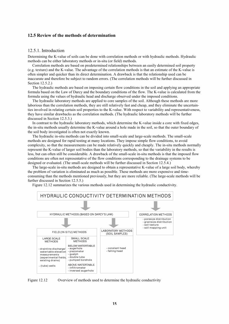
12.5.1. Introduction Determining the K-value of soils can be done with correlation methods or with hydraulic methods. Hydraulic methods can be either laboratory methods or in-situ (or field) methods. Correlation methods are based on predetermined relationships between an easily determined soil property (e.g. texture) and the K-value. The advantage of the correlation methods is that an estimate of the K-value is often simpler and quicker than its direct determination. A drawback is that the relationship used can be inaccurate and therefore be subject to random errors. (The correlation methods will be further discussed in Section 12.5.2.) The hydraulic methods are based on imposing certain flow conditions in the soil and applying an appropriate formula based on the Law of Darcy and the boundary conditions of the flow. The K-value is calculated from the formula using the values of hydraulic head and discharge observed under the imposed conditions. The hydraulic laboratory methods are applied to core samples of the soil. Although these methods are more laborious than the correlation methods, they are still relatively fast and cheap, and they eliminate the uncertain-ties involved in relating certain soil properties to the K-value. With respect to variability and representativeness, they have similar drawbacks as the correlation methods. (The hydraulic laboratory methods will be further discussed in Section 12.5.3.) In contrast to the hydraulic laboratory methods, which determine the K-value inside a core with fixed edges, the in-situ methods usually determine the K-value around a hole made in the soil, so that the outer boundary of the soil body investigated is often not exactly known. The hydraulic in-situ methods can be divided into small-scale and large-scale methods. The small-scale methods are designed for rapid testing at many locations. They impose simple flow conditions, to avoid complexity, so that the measurements can be made relatively quickly and cheaply. The in-situ methods normally represent the K-value of larger soil bodies than the laboratory methods, so that the variability in the results is less, but can often still be considerable. A drawback of the small-scale in-situ methods is that the imposed flow conditions are often not representative of the flow conditions corresponding to the drainage systems to be designed or evaluated. (The small-scale methods will be further discussed in Section 12.5.4.) The large-scale in-situ methods are designed to obtain a representative K-value of a large soil body, whereby the problem of variation is eliminated as much as possible. These methods are more expensive and time- consuming than the methods mentioned previously, but they are more reliable. (The large-scale methods will be further discussed in Section 12.5.5.) Figure 12.12 summarizes the various methods used in determining the hydraulic conductivity.

- poresize dist ribut ion- grainsize dist ribut ion- soil texture- soil mapping unit

LARGE SCALEMETHODS

drainl ine discharge/water table elevat ionmeasurements(experimental fields,exist ing drains)

(tube) wells

SMALL SCALEMETHODS

BELOW WATERTABLE- augerhole- piezometer- guelph- double tube- pumped borehole

ABOVE WATERTABLE- infi lt rometer- inversed augerhole

- constant head- fal l ing head

-

-

Figure 12.12 Overview of methods used to determine the hydraulic conductivity

16

12.5.2. Correlation methods The correlation methods for determining K-values in drainage surveys are frequently based on relationships between the K-value and one or more of the following soil properties: texture, pore-size distribution, grain-size distribution, or with the soil mapping unit. Details of soil properties were given in Chapter 3. Soil Texture

Soil texture refers to the percentage of sand, silt, and clay particles in the soil. Texture or textural class is often used for the correlation of K- values with other hydraulic properties of the soil (e.g. water-holding capacity and drainable pore space) (Wösten, 1990). Aronovici (1947) presented a correlation between the content of silt and clay of subsoil materials in the Imperial Valley in California, U.S.A., and the results of hydraulic laboratory tests. Smedema and Rycroft (1983) give generalized tables with ranges of K-values for certain soil textures (Table 12.3). Such tables (See also Chapter 7, Table 7.2), however, should be handled with care. Smedema and Rycroft warn that: "Soils with identical texture may have quite different K-values due to differences in structure" and "Some heavy clay soils have well-developed structures and much higher K-values than those indicated in the table". Table 12.3 Range of K-values by soil texture (Smedema and Rycroft 1983) Texture K (m/day) Gravelly course sand 10 - 50 Medium sand 1 - 5 Sandy loam, fine sand 1 - 3 Loam, well structured clay loam and clay 0.5 - 2 Very fine sandy loam 0.2 - 0.5 Poorly structured clay loam and clay 0.002 - 0.2 Dense clay (no cracks, no pores) < 0.002 Pore-Size Distribution of the Soil

The pore-size distribution, the regularity of the pores, and their continuity has a great influence on the soil's K-values. Nevertheless, the study and characterization of the porosity aiming at an assessment of the K-values is not sufficiently advanced to be practical on a large scale. An example of the complexity of such a study using micromorphometric data is given by Bouma et al. (1979) for clay soils. Another example is given by Marshall (1957), who determined the pore-size distribution using the relationship between soil-water content and matric head (Chapter 3). Applying Poiseuille's Law to a number of fractions of the pF-curve, he was able to calculate the K-value. Marshall's method is mainly applicable to granular (sandy) soils having no systematic continuous pores. Grain-Size Distribution of the Soil

In sandy soils, which have no systematic continuous pores, the soil permeability is related to the grain-size distribution. Determining the K- value from the grain-size distribution uses the specific surface ratio (U) of the various grain-size classes. This U-ratio is defined as the total surface area of the soil particles per unit mass of soil, divided by the total surface area of a unit soil mass consisting of spherical particles of 1 cm diameter. The U-ratio, the porosity, and a shape factor for the particles and the voids allow us to calculate the hydraulic conductivity. This method is seldom used in land drainage practice because the homogeneous, isotropic, purely-granular soils to which it applies are rare. An example of its use for deep aquifers is given in de Ridder and Wit (1965).

17

Soil Mapping Unit

In the U.S.A., soil mapping is often done on the basis of soil series, in which various soil properties are combined, and these series are often correlated to a certain range of K-values. For example, Camp (1977) measured K-values of a soil series called Commerce silt loam and he reports that the K-values obtained with the auger-hole method were in the range of 0.41 to 1.65 m/d, which agreed with the published K-values for this soil. Anderson and Cassel (1986) performed a survey of K-values of the Portsmouth sandy loam, using core samples. They found a very large variation of more than 100%, which indicates that the correlation with soil series is difficult.

12.5.3. Hydraulic laboratory methods Sampling Techniques

Laboratory measurements of the K-value are conducted on undisturbed soil samples contained in metal cylinders or cast in gypsum. The sampling techniques using steel cylinders were described, among others, by Wit (1967), and the techniques using gypsum casting by Bouma et al. (1981). With the smaller steel cylinders (e.g. the Kopecky rings of 100 cm3), samples can be taken in horizontal and vertical directions to measure Kh- and Kv-values. The samples can also be taken at different depths. Owing to the smallness of the samples, one must obtain a large number of them before a representative K-value is obtained. For example, Camp (1977) used aluminium cylinders of 76 mm in diameter and 76 mm long on a site of 3.8 ha, and obtained K-values ranging from < 0.001 m/d to 0.12 m/d in the same type of soil. He concluded that an extremely large number of core samples would be required to provide reliable results. Also, the average K-values found were more than ten times lower than those obtained with the auger-hole method. Anderson and Cassel (1986) reported that the coefficient of variability of K-values determined from core samples in a Portsmouth sandy loam varied between 130 to 3300%. Wit (1967) used relatively large cylinders: 300 mm long and 60 mm in diameter. These cylinders need a special core apparatus, and the samples can only be taken in the vertical direction, although, in the laboratory, both the vertical and the horizontal hydraulic conductivity can be determined from these samples. Examples of the results were shown in Figure 12.1. If used on a large scale, the method is very laborious. Bouma et al. (1981) used carefully excavated soil cubes around which gypsum had been cast so that the cubes could be transported to the laboratory. This method was developed especially for clay soil whose K-value depends mainly on the soil structure. The cube method leaves the soil structure intact, whereas other methods may destroy the structure and yield too low K-values. A disadvantage of the cube method is its laboriousness. The method is therefore more suited for specific research than for routine measurements on a large scale. Flow Induction

After core samples have been brought to the laboratory, they are saturated with water and subjected to a hydraulic overpressure. The pressure can be kept constant (constant-head method), but it is also possible to let the pressure drop as a result of the flow of water through the sample (falling- head method). One thus obtains methods of analysis either in a steady state or in an unsteady state (Wit 1967). Further, one can create a one-dimensional flow through the sample, but the samples can also be used for two-dimensional radial flow or three-dimensional flow. It is therefore necessary to use the appropriate flow equation to calculate the K-value from the observed hydraulic discharges and pressures. If the flow is three-dimensional, analytical equations may not be available and one must then resort to analogue models. For example, Bouma et al. (1981) used electrolyte models to account for the geometry of the flow.

12.5.4. Small-scale in-situ methods Bouwer and Jackson (1974) have described numerous small-scale in-situ methods for the determination of K-values. The methods fall into two groups: those that are used to determine K above the water table and those that are used below the water table. Above the water table, the soil is not saturated. To measure the saturated hydraulic conductivity, one must therefore apply sufficient water to obtain near-saturated conditions. These methods are called "infiltration methods" and use the relationship between the measured infiltration rate and

18

hydraulic head to calculate the K-value. The equation describing the relationship has to be selected according to the boundary conditions induced. Below the water table, the soil is saturated by definition. It then suffices to remove water from the soil, creating a sink, and to observe the flow rate of the water into the sink together with the hydraulic head induced. These methods are called "extraction methods" (Figure 12.12). The K-value can then be calculated with an equation selected to fit the boundary conditions. The small-scale in-situ methods are not applicable to great depths. Hence, their results are not representative for deep aquifers, unless it can be verified that the K-values measured at shallow depth are also indicative of those at greater depths and that the vertical K-values are not much different from the horizontal values. In general, the results of small-scale methods are more valuable in shallow aquifers than in deep aquifers. Extraction Methods

The most frequently applied extraction method is the "auger-hole method". It uses the principles of unsteady-state flow. (Details of this method will be given in Section 12.6.1.) An extraction method based on steady-state flow has been presented by Zangar (1953) and is called the "pumped-borehole method". The "piezometer method" is based on the same principle as the auger-hole method, except that a small tube is inserted into the hole, leaving a cavity of limited height at the bottom. In sandy soils, the water-extraction methods may suffer from the problem of instability, whereby the hole caves in and the methods are not applicable. If filters are used to stabilize the hole, there is still the risk that sand will penetrate into the hole from below the filter, or that sand particles will block the filter, which makes the method invalid. In clayey soils, on the other hand, where the K-value depends on the soil structure, it may happen that the augering of the hole results in the loss of structure around the wall. Even repeated measurements, whereby the hole is flushed several times, may not restore the structure, so that unrepresentatively low K-values are obtained (Bouma et al. 1979). As the depth of the hole made for water extraction is large compared to its radius, the flow of groundwater to the hole is mainly horizontal and one therefore measures a horizontal K-value. The water-extraction methods measure this value for a larger soil volume (0.1 to 0.3 m3) than the laboratory methods that use soil cores. Nevertheless, the resulting variation in K-value from place to place can still be quite high. Using the auger-hole method, Davenport (Bentley et al. 1989) found K-values ranging from 0.12 to 49 m/d in a 7 ha field with sandy loam soil. Tabrizi and Skaggs (Bentley et al. 1989) found auger-hole K-values in the range of 0.54 to 11 m/d in a 5 ha field with sandy loam soil. Infiltration Methods

The "infiltration methods" can be divided into steady-state and unsteady- state methods. Steady-state methods are based on the continuous application of water so that the water level (below which the infiltration occurs) is maintained constant. One then awaits the time when the infiltration rate is also constant, which occurs when a large enough part of the soil around and below the place of measurement is saturated. An example of a steady-state infiltration method is the method of Zangar or "shallow well pump-in method" (e.g. Bouwer and Jackson 1974). A recent development is the "Guelph method", which is similar to the Zangar method, but uses a specially developed apparatus and is based on both saturated and unsaturated flow theory (Reynolds and Elrick 1985). Unsteady-state methods are based on observing the rate of draw down of the water level below which the infiltration occurs, after the application of water has been stopped. This measurement can start only after sufficient water has been applied to ensure the saturation of a large enough part of the soil around and below the place of measurement. Most infiltration methods use the unsteady-state principle, because it avoids the difficulty of ensuring steady-state conditions. When the infiltration occurs through a cylinder driven into the soil, one speaks of "permeameter methods". Bouwer and Jackson (1974) presented a number of unsteady-state permeameter methods. They also discuss the "double-tube method", where a small permeameter is placed inside a large permeameter. The unsteady-state method whereby an uncased hole is used is called the "inversed auger-hole method". This method is similar to the Zangar and Guelph methods, except that the last two use the steady-state situation. (Details of the inversed auger-hole method will be given in Section 12.6.2.) In sandy soils, the infiltration methods suffer from the problem that the soil surface through which the water infiltrates may become clogged, so that too low K-values are obtained. In clayey soils, on the other hand, the infiltrating water may follow cracks, holes, and fissures in the soil, so that too high K-values are obtained.

19

In general, the infiltration methods measure the K-value in the vicinity of the infiltration surface. It is not easy to obtain K-values at greater depths in the soil. Depending on the dimensions of the infiltrating surface, the infiltration methods give either horizontal K-values (Kh), vertical K-values (Kv), or K-values in an intermediate direction. Although the soil volume over which one measures the K-value is larger than that of the soil cores used in the laboratory, it is still possible to find a large variation of K-values from place to place. A disadvantage of infiltration methods is that water has to be transported to the measuring site. The methods are therefore more often used for specific research purposes than for routine measurements on a large scale.

12.5.5. Large-scale in-situ methods The large-scale in-situ methods can be divided into methods that use pumping from wells and pumping or gravity flow from (horizontal) drains. The methods using wells were presented in Chapter 10. In this chapter, we shall only consider horizontal drains. Determining K-values from the functioning of drains can be done in experimental fields, pilot areas, or on existing drains. The method uses observations on drain discharges and corresponding elevations of the water table in the soil at some distance from the drains. From these data, the K-values can be calculated with a drainage formula appropriate for the conditions under which the drains are functioning. Since random deviations of the observations from the theoretical relationship frequently occur, a statistical confidence analysis accompanies the calculation procedure. The advantage of the large-scale determinations is that the flow paths of the groundwater and the natural irregularities of the K-values along these paths are automatically taken into account in the overall K-value found with the method. It is then not necessary to determine the variations in the K-values from place to place, in horizontal and vertical direction, and the overall K-value found can be used directly as input into the drainage formulas. A second advantage is that the variation in K-values found is considerably less than those found with small-scale methods. For example, El-Mowelhi and van Schilfgaarde (1982) found the K-values determined from different 100 mm drains in a clay soil to vary from 0.086 to 0.12 m/d. This range compares very favourably with the much wider ranges given in Sections 12.5.3 and 12.5.4. Influence of Drainage Conditions

The choice of the correct drainage formula for the calculation of K-values from observations on the functioning of the drains depends on: - The drainage conditions and the aquifer type. For example, the choice depends on the depth of an

impermeable layer, whether the K-value increases or decreases with depth, and whether the aquifer is semi-confined and seepage or natural drainage occurs;

- Whether one is dealing with parallel drains with overlapping zones of influence or with single drains; - Whether one analyses the drain functioning in steady or unsteady state; - Whether the groundwater flow is two-dimensional (which occurs when the recharge is evenly distributed

over the area) or three-dimensional (which often occurs in irrigated areas where the fields are not irrigated at the same time, so that the recharge is not evenly distributed over the area);

- Whether the drains are offering entrance resistance to the flow of groundwater into the drains or not; - Whether the drains are placed in flat or in sloping land, and whether they are laid at equal or different depths

below the soil surface. In this chapter, not all the above situations will be discussed in detail, but a selection is presented in Section 12.7. Some other situations are described by Oosterbaan (1990a, 1990b). The analysis of the functioning of existing drains in unsteady-state conditions offers the additional possibility of determining the drainable porosity (e.g. Kessler and Oosterbaan 1974; El-Mowelhi and van Schilfgaarde 1982). This possibility is not further elaborated in this chapter. Anyone needing to analyse K-values under drainage conditions that deviate from those selected in this chapter and are not discussed elsewhere in literature, will probably have to develop a new method of analysis which takes into account the specific drainage conditions.

20

12.6. Examples of small-scale in-situ methods

12.6.1. The auger-hole method Principle

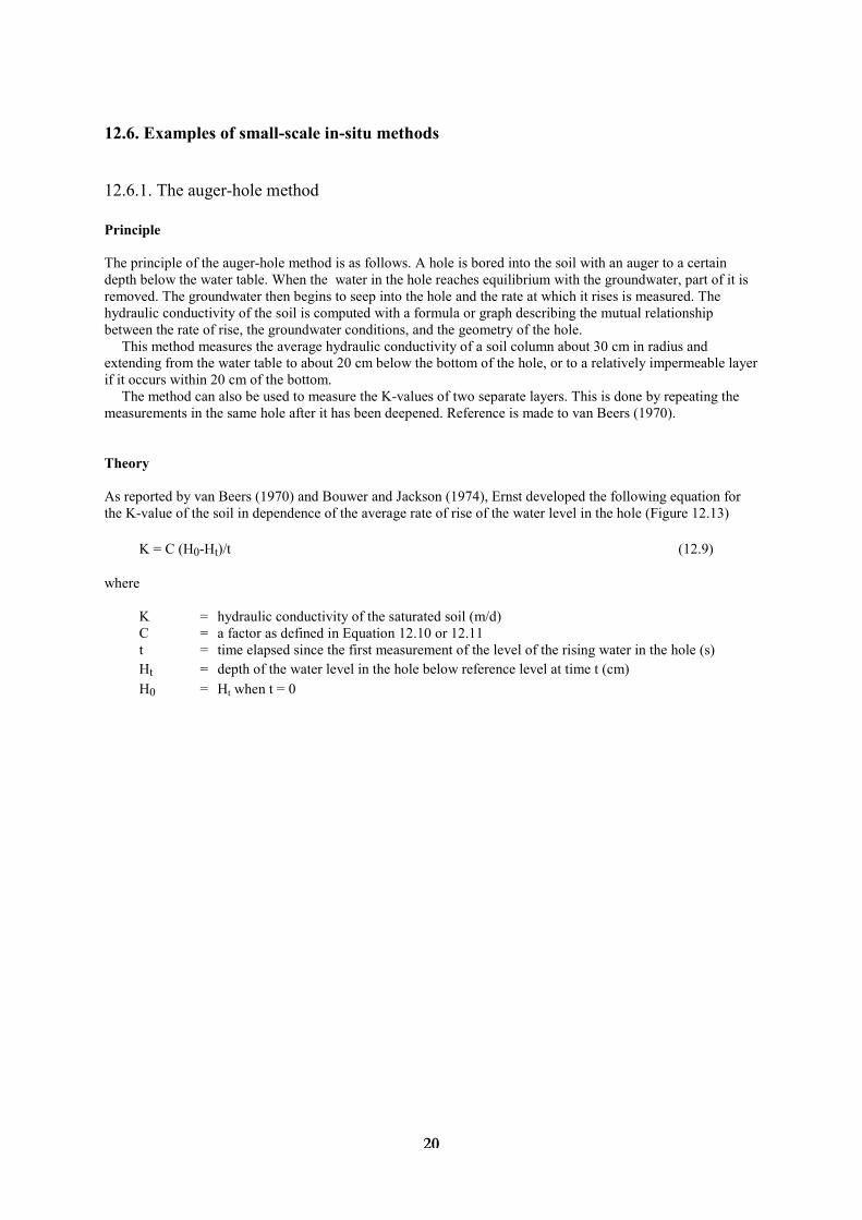
The principle of the auger-hole method is as follows. A hole is bored into the soil with an auger to a certain depth below the water table. When the water in the hole reaches equilibrium with the groundwater, part of it is removed. The groundwater then begins to seep into the hole and the rate at which it rises is measured. The hydraulic conductivity of the soil is computed with a formula or graph describing the mutual relationship between the rate of rise, the groundwater conditions, and the geometry of the hole. This method measures the average hydraulic conductivity of a soil column about 30 cm in radius and extending from the water table to about 20 cm below the bottom of the hole, or to a relatively impermeable layer if it occurs within 20 cm of the bottom. The method can also be used to measure the K-values of two separate layers. This is done by repeating the measurements in the same hole after it has been deepened. Reference is made to van Beers (1970). Theory

As reported by van Beers (1970) and Bouwer and Jackson (1974), Ernst developed the following equation for the K-value of the soil in dependence of the average rate of rise of the water level in the hole (Figure 12.13) K = C (H0-Ht)/t (12.9) where K = hydraulic conductivity of the saturated soil (m/d) C = a factor as defined in Equation 12.10 or 12.11 t = time elapsed since the first measurement of the level of the rising water in the hole (s) Ht = depth of the water level in the hole below reference level at time t (cm) H0 = Ht when t = 0

21

reference levelstandard

soil surface

tapewithf loat

D1

impermeable layer

water table

Ho

Ht

Dh

D2

D

ht

2 r

Figure 12.13 Measurements for the auger-hole method The C-factor depends on the depth of an impermeable layer below the bottom of the hole (D) and the average depth of the water level in the hole below the water table (h') as follows: When D > ½ D2, then 4000 r/ h' C = ------------------------ (12.10) (20+D2/r)(2-h’/D2) When D = 0, then 3600 r/ h' C = ------------------------ (12.11) (10+D2/r)(2-h’/D2) where D = depth of the impermeable layer below the bottom of the hole (cm) D2 = depth of the bottom of the hole below the water table (cm), with the condition: 20 < D2 <

200 r = radius of the hole (cm): 3 < r < 7 h' = average depth of the water level in the hole below the water table (cm), with the condition: h'

> D2/5

22

When 0 < D < ½ D2, one must interpolate between the results of the above two equations. The value of h' can be calculated from h' = 0.5 (H0 + Hn) - D1 (12.12) where D1 = depth of the water table below reference level (cm) Hn = depth of the water level in the hole at the end of the measurements (cm) Ernst also prepared graphs for the solution of the C-factor in Equation 12.9 (van Beers 1970), which are more accurate than Equations 12.10 and 12.11. Within the ranges of r and H mentioned above, however, the equations give less than 20% error. In view of the usually large variability in K-values (of the order of 100 to 1000%, or more), the given equations are accurate enough. Other methods of determining K-values with the auger-hole method were reviewed by Bouwer and Jackson (1974). These methods give practically the same results as the Ernst method. Equipment and Procedure

The equipment used in The Netherlands is illustrated in Figure 12.14. It consists of a tube, 60 cm long, the bottom end of which is fitted with a clack valve so that it can be used as a bailer. Extension pieces can be screwed to the top end of the tube. A float, a light-weight steel tape, and a standard are also part of the equipment. The standard is pressed into the soil down to a certain mark, so that the water-level readings can be taken at a fixed height above the ground surface. The hole must be made with a minimum disturbance to the soil. The open blade auger used in The Netherlands is very suitable for wet clay soils, whereas the closed pothole auger commonly used in the U.S.A. is excellent in dry soils.

Figure 12.14 Equipment used for the auger-hole method (van Beers 1970) The optimum depth of the holes depends on the nature, thickness, and sequence of soil layers, on the depth of the water table, and on the depth at which one wishes to determine the hydraulic conductivity. When augering the hole in slowly permeable soils, one often observes that the water is entering the hole only when the depth of the hole is well below the water table. As the hole is deepened further, the water enters faster, because the rate of inflow of the water is governed by the difference between the water table and the water level in the hole, and by the depth of the hole below reference level (D2). Sometimes, this phenomenon is incorrectly attributed to

23

artesian pressure, but artesian pressure only exerts an influence if one pierces a completely or almost impermeable layer. When the water in the hole is in equilibrium with the groundwater, the level is recorded. Water is then bailed out to lower the level in the hole by 20 to 40 cm. Measuring the rate of rise in the water level must begin immediately after bailing. Either the time for fixed intervals of rise, or the rise for fixed intervals of time can be recorded. The first technique requires the use of chronometers, while the second, which is customary in The Netherlands, needs only a watch with a good second hand. Normally, some five readings are taken, as these will give a reliable average value for the rate of rise and also provide a check against irregularities. The time interval at which water-level readings are taken is usually from 5 to 30 seconds, depending on the hydraulic conductivity of the soil, and should correspond to a rise of about 1 cm in the water level. A good rule of thumb is that the rate of rise in mm/s in an 8 cm diameter hole with a depth of 70 cm below the water table approximately equals the K-value of the soil in m/d. Care should be taken to complete the measurements before 25% of the volume of water removed from the hole has been replaced by inflowing groundwater. After that, a considerable funnel-shaped water table develops around the top of the hole. This increases resistance to the flow around and into the hole. This effect is not accounted for in the formulas or flow charts developed for the auger-hole method and consequently it should be checked that H0 - Ht < 0.25 (H0 - D1). After the readings have been taken, the reliability of the measurements should be checked. The difference in water level between two readings (∆H) is therefore computed to see whether the consecutive readings are reasonably consistent and whether the value of ∆H gradually decreases. It often happens that ∆H is relatively large for the first reading, because of water dripping along the walls of the hole directly after bailing. Further inconsistencies in ∆H values may be caused by the float sticking to the wall or by the wind blowing the tape against the wall. Consistency can be improved by tapping the tape regularly. An example of recorded data and the ensuing calculations is presented in Table 12.4. The auger-hole method measures the K-value mainly around the hole. It gives no information about vertical K-values nor about K-values in deeper soil layers. The method is therefore more useful in shallow than in deep aquifers.

24

Table 12.4 Example of measurements and calculations with the auger-hole method

Nr.: Date: Location: Details:

Depth of auger-hole D’ : 240 cm below reference Depth of water table D1 : 114 cm below reference D2 = D’ – D1 : 126 cm Auger-hole radius : 4 cm Depth impermeable layer : D > ¼ D2

t H ∆H *) (s) (cm) (cm)

---------------------------------------------------------------------------------------------------- 0 145.2 - 10 144.0 1.2 20 142.8 1.2 30 141.7 1.1 40 140.6 1.1 50 139.6 1.0

Try t = 50 s; ∆H50 = H0 – H50 = 145.2 –139.6 = 5.6 cm

Check H0 – H50 < 0.25 (H0 – D1); 145.2 – 139.6 < 0.25 (145.2 – 114); 5.6 < 7.8 → O.K. **)

Equation 12.12: h’ = 0.5 (145.2 + 139.6) – 114 = 28.4 cm

Ratio’s for Equation 12.10: D2/r = 31.5; h’/D2 = 28.4 r/h’ = 0.141

4000 x 0.141 Equation 12.10: C = ----------------------- = 6.2 (20+31.5)(2-0.225)

Equation 12.9: K = 6.2 x 5.6/50 = 0.7 m/day

*) per reading; ∆H = Ht-=1 – Ht **) if not O.K. try t = 40 s or less, so that ∆Ht decreases

12.6.2. Inversed auger-hole method

Principles and theory of the infiltration process

If one uses a steel cylinder (also called "infiltrometer") to infiltrate water continuously into unsaturated soil, one will find after a certain time that the soil around and below the area becomes almost saturated and that the wetting front is a rather sharp boundary between wet and dry soil (Figure 12.15). We shall consider a point just above the wetting front at a distance z below the soil surface in the area where the water infiltrates. The matric head of the soil at this point has a (small) value hm. The head at the soil surface

25

equals z + h (h = height of water level in the cylinder). The head difference between the point at depth z and a point at the soil surface equals z + h + |hm|, and the average hydraulic gradient between the two points is: S = (z + h + |hm|)/z (12.13) If z is large enough, s approximates unity. Hence, from Darcy's Law (Equation 12.2), we know that the mean flow velocity in the wetted soil below approaches the hydraulic conductivity (v = K), assuming the wetted soil is practically saturated.

water level

soil surface

cylinder wall

z

hinfil t rat ion surface

wet t ing front

Figure 12.15 Infiltration process beneath a cylinder infiltrometer The inversed auger-hole method (in French literature known as the "Porchet method") is based on these principles. If one bores a hole into the soil and fills this hole with water until the soil below and around the hole is practically saturated, the infiltration rate v will become more or less constant. The total infiltration Q will then be equal to v × A (where A is the surface area of infiltration). With v = K, we get: Q = K × A. For the inversed auger-hole method, infiltration occurs both through the bottom and the sidewalls of the hole (Figure 12.16). Hence we have A = πr2 + 2πrh (where r is the radius of the hole and h is the height of the water column in the hole). So we can write Q = 2πKr(h + ½ r). Further, we can find Q from the rate at which the water level in the hole is lowered: Q = -πr2dh/dt. Eliminating Q in both expressions gives 2K(h + ½ r) = r dh/dt. Upon integration and rearrangement, we obtain log (h0+½r) – log (ht+½r) K = 1.15 r ------------------------------ (12.14) t – t0 where (Figure 12.17) t = time since the start of measuring (s) ht = the height of the water column in the hole at time t (cm) h0 = ht at time t = 0

26

2 r

waterlevel

soil surface

auger hole

h

z

wetting

front

Figure 12.16 Infiltration from a water-filled auger-hole into the soil (inversed auger-hole method)

standard reference level

soil surface

tapewithf loat

2 r

ht

ho

Ho

Ht

D

Figure 12.17 Measurements for the inversed auger-hole method

27

The values of ht are obtained from ht = D' – Ht (12.15) where D' = the depth of the hole below reference level (cm) Ht = the depth of the water level in the hole below reference level (cm) When H and t are measured at appropriate intervals (as was explained in the previous section), K can be calculated. On semilog paper, plotting ht + ½r on the log axis and t on the linear axis produces a straight line with a slope: log (h0+½r) – log (ht+½r) tan α = ------------------------------ (12.16) t – t0 The calculation of K with Equation 12.14 can therefore also be done with the value of tan α. Hence: K = 1.15 r tan α.

Procedure

After a hole is made in the soil to the required depth, the hole is filled with water, which is left to drain away freely. The hole is refilled with water several times until the soil around the hole is saturated over a considerable distance and the infiltration (rate) has attained a more or less constant value. After the last refilling of the hole, the rate of drop of the water level in the hole is measured (e.g. with the float and tape system as was explained for the auger-hole method). The data (h + ½r and t) are then plotted on semi-log paper, as was explained earlier. The graph should yield a straight line. If the line is curved, continue to wet the soil until the graph shows the straight line. Now, with any two pairs of values of h + ½r and t, the K value can be calculated according to Equation 12.14. An example of measurements is given in Table 12.5. Table 12.5 Example of measurements with inversed auger-hole method (r = 4 cm, D' = 90 cm) t Ht ht = D’ – Ht h1 + ½r 0 71 19 21 140 72 18 20 300 73 17 19 500 74 16 18 650 75 15 17 900 76 14 16 The data of Table 12.5 are plotted in Figure 12.18, which shows that a linear relation exists between log(ht + ½r) and t. The K-value can now be calculated from Equation 12.14 as follows: t0= 140 h0 + ½r = 20 log(h0 + ½r) = 1.30 t = 650 ht + ½r = 17 log(ht + ½r) = 1.23 1.30 – 1.23 K = 1.15 x 4 ------------- 650 – 140

28

0 500 1000

10

12

14

16

18

20

25

30

t in s

h + in cmtr2

�

Figure 12.18 Fall of the water level, recorded with the inversed auger-hole method, plotted against time (the symbol indicating the slope of the line should be α)

12.7. Examples of methods using parallel drains

12.7.1. Introduction When one is analysing the relationships between hydraulic head (elevation of the water table) and the discharge of pipe drainage systems to assess the soil's hydraulic conductivity, one needs a drainage equation in agreement with the conditions during which the measurements were made. Usually, the measurements are made during a dry period following a period of recharge by rain or irrigation (i.e. during tail recession). Hence, the water table is falling after it had risen as a result of the recharge. Under such non-steady state conditions, Equation 8.36 (Chapter 8) is applicable for ideal drains (i.e. drains without entrance resistance) qL2 = 2π Kb d h (12.17) which can be extended to include the flow above the drain level (Oosterbaan et al. 1989) qL2 = 2π Kb d h + π Ka h2 (12.19) where: q = drain discharge (m/d) Kb = hydraulic conductivity of the soil below drain level (m/d) Ka = hydraulic conductivity of the soil above drain level (m/d) d = Hooghoudt's equivalent depth (m) h = elevation of the water table midway between the drains relative to drain level (m) L = drain spacing (m) Since entrance resistance is not always negligible, Oosterbaan et al. (1989) showed that Equation 12.17 can be adjusted to take the entrance head into account (Figure 12.19):

29

qL2 = 2π Kb (h-hc) + π Ka (h-hc)(h+hc) (12.18) or qL2 = 2π Kb h' + π Ka h' h* (12.19) where, in addition to the previously defined symbols: he = entrance head (i.e. the elevation of the water table above the drains relative to drain level)

(m) h' = h - he; available hydraulic head (i.e. the elevation of the water table midway between the

drains relative to drainage level) (m) h* = h + he (m)

soil surface

impermeable layer

L12

drainage level

water divide

drain level

h h

he

Dd

drain

water

table

Figure 12.19 Drains with entrance resistance (symbols as defined for Equations 12.17 - 12.19) The equivalent depth d, which is a function of the depth to the impermeable layer D, the drain spacing L, and the drain radius ro, can be determined according to the flow chart in Figure 8.4 (Chapter 8), and the wet perimeter, u, can be chosen according to Section 8.2.2. In theory, the d-value must be calculated with an adjusted radius r' = ro + he instead of ro, and the factor 8 must be replaced by 2π, but neglecting this does not usually lead to any appreciable error in the K-values. The procedures discussed in the following sections are based on Equations 12.18 and 12.19. Statistical methods (Chapter 6, Section 6.5.4) are used to account for random variations.

12.7.2. Procedures of analysis To determine the K-value in an area with existing drains, one observes the depth of the water table midway between the drains, and near the drains, and converts the measurements to hydraulic-head and entrance-head values, respectively. Observations should be made in one or more cross-sections over the drains, at different times during periods of tail recession. The drain discharge is measured at the same time. The measured discharge in m3/d should be expressed per unit surface area of the zone of influence of the drain (i.e. the drain length multiplied by the drain spacing), obtaining q in m/d. Equation 12.19 may also be written as:

30

q/ h' = a h* + b (12.20) with a = π Ka/L

2 and b = 2π Kb d /L2 Plotting the values of q/h' on the vertical axis against the values of h* on the horizontal axis may result in one of the different lines depicted in Figure 12.20. According to the type of line, one follows different procedures, as will be explained below.

q / h

h* in m

plot of q / h versus h*, (h = h - h h* = h + h )

in d -1

I

IVIIIII

e e Figure 12.20 Different patterns in plotted field data on drain discharge and hydraulic head;

1) No resistance to flow above drain level; 2) No resistance to flow below drain level; 3) Resistance to flow occurs above and below drain level; 4) Similar to pattern 2, but with a high entrance head

Procedure 1

Procedure 1 is used if q/h' plotted against h* yields a horizontal line (Type I in Figure 12.20). The value of a (Equation 12.20) is close to zero, so the flow above drain level can be neglected. Consequently, the hydraulic resistance is mainly due to flow below drain level. For each set of (q, h, he) data, and the equivalent depth, d, from Chapter 8, we calculate the hydraulic conductivity, Kb, using Equation 12.20 with a = 0: Kb = q L2 / (2π d h') = b L2 / (2π d) (12.21) We then determine the mean value of Kb, its standard deviation, and the standard deviation of the mean. We find the upper and lower confidence limits of Kb, using Student's t-distribution, as was explained in Chapter 6, Section 6.5.2. Procedure 1 will be used in Example 12.3 (Section 12.7.3). Procedure 2

Procedure 2 is used if q/h' plotted against h* yields a straight line of Type II (Figure 12.20). The slope of the line, a, (Equation 12.20) represents the value of the hydraulic conductivity above drain level. The line passes through the origin; the zero intercept points towards a negligible flow below drain level. These drains are resting on an impermeable layer. With each set of (q, h, he) data, we calculate the Ka- value, using Equation 12.20 with b = 0: Kb = q L2 / (2π h* h') = a L2 / π (12.22)

31

We then determine the mean and standard deviation of Ka, and the standard deviation of the mean. With Student's t-distribution, we find confidence limits of Ka and of Ka (Section 6.5.2). Procedure 2 will be used in Example 12.4 (Section 12.7.4). Procedure 3

Procedure 3 is used if q/h' plotted against h* yields a straight line that does not pass through the origin (Type III in Figure 12.20). In this case, there is flow above and below the drain level, and neither Ka nor Kb can be neglected. We then perform a linear two-way regression analysis with the equations q/h' = a h* + b (12.23) and h*= a' (q/h')+ b' (12.24) Writing Equation 12.24 in the same form as Equation 12.23 gives q/h' = (h*/a') - b' We thus find two different regression coefficients, a and 1/a', which we can combine into an intermediate regression coefficient, a*, by taking their geometric mean. Also, we find an intermediate value b* (Chapter 6, Section 6.5.4). Using Equation 2.20, we can find the Ka nor Kb values from the intermediate values a* and b* instead of a and b. Following Chapter 6, the confidence limits of Ka nor Kb are found from the confidence limits of a* and b*. The width of the confidence intervals will be somewhat underestimated, because the variables q/h' and h* are not fully independent since both h' and h* contain parameters h and he. Often, a simpler procedure for finding the confidence limits can be used, because the two values a (from Equation 12.23) and 1/a' (from Equation 12.25) give a reasonable approximation of the confidence limits of a*. Similarly, we find the approximate confidence limits of b* as b and b'/a'. Example 12.5 will use Procedure 3, including these approximations of the confidence intervals. Procedure 4

Procedure 4 is used if q/h' plotted against h* yields an upward-bending curve which passes through the origin (Type IV in Figure 12.20). In this case, there is no flow below drain level and Kb can be neglected. The Ka value is not constant, but decreases with depth. We write Ka = λ h*, so that substitution into Equation 12.19 with Kb = 0 yields q/ h' = π λ h*2 / L2 Now, a plot of q/h' versus h*2 may yield a straight line going through the origin (Figure 12.21). Next, for each set of (q, h, he) data, we calculate the λ-value. We then determine its mean, and standard deviations of λ and . With Student's t-distribution, we can find the confidence limits of λ and. An example of this procedure was given by Oosterbaan et al. (1989).

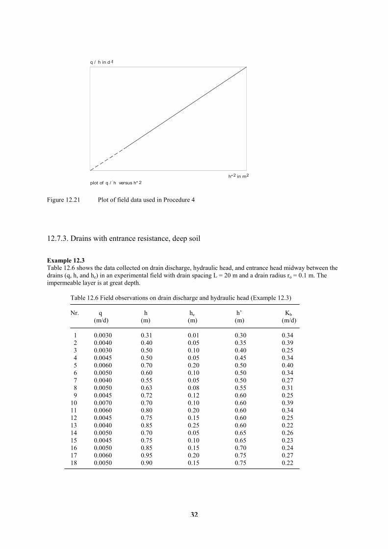
32

q / h in d -1

h* in m2 2

plot of q / h versus h* 2

Figure 12.21 Plot of field data used in Procedure 4

12.7.3. Drains with entrance resistance, deep soil

Example 12.3

Table 12.6 shows the data collected on drain discharge, hydraulic head, and entrance head midway between the drains (q, h, and he) in an experimental field with drain spacing L = 20 m and a drain radius ro = 0.1 m. The impermeable layer is at great depth.

Table 12.6 Field observations on drain discharge and hydraulic head (Example 12.3)

Nr. q h he h’ Kb (m/d) (m) (m) (m) (m/d)

1 0.0030 0.31 0.01 0.30 0.34 2 0.0040 0.40 0.05 0.35 0.39 3 0.0030 0.50 0.10 0.40 0.25 4 0.0045 0.50 0.05 0.45 0.34 5 0.0060 0.70 0.20 0.50 0.40 6 0.0050 0.60 0.10 0.50 0.34 7 0.0040 0.55 0.05 0.50 0.27 8 0.0050 0.63 0.08 0.55 0.31 9 0.0045 0.72 0.12 0.60 0.25 10 0.0070 0.70 0.10 0.60 0.39 11 0.0060 0.80 0.20 0.60 0.34 12 0.0045 0.75 0.15 0.60 0.25 13 0.0040 0.85 0.25 0.60 0.22 14 0.0050 0.70 0.05 0.65 0.26 15 0.0045 0.75 0.10 0.65 0.23 16 0.0050 0.85 0.15 0.70 0.24 17 0.0060 0.95 0.20 0.75 0.27 18 0.0050 0.90 0.15 0.75 0.22

33

A plot of q/h' versus h* values (Figure 12.22) shows that the envelope lines tend to be horizontal, indicating that resistance to flow above drain level can be neglected. Hence, Procedure 1 and Equation 12.21 are applicable. According to Table 8.1 (Chapter 8), Hooghoudt's equivalent depth d = 1.89 m. The Kb-values thus found are shown in Table 12.6.

0

0 0.2 0.4 0.6 0.8 1.0 1.2

0.0025

0.0075

0.0050

0.0100

0.0125

0.0150

q / h in d-1

hydraulic head h* in m

upper envelope

lower envelope

Figure 12.22 Plot of field data indicating a negligible flow resistance above drain level (Example 12.3) The Kb-values in Table 12.6 have a mean value Kb = 0.30 m/d. The standard deviation of the mean is 0.014 m/d. Using Student's probability distribution (Section 6.5.2) for a 90% confidence interval and 17 degrees of freedom (tf = 1.75), we can state with 90% confidence that 0.28 < Kb < 0.32 m/d

12.7.4. Drains with entrance resistance, shallow soil Example 12.4

Table 12.7 shows the data collected in experimental fields in the delta of the Tagus River in Portugal, in which corrugated and perforated PVC pipe drains with a radius ro = 0.10 m were installed at a depth of 1.1 m below the soil surface and at a spacing L = 20 m. The soils in this delta are fine textured (heavy clay soil).

34

Table 12.7 Field observations on drain discharge and hydraulic head (Example 12.4)

No. Date q h he h’ h* q/h’ Ka (m/d) (m) (m) (m) (m) (d-1) (m/d)

1 29/12 0.00137 0.88 0.18 0.70 1.06 0.00196 0.235 2 30/12 0.00106 0.85 0.13 0.72 0.98 0.00147 0.191 3 31/12 0.00064 0.73 0.08 0.65 0.81 0.00098 0.155 4 02/01 0.00300 0.61 0.03 0.58 0.64 0.00052 0.103 5 03/01 0.00026 0.58 0.02 0.56 0.60 0.00046 0.099 6 07/01 0.00129 0.82 0.16 0.66 0.98 0.00195 0.254 7 08/01 0.00124 0.84 0.18 0.66 1.02 0.00188 0.235 8 09/01 0.00126 0.82 0.12 0.70 0.94 0.00180 0.244 9 10/01 0.00084 0.77 0.10 0.67 0.87 0.00125 0.183 10 13/01 0.00035 0.50 0.01 0.49 0.51 0.00071 0.178 11 21/01 0.00303 0.98 0.54 0.44 1.52 0.00698 0.577 12 22/01 0.00263 0.96 0.45 0.51 1.41 0.00516 0.406 13 25/01 0.00129 0.91 0.20 0.71 1.11 0.00182 0.208 14 26/02 0.00086 0.88 0.18 0.70 1.06 0.00123 0.148 15 28/02 0.00043 0.73 0.01 0.72 0.74 0.00060 0.103 16 03/03 0.00027 0.53 0.00 0.53 0.53 0.00051 0.122 17 05/03 0.00040 0.69 0.02 0.67 0.71 0.00060 0.107 18 06/03 0.00031 0.61 0.01 0.60 0.62 0.00052 0.106 19 07/03 0.00026 0.60 0.00 0.60 0.60 0.00043 0.092

Figure 12.23A shows the drainage intensity, q/h', plotted against the h*-values of Table 12.7. The relation between q/h' and h* shows an upward-bending curve through the origin of the graph. This suggests that the soil below drain level is impermeable and that the soil above drain level has a K-value that decreases with depth. If we ignore the two highest points in Figure 12.23A, however, we can make the assumption that the relationship between q/h' and h* gives a straight line through the origin of the graph or, in other words, that the soil above drain level has a constant K-value, whereas the resistance to flow below the drains is neglected. This assumption is illustrated by the straight line in Figure 12.23A. Hence, Procedure 2 is used and the hydraulic conductivity Ka is calculated according to Equation 12.22. Table 12.7 shows the results. The mean Ka equals 0.20 m/d. The standard deviation of Ka = 0.13 m/d and the standard deviation of Ka = 0.032 m/d. We can calculate the confidence interval of the mean Ka using Student's t-distribution (Section 6.5.2). With 90% confidence and n-1=18 degrees of freedom we find it to range from 0.14 to 0.26 m/d. Discussion

As stated earlier, the procedure for the calculation can be improved by accepting that the value of Ka decreases with depth, as occurs frequently in heavy clay soils. This is also suggested in Table 12.7, by the decrease in the Ka-values with decreasing q- and h-values. Oosterbaan et al. (1989) calculated that the Ka-value is 0.77 m/d at the soil surface, 0.22 m/d at 0.55 m depth, and almost zero at drain level. From this analysis, it follows that the drains are situated in a slowly permeable soil layer, which explains the presence of the entrance resistance. It is likely that the entrance head would have been less if the drains had been placed less deeply. In soils like those found in the experimental plot, the optimum drain depth is probably about 0.8 m. Figure 12.23B, which shows a plot of q against he, indicates that the entrance head increases proportionally with the discharge. This corresponds to the previous conclusion that the Ka-value is small at drain depth.

35

0

00 0.15 0.30 0.45 0.60

entrance head h in me

0 0.2 0.4 1.00.6 1.20.8 1.4 1.6

0.002

0.0010

0.001

0.0005

0.003

0.0015

0.004

0.0020

0.005

0.0025

0.006

0.0030

0.007

-1

A

B

0.0035

drain discharge q in m / d

q / h in d

hydraulic head h* in m

Figure 12.23 Plots of field data from the Leziria Grande (Example 12.4) A: The hydraulic conductivity above the drains decreases with depth B: Plot of drain discharge against entrance head

12.7.5. Ideal drains, medium soil depth

Example 12.5

Table 12.8 shows data on h and q in an experimental field with drain spacing L = 20 m and drain radius ro = 0.1 m. The entrance resistance was assumed to be negligibly small, so the he-values were not measured. Hence, the drains are supposed to function as ideal drains and he = 0. Note that h' = h* = h.

36

Table 12.8 Data on drain discharge and available hydraulic head used in Example 12.5

No. q h q/h (m/d) (m) (m/d)

1 0.00125 0.16 0.00781 2 0.00099 0.17 0.00282 3 0.00137 0.18 0.00761 4 0.00132 0.20 0.00660 5 0.00274 0.28 0.00979 6 0.00342 0.32 0.01069 7 0.00316 0.34 0.00929 8 0.00483 0.35 0.01380 9 0.00414 0.38 0.01089 10 0.00342 0.38 0.00900 11 0.00570 0.41 0.01390 12 0.00482 0.43 0.01121

A plot of q/h versus h-values (Figure 12.24) suggests that the relationship between these two parameters is an upward-sloping straight line that does not pass through the origin, indicating that the flow to the drains occurs above and below the drain level. Procedure 3 can therefore be applied, and a regression analysis is made. Applying the principles explained in Section 12.7.2 and using Equations 12.23 to 12.25, we find a) Regression of q/h upon h q/h = 0.021 h + 0.0035 b) Regression of h upon q/h h = 30.9 (q/h) + 0.00058 or q/h = 0.032h – 0.000019 The calculation of the K-values proceeds as follows. Using Equation 12.20, a = 0.021 yields Ka = 2.6 m/d, and 1/a' = 0.032 yields Ka = 4.1 m/d. Using these values as the approximate confidence limits, we find that 2.6 < Ka < 4.1 m/d. Similarly, b = 0.0035 yields Kb = 0.22 m2/d, and b'/a' = -0.000019 yields Kbd = -0.0012 m2/d. A comparison of the Ka - and Kbd-values shows that the Ka -value is the dominating one, and that the Kbd-value is statistically insignificant. Note that if we assume that the flow below drain level can be neglected, we can use Procedure 2 to analyse the data of Example 12.5 as well. This would give Ka = 4.3 m/d, with a standard deviation of the mean of 0.26 m/d.

37

0.002

0.004

0.006

0.008

0.010

0.012

0.014

0.016

q / h in d-1

00

0.20.1 0.3 0.4 0.5

hydraulic head h in m Figure 12.24 Plot of field data indicating flow above and below the drain level (Example 12.5) References Abrol, I.P., J.S.P. Yadav, and F.I. Massoud 1988. Salt-affected soils and their management. FAO Soils Bulletin

39, Rome, 131 p. Amer, M.H. and N.A. de Ridder 1989. Land drainage in Egypt. DRI, Cairo. 377 p. Anderson, S.H., and D.K. Cassel 1986. Statistical and autoregressive analysis of soil physical properties of

Portsmouth sandy loam. Soil Science Society of American Journal 50, pp. 1096-1104. Aronovici, V.S. 1947. The mechanical analysis as an index of subsoil permeability. Soil Science Society of

American Proc. 11, pp. 137-141. Ayers, R.S., and D.W. Westcott 1985. Water quality for agriculture. Rev. ed. Irrigation and Drainage Paper 29,

FAO, Rome, 174 p. Bentley, W.J., R.W.Skaggs, and J.E. Parsons 1989. The effect of variation in hydraulic conductivity on water

table drawdown. Technical Bulletin, North Carolina Agricultural Research Service, North Carolina State University, 288, Raleigh, 23 p.

Bouma, J., A. Jongerius, and D. Schoonderbeek 1979. Calculation of saturated hydraulic conductivity of some pedal clay soils using micromorphometric Data. Soil Science Society of American Journal 43, pp. 261-264.

Bouma, J., J.W. van Hoorn, and G.H. Stoffelsen 1981. Measuring the hydraulic conductivity of soil adjacent to tile drains in a heavy clay soil in The Netherlands. Journal of Hydrology 50, pp. 371-381.

Boumans, J.H. 1976. Drainage calculations in stratified soils using the anisotropic soil model to simulate hydraulic conductivity conditions. In: J. Wesseling (ed.), Proceedings of the international drainage workshop. ILRI Publication 25, Wageningen, pp. 108-123.

Bouwer, H., and R.D. Jackson 1974. Determining soil properties. In: J. van Schilfgaarde (ed.), Drainage for Agriculture. Agronomy 17. American Society of Agronomy, Madison, pp. 611-672.

Camp, C.R. 1977. Determination of hydraulic conductivity for a Louisiana alluvial soil. Third National Drainage Symposium Proceedings. American Society Agricultural Engineers, Michigan, pp. 1-77.

Childs, E.C. 1943. The water table, equipotentials and streamlines in drained land. Soil Science 56, pp. 317-330. De Ridder, N.A. and K.E. Wit 1965. A comparative study on the hydraulic conductivity of unconsolidated

sediments. Journal of Hydrology 3, pp. 180-206. Dieleman, P.J., and B.D. Trafford 1976. Drainage testing. Irrigation and Drainage Paper 28, FAO, Rome, 172 p. El-Mowelhi, N.M., and J. van Schilfgaarde 1982. Computation of soil hydrological constants from field

drainage experiments in some soils in Egypt. Transaction of the American Society Agricultural Engineers, pp. 77-79.

38

Kuntze, H. 1964. Einflusz der Dränung auf die Struktur des Marsch Bodens. Zeitschrift für Kulturtechnik und Flurbereinigung 5 (3), pp. 129-134.

Marshall, T.J. 1957. Permeability and the size distribution of pores. Nature 180, pp. 664-665. Oosterbaan, R.J., A. Pissarra, and J.G. van Alphen 1989. Hydraulic head and discharge relations of pipe

drainage systems with entrance resistance. Proceedings 15th European Regional Conference on Agricultural Water Management. Vol. III. ICID, Dubrovnik, pp. 86-98.

Oosterbaan, R.J. 1990a. Single pipe drains with entrance resistance above a semi-confined aquifer. In: Symposium on Land Drainage for Salinity Control, Vol. 3. Cairo, pp. 36-46.

Oosterbaan, R.J. 1990b. Parallel pipe drains with entrance resistance above a semi-confined aquifer with upward seepage. In: Symposium on Land Drainage for Salinity Control, Vol. 3. Cairo, pp. 26-35.

Oosterbaan, R.J. and H.P. Ritzema 1992. Hooghoudt's drainage equation, adjusted for entrance resistance and sloping land. In: W.F. Vlotman (ed.), Proceedings 5th International Drainage Workshop, Vol. II. ICID/WAPDA, Lahore, pp. 2.18-2.28.

Reynolds, W.D., and D.E. Elrick 1985. In-situ measurement of field saturated hydraulic conductivity, sorptivity, and the a-parameter, using the Guelph permeameter. Soil Science, 140, 4, pp. 292-302.

Richards, L.A. (ed.) 1954. Diagnosis and improvement of saline and alkaline soils. Agriculture Handbook 60. USDA, Washington, 160 p.

Scheltema, W. and H.Ch.P.M. Boons 1973. Al-clay, a solution to mechanical stability problems in a heavy clay soil? In: H. Dost (ed.), Acid sulphate soils : proceedings of the international symposium on acid sulphate soils. Vol. II. ILRI Publication 18, Wageningen, pp. 319-342.

Smedema, L.K., and D.W. Rycroft 1983. Land drainage : planning and design of Agricultural Drainage Systems. Batsford, London, 376 p.

Van Beers, W.F.J. 1970. The auger-hole method : a field measurement of the hydraulic conductivity of soil below the water table. Rev. ed. ILRI Bulletin 1, Wageningen, 32 p.

Van Hoorn, J.W. 1958. Results of a groundwater level experimental field with arable crops on a clay soil. Netherlands Journal Agricicultural Science, 6, pp. 1-10.

Wit, K.E. 1967. Apparatus for measuring hydraulic conductivity of undisturbed soil samples. Technical Bulletin 52. Institute for Land and Water Management Research, Wageningen, 12 p.

Wösten, J.H.M. 1990. Use of soil survey data to improve simulation of water movement in soils. Thesis, Agricultural University, Wageningen, 103 p.

Zangar, C.N. 1953. Theory and problems of water percolation. U.S. Bureau of Reclamation. Engineering Monograph No. 8, Denver, 76 p.