Probability Distributions of Hydraulic Conductivity for ... · Probability Distributions of...

Prepared in cooperation with theU.S. DEPARTMENT OF ENERGYNATIONAL NUCLEAR SECURITY ADMINISTRATIONNEVADA OPERATIONS OFFICE, underInteragency Agreement DE-AI08-01NV13944

Probability Distributions of Hydraulic Conductivity for the Hydrogeologic Units of the Death Valley Regional Ground-Water Flow System, Nevada and California

U.S. Department of the InteriorU.S. Geological Survey

Water-Resources Investigations Report 02–4212

(Back of Cover)

Probability Distributions of Hydraulic Conductivity for the Hydrogeologic Units of the Death Valley Regional Ground-Water Flow System, Nevada and California

By Wayne R. Belcher, Donald S. Sweetkind, and Peggy E. Elliott

U.S. GEOLOGICAL SURVEY

Carson City, Nevada2002

Prepared in cooperation with theU.S. DEPARTMENT OF ENERGYNATIONAL NUCLEAR SECURITY ADMINISTRATIONNEVADA OPERATIONS OFFICE, underInteragency Agreement, DE-AI08-01NV13944

Water-Resources Investigations Report 02-4212

U.S. DEPARTMENT OF THE INTERIORGALE A. NORTON, Secretary

U.S. GEOLOGICAL SURVEYCHARLES G. GROAT, Director

Any use of trade, product, or firm names in this publication is for descriptivepurposes only and does not imply endorsement by the U.S. Government

For additional informationcontact:

District Chief U.S. Geological Survey333 West Nye Lane, Room 203Carson City, NV 89706–0866

email: [email protected]

URL: http://nevada.usgs.gov

CONTENTS

Abstract.................................................................................................................................................................................. 1Introduction............................................................................................................................................................................ 1

Location...................................................................................................................................................................... 2Purpose and Scope ..................................................................................................................................................... 2Limitations ................................................................................................................................................................. 2Acknowledgments...................................................................................................................................................... 2

Hydrogeologic Setting ........................................................................................................................................................... 4Regional Overview..................................................................................................................................................... 4Hydrogeologic Units .................................................................................................................................................. 4

Data Analysis and Synthesis.................................................................................................................................................. 4Estimating Probability Distributions.......................................................................................................................... 5Statistical Hypothesis Testing .................................................................................................................................... 5

Probability Distributions........................................................................................................................................................ 5Basin-Fill Hydrogeologic Units ................................................................................................................................. 5Bedrock Confining Hydrogeologic Units .................................................................................................................. 9Carbonate Rock Hydrogeologic Units ....................................................................................................................... 9Volcanic Rock Hydrogeologic Units.......................................................................................................................... 9Applicability of Distributions to a Regional Model................................................................................................... 14Principle of Parsimony ............................................................................................................................................... 14

Summary................................................................................................................................................................................ 17References Cited.................................................................................................................................................................... 17

FIGURES

1. Location map of study area .................................................................................................................................... 32–8. Graphs showing hydraulic-conductivity distributions for:

2. Basin-fill hydrogeologic units............................................................................................................................ 83. Regional bedrock confining hydrogeologic units .............................................................................................. 104. Carbonate rock hydrogeologic units .................................................................................................................. 115. Tertiary volcanic rock hydrogeologic units........................................................................................................ 126. Tertiary volcanic rock lithologies....................................................................................................................... 137. Welding in ash-flow tuffs ................................................................................................................................... 158. Alteration in ash-flow tuffs ................................................................................................................................ 16

TABLES

1. Horizontal hydraulic-conductivity estimates of hydrogeologic units in the Death Valley regional ground-water flow system................................................................................. 6

2. Horizontal hydraulic-conductivity estimates of volcanic rock hydrogeologic units in the Death Valley regional ground-water flow system ........................................................................ 7

3–9. Results of hypothesis testing for:3. Basin-fill hydrogeologic units............................................................................................................................ 84. Bedrock confining units ..................................................................................................................................... 105. Carbonate rocks.................................................................................................................................................. 116. Tertiary volcanic rock hydrogeologic units........................................................................................................ 127. Tertiary volcanic rock lithologies....................................................................................................................... 138. Welding in ash-flow tuffs ................................................................................................................................... 159. Alteration in tuffs ............................................................................................................................................... 16

CONTENTS III

CONVERSION FACTORS, VERTICAL DATUM, AND ACRONYMS

Multiply By To obtain

meter (m) 3.2808 footmeter per day (m/d) 3.2808 foot per day

square kilometer (km2) 0.3861 square mile

Temperature: Degrees Celsius (oC) can be converted to degrees Fahrenheit (oF) by using the formula oF = [1.8(oC)]+32. Degrees Fahrenheit can be converted to degrees Celsius by using the formula oC = 0.556(oF-32).

Sea level: In this report, “sea level” refers to the National Geodetic Vertical Datum of 1929 (NGVD of 1929, formerly called “Sea-Level Datum of 1929”), which is derived from a general adjustment of the first-order leveling networks of the United States and Canada.

ACRONYMS USED IN THIS REPORT

AA Alluvial aquifer NTS Nevada Test SiteACU Alluvial confining unit OVU Older volcanics unitBRU Belted Range unit PVA Paintbrush volcanic aquiferCFBCU Crater Flat-Bullfrog confining unit SCU Sedimentary confining unitCFPPA Crater Flat-Prow Pass aquifer TMVA Thirsty Canyon/Timber Mountain volcanic aquiferCFTA Crater Flat-Tram aquifer TV Tertiary volcanicsCHVU Calico Hills volcanic unit UCA Upper carbonate aquiferDVRFS Death Valley regional ground-water flow system UCCU Upper clastic confining unitHGU Hydrogeologic unit VSU Volcaniclastics and sediments unitICU Intrusive confining unit WVU Wahmonie volcanic unitLCA Lower carbonate aquifer YVU Younger volcanic unitLCCU Lower clastic confining unit XCU Crystalline confining unitLFU Lava flow unit

IV Probability Distribution of Hydraulic Conductivity for the Hydrogeologic Units of the DVRFS, Nevada and California

PROBABILITY DISTRIBUTIONS OF HYDRAULIC CONDUCTIVITY FOR THE HYDROGEOLOGIC UNITS OF THE DEATH VALLEY REGIONAL GROUND-WATER FLOW SYSTEM, NEVADA AND CALIFORNIA

By Wayne R. Belcher, Donald S. Sweetkind, and Peggy E. Elliott

ABSTRACT

The use of geologic information such as lithology and rock properties is important to con-strain conceptual and numerical hydrogeologic models. This geologic information is difficult to apply explicitly to numerical modeling and analy-ses because it tends to be qualitative rather than quantitative. This study uses a compilation of hydraulic-conductivity measurements to derive estimates of the probability distributions for sev-eral hydrogeologic units within the Death Valley regional ground-water flow system, a geologically and hydrologically complex region underlain by basin-fill sediments, volcanic, intrusive, sedimen-tary, and metamorphic rocks. Probability distribu-tions of hydraulic conductivity for general rock types have been studied previously; however, this study provides more detailed definition of hydro-geologic units based on lithostratigraphy, lithol-ogy, alteration, and fracturing and compares the probability distributions to the aquifer test data. Results suggest that these probability distributions can be used for studies involving, for example, numerical flow modeling, recharge, evapotranspi-ration, and rainfall runoff. These probability distri-butions can be used for such studies involving the hydrogeologic units in the region, as well as for similar rock types elsewhere.

Within the study area, fracturing appears to have the greatest influence on the hydraulic con-ductivity of carbonate bedrock hydrogeologic units. Similar to earlier studies, we find that alter-ation and welding in the Tertiary volcanic rocks greatly influence hydraulic conductivity. As

alteration increases, hydraulic conductivity tends to decrease. Increasing degrees of welding appears to increase hydraulic conductivity because weld-ing increases the brittleness of the volcanic rocks, thus increasing the amount of fracturing.

INTRODUCTION

The U.S. Geological Survey (USGS) is develop-ing a three-dimensional ground-water flow model of the Death Valley regional ground-water flow system (DVRFS). This area lies within the southern Great Basin section of the Basin and Range physiographic province and surrounds both the Nevada Test Site (NTS), where nuclear weapons tests have contaminated the ground water beneath some areas, and Yucca Mountain, which is being investigated for its suitability for permanent storage of high-level nuclear waste in a mined geologic repository. As a result of this area’s importance and intensive studies, an extensive geologic and hydrologic data set exists for a large, regional sys-tem.

Bedinger and others (1989) produced a series of probability distributions for rock types common to the Basin and Range physiographic province. Data used to prepare these distributions consisted of published field and laboratory tests within the Basin and Range prov-ince, as well as general studies from rocks with similar characteristics from outside the Basin and Range prov-ince (Bedinger and others, 1989, p. 18). This work dif-fers in that we use only compiled field data for the rock types found in the region. This study uses the hydro-geologic unit assignments based on Laczniak and oth-ers (1996) developed at the NTS, and thus is more detailed than the regional definitions provided by Bedinger and others (1989). Hydrogeologic units are rock units grouped according to their water-storage and

ABSTRACT 1

transmissive properties (Laczniak and others, 1996). Relations between secondary processes such as fractur-ing and alteration that affect measured hydraulic con-ductivity also are examined.

Location

The DVRFS is in southeastern California and Nevada (fig. 1). The DVRFS encompasses about 45,000 km2 within the Great Basin section of the Basin and Range physiographic province. The area for this study is considerably larger than the DVRFS in order to include areas that contain sites important to defining hydraulic-property estimates for units contained within the DVRFS. The topography typically consists of northerly and northwesterly trending mountain ranges surrounded by broad sediment-filled basins. The Spring Mountains, the highest topographic feature in the area, are about 3,600 m above mean sea level. Other prominent topographic features within the region include the Sheep Range, Pahute Mesa, the Funeral Mountains, and the Panamint Range. Basins generally decrease in altitude from north to south. The lowest altitude at 86 m below sea level in the study area is at Badwater in Death Valley National Park.

Purpose and Scope

The purpose of this report is to present statistical-probability distributions that can be used by hydrolo-gists to constrain hydraulic-conductivity estimates in their studies. These distributions could be useful for hydrologic studies involving numerical simulations of ground water, recharge, rainfall runoff, evapotranspira-tion, basin analyses, and water budgets. Other uses of the distributions could include contaminant-transport modeling, water-supply issues, and resource protec-tion. The probability distributions also could be used to apply the principle of parsimony (Hill, 1998, p. 35) to simulation efforts. Specifically, the work presented in this report is for use in a transient numerical ground-water flow model of the DVRFS, but because of the diversity of rock types within the study area, these dis-tributions may be useful to flow modelers in other regions and other types of studies for which hydraulic-conductivity information is required.

Limitations

The analyses in this report have several limita-tions:

1. The hydraulic-conductivity measurements pre-sented in this report are based mostly on the results of field-scale tests and represent a very small part of an overall regional HGU. Lithologic factors that can affect hydraulic conductivity, such as facies changes in sedimentary rock, welding and alteration in volca-nic rocks, and degree of fracturing can cause hydrau-lic properties to vary greatly, even over relatively short distances.

2. Significant spatial bias may exist in the hydraulic-conductivity measurements. Wells tested for aquifer properties were installed to meet the objectives of their parent studies or to provide an adequate water supply, not necessarily to provide adequate spatial coverage for a regional study.

3. Transmissivity measurements from aquifer tests were divided by a thickness value to obtain hydrau-lic conductivity. The length of the open interval of the well or borehole was used to calculate hydraulic conductivity from this transmissivity. This is a sim-plistic assumption. If the thickness of the rock or sediment contributing flow is less than the open interval, the hydraulic conductivity will be underes-timated, and if the thickness is greater than the open interval, the hydraulic conductivity will be overesti-mated.

4. Hydraulic-conductivity estimates in heterogeneous aquifers can be biased above the average hydraulic conductivity because many wells are screened pref-erentially across more productive intervals.

Acknowledgments

We acknowledge the support of Mr. Robert Bangerter (U.S. Department of Energy, National Nuclear Security Administration Nevada Operations Office). This work was performed in cooperation with the U.S. Department of Energy, National Nuclear Secu-rity Administration Nevada Operations Office, under Interagency Agreement DE-AI08-01NV13944.

2 Probability Distribution of Hydraulic Conductivity for the Hydrogeologic Units of the DVRFS, Nevada and California

INTRODUCTION 3

0 30 60 MILES15

0 30 60 KILOMETERS15

127

373

Base from U. S. Geological Survey digital data 1:100,000–scale, 1978–89Universal Transverse Mercator Projection Zone 11Shaded relief base from 1:250,000–scale Digital Elevation ModelSun illumination from northwest at 45 degrees above horizon

118˚ 116˚ 114˚

36˚

38˚

CALIFORNIA

NEVADA

UTA

HA

RIZ

ON

A

EXPLANATION

Well

Boundary of Death Valley Ground-Water System

LasVegas

NevadaTestSite

YuccaMountain

Death

Valley

Ran

ge

PahuteMesaMesa

Badwater

Panam

int

Range

Funeral Mountains

She

ep

Spring

Mountains

NE

VA

DA

NEVADA

CALIFORNIA

LasVegas

Tonopah

NevadaTestSite

DeathValley

NationalPark Yucca

Mountain

Death

Valley

Ran

ge

PahuteMesa

Badwater

Panam

int

Range

Funeral Mountains

She

ep

Spring

Mountains

NE

VA

DA

NEVADA

CALIFORNIA

Figure 1. Location map of study area.

HYDROGEOLOGIC SETTING

Regional Overview

The study area includes a stratigraphically diverse and structurally complex region in which a thick Ter-tiary volcanic and sedimentary section unconformably overlies previously deformed Proterozoic through Paleozoic rocks. The stratigraphic framework of the DVRFS consists of a Late Proterozoic through Middle Cambrian wedge of continental siliciclastic rocks, overlain by a thick Middle Cambrian through Middle Devonian carbonate-dominated succession. These car-bonate rocks form the major regional carbonate-rock aquifer where ground water flows from central Nevada, through the NTS toward discharge sites in Ash Mead-ows and Death Valley to the south (Winograd and Thor-darson, 1975; Bedinger and others, 1989; Dettinger, 1989). The carbonate sequence is interrupted by Upper Devonian through Mississippian synorogenic clastic and carbonate rocks that form a locally important con-fining unit near the NTS (Winograd and Thordarson, 1975; Laczniak and others, 1996; D’Agnese and oth-ers, 1997). Mesozoic siliciclastic and intrusive rocks are only locally present in the region. Overlying the older rocks are locally thick Oligocene to Pliocene flu-vial, paludal, and playa sedimentary rocks, a thick sequence of regionally distributed welded and non-welded tuffs (which form important bedrock aquifers at the NTS), more locally distributed lava flows with associated intrusive rocks, and overlying Pleistocene to recent alluvium, eolian deposits, and spring discharge deposits (Grose and Smith, 1989, p. 10). All of these rocks have been deformed by complex Neogene exten-sional normal and strike-slip faults that are superim-posed on late Paleozoic to mid-Mesozoic folds and thrusts (Stewart, 1978; Mifflin, 1988). The strati-graphic and structural complexity of the region results in a close spatial relation of diverse rock types and deformational styles; individual HGUs have widely varying physical properties and hydraulic conductivi-ties as a result of variable primary and secondary poros-ity and permeability.

In the southern Great Basin hydraulic connection between basins is maintained through unconsolidated sediments that were deposited across low topographic divides between the basins and by deep interbasin flow beneath valley floors and adjacent ranges through frac-tured Paleozoic carbonate rocks (Winograd and Thord-

arson, 1975; Prudic and others, 1995). Faults and related fractures typically enhance ground-water flow through bedrock aquifers (Faunt, 1997), however, faults also disrupt stratigraphic continuity, which can divert water in regional circulation to local and subre-gional outlets.

Hydrogeologic Units

The rocks and unconsolidated deposits that form the framework for a ground-water flow system are termed hydrogeologic units (HGUs). HGUs are assigned to a unit that has considerable lateral extent and reasonably distinct hydrologic properties because of its geological and structural characteristics. The dis-tinction between aquifers and confining units in basin-fill sediments is closely related to primary lithologic variations; whereas, the hydraulic properties of com-petent rocks often are related to observations and assumptions of the degree to which stratigraphic units are fractured. These physical characteristics were used to group geologic formations of hydrologic signifi-cance in the vicinity of the NTS into HGUs (Winograd and Thordarson, 1975). Winograd and Thordarson originally defined seven HGUs in the DVRFS region. These assignments formed the basis of HGUs used by subsequent regional modeling studies (D’Agnese and others, 1997; U.S. Department of Energy, 1997). A refinement of the HGU assignments by Laczniak and others (1996) form the basis for the 10 main HGUs (plus several subcategories of these HGUs) used in this report. The geologic units comprising the hydrogeo-logic units discussed in this report are fully discussed in Belcher and others (2001, table 1).

DATA ANALYSIS AND SYNTHESIS

The 930 hydraulic-conductivity measurements used in this study were compiled by Belcher and others (2001) from published and some previously unpub-lished hydraulic-property measurements for hydrogeo-logic units within the study area. Only field-aquifer tests were considered in this compilation, excepting the quartzites of the lower clastic confining unit. The lim-ited number of hydraulic-conductivity estimates from aquifer tests for this particular unit were augmented with estimates from permeameter results.


Estimating Probability Distributions

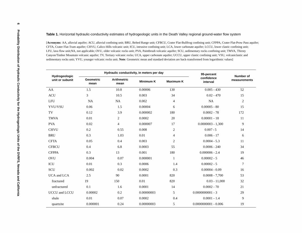
The logarithmically transformed values of hydraulic conductivity were used for statistical calcula-tions because this parameter tends to be normally dis-tributed (Neuman, 1982). The Cunnane plotting position method was used to assess the normality of the logarithms of hydraulic-conductivity measurements used for each HGU or HGU subcategory (Helsel and Hirsch, 1992, p. 27–29). The assumption of a normal distribution for log-transformed hydraulic conductivity was true. The probability plots for the combined upper and lower clastic confining units and the quartzites of the lower clastic confining unit were influenced by high outliers in the lower clastic confining unit. These data are from rare pumping tests, probably in highly frac-tured areas with enhanced permeability, and likely atypical. Field tests sample a greater volume of rock types than laboratory tests, thus, these results are more appropriate for application to a regional-scale numeri-cal model. The geometric and arithmetic means, range, and the 95-percent confidence intervals are listed in tables 1 and 2.

To compare the probability distributions of the log hydraulic conductivity for each HGU the data were normalized (Davis, 1986, p. 46–50). To compute the normalized values, the following equation (Davis, 1986, p. 48) was used:

,where Z is the normalized value, X is the observation (in this case log hydraulic

conductivity), X is the mean of the log-transformed observations

(or the geometric mean), and s is the standard deviation of the log-transformed

observations.The normalized values represent how many stan-

dard deviations particular values of log hydraulic con-ductivity are away from the geometric mean. The log hydraulic conductivities were plotted as a lognormal distribution by plotting the resulting distributions as a straight-line plot on log-probability coordinates. The distribution for the HGUs (and subcategories) was drawn using the spread plus or minus three standard deviations for log hydraulic-conductivity values reported for each HGU. These values correspond to the spread from 0.1 to 99.9 percentiles of the range of val-ues reported in Belcher and others (2001). The geomet-ric mean of the log hydraulic conductivity is at the

50-percentile value and the majority of the values were included in the range on either side of the mean (plus or minus two standard deviations).

Statistical Hypothesis Testing

Statistical hypothesis testing on the differences of the geometric means between the groupings of HGUs was performed. The large or small sample size with dif-fering variances test was used (as appropriate), with the level of significance being 0.05 (Mendenhall and Sin-ich, 1988, p. 376–378). The null hypothesis, that there is no difference between the geometric means, and the alternate corollary hypothesis, that a statistically signif-icant difference exists, were tested. The results of the hypothesis testing are listed in tables 3–9.

PROBABILITY DISTRIBUTIONS

Basin-Fill Hydrogeologic Units

The probability distributions of the hydraulic con-ductivity of the basin-fill hydrogeologic units are shown in figure 2. Units considered include: (1) a coarse, unconsolidated alluvial aquifer (AA), includes the older alluvial and younger alluvial aquifers (Belcher and others, 2001); (2) an alluvial confining unit (ACU) consisting predominantly of silt and clay playa deposits; and (3) undifferentiated basin filling of younger volcanic rocks (YVU) and Tertiary volcani-clastic and sedimentary rocks (VSU) are presented as combined data. The combined YVU/VSU unit shows a distinctly lower distribution of hydraulic conductivity than either the AA or the ACU (fig. 2). This result may be from the unconsolidated nature of the AA which gives it a greater hydraulic conductivity, coupled with a decrease in hydraulic conductivity of the older sedi-mentary and volcaniclastic rocks due to zeolitic alter-ation of the volcanic component. The hydraulic-conductivity values for the ACU are problematic, because these values generally are greater than those of the AA. This is probably an indication that the wells in which aquifer tests were performed may be from more permeable parts of the ACU. The ACU as defined by Belcher and others (2001) includes lacustrine carbon-ates that are locally productive aquifers (Dudley and Larson, 1976). The hypothesis testing confirms that the geometric mean of the ACU is similar to the AA and that the YVU/VSU unit is distinct from both the ACU and the AA (table 3).

Z X X–s

-------------=

PROBABILITY DISTRIBUTIONS 5

6 Pro

bab

ility Distrib

utio

n o

f Hyd

raulic C

on

du

ctivity for th

e Hyd

rog

eolo

gic U

nits o

f the D

VR

FS

, Nevad

a and

Califo

rnia

Table 1. Horizontal hydraulic-conductivity estimates of hydrogeologic units in the Death Valley regional ground-water flow system

[Acronyms: AA, alluvial aquifer; ACU, alluvial confining unit; BRU, Belted Range unit; CFBCU, Crater Flat-Bullfrog confining unit; CFPPA, Crater Flat-Prow Pass aquifer; CFTA, Crater Flat-Tram aquifer; CHVU, Calico Hills volcanic unit; ICU, intrusive confining unit; LCA, lower carbonate aquifer; LCCU, lower clastic confining unit; LFU, lava flow unit;NA, not applicable; OVU, older volcanic rocks unit; PVA, Paintbrush volcanic aquifer; SCU, sedimentary rocks confining unit; TMVA, Thirsty Canyon/Timber Mountain volcanic aquifer; TV, Tertiary volcanic rocks; UCA, upper carbonate aquifer; UCCU, upper clastic confining unit; VSU, volcaniclastic and sedimentary rocks unit; YVU, younger volcanic rocks unit. Note: Geometric mean and standard deviation are back-transformed from logarithmic values]

Hydrogeologic unit or subunit

Hydraulic conductivity, in meters per day 95-percent confidence

interval

Number of measurementsGeometric

meanArithmetric

meanMinimum K Maximum K

AA 1.5 10.8 0.00006 130 0.005 - 430 52

ACU 3 10.5 0.003 34 0.02 - 470 15

LFU NA NA 0.002 4 NA 2

YVU/VSU 0.06 1.5 0.00004 6 0.00005 - 80 15

TV 0.12 3.9 0.000002 180 0.0002 - 78 172

TMVA 0.01 2 0.0002 20 0.00001 - 18 11

PVA 0.02 4 0.000007 17 0.0000003 - 1,300 9

CHVU 0.2 0.55 0.008 2 0.007 - 5 14

BRU 0.3 1.03 0.01 4 0.006 - 17 6

CFTA 0.05 0.4 0.003 2 0.0004 - 5.3 11

CFBCU 0.4 6.8 0.0003 55 0.0006 - 240 34

CFPPA 0.3 13 0.001 180 0.000006 - 2.4 19

OVU 0.004 0.07 0.000001 1 0.00002 - 5 46

ICU 0.01 0.3 0.0006 1.4 0.00002 - 5 7

SCU 0.002 0.02 0.0002 0.3 0.00004 - 0.09 16

UCA and LCA 2.5 90 0.0001 820 0.0008 - 7,700 53

fractured 19 150 0.01 820 0.03 - 11,000 32

unfractured 0.1 1.6 0.0001 14 0.0002 - 70 21

UCCU and LCCU 0.00002 0.2 0.00000003 5 0.0000000001 - 3 29

shale 0.01 0.07 0.0002 0.4 0.0001 - 1.4 9

quartzite 0.000001 0.24 0.00000003 5 0.0000000001 - 0.006 19

PR

OB

AB

ILIT

Y D

IST

RIB

UT

ION

S 7

Table 2. Horizontal hydraulic-conductivity estimates of volcanic rock hydrogeologic units in the Death Valley regional ground-water flow system

[Geometric mean and standard deviation are back-transformed from logarithmic values]

Hydrogeologic unit or subunit

Hydraulic conductivity, in meters per day95-percent confidence

interval

Number of measurementsGeometric

meanArithmetric

meanMinimum K Maximum K

Lava flows 0.13 0.63 0.000007 4 0.0005 - 31 25

Ash-flow tuff 0.12 5.3 0.000002 180 0.0002 - 97 109

Non-welded to partially welded 0.06 6.6 0.0003 180 0.0002 - 24 43

Partially to moderately welded 0.04 1.1 0.000002 19 0.00003 - 50 35

Moderately to densely welded 1.6 13.3 0.02 55 0.005 - 540 7

Tuff breccia 0.31 4.2 0.0008 15 0.0002 - 550 11

Bedded tuff 0.14 2 0.00009 15 0.0003 - 57 14

Unaltered tuffs 0.4 8.1 0.00002 180 0.0006 - 260 71

Altered tuffs 0.04 1.3 0.000002 25 0.0001 - 15 63

8 Probability Distribution of Hy

-3

-2

-1

0

1

2

3

10-8 10-7 10-6 10-5 10-4 10-3 10-2 10-1 100 101 102 103 104 105

HYDRAULIC CONDUCTIVITY, IN METERS PER DAY

STA

ND

AR

D D

EV

IATO

NS

FR

OM

GE

OM

ET

RIC

ME

AN

Alluvial aquifer (AA)

Alluvial confining unit (ACU)

Younger volcanic unit and volcaniclastic sedimentary rocks unit (YVU/VSU)

0.005

0.01

0.05

0.1

0.25

0.5

0.025

0.75

0.9

0.95

0.975

0.9950.99

PE

RC

EN

T L

ES

S T

HA

N O

R E

QU

AL

TO

IND

ICA

TE

D V

ALU

E

Figure 2. Hydraulic-conductivity distributions for basin-fill hydrogeologic units.

Table 3. Results of hypothesis testing for basin-fill hydrogeologic units

[Acronyms: AA, alluvial aquifer; ACU, alluvial confining unit; VSU, volcaniclastic and sedimentary rocks unit; YVU, younger volcanic rocks unit. Abbreviations: NR, non-rejection of the null hypothesis; R, rejection of the null hypothesis. Note: Hydrogeologic units in column heading are being compared to those in row heading]

Null hypothesis:

Alternate hypothesis:

AA ACU YVU/VSU

AA -- NR R

ACU NR -- R

YVU/VSU NR R --

µ1 µ2– 0=

µ1 µ2– 0≠

draulic Conductivity for the Hydrogeologic Units of the DVRFS, Nevada and California

Bedrock Confining Hydrogeologic Units

Regional bedrock confining units include (1) a lower clastic confining unit (LCCU) of Late Protero-zoic through Lower Cambrian fine- to coarse-grained quartzite, siltstone, and conglomeratic sandstone; (2) an upper clastic confining unit (UCCU) consisting of Upper Devonian through Mississippian fine-grained clastic and carbonate rocks; (3) an intrusive confining unit (ICU) consisting of Cretaceous and Tertiary gra-nitic rocks; and (4) a sedimentary rock confining unit (SCU) consisting of Mesozoic cratonic sedimentary rocks (Winograd and Thordarson, 1975; Belcher and others, 2001). The thick, regionally distributed rocks of the LCCU show some of the lowest hydraulic-conduc-tivity measurements (fig. 3). As suggested by the hypothesis testing, the LCCU is distinct from the other confining units. The hydraulic conductivities of the UCCU, SCU, and ICU all have similar distributions (fig. 3), as confirmed by the hypothesis testing (table 4). Greater than expected hydraulic conductivities of the crystalline rocks of the ICU may be due to signifi-cant fracture permeability in these granites. Data for the distribution of the crystalline confining unit (XCU) were unavailable (Belcher and others, 2001).

Carbonate Rock Hydrogeologic Units

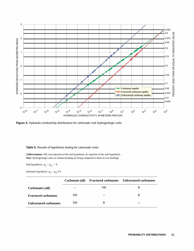
The distributions for the carbonate rocks, which form a regional aquifer in the DVRFS are shown in fig-ure 4. Outcrop and drill-hole observations and hydrau-lic-test data indicate that large hydraulic conductivities within the regional carbonate aquifer are often the result of secondary fracturing and dissolution (Wino-grad and Thordarson, 1975, p. C14–C30). Aquifer-test data from the carbonate rocks were subdivided and sta-tistically summarized to evaluate differences in hydrau-lic conductivity for rocks with extensive fracturing and rocks without extensive fracturing (fig. 4). These desig-nations were assessed from descriptions given on litho-logic logs from wells included in the aquifer tests (fig. 4). Extensive fracturing can increase hydraulic conduc-tivity values in the carbonate rocks. The hypothesis testing confirms that the geometric means of the frac-tured and unfractured carbonate are not equal; the dif-ferences between all carbonates and unfractured carbonates also are not equal (table 5).

Volcanic Rock Hydrogeologic Units

The Tertiary volcanic rocks were divided on the basis of lithostratigraphy (Sawyer and others, 1994; Slate and others, 2000) into the following units: Thirsty Canyon/Timber Mountain volcanic aquifer (TMVA), Paintbrush volcanic aquifer (PVA), Calico Hills volca-nic unit (CHVU), Wahmonie volcanic Unit (WVU), Belted Range unit (BRU), Crater Flat-Bullfrog confin-ing unit (CFBCU), Crater Flat-Prow Pass aquifer (CFPPA), Crater Flat-Tram aquifer (CFTA), and older volcanic unit (OVU). Each of these hydrogeologic units constitutes a variety of volcanic rocks with widely differing material properties such as lithology, degree of alteration, and degree of welding that vary both ver-tically and spatially (Blankennagel and Weir, 1973; Winograd and Thordarson, 1975). The hydraulic-con-ductivity distributions of these volcanic units overlap (fig. 5), as expected due to variations in lithology, alter-ation, and welding within individual HGUs. The hypothesis testing indicates that various units appear to have statistically significantly different geometric means while others are not statistically different (table 6). The WVU is not in figure 5 or in table 6, because no aquifer tests were reported for this unit (Belcher and others, 2001).

The Tertiary volcanic rocks were examined for the influence of lithology on hydraulic conductivity (table 2; fig. 6). Four lithologic groups were consid-ered: (1) ash-flow tuffs; (2) lava flows of rhyolite, rhy-odacite, and trachyte; (3) tuff breccia; and (4) bedded tuff. The distribution shown in figure 6 suggests that lithology of the Tertiary volcanic units, as defined in lithologic logs, is not an important factor for control-ling hydraulic conductivity. The hypothesis testing confirms that the geometric means are not statistically different between any of the lithologies of the Tertiary volcanic rocks (table 7).

Hydraulic-conductivity measurements for ash-flow tuffs were divided into three categories to assess the effect of welding (table 2) based on descriptions from borehole lithologic logs (Warren and others, 1998). These three categories are (1) non-welded to partially welded tuff; (2) partially to moderately welded tuff; and (3) moderately to densely welded tuff. Degrees of welding straddling these categories, such as non-welded to densely welded tuff, were omitted from this analysis. Descriptions of welding including only a single category were placed in the lower category (for example, all intervals described as “partially welded”



-3

-2

-1

0

1

2

3

10-8 10-7 10-6 10-5 10-4 10-3 10-2 10-1 100 101 102 103 104 105


STA

ND

AR

D D

EV

IAIT

ON

S F

RO

M G

EO

ME

TR

IC M

EA

N

Sedimentary rocks confining unit (SCU)

Intrusive confining unit (ICU)

Upper and lower clastic confining units (UCCU/LCCU)

Upper clastic confining unit (UCCU)–Shales

Lower clastic confining unit (LCCU)–Quartzites

0.9950.99

0.975

0.95

0.9

0.75

0.5

0.25

0.1

0.05

0.025

0.01

0.005

PE

RC

EN

T L

ES

S T

HA

N O

R E

QU

AL

TO

IND

ICA

TE

D V

ALU

E

Table 4. Results of hypothesis testing for bedrock confining units

[Acronyms: ICU, intrusive confining unit; LCCU, lower clastic confining unit; SCU,

sedimentary rocks confining unit; UCCU, upper clastic confining unit. Abbreviations:

NR, Non-rejection of null hypothesis; R, Rejection of null hypothesis; Note: Hydrogeologic units in column heading are being compared to those in row heading]

Null hypothesis:


SCU ICU UCCU/LCCU UCCU LCCU

SCU -- NR R NR R

ICU NR -- R NR R

UCCU/LCCU R R -- R R

UCCU NR NR R -- R

LCCU R R R R --

µ1 µ2– 0=

µ1 µ2– 0≠

Figure 3. Hydraulic-conductivity distributions for regional bedrock confining hydrogeologic units.


-3

-2

-1

0

1

2

3

10-8 10-7 10-6 10-5 10-4 10-3 10-2 10-1 100 101 102 103 104 105


STA

ND

AR

D D

EV

IAIT

ON

S F

RO

M G

EO

ME

TR

IC M

EA

N

Carbonate aquifer

Fractured carbonate aquifer

Unfractured carbonate aquifer

0.995

0.9

0.975

0.95

0.9

0.75

0.5

0.25

0.1

0.05

0.025

0.01

0.005

PE

RC

EN

T L

ES

S T

HA

N O

R E

QU

AL

TO

IND

ICA

TE

D V

ALU

E

Table 5. Results of hypothesis testing for carbonate rocks

[Abbreviations: NR, non-rejection of the null hypothesis; R, rejection of the null hypothesis. Note: Hydrogeologic units in column heading are being compared to those in row heading]

Null hypothesis:


Carbonate (all) Fractured carbonates Unfractured carbonates

Carbonates (all) -- NR R

Fractured carbonates NR -- R

Unfractured carbonates NR R --

µ1 µ2– 0=

µ1 µ2– 0≠

Figure 4. Hydraulic-conductivity distributions for carbonate rock hydrogeologic units.

-3

-2

-1

0

1

2

3

10-8 10-7 10-6 10-5 10-4 10-3 10-2 10-1 100 101 102 103 104 105


STA

ND

AR

D D

EV

IAIT

ON

S F

RO

M G

EO

ME

TR

IC M

EA

N

0.995

0.99

0.975

0.95

0.9

0.75

0.5

0.25

0.1

0.05

0.025

0.01

0.005

PE

RC

EN

T L

ES

S T

HA

N O

R E

QU

AL

TO

IND

ICA

TE

D V

ALU

E

Belted Range Unit (BRU)

Calico Hills volcanic unit (CHVU)

Paintbrush volcanic aquifer (PVA)

Thirsty Canyon/Timber Mountain volcanic aquifer (TMVA)

Crater Flat–Bullfrog confining unit (CFBCU)

Crater Flat–Prow Pass aquifer (CFPPA)

Crater Flat–Tram aquifer (CFTA)

Older volcanic rocks unit (OVU)

Table 6. Results of hypothesis testing for Tertiary volcanic rock hydrogeologic units

[Acronyms: BRU, Belted Range unit; CFBCU, Crater Flat-Bullfrog confining unit; CFPPA, Crater Flat-Prow Pass aquifer; CFTA, Crater Flat-Tram aquifer; CHVU, Calico Hills volcanic unit; OVU, older volcanic rocks unit; PVA, Paintbrush volcanic aquifer; TMVA, Thirsty Canyon/Timber Mountain volcanic

aquifer. Abbreviations: NR, non-rejection of null hypothesis; R, rejection of null hypothesis. Note: Hydrogeologic units in column heading are being compared to those in row heading]

Null hypothesis:


BRU CHVU PVA TMVA CFBCU CFPPA CFTA OVU

BRU --- NR NR R NR NR NR R

CHVU NR --- NR R NR NR NR R

PVA NR NR --- NR NR NR NR NR

TMVA R R NR --- R R NR NR

CFBCU NR NR NR R --- NR R R

CFPPA NR NR NR R NR --- NR R

CFTA NR NR NR NR R NR --- R

OVU R R NR NR R R R ---

µ1 µ2– 0=

µ1 µ2– 0≠

Figure 5. Hydraulic-conductivity distributions for Tertiary volcanic rock hydrogeologic units.


-3

-2

-1

0

1

2

3

10-8 10-7 10-6 10-5 10-4 10-3 10-2 10-1 100 101 102 103 104 105


0.995

0.99

0.975

0.95

0.9

0.75

0.5

0.25

0.1

0.05

0.025

0.01

0.005

STA

ND

AR

D D

EV

IAIT

ON

S F

RO

M G

EO

ME

TR

IC M

EA

N

PE

RC

EN

T L

ES

S T

HA

N O

R E

QU

AL

TO

IND

ICA

TE

D V

ALU

E

Ash-flow tuffs

Bedded tuffs

Lava flows

Tuff breccias

Figure 6. Hydraulic-conductivity distributions for Tertiary volcanic rock lithologies.

Table 7. Results of hypothesis testing for Tertiary volcanic rock lithologies

[Abbreviation: NR, non-rejection of the null hypothesis. Note: Hydrogeologic units in column heading are being compared to those in row heading]

Null hypothesis:


Ash-flow tuffs Bedded tuffs Lava flows Tuff breccias

Ash-flow tuffs -- NR NR NR

Bedded tuffs NR -- NR NR

Lava flows NR NR -- NR

Tuff breccias NR NR NR --

µ1 µ2– 0=

µ1 µ2– 0≠


only were included in the non-welded to partially welded tuff category). The hydraulic conductivity of ash-flow tuffs generally increases as the degree of welding increases (fig. 7). The non-welded to partially welded and the partially welded to moderately welded tuff categories appear to have lower overall values of hydraulic conductivity than the moderately welded to densely welded tuff category. The overlap of the hydraulic conductivity distributions for the two lesser-welded tuff groups may be an artifact of overlaps occurring in the reporting of the degree of welding present in the tested interval of the aquifer tests. Hypothesis testing confirms that the geometric means are not statistically different between the non-welded to partially welded and partially welded to moderately welded tuff categories, but that the geometric mean of the non-welded to partially welded and the partially welded to moderately welded tuff categories are statis-tically different from the moderately welded to densely welded tuff category (table 8).

Ash-flow tuffs, bedded tuffs, and tuff breccias were divided into two tuff categories, unaltered and altered (zeolitized or argillized), to assess the effect of alteration on hydraulic-conductivity measurements (table 2; fig. 8). Categorization was based on qualita-tive descriptions in borehole lithologic logs. Intervals of partly altered tuffs were omitted from this analysis. Clay minerals from the alteration of tuff tend to reduce permeability (Flint, 1998). The hydraulic conductivi-ties of altered ash-flow tuffs are less than those for the unaltered tuffs (fig. 8). The geometric mean of the hor-izontal hydraulic conductivity of the unaltered tuff is greater than altered tuff by about an order of magnitude (table 2). Hypothesis testing of the geometric mean confirms that the unaltered and altered tuffs are distinct from each other (table 9).

Applicability of Distributions to a Regional Model

Values of hydraulic conductivity and transmissiv-ity are dependent on the scale of the tests conducted to obtain these properties (Neuman, 1990). This scale effect generally is attributed to increasing access to a network of conduits for fluid flow as the volume of the medium encompassed by the test increases. In per-meameter tests of core samples done in the laboratory, the hydraulic conductivity of the rock matrix is deter-

mined, because these tests require unfractured core for successful results. Permeameter-test results generally are not useful for regional-scale ground-water flow models. Thus, results for permeameter tests of core samples are not utilized in the descriptive statistical calculations of the hydraulic parameters (with the exception of the LCCU). If a single-well aquifer test is of short duration, in a formation with low transmissiv-ity, or performed with minimal pumping rates, it typi-cally determines hydraulic properties, only in the near-borehole environment. The accuracy of these tests can be decreased by inefficient borehole construction, con-vergence of flow lines and related head losses as water flows into or out of sections of perforated casing, and head loss as water moves between the test-interval depth and the pump-intake depth. As such, transmissiv-ity estimates derived from single-well tests tend to be less than those of multiple-well tests. Storage-coeffi-cient estimates from single-hole tests have lesser reli-ability than those from multiple-well tests. Multiple-well aquifer tests manifest the influence of field-scale features, such as faults and fractures, as well as the water-transmitting properties of the rock matrix.

Because of these variables involving variously scaled tests, how to quantitatively scale the hydraulic-conductivity measurements among permeameter, slug, single-well, and multiple-well aquifer tests is currently unknown; only general comments can be made.

Principle of Parsimony

In the application of numerical flow model cali-bration, Hill (1998) introduces the concept of “parsi-mony.” The principle of parsimony (as applied to numerical models of ground-water flow) means to “start simple and add complexity as warranted by the hydrogeology and the inability of the model to repro-duce observations” (Hill, 1998, p. 35). The probability distributions presented in this report enable investiga-tors to apply the principle of parsimony. Both statistical hypothesis testing and visual examination of the prob-ability distributions indicate that several of the units in each category can be grouped together. The initial four groups of basin-fill units, bedrock confining units, car-bonate rock units, and volcanics represent an initial, practical grouping. Within these groups, the hypothesis testing and probability distributions provide further guidance for adding detail to the flow modeling if



-3

-2

-1

0

1

2

3

10-8 10-7 10-6 10-5 10-4 10-3 10-2 10-1 100 101 102 103 104 105


0.995

0.99

0.975

0.95

0.9

0.75

0.5

0.25

0.1

0.05

0.025

0.010.005

STA

ND

AR

D D

EV

IAT

ION

S F

RO

M G

EO

ME

TR

IC M

EA

N

PE

RC

EN

T L

ES

S T

HA

N O

R E

QU

AL

TO

IND

ICA

TE

D V

ALU

E

Ash-flow tuffs (all)

Non-welded to partially welded tuffs

Partially welded to moderately welded tuffs

Moderately welded to densely welded tuffs

Table 8. Results of hypothesis testing for welding in ash-flow tuffs

[Abbreviations: DW, densely welded; MW, moderately welded; NR, non-rejection of null hypothesis; NW; non-welded; PW, partially welded; R, rejection of null hypothesis. Note: Hydrogeologic units in column heading are being compared to those in row heading]

Null hypothesis:


NW/PW PW/MW MW/DW

NW/PW -- NR R

PW/MW NR -- R

MW/DW NR R --

µ1 µ2– 0=

µ1 µ2– 0≠

Figure 7. Hydraulic-conductivity distributions for welding in ash-flow tuffs.


-3

-2

-1

0

1

2

3

10-8 10-7 10-6 10-5 10-4 10-3 10-2 10-1 100 101 102 103 104 105


STA

ND

AR

D D

EV

IAT

ION

S F

RO

M G

EO

ME

TR

IC M

EA

N

0.9950.99

0.975

0.95

0.9

0.75

0.5

0.25

0.1

0.05

0.025

0.01

0.005

PE

RC

EN

T L

ES

S T

HA

N O

R E

QU

AL

TO

IND

ICA

TE

D V

ALU

E

Tuffs (all)

Unaltered tuffs

Altered tuffs

Table 9. Results of hypothesis testing for alteration in tuffs

[Abbreviation: R, rejection of null hypothesis. Note: Hydrogeologic units in column heading are being compared to those in row heading]

Null hypothesis:


Tuffs (all) Unaltered Altered

Tuffs (all) -- R R

Unaltered R -- R

Altered R R --

µ1 µ2– 0=

µ1 µ2– 0≠

Figure 8. Hydraulic-conductivity distributions for alteration in ash-flow tuffs.

required during calibration. Within the basin-fill units, the AA and the ACU are similar enough that they ini-tially could be considered the same unit, with the YVU/VSU being distinct. Within the bedrock confin-ing units, the UCCU and the ICU could be combined and the LCCU would exist as a separate unit. Fractured and unfractured carbonates appear to be distinct from one another and could be separated on that basis. The hydrogeologic units of the Tertiary volcanic rocks could be divided into three separate units: (1) TMVA and PVA; (2) BRU, CFBCU, CFPPA, and CFTA; and (3) CHVU and WVU (although no aquifer test data for the WVU exist, it is geologically similar to the CHVU). Alteration of all tuffs and welding in the ash-flow tuffs also appears to be a mechanism for adding complexity to a numerical model.

SUMMARY

The probability distributions of hydraulic con-ductivity were estimated to support regional-scale sim-ulation of ground-water flow in the Death Valley regional ground-water flow system. Fracturing appears to have the greatest influence on the permeability of bedrock hydrogeologic units, within this region. The degree of alteration and welding in the Tertiary volca-nic rocks also influences hydraulic conductivity. As the degree of alteration increases, hydraulic conductivity decreases. Increasing welding appears to increase hydraulic conductivity because degrees of welding increases the brittleness of the volcanic rocks, thus increasing the amount of fracturing.

Probability distributions can be used to apply the principle of parsimony for combining hydrogeologic units. Visual examination of the probability distribu-tions and the use of statistical hypothesis testing allows groupings of the hydrogeologic units to be made, gen-eralizing the units contained within a ground-water flow model. If warranted, complexity can be made by dividing units, either along hydraulic properties (for example welding or alteration in tuffs) or hydrogeo-logic units.

The hydraulic-conductivity distributions pre-sented in this report have a greater use beyond that associated with the regional ground-water flow model being developed by the USGS. The probability of hydraulic-conductivity distributions could be used for many purposes including contaminant-transport mod-eling, water-supply issues, and resource protection. The distributions also could be used for similar rock

types in areas outside of the southern Great Basin because volcanics, carbonates, and clastics rock types that were analyzed occur worldwide.

REFERENCES CITED

Bedinger, M.S., Langer, W.H., and Reed, J.E., 1989, Hydraulic properties of rocks in the Basin and Range province, in Bedinger, M.S., Sargent, K.A., Langer, W.H., Sherman, F.B., Reed, J.E., and Brady, B.T., Stud-ies of geology and hydrology in the Basin and Range province, southwestern United States, for isolation of high-level radioactive waste — Basis of characteriza-tion and evaluation: U.S. Geological Survey Profes-sional Paper 1370-A, p. 16–18.

Belcher, W.R., Elliott, P.E., and Geldon, A.L., 2001, Hydrau-lic-property estimates for use with a transient ground-water flow model for the Death Valley regional ground-water flow system, Nevada and California: U.S. Geo-logical Survey Water-Resources Investigations Report 01-4210, 33 p., last accessed 8/5/2002 at URL http://water.usgs.gov/pubs/wri/wri014210/.

Blankennagel, R.K., and Weir, J.E., Jr., 1973, Geohydrology of the eastern part of Pahute Mesa, Nevada Test Site, Nye County, Nevada: U.S. Geological Survey Profes-sional Paper 712-B, 35 p.

D'Agnese, F.A., Faunt, C.C., Turner, A.K., and Hill, M.C., 1997, Hydrogeologic evaluation and numerical simula-tion of the Death Valley regional ground-water flow system, Nevada and California: U.S. Geological Survey Water-Resources Investigations Report 96-4300, 124 p.

D’Agnese F.A., Faunt, C.C., Hill, M.C., and Turner, A.K., 1999, Death Valley regional ground-water flow model calibration using optimal parameter estimation methods and geoscientific information systems: Advances in Water Resources, v. 22, p. 777–790.

Davis, J.C., 1986, Statistics and data analysis in geology, 2d ed.: New York, John Wiley and Sons, 64 p.

Dettinger, M.D., 1989, Distribution of carbonate-rock aqui-fers in southern Nevada and the potential for their development—Summary of findings: Carson City, Nev., 1985–88, Program for the Study and Testing of Carbonate-Rock Aquifers in Eastern and Southern Nevada, Summary Report No. 1, 37 p.

Dudley, W.W., Jr., and Larsen, J.D., 1976, Effect of irrigation pumping on desert pupfish habitats in Ash Meadows, Nye County, Nevada:. U.S. Geological Survey Profes-sional Paper 927, 52 p.

Faunt, C.C., 1997, Effect of faulting on ground-water move-ment in the Death Valley region, Nevada and California: U.S. Geological Survey Water-Resources Investiga-tions Report 95-4132, 42 p.

SUMMARY 17

Flint, L.E, 1998, Characterization of hydrogeologic units using matrix properties, Yucca Mountain, Nevada: U.S. Geological Survey Water-Resources Investigations Report 97-4243, 64 p.

Freund, J.E., 1992, Mathematical statistics, 5th ed.: Engle-wood Cliffs, New Jersey, Prentice-Hall, 658 p.

Grose, T.L.T., and Smith, G.I., 1989, Geology, in Bedinger, M.S., Sargent, K.A., and Langer, W.H., eds., Studies of geology and hydrology in the Basin and Range Prov-ince, southwestern United States, for isolation of high-level radioactive waste—Characterization of the Death Valley Region, Nevada and California: U.S. Geo-logical Survey Professional Paper 1370-F, p. F5–F19.

Helsel, D.R., and Hirsch, R.M., 1992, Statistical methods in water resources: Amsterdam, The Netherlands, Elsevier, 529 p.

Hill, M.C., 1998, Methods and guidelines for effective model calibration: U.S. Geological Survey Water-Resources Investigations Report 98-4005, 90 p.

Laczniak, R.J., Cole, J.C., Sawyer, D.A., and Trudeau, D.A., 1996, Summary of hydrogeologic controls on ground-water flow at the Nevada Test Site, Nye County, Nevada: U.S. Geological Survey Water-Resources Investigations Report 96-4109, 59 p.

Mendenhall, William, and Sinich, Terry, 1988, Statistics for the engineering and computer sciences, 2nd ed.: San Francisco, California, Dellen Publishing Co., 1036 p.

Mifflin, M.D., 1988, Region 4, Great Basin, in Back, W., Rosenshein, J.S., and Seaber, P.R., eds., Hydrogeology, The geology of North America, v. O-2: Boulder, Colo-rado: Geological Society of America, p. 69–78.

Neuman, S.P., 1982, Statistical characterization of aquifer heterogeneities: an overview, in Narasimhan, T.N., ed., Recent trends in hydrogeology: Boulder, Colo., Geo-logical Society of America Special Paper 189, p. 81–102.

–––––1990, Universal scaling of hydraulic conductivities and dispersivities in geologic media: American Geo-physical Union, Water Resources Research, v. 26, no. 8, p. 1749–1758.

Plume, R.W., 1996, Hydrogeologic framework of the Great Basin region of Nevada, Utah, and adjacent states: U.S. Geological Survey Professional Paper 1409-B, 64 p.

Prudic, D.E., Harrill, J.R., and Burbey, T.J., 1995, Concep-tual evaluation of regional ground-water flow in the car-bonate-rock province of the Great Basin, Nevada, Utah, and adjacent states: U.S. Geological Survey Profes-sional Paper 1409-D, 102 p.

Sawyer, D.A., Fleck, R.J., Lanphere, M.A., Warren, R.G., Broxton, D.E., and Hudson, M.R., 1994, Episodic caldera volcanism in the Miocene southwestern Nevada volcanic field: revised stratigraphic framework, 40Ar/39Ar geochronology, and implications for magma-tism and extension: Geological Society of America Bulletin, v. 106, p.1304–1318.

Slate, J.L, Berry, M.E., Rowley, P.D., Fridrich, C.J., Morgan, K.S., Workman, J.B., Young, O.D., Dixon, G.L., Will-iams, V.S., McKee, E.H., Ponce, D.A., Hildenbrand, T.G., Swadley, WC, Lundstrom, S.C., Ekren, E.B., Warren, R.G., Cole, J.C., Fleck, R.J., Lanphere, M.A., Sawyer, D.A., Minor, S.A., Grunwald, D.J., Laczniak, R.J., Menges, C.M., Yount, J.C., and Jayko, A.S., 2000, Digital geologic map of the Nevada Test Site and vicin-ity, Nye, Lincoln, and Clark Counties, Nevada, and Inyo County, California: U.S. Geological Survey Open-File Report 99-554A, 53 p., scale 1:120,000.

Stewart, J.H., 1978, Basin and range structure in North America - a review, in Smith, R.B., and Eaton, G.P., eds., Cenozoic tectonics and regional geophysics in the western Cordillera, Memoir 152: Geological Society of America, Boulder, Colorado, p. 1–31.

U.S. Department of Energy, 1997, Regional groundwater flow and tritium transport modeling and risk assessment of the Underground Test Area, Nevada Test Site, Nevada: U.S. Department of Energy Report DOE/NV-477 (Underground Test Area subproject, Phase I data analysis task, v. VI, Groundwater flow model data doc-umentation package, ITLV/10972-181), various pagination.

Warren, R.G., Sawyer, D.A., Byers, Jr., F.M, and Cole, J.C., 1998, A petrographic/geochemical database and strati-graphic and structural framework of the Southwestern Nevada Volcanic Field: U.S. Department of Commerce, National Oceanic and Atmospheric Administration, National Geophysical Data Center, last accessed March 7, 2001, at URL: <http://queeg.ngdc.noaa.gov/seg/geochem/swnvf/>.

Winograd, I.J., and Thordarson, William, 1975, Hydrogeo-logic and hydrochemical framework, south-central Great Basin, Nevada-California, with special reference to the Nevada Test Site: U.S. Geological Survey Profes-sional Paper 712-C, 126 p.


Probability Distributions of Hydraulic Conductivity for ... · Probability Distributions of...

Documents

Transcript of Probability Distributions of Hydraulic Conductivity for ... · Probability Distributions of...