11.5 Economic Applications of the Derivative

Question 1: What does the term marginal mean?

Question 2: How are derivatives used to compute elasticity?

Derivatives are perfect for examining change. By their definition, they tells us how one

variable changes when another variable changes. In business and economics, this

allows us to examine how revenue and cost change as the quantity produced and sold

changes. Marginal revenue and marginal cost help a business determine compute

these changes.

Elasticity is used to determine how changes in price affect the quantity demanded by

consumers. Understanding this relationship helps us to determine whether a price

should be increased or decreased.

In this section we’ll examine these terms and apply them to several examples drawn

from businesses operating in the real world.

1

Question 1: What does the term marginal mean?

In economics, the term marginal is used to indicate the change in some benefit or cost

when an additional unit is produced. For instance, the marginal revenue is the change in

total revenue when an additional unit is produced. If we let the total revenue function be

represented by TR Q , where Q is the number of units produced and sold, then the

marginal revenue is calculated with the difference

Marginal Revenue 1TR Q TR Q

Since this is a difference, it corresponds to a change in revenue. The production levels

Q and 1Q differ by one units, so 1TR Q TR Q describes the change in total

revenue when production is changed by one unit.

The marginal revenue can also be interpreted as an average rate of change. Using the

definition of average rate of change, the average rate of change of R Q over , 1Q Q

is

Average rate of change 1

of over , 1

TR Q TR Q

T Q QR Q Q

1 Q 1TR Q TR Q

Let’s label these quantities on a graph of a revenue function ( )TR Q .

2

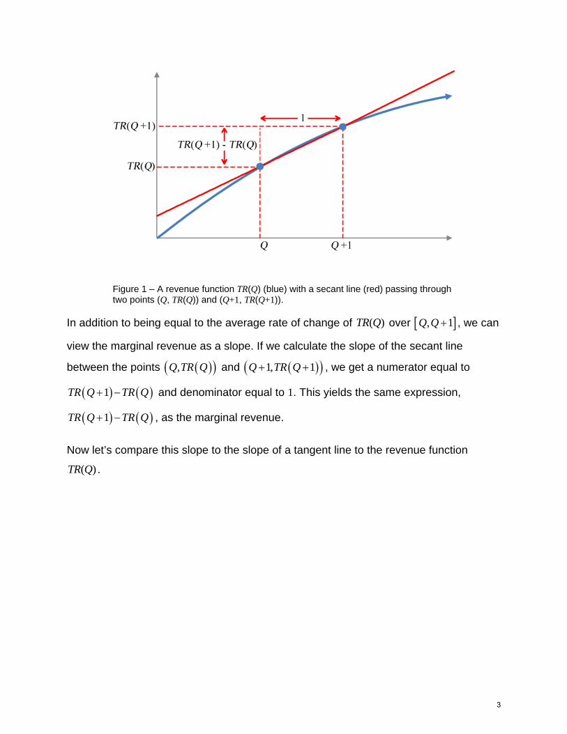
Figure 1 – A revenue function TR(Q) (blue) with a secant line (red) passing through two points (Q, TR(Q)) and (Q+1, TR(Q+1)).

In addition to being equal to the average rate of change of ( )TR Q over , 1Q Q , we can

view the marginal revenue as a slope. If we calculate the slope of the secant line

between the points ,Q TR Q and 1, 1Q TR Q , we get a numerator equal to

1TR Q TR Q and denominator equal to 1. This yields the same expression,

1TR Q TR Q , as the marginal revenue.

Now let’s compare this slope to the slope of a tangent line to the revenue function

( )TR Q .

3

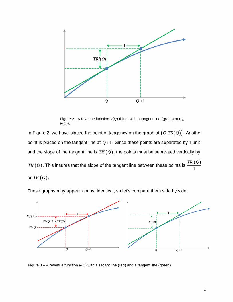
Figure 2 - A revenue function R(Q) (blue) with a tangent line (green) at (Q, R(Q)).

In Figure 2, we have placed the point of tangency on the graph at ,Q TR Q . Another

point is placed on the tangent line at 1Q . Since these points are separated by 1 unit

and the slope of the tangent line is TR Q , the points must be separated vertically by

TR Q . This insures that the slope of the tangent line between these points is 1

TR Q

or TR Q .

These graphs may appear almost identical, so let’s compare them side by side.

Figure 3 – A revenue function R(Q) with a secant line (red) and a tangent line (green).

4

The secant line (red) and the tangent line (green) both pass through ,Q TR Q .

However, the tangent line is slightly steeper and passes through a slightly higher point

than the secant line. This means the slope of the tangent line is approximately the same

as the slope of the secant line. In terms of the revenue,

Slope of the secant line Slope of the tangent line

1

1 1

TR Q TR Q TR Q

 

The marginal revenue at a production level Q is

approximately equal to the derivative of the total revenue

function at Q,

1TR Q TR Q TR Q

We can evaluate the derivative of the revenue function to estimate the marginal revenue

at any production level.

Example 1 Find and Interpret the Marginal Revenue

Based on sales data from 2000 to 2009, the relationship between the

price per barrel of beer P at the Boston Beer Company and the number

of barrels sold annually, Q, can be modeled by the power function

0.0209209.7204P Q

where Q is in thousands of barrels.

5

a. Find the revenue function ( )TR Q .

Solution To find the revenue, we must multiply the quantity times the

price. In this example, the quantity of beer is represented by Q in

thousands of barrels and the price per barrel is reprensented by

0.0209209.7204P Q in dollars per barrel. The revenue function is

0.0209

quantity price

( ) 209.7204TR Q Q Q

Simplifying the function by combining the factors,

0.9791209.7204TR Q Q

where the exponents have been added on the Q factors.

The units of the revenue function are very important. By multiplying the

units on the price and the quantity, we can determine the units on the

revenue function:

units on units onthousands of

the quantity the prbarrels

ice

dollars

barrel

thousands of dollars

We complete the total revenue function by labeling the units on the

function and write

0.9791209.7204 thousand dollarsTR Q Q

b. Find the annual revenue when 1,500,000 barrels of beer are sold.

Solution The annual revenue from 1,500,000 barrels of beer is found by

substituting this production level into ( )R Q . Since Q is in thousands of

barrels, we need to divide the production level by 1000 to scale it

properly,

6

1,500,000 barrels 1 thousand barrels

1 1000 bar rels 1500 thousand barrels

The conversion factor, 1 thousand barrels

1000 barrels, is equal to 1 and converts

1,500,000 barrels to 1500 thousand barrels. The revenue at this product

level is

0.9791(1500) 209.7204 1500 269,992.4558 thousand dollarsTR

We can convert this amount to dollars by multiplying by 1000,

thou269, sand992.4558 dol lars

t

1000 dollars

1 housand do1 llars 269,992, 455.8 dollars

c. Approximate the marginal revenue when 1,500,000 barrels of beer

are sold.

Solution The marginal revenue at 1,500,000 barrels of beer is

approximated by (1500)TR . We can find the derivative using the power

rule for derivatives,

0.9791

0.9791

.0209

0.0209

( ) 209.7204

209.7204

209.7204 0.9791

205.3372

dTR Q Q

dQ

dQ

dQ

Q

Q

The marginal revenue is approximately

0.0209(1500) 205.3372 1500 176.2330TR

Use the Constant Times a Function Rule

Use the Power Rule

Multiply the constants

7

d. How will revenue change if production is increased from 1,500,000

barrels?

Solution The marginal revenue is the same as the instantaneous rate of

change and has the same units. These units are found by dividing the

units on the dependent variable by the units on the independent

variable,

units on the dependent variable thousand

units on the independent variable

dollars

thousand

dollars

barrels barrels

The marginal revenue is about 176.2330 dollars per barrel meaning that

an increase in production of one barrel will result in an increase in

revenue of approximately 176.23 dollars.

The actual increase is found by subtract the revenue at each level,

0.9791 0.9791(1500.001) (1500) 209.7204 1500.001 209.7204 1500

0.17623309 thousand dollars

TR TR

or 176.23309 dollars.

The marginal cost is the change in cost when an additional unit is produced. If Q units

are produced at a total cost ( )TC Q , the marginal cost is defined as

Marginal Cost 1TC Q TC Q

This definition is identical to the definition of marginal revenue except that the total cost

function is used instead of the total revenue function. Like the marginal revenue, the

marginal cost at a production level Q is approximately the same as the derivative of the

total cost function.

8

The marginal cost at a production level Q is approximately

equal to the derivative of the total cost function at Q,

1TC Q TC Q TC Q

Example 2 Find and Interpret the Marginal Cost

The total cost TC Q to produce Q thousand barrels of beer at the Craft

Brewers Alliance from 2000 to 2009 is given by the function

3 2( ) 0.0024 2.9978 961.4000 119249.2929TC Q Q Q Q

where the cost is in thousands of dollars.

a. Approximate the marginal cost for a production level of 300,000

barrels of beer.

Solution The marginal cost at a production level of 300,000 barrels of

beer is approximated by ( )TC Q at that production level. The derivative

of the cost function is

3 2

2

2

( ) 0.0024 2.9978 961.4000 119249.2929

0.0024 3 2.9978 2 961.400 1 0

0.0072 5.9956 961.4000

dTC Q Q Q Q

dQ

Q Q

Q Q

Since the quantity Q is in thousands of barrels, we must substitute 300

thousand into ( )TC Q to estimate the marginal revenue at 300,000

barrels. When we do this, we get

2(300) 0.0072 300 5.9956 300 961.4000

189.28

TC

9

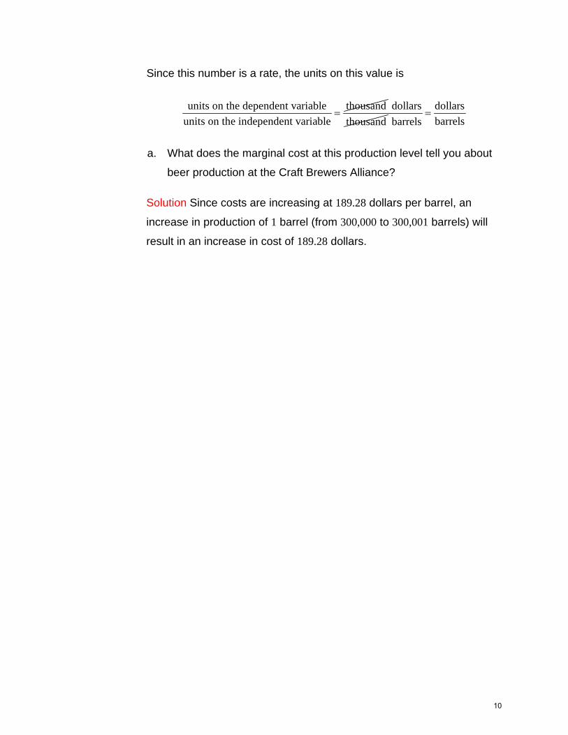
Since this number is a rate, the units on this value is

units on the dependent variable thousand

units on the independent variable

dollars

thousand

dollars

barrels barrels

a. What does the marginal cost at this production level tell you about

beer production at the Craft Brewers Alliance?

Solution Since costs are increasing at 189.28 dollars per barrel, an

increase in production of 1 barrel (from 300,000 to 300,001 barrels) will

result in an increase in cost of 189.28 dollars.

10

Question 2: How are derivatives used to compute elasticity?

In economics, the term elasticity refers to the responsiveness of one economic variable

to changes in another economic variable. The elasticity is measured in terms of

percentage changes instead of absolute changes. This means we measure the change

in a variable as a percentage of the original amount of the variable. For instance, the

percent change in a variable X is defined as

Change in the variable Percent change in

Original value of

XX

X

This definition can be symbolized in a compact form by symbolizing the change as ∆ X.

If a variable X changes from one value X to another value X

+ ∆X, then

Percent change in X

XX

Suppose that the value of X changes from 20 to 30. The percentage change is

30 20Percent change in 0.5

20X

Written as a percentage, this is a percentage change in X of 50%.

If we wish to find the elasticity of Y with respect to X, we find the ratio of the percentage

change in Y to the percentage change in X.

The elasticity of Y with respect to X is

Percent change in Elasticity of with respect to

Percent change in

YY X

X

11

For most elasticity calculations, the percent change in one variable corresponds to an

increase while the other percent change corresponds to a decrease. This means the

numerator and denominator will have opposite signs resulting in a negative value. Some

textbooks will define the elasticity with a negative sign or in absolute values, but we’ll

preserve the sign to emphasize the nature of the percent changes. An elasticity more

negative than -1 indicates that a percent increase in X corresponds to a greater percent

decrease in Y. In this case, we would say that the variable Y is elastic with respect to

variable X.

An elasticity between -1 and 0 indicates that a percent increase in X corresponds to a

smaller percent decrease in Y. In this case, the variable Y is inelastic with respect to the

variable X.

An elasticity of -1 means that a percent increase in X corresponds to an identical

percent decrease in the variable Y. In this case, the variable Y is said to be unit-elastic

with respect to the variable X.

The most common use of elasticity in economics is price elasticity of demand or

elasticity of demand with respect to price. This concept allows us to explore the

responsiveness of the consumer demand for some product or service to changes in the

price of that product or service. If the price of a cup of coffee were to increase, how

would this effect the quantity sold? In 2006, Starbuck’s increased prices on all coffee

drinks by 5 cents. At one franchise in Sacramento, California, the price on a tall coffee

increased from $1.65 to $1.70. As expected, the demand for tall coffees dropped from

440 units per day to 436 units per day. The percent change in price P is

1.70 1.65.03

1.65

P

P

or about 3%. The percent change in the demand Q is

436 440.009

440

Q

Q

12

or about -0.9%. An 3% increase in price corresponds to a 0.9% decrease in the quantity

of tall coffees sold.

The elasticity of demand with respect to price or price elasticity of demand is

Percent change in 0.0090.3

Percent change in P .03

QE

Since this is a ratio, we can think of it as 0.3

1

and say that a 1% increase in price

corresponds to a 0.3% drop in demand for tall coffee. On the other hand, we could also

think of this ratio as 0.3

1 and say that a 1% drop in price corresponds to a 0.3% increase

in demand. Many economics textbooks work in terms of larger price changes and will

interpret this ratio as 3

10

. In this case, we would say that a 10% increase in the price of

a tall coffee is accompanied by a 3% decrease in demand.

If the relationship between demand and price is given by a function, we can utilize the

derivative of the demand function to calculate the price elasticity of demand. If we write

think of the change in price as being from P to P P and the corresponding change in

demand as being from Q to Q Q , the corresponding percent changes in price and

demand are P

P

and

Q

Q

. The definition of elasticity leads to

Percent change in

Percent change in P

QE

QQP

P

Q P

Q P

P Q

Q P

Definition of price elasticity of demand

Replace the percent changes with appropriate symbols

Dividing by P

P

is the same as

multiplying by the reciprocal PP

Rearrange the factors in the numerators of each fraction.

13

The factor Q

P

represents the average rate of change of demand Q with respect to

price P. If we assume the change in price is small, we can replace the average rate of

change with the instantaneous rate of change, dQ

dP.

If the demand Q and the price P are related by a demand

function ( )Q f P , then the price elasticity of demand E is

EP dQ

Q dP

If 1E , then demand is elastic and a percent increase in

price yields a larger percent decrease in demand.

If 1 0E , then demand is inelastic and a percent

increase in price yields a smaller percent decrease in

demand.

Several other cases of elasticity should be mentioned. If 1E , then the demand is

unit-elastic and a percent increase in price yields the same percent decrease in

demand. Demand is perfectly elastic if any increase in price causes the quantity

demanded to decrease to 0. Demand is perfectly inelastic if and increase or decrease in

price makes no change in the quantity demanded.

Some economists prefer to define elasticity as a positive number by taking the absolute

value of P dP

Q dQ . This change loses the idea that an increase in price leads to a drop in

the quantity sold, For this reason, we’ll use the definition above for computing price

elasticity of demand.

14

Example 3 Calculate the Price Elasticity of Demand

Using data from market years 2000 through 2010, the relationship

between the price per bushel of oats and the number of bushels of oats

sold is given by

0.543152.07Q P

where P is in dollars and Q is in millions of bushels.

a. Find the price elasticity of demand when the price per bushel is

$1.75.

Solution Since the relationship between the quantity and price is given

as a function of price, we may compute the price elasticity of demand

from

P dQE

Q dP

The derivative dQ

dP is found from the relationship between quantity and

price. Using the Product with a Constant Rule and the Power Rule, we

get

0.543

1.543

1.543

152.07

152.07 0.543

82.574

dQ dP

dP dP

P

P

Substitute the expression 1.54382.574dQ

PdP

for the derivative and the

quantity 0.543152.07Q P into the elasticity formula yields

15

1.5430.543

82.574152.07

0.543

P dQE

Q dP

PP

P

Since the elasticity simplifies to a form that does not contain P, the

elasticity does not depend upon price.

b. Is the demand for oats elastic or inelastic when the price per bushel

is $1.75?

Solution Since the elasticity, 0.543E , is between -1 and 0, the

elasticity is inelastic. As a consequence, a change in price of 1% will

result in a 0.543% decrease in the quantity demanded.

The product of the price per unit and the quantity demanded is equal to the revenue

from the product. If the quantity demanded decreases as the price is increased, what

will be the overall effect on the total revenue? To answer this question, let’s examine a

table of prices, corresponding quantities, revenue and the elasticity for a product where

the demand function is 120Q P .

price P 20 40 60 80 100

quantity Q 100 80 60 40 20

total revenue TR 2000 3200 3600 3200 2000

price elasticity of demand E

-0.2 -0.5 -1 -2 -5

Even though the slope of the demand curve is -1, the price elasticity of demand

changes as the price increases. For lower prices (green), the price elasticity of demand

is between -1 and 0 and increasing the price increases revenue. For higher prices

16

(blue), the elasticity is more negative than 1 and increasing the price leads to lower

revenue. The highest revenue occurs when the elasticity is equal to -1.

Should prices be increased?

1. If demand is inelastic 1 0E , then a price increase

yields an increase in total revenue.

2. If demand is elastic 1E , then a price increase yields

a decrease in total revenue.

3. Total revenue is highest at a price where demand is unit-

elastic.

For inelastic demand, price increases are countered by small decreases in the quantity

resulting in more revenue. However, when demand is elastic, price increases lead to

large drops in the quantity sold that lowers the overall revenue. If maximizing revenue is

the overall goal, setting the price where the price elasticity of demand is equal to -1 is

ideal. This goal ignores cost and should be approached cautiously.

Example 4 Calculate the Price Elasticity of Demand

A small technology company in Northern California is developing a

tablet PC to compete with Apple’s Ipad. Based on market surveys, the

company believes the quantity Q (in thousands of units) that will be

demanded by consumers is related to the price P (in thousands of

dollars) by the relationship

24000 250Q P

17

a. Find the price elasticity of demand when the price of the tablet PC

is $3000.

Solution To compute the price elasticity of demand, we need to find the

derivative of the demand function 24000 250Q P :

2

2

4000 250

4000 250

0 250 2

500

dQ dP

dP dP

d dP

dP dP

P

P

Use the derivative and the expression for the quantity Q in the formula

for price elasticity of demand,

2500

4000 250

P dQE

Q dP

PP

P

We can simplify the right hand side of this equation to make it easier to

substitute the price in:

2

2

2

500

4000 250

500

4000 250

P PE

P

P

P

A tablet PC priced at 3000 dollars corresponds to 3P . If we put this

value into the expression for price elasticity of demand, we get

2

2

500 32.57

4000 250 3E

Use the Sum / Difference Rule and the Constant Times a Function Rule

Use the Power Rule

Combine factors

Simplify numerator

18

Since the elasticity, 2.57E , is more negative than -1, the demand is

elastic. As a consequence, revenue will drop as the price increases.

b. At what price is the price elasticity of demand equal to -1?

Solution From part a, we know that a price of $3000 is elastic. At lower

prices the demand might be inelastic. To find the dividing line between

elastic and inelastic, we set the price elasticity of demand equal to -1,

2

2

5001

4000 250

P

P

Now solve for P:

2

2 22

2 2

2

2

5004000 250 1 4000 250

4000 250

500 4000 250

750 4000

16

3

16

3

PP P

P

P P

P

P

P

The negative price is not a possible value for the price of a tablet PC.

The other price, 163P , is approximately 2.309. Since P has units of

thousands of dollars, this value corresponds to a price of $2309.

Multiply both sides by the denominator to clear fraction

Add 250P2 to both sides

Divide both sides by 750 and reduce

Square root both sides of the equation

19

Figure 4 – At the point of intersection, the elasticity is equal to -1. To the left or right of the point of intersection, the price elasticity of demand is either lower or higher than -1.

If the price is lower than $2309, the value of E is lower than -1 meaning

demand is inelastic. Prices higher than $2309 result in elastic demand.

This means revenue is maximized at a price of $2309.

(P,E ) (2.309, -1)

20