1. Second Order ODEs andSturm-Liouville theory

1.1 General 2nd Order ODEs

Arfken 7.4

(Riley 15.0,15.2)

1.1.1 Introduction

Consider a general linear second order differential equation:1

p0(x)y′′(x) + p1(x)y′(x) + q(x)y(x) = f(x). (1.1)

It is linear because each term on the LHS contains only y, y′ or y′′, not for instance y2 or yy′.The functions p0, p1, q, and f are assumed to be given and may be complex (but usually arereal), and we want to find y. Usually the functions are defined on a given range a ≤ x ≤ b.

We often write this schematically as

Ly(x) = f(x),

where L is a differential operator that acts on one function to produce another.The space of functions we will be interested in is that of complex functions of the real

variable x which are square-integrable on the interval x ∈ [a, b], denoted L2[a, b]. These forma vector space with an inner product (a Hilbert space). We will usually require them to beat least twice differentiable, except possibly at isolated points, and will not constantly refer tosuch restrictions.

If f(x) 6= 0 the equation is inhomogeneous; if f(x) = 0 the equation is homogeneous:

p0(x)y′′(x) + p1(x)y′(x) + q(x)y(x) = 0. (1.2)

Linearity implies that if y1 and y2 are both solutions of the homogeneous equation, then so isAy1 +By2 for (complex) constants A and B.

Often we divide (1.1) by p0(x) to get the alternate form of the equation

y′′(x) + P (x)y′(x) +Q(x)y(x) = F (x). (1.3)

or for the homogeneous case

y′′(x) + P (x)y′(x) +Q(x)y(x) = 0. (1.4)

1Most of the time after this introductory section we will be concerned with problems in which p′0 = p1, inwhich case we will denote p0 and q0 by −p and q.

1

At most values of x, P (x) and Q(x) are finite; such points are ordinary points of the equation.If, at some point x = x0, P (x) or Q(x) diverges, but (x − x0)P (x) and (x − x0)

2Q(x) arefinite, x0 is called a regular singular point. If P (x) diverges faster than 1/(x− x0) and/or Q(x)diverges faster than 1/(x− x0)2 we speak of an irregular singular point. The relevance of thisclassification for the solutions is as follows: at an ordinary point solutions are analytic andhave Taylor expansions with a radius of convergence governed by the distance to the nearestsingular point in the complex plane. At a regular singular point a solution may be analyticor at worst will have a pole or a branch point; at least one solution will exist of the formy(x) = (x−x0)su(x) where u(x) is analytic and s is a number called the indicial exponent. Wewill meet this again when we seek series solutions of common differential equations.

1.1.2 Linear independence and second solutions

It is useful to have a way to check if a set of n functions {ui(x)} are linearly independent. Bydefinition if they not, we can find a set of coefficients ci, not all zero, such that for all x inthe range

∑ni ciui(x) = 0. Assuming the functions to be differentiable at least n− 1 times, we

can obtain further equations for the coefficients by differentiating this equation multiple times;writing the mth derivative of ui as u

(m)i , we have

u1 u2 . . . unu′1 u′2 . . . u′n...

......

......

...

u(n−1)1 u

(n−1)2 . . . u

(n−1)n

c1c2

...cn

= 0

For any given x this is just a matrix equation, and it can only hold, for ci not all zero, if thedeterminant of the matrix vanishes. This determinant is called the Wronskian of the functions(the “W” is silent).

So if a set of functions is not linearly independent over a range, their Wronskian vanishesfor all x in the range. The converse is true also true in all cases of interest to us: a vanishingWronskian implies linear dependence. Linearly-independent functions will have a Wronskianwhich does not vanish (except possibly at isolated points).

The Wronskian allows us to determine that there are at most two independent solutionsof a homogeneous 2nd order equation. Consider three solutions of the homogeneous equation(1.4), y1, y2 and y3. Then

W (x) =

∣∣∣∣∣∣y1 y2 y3y′1 y′2 y′3y′′1 y′′2 y′′3

∣∣∣∣∣∣ = −

∣∣∣∣∣∣y1 y2 y3y′1 y′2 y′3Py′1 +Qy1 Py′2 +Qy2 Py′3 +Qy3

∣∣∣∣∣∣ = 0.

The determinant vanishes because its third row is a linear combination of the first two. Sothere cannot be three independent solutions; one of the three must be a linear combinationof the others. (The proof generalises to n solutions of an nth-order equation, and to a singlesolution of a first-order one.)

Given one solution y1, we can always construct another linearly independent one. We haveW [y1(x), y2(x)] = y1y

′2 − y2y′1, and

dW

dx= y1y

′′2 − y2y′′1

= −y1(Py′2 +Qy2) + y2(Py′1 +Qy1) = −P (x)W (x),

and so, since∫

(W ′/W ) dx = lnW , we obtain

W (x) = exp

(−∫ x

P (x′)dx′). (1.5)

Furthermore we can rewrite

W = y1y′2 − y2y′1 = y21

d

dx

(y2y1

)⇒ y2

y1=

∫ x W (x′)

y21(x′)dx′

So finally

y2(x) = y1(x)

∫ x exp(−∫ x′

P (z)dz)

y21(x′)dx′. (1.6)

Thus (except at singular points) we can construct a second solution. It may not be orthogonalto the first, but we can make it so by subtracting off the appropriate amount of y1 (Gram-Schmidt orthogonalisation). The general solution of the homogeneous equation is Ay1 + By2,where y1 an y2 are two linearly independent solutions.

An example is a second solution to the differential equation (1 − x2)y′′ − 2xy′ + 2y = 0(Legendre’s equation with l = 1) for which y1 = x is clearly a solution. Dividing by (1 − x2)we have P = −2x/(1− x2). The second solution is then

y2(x) = x

∫ x exp(−∫ u −2z

1−z2 )dz)

u2du = x

∫ x 1

(1− u2)u2du =

x

2log

(1 + x

1− x

)− 1 (1.7)

where we have dropped a term cx which would arise from the final constant of integration,since that is a multiple of y1. This solution diverges at the regular singular points x = ±1.For future reference we note that this function is given the symbol Q1(x), while the polynomialsolution is P1(x) = x.

Returning to the inhomogeneous equation Lu = f , if u and v are both solutions we haveL(u − v) = 0. So u − v is a solution of the homogeneous equation. We can write the generalsolution to the inhomogeneous equation as u(x)+Ay1(x)+By2(x), where u is any solution of theinhomogeneous equation. u(x) is called the particular integral and the rest the complementaryfunction.

1.1.3 Boundary conditions

Up till now we have not mentioned boundary conditions. As we only have two unknownconstants in our general solution, we only get to specify two conditions. We have to distinguishbetween homogeneous and inhomogeneous boundary conditions: a homogeneous condition isone such that if functions u and v satisfy it, so will Cu+Dv for constants C and D. Examplesare u(a) = 0 or u′(b) = 0. Inhomogeneous conditions set a scale, eg u(a) = 1. Initial valueconditions specify u(a) and u′(a) (or similarly at b) and are necessarily inhomogeneous (or elsewe will force u = 0 everywhere) while separated boundary conditions give one condition at eachof a and b and can be either homogeneous or inhomogeneous. Periodic boundary conditionsrelate u and u′ at a and b, and are homogeneous.

If we have both a homogeneous equation and homogeneous boundary conditions, there isnothing in either to set a scale and Cu + Dv will be a solution if u and v are. However, wecannot in fact impose arbitrary homogeneous boundary conditions at a and b. For example if

Ly = y′′ + y, the solutions are y = A cosx+ B sinx. If we want boundary conditions y(0) = 0and y(1) = 0, we find A = 0 from the first condition, but also B = 0 from the second.

However there is a class of homogeneous equations that have undetermined parameters inq, eg

y′′ + λy = 0,

where λ, a constant, is not known. Then we can ask for what values of λ the desired boundaryconditions can be satisfied. In this case, we know the answer is λ = (nπ)2 for integer n, andthe solution is y = B sin(nπx).

In these problems we separate the term with the undetermined parameter from qy andrewrite the equation as

p0(x)y′′(x) + p1(x)y′(x) + q0(x)y(x) = λρy(x) or Ly(x) = λρ(x)y(x). (1.8)

Written in this form it is clearly a (generalised) eigenvalue equation, and we will see muchmore of such equations. If the homogeneous equation (with given boundary conditions) has asolution, then the corresponding eigenvalue problem has λ = 0 as an eigenvalue.

Section 1.5 collects the principal equations that we will consider in this part of the course,with notes on their physical origin and (where appropriate) parameters and eigenvalues; itshould be read now though some of the details will only be clarified subsequently.

1.2 Sturm-Liouville theory

Arfken 8.1-3

Riley 17.1-4

1.2.1 Sturm-Liouville and Hermitian operators

A particularly useful class of equations have the more restricted form of Eq. (1.2) with p1 = p′0:

− d

dx

(p(x)y′(x)

)+ q(x)y(x) = 0 ⇒ Ly ≡ −(py′)′ + qy (1.9)

with q(x) real, and p(x) positive for x ∈ (a, b). L is called a Sturm-Liouville operator.Why are these interesting?Consider, for a Sturm-Liouville operator and two functions u and v defined on x ∈ [a, b],∫ b

a

v∗(x)Lu(x) dx =

∫ b

a

−v∗(pu′)′ + v∗qu dx

=

(∫ b

a

−u∗(pv′)′ + u∗qv dx

)∗+[p(uv∗′ − v∗u′)

]ba

=

(∫ b

a

u∗(x)Lv(x) dx

)∗+[p(uv∗′ − v∗u′)

]ba. (1.10)

where we have integrated the first term twice by parts.Ignoring the boundary terms, this is very reminiscent of the definition of a Hermitian

operator〈v|Hu〉 = 〈Hv|u〉 ≡ 〈u|Hv〉∗.

Hermitian operators have many useful properties and we would like to prove the same for Sturm-Liouville operators. However a Sturm-Liouville operator is only Hermitian (or self-adjoint) ifthe space of functions on which it acts is restricted to those which satisfy appropriate boundaryconditions, such that the term [p(uv∗′ − v∗u′)]ba vanishes.

This can only be satisfied by homogeneous boundary conditions, either periodic where thevalues of p(uv∗′ − v∗u′) at a and b are non-zero but equal and so cancel, or separated wherep(uv∗′− v∗u′) vanishes at both a and b. A regular SL equation has the form of Eq. (1.11), withp(x) > 0 for x ∈ [a, b], and with separated homogeneous boundary conditions.2

Suitable separated boundary conditions have the general homogeneous form (applicable toboth u and v):

αau′(a) + βau(a) = 0 and αbu

′(b) + βbu(b) = 0

where αa etc are finite constants and at least one of (αa, βa) and of (αb, βb) are non-zero. If pitself vanishes at a or b we don’t need to specify a condition on u and v there, except that theyand their first derivatives should be finite; however in this case a or b (or both) is a singularpoint.

These boundary conditions include the commonly-met cases of either the function or itsderivative vanishing at the boundaries, but also a fixed ratio of the function and its derivative,that is a fixed value of the log derivative (lnu)′.

1.2.2 Sturm Liouville eigenvalue equations

As in Eq. (1.8), we consider equations in which q(x) has an undetermined constant λ in it,which we separate out to write

− d

dx

(p(x)y′(x)

)+ q(x)y(x) = λρ(x)y(x) or Ly = ρy (1.11)

with q(x) real, and p(x) and ρ(x) positive for x ∈ (a, b) (This time we don’t bother to relabel qas q0, it will be clear from the context.) This is a Sturm-Liouville equation, and we will assumeboundary conditions such that L is Hermitian.

As already discussed, for an arbitrarily chosen λ we have a homogeneous equation andhomogeneous boundary conditions, and there will be no solution in general. So the problembecomes that of finding both the values of λ for which solutions exist, the eigenvalues, and thecorresponding eigenfunctions.

A number of results follow directly.

Reality of eigenvalues, orthogonality of eigenfunctions

If yi and yj are both eigenfunctions satisfying Lyn = λnyn, we have∫ b

a

y∗jLyi dx =

(∫ b

a

y∗iLyjdx

)∗⇒ (λi − λ∗j)

∫ b

a

y∗j yi dx = 0. (1.12)

2 We will use “Hermitian” and “self-adjoint” interchangeably. In the more mathematical literature, “self-adjoint” is more restrictive: if the operator is self-adjoint then the vanishing of the boundary term [...]ba requiresboth u and v to satisfy the boundary conditions. For a regular Sturm-Liouville operator, with separatedhomogeneous boundary conditions and p > 0, this will obviously be true, since eg u(a) = u(b) = 0 is not sufficientwithout v(a) = v(b) = 0 also. The properties of the spectrum of eigenvalues and form of the correspondingeigenvectors that we describe later require self-adjointness. In the physics literature the distinction is rarelymade, and the current editions of both Riley and Arfken use “Hermitian”. Somewhat confusingly, they use“self-adjoint” for the property of the operator where I have used “Sturm-Liouville”, with Hermiticity requiringappropriate boundary conditions on u and v in addition.

If we set yi = yj, we have λi−λ∗i = 0, ie the eigenvalues of L are real. Conversely if they belong

to different eigenvalues,∫ bay∗j yi dx = 0. So the eigenfunctions belonging to different eigenvalues

are mutually orthogonal.If the equation is the generalised eigenvalue problem Lyi = λiρyi, with ρ positive, the

proof still goes through but the eigenfunctions satisfy a generalised orthogonality condition∫ bay∗jρyidx = 0.

Reality of eigenfunctions

Although up to now we have allowed for the eigenfunctions to be complex, we now see that wecan choose them to be real. Recall the functions p, q and ρ are real, so if yi = ui + ivi, ui andvi both being real, then ui and vi must separately be real eigenfunctions of L with the sameeigenvalue. If this eigenvalue is non-degenerate, this means ui and vi are just multiples of thesame function, and yi = Cui, C being a constant that we can chose to be real. If there is asecond solution yi = ui+ivi, then ui and vi are solutions as well, but only two of ui, vi, ui and viare linearly independent and we can chose an orthogonal pair to be our two real eigenfunctionsfor this eigenvalue.

Degeneracy of eigenfunctions

We can easily show that a regular SL problem has only one independent solution for a giveneigenvalue λ, while periodic boundary conditions allow for two.

Suppose that y1 and y2 are (real) solutions corresponding to the same λ. We write L = L−λ,and note that as λ is real, L is also Hermitian, so we can treat this as a simple homogeneousequation: Ly = 0.

First, we note that the expression that enters the boundary terms can be written in termsof the Wronskian, p(y1y2

′ − y2y′1) = pW [y1, y2].Now comparing the SL equation (1.11) with the form of Eq. (1.4), the function we called P

now corresponds to p′/p, and so from Eq. (1.5) the Wronskian of two independent solutions isgiven by

W [yi(x), y2(x)] = exp

(−∫ x p′(x′)

p(x′)dx′)

=W0

p(x)(1.13)

where W0 is a constant. But p(x) > 0, so the vanishing of W at the boundaries requires W0 = 0.Hence W (x) = 0 for all x ∈ [a, b]. So a regular SL equation with a given eigenvalue λ cannothave two independent solutions. (Recall the problem above where only the sin(nπx) solutionsurvived after the bcs were imposed.)

This assumes separated boundary conditions; the other possibility for Hermiticity is thatW (b)p(b) and W (a)p(a) cancel, so W (a) need not vanish. This is exactly what we get fromEq. (1.13): if two solutions do exist their Wronskian satisfies W (x)p(x) = const. The periodicboundary conditions y(a) = y(b) and p(a)y′(a) = p(b)y′(b) are consistent with this and thustwo solutions can indeed exist (cf cos(nπx) and sin(nπx)). These two solutions can be chosento be orthogonal to one another, so in fact we can arrange that all eigenfunctions, not justthose corresponding to different eigenvalues, are orthogonal.

Eigenfunctions as a basis; classification of eigenfunctions by the number of nodes

For Hermitian operators in a finite N -dimensional space, N orthogonal eigenvectors automati-cally form a basis, and any vector in the space can be expressed as a sum over the eigenvectors.

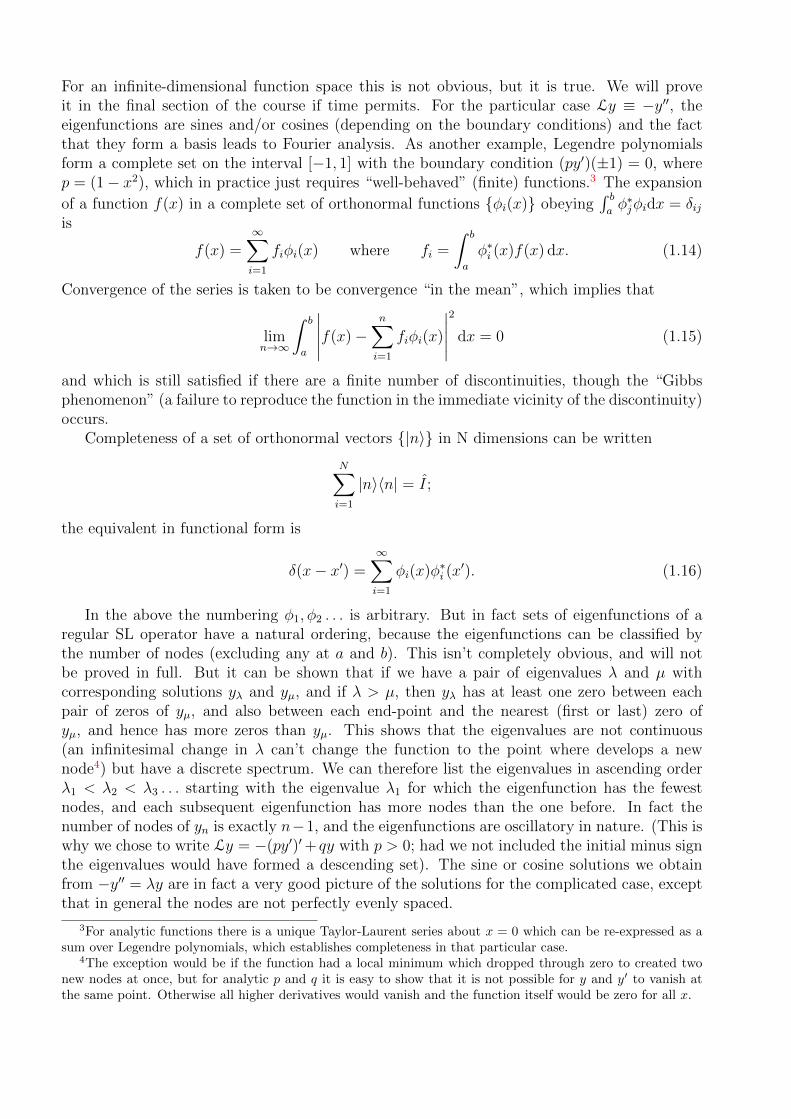
For an infinite-dimensional function space this is not obvious, but it is true. We will proveit in the final section of the course if time permits. For the particular case Ly ≡ −y′′, theeigenfunctions are sines and/or cosines (depending on the boundary conditions) and the factthat they form a basis leads to Fourier analysis. As another example, Legendre polynomialsform a complete set on the interval [−1, 1] with the boundary condition (py′)(±1) = 0, wherep = (1− x2), which in practice just requires “well-behaved” (finite) functions.3 The expansion

of a function f(x) in a complete set of orthonormal functions {φi(x)} obeying∫ baφ∗jφidx = δij

is

f(x) =∞∑i=1

fiφi(x) where fi =

∫ b

a

φ∗i (x)f(x) dx. (1.14)

Convergence of the series is taken to be convergence “in the mean”, which implies that

limn→∞

∫ b

a

∣∣∣∣∣f(x)−n∑i=1

fiφi(x)

∣∣∣∣∣2

dx = 0 (1.15)

and which is still satisfied if there are a finite number of discontinuities, though the “Gibbsphenomenon” (a failure to reproduce the function in the immediate vicinity of the discontinuity)occurs.

Completeness of a set of orthonormal vectors {|n〉} in N dimensions can be written

N∑i=1

|n〉〈n| = I;

the equivalent in functional form is

δ(x− x′) =∞∑i=1

φi(x)φ∗i (x′). (1.16)

In the above the numbering φ1, φ2 . . . is arbitrary. But in fact sets of eigenfunctions of aregular SL operator have a natural ordering, because the eigenfunctions can be classified bythe number of nodes (excluding any at a and b). This isn’t completely obvious, and will notbe proved in full. But it can be shown that if we have a pair of eigenvalues λ and µ withcorresponding solutions yλ and yµ, and if λ > µ, then yλ has at least one zero between eachpair of zeros of yµ, and also between each end-point and the nearest (first or last) zero ofyµ, and hence has more zeros than yµ. This shows that the eigenvalues are not continuous(an infinitesimal change in λ can’t change the function to the point where develops a newnode4) but have a discrete spectrum. We can therefore list the eigenvalues in ascending orderλ1 < λ2 < λ3 . . . starting with the eigenvalue λ1 for which the eigenfunction has the fewestnodes, and each subsequent eigenfunction has more nodes than the one before. In fact thenumber of nodes of yn is exactly n−1, and the eigenfunctions are oscillatory in nature. (This iswhy we chose to write Ly = −(py′)′+ qy with p > 0; had we not included the initial minus signthe eigenvalues would have formed a descending set). The sine or cosine solutions we obtainfrom −y′′ = λy are in fact a very good picture of the solutions for the complicated case, exceptthat in general the nodes are not perfectly evenly spaced.

3For analytic functions there is a unique Taylor-Laurent series about x = 0 which can be re-expressed as asum over Legendre polynomials, which establishes completeness in that particular case.

4The exception would be if the function had a local minimum which dropped through zero to created twonew nodes at once, but for analytic p and q it is easy to show that it is not possible for y and y′ to vanish atthe same point. Otherwise all higher derivatives would vanish and the function itself would be zero for all x.

1.2.3 Application to quantum mechanics and casting equations inSturm-Liouville form

The properties above (real eigenvalues, discrete spectrum with a lowest or “ground state”eigenvalue, oscillatory solutions with an extra node each time we go up a level) are exactlythose that we have frequently met before in quantum-mechanical problems. In one-dimensionthe Schrodinger equation is clearly an example of an SL equation (where p(x) = ~2/2m =constand q(x) = V (x)) and the boundary conditions we impose are always homogeneous to preservethe important principle of superposition. However when we separate the Schrodinger equationin plane or spherical polar coordiates we obtain radial equations which are not SL in form, forinstance in a 2D infinite square well, for solutions with angular dependence einφ, we obtain theradial equation

r2R′′(r) + rR′(r) + (k2r2 − n2)R(r) = 0 with k =√

2mE/~ and R(a) = 0. (1.17)

Comparing with the general form of Eq. (1.8), we have p0 = r2, q0 = −n2 and p1 = r 6= p′0.(Note n2 is just a parameter in the radial equation, related to the angular momentum.) Thisis a (generalised) eigenvalue problem with λ = k2, but it is not of SL form.5 Can we salvageanything?

The answer is yes. Any 2nd-order linear differential operator such as the LHS of Eq. (1.8)can be cast in SL form by multiplying throughout by an integrating factor w(x), chosen so thatwp1 = (wp0)

′. This gives

w′ = w

(p1p0− p′0p0

)⇒ w(x) =

1

p0exp

(∫ x p1(x′)

p0(x′)dx′). (1.18)

In this case p1/p0 = 1/r and w(r) = 1/r, giving a new equation with the same eigenvalues andeigenfunctions as before, but now in manifestly SL form:

−(rR′)′ +n2

rR = k2rR.

The point r = 0 is a regular singular point. The boundary condition is R(a) = 0; becausep(0) = 0 the condition at the origin is just that R(0) is finite.

This transformation lets us see that all the desirable properties of an SL equation still hold.The only thing to note is that there is a weight function ρ = r in the orthogonality relation.Of course, this is exactly what we expect from the physical problem, with the element of areabeing dS = 2πr dr. (The corresponding 3D problem has r2 as the weight function.) If the

nodes of the nth Bessel function are z(n)i , the solutions are Jn(kir), where ki = z

(n)i /a.

Another examples of an equation that occurs in QM is Hermite’s:

y′′(z)− 2zy′(z) + 2ny(z) = 0. (1.19)

Again it is not in SL form, although it arises from the Schrodinger equation with a 1D quadraticpotential. The full wave function is expressed as a polynomial times a function which gives theright long-distance behaviour (e−z

2/2 in suitably-scaled coordinates), and some manipulationyields the Hermite equation for the polynomials. The integrating factor w(z), and hence theweight factor ρ(z), is e−z

2, so the wave functions obey the expected orthogonality conditions.6

5Setting z = kr allows us to write this as Bessel’s equation, with solution R(r) = Jn(kr), which is very usefulexcept that it no longer looks like an eigenvalue equation.

6For the quadratic potential V = 12mω

2x2 the scaling is the usual z = x/x0 with x0 =√

~/mω, andE = (n+ 1

2 )~ω. The boundary conditions require n to be an integer.

In the general case we need to check that the new weight function is finite and positiveon x ∈ (a, b). For reference we give the expansion and completeness properties for a set of

functions obeying generalised orthogonality∫ bay∗jρyidx = 0:

f(x) =∞∑i=1

fiφi(x) where fi =

∫ b

a

ρ(x)φ∗i (x)f(x)dx. (1.20)

and

δ(x− x′) =∞∑i=1

φi(x)φ∗i (x′)ρ(x′). (1.21)

1.3 Generating functions

Arfken 12.1,14.1, 15.1,15.3

Riley 18.1,18.5

1.3.1 Legendre polynomials

Consider the problem in electrostatics of finding the potential at a point r near the origin of acharge placed on the z-axis at r0 = r0ez. We know the answer of course:

Φ(r) ∝ 1

|r− r0|=

1√r2 + r20 − 2rr0 cos θ

(1.22)

However we also know that the electric potential must satisfy the Laplace equation ∇2Φ(r) = 0except at r = r0, and that the general axially-symmetric solution is

Φ(r, θ) =∑l

(Al r

l +Bl

rl+1

)Pl(cos θ) (1.23)

Now it will not be possible to find a single solution of this form valid everywhere: Φ has to befinite both at r = 0 and at r →∞, and only Al = Bl = 0 would allow that. But we are familiarwith the idea that a series expansion may have a restricted radius of convergence. In this case,the expression in Eq. (1.22), for any fixed cos θ, can be expanded as a Taylor series about thethe origin, involving only positive powers of r, but that series will have radius of convergencer0—the distance to the position of the charge.7 For r > r0 we would need a Laurent series, inthis case involving only negative powers of r, instead.

So we have (working in units where r0 = 1 for simplicity)

1√1 + r2 − 2r cos θ

=∞∑l=0

Al rl Pl(cos θ) for |r| < 1

It remains to find the constants Al which we do by considering the expression for cos θ = 1,recalling that with the conventional normalisation Pl(1) = 1. Since (1− r)−1 = 1 + r+ r2 + . . .for |r| < 1, we see that Al = 1 for all l: So we have

1√1 + r2 − 2r cos θ

=∞∑l=0

rl Pl(cos θ) for |r| < 1.

This expression is called the generating function g(cos θ, r) for the Legendre polynomials: Usu-ally the two variable are relabelled, r → t and cos θ → x: then

g(x, t) =1√

1 + t2 − 2xt=∞∑l=0

tl Pl(x) for |t| < 1. (1.24)

By constructing the Taylor series in t for the LHS we can read off expressions for the Pl.

g(x, t) =(1− (2tx− t2))−12 = 1 + 1

2(2tx− t2) + 3

8(2tx− t2)2 + 5

16(2tx− t2)3 + 35

128(2tx− t2)4 + . . .

=1 + 12(2tx− t2) + 3

8(4t2x2 − 4xt3 + t4) + 5

16(8t3x3 − 12t4x2 + . . .) + 35

128(16t4x4 + . . .) + . . .

=1t0 + xt+(32x2 − 1

2

)t2 +

(52x3 − 3

2x)t3 +

(358x4 − 15

4x2 + 3

8

)t4 + . . .

7Mathematically, Eq. (1.22), regarded as a function of complex r at fixed real cos θ, has non-analytic pointsat r = e±iθ; for θ = 0, π these merge to give a simple pole at r = ±1, otherwise there are two branch points.

where in the last two lines we have dropped all terms of order t5 or higher. From this we canread off the first five Legendre polynomials, eg P4(x) =

(358x4 − 15

4x2 + 3

8

).

This provides one way of obtaining the polynomials, but it is more useful for obtaining whatare called recurrence relations which relate polynomials of different orders. If for instance wedifferentiate g(x, t) with respect to t we get

∂g

∂t=

x− t(1− 2tx+ t2)3/2

=x− t

1− 2tx+ t2g(x, t)

⇒∞∑n=0

n tn−1 Pn(x) =x− t

(1− 2tx+ t2)

∞∑n=0

tn Pn(x)

⇒∞∑n=0

(n(tn−1 − 2xtn + tn+1) + (tn+1 − xtn)

)Pn(x) = 0

⇒∞∑n=0

ntn−1 Pn(x)−∞∑n=0

(2n+ 1)tnxPn(x) +∞∑n=0

(n+ 1)tn+1 Pn(x) = 0.

By shifting the summation variable n → n± 1 in the first and last terms, and regrouping, weget

∞∑n=0

((n+ 1)Pn+1(x)− (2n+ 1)xPn(x) + nPn−1(x)

)tn = 0.

By collecting powers of t, we get from t0, P1(x) = xP0(x), which we know to be correct, andfrom tn for n ≥ 1, the three-term recurrence relation

(n+ 1)Pn+1(x)− (2n+ 1)xPn(x) + nPn−1(x) = 0 (1.25)

which we can easily check holds for n = 1, 2, 3 from the forms we deduced above.Differentiating with respect to x gives another type of relation, one involving the derivatives

of the polynomials. By a method similar to the above, we get∞∑n=0

tnP ′n(x) =t

(1− 2tx+ t2)

∞∑n=0

tn Pn(x)

⇒∞∑n=0

(tn − 2tn+1x+ tn+2)P ′n(x)− tn+1 Pn(x) = 0

⇒ P ′n−1(x)− 2xP ′n(x) + P ′n+1(x) = Pn(x) for n > 0,

or combining with the derivative of Eq. (1.25), we also get

P ′n+1(x)− P ′n−1(x) = (2n+ 1)Pn(x) and (1− x2)P ′n(x) = nPn−1(x)− nxPn(x).

Various other related relations can be found; in addition differentiating the second of these andcombining with the first leads in a couple of lines to Legendre’s equation

(1− x2)P ′′n (x)− 2xP ′n(x) + n(n+ 1)Pn(x) = 0 (1.26)

which is a further check on the approach. Some textbook define the Legendre polynomials viathe generating function and derive the equation that they satisfy; we have used the oppositeapproach as more physically motivated. Legendre polynomials arise in many problems wherethe equations have spherical symmetry and the solutions are axially symmetric about the z-axis; further solutions which break the axial symmetry involve associated Legendre polynomials(spherical harmonics). If the boundarys are such that poles (cos θ = ±1) are not in the domain,the second solutions Qn(cos θ) will enter as well; we found Q1(x) above (see Eq. (1.7)) and wewill discuss these further in section 1.4.1.

1.3.2 Bessel functions of integer order

For Bessel functions, (solutions to Eq. (1.17)) we use a similar approach. In the 2-d x-y plane,one solution to the wave equation is the plane wave ei(ky−ωt), with ω/c = k. However separatingfirst in time and space and then in plane polar coordinates gives the general solution to thewave equation, in a region containing the origin, as follows:(

A0J0(kr) +∞∑n=1

(Aneinφ +Bne−inφ

)Jn(kr)

)e−iωt

where the sum is over integer n. Substituting y = r sinφ = r(eiφ− e−iφ)/(2i) in the plane wave,setting eiφ = t and kr = z, and equating the two forms gives

exp(z2

(t− 1

t

))= A0J0(z) +

∞∑n=1

(Antn +Bnt

−n)Jn(z)

Symmetry under t → −1/t means that Bn = (−1)nAn, and the value at t = 0 sets A0 = 1 ifJ0(0) = 1, as is conventional (all the others vanish at the origin). This time, the conventionalnormalisation of all the Bessel functions is defined such that An = 1 for all n, and hence wehave the generating function g(z, t) obeying

g(z, t) = exp(z2

(t− 1

t

))= J0(z) +

∞∑n=1

(tn + (−1)nt−n)Jn(z) =∞∑

n=−∞

tnJn(z) (1.27)

Recall that Bessel’s equation only depends on n2 so we are free to define J−n(z) = (−1)nJn(z),which then allows us to rewrite the sum as in the second form above.

Bessel functions are not terminating polynomials, so all we can obtain directly from Eq. (1.27)is a Taylor series expansion of the solution. For instance taking the Taylor expansion in z ofthe LHS and gathering terms independent of t gives

J0(z) =∞∑

j=0,2...

(−1)j/2zj

((j/2)!)22j=

∞∑m=0,1...

(−1)m

(m!)2

(z2

)2m(1.28)

which is even in z and has vanishing derivative at the origin; this series has an infinite radiusof convergence.

Differentiating wrt z or t gives the useful recurrence relations

Jn−1(z)− Jn+1(z) = 2J ′n(z) and Jn+1(z) + Jn−1(z) =2n

zJn(z).

The first of these gives J1(z) = J ′0(z), which tells us that J1(z) is odd and linear about theorigin. In general the first term in the expansion of Jn is proportional to zn, and is odd (even)for odd (even) n.

As with the Legendre case, these recurrence relations can be manipulated till they take theform of Bessel’s equation. This obvious fact is of more relevance in this case, because in thenext section we will see that Bessel functions of non-integer order are also of interest; this showsthat they also obey the recurrence relations.

1.3.3 Hermite polynomials

Here we state without proof a generating function for Hermite polynomials:

g(x, t) = e−t2+2tx =

∞∑n=0

Hn(x)tn

n!.

1.3.4 Rodrigues’ Formula

Rodrigues’ Formula gives different form of generating function for a restricted class of equationsof the form (see Eq. (1.8))

p0(x)y′′(x) + p1(x)y′(x) = −λy(x) (1.29)

where the pi are polynomial, p0 being at most quadratic and p1, linear in x. In that case theintegrating function w(x) defined in Eq. (1.18) will be calculable. Then it can be shown thatthe nth regular eigenfunction is given by

yn =1

w(x)

(d

dx

)n (w(x)

(p0(x)

)n)So for example for Hermite’s equation (1.19), p0 = 1, p1 = −2x, w = e−x

2and

Hn(x) = ex2( d

dx

)ne−x

2

and for Legendre’s equation (1.26) (with conventional normalisation)

Pn(x) =(−1)n

2nn!

( d

dx

)n(1− x2)n

The general proof of Rodrigues’ formula is given in Arfken 12.1 and (for specific cases) Riley18.1, 18.9, and will not be given here though it is not too complicated.

Such equations (Laguerre’s is another) have terminating polynomial solutions. Bessel’sfunction is not of this form, though it might initially appear so at least for n = 0, as when theweight function x2 is divided out, p0 = 1 and p1 = 1/x.

1.4 Series solutions to differential equations

Arfken 8.3, 14.1, 14.3, 15.6

Riley 16 Series solutions to differential equations were introduced in PHYS20171 Maths ofWaves and Fields. This section is mostly revision, but we comment on the results in the lightof our previous work. In particular we find that we need to use a different method if we areexpanding about a regular singular point, and that other singular points will restrict the radiusof convergence of the series. Note that we start without imposing boundary conditions andhence expect to find two solutions for each equation.

1.4.1 Series solutions about ordinary points

Given a differential equation we can expand the solution about an ordinary point of the equationx = x0 as a Taylor series which will in general have a radius of convergence governed by thedistance to the nearest singular point. For example for the classical equation of SHM,

−y′′(x) = y,

expanding about the origin we write

y(x) =∑n=0

anxn,

-1.0 -0.5 0.5 1.0

-1.0

-0.5

0.5

1.0

-1.0 -0.5 0.5 1.0

-3

-2

-1

1

2

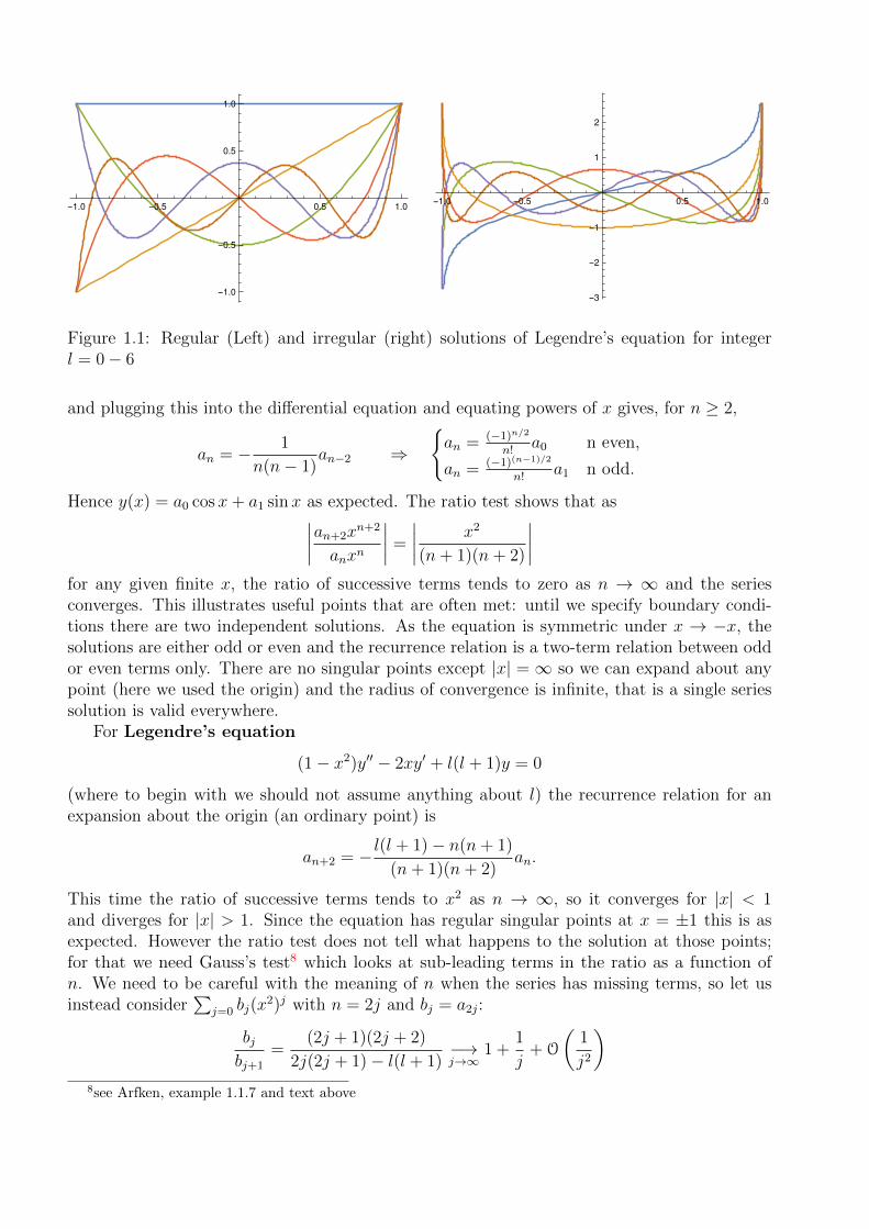
Figure 1.1: Regular (Left) and irregular (right) solutions of Legendre’s equation for integerl = 0− 6

and plugging this into the differential equation and equating powers of x gives, for n ≥ 2,

an = − 1

n(n− 1)an−2 ⇒

{an = (−1)n/2

n!a0 n even,

an = (−1)(n−1)/2

n!a1 n odd.

Hence y(x) = a0 cosx+ a1 sinx as expected. The ratio test shows that as∣∣∣∣an+2xn+2

anxn

∣∣∣∣ =

∣∣∣∣ x2

(n+ 1)(n+ 2)

∣∣∣∣for any given finite x, the ratio of successive terms tends to zero as n → ∞ and the seriesconverges. This illustrates useful points that are often met: until we specify boundary condi-tions there are two independent solutions. As the equation is symmetric under x → −x, thesolutions are either odd or even and the recurrence relation is a two-term relation between oddor even terms only. There are no singular points except |x| =∞ so we can expand about anypoint (here we used the origin) and the radius of convergence is infinite, that is a single seriessolution is valid everywhere.

For Legendre’s equation

(1− x2)y′′ − 2xy′ + l(l + 1)y = 0

(where to begin with we should not assume anything about l) the recurrence relation for anexpansion about the origin (an ordinary point) is

an+2 = − l(l + 1)− n(n+ 1)

(n+ 1)(n+ 2)an.

This time the ratio of successive terms tends to x2 as n → ∞, so it converges for |x| < 1and diverges for |x| > 1. Since the equation has regular singular points at x = ±1 this is asexpected. However the ratio test does not tell what happens to the solution at those points;for that we need Gauss’s test8 which looks at sub-leading terms in the ratio as a function ofn. We need to be careful with the meaning of n when the series has missing terms, so let usinstead consider

∑j=0 bj(x

2)j with n = 2j and bj = a2j:

bjbj+1

=(2j + 1)(2j + 2)

2j(2j + 1)− l(l + 1)−→j→∞

1 +1

j+ O

(1

j2

)8see Arfken, example 1.1.7 and text above

Since the coefficient of 1/j, 1, is not greater than 1, the series diverges. (We get the same resultif we let n = 2j + 1 for the odd series.)

We know the way out: for integer even or odd l the even or odd series will have al+2 = 0 andthe series terminates. The resulting finite polynomial Pl(x) converges for all finite x.) The otherseries, Ql(x), does not terminate and only converges for |x| < 1; boundary conditions requiringwell-behaved solutions at x = ±1 then excludes this second solution. In a familiar pattern,therefore, requiring solutions with certain boundary conditions quantises the eigenvalues—inthis case, this corresponds to the quantisation of orbital angular momentum.

Of course we saw near the start that we could also construct a second solution given onesolution. We constructed Q1(x) (Eq. (1.7)), which can be shown to have the Taylor expansion

Q1(x) = −1 +∑

n=2,4...

xn

(n− 1)

in accordance with the recurrence relation.On a domain x ∈ [a, b] with |a|, |b| < 1, with separable homogeneous boundary conditions,

Legendre’s equation is a regular SL problem with eigenvalue λ which it is not particularly usefulto write as l(l+ 1). We know therefore that the spectrum will be non-degenerate (the solutionswill can be written as superpositions of Pl and Q− L for non-integer l), there will be a lowesteigenvalue corresponding to a solution with no nodes, and higher eigenvalues correspond tomore and more nodes, without bound. If |a| or |b| = 1 the problem is no longer regular (p(±1)is not finite and ±1 are regular singular points) but the same properties persist.

Hermite’s equation presents nothing fundamentally new; the origin is an ordinary pointand the series solution converges for all finite x; however the function grows as ex

2/2 for x→∞,a problem which is solved if the eigenparameter n is an even or odd integer, in which case theeven or odd series terminates.

1.4.2 Frobenius’s method and Bessel functions

Bessel’s equation9

x2y′′ + xy′ + (x2 − n2)y = 0

is more interesting, because the origin is a regular singular point and one might expect problems.Note we write the parameter as n2 and will not necessarily assume integer n, but we will takeit non-negative. If n is known to be non-integer, we write it as ν.

For this case we will use the more general form of a series solution due to Frobenius, andwrite

y(x) = xs∑j=0

ajxj

where s is the lowest power of x in the expansion and its coefficient a0 is by definition non zero.(Note a0 is no longer necessarily the coefficient of x0, which can cause confusion.) This allowsfor a pole or branch point at x = 0 if s < 0, but also for a solution that starts with x or a

9It should be noted that while Bessel’s equation looks like an eigenvalue equation with λ = −ν2, this is nothow it arises in physics; rather ν is an externally-imposed parameter related to the single-valued, finite angularpart of the solution (for instance in 2D ν = m, an integer, or, as we will see, in 3D ν = l+ 1

2 , hence half integer).Rather, the variable x arises as kr, with k related to the energy (QM) or frequency (classical vibrations). Thenk2 is the eigenvalue, and a homogeneous boundary condition at a finite r = R result in discretisation of k.

2 4 6 8 10

-0.4

-0.2

0.2

0.4

0.6

0.8

1.0

2 4 6 8 10

-2.0

-1.5

-1.0

-0.5

0.5

1.0

Figure 1.2: Regular (left) and irregular (right) solutions of Bessel’s equation for integer n = 0−5

higher power of x. the equation becomes∑j=0

((j + s)(j + s− 1) + (j + s)− n2

)ajx

j+s +∑j=0

ajxj+s+2 = 0

⇒ (s2 − n2)a0xs + ((s+ 1)2 − n2)a1x

s+1 +∑j=2

(((j + s)2 − n2

)aj + aj−2

)xj+s = 0

The recurrence relation is

aj =1

n2 − (j + s)2aj−2 for j ≥ 2

but in addition we need the first two terms to vanish. The first gives

s2 − n2 = 0

which is called the indicial equation, and requires s = ±n. (Recall that a0 6= 0 by definition: xs

is the lowest power in the series.) If s = −12, a1 6= 0 is allowed though not required, otherwise

we need a1 = 0. For s = −12, the series built on a1 will start with x

12 . However if s = −1

2is

one possibility, so is s = 12

and this already gives a series starting at x12 ; we don’t get anything

new. So either way we can set a1 to zero, and obtain our two solutions (if they exist) from thetwo values of s. Unless s = n = 0, one of these by definition will be ill-defined at the origin,the other will start with the power xn—as indeed we already found to be true for integer n.

Starting with the case n = 0, s = 0 and we just have aj = − 1j2aj−2. Setting a0 = 1,

J0(x) =∑

j=0,2...

(−1)j/2

(j!!)2xj

where j!! = j(j − 2)(j − 4) . . . = 2j/2(j/2)! for even j. This is the same as we found before, seeEq. (1.28). But there is no other series solution!

For other integer n > 0, if we take s = n the solution will be of the form xnf(x2) which willbe odd or even as n is odd or even, and with aj = −aj−2/j(j + 2n) for j ≥ 2,

Jn(x) =∑

m=0,1...

(−1)m

m!(m+ n)!

(x2

)n+2m

where the normalisation matches that obtained from the generating function. Now if we takes = −n we might expect to get a second solution, albeit one that is not regular at the origin,but the recurrence relation is aj = −aj−2/j(j − 2n) which fails when j = 2n. So again we donot get a second series solution.

Of course a second solution must exist, and is denoted Yn(x) or Nn(x), but its behaviour atthe origin must not be describable by a power series, even one with negative powers. log x issuch a function (though not one of the solutions itself).

Note that we assumed positive n and found a solution for s = n; if we assume negative nwe have a solution for (positive) s = −n. As the equation only depends on n2 the two casesare not independent. Recall above we chose to define J−n(z) = (−1)nJn(z) for integer n.

Moving on to non-integer n = ν, with ν > 0, we can in fact reuse much of the analysisabove. We have to define Γ(α) which has the value (α − 1)! for integer α > 0, and whichsatisfies

Γ(α) = (α− 1)(α− 2)(α− 3) . . . (α−N)Γ(α−N)

For s = ν, and using conventional normalisation in the second step,

Jν(x) = Aνxν∑

m=0,1...

(−1)mΓ(ν + 1)

22mm!Γ(m+ ν + 1)x2m =

∑m=0,1...

(−1)m

m!Γ(m+ ν + 1)

(x2

)ν+2m

.

Replacing ν → −ν gives J−ν which is an independent solution, albeit one which is not regularat the origin.

All of the series given above clearly converge for all x > 0.For non-integer ν it is actually conventional to define the second solution via

Nν =cos(νπ)Jν − J−ν

sin(νπ)

which clearly forms a linearly-independent pair with Jν since it contains J−ν . For integer ν = nboth the numerator and denominator vanish (recall J−n = (−1)nJn) but the expression canbe evaluated using l’Hopital’s rule (in ν) and used to define Nn as well. As expected it is(logarithmically) divergent at the origin.

Finally for n = ν = 12, we note that for integer m,

m!Γ(m+ 1 + 12) = m!Γ(1

2)12· 32· 52. . . 2m+1

2

= (2m)!!(2m+ 1)!!2−(2m+1)Γ(12) = (2m+ 1)!2−(2m+1)Γ(1

2)

so

J 12(x) =

212

Γ(12)x

12

∑m=0,1...

(−1)m

(2m+ 1)!x2m+1 ∝ sinx√

x.

and J− 12(x) ∝ cosx/

√x.

Bessel functions of half-integer order turn out to be useful for the solution of the waveequation in spherical polar coordinates. The radial wave function satisfies

r2R′′(r) + 2rR′(r) + (k2r2 − l(l + 1))R(r) = 0,

and with the substitution R(r) = u(r)/r, for l = 0, we obtain u(r) = A cos(kr) + B sin(kr).However the alternative substitution R(r) = u(kr)/

√kr transforms the equation into Bessel’s

equation with ν = l + 12. For l = 0 that gives the same as the simpler substitution, but we

also now have a way of finding solutions for higher l. These occur enough that they are calledspherical Bessel functions and given special symbols:

jl(x) =

√π

2xJl+

12(x), nl(x) =

√π

2xJ−l−1

2(x).

A final comment on Frobenius’s method: if we use if when we don’t need to, that is for anexpansion about an ordinary point, we will find that the indicial equation has solutions s = 0and s = 1. If, further, the equation has symmetry under x → −x, such that we expect oddor even solutions, the solution we obtain for s = 1 will be the same as the one built on a1 fors = 0.

1.5 Recap of common differential equations in Physics

A number of these equations, particularly those based on the Laplacian, are scale invariant sothey have the same form under x→ x0z.

Where the equations, such as those based on the wave equation or free Schrodinger equation,are not scale invariant, the scale k is usually treated as an eigenvalue that allows us to satisfyseparated boundary condition, giving rise to discrete vibrational modes or energy levels. Whereappropriate the scaled and unscaled forms are both given.

Many of the equations below arise from PDEs after separation of variables. In particularwhat we are calling “the wave equation” (or Schrodinger equation) is actually the equation forthe spatial part. The full solution takes the form f(r)e−iωt, where f(r) satisfies

∇2f(r) + k2f(r) = 0, (1.30)

and k2 is related to ω by the dispersion relation. Then in 2D we write f(r) = R(r)eimφ

and R(r) satisfies Bessel’s equation of order m; in 3D we write f(r) = R(r)Pml (cos θ)eimφ ∝

R(r)Y ml (θ, φ) where Pm

l (z) satisfies the associated Legendre equation, and R(r) satisfies anequation related to Bessel’s equation of order (l + 1

2). The parameters m and l are related

to the separation constants; they are eigenvalues fixed by the boundary conditions (eg single-valued, finite solutions) in the angular equations but simply parameters in the radial equations.(In QM of course they are related to the angular momentum; in classical applications theyare related to the multipole moments of the solution.) Thus not every parameter in “q(x)” istreated as an eigenvalue in the conventional applications of these equations.

For k2 = 0 we just have the Laplace equation; the angular equations are exactly as abovebut the radial equations are simpler and have solutions which are just powers of r.

The wave equations all have version with an eigenvalue of the opposite sign, k2 → −κ2, thisarises in the diffusion equation. In 1D the solutions are decaying and growing exponentials. In2D they are termed modified (spherical) Bessel functions In(κr) and Kn(κr) and also decay orgrow exponentially at large values of r; there are spherical analogues with similar propertiesfor the 3D problem.

Below, where the second solution is rarely encountered and has no standard name, it issimply represented by dots.

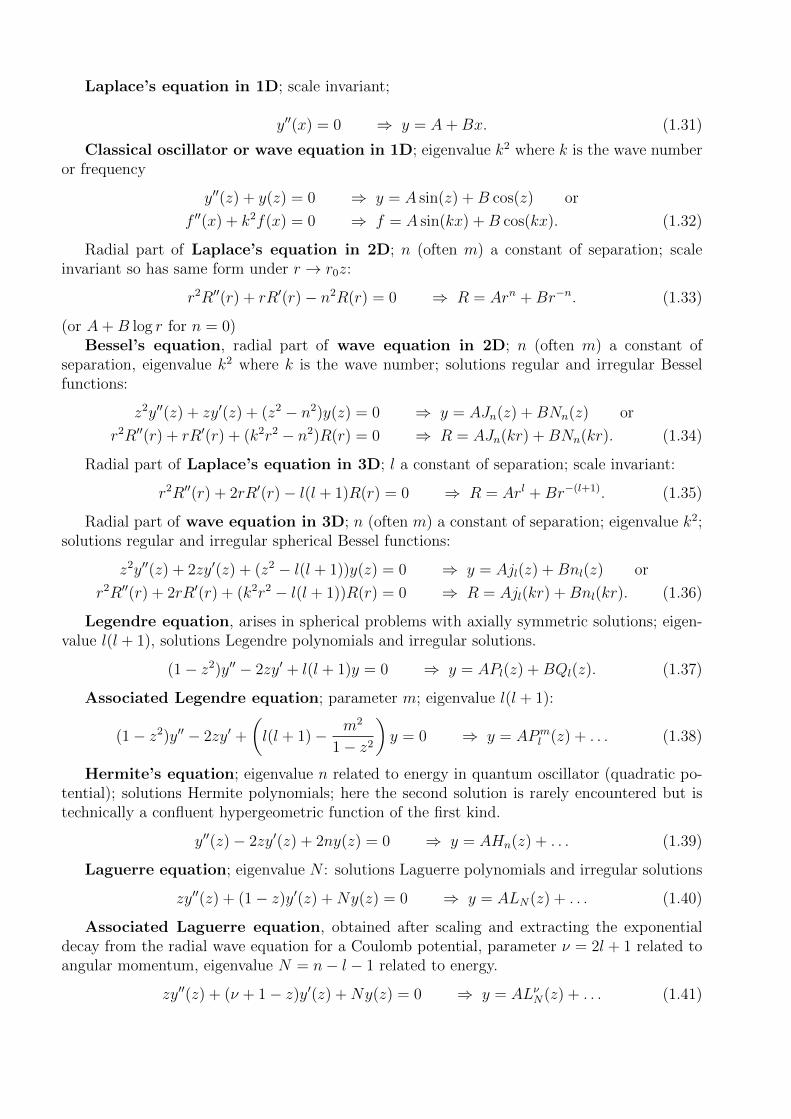
Laplace’s equation in 1D; scale invariant;

y′′(x) = 0 ⇒ y = A+Bx. (1.31)

Classical oscillator or wave equation in 1D; eigenvalue k2 where k is the wave numberor frequency

y′′(z) + y(z) = 0 ⇒ y = A sin(z) +B cos(z) or

f ′′(x) + k2f(x) = 0 ⇒ f = A sin(kx) +B cos(kx). (1.32)

Radial part of Laplace’s equation in 2D; n (often m) a constant of separation; scaleinvariant so has same form under r → r0z:

r2R′′(r) + rR′(r)− n2R(r) = 0 ⇒ R = Arn +Br−n. (1.33)

(or A+B log r for n = 0)Bessel’s equation, radial part of wave equation in 2D; n (often m) a constant of

separation, eigenvalue k2 where k is the wave number; solutions regular and irregular Besselfunctions:

z2y′′(z) + zy′(z) + (z2 − n2)y(z) = 0 ⇒ y = AJn(z) +BNn(z) or

r2R′′(r) + rR′(r) + (k2r2 − n2)R(r) = 0 ⇒ R = AJn(kr) +BNn(kr). (1.34)

Radial part of Laplace’s equation in 3D; l a constant of separation; scale invariant:

r2R′′(r) + 2rR′(r)− l(l + 1)R(r) = 0 ⇒ R = Arl +Br−(l+1). (1.35)

Radial part of wave equation in 3D; n (often m) a constant of separation; eigenvalue k2;solutions regular and irregular spherical Bessel functions:

z2y′′(z) + 2zy′(z) + (z2 − l(l + 1))y(z) = 0 ⇒ y = Ajl(z) +Bnl(z) or

r2R′′(r) + 2rR′(r) + (k2r2 − l(l + 1))R(r) = 0 ⇒ R = Ajl(kr) +Bnl(kr). (1.36)

Legendre equation, arises in spherical problems with axially symmetric solutions; eigen-value l(l + 1), solutions Legendre polynomials and irregular solutions.

(1− z2)y′′ − 2zy′ + l(l + 1)y = 0 ⇒ y = APl(z) +BQl(z). (1.37)

Associated Legendre equation; parameter m; eigenvalue l(l + 1):

(1− z2)y′′ − 2zy′ +

(l(l + 1)− m2

1− z2

)y = 0 ⇒ y = APm

l (z) + . . . (1.38)

Hermite’s equation; eigenvalue n related to energy in quantum oscillator (quadratic po-tential); solutions Hermite polynomials; here the second solution is rarely encountered but istechnically a confluent hypergeometric function of the first kind.

y′′(z)− 2zy′(z) + 2ny(z) = 0 ⇒ y = AHn(z) + . . . (1.39)

Laguerre equation; eigenvalue N : solutions Laguerre polynomials and irregular solutions

zy′′(z) + (1− z)y′(z) +Ny(z) = 0 ⇒ y = ALN(z) + . . . (1.40)

Associated Laguerre equation, obtained after scaling and extracting the exponentialdecay from the radial wave equation for a Coulomb potential, parameter ν = 2l + 1 related toangular momentum, eigenvalue N = n− l − 1 related to energy.

zy′′(z) + (ν + 1− z)y′(z) +Ny(z) = 0 ⇒ y = ALνN(z) + . . . (1.41)

1.6 Transform methods

1.6.1 Fourier Transforms: differential equations defined on an infi-nite interval

Arfken 20.2-4

Riley 13.1

Frequently met boundary conditions are that the solution to a differential equation be squareintegrable, vanishing at x = ±infty. Assuming suitable conditions on its continuity, such asolution y(x) will have a Fourier Transform y(k) defined as

y(k) =

∫ ∞−∞

e−ikxy(x)dx, (1.42)

with the inverse being given by

y(x) =1

2π

∫ ∞−∞

eikxy(k)dk, (1.43)

Contrary to usage in, for instance, QM, it proves more useful to distribute the factor of 2πasymmetrically in this course.

Now the Fourier transform of the derivative of y(x) has a simple form:

F.T.[y′] =

∫ ∞−∞

e−ikxdy

dxdx = −

∫ ∞−∞

(d

dxe−ikx

)y(x)dx = iky(k) (1.44)

and similarly the FT of the second derivative is −k2y(k). Thus a differential equation with(positive) constant coefficients can be turned into an algebraic equation for y(k). So

y′′ + 2ay′ + by = f(x) ⇒ y(k) =f(k)

b+ 2ika− k2(1.45)

The issue of course is to find the inverse transform:

y(x) =1

2π

∫ ∞−∞

eikxf(k)

b+ 2ika− k2dk (1.46)

There will be particular functions f(k) for which we can actually do the integral. More gen-erally though, we recall the convolution theorem, that the FT or inverse FT of a product is aconvolution. The IFT of f(k) is of course f(x); let us define the other IFT as

G(x) =1

2π

∫ ∞−∞

eikx1

b+ 2ika− k2dk (1.47)

so

y(x) =

∫ ∞−∞

G(x− z)f(z) dz. (1.48)

The calculation of G(x) may be often done using methods from complex variables, byconsidering an integral in the complex k plane over a semi-circular contour of radius R, suchthat the desired integral is the limit as R → ∞ of the straight section. We invoke Jordan’slemma to say that if x > 0, the contribution from a semicircle in the upper half plane will tend

to 0 as R → ∞. Thus the desired real integral can be equated to the full contour integral,which is evaluated from the residues of the enclosed poles. For x < 0 the contour must insteadbe closed in the lower half plane. Here the poles are at ia±

√b− a2 and assuming b > a2 these

are both in the upper half plane; the result is

G(x) = Θ(x)e−axsin(√

b− a2x)

√b− a2

(1.49)

Recall Θ(x− x0) is a unit step function at x0 and its inclusion here ensures that G(x) vanishesfor x < 0. This is continuous and falls of exponentially as x → ∞, so any reasonable drivingterm f(x) will give a well defined solution, which we can rewrite as

y(x) =

∫ x

−∞G(x− z)f(z) dz. (1.50)

Even if the integral cannot be done analytically, it can be done numerically. This is a generalmethod of finding the particular integral. The complementary function is absent, because inthis case it contains e−ax and so is not finite at x→ −∞.

While we have used x as the variable here, the interpretation is simpler if we think of time; inparticular if we replace a→ γ/2 and b→ ω2

0, we see the problem is the classical underdampedharmonic oscillator with a driving term.

We will meet solutions of this kind much more extensively in the next section.

1.6.2 Laplace Transforms: differential equations with initial condi-tions

Arfken 20.7-10

Riley 13.2, 25.5

Though we are less concerned with these in this course, problems in the time domain arealmost always specified by initial conditions rather than boundary conditions, that is we do notusually specify conditions on a solution at some future time t. Rather we set it up and wantto see how it evolves.

For such problems the Laplace transform is more useful than the Fourier Transform:

F (s) =

∫ ∞0

e−stf(t) dt. (1.51)

Unlike with the F.T. it is hard to assign a physical meaning to the conjugate variable s (some-times called p or other names).

Convergence of the integral may require restrictions on s; for instance if f(t) = eat, F (s) =1/(s− a) only for s > a.

The Laplace transform is insensitive to f(t) for t < 0. It will be unchanged if we replacef(t) by Θ(t)f(t).

In practice the inverse is normally found via look-up tables such as Table 1.1. If F (s) is theL.T. of f(t), then Θ(t)f(t) is the inverse Laplace transform of F (s). The Θ(t) is important!

The shift theorems are particularly useful:

F (s− s0)→ es0tf(t)Θ(t) and e−st0F (s)→ f(t− t0)Θ(t− t0) (1.52)

For Laplace transforms, the convolution h(t) of two functions f(t) and g(t) is given by

h(t) = (f ∗ g)(t) =

∫ t

0

f(u)g(t− u) du. (1.53)

This agrees with the previous definition (with an integral from −∞ → ∞) if both functionsvanish for negative values of their argument. The inverse Laplace transform of a productH(s) = F (s)G(s) is the convolution h(t) = f ∗ g.

The inverse Laplace transform may be computed using the Bromwich integral, in which sis treated as a complex variable lying on a line parallel to the imaginary axis:

f(t) =1

2πi

∫ λ+i∞

λ−i∞estF (s) ds. (1.54)

The offset λ must be positive, and large enough so that the line of integration lies to the rightof all poles of F (s). (For proof, see Arfken 20.10 or Riley 25.5)

λ

If F (s) has only poles, and no more complicated analytic structure such as branch points,we can close the contour of integration as shown in the diagram (green arc). Provided F (s)tends to zero as |s| → ∞, if t > 0 Jordan’s Lemma ensures that contribution of the arc vanishesas the radius is taken to infinity. If t < 0, we close the contour to the right instead. Hence f(t)is just given by Θ(t) times the sum of the residues of estF (s). If F (s) has a branch cut thecontour will be more complicated.

The expressions for the Laplace transforms of the derivatives of f(t),

f ′(t)→ sF (s)− f(0) and f ′′(t)→ s2F (s)− sf(0)− f ′(0). (1.55)

allow us to recast differential equations for f(t) as algebraic ones for F (s). An importantfeature is that the initial conditions on f(t) are incorporated directly. Higher derivatives canalso be included. As before the challenge is to invert F (s); as before the general solution canbe cast as a convolution, but for specific cases it may also be possible to use the look-up tableor the Bromwich integral to do the inversion directly. As a fairly trivial example to illustratethe problem, consider

df

dt+ f(t) = Θ(t)(1−Θ(t− 2)), f(0) = 1 (1.56)

that is a unit driving term which lasts for 2 time units—and could also be written Θ(t)Θ(2− t).

f(t) F (s) =∫∞0e−stf(t)dt Restrictions

11

ss > 0

eat1

s− as > a

tnn!

sn+1s > 0, n a positive integer

t−1/2√π

ss > 0

sin(at)a

s2 + a2s > 0

cos(at)s

s2 + a2s > 0

sinh(at)a

s2 − a2s > a

cosh(at)s

s2 − a2s > a

tnf(t) (−1)ndn

dsn(F (s)) s > 0, n a positive integer

f(t)t

∫∞sF (y)dy s > 0

f(at)1

a

(F (

s

a))

s > 0

f ′(t) sF (s)− f(0) s > 0

f ′′(t) s2F (s)− sf(0)− f ′(0) s > 0

Θ(t− t0)e−st0

st0, s > 0

Θ(t− t0)f(t− t0) e−st0F (s) t0, s > 0

es0tf(t) F (s− s0) s > s0

δ(t− t0) e−st0 t0, s > 0

Table 1.1: Table of common Laplace transforms and useful relations

This gives

sF (s)− 1 + F (s) =

∫ 2

0

e−stdt =1

s(1− e−2s)

⇒ F (s) =1

s− e−2s

s+

e−2s

s+ 1

⇒ f(t) = Θ(t)(

1−Θ(t− 2) + Θ(t− 2) e−(t−2))

= Θ(t)Θ(2− t) + e2Θ(t− 2) e−t.

(1.57)

To reach the second line we used partial fractions to separate 1/s(s+ 1) and for the third linewe used the lookup table including the shift theorem (1.52). The solution is a constant untilthe driving term ceases, then it decays with the natural decay time of the undriven solutione−t.

Coupled differential equations can also be handled with Laplace methods, since one obtainssimultaneous algebraic equations for the corresponding transforms. Laplace methods havebeen extensively used to analyse the propagation of signals though electrical circuits, with theconvolution method allowing for efficient calculation of numerical solutions for a variety ofinputs.