Numerical approximations of Sturm–Liouville … using Chebyshev polynomial expansions method Uğur...

Yücel, Cogent Mathematics (2015), 2: 1045223http://dx.doi.org/10.1080/23311835.2015.1045223

APPLIED & INTERDISCIPLINARY MATHEMATICS | RESEARCH ARTICLE

Numerical approximations of Sturm–Liouville eigenvalues using Chebyshev polynomial expansions methodUğur Yücel1*

Abstract: In this paper, an efficient technique based on the Chebyshev polynomial expansions for computing the eigenvalues of second- and fourth-order Sturm–Liouville boundary value problems is proposed. This technique reduces the given Sturm–Liouville problem to an integral equation. The resulting integral equation is then transformed into the eigenvalue equation by calculating the integrals at the grid points using the Chebyshev expansions. Thus, the required eigenvalues of the given problem are obtained by solving this eigenvalue equation. The excellent performance of this scheme is illustrated through some numerical examples, and comparison with other methods is presented.

Subjects: Applied Mathematics; Mathematics & Statistics; Science

Keywords: Boundary value problems; Chebyshev expansions; eigenvalues; Schrödinger equation; Sturm–Liouville problems

1. IntroductionSturm–Liouville problems (SLPs) arise throughout engineering mathematics. They arise directly as eigenvalue problems in one space dimension. For example, they describe the vibrational modes of various systems, such as the vibrations of a string or the energy eigenfunctions of a quantum mechanical oscillator, in which case the eigenvalues correspond to the resonant frequencies of vibration or energy levels. They also commonly arise from linear PDEs in several space dimensions when the equations are separable in some coordinate system, such as cylindrical or spherical coordinates.

Mathematicians have studied SLPs for over 200 years. It has a highly developed theory and remains an active area of interest. Therefore, in this work, we consider numerical solutions of both second- and fourth-order SLPs described below.

*Corresponding author: Uğur Yücel, Faculty of Arts and Sciences, Department of Mathematics, Pamukkale University, Denizli 20070, TurkeyE-mail: [email protected]

Reviewing editor:Kok Lay Teo, Curtin University, Australıa

Additional information is available at the end of the article

ABOUT THE AUTHORUğur Yücel is a professor in the Department of Mathematics at Pamukkale University, Denizli, Turkey. He received his PhD degree in Applied Mathematics from Lehigh University, Bethlehem, PA, USA. His research interests are focused on labyrinth seals in turbomachinery and numerical solutions of ordinary and partial differential equations.

PUBLIC INTEREST STATEMENT“Sturm–Liouville problems” are famous boundary value problems that naturally arise when solving certain partial differential equation problems using a “separation of variables” method. Mathematicians have studied these problems for over 200 years. They have a highly developed theory and remain an active area of interest. In this work, a numerical approach is developed to obtain approximate eigenvalues of these problems.

Received: 16 December 2014Accepted: 22 April 2015Published: 22 May 2015

© 2015 The Author(s). This open access article is distributed under a Creative Commons Attribution (CC-BY) 4.0 license.

of 13

Uğur Yücel

http://crossmark.crossref.org/dialog/?doi=10.1080/23311835.2015.1045223&domain=pdf&date_stamp=2015-05-22

mailto:[email protected]

http://creativecommons.org/licenses/by/4.0/

of 13


A regular second-order SLP is a second-order linear, homogeneous, ordinary differential equation of the form

together with the seperated (each with one boundary point) homogeneous boundary conditions

where αi and βi, i = 1, 2, are the real constants. In Equation 1, λ is the unknown eigenvalue pertinent to the differential operator defined by the left-hand side of Equation 1, the interval (a, b) is finite, the functions p, p′, q, and w are in L1 (a, b) with p(x) > 0 and w(x) > 0 for x ∈ (a, b). This is distinguished from the case when p or w vanishes at some point in the interval [a, b] or when the interval is of infinite length, in which case the problem is called a singular SLP. For a regular second-order SLP, it is found that all eigenvalues are real and non-negative. In addition, there are infinitely many eigenvalues that are discretely distributed and hence do not fill out any interval. More information on the mathematical theory of second-order SLPs may be found in Amrein, Hinz, and Pearson (2005) and Pryce (1993).

A non-singular fourth-order SLP consists of a fourth-order linear ODE of the form

together with seperated, self-adjoint boundary conditions specified at both ends of the domain (a, b), two boundary conditions at the end x = a, and another two boundary conditions at the end x = b. Basically, there are three types of boundary conditions and their combinations commonly used with Equation 3 in applications. These boundary conditions are given as y = 0, y� = 0 for clamped end, y = 0, y�� = 0 for hinged (or simply supported) end, and y�� = 0, y�� = 0 for free end. The technical conditions for the problem to be non-singular are: the interval (a, b) is finite; the functions P(x), S(x), Q(x), W(x), and 1∕P(x) are in L1 (a, b); and the essential infima of P(x) and W(x) are both positive. Under these assumptions, it is well known that the eigenvalues are bounded from below. They can be ordered as �

0≤ �

1≤ �

2≤ ⋯ ≤ �k ≤ ⋯, where λk → ∞ as k → ∞, and where each eigenvalue has

multiplicity at most 2. More information on the mathematical theory of fourth-order SLPs may be found in Greenberg (1991) and Greenberg and Marletta (1995).

In most cases, it is not possible to obtain the eigenvalues of the above problems analytically. However, there are various approximate methods as, for example, the weighted residual methods, the variational methods, and finite difference and finite elements methods. Extensive literature reviews for the numerical approximations of second-order and fourth-order SLPs can be found in Yücel (2006) and Yücel and Boubaker (2012), respectively. In order to obtain more efficient numerical results, several ways have been devised in the last years. Recently, El-gamel and Abd El-hady (2013) discussed and compared two useful schemes for second-order Sturm–Liouville eigenvalue problems: differential quadrature method (DQM) and collocation method with sinc functions. Saleh Taher, Malek, and Momeni-Masuleh (2013) proposed a new technique based on Chebyshev differentiation matrix for computing eigenvalues of a general class of regular fourth-order SLPs. Yuan, Ye, Xiao, Kennedy, and Williams (2014) introduced the exact dynamic stiffness vibration method for solving regular sec-ond- and fourth-order SLPs. Most recently, Amodio and Settanni (2015) discussed the solution of regu-lar and singular SLPs by means of high-order finite difference schemes. They described a method to define a discrete problem and its numerical solution by means of linear algebra techniques.

In the literature, to the best of the author’s knowledge, there is no study on the Chebyshev poly-nomial expansions (El-gendi’s method) (El-gendi, 1969) applied for SLPs. On the other hand, this method is an efficient discretization technique for obtaining accurate numerical solutions of

(1)−

(p(x) y�

)�+ q(x) y = 𝜆w(x) y , a < x < b,

(2)

�1y(a) + �

2y�(a) = 0, �

2

1+ �

2

2≠ 0

�1y(b) + �

2y�(b) = 0, �

2

1+ �

2

2≠ 0

(3)(P(x)y��

)��−

(S(x) y�

)�+ Q(x) y = 𝜆W(x)y, a < x < b

of 13


differential, integral, and integro-differential equations. El-gendi’s method is based on expanding the unknown function in terms of Chebyshev polynomials. Based on the discrete ortogonality rela-tionships of these polynomials, several methods for solving linear and non-linear ODEs (Fox, 1962) and integral differential equations (Elliott, 1963) were proposed at about the same time. They were found to have considerable advantage over the finite difference methods. Since then, these meth-ods have become standard. They are now part of the larger family of spectral methods (Boyd, 2000). They consist in expanding the unknown function in a series of Chebyshev polynomials, trancating this series, and then substituting the approximation in the actual equation, and finally determining equations for the coefficients. However, El-gendi (1969) described a new method for the numerical solution of differential, integral, and integro-differential equations by computing directly the values of the functions rather than the Chebyshev coefficients. These two approaches are equivalent in the sense that if the function values at some grid points are known, the Chebyshev coefficents for the function can be directly computed. The method has been extended to solve initial value problems in time-dependent quantum field theory and second-order boundary value problems in fluid (Mihaila & Mihaila, 2002). Recently, it has been applied to solve the generalized Kuramoto–Sivashinsky equa-tion (Khater & Temsah, 2008) and convection–diffusion equation (Temsah, 2009).

Our goal in this paper is to extend Chebyshev polynomial expansions, known as El-gendi’s method (El-gendi, 1969), to deal with the second- and fourth-order SLPs given above. To achieve this goal, we first consider the numerical approximations of second-order SLP (1) with Drichlet boundary conditions

Then, we consider numerical approximations of a simple form of Equation 3 with some specified end conditions to demonstrate directly the use of El-gendi’s method on the fourth-order problems. In addition, we choose the fourth-order problems (3) to be squares of the second-order problems (1) for numerical illustrations. This is because if we have a second-order problem with Drichlet boundary conditions given above and the differential operator,

then the corresponding fourth-order problem (3) has the differential operator

where

The boundary conditions, in this case, are

The eigenvalues of the fourth-order problem are then simply the squares of the eigenvalues of the second-order problem which means that they are all non-negative (Greenberg & Marletta, 1995).

This paper is organized as follows. In Section 2, we first review the Chebyshev polynomial expan-sions method (El-gendy’s method), then we give some new formulas for the matrix approximation of integrals which are necessary to deal with higher order problems. The method is then applied to second-order and a simple form of the fourth-order SLPs in Section 3. Numerical examples are dis-cussed in Section 4, and some conclusions are drawn in Section 5.

(4)y(a) = 0, y(b) = 0

(5)�y = −

(p(x)y�

)�+ q(x)y

(6)�2y =

(P(x)y��

)��−

(S(x)y�

)�+ Q(x)y

(7)P = p2, S = 2pq − pp��, Q = q2 − pq�� − p�q�

(8)y(a) = 0, p�(a)y�(a) + p(a)y��(a) = 0

y(b) = 0, p�(b)y�(b) + p(b)y��(b) = 0

of 13


2. The method of Chebyshev polynomial expansionsIn this section, we describe the method of Chebyshev expansion by following closely the procedures outlined in El-gendi (1969). It is assumed that a function y(x), which is continuous and of bounded variation in the interval [-1, 1], can be approximated by

where the summation symbol with double prime indicates that the terms with suffixes i = 0 and i = N are to be halved, Ti(x) is the Chebyshev polynomials of the first kind of degree i ≤ N, and the coeffi-cients ai are defined by

In the equation above, the grid points xj, the so-called Chebyshev points, are given by

The approximate formulae (Equation 9) is exact at x = xj given by Equation 11.

It is known by the Chebyshev trancation theorem (Boyd, 2000) that the error in approximating y(x) by the sum of its first N terms is bounded by the sum of the absolute values of all the neglected coef-ficients. A detailed discussion of this theorem and the convergence theory for Chebyshev polynomi-als can be found in Boyd (2000).

Using the above approximation for the aforementioned function y(x), the integral

at the grid points

can be approximated as

We can now write this equation in matrix form as

where D is a square matrix of order N + 1 and the actual values of the elements of this matrix (dij , i = 0, 1,… ,N, j = 0, 1,… ,N

) can be easily calculated using the right-hand side of Equation 14.

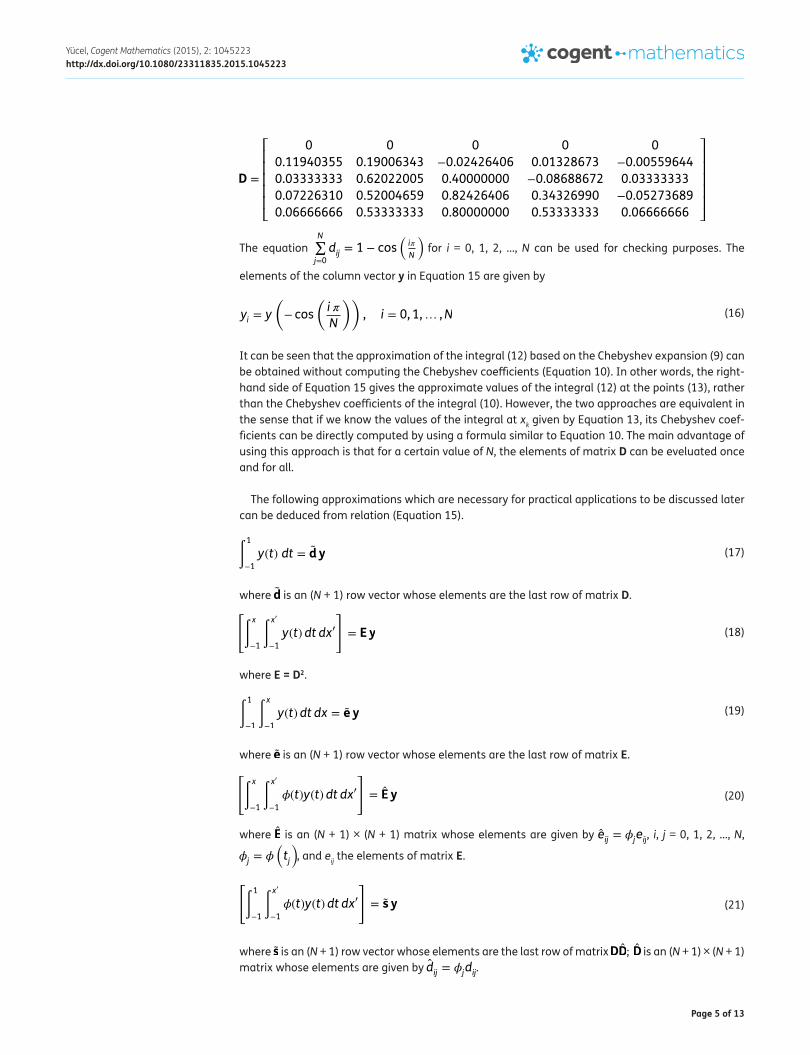
This can be achieved using modern computing tools like Maple and Matlab. For N = 4, the elements of the matrix D, obtained by Maple, are given below.

(9)y(x) =

N∑i=0

��aiTi(x)

(10)ai =2

N

N∑j=0

��y(xj)Ti(xj), i = 0, 1,… ,N

(11)xj = cos

(j�

N

), j = 0, 1,… ,N

(12)�x

−1

y(t)dt , −1 ≤ x ≤ 1

(13)xk = − cos

(k�

N

), k = 0, 1,… ,N

(14)∫x

−1

y(t)dt =

N∑k=0

��y(xk)2

N

N∑i=0

��Ti(xk) ∫x

−1

Ti(t)dt

(15)[∫x

−1

y(t)dt

]= D y

of 13


The equation N∑j=0

dij = 1 − cos�i�

N

� for i = 0, 1, 2, …, N can be used for checking purposes. The

elements of the column vector y in Equation 15 are given by

It can be seen that the approximation of the integral (12) based on the Chebyshev expansion (9) can be obtained without computing the Chebyshev coefficients (Equation 10). In other words, the right-hand side of Equation 15 gives the approximate values of the integral (12) at the points (13), rather than the Chebyshev coefficients of the integral (10). However, the two approaches are equivalent in the sense that if we know the values of the integral at xk given by Equation 13, its Chebyshev coef-ficients can be directly computed by using a formula similar to Equation 10. The main advantage of using this approach is that for a certain value of N, the elements of matrix D can be eveluated once and for all.

The following approximations which are necessary for practical applications to be discussed later can be deduced from relation (Equation 15).

where d is an (N + 1) row vector whose elements are the last row of matrix D.

where E = D2.

where e is an (N + 1) row vector whose elements are the last row of matrix E.

where E is an (N + 1) × (N + 1) matrix whose elements are given by eij = 𝜙jeij, i, j = 0, 1, 2, …, N,

�j = �

(tj

), and eij the elements of matrix E.

where s is an (N + 1) row vector whose elements are the last row of matrix DD; D is an (N + 1) × (N + 1) matrix whose elements are given by dij = 𝜙jdij.

D =

⎡⎢⎢⎢⎢⎢⎣

0 0 0 0 0

0.11940355 0.19006343 −0.02426406 0.01328673 −0.00559644

0.03333333 0.62022005 0.40000000 −0.08688672 0.03333333

0.07226310 0.52004659 0.82426406 0.34326990 −0.05273689

0.06666666 0.53333333 0.80000000 0.53333333 0.06666666

⎤⎥⎥⎥⎥⎥⎦

(16)yi = y

(− cos

(i �

N

)), i = 0, 1,… ,N

(17)∫1

−1

y(t) dt = d y

(18)

[∫x

−1∫x�

−1

y(t)dt dx�

]= E y

(19)∫1

−1∫x

−1

y(t)dt dx = e y

(20)

[∫x

−1∫x�

−1

𝜙(t)y(t)dt dx�

]= E y

(21)

[∫1

−1∫x�

−1

𝜙(t)y(t)dt dx�

]= s y

of 13


where H = D4.

where h is an (N + 1) row vector whose elements are the last row of matrix H.

Standard Chebyshev polynomials of the first kind Tr(x) are valid over the interval [−1, 1]. However, this interval can be normalized using the change of variable x → (x + 1)∕2. In this case, the Chebyshev expansion of the integral will be in terms of the shifted Chebyshev polynomials of the first kind defined by

which are valid over the interval [0, 1]. All the properties of T∗r (x) can be deduced from those of Tr(2x−1) (Fox & Parker, 1968). Therefore, when the range is [0, 1], we have the approximation

where D =1

2D and the right-hand side defines the integral at the grid points

The elements of the column y in Equation 25 are also defined at these points. Hence, for practical applications, the operators from Equations 18 to 23 can be similarly defined by replacing the matrix D by D and the points Equation 13 by Equation 26.

As can be seen from the above formulas, the range of x in the computational domain should either be [−1, 1] or [0, 1]. For practical applications, the physical domain is neither [−1, 1] nor [0, 1], but rather [a, b], then for this case, we can perform a coordinate transformation. This can be easily done by remembering that any finite range, a ≤ t ≤ b, can be transformed to the basic range −1 ≤ x ≤ 1 and/or the range 0 ≤ x ≤ 1 with the change of variables

3. Applications to SLPsIn this section, we consider the numerical approximations of second- and fourth-order Sturm–Liouville eigenvalues using the matrix representations of the integrals obtained above.

3.1. Second-order problemThe general SLP (1) can be easily reduced to the so-called Liouville normal form (or equivalently the Schrödinger equation)

(22)

[∫x

−1∫x�

−1∫x��

−1∫x��

−1

y(t)dt dx��dx�� dx�

]= Hy

(23)∫1

−1∫x

−1∫x�

−1∫x��

−1

y(t)dt dx��dx�dx = h y

(24)T∗r (x) = Tr(2x − 1), 0 ≤ x ≤ 1

(25)[∫x

0

y(t)dt

]= D y

(26)xk =1

2

[1 − cos

(k�

N

)], k = 0, 1,… ,N

(27)t =1

2

(b − a

)x +

1

2

(b + a

), t =

(b − a

)x + a

(28)−y��(t) + q(t) y(t) = 𝜆 y(t) , a < t < b

of 13


where now all the properties of the original equation can be associated with the properties of the coefficient q(∙) on the transformed interval

(a, b

). In this form, the properties of the original differ-

ential equation may be easier to consider for both analytical and numerical purposes. The endpoint classification at a, b of Equation 1 is invariant under the Liouville transformation and is identical with the endpoint classification at a, b. Therefore, we consider the above differential equation with the boundary conditions (4).

We first perform a coordinate transformation of the first form of Equation 27. Then, Equation 28 becomes

where q(x) =((b − a)∕2

)2q(x) and �� =

((b − a)∕2

)2𝜆. The boundary conditions, in this case, are

It should be noted that translating the equation from the t domain to the x domain leaves the eigen-values unaltered.

To apply the method developed in the previous section, we first integrate Equation 29 from the lower limit −1 to an arbitrary value of x ∈ [−1, 1] to obtain

Similarly, integrating the resulting Equation 31 once more yields

where we have made use of the boundary condition y(−1) = 0. In this equation, y′(−1) is an unknown that has to be determined by introducing boundary conditions (Equation 30). To do this, we first specialize Equation 32 for x = 1, together with the boundary conditions given by Equation 30. Then, we obtain

We can now substitute the so obtained y′(−1) into Equation 32 to obtain the final integrated form

Using the techniques developed in the previous section to calculate integrals, this integral equation can now be transformed into the following eigenvalue equation:

where A and B are (N + 1) × (N + 1) matrices whose entries are given by

(29)−y��(x) + q(x) y(x) = �� y(x) , −1 < x < 1

(30)y(−1) = 0, y(1) = 0

(31)−y�(x) + y�(−1) + ∫x

−1

q(t)y(t)dt = �� ∫x

−1

y(t)dt

(32)−y(x) + (x + 1)y�(−1) + ∫x

−1∫t

−1

q(t�)y(t�)dt�dt = �� ∫x

−1∫t

−1

y(t�)dt�dt

(33)y�(−1) = −1

2 ∫1

−1∫t

−1

q(t�)y(t�)dt�dt +��

2 ∫1

−1∫t

−1

y(t�)dt�dt

(34)

− y(x) −(x + 1)

2 ∫1

−1∫t

−1

q(t�)y(t�)dt�dt + ∫x

−1∫t

−1

q(t�)y(t�)dt�dt

= ��

[∫x

−1∫t

−1

y(t�)dt�dt −(x + 1)

2 ∫1

−1∫t

−1

y(t�)dt�dt

]

(35)Ay = ��By

(36)aij = −𝛿ij − uisj + eij , bij = eij − uiej , i, j = 0, 1, 2,… ,N

of 13


In the above equation, δij is the Kronecker delta, ui =(xi + 1

)∕ 2 the elements of an (N + 1) column

vector u, sj the elements of (N + 1) row vector s given by Equation 21 with 𝜙 = q, eij the elements of (N + 1) × (N + 1) matrix E given by Equation 20 with 𝜙 = q, eij the elements of (N + 1) × (N + 1) matrix E, and ej the elements of (N + 1) row vector e given by Equation 19. It should be noted that proper definition of Equation 36 can be easily obtained when the transformed range is [0, 1]. It is important to note that the first and last columns of B have no effect (since multuplied by zero). Hence, the eigenvalue Equation 35 can be reduced to a (N − 1) × (N − 1) system by eliminating the first and last rows and columns of matrices A and B.

Equation 35 is a generalized eigenvalue problem. When B is non-singular, this equation is

mathematically equivalent to (B-1A

)y = �� y, and when A is non-singular, it is equivalent to (

A-1B)y =

(1 ∕ ��

)y. Thus, in theory, if one of the matrices A or B is known to be non-singular, the

problem could be reduced to a standard eigenvalue problem. However, for this reduction to be satisfactory from the point of view of numerical stability, it is necessary not only that B (or A) should be non-singular, but that it should be well-conditioned with respect to inversion. There are many underlying computational routines that can be used for solving these problems. Once we have the computed �� values, they can be used to obtain the eigenvalues of the original problem (28) using 𝜆 = ��∕

((b − a)∕2

)2.

3.2. A simple case of the fourth-order problemAlthough the numerical results of Equation 3 with some specified end conditions, obtained using the solutions of the second-order problem, will be given in the next section, we consider here a simple case of Equation 3 to demonstrate directly the use of El-gendi’s method on the fourth-order prob-lems. Therefore, we put P(x) = W(x) = 1, S(x) = Q(x) = 0, a = 0, and b = 1 in Equation 3. Then, we obtain the following simple equation, the steady-state Euler-Bernoulli equation for the deflection y(x) of a vibrating beam of length 1:

As mentioned earlier, there are three types of boundary conditions and their combinations com-monly used with this equation in applications. In this work, the formulations are given only for one of them. Other types of boundary conditions can be handled similarly. We assume that the clamped end is at x = 0 and the simply supported end is at x = 1,

A coordinate transformation is not necessary for this case since the physical domain is already [0, 1]. By successive integration of Equation 37 from the lower limit 0 to an arbitrary value of x ∈ [0, 1], we obtain

(37)y(4)(x) = 𝜆 y(x), 0 < x < 1

(38)y(0) = y�(0) = 0, y(1) = y��(1) = 0

(39)y��(x) − y��(0) = � ∫x

0

y(t)dt

(40)y��(x) − y��(0) − x y��(0) = � ∫x

0∫x�

0

y(t)dtdx�

(41)y�(x) − xy��(0) −x2

2y��(0) = � ∫

x

0∫x�

0∫x��

0

y(t)dtdx��dx�

(42)y(x) −x2

2y��(0) −

x3

6y��(0) = � ∫

x

0∫x�

0∫x��

0∫x��

0

y(t)dtdx��dx��dx�

of 13


As can be seen from Equation 42, there are two unknowns, y′′(0) and y′′′(0), to be determined by introducing boundary conditions. Specializing Equations 40 and 42 for x = 1, together with the boundary conditions given by Equation 38, and then solving the resulting system of equations for the two unknowns, we obtain the final integrated form of Equation 42 as

Using the techniques developed in Section 2 to calculate integrals, this integral equation can be transformed into the following generalized eigenvalue equation:

where A and B are (N + 1) × (N + 1) matrices whose entries are given by

Here, vi =(x3i − 3x

2

i

)∕ 2 are the elements of an (N + 1) column vector v, zi =

(x2i − x

3

i

)∕ 4 the ele-

ments of an (N + 1) column vector z, hij the elements of (N + 1) × (N + 1) matrix H given by Equation 22, hj the elements of (N + 1) row vector h given by Equation 23, and ej the elements of (N + 1) row vector e given by Equation 19. For the same reason given in Section 3.1, the eigenvalue equation (44) can be reduced to a (N − 1) × (N − 1) system. A computational routine can now be used to solve Equation 44 for obtaining eigenvalues of the problem.

4. Numerical resultsWe present here the results obtained by applying our algorithms to the numerical solution of some second- and fourth-order SLPs in practice. First two problems which have exact solutions are chosen to demonstrate the efficiency and accuracy of the method developed in this work. We will use the relative error εk which is defined as

to measere the performance of the method. In the last problem, we choose the fourth-order prob-lem (3) to be square of the second-order problem (1) as discussed in Section 1. Numerical calcula-tions are carried out using Maple and Matlab.

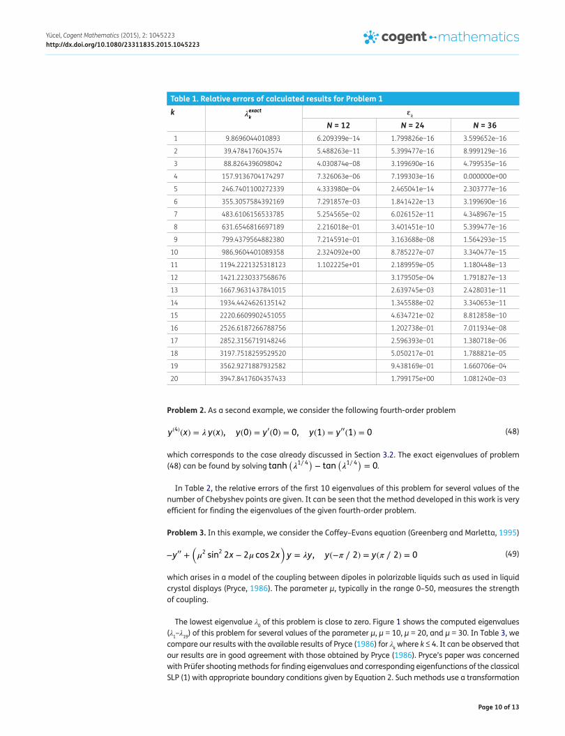
Problem 1. Our first example for the second-order SLP is given by

which arises when solving the one-dimensional wave equation utt−uxx = 0 (the standard model for an oscillating string of length 1 with fixed endpoints) using a “seperation of variables” method. The exact eigenvalues of this problem are �k = k

2�2, k = 1, 2, 3, … .

Table 1 lists the relative errors of the obtained results with different number of the Chebyshev points N. It is observed from this table that in order to have good approximations to the first kth eigenvalues, at least 2k Chebyshev points have to be used. It is also observed that the computed values for the lower eigenvalues have a better accuracy than those for the higher eigenvalues. As the number of grid points further increased to above 2k, the accuracy of the obtained results espe-cially for the higher eigenvalues can be further improved as shown in Table 1.

(43)

y(x) = �

[∫x

0∫x�

0∫x��

0∫x��

0

y(t)dtdx��dx��dx�

+

(x3 − 3x2

2

)∫1

0∫x�

0∫x��

0∫x��

0

y(t)dtdx��dx��dx� +

(x2 − x3

4

)∫1

0∫x

0

y(t)dtdx

]

(44)Ay = �By

(45)aij = 𝛿ij , bij = hij + vihj + ziej , i, j = 0, 1, 2,… ,N

(46)�k =

||||||�exactk − �

approx

k

�exactk

||||||, k = 1, 2, 3,… ,

(47)−y��(x) = �y(x), y(0) = y(1) = 0

of 13


Problem 2. As a second example, we consider the following fourth-order problem

which corresponds to the case already discussed in Section 3.2. The exact eigenvalues of problem (48) can be found by solving tanh

(�1∕ 4

)− tan

(�1∕ 4

)= 0.

In Table 2, the relative errors of the first 10 eigenvalues of this problem for several values of the number of Chebyshev points are given. It can be seen that the method developed in this work is very efficient for finding the eigenvalues of the given fourth-order problem.

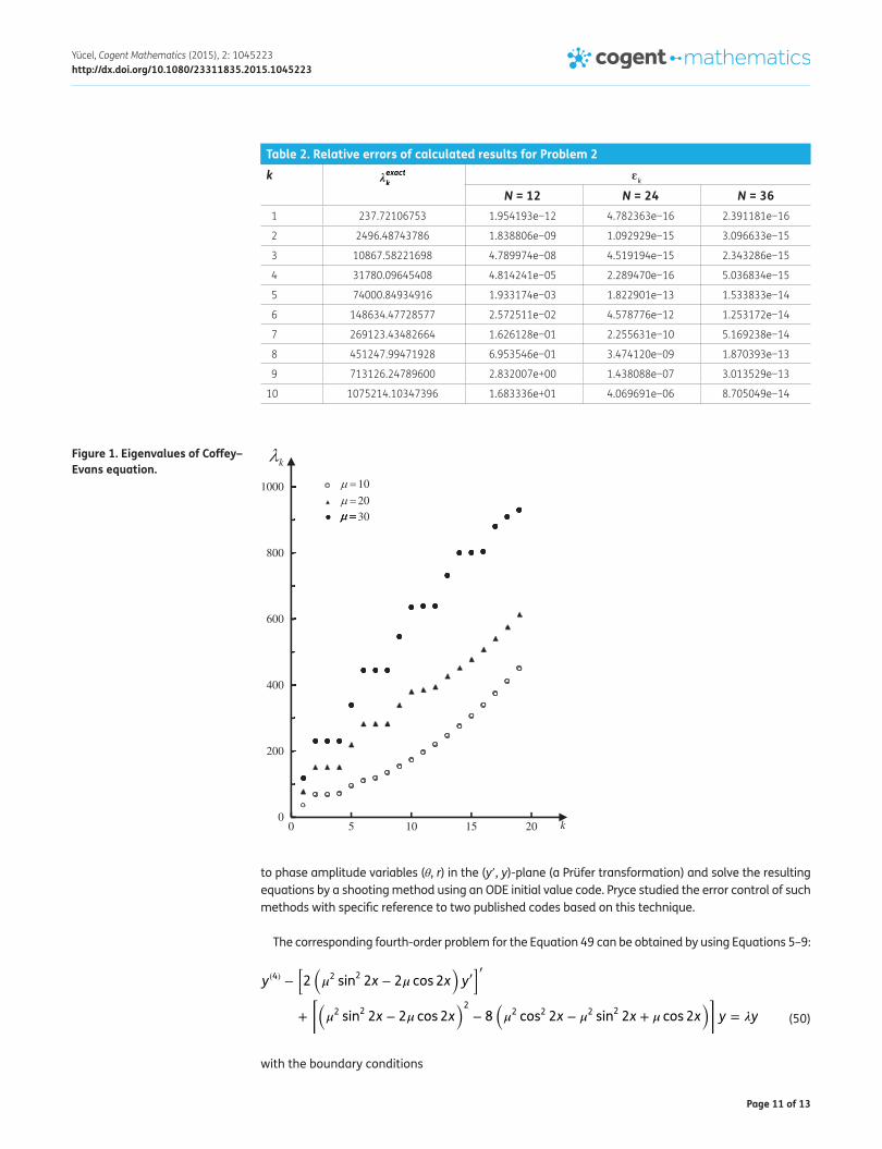
Problem 3. In this example, we consider the Coffey–Evans equation (Greenberg and Marletta, 1995)

which arises in a model of the coupling between dipoles in polarizable liquids such as used in liquid crystal displays (Pryce, 1986). The parameter μ, typically in the range 0–50, measures the strength of coupling.

The lowest eigenvalue λ0 of this problem is close to zero. Figure 1 shows the computed eigenvalues (λ1–λ19) of this problem for several values of the parameter μ, μ = 10, μ = 20, and μ = 30. In Table 3, we compare our results with the available results of Pryce (1986) for λk where k ≤ 4. It can be observed that our results are in good agreement with those obtained by Pryce (1986). Pryce’s paper was concerned with Prüfer shooting methods for finding eigenvalues and corresponding eigenfunctions of the classical SLP (1) with appropriate boundary conditions given by Equation 2. Such methods use a transformation

(48)y(4)(x) = � y(x), y(0) = y�(0) = 0, y(1) = y��(1) = 0

(49)−y�� +(�2 sin

22x − 2� cos 2x

)y = �y, y(−� ∕ 2) = y(� ∕ 2) = 0

Table 1. Relative errors of calculated results for Problem 1k �

exact

kɛk

N = 12 N = 24 N = 36 1 9.8696044010893 6.209399e−14 1.799826e−16 3.599652e−16

2 39.4784176043574 5.488263e−11 5.399477e−16 8.999129e−16

3 88.8264396098042 4.030874e−08 3.199690e−16 4.799535e−16

4 157.9136704174297 7.326063e−06 7.199303e−16 0.000000e+00

5 246.7401100272339 4.333980e−04 2.465041e−14 2.303777e−16

6 355.3057584392169 7.291857e−03 1.841422e−13 3.199690e−16

7 483.6106156533785 5.254565e−02 6.026152e−11 4.348967e−15

8 631.6546816697189 2.216018e−01 3.401451e−10 5.399477e−16

9 799.4379564882380 7.214591e−01 3.163688e−08 1.564293e−15

10 986.9604401089358 2.324092e+00 8.785227e−07 3.340477e−15

11 1194.2221325318123 1.102225e+01 2.189959e−05 1.180448e−13

12 1421.2230337568676 3.179505e−04 1.791827e−13

13 1667.9631437841015 2.639745e−03 2.428031e−11

14 1934.4424626135142 1.345588e−02 3.340653e−11

15 2220.6609902451055 4.634721e−02 8.812858e−10

16 2526.6187266788756 1.202738e−01 7.011934e−08

17 2852.3156719148246 2.596393e−01 1.380718e−06

18 3197.7518259529520 5.050217e−01 1.788821e−05

19 3562.9271887932582 9.438169e−01 1.660706e−04

20 3947.8417604357433 1.799175e+00 1.081240e−03

of 13


to phase amplitude variables (θ, r) in the (y′, y)-plane (a Prüfer transformation) and solve the resulting equations by a shooting method using an ODE initial value code. Pryce studied the error control of such methods with specific reference to two published codes based on this technique.

The corresponding fourth-order problem for the Equation 49 can be obtained by using Equations 5–9:

with the boundary conditions

(50)

y(4) −[2(�2 sin

22x − 2� cos 2x

)y�]�

+

[(�2 sin

22x − 2� cos 2x

)2− 8

(�2 cos2 2x − �

2 sin22x + � cos 2x

)]y = �y

Table 2. Relative errors of calculated results for Problem 2k �

exact

kɛk

N = 12 N = 24 N = 36 1 237.72106753 1.954193e−12 4.782363e−16 2.391181e−16

2 2496.48743786 1.838806e−09 1.092929e−15 3.096633e−15

3 10867.58221698 4.789974e−08 4.519194e−15 2.343286e−15

4 31780.09645408 4.814241e−05 2.289470e−16 5.036834e−15

5 74000.84934916 1.933174e−03 1.822901e−13 1.533833e−14

6 148634.47728577 2.572511e−02 4.578776e−12 1.253172e−14

7 269123.43482664 1.626128e−01 2.255631e−10 5.169238e−14

8 451247.99471928 6.953546e−01 3.474120e−09 1.870393e−13

9 713126.24789600 2.832007e+00 1.438088e−07 3.013529e−13

10 1075214.10347396 1.683336e+01 4.069691e−06 8.705049e−14

Figure 1. Eigenvalues of Coffey–Evans equation.

0

200

400

600

800

1000

30

0 5 10 15 20 k

k

3020

10

of 13


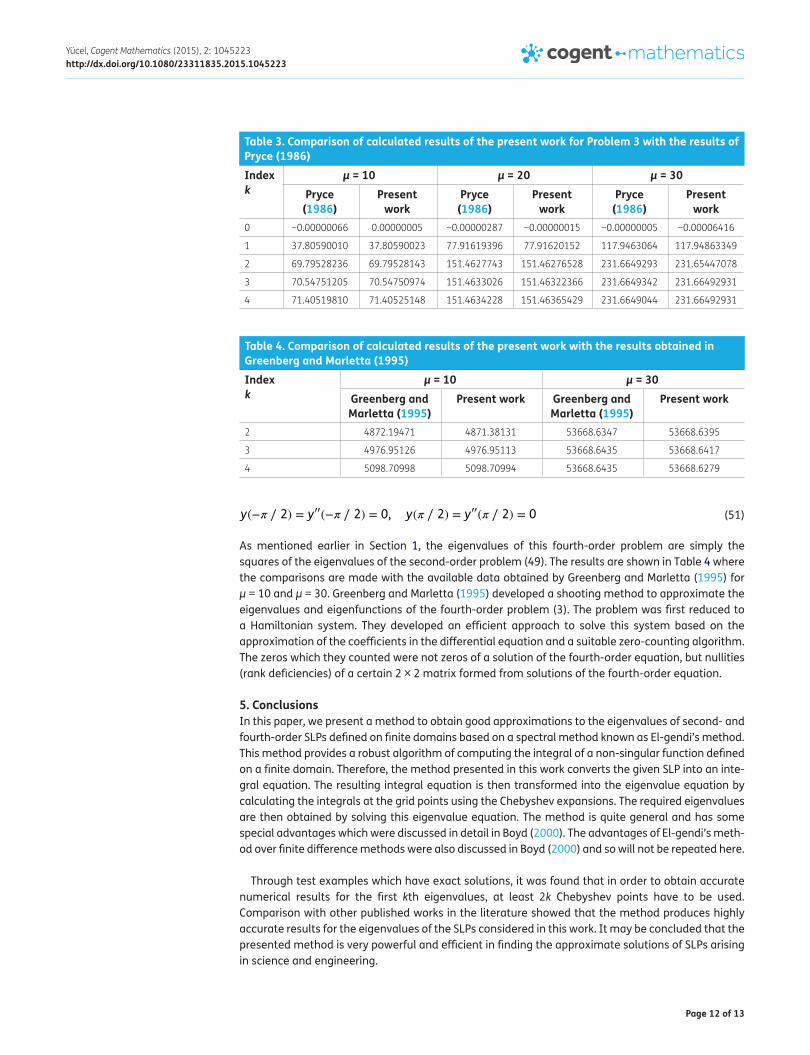
As mentioned earlier in Section 1, the eigenvalues of this fourth-order problem are simply the squares of the eigenvalues of the second-order problem (49). The results are shown in Table 4 where the comparisons are made with the available data obtained by Greenberg and Marletta (1995) for μ = 10 and μ = 30. Greenberg and Marletta (1995) developed a shooting method to approximate the eigenvalues and eigenfunctions of the fourth-order problem (3). The problem was first reduced to a Hamiltonian system. They developed an efficient approach to solve this system based on the approximation of the coefficients in the differential equation and a suitable zero-counting algorithm. The zeros which they counted were not zeros of a solution of the fourth-order equation, but nullities (rank deficiencies) of a certain 2 × 2 matrix formed from solutions of the fourth-order equation.

5. ConclusionsIn this paper, we present a method to obtain good approximations to the eigenvalues of second- and fourth-order SLPs defined on finite domains based on a spectral method known as El-gendi’s method. This method provides a robust algorithm of computing the integral of a non-singular function defined on a finite domain. Therefore, the method presented in this work converts the given SLP into an inte-gral equation. The resulting integral equation is then transformed into the eigenvalue equation by calculating the integrals at the grid points using the Chebyshev expansions. The required eigenvalues are then obtained by solving this eigenvalue equation. The method is quite general and has some special advantages which were discussed in detail in Boyd (2000). The advantages of El-gendi’s meth-od over finite difference methods were also discussed in Boyd (2000) and so will not be repeated here.

Through test examples which have exact solutions, it was found that in order to obtain accurate numerical results for the first kth eigenvalues, at least 2k Chebyshev points have to be used. Comparison with other published works in the literature showed that the method produces highly accurate results for the eigenvalues of the SLPs considered in this work. It may be concluded that the presented method is very powerful and efficient in finding the approximate solutions of SLPs arising in science and engineering.

(51)y(−� ∕ 2) = y��(−� ∕ 2) = 0, y(� ∕ 2) = y��(� ∕ 2) = 0

Table 3. Comparison of calculated results of the present work for Problem 3 with the results of Pryce (1986)Index k

μ = 10 μ = 20 μ = 30Pryce

(1986)Present

workPryce

(1986)Present

workPryce

(1986)Present

work0 −0.00000066 0.00000005 −0.00000287 −0.00000015 −0.00000005 −0.00006416

1 37.80590010 37.80590023 77.91619396 77.91620152 117.9463064 117.94863349

2 69.79528236 69.79528143 151.4627743 151.46276528 231.6649293 231.65447078

3 70.54751205 70.54750974 151.4633026 151.46322366 231.6649342 231.66492931

4 71.40519810 71.40525148 151.4634228 151.46365429 231.6649044 231.66492931

Table 4. Comparison of calculated results of the present work with the results obtained in Greenberg and Marletta (1995)Index k

μ = 10 μ = 30Greenberg and Marletta (1995)

Present work Greenberg and Marletta (1995)

Present work

2 4872.19471 4871.38131 53668.6347 53668.6395

3 4976.95126 4976.95113 53668.6435 53668.6417

4 5098.70998 5098.70994 53668.6435 53668.6279

of 13


© 2015 The Author(s). This open access article is distributed under a Creative Commons Attribution (CC-BY) 4.0 license.You are free to: Share — copy and redistribute the material in any medium or format Adapt — remix, transform, and build upon the material for any purpose, even commercially.The licensor cannot revoke these freedoms as long as you follow the license terms.

Under the following terms:Attribution — You must give appropriate credit, provide a link to the license, and indicate if changes were made. You may do so in any reasonable manner, but not in any way that suggests the licensor endorses you or your use. No additional restrictions You may not apply legal terms or technological measures that legally restrict others from doing anything the license permits.

AcknowledgmentsThe author would like to thank the editor and two anonymous referees for their valuable comments and suggestions to substantially improve the paper.

FundingThis work was supported by the Council of Higher Education of Turkey [Article 39 of Law No. 2547].

Author detailsUğur Yücel1

E-mail: [email protected] Faculty of Arts and Sciences, Department of Mathematics,

Pamukkale University, Denizli 20070, Turkey.

Citation informationCite this article as: Numerical approximations of Sturm–Liouville eigenvalues using Chebyshev polynomial expansions method, Uğur Yücel, Cogent Mathematics (2015), 2: 1045223.

ReferencesAmodio, P., & Settanni, G. (2015). Reprint of variable-step finite

difference schemes for the solution of Sturm–Liouville problems. Communications in Nonlinear Science and Numerical Simulation, 21, 12–21. http://dx.doi.org/10.1016/j.cnsns.2014.10.014

Amrein, W. O., Hinz, A. M., & Pearson, D. B. (2005). Sturm-Liouville theory. Basel: Birkhäuser Verlag. http://dx.doi.org/10.1007/3-7643-7359-8

Boyd, J. P. (2000). Chebyshev and Fourier spectral methods. New York, NY: Dover Publications.

El-gamel, M., & Abd El-hady, M. (2013). Two very accurate and efficient methods for computing eigenvalues of Sturm–Liouville problems. Applied Mathematical Modelling, 37, 5039–5046. http://dx.doi.org/10.1016/j.apm.2012.10.019

El-gendi, S. E. (1969). Chebyshev solution of differential, ıntegral and ıntegro-differential equations. The Computer Journal, 12, 282–287. http://dx.doi.org/10.1093/comjnl/12.3.282

Elliott, D. (1963). A Chebyshev series method for the numerical solution of Fredholm integral equations. The Computer Journal, 6, 102–112. http://dx.doi.org/10.1093/comjnl/6.1.102

Fox, L. (1962). Chebyshev methods for ordinary differential equations. The Computer Journal, 4, 318–331. http://dx.doi.org/10.1093/comjnl/4.4.318

Fox, L., & Parker, I. B. (1968). Chebyshev polynomials in numerical analysis. London: Oxford University Press.

Greenberg, L. (1991). An oscillation method for fourth-

order, selfadjoint, two-point boundary value problems with nonlinear eigenvalues. SIAM Journal on Mathematical Analysis, 22, 1021–1042. http://dx.doi.org/10.1137/0522067

Greenberg, L., & Marletta, M. (1995). Oscillation theory and numerical solution of fourth order Sturm–Liouville problems. IMA Journal of Numerical Analysis, 15, 319–356. http://dx.doi.org/10.1093/imanum/15.3.319

Khater, A. H., & Temsah, R. S. (2008). Numerical solutions of the generalized Kuramoto–Sivashinsky equation by Chebyshev spectral collocation methods. Computers & Mathematics with Applications, 56, 1465–1472. http://dx.doi.org/10.1016/j.camwa.2008.03.013

Mihaila, B., & Mihaila, I. (2002). Numerical approximations using Chebyshev polynomial expansions: El-gendi’s method revisited. Journal of Physics A: Mathematical and General, 35, 731–746. http://dx.doi.org/10.1088/0305-4470/35/3/317

Pryce, J. D. (1986). Error control of phase-function shooting methods for Sturm–Liouville problems. IMA Journal of Numerical Analysis, 6, 103–123. http://dx.doi.org/10.1093/imanum/6.1.103

Pryce, J. D. (1993). Numerical solution of Sturm–Liouville problems. Oxford: Oxford University Press.

Saleh Taher, A. H., Malek, A., & Momeni-Masuleh, S. H. (2013). Chebyshev differentiation matrices for efficient computation of the eigenvalues of fourth-order Sturm–Liouville problems. Applied Mathematical Modelling, 37, 4634–4642. http://dx.doi.org/10.1016/j.apm.2012.09.062

Temsah, R. S. (2009). Numerical solutions for convection-diffusion equation using El-Gendi method. Communications in Nonlinear Science and Numerical Simulation, 14, 760–769. http://dx.doi.org/10.1016/j.cnsns.2007.11.004

Yuan, S., Ye, K., Xiao, C., Kennedy, D., & Williams, F. W. (2014). Solution of regular second- and fourth-order Sturm–Liouville problems by exact dynamic stiffness method analogy. Journal of Engineering Mathematics, 86, 157–173. http://dx.doi.org/10.1007/s10665-013-9646-5

Yücel, U. (2006). Approximations of Sturm–Liouville eigenvalues using differential quadrature (DQ) method. Journal of Computational and Applied Mathematics, 192, 310–319. http://dx.doi.org/10.1016/j.cam.2005.05.008

Yücel, U., & Boubaker, K. (2012). Differential quadrature method (DQM) and Boubaker polynomials expansion scheme (BPES) for efficient computation of the eigenvalues of fourth-order Sturm–Liouville problems. Applied Mathematical Modelling, 36, 158–167. http://dx.doi.org/10.1016/j.apm.2011.05.030

mailto:[email protected]

http://dx.doi.org/10.1016/j.cnsns.2014.10.014


http://dx.doi.org/10.1007/3-7643-7359-8

http://dx.doi.org/10.1007/3-7643-7359-8

http://dx.doi.org/10.1016/j.apm.2012.10.019

http://dx.doi.org/10.1093/comjnl/12.3.282





http://dx.doi.org/10.1137/0522067

http://dx.doi.org/10.1137/0522067

http://dx.doi.org/10.1093/imanum/15.3.319


http://dx.doi.org/10.1016/j.camwa.2008.03.013

http://dx.doi.org/10.1016/j.camwa.2008.03.013

http://dx.doi.org/10.1088/0305-4470/35/3/317

http://dx.doi.org/10.1088/0305-4470/35/3/317






http://dx.doi.org/10.1007/s10665-013-9646-5

http://dx.doi.org/10.1016/j.cam.2005.05.008



Numerical approximations of Sturm–Liouville … using Chebyshev polynomial expansions method Uğur...

Documents

Transcript of Numerical approximations of Sturm–Liouville … using Chebyshev polynomial expansions method Uğur...