1 “Introduction and Mathematics Revision”

1 “Introduction and

Mathematics Revision”

Signal Analysis

J. A. M. Felippe de SouzaJ. A. M. Felippe de Souza

When we talk about signals generally it is associated with a measurement of some physical phenomenon or, in other words, of a system.

Therefore, signals and systems are concepts very interconnected.

Signal Analysis – Introduction______________________________________________________________________________________________________________________________________________________________________________________

(input) (output)


When one speaks of signals it is usually associated with the measurement or recording of some physical phenomenon or, in other words, of a system.

Therefore, signals and systems are very interconnected concepts


In this first chapter we will briefly review several basic topics of mathematics that will be useful for subsequent chapters.

We will summarize various results, expressions and formulas

of Algebra,

of Linear Algebra,

of Analysis,

of Differential and Integral Calculus

of Trigonometry

which will be somewhat used in this text.

In chapters 2 and 3 we will deal with the description and terminology of signals, while in chapter 4 we will deal with systems.

In the remaining chapters we will deal with some signal analysis tools:

Laplace Transforms (chapter 5),

z-Transforms (chapter 6),

Fourier Series and Transforms (chapters 7 e 8), and

Diagrams de Bode (chapter 9).

Signal Analysis – Mathematics Revision______________________________________________________________________________________________________________________________________________________________________________________

1j −=

The imaginary number “ j ” In Math literature it is very common to use “ i ”

(of “imaginary”) to a imaginary number:

1i −=However, in engineering the letter “ i ” is usually reserved for the electric

current (measured in Ampères) while for the imaginary number we use the letter “ j ”

1j2 −=1j3 −−=

1j4 =

1jjjj 145 −==⋅=

1jjjj 2246 −==⋅=

and so on.1jjjj 3347 −−==⋅=

111jjj 448 =⋅=⋅=

j)1(

j

jj

j

j

1j 1 −=

−=

⋅==−

1j 2 −=−

jj 3 =−

1j 4 =−


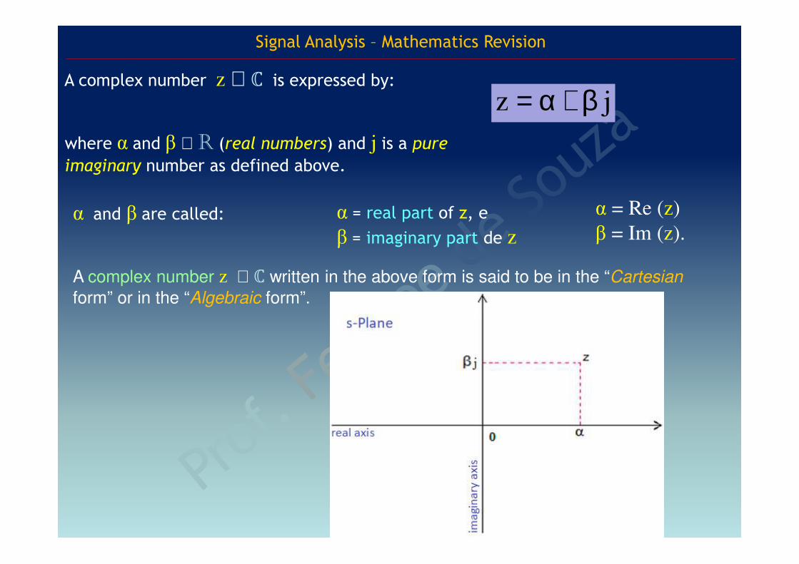
A complex number z ∈ ℂ is expressed by:

jz β+α=where α and β ∈ R (real numbers) and j is a pure

imaginary number as defined above.

α and β are called: α = real part of z, e

β = imaginary part de z

α = Re (z) β = Im (z).

A complex number z ∈ ℂ written in the above form is said to be in the “Cartesian

form” or in the “Algebraic form”.


A complex number z ∈ ℂ can be written equivalently as:

θ⋅ρ= jz ewhere ρ and θ are real numbers, with ρ > 0and θ (in radians) is an arc.

The above expression is very commonly abbreviated (especially in engineering texts) to

θ∠⋅ρ=z for the sake of simplicity.

ρ and θ are called:

Moreover, in this case, when using this

notation for z, it is common to denote

the angle θ in degrees instead of radians.

ρ = absolute value of z, and

θ = angle or phase of z

ρ = |z|

θ = ∠z

The complex number z written in this

form above is said to be in the “polar form” or “trigonometric form”.


Transformation from Cartesian form to polar form

22|z| β+α==ρ

=∠=αβθ arctgz

Transformation from polar form to Cartesian form

θ⋅ρ==α cos)zRe( θ⋅ρ==β sen)zIm(

)7854,0(j

)4/(j

2

8284,2

22

º31522

º4522

j22z

−

π−

⋅=⋅=

∠=

−∠=

−=

e

e


The conjugate of a complex number z ∈ ℂ jz β+α=is the complex number or z *z

z z* j= = α − βIn terms of the polar form the conjugate of a complex number

θ⋅ρ= jz e

is given by:

Note that

* *z (z ) z= =

in addition, if x is a real number (x ∈ R),

that is, x is a complex number with the

imaginary part equal to zero, then:

* *x (x ) x= =

θ−⋅ρ== j*zz e


Operations with complex numbers

The Cartesian form is more appropriate for sum operations (z1 + z2) as

well as the subtraction operations (z1 – z2) of complex numbers:

( ) ( ) ( ) ( ) jjj 21212211 ⋅β+β+α+α=⋅β+α+⋅β+α

( ) ( ) ( ) ( ) jjj 21212211 ⋅β−β+α−α=⋅β+α−⋅β+α

while the polar form is more appropriate for the operations of

multiplication (z1 ⋅ z2) and division (z1 / z2) of complex numbers:

( ) ( ) ( )2121 j21

j2

j1

θ+θ⋅θθ ⋅ρ⋅ρ=⋅ρ⋅⋅ρ eee

( )( )

( )21

2

1j

2

1j

2

j1 θ−θ⋅

θ

θ

⋅ρρ=

⋅ρ⋅ρ

ee

e

or, equivalently:

( ) ( ) )( 2121j

2j

121 θ+θ∠⋅ρ⋅ρ=⋅ρ⋅⋅ρ θθ

ee

( )( ) )( 21

2

1j

2

j1

2

1

θ−θ∠⋅ρρ=

⋅ρ⋅ρ

θ

θ

e

e


A very useful result is given by the equation below:

( ) ( ) 22jj β+α=β−α⋅β+αthat is, the product of a complex number z by its conjugate is a real number (a

complex number without the imaginary part) and whose value is the sum of the

square of the real part of z with the square of the imaginary part of z.

BjAj

j

z

z ⋅+=ω+σβ+α=

′

This result allows you to write a fraction between complex numbers either in

Cartesian form A + j⋅B, that is,

( )( )( )( )

( ) ( )22

j

jj

jj

zz

zz

z

z

ω+σαω−βσ⋅+βω+ασ=

ω−σω+σω−σβ+α=

′′′

=′

( )( )

( )( )2222

jz

z

ω+σαω−βσ⋅+

ω+σβω+ασ=

′

( )( )22

Aω+σβω+ασ=

( )( )22

Bω+σαω−βσ=

and therefore,

In other words, by multiplying both the numerator and the denominator

of z/z’ by the conjugate of the denominator we have:


Another very useful result is the following: θ∀=θ ,1je

that is, is a point on the circumference of radius 1 centred on the originof the s plane.

θ= jz e

10j =e

j2j

=π

e

1j −=πe

j2j

−=π−

e

is the point of this circumferencewhose angle to the positive

real axis is θ.

In fact

θ= jz e


The sine and the co-sine

Pythagorean theorem

222 cba +=

The tangent


( ) 1)(cossen 22 =θ+θ

π+θ=

θ−π=θ2

sen2

sen)(cos

( )

π−θ=θ2

cossen

( ) ( )θ−π=θ sensen

( ) ( )θ−π−=θ coscos

( ) ( )θ−−=θ sensen

( ) ( )θ−=θ coscos

co-sine

sine


tangent

( ) ( ) ( )π−θ=π+θ=θ tgtgtg

( ) ( ) { }...,2,1,0k,ktgtg ±±∈π+θ=θ


Euler’s equation

θ⋅+θ=θ senjcosje

2cos

jj θ−θ +=θ ee

j2sen

jj θ−θ −=θ ee

The Swiss mathematician and physicist Leonhard Euler (1707-1783) published the following result in 1748:

and we can easily obtain:


The inverse functions of sine, cosine, and tangent

The sine, cosine, and tangent functions are not invertible.

α ∈[–1, 1], β ∈[–1, 1], γ ∈(–∞, ∞),

and then there will be many values of t∈(–∞, ∞) for which

In order to find the inverse function of sine, cosine and tangent we have to limit the interval of these functions.

x(t) = sin (ωt) = α x(t) = cos (ωt) = β x(t) = tg (ωt) = γ

In the case of the sine we limit the interval t∈[–π/2 , π/2],

in the cosine case we limit the interval t∈[0 , π],

and in the case of the tangent we limit the interval t∈[–π/2 , π/2].

By the graphics of x(t) = sin (ωt), x(t) = cos (ωt) and x(t) = tg (ωt) we see that

α and β are values in the range [–1, 1], e γ for any real value, that is,


sine, co-sine and tangent with their limited intervals

This is the general rule adopted by calculating machines and modern computing means. The arc is limited to 2 quadrants:

1st and 4th quadrant, in the case of sine and also of tangent; and 1st and 2nd quadrant, in the case of co-sine.

In this way it is possible to speak in the inverse functions: of sine, co-sine and tangent:

arcsin (α), arccos (β) and arctg (γ).


For example, if γ = 1 ( ) º454

1arctg =π=Although there are many others arcs θwhose tangent is also 1.

º225eº45 =θ=θIn the particular case of the inverse

of a fraction (b/a)

arcsin (b/a),arccos (b/a) and

arctg (b/a)

then we can take into account the

quadrant of the point (a, b).

In this way the inverse of sine,

cosine or tangent is not limited to

the interval [–π/2 , π/2] or [0 , π]

which represent only 2 quadrants,

since we have enough information

to determine the arc in the 4

quadrants.


º4541

1tgarc =π=

º135º2254

5

1

1tgarc −==π=

−−

º315º4541

1tgarc =−=π−=

−

º1354

3

1

1tgarc =π=

−

(1st quadrant)

(3rd quadrant)

(4th quadrant)

(2nd quadrant)

For example:


More precisely, it can be written as an infinite series or as a boundary (the latter form due to the Swiss mathematician Jakob Bernoulli, 1654-1705):

Exponentials and logarithms

The “Neperian number” e (due to the mathematician, astrologer and Scottish

theologian John Napier, 1550-1617) is worth approximately e = 2.7183

∞

=

=0n !n

1e

n

n

11lim

n

+=∞→

e

The “Neperian number” e is also called the “Euler constant” and is the basis of

natural logarithms (ln). ( ) xxln =e

Some basic relations of exponentials and logarithms:

yxyx +=⋅ eee yx

y

x−= e

e

e ( ) yxyx ⋅= ee


Transformation of the base e to base 10:

( ) ( )( )

( ) ( )xln4343,03,2

xln

10ln

xlnxlog10 ⋅===

Transformation of the base 10 to base e:

( ) ( )( )

( ) ( )xlog3,24343,0

xlog

log

xlogxln 10

10

10

10 ⋅===e

Transformation from any base “b” to base “a”:

( ) ( )( )alog

xlogxlog

b

ba =

( ) ( ) ( )ylnxlnyxln +=⋅ ( ) ( )ylnxlny

xln −=

( ) ( )xlnaxln a =

( ) ( )x

1xx /1lnln ==−ee

Some basic relations of exponentials and logarithms:


Derivatives

The theory of differential calculus was created by the English physicist and mathematician

Sir Isaac Newton (1643-1727) and the German philosopher and mathematician

Gottfried Wilhelm von Leibniz (1646-1716).

The notation of the derivatives of a

function f(t) can bedt

df(due to Newton)

)t('f (due to Leibniz)

The derivative of a function f(t) at time t gives us the slope of a line tangent to the

curve at that instant.

Se f(t) is increasing in t = a, then the derivative will be positive in that instant

0>dt

df)a('f

at=

=

On the other hand, if f(t) is decreasing in t = a, then the derivative will be negative

in that instant

0<dt

df)a('f

at==


Negative slope of the tangent line to the

curve f(t) at the instant t = a.

Positive slope of the tangent line to the



Inclinação nula (ou declive nulo) da reta

tangente à curva f(t) no instante t = a.

Inflection point case, neither local maximum nor local minimum.

Zero slope of the tangent line to the


Case of local maximum or minimum.


Some Properties and Rules of Derivatives:

Linearity: ( ))t('fc

dt

)t(dfc

dt

)t(fcd ⋅=⋅=⋅

( ))t('f)t('f

dt

)t(df

dt

)t(df

dt

)t(f)t(fd21

2121 +=+=+

(homogeneity)

(additivity)

Product rule:

( ) )t(f)t('g)t(g)t('fdt

)t(dg)t(f)t(g

dt

)t(df)t(g)t(f

dt

d ⋅+⋅=⋅+⋅=⋅

Quotient rule:

)t(g

)t('g)t(f)t('f)t(g

)t(gdt

)t(dg)t(f

dt

)t(df)t(g

)t(g

)t(f

dt

d22

⋅−⋅=⋅−⋅

=

Chain rule:

( ) )t('g))t(g('fdt

)t(dg)t(g

dt

df))t(g(f

dt

d ⋅=⋅=


If we define

)t(f)t(u = and

and

)t(g)t(v =then,

udt

df ′= vdt

dg ′=

and the above rules can be rewritten in a compact form as:

( ) ucuc ′⋅=′⋅ (homogeneity)

( ) vuvu ′+′=′+ (additivity)

( ) vuvuvu ′⋅+⋅′=′⋅ (Product rule)

2v

vuuv

v

u ′⋅−′⋅=′

(Quotient rule)

dt

dv

dv

du

dt

du ⋅= (Chain rule)

Signal Analysis – Mathematics Revision ______________________________________________________________________________________________________________________________________________________________________________________

Integrals

The indefinite integral of a function f(t) is represented as τ⋅τ d)(f

On the other hand, the definite integral, represented as

τ⋅τb

ad)(f ∞−

τ⋅τb

d)(f ∞

τ⋅τa

d)(f

does the Riemann Sum calculating the area under the curve at a well-defined interval.

Georg Friedrich Bernhard Riemann (1826-1866), the German mathematician

The integral is an inverse process of the derivative of functions since,

( ) ( ) Ctfdfdtdt

)t(dfdt)t(

dt

dfdttf +====′

( ) )t(fdt)t(fdt

d =⋅or


This result is called the Fundamental Theorem of Calculus and makes the inter-connection between Differential and Integral Calculus.

More precisely : ⋅=

t

adt)t(f)t(F is called the primitive of f(t).

Some rules of integration of functions in general

( ) ( ) Cdttfadttfa +⋅=

( ) ( )[ ] ( ) ( ) Cdttgdttfdttgtf ++=+

( ) ( )[ ] ( ) ( ) ′⋅+⋅=⋅′ dttg)t(f)t(gtfdttgtf (integral by parts)

(additivity)

(homogeneity)

If we define )t(g)t(u = and

and

)t(f)t(v =

then, dt)t(gdu ⋅′= dt)t(fdv ⋅′=


and the rule of integral by parts can be written in another form:

−=⋅ duvuvdvu (integral by parts rule)

On the other hand, if

)t(f)t(u = e dt)t(fdu ⋅′=

then the definite integral is calculated as ] )a(u)b(uudu

ba

b

a−==

The integral defined from a to bof the function f

Sd)(fb

a=τ⋅τ

is the area S under the curve


Two examples of the integral defined from a to b f the function f, where areas below

the abscissa axis count negatively.

21

b

a1 SSd)(f −=τ⋅τ 321

b

a2 SSSd)(f +−=τ⋅τ


Two examples of the integral defined in infinite intervals such as: ( –∞, b] or [ a, ∞ ).

'Sd)(fb

3 =τ⋅τ ∞− ''Sd)(fa 4 =τ⋅τ∞


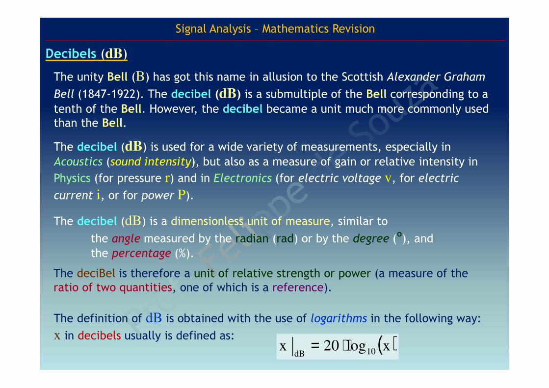
Decibels (dB)

The unity Bell (B) has got this name in allusion to the Scottish Alexander Graham

Bell (1847-1922). The decibel (dB) is a submultiple of the Bell corresponding to a

tenth of the Bell. However, the decibel became a unit much more commonly used than the Bell.

The decibel (dB) is used for a wide variety of measurements, especially in

Acoustics (sound intensity), but also as a measure of gain or relative intensity in

Physics (for pressure r) and in Electronics (for electric voltage v, for electric

current i, or for power P).

The decibel (dB) is a dimensionless unit of measure, similar to

the angle measured by the radian (rad) or by the degree (º), and

the percentage (%).

The deciBel is therefore a unit of relative strength or power (a measure of the ratio of two quantities, one of which is a reference).

The definition of dB is obtained with the use of logarithms in the following way:

x in decibels usually is defined as: ( )xlog20x 10dB⋅=


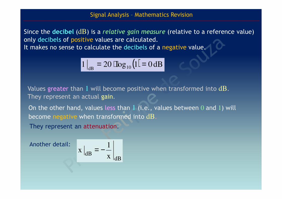
Since the decibel (dB) is a relative gain measure (relative to a reference value) only decibels of positive values are calculated.It makes no sense to calculate the decibels of a negative value.

( ) dB01log201 10dB=⋅=

Another detail:

dBdB x

1x −=

Values greater than 1 will become positive when transformed into dB.

They represent an actual gain.

On the other hand, values less than 1 (i.e., values between 0 and 1) will

become negative when transformed into dB.

They represent an attenuation.


if x 1>

if x 1=

if 0 < x < 1

if x < 0

dB x > 0dB

dB x 0dB=

dB x < 0dB

dBdoes not exist x

Some examples:

( ) dB2010log2001 10dB=⋅=

( ) ( ) ( ) dB2010log20110log201,010

110

110dB

dB

−=⋅⋅−=⋅== −

( ) dB4010log2010100 210dB

2

dB=⋅==

dB65,0dB

−=dB62dB

=

dB32dB

= dB32

1

dB

−=

dB46200 dB= dB142,0dB

−= dB3450 dB=


Obrigado!

Felippe de [email protected]

Thank you!

Departamento de Engenharia Eletromecânica

1 “Introduction and Mathematics Revision”

Documents

Transcript of 1 “Introduction and Mathematics Revision”