THOMAS WHITHAM SIXTH FORM

Additional Mathematics

Revision Guide

S J Cooper

The book contains a number of worked examples covering the topics needed in the Additional

Mathematics Specifications. This includes Calculus, Trigonometry, Geometry and the more advanced

Algebra. Plus the topics required for Mechanics and statistics.

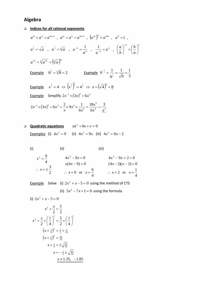
Algebra

Indices for all rational exponents

nmnm aaa , nmnm aaa , mnnm aa , 10 a ,

aa 2

1

, n aa n 1

, n

n

aa

1 , n

na

a

1 ,

nn

a

b

b

a

n maa nm

mn a

Example 288 33

1

Example 3

1

9

1

9

19

2

1

2

1

Example 43

2

x 2

32

3

3

2

4x 843

x

Example Simplify 321 632 xxx

24

2

3

2321 3

6

18

6

19

2632

xx

x

xx

xxxx

Quadratic equations 02 cbxax

Examples (i) 94 2 x (ii) xx 94 2 (iii) 294 2 xx

(i) (ii) (iii)

2

3

4

92

x

x

4

9or 0

0)94(

094 2

xx

xx

xx

4

1or 2

0)2)(14(

0294 2

xx

xx

xx

Example Solve (i) 052 2 xx using the method of CTS

(ii) 0175 2 xx using the formula.

(i) 052 2 xx

85.1 ,35.1

4

1

2

5

4

1

2

2

5

2

1641

41

1641

41

16412

41

161

252

41

22

2

2

x

x

x

x

x

xx

xx

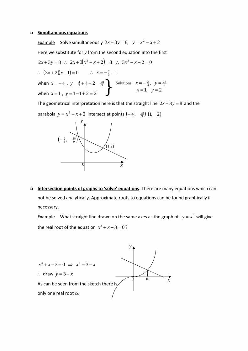
Simultaneous equations

Example Solve simultaneously 2 ,832 2 xxyyx

Here we substitute for y from the second equation into the first

832 yx 8232 2 xxx 023 2 xx

0123 xx 1 ,32x

when 32x ,

928

32

94 2 y

when 1x , 2211 y

The geometrical interpretation here is that the straight line 832 yx and the

parabola 22 xxy intersect at points 928

32 , 2,1

Intersection points of graphs to ‘solve’ equations. There are many equations which can

not be solved analytically. Approximate roots to equations can be found graphically if

necessary.

Example What straight line drawn on the same axes as the graph of 3xy will give

the real root of the equation 033 xx ?

033 xx xx 33

draw xy 3

As can be seen from the sketch there is

only one real root .

x

y

(1,2)

0

928

32 ,

} Solutions, 928

32 , yx

2 ,1 yx

x

y

0

Expansions and factorisation –extensions

Example

3732

3

622312

23

2

232

xxx

xx

xxxxxx

Expanding

Example 3399 23 xxxxxxx Factorising

The remainder Theorem

If the polynomial )(xp be divided by bax the remainder will be abp

Example When 532)( 3 xxxp is divided by 12 x the remainder is

4

1523

41

21 5 p

Example Find the remainder when 4𝑥3 − 3𝑥2 + 11𝑥 − 2 is divided by 𝑥 − 1.

1021111314123

f remainder is 10

The factor theorem Following on from the last item

baxpab 0 is a factor of )(xp

Example Show that 2x is a factor of 2136 23 xxx and hence solve the

equation 02136 23 xxx

Let 2136)( 23 xxxxp

02252482221326)2(23

p

2x is a factor of )(xp

162)( 2 xxxxp …by inspection

12132 xxx

Solutions to the equation are 21

31 , ,2 x

Expansion of nba where n is a positive integer.

This has the same coefficients as the expansion of nx1 . Each term will have degree

n, powers of a descending from na

Example .......28811 28 xxx

.......288 26788 babaaba

The general term will be rrn

r

n baC

Example

Use the binomial theorem to expand 423 x , simplifying each term of your expansion.

c

Gradient = m (= tan )

x

y

0

4322344464 babbabaaba

43223442234236234323 xxxxx

432 169621621681 xxxx

Geometry

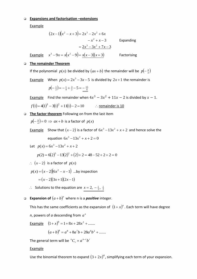
Gradient/ intercept form of a straight line Equation cmxy

Distance between two points

Given A 11, yx B 22 , yx then

2

12

2

12

2 yyxxAB

Gradient of a line through two points… 11, yxA and 22 , yxB say

12

12

xx

yym

Equation of a line through (x’, y’) of gradient m

xxmyy

Equation of a line through two points

Find the gradient using 12

12

xx

yym

and use the formula as above.

Parallel and perpendicular lines

Let two lines have gradients 1m and 2m

Lines parallel 21 mm

Lines perpendicular 121 mm or 2

1

1

mm

Mid-point of line joining … 11, yxA and 22 , yxB coordinates are

2121

2121 , yyxx

General form of a straight line

.0 cbyax To find the gradient, rewrite in gradient/intercept form.

Example Given points 3,2A and 1,1 B find

(a) distance AB

(b) the coordinates of the mid-point M of AB

(c) the gradient of AB

(d) the equation of the line through 2,5C parallel to AB

(a) 251693121222 AB AB = 5

(b) 1,21M

(c) Gradient AB = 3

4

21

31

(d) Point 2,5 Gradient = 34

Equation 5234 xy

2643

20463

xy

xy

Example Find the gradient of the line 1232 yx and the equation of a

perpendicular line through the point 4,0

1232 yx 1223 xy 432 xy grad =

32

Gradient of perpendicular =23

32

1

Equation 423 xy cmxy

The Circle

Angles in semicircle is 90

Perpendicular to a chord from centre of circle bisects the

chord.

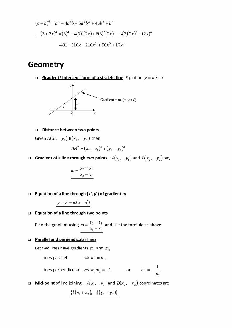
Centre, radius form of equation

222rbyax

Centre (a, b) radius = r

Example Centre (2, -1) radius 3 equation 91222 yx

Example Centre (1, 2) touching 0x Equation 42122 yx

General form of equation

222rbyax Circle centre 𝑎, 𝑏 with radius 𝑟

To find centre and radius, use the method of CTS to change into centre/radius form.

Example 033222 yxyx

4252

232

2

232

2322

22

22

1

13312

332

0332

yx

yyxx

yyxx

yxyx

Centre 23,1 radius =

25

Tangents

Angle between tangent and radius drawn to point of contact is

90

Tangents drawn from extended point

0

(1, 2)

Line of symmetry

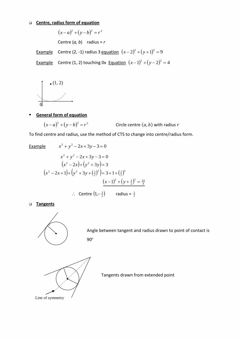
Example Find the equation of the tangent to the circle 054222 yxyx at

the point P(2, 1)

1021

4154412

542

0542

22

22

22

22

yx

yyxx

yyxx

yxyx

Centre at 2 ,1 , radius 10

Calculus

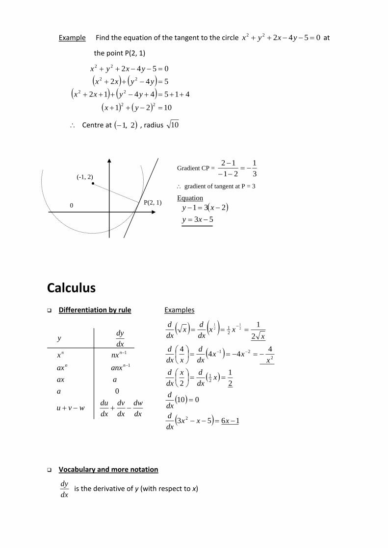
Differentiation by rule Examples

1653

010

2

1

2

444

4

2

1

2

21

2

21

21 2

1

2

1

xxxdx

d

dx

d

xdx

dx

dx

d

xxx

dx

d

xdx

d

xxx

dx

dx

dx

d

Vocabulary and more notation

dx

dy is the derivative of y (with respect to x)

dx

dw

dx

dv

dx

duwvu

a

aax

anxax

nxx

dx

dyy

nn

nn

0

1

1

0

(-1, 2)

P(2, 1)

Gradient CP = 3

1

21

12

gradient of tangent at P = 3

Equation

53

231

xy

xy

+ _

+ _

+

+

_

_

dx

dy is the differential coefficient of y (with respect to x).

Example 𝑦 = 𝑥3 − 4𝑥2 + 3𝑥 − 1

𝑑𝑦

𝑑𝑥= 3𝑥2 − 8𝑥 + 3

Example 2

1

2

3

222

)(22

xxxx

x

x

xxf

xx

xx

xxxxf1

2

312)(

2

3

2

1

2

3

2

1

23

21

23

The gradient of a curve at any point is given by the value of dx

dy at that point.

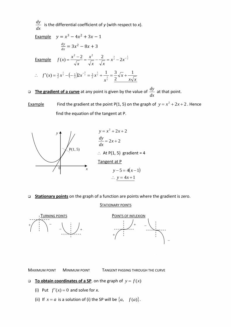
Example Find the gradient at the point P(1, 5) on the graph of 222 xxy . Hence

find the equation of the tangent at P.

22

222

xdx

dy

xxy

At P(1, 5) gradient = 4

Tangent at P

14

145

xy

xy

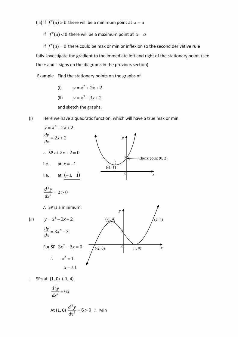
Stationary points on the graph of a function are points where the gradient is zero.

STATIONARY POINTS

TURNING POINTS POINTS OF INFLEXION

MAXIMUM POINT MINIMUM POINT TANGENT PASSING THROUGH THE CURVE

To obtain coordinates of a SP. on the graph of )(xfy

(i) Put 0)( xf and solve for x.

(ii) If ax is a solution of (i) the SP will be )(, afa .

P(1, 5)

0 x

y

(iii) If 0)( af there will be a minimum point at ax

If 0)( af there will be a maximum point at ax

If 0)( af there could be max or min or inflexion so the second derivative rule

fails. Investigate the gradient to the immediate left and right of the stationary point. (see

the + and - signs on the diagrams in the previous section).

Example Find the stationary points on the graphs of

(i) 222 xxy

(ii) 233 xxy

and sketch the graphs.

(i) Here we have a quadratic function, which will have a true max or min.

22

222

xdx

dy

xxy

SP at 022 x

i.e. at 1x

i.e. at 1,1

022

2

dx

yd

SP is a minimum.

(ii) 233 xxy

33 2 xdx

dy

For SP 033 2 xx

12 x

1x

SPs at (1, 0) (-1, 4)

xdx

yd6

2

2

At (1, 0) 062

2

dx

yd Min

(-1, 1)

0 x

y

2 Check point (0, 2)

(-1, 4)

0 x

y

2

(1, 0)

(2, 4)

(-2, 0)

At (-1, 4) 062

2

dx

yd Max

Check points (0, 2) (2, 4) (-2, 0)

Note that the turning points are Local Max and Local Min

xdx

yd6

2

2

At (1, 0) 062

2

dx

yd Min

At (-1, 4) 062

2

dx

yd Max

Check points (0, 2) (2, 4) (-2, 0)

Note that the turning points are Local Max and Local Min

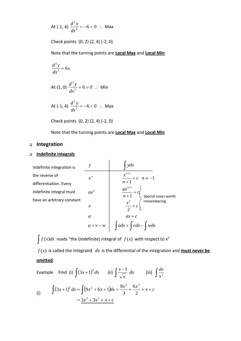
Integration

Indefinite integrals

wdxvdxudxwvu

caxa

cx

x

cn

axax

ncn

xx

ydxy

nn

nn

2

1

1 1

2

1

1

dxxf )( reads “the (indefinite) integral of )(xf with respect to x”

)(xf is called the integrand. dx is the differential of the integration and must never be

omitted.

Example Find (i) dxx2

13 (ii) dxx

x

1 (iii) 2x

dx

(i)

cxxx

cxxx

dxxxdxx

23

2322

33

2

6

3

916913

Indefinite integration is

the reverse of

differentiation. Every

indefinite integral must

have an arbitrary constant

added.

Special cases worth remembering

(ii)

cxxx

cxx

dxxxdxxx

xdx

x

x

2

1

1

32

21

23

2

1

2

3

2

1

2

1

(iii) Not a misprint! cx

dxxdxxx

dx

1.

1 12

22

cx

1

Definite integrals

If cxFdxxfI )()( , then the definite integral b

adxxf

)( is the difference in the

value of I when bx and ax .

i.e. )()()( aFbFdxxfb

a

no constant!

The limits of the definite integral are a (lower limit) and b (upper limit).

Note the use of square brackets. )()()( aFbFxFb

a

Example Evaluate

3

1 3

1dx

xx

9

40

2

1

2

1

18

1

2

9

2

1

2

22

1

3

1

2

2

3

1

223

1

33

1 3

x

x

xxdxxxdx

xx

Area on a graph as a definite integral

(i)

b

a

ydxA

0 a b x

y

A

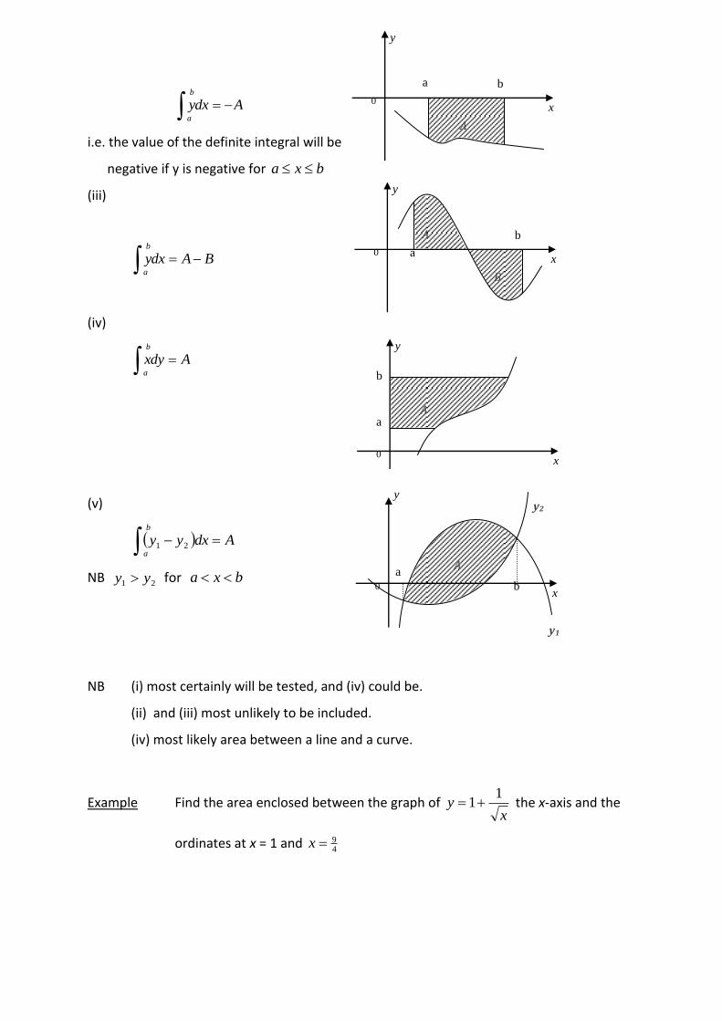
Aydxb

a

i.e. the value of the definite integral will be

negative if y is negative for bxa

(iii)

BAydxb

a

(iv)

Axdyb

a

(v)

Adxyyb

a

21

NB 21 yy for bxa

NB (i) most certainly will be tested, and (iv) could be.

(ii) and (iii) most unlikely to be included.

(iv) most likely area between a line and a curve.

Example Find the area enclosed between the graph of x

y1

1 the x-axis and the

ordinates at x = 1 and 49x

0

a b

x

y

A

0 a

b

x

y

A

B

0

a

b

x

y

A

0

a

b x

y

A

y2

y1

4

921

2

32

4

9

2

1 1

1

4

94

9

2

1

4

9

2

14

9

1

121

1

1

xxx

x

dxxdxx

A

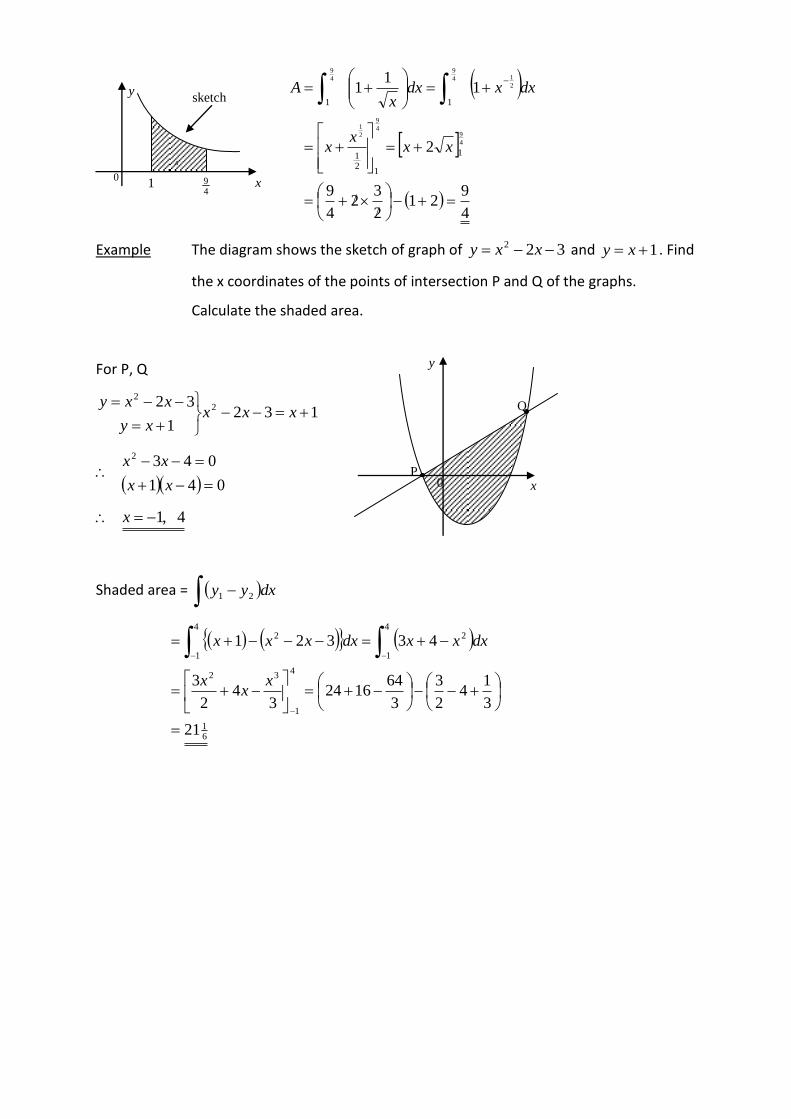
Example The diagram shows the sketch of graph of 322 xxy and 1 xy . Find

the x coordinates of the points of intersection P and Q of the graphs.

Calculate the shaded area.

For P, Q

1321

32 2

2

xxx

xy

xxy

041

0432

xx

xx

4 ,1x

Shaded area = dxyy 21

61

4

1

32

4

1

24

1

2

21

3

14

2

3

3

641624

34

2

3

43 321

x

xx

dxxxdxxxx

0 1

49

x

y

A

sketch

0 x

y

P

Q

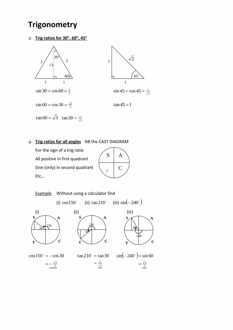
Trigonometry

Trig ratios for 30, 60, 45

2160cos30sin

2

145cos45sin

2

330cos60sin 145tan

360tan 3

130tan

Trig ratios for all angles NB the CAST DIAGRAM

For the sign of a trig ratio

All positive in first quadrant

Sine (only) in second quadrant

Etc…

Example Without using a calculator find

(i) 150cos (ii) 210tan (iii) 240sin

(i) (ii) (iii)

2

3

30cos150cos

3

1

30tan210tan

2

3

60sin240sin

60

30

3

1 1

2 2

45

1

1 2

S

T C

A

S A

C T

30

210

S A

C T

30 150

S A

C T

60

-240

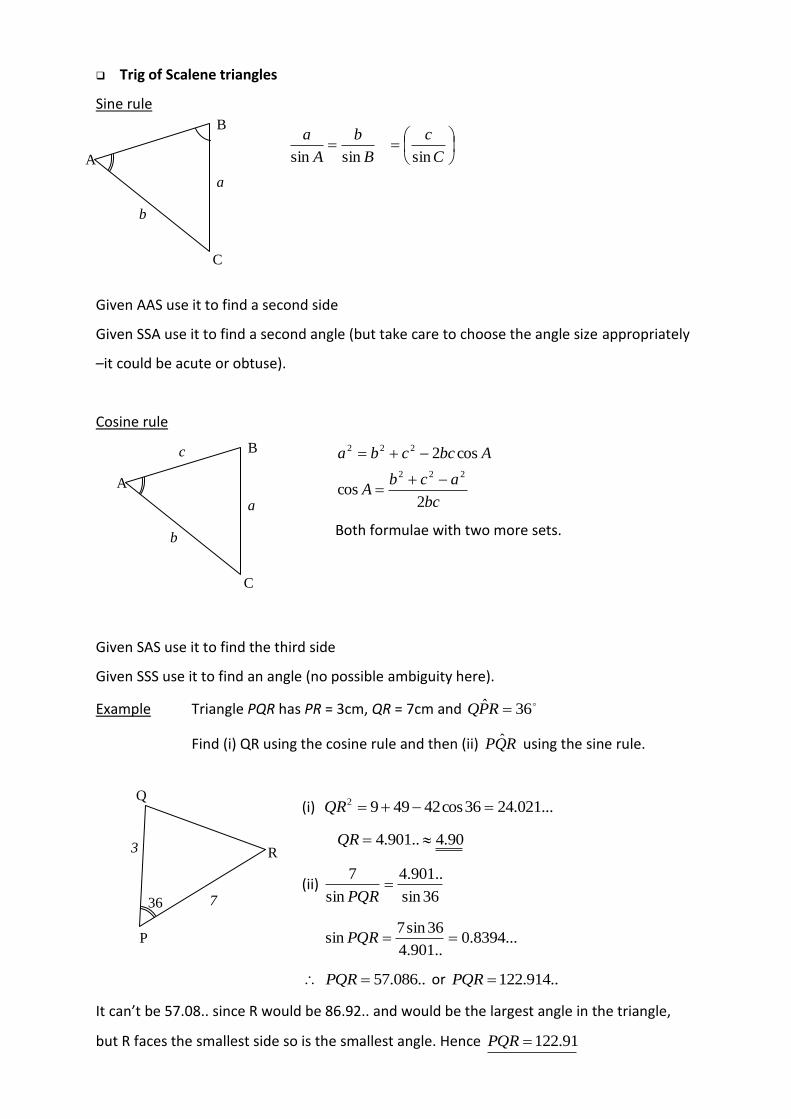
Trig of Scalene triangles

Sine rule

B

b

A

a

sinsin

C

c

sin

Given AAS use it to find a second side

Given SSA use it to find a second angle (but take care to choose the angle size appropriately

–it could be acute or obtuse).

Cosine rule

bc

acbA

Abccba

2cos

cos2

222

222

Both formulae with two more sets.

Given SAS use it to find the third side

Given SSS use it to find an angle (no possible ambiguity here).

Example Triangle PQR has PR = 3cm, QR = 7cm and 36ˆ RPQ

Find (i) QR using the cosine rule and then (ii) RQP ˆ using the sine rule.

(i) ...021.2436cos424992 QR

90.4..901.4 QR

(ii) 36sin

..901.4

sin

7

PQR

...8394.0..901.4

36sin7sin PQR

..086.57PQR or ..914.122PQR

It can’t be 57.08.. since R would be 86.92.. and would be the largest angle in the triangle,

but R faces the smallest side so is the smallest angle. Hence 91.122PQR

A

B

C

a

b

A

B

C

a

b

c

P

R

Q

7

3

36

Area “ Cabsin21 ” rule given SAS

Area of triangle = Cabsin21

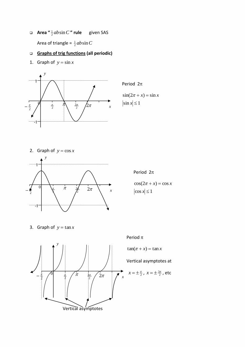
Graphs of trig functions (all periodic)

1. Graph of xy sin

Period 2

1sin

sin)2sin(

x

xx

2. Graph of xy cos

Period 2

1cos

cos)2cos(

x

xx

3. Graph of xy tan

Period

xx tan)tan(

Vertical asymptotes at

2x ,

23x , etc

Vertical asymptotes

2

0 2

2

3

2 x

y

0 2

1

-1

2

3

2 2

x

y

0 2

1

-1

2

3

2 2

x

y

Boundary values of trig ratios

Verify these from graphs

Two important trig identities

tan

cos

sin 1cossin 22

Example Given is obtuse and 178sin find the values of cos and

tan .

1cossin 22 22 sin1cos

289225

289641

1715cos

cos

sintan

158

1715

178

tan

NB Learn how to rearrange the identities

tancossin

tan

sincos

22 sin1cos 22 cos1sin

Trig equations Remember that from your calculator 1sin , 1cos and 1tan give the

principal value (p.v.)

Example Solve the equations

(i) 5.1tan for 3600

(ii) 5.02sin for 180180

(iii) sin1cos2 2 for 3600

(iv) cossinsin2 2 for 3600

(v) 2

380sin for 180180

S=1

C=0

S= -1

C=0

S=T=0

C=1

S=T=0

C= -1

T-

T

T

T-

S A

C T

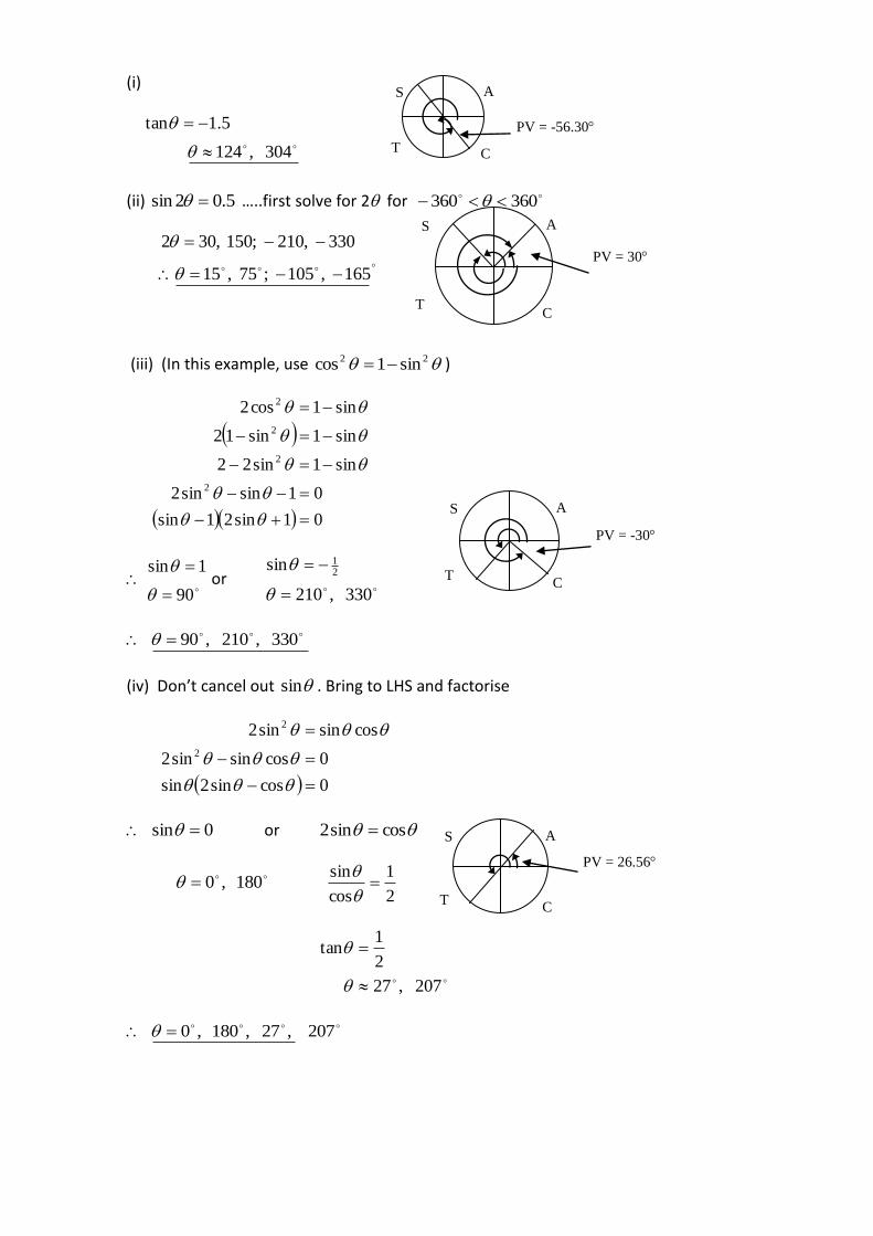
(i)

304 ,124

5.1tan

(ii) 5.02sin …..first solve for 2 for 360360

165 ,105 ;75 ,15

330 ,210 ;150 ,302

(iii) (In this example, use 22 sin1cos )

01sin21sin

01sinsin2

sin1sin22

sin1sin12

sin1cos2

2

2

2

2

90

1sin

or

330 ,210

sin21

330 ,210 ,90

(iv) Don’t cancel out sin . Bring to LHS and factorise

0cossin2sin

0cossinsin2

cossinsin2

2

2

0sin or cossin2

180 ,0 2

1

cos

sin

207 ,27

2

1tan

207 ,27 ,180 ,0

C T

S A

PV = 26.56

C T

S A

PV = -56.30

C T

S A

PV = 30

C T

S A

PV = -30

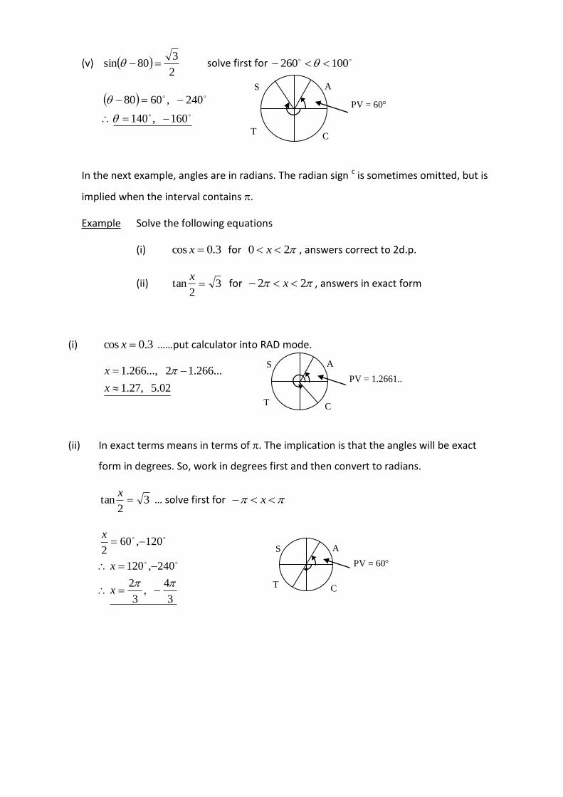
(v) 2

380sin solve first for 100260

160 ,140

240 ,6080

In the next example, angles are in radians. The radian sign c is sometimes omitted, but is

implied when the interval contains .

Example Solve the following equations

(i) 3.0cos x for 20 x , answers correct to 2d.p.

(ii) 32

tan x

for 22 x , answers in exact form

(i) 3.0cos x ……put calculator into RAD mode.

02.5 ,27.1

...266.12 ...,266.1

x

x

(ii) In exact terms means in terms of . The implication is that the angles will be exact

form in degrees. So, work in degrees first and then convert to radians.

32

tan x

… solve first for x

3

4 ,

3

2

240,120

120,602

x

x

x

C T

S A

PV = 60

C T

S A

PV = 1.2661..

C T

S A

PV = 60

Mechanics

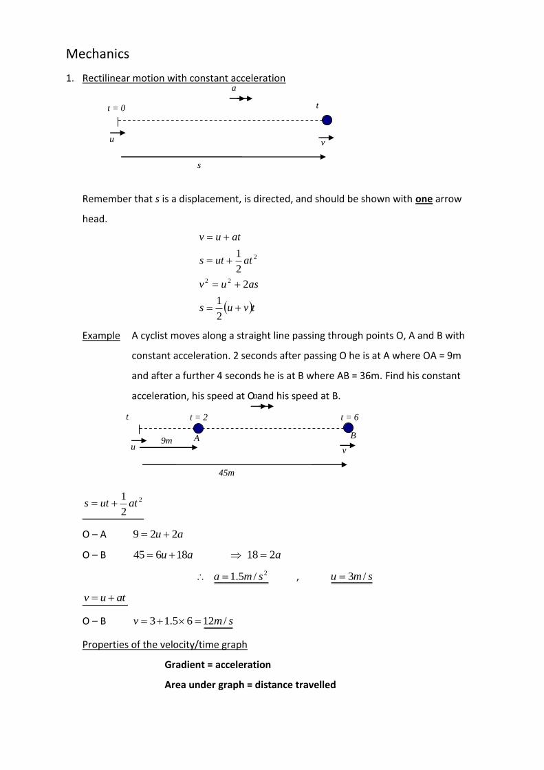
1. Rectilinear motion with constant acceleration

Remember that s is a displacement, is directed, and should be shown with one arrow

head.

tvus

asuv

atuts

atuv

2

1

2

2

1

22

2

Example A cyclist moves along a straight line passing through points O, A and B with

constant acceleration. 2 seconds after passing O he is at A where OA = 9m

and after a further 4 seconds he is at B where AB = 36m. Find his constant

acceleration, his speed at O and his speed at B.

2

2

1atuts

O – A au 229

O – B au 18645 a218

2/5.1 sma , smu /3

atuv

O – B smv /1265.13

Properties of the velocity/time graph

Gradient = acceleration

Area under graph = distance travelled

t = 0 t

v u

s

a

t = 6 t

v u

45m

a

A B

t = 2

9m

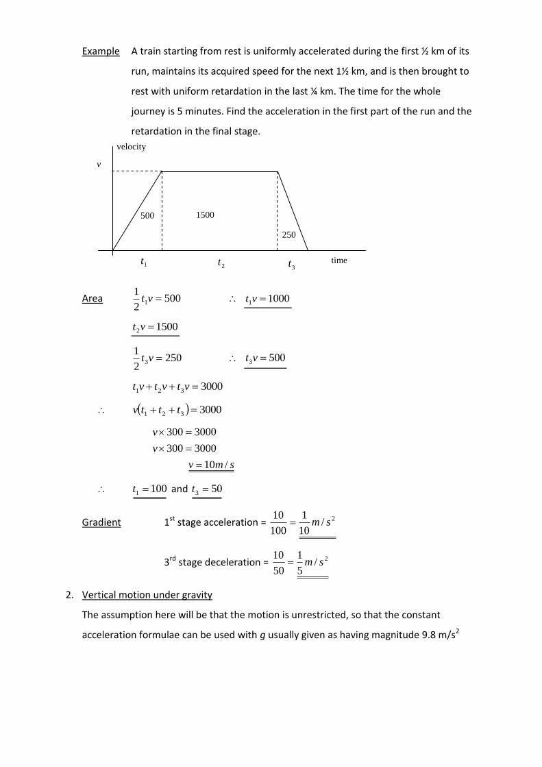
Example A train starting from rest is uniformly accelerated during the first ½ km of its

run, maintains its acquired speed for the next 1½ km, and is then brought to

rest with uniform retardation in the last ¼ km. The time for the whole

journey is 5 minutes. Find the acceleration in the first part of the run and the

retardation in the final stage.

Area 5002

11 vt 10001 vt

15002 vt

2502

13 vt 5003 vt

3000321 vtvtvt

3000321 tttv

smv

v

v

/10

3000300

3000300

1001 t and 503 t

Gradient 1st stage acceleration = 2/10

1

100

10sm

3rd stage deceleration = 2/5

1

50

10sm

2. Vertical motion under gravity

The assumption here will be that the motion is unrestricted, so that the constant

acceleration formulae can be used with g usually given as having magnitude 9.8 m/s2

1t

2t

3t

v

time

500 1500

250

velocity

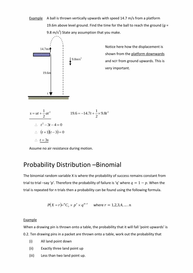
Example A ball is thrown vertically upwards with speed 14.7 m/s from a platform

19.6m above level ground. Find the time for the ball to reach the ground (g =

9.8 m/s2) State any assumption that you make.

Notice here how the displacement is

shown from the platform downwards

and NOT from ground upwards. This is

very important.

2

2

1atuts 28.9

2

17.146.19 tt

0432 tt

031 tt

st 3

Assume no air resistance during motion.

Probability Distribution –Binomial

The binomial random variable X is where the probability of success remains constant from

trial to trial –say ‘p’. Therefore the probability of failure is ‘q’ where 𝑞 = 1 − 𝑝. When the

trial is repeated for n trials then a probability can be found using the following formula.

rnrr

n qpCrXP where 𝑟 = 1,2,3,4,… .𝑛

Example

When a drawing pin is thrown onto a table, the probability that it will fall ‘point upwards’ is

0.2. Ten drawing pins in a packet are thrown onto a table, work out the probability that

(i) All land point down

(ii) Exactly three land point up

(iii) Less than two land point up.

9.8m/s2

14.7m/s

19.6m

t

𝑝 = 0.2, 𝑞 = 0.8

(i) P(all land point down) = 107.080.0 10

(ii) P(exactly three land point up) = 733

10 8.02.03 CXP

201.08.02.0120 73

(iii) P(less than two land point up) = 102 XPXPXP

375.0

8.02.010107.0 9