1

D-UNet: a dimension-fusion U shape network forchronic stroke lesion segmentation

Yongjin Zhou, Member, IEEE, Weijian Huang, Pei Dong, Yong Xia, and Shanshan Wang, Member, IEEE,

Abstract—Assessing the location and extent of lesions caused by chronic stroke is critical for medical diagnosis, surgical planning,and prognosis. In recent years, with the rapid development of 2D and 3D convolutional neural networks (CNN), the encoder-decoderstructure has shown great potential in the field of medical image segmentation. However, the 2D CNN ignores the 3D information ofmedical images, while the 3D CNN suffers from high computational resource demands. This paper proposes a new architecture calleddimension-fusion-UNet (D-UNet), which combines 2D and 3D convolution innovatively in the encoding stage. The proposedarchitecture achieves a better segmentation performance than 2D networks, while requiring significantly less computation time incomparison to 3D networks. Furthermore, to alleviate the data imbalance issue between positive and negative samples for the networktraining, we propose a new loss function called Enhance Mixing Loss (EML). This function adds a weighted focal coefficient andcombines two traditional loss functions. The proposed method has been tested on the ATLAS dataset and compared to threestate-of-the-art methods. The results demonstrate that the proposed method achieves the best quality performance in terms of DSC =0.5349±0.2763 and precision = 0.6331±0.295).

Index Terms—MRI, stroke segmentation, deep learning, dimensional fusion.

F

1 INTRODUCTION

S TROKE is the most common cerebrovascular diseaseand is one of the most common causes of death and

disability worldwide [1], [2]. It is a group of diseases causedby a sudden cerebrovascular rupture or cerebrovascularinfraction. The typical symptom of this disease is a focalneurological deficit, such as sudden seizures, language dis-orders, hemianopia, loss of feeling, etc. [3]. These symp-toms may develop into chronic diseases (such as dementia,hemiplegia, etc.), which can seriously affect the life qualityof patients; these diseases consume a large part of socialhealth care costs [4]. At the subacute/chronic stages, ef-fective rehabilitation can promote a long-term functionalrecovery. However, there have been few advances in large-scale neuroimaging-based stroke predictions at the subacuteand chronic stages. The most common research scan isa high-resolution T1-weighted structural MRI. Researchesusing these types of images at the subacture/chronic stageshave revealed promising biomarkers. These could poten-tially provide additional information, beyond behavioralassessments, to predict an individuals likelihood of recovery

• This work was supported by funding from the National Natural ScienceFoundation of China (61601450, 61871371, and 81830056), Science andTechnology Planning Project of Guangdong Province (2017B020227012)(Corresponding authors: Shanshan Wang)

• Y. Z and W. H are with the School of Shenzhen Univer-sity, Shenzhen 518060, China. E-mail: yjzhou@szu.edu.cn,2170249218@email.szu.edu.cn

• P. D is with School of Information Technologies, University of Sydney,NSW 2006, Australia.

• Y. X is with School of Computer Science, Northwestern PolytechnicalUniversity, Xian 710072, China.

• S. Wang is with the Paul C. Lauterbur Research Center for BiomedicalImaging, Shenzhen Institutes of Advanced Technology, Chinese Academyof Sciences, Shenzhen 518055, China. E-mail: ss.wang@siat.ac.cn, sophi-asswang@hotmail.com.

• Code will be available at: https://github.com/SZUHvern/D-UNet/tree/master.

for specific functions (e.g., motor, speech) and responseto treatments [5], [6]. Thus far, measures that include thesize, location, and overlap of the lesion with existing brainregions or structures, such as the corticospinal tract, havebeen successfully used as predictors of long-term strokerecovery and rehabilitation [7]. However, a key barrier tocorrectly analyzing these large-scale stroke neuroimagingdatasets to predict outcomes is the accurate segmentationof lesions. As manually-based annotations may no longerbe suitable for a wide range of data requirements, there is aneed for automatic segmentation tools for their analyses.

Strokes occur in different locations, with large differ-ences in shape and unclear boundaries as shown in Fig. 1. Apublic dataset, Anatomical Tracings of Lesions-After-Stroke(ATLAS), is utilized to illustrate this variability [7]. Firstly,the segmentation performance is reduced by motion arti-facts in the MRI images. Secondly, the position and shape ofthe lesions are significantly different owing to the existenceof multiple subtypes of strokes. The lesion volume can varyfrom hundreds to tens of thousands of cubic millimetersdepending on the severity of the disease, and the lesionarea can occur in the cerebrum, cerebellum, and other areasof the brain. Finally, the boundaries of some lesions arenot clear, and different clinicians may inconsistently labeldifferent lesion areas. Therefore, the accurate automatedsegmentation is a challenging problem.

To tackle these difficulties, researchers have made manyefforts, including intensity threshold processing, regiongrowth, and deformable models. However, these methodsrely on the hand-crafted feature extraction by experts; theyhave a limited feature representation and low generalizationperformance. In recent years, with the rapid development ofdeep learning, convolutional neural networks (CNN) haveproven to have great potential in the field of medical imageanalysis [7]–[17]. The study of CNN is mainly based on two-

arX

iv:1

908.

0510

4v1

[ee

ss.I

V]

14

Aug

201

9

2

Fig. 1. The MRI T1 sequence stroke image from the ATLAS dataset.The first column is the raw data, the second column is the gold standardfrom the hand-marked lesions by the doctor, and the third column is thecombination of the first two columns. Strokes occur in different locations,with large differences in shape and unclear boundaries.

dimensional (2D) and three-dimensional (3D) approaches:(1) In the 2D CNN approaches, the MRI volume data areconverted into several planar slices and independently pre-dict the lesion area of each slice. These ignore the spatialcharacteristics of the MRI data such that the predictionsare discontinuous. (2) In the 3D CNN, approaches, spatialinformation is extracted for inference. However, due to theircomputational and storage requirements, the 3D CNN havebeen largely avoided.

In order to solve the problem of accurately automatingthe image segmentation, we propose a novel network calledthe Dimension-fusion-UNet (D-UNet). In this new model,the 3D spatial information in the MRI data is effectivelyutilized under the 2D framework of the subject and haslow computing resource requirements. Our D-UNet has thefollowing two technical achievements:

Dimension fusion network: First, in order to extractthe information of consecutive slices from MRI data, wedesigned a novel downsampling block based on a UNetimprovement. This improvement performs 3D and 2D fea-ture extraction on a small number of consecutive slices inthe early stage of the network. Then, in a novel way, theirrespective feature maps are fused to achieve a small numberof parameters in the 2D network. Through the extractionof 3D features in the MRI data, D-UNet can achieve betterperformance than a pure 2D network.

Enhanced Mixing Loss: Second, in order to improvethe convergence speed of the network, we propose a new

loss function, called the Enhanced Mixing Loss, which notonly enhances the gradient propagation of the traditionalDice Loss, but also combines the advantages of the Dice lossand Focal loss functions. This new method converges fasterthan using the two traditional loss functions, and exhibits asmoother convergence curve. In summary, this work has thefollowing contributions: 1. We propose the D-UNet networkto effectively segment the lesion area in the MRI data. Thestructure is based on the 2D UNet improvement. A part ofthe 3D convolution is added to the downsampling moduleto extract the spatial information in the MRI volume data;the extracted features are fused with the 2D structures ina new method. 2. We propose a novel loss function, whichis expected to make the network converge in a faster andsmoother fashion. It would not only enhance the gradientpropagation in the traditional Dice loss, but also combinethe merits of Dice loss and Focal loss functions. 3. Theproposed method is tested on the ATLAS dataset and com-pared to three state-of-the-art, demonstrating the superiorperformance of the method.

2 RELATED WORKSWe summarize some of the work related to stroke seg-mentation, including hand-crafted feature based methodsand deep learning based methods. Among them, the deeplearning methods include 2D-based CNN, 3D-based CNN,and the traditional segmentation loss function.

Hand-crafted feature based methods: Researchers havebeen working on the automatic segmentation and predic-tion of brain disease areas and have achieved good results[18]. Kemmling et al. [19] use a multivariate computedtomography perfusion (CTP)-based model to calculate theprobability of voxelwise infarcts. Kuo et al. [20] propose touse the SVM classifier to learn texture feature vectors for thesegmentation of liver tumors. Chyzhyk et al. [21]proposeto construct an image data classifier from multimodal MRIdata for voxel-based lesion segmentations. Sivakumar et al.[22] use an adaptive neuro fuzzy inference system (ANFIS)classifier to detect and segment brain stroke areas auto-matically while using the heuristic histogram equalizationtechnique (HHET) to enhance the internal regions of thebrain image. These proposals in the literature are machinelearning models based on multiple linear regressions, rely-ing on the precise design of features by feature engineers.They achieve good performance on small sized data sets,but have limited generalization in larger data sets.

Deep learning based methods: Deep learning hasemerged in recent years, which address a key limitationin traditional machine learning methods, which requireengineers to artificially design features. Chen et al. [23]propose a 2D network framework consisting of an ensembleof a DeconvNets (EDD)-Net and a multi-scale convolutionallabel evaluation net (MUSCLE Net); this ensemble achievesthe best performance on a large clinical dataset. Cui et al.[24] propose a network of cascaded structures for process-ing nasopharyngeal carcinoma cases in MRI images. Theauthors firstly segment the tumors and then classify thesegmentation results to obtain four subregions of nasopha-ryngeal carcinoma. These deep learning methods convertthe MRI data to 2D slices and apply 2D segmentation CNN

3

for each slice. The 3D results are generated by connecting the2D segmentation results. However, due to the limitations ofthe slices 2D characteristics, the important 3D context infor-mation in the volume data is neglected, thus the predictionmay lose continuity.

3D CNN has proven to have great potential in theanalysis of 3D MRI data. Kamnitsas et al. [25] propose atwo-path 3D CNN structure and uses a 3D fully connectedconditional random field for post processing, which ranksfirst in the challenge of chronic stroke lesion segmentation(ISLES 2015). Zhang et al. [10] propose 3D FC-DenseNet,which can make the network deeper by using the improveddense net tight connection structure to enhance the backpropagation of image information and gradients. Feng etal. [26] extract features from both the temporal and thespatial dimensions by using 3D convolution operations,which capture the dynamic information in multiple adjacentframes. However, they usually require more parameters andmight sometimes over-fit on small training data sets [27],[28]. In addition, 2D-based and 3D-based cascade methodshave emerged. For example, Li et al. [29] propose a hybriddensely connected UNet (H-DenseUNet), which first per-forms a 2D-based dense-UNet segmentation, and then usesa 3D-based CNN to correct the spatial continuity of the liverand the tumor.

The binary cross-entropy loss function [30] is commonlyused in deep learning based segmentation tasks. This func-tion calculates the gradient by characterizing the differencein the probability distribution of each pixel in the predictedsample and the real sample. Tsung-Yi Lin et al. [31] adda modulating factor to deal with the serious imbalancebetween the number of foreground and background pixels.Another common loss function is Dice’s coefficient loss [32].This function directly calculates the gradient by the diceoverlap coefficient of the predicted sample and the reallabel; it can also alleviate to some extent the segmentationproblem resulting from the pixel imbalance between theforeground and the background.

3 METHODS

In this section, we introduce our approach including theproposed D-UNet framework, enhanced mixing loss, andthe implementation details. In Section 3.1, we illustrate theproposed D-UNet framework, in Section 3.2, we introducethe enhanced mixing loss algorithm, and finally in Section3.3, we present some implementation details.

3.1 D-UNet for extracting three-dimensional informa-tion

The basic structure of the network consists of an improvedUNet [33]. This symmetrical encoder-decoder structurecombines high-level semantics with low-level fine-grainedsurface information; it has achieved good effects on medicalimages. The encoding phase of the D-UNet consists of twodimensions. As shown in Fig. 2(a), both the 2D and 3Dconvolutions perform the downsampling operation in theirrespective dimensions; the results are combined through thedimension transform block which denote as a red cube. Thisfusion enables subsequent 2D networks to be integrated into

the 3D information, refines the edges of the target area,and facilitates the ability of the network to identify smalllesion areas. Meanwhile, since the 3D information is wellextracted in the early stage of the network, and the trainableparameters of the network are extremely increased as thenetwork deepens, the dimension transform block is onlyadded in the early coding stage.

Specifically, consider Fig. 2(b), where H×W denotes thefeature dimensions of height and width, D represents thedepth in the volume feature, and C represents the channelof the feature map. The dimension transform block consistsof 3D dimensionality reduction, channel excitation [34], anddimensional fusion. The squeeze-and-excite (SE) block hasbeen proposed in recent years, where r denotes the reduc-tion ratio, a hyperparameter which allows us to vary thecapacity and computational cost of the SE block [34]. Thisblock activates the connection between different channelsby weighting the feature channels. We apply this structurein the dimension fusion block in order to enhance the fusioneffect of 3D features and 2D features.

In each dimension transform block, we first reduce thedimensions of the 3D branch feature map and then add withthe 2D branch after SE weighted respectively. Specifically,let I3d and I2d denote the feature maps from 3D and 2Dnetwork respectively, which act as the input of dimensiontransform block, n denotes the batch size, h×w× d denotesthe maps height, width, depth and last dimension c denotesthe maps channel. We first convert I3d∈Rn×h×w×d×c toI∗3d∈Rn×h×w×d×1 by using a 3D 1×1×1 convolution whichfilter number is set to 1, then we squeeze the dimensionalityof I∗3d from n × h × w × d × 1 to n × h × w × d. In orderto keep the channel number consistent with the 2D branchfor later integration, we also convert I∗3d∈Rn×h×w×d toI∗3d∈Rn×h×w×c by using a 2D 3×3 convolution that filternumber is set to c. Let I

′3d denote the I3d after dimensional-

ity reduction:

I′

3d = fr(I3d), I′

3d ∈ Rn×h×w×c (1)

where fr indicates the dimensionality reduction opera-tion, thus we convert the size of 3D feature map fromI3d∈Rn×h×w×d×c to I

′

3d ∈ Rn×h×w×c. In order to enhancethe feature expression ability of the two dimensions beforefusion, we use an SE block to weight the 3D and 2D featuremap channels, and add their channel weighted outputs:

T = fSE(I′

3d) + fSE(I2d), T ∈ Rn×h×w×c (2)

The 3D and 2D features are fused in this step, where fSEdenotes the SE weighted block proposed in [34]. T denotesthe feature map fusion which results in the dimensionfusion block. More detailed parameter settings for the entirenetwork are shown in Table 1.

3.2 Enhanced Mixing Loss Function

In 3D medical data, especially MRI stroke images as shownin Fig. 1, the volume occupied by the stroke is often verysmall throughout the scan interval. An extremely large num-ber of background regions may dominate the loss functionduring training, which leads to the learning process easilyfalling into a local optimal solution. Therefore, we propose

4

Up-

Sampling

2D

Max-

Pooling

2d

Concatenate

BN

Conv2d

Conv2d

BN

Conv3d

BN

Conv3d

BN

Max-

pooling

3d

192×192×1

(a) D-Unet architecture

96×96×2

×32

96×96×2

×64

96×

96×

2

×6

4

96×96

×64

48×48×1

×64

192×192×4

×32

48×

48×

1

×1

28

48×48

×128

(b) Dimension Transform Block

HxWxC

Global

poolingFC ReLu FC Sigmoid

Mul

1×1×C 1×1×C/r 1×1×C/r 1×1×C

Squeeze-and-Excitation Block

H×W×C

Global

poolingFC ReLu FC Sigmoid

Mul

1×1×C 1×1×C/r 1×1×C/r 1×1×C

Conv3d

(1×1×1)Squeeze Conv2d

(3×3)

H×W×D×C H×W×D×1 H×W×D H×W×C

H×W×C

Add

H×W×C

Dimension

Transform

Block

Fig. 2. The entire D-UNet architecture is shown in (a). This network improves 2D UNet, which combines 3D convolution in the downsampling phaseand uses a dimension transform block to combine them. (b) Introduces the details of the dimension transform block, which has two branches for itsinput from 2D and 3D networks. First, the feature channel of the 3D network output (blue arrow) is compressed to 1 by using a 1x1x1 convolution.The compressed result is then squeezed in a spatial dimension and passed to a 2D 3x3 convolution. This makes the output consistent with the 2Dnetwork (gray arrow). Finally, each of the channels is weighted by the SE-block and then added together.

a new loss function, which refers to the method addressingthe foreground-background voxel imbalance in [31], andcombines two traditional loss functions in a concise manner[32].

3.2.1 Focal LossFocal loss (FL) is an improvement of the binary crossentropy loss (BCE), by adding a modulating factor. Thisreduces the loss contribution from easy samples and extendsthe range in low loss. We introduce the formula of focal lossfrom the binary cross entropy (BCE):

FL(p, g) =

{−∑Nf

i=1 α(1− p)γ log(p), if g = 1

−∑Nb

i=1(1− α)pγ log(1− p), otherwise(3)

where g ∈ 0, 1 represents the ground truth based onthe pixel level; p ∈ [0, 1] represents the model predictionprobability value, in which 0 denotes the background and1 is the foreground; Nf and Nb represent the numbers ofpixels of class 0 and class 1, respectively; α ∈ (0, 1] and

γ ∈ [0, 5] are the modulation factors, which can be flexiblyadjusted according to the situation.

3.2.2 Dice Coefficient LossThe dice coefficient loss (DL) mitigates the imbalance prob-lem of background and foreground pixels by modifying thesegmentation evaluation index DSC between the predictionsamples and the ground truth annotation, showing betterperformance in the segmentation task:

DL(p, g) = 1− 2∑Ni=1 pigi + δ∑N

i=1 p2i +

∑Ni=1 g

2i + δ

(4)

where δ ∈ [0, 1] is a tunable parameter to prevent a divide-by-zero error and let the negative samples also have agradient propagation.

3.2.3 Proposed Enhanced Mixing LossBased on the above two kinds of loss, we propose theenhanced mixing loss (EML) to increase the convergence

5

TABLE 1Architecture of the proposed D-UNet. Feature size denotes the size of the manipulated feature map while the last dimension indicates the channel

number. Up-sampling [*] indicates that the corresponding layer number is concatenated before up sampling and N∗ indicates the number offeatures of the corresponding layer number, for example, Up-sampling block 1 being connected to Convolution block 4, N is set to 256, up

sampling block 2 being connected to dimension fusion block 3, N is set to 128, and so on.

Feature size Two-dimensional operation Feature size Three-dimensional operation

Input 192×192×4 - 192×192×4×1 -

Convolution block 1 192×192×32 2×(3×3 Conv+ Bn) 192×192×4×3 2×(3×3×3 Conv+ Bn)

Pooling 96×96×32 2×2 max pooling 96×96×2×32 2×2×2 max pooling

Convolution block 2 96×96×64 2×(3×3 Conv+ Bn) 96×96×2×64 2×(3×3×3 Conv+ Bn)

Dimension fusion block 2 96×96×64 - - -

Pooling 48×48×64 2×2 max pooling 48×48×1×64 2×2×2 max pooling

Convolution block 3 48×48×128 2×(3×3 Conv+ Bn) 48×48×1×128 2×(3×3×3 Conv+ Bn)

Dimension fusion block 3 48×48×128 - - -

Pooling 24×24×128 2×2 max pooling - -

Convolution block 4 24×24×256 2×(3×3 Conv+ Bn) - -

Dropout 24×24×256 - - -

Pooling 12×12×256 2×2 max pooling - -

Convolution block 5 12×12×512 2×(3×3 Conv+ Bn) - -

Dropout 12×12×512 - - -

Up-sampling block 1-4 192×192×32 2×2 Up-sampling[*] - -2×(3×3 Conv+ Bn)

Convolution 192×192×1 1×1 Conv - -

speed. First, Log value was used in DL and we invertthe value for keeping the value positive, thus enhancingthe gradient obtained for each iteration. Then, in order toexplore whether the two losses have mutually reinforcingrelationships, we also add the focal loss. However, sincethe focal loss is based on the sum of all voxel proba-bilities, it is numerically much larger than the dice loss(DL(p, g) ∈ [0, 1]), which plays a leading role in gradientpropagation. We hope that the newly added FL and log(DL)contribute equally to EML, so a balance factor of 1/N isadded to FL to obtain a FL based voxel average. The formulafor EML is as follows:

EML(p, g) =1

NFL(p, g)− log(DL(p, g)) (5)

3.3 Implementation details

In the data preprocessing, transverse section images havebeen selected for this experiment. Within each image, asquare area is selected with the diagonal coordinates (10,40) and (190, 220). This selected area eliminates irrelevantinformation and enlarges the proportion of stroke lesionsin the entire image. Next, the cropped images are resized192 × 192 using a bilinear interpolation. Finally, each sliceof the processed image is integrated, with a spatial arrange-ment of two upper slices and one lower slice, forming amatrix of size 192 × 192 × 4. In the downsampling phase,modifications to reduce the total number of parameters fromUNet are made. Specifically, the number of filters in the firstconvolution in the 2D-based and 3D-based streams is setto 32. After each pooling layer, the number of convolutionfilters is doubled, and finally the number of convolutionsin the 2D stream is set to 512. The kernal initialization foreach convolution is set using the Hes method [35]. A batchnormalization is conducted after each layer of convolutionto improve the stability of the training. The parameter r inthe dimension transform block is set to 16. α, γ, δ in the loss

function is set to 1.1, 0.48, 1 respectly to fit our randomlyselected dataset. With the SGD optimizer, the learning rate isset to 1e-6. Additional parameter settings are consistent with[36]. We have also employed data augmentation methodsto improve the robustness of the model, including settingthe input mean to zero translation, scaling, and horizontalflipping. These methods are applied to all of our compar-ative experiments to ensure fairness. We have trained themodels on three 1080TI GPUs. All of the models are trainedusing the first 150 epochs before validating, to optimize theperformance of each architecture without any fine tuning.

4 EXPERIMENTAL RESULTS AND DISCUS-SIONSWe compare our proposed method to the 2D and 3D convo-lutional UNet. In this section, we also show the superiorityof the proposed loss and discuss the results of the proposeddimension-transform block at different stages. Datasets andquantitative indicators: We have used the Anatomical Trac-ings of Lesions-After-Stroke (ATLAS) dataset [7] as ourtraining and validation sets. The dataset contains 229 casesof chronic stroke with MRI T1 sequence scans, in whichthe size of each case is 233×197×189 while the physicalsize is 0.9×0.9×3.0mm3; the scans delineate different lesiongrade staging. We have randomly selected 183 cases (ac-counting for the overall 0.8 ratio) as the training set, and theremaining cases as validation sets. We report the model’sperformance in the Dice Similarity Coefficient (DSC), pre-cision, and recall. DSC is an important indicator to assessthe overall difference between our estimates and the groundtruths. Recall usually reflects the extent of recall in the lesionarea, which is an important reference in clinical practice.We perform threshold processing on all of the predictionresults. When the probability that the pixel is predicted tobe foreground is less than 0.5, we set it to zero, otherwiseit is set to one. In addition, precision evaluates the quality

6

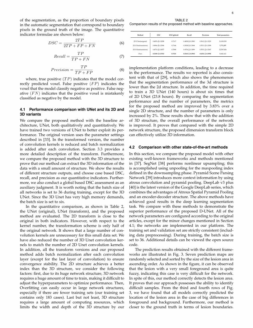
of the segmentation, as the proportion of boundary pixelsin the automatic segmentation that correspond to boundarypixels in the ground truth of the image. The quantitativeindicator formulae are shown below:

DSC =2TP

2TP + FP + FN(6)

Recall =TP

TP + FN(7)

Precision =TP

TP + FP(8)

where, true positive (TP ) indicates that the model cor-rectly predicted voxel. False positive (FP ) indicates thevoxel that the model classify negative as positive. False neg-ative (FN) indicates that the positive voxel is mistakenlyclassified as negative by the model.

4.1 Performance comparison with UNet and its 2D and3D variantsWe compare the proposed method with the baseline ar-chitecture, UNet, both qualitatively and quantitatively. Wehave trained two versions of UNet to better exploit its per-formance. The original version uses the parameter settingsdescribed in [33]. In the transformed version, the numberof convolution kernels is reduced and batch normalizationis added after each convolution. Section 3.3 provides amore detailed description of the transform. Furthermore,we compare the proposed method with the 3D structure toprove that our method can extract the 3D information of thedata with a small amount of structure. We show the resultsof different structure outputs, and choose case based DSC,recall, and precision as our quantitative indicators. Further-more, we also conduct a global based DSC assessment as anauxiliary judgment. It is worth noting that the batch size ofall networks is set to 36 during training, except for the 3DUNet. Since the 3D Unet has very high memory demands,the batch size is set to six.

In the quantitative comparison, as shown in Table 2,the UNet (original), UNet (transform), and the proposedmethod are evaluated. The 2D transform is close to theoriginal in both indicators. However, with respect to thekernel number, the transformation scheme is only half ofthe original network. It shows that a large number of con-volution kernels are unnecessary for this small data set. Wehave also reduced the number of 3D Unet convolution ker-nels to match the number of 2D Unet convolution kernels.In addition, all the transform versions and our proposedmethod adds batch normalization after each convolutionlayer (except for the last layer of convolution) to ensureconvergence stability. The 2D structure achieves a betterindex than the 3D structure, we consider the followingfactors: first, due to its huge network structure, 3D networkrequires a huge amount of time to train, making it difficult toadjust the hyperparameters to optimize performance. Then,Overfitting can easily occur in large network structures,especially if there are fewer training sets (our training setcontains only 183 cases). Last but not least, 3D structurerequires a large amount of computing resources, whichlimits the width and depth of the 3D structure by our

TABLE 2Comparison results of the proposed method with baseline approaches.

Method DSC DSC(global) Recall Precision Total parameters

2D UNet(original) 0.4874±0.2858 0.7117 0.4838±0.2983 0.5612±0.3229 31,030,593

2D UNet(transform) 0.4966±0.2906 0.7146 0.5038±0.3044 0.5511±0.3298 7,771,297

3D UNet(transform) 0.4710±0.2877 0.7098 0.4736±0.3099 0.5531±0.3247 22,597,826

Ours 0.5349±0.2763 0.7231 0.5243±0.2910 0.6331±0.2958 8,640,163

implementation platform conditions, leading to a decreasein the performance. The results we reported is also consis-tent with that of [29], which also shows the phenomenonthat the segmentation performance of the 3d structure islower than the 2d structure. In addition, the time requiredto train a 3D UNet (140 hours) is about six times thatof 2D UNet (23.8 hours). By comparing the segmentationperformance and the number of parameters, the metricsfor the proposed method are improved by 3.83% over asingle 2D structure, and the number of parameters is onlyincreased by 2%. These results show that with the additionof 3D structure, the overall performance of the networkis improved. It proves that compared with the simple 2Dnetwork structure, the proposed dimension transform blockcan effectively utilize 3D information.

4.2 Comparison with other state-of-the-art methods

In this section, we compare the proposed model with otherexisting well-known frameworks and methods mentionedin [37]. SegNet [38] performs nonlinear upsampling; thisis accomplished using unpooling for the maxpooling indexdefined in the downsampling phase. Pyramid Scene ParsingNetwork [39] introduces more context information by usingatrous convolution and pyramid pooling. DeepLab v3 plus[40] is the latest version of the Google DeepLab series, whichcombines the advantages of Atrous Spatial Pyramid Poolingand an encoder-decoder structure. The above methods haveachieved good results in the deep learning segmentationtask. We compare with these methods to demonstrate thesuperior performance of the proposed D-UNet. All of thenetwork parameters are configured according to the originalarticles, except for the minor changes mentioned in Section4.1; the networks are implemented in our platform. Thetraining set and validation set are strictly consistent (includ-ing data preprocessing). During training, the batch size isset to 36. Additional details can be viewed the open sourcecode.

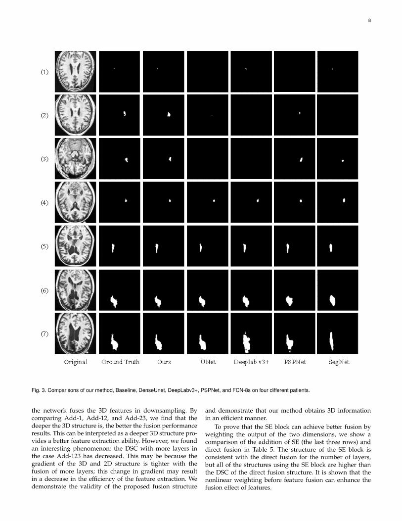
The prediction results obtained with the different frame-works are illustrated in Fig. 3. Seven prediction maps arerandomly selected and sorted by the size of the lesion area inascending order. As shown in the figure, it can be observedthat the lesion with a very small foreground area is quitefuzzy, indicating this case is very difficult for the network.In spite of this, our method correctly detects the lesion area.It proves that our approach possesses the ability to identifydifficult samples. From the third and fourth rows of Fig.3, we have found that all models correctly predicted thelocation of the lesion area in the case of big differences inforeground and background. Furthermore, our method iscloser to the ground truth in terms of lesion boundaries.

7

Observing the last two rows, we have found that the pro-posed method still maintains a good, feature expressionability when the boundary is very blurry. This is because wecombine the 3D features and the spatial dimensions to moreeffectively express the characteristics of the edge blurredlesions. In order to show the distribution of the results andprove the stability of the proposed method, we draw a boxplot based on the DSC score for each case. These resultsare shown in Fig. 4. The lower edge of all methods is zerobecause the ATLAS data set has a very large number ofsmall lesion areas (e.g., the first to third rows of Fig. 3),which easily cause the model to fail to recognize the lesions.The upper edge and median line for the proposed methodare the best in comparison with other highly recognizedmethods, which means it not only achieves the highestsegmentation performance on a single case, but also yieldsbetter median scores for all cases.

To quantitatively illustrate the superiority of ourmethod, we compare the results of these algorithms andsummarize them in Table 3, where DSC, recall, and precisionare based on the mean ± standard deviation of each case,and DSC (global) represents the metric based on the voxelcalculation. Hu et al. use the ATLAS dataset, and select somespecific cases as training/validation sets to summarize sometraditional segmentation methods. We compare several deeplearning segmentation frameworks with the methods men-tioned in [37]. The top half of the table shows the imple-mentation in [37], and the bottom half is implemented onour platform. It can be seen from the table that the deeplearning based methods achieve better performance than thetraditional algorithms. With respect to the DSC scores, theproposed method ranked first with a score of 0.7231. This is0.30 higher than the Clusterize method in DSC (the lowest),and 0.0383 higher than the UNet method (second best). Ourmethod is superior in terms of the segmentation perfor-mance for each case. DSC (global) can reflect a voxel-basedoverall DSC score more intuitively. With respect to recalland precision, the performance of the traditional algorithmClusterize is the highest in recall, but its precision score isthe lowest, which indicates that this algorithm identifiesmany non-lesional areas as lesions, thus causing a highrecall. The proposed method ranked third in the recall scoreof 0.5243, and the highest in the precision score of 0.6631,which indicates that the identified regions are basically thecorrect lesion areas.

4.3 Loss validity

In order to compare the effectiveness of the proposed loss,we trained on the proposed model and compared severalcommon losses in the segmentation task. As illustrated inFig. 5, the results show several DSC rising graphs on thetraining sets as the number of training iterations increases.Comparing the scores of the losses in the training set, in theearly stage of training (about 30 epoch) shown on Fig. 5, thedice coefficient loss converges faster than the focal loss, butis subsequently exceeded by the focal loss. In each period,our method converges faster than other methods.

We also performed a quantitative analysis of the threelosses, as shown in Table 4. It is worth noting that ourgoal is to make the proposed model converge faster. This

TABLE 3The quantitative comparison of different methods. Among them, DSC,

Recall, and Precision are based on the mean ± standard deviationcalculated in each case, and DSC (global) represents the DSC based

on the voxel calculation.

Method DSC DSC(global) Recall Precision

Clusterize 0.23±0.19 - 0.79±0.23 0.16±0.15

ALI 0.36±0.25 - 0.55±0.31 0.31±0.25

Lesion gnb 0.36±0.23 - 0.69±0.29 0.30±0.20

LINDA 0.45±0.31 - 0.52±0.34 0.50±0.34

SegNet 0.3292±0.2514 0.5993 03318±0.2654 0.3846±0.2883

PSP 0.4462±0.2633 0.6729 0.4704±0.2780 0.4998±0.2913

Deeplab v3 plus 0.4529±0.2921 0.7104 0.4456±0.3032 0.5627±0.3249

UNet 0.4966±0.2906 0.7146 0.5038±0.3044 0.5511±0.3298

Ours 0.5349±0.2763 0.7231 0.5243±0.2910 0.6331±0.2958

TABLE 4Quantitative analysis of the three loss functions.

Method DSC(global) Recall Precision

FL 0.6805 0.4339±0.2625 0.6225±0.3667DL 0.7346 0.53±0.2908 0.6143±0.3324

EML 0.7231 0.5243±0.2910 0.6331±0.2958

statistical score is only used as a secondary reference. SinceDL directly uses 1 - DSC as punished, it has an advantageto achieve the highest DSC score. Therefore, despite theproposed EML is slightly lower than DL in DSC (0.0115lower) and Recall (0.057±0.002 lower), we consider that itis within an acceptable range. On the other hand, EMLachieves the highest precision whereas DL presents thelowest, which indicates that EML can effectively reduce thefalse positive results (This phenomenon is also consistentwith FL). Therefore, EML is competitive in segmentationperformance compared to DL and FL.

4.4 Comparison of dimension fusion blocks betweendifferent layers

We also compare the results of the dimension transformblock used in different ways (Add, SE) and in differentdownsampling layers. The DSC is used as the main eval-uation index of model performance, and the number oftheir parameters is enumerated. The 3D framework usedin the experiment, as shown in Fig. 2, has only two poolinglayers for the dimension transform block within three layers.The ’add’ in Table 5 represents the use of the final fusionoperation of the dimension fusion block, (i.e., the Add blockin Fig. 2), and the ’SE’ indicates the use of the SE block thefigure [34]. The last column of the name in the architectureindicates which layer is used in the conversion structure. Forexample, ’Add-23’ means the corresponding 3D structurefusion before the second and third maxpooling in the 2Dstructure.

In order to prove the validity of dimensional transfor-mation on 2D networks, we compare the performance ofUNet (division) and different structures using the dimen-sion fusion block in different layers. All of the results withusing the dimensional fusion are better than UNet withoutusing the dimension fusion block. We suspect this is because

8

Fig. 3. Comparisons of our method, Baseline, DenseUnet, DeepLabv3+, PSPNet, and FCN-8s on four different patients.

the network fuses the 3D features in downsampling. Bycomparing Add-1, Add-12, and Add-23, we find that thedeeper the 3D structure is, the better the fusion performanceresults. This can be interpreted as a deeper 3D structure pro-vides a better feature extraction ability. However, we foundan interesting phenomenon: the DSC with more layers inthe case Add-123 has decreased. This may be because thegradient of the 3D and 2D structure is tighter with thefusion of more layers; this change in gradient may resultin a decrease in the efficiency of the feature extraction. Wedemonstrate the validity of the proposed fusion structure

and demonstrate that our method obtains 3D informationin an efficient manner.

To prove that the SE block can achieve better fusion byweighting the output of the two dimensions, we show acomparison of the addition of SE (the last three rows) anddirect fusion in Table 5. The structure of the SE block isconsistent with the direct fusion for the number of layers,but all of the structures using the SE block are higher thanthe DSC of the direct fusion structure. It is shown that thenonlinear weighting before feature fusion can enhance thefusion effect of features.

9

Fig. 4. Box plots of DSC score results for different methods.

Fig. 5. The DSC score curve of the training set during the trainingprocess.

TABLE 5Comparison results of the proposed method with baseline approaches.

Architecture DSC Total parameters

2D UNet(transform) 0.4966±0.2906 7,771,297Add-1 0.5102±0.2932 7,802,210

Add-12 0.5216±0.2776 7,970,019Add-23 0.5248±0.2770 8,635,043Add-123 0.5110±0.2762 8,636,260

SEAdd-12 0.5235±0.2851 7,971,299SEAdd-23 0.5349±0.2763 8,640,163SEAdd-123 0.5186±0.2865 8,647,012

5 CONCLUSION

Automated stroke segmentation plays an important rolein clinical diagnosis and prognosis. It is of great value toquickly and accurately identify areas of the lesions and helpphysicians make surgical plans without high computingresource demands. In this paper, we propose an end-to-endtraining method for the automatic stroke segmentation, inwhich 3D context information can be effectively utilized,with low hardware requirements. Meanwhile, we proposea new loss function for faster and smoother convergence.The proposed method has been compared with three state-of-the-art methods; it achieves the best performance ontwo quality metrics (DSC = 0.5349±0.2763, Precision =0.6331±0.2958). In future work, we hope to increase thepunishment for extremely difficult samples inspired from[41], which may further enhance the performance of theproposed EML. We plan to validate our method on a largerclinical dataset to verify the generalization of the methodin the current 3D structure, further study the possibilityof dimension fusion block combinations, and extend ourmodel to different applications, for example, calculatingoverlap of the lesion with existing brain regions or struc-tures, for used as predictors of long-term stroke recoveryand rehabilitation.

ACKNOWLEDGMENTS

This research was partly supported by the NationalNatural Science Foundation of China (61601450,61871371, 81830056), Science and Technology PlanningProject of Guangdong Province (2017B020227012,2018B010109009), the Basic Research Program of Shenzhen(JCYJ20180507182400762), Youth Innovation PromotionAssociation Program of Chinese Academy of Sciences(2019351).

REFERENCES

[1] Ferlay J, Shin H R, Bray F, et al. Estimates of worldwide burdenof cancer in 2008: GLOBOCAN 2008[J]. International journal ofcancer, 2010, 127(12): 2893-2917.

[2] Lu R, Marziliano P, Thng C H. Liver tumor volume estimation bysemi-automatic segmentation method[C]. 2005 IEEE Engineeringin Medicine and Biology 27th Annual Conference. IEEE, 2006:3296-3299.

[3] Van der Worp H B, van Gijn J. Acute ischemic stroke[J]. NewEngland Journal of Medicine, 2007, 357(6): 572-579.

[4] Saka , McGuire A, Wolfe C. Cost of stroke in the United King-dom[J]. Age and ageing, 2009, 38(1): 27-32.

[5] Neumann A B, Jonsdottir K Y, Mouridsen K, et al. Interrateragreement for final infarct MRI lesion delineation[J]. Stroke, 2009,40(12): 3768-3771.

[6] Martel A L, Allder S J, Delay G S, et al. Measurement of in-farct volume in stroke patients using adaptive segmentation ofdiffusion weighted MR images[C]. International Conference onMedical Image Computing and Computer-Assisted Intervention.Springer, Berlin, Heidelberg, 1999: 22-31.

[7] Liew S L, Anglin J M, Banks N W, et al. A large, open sourcedataset of stroke anatomical brain images and manual lesionsegmentations[J]. Scientific data, 2018, 5: 180011.

[8] Joshi S, Gore S. Ishemic Stroke Lesion Segmentation by AnalyzingMRI Images Using Dilated and Transposed Convolutions in Con-volutional Neural Networks[C]. 2018 Fourth International Con-ference on Computing Communication Control and Automation(ICCUBEA). IEEE, 2018: 1-5.

[9] Liu Z, Cao C, Ding S, et al. Towards clinical diagnosis: Automatedstroke lesion segmentation on multi-spectral MR image using con-volutional neural network[J]. IEEE Access, 2018, 6: 57006-57016.

10

[10] Zhang R, Zhao L, Lou W, et al. Automatic segmentation ofacute ischemic stroke from DWI using 3-D fully convolutionalDenseNets[J]. IEEE transactions on medical imaging, 2018, 37(9):2149-2160.

[11] Pereira D R, Reboucas Filho P P, de Rosa G H, et al. Strokelesion detection using convolutional neural networks[C]. 2018International joint conference on neural networks (IJCNN). IEEE,2018: 1-6.

[12] Charmchi S, Punithakumar K, Boulanger P. Optimizing U-Net to Segment Left Ventricle from Magnetic Resonance Imag-ing[C]. 2018 IEEE International Conference on Bioinformatics andBiomedicine (BIBM). IEEE, 2018: 327-332.

[13] Qayyum A, Meriaudeau F, Chan G C Y. Classification of Atrial Fib-rillation with Pre-Trained Convolutional Neural Network Mod-els[C]. 2018 IEEE-EMBS Conference on Biomedical Engineeringand Sciences (IECBES). IEEE, 2018: 594-599.

[14] Chen L, Bentley P, Mori K, et al. Drinet for medical image seg-mentation[J]. IEEE transactions on medical imaging, 2018, 37(11):2453-2462.

[15] Wang P, Cuccolo N G, Tyagi R, et al. Automatic real-time CNN-based neonatal brain ventricles segmentation[C]. 2018 IEEE 15thInternational Symposium on Biomedical Imaging (ISBI 2018).IEEE, 2018: 716-719.

[16] Zhong Z, Kim Y, Zhou L, et al. 3D fully convolutional networksfor co-segmentation of tumors on PET-CT images[C]. 2018 IEEE15th International Symposium on Biomedical Imaging (ISBI 2018).IEEE, 2018: 228-231.

[17] Jin X, Ye H, Li L, et al. Image segmentation of liver CT basedon fully convolutional network[C]. 2017 10th International Sym-posium on Computational Intelligence and Design (ISCID). IEEE,2017, 1: 210-213.

[18] Shao W, Huang S J, Liu M X, et al. Querying Representativeand Informative Super-pixels for Filament Segmentation in Bioim-ages[J]. IEEE/ACM transactions on computational biology andbioinformatics, 2019.

[19] Kemmling A, Flottmann F, Forkert N D, et al. Multivariate dy-namic prediction of ischemic infarction and tissue salvage asa function of time and degree of recanalization[J]. Journal ofCerebral Blood Flow & Metabolism, 2015, 35(9): 1397-1405.

[20] Kuo, C.-L., et al. Texture-based treatment prediction by automaticliver tumor segmentation on computed tomography. in Computer,Information and Telecommunication Systems (CITS), 2017 Interna-tional Conference on. 2017. IEEE.

[21] Chyzhyk D, Dacosta-Aguayo R, Matar M, et al. An active learn-ing approach for stroke lesion segmentation on multimodal MRIdata[J]. Neurocomputing, 2015, 150: 26-36.

[22] Sivakumar P, Ganeshkumar P. An efficient automated methodol-ogy for detecting and segmenting the ischemic stroke in brainMRI images[J]. International Journal of Imaging Systems andTechnology, 2017, 27(3): 265-272.

[23] Chen L, Bentley P, Rueckert D. Fully automatic acute ischemic le-sion segmentation in DWI using convolutional neural networks[J].NeuroImage: Clinical, 2017, 15: 633-643.

[24] Cui S, Mao L, Jiang J, et al. Automatic semantic segmentation ofbrain gliomas from MRI images using a deep cascaded neuralnetwork[J]. Journal of healthcare engineering, 2018.

[25] Kamnitsas K, Ledig C, Newcombe V F J, et al. Efficient multi-scale 3D CNN with fully connected CRF for accurate brain lesionsegmentation[J]. Medical image analysis, 2017, 36: 61-78.

[26] Feng Y, Yang F, Zhou X, et al. A Deep Learning Approach forTargeted Contrast-Enhanced Ultrasound Based Prostate CancerDetection[J]. IEEE/ACM transactions on computational biologyand bioinformatics, 2018.

[27] Shin H C, Roth H R, Gao M, et al. Deep convolutional neu-ral networks for computer-aided detection: CNN architectures,dataset characteristics and transfer learning[J]. IEEE transactionson medical imaging, 2016, 35(5): 1285-1298.

[28] Ji S, Xu W, Yang M, et al. 3D convolutional neural networks forhuman action recognition[J]. IEEE transactions on pattern analysisand machine intelligence, 2012, 35(1): 221-231.

[29] Li X, Chen H, Qi X, et al. H-DenseUNet: hybrid densely connectedUNet for liver and tumor segmentation from CT volumes[J]. IEEEtransactions on medical imaging, 2018, 37(12): 2663-2674.

[30] Shore J, Johnson R. Axiomatic derivation of the principle ofmaximum entropy and the principle of minimum cross-entropy[J].IEEE Transactions on information theory, 1980, 26(1): 26-37.

[31] Lin T Y, Goyal P, Girshick R, et al. Focal loss for dense objectdetection[C]. Proceedings of the IEEE international conference oncomputer vision. 2017: 2980-2988.

[32] Milletari F, Navab N, Ahmadi S A. V-net: Fully convolutionalneural networks for volumetric medical image segmentation[C].2016 Fourth International Conference on 3D Vision (3DV). IEEE,2016: 565-571.

[33] Ronneberger O, Fischer P, Brox T. U-net: Convolutional networksfor biomedical image segmentation[C]. International Conferenceon Medical image computing and computer-assisted intervention.Springer, Cham, 2015: 234-241.

[34] Hu J, Shen L, Sun G. Squeeze-and-excitation networks[C]. Pro-ceedings of the IEEE conference on computer vision and patternrecognition. 2018: 7132-7141.

[35] He K, Zhang X, Ren S, et al. Delving deep into rectifiers: Sur-passing human-level performance on imagenet classification[C].Proceedings of the IEEE international conference on computervision. 2015: 1026-1034.

[36] Kingma D P, Ba J. Adam: A method for stochastic optimization[J].arXiv preprint arXiv:1412.6980, 2014.

[37] Ito K L, Kim H, Liew S L. A comparison of automated lesionsegmentation approaches for chronic stroke T1-weighted MRIdata[J]. bioRxiv, 2018: 441451.

[38] Badrinarayanan V, Kendall A, Cipolla R. Segnet: A deep convo-lutional encoder-decoder architecture for image segmentation[J].IEEE transactions on pattern analysis and machine intelligence,2017, 39(12): 2481-2495.

[39] Zhao H, Shi J, Qi X, et al. Pyramid scene parsing network[C]. Pro-ceedings of the IEEE conference on computer vision and patternrecognition. 2017: 2881-2890.

[40] Chen L C, Zhu Y, Papandreou G, et al. Encoder-decoder withatrous separable convolution for semantic image segmentation[C].Proceedings of the European conference on computer vision(ECCV). 2018: 801-818.

[41] Mosinska A, Marquez-Neila P, Koziski M, et al. Beyond the pixel-wise loss for topology-aware delineation[C]. Proceedings of theIEEE Conference on Computer Vision and Pattern Recognition.2018: 3136-3145.

Yongjin Zhou Yongjin Zhou (M’13) received theB.Sc., M.Eng and Ph.D. degrees in biomedicalengineering from Xi’an Jiaotong University,Xi’an,China, in 1996, 1999, and 2003 respectively.He is currently an Associate Professor and theHead of the Department of Medical Electronicswith the Shenzhen University, Shenzhen, China.His research interests include biological signalprocessing, medical image analysis, and patternrecognition.

Weijian Huang Weijian Huang received theB.E. degree in Shenzhen University, Shenzhen,China, in 2017. He is now studying for a mas-ter’s degree in Shenzhen University, institutesof biomedical engineering. His current researchinterests include deep learning and computervision.

11

Pei Dong Pei Dong (S12M15) received the B.E.degree in electronic engineering and the M.E.degree in signal and information processing fromthe Beijing University of Technology, Beijing,China, in 2005 and 2008, respectively, and thePh.D. degree in information technologies fromUniversity of Sydney, NSW, Australia, in 2014.He was a visiting scholar with the Biomedi-cal and Multimedia Information Technology Re-search Group, School of Information Technolo-gies, University of Sydney, NSW, Australia. He

joined the Lenovo R&T as a researcher of Image and Visual ComputingLaboratory. He is now a researcher of Tencent, conducting patholog-ical image processing for AI healthcare. His current research interestsinclude video and image processing, pattern recognition, machine learn-ing, computer vision, and deep learning.

Yong Xia Yong Xia (S05-M08) received the B.E.,M.E., and Ph.D. degrees in computer scienceand technology from Northwestern Polytechni-cal Uni-versity, Xian, China, in 2001, 2004, and2007, respectively. He was a Postdoctoral Re-search Fellow in the Biomedical and Multime-dia In-formation Technology Research Group,School of Information Technologies, University ofSydney, Sydney, Australia. He is currently work-ing as a full professor at the School of ComputerScience, Northwestern Polytechinical University.

His research interests include medical imaging, image processing,computer-aided diagnosis, pattern recognition, and machine learning.

shanshan wang Shanshan Wang ShanshanWang received her dual PhD degree in infor-mation technologies and biomedical engineeringfrom the University of Sydney and Shanghai JiaoTong University. She is an associate professor inPaul C. Lauterbur Research Center for Biomed-ical Imaging, Shenzhen Institutes of AdvancedTechnology, Chinese Academy of Sciences. Herresearch interests include machine learning, fastmedical imaging and radiomics. She has pub-lished over 40 journal and conference papers in

these areas. She is a member of the IEEE.