1 Characterising the Space of Gravitational-Wave Bursts Patrick J. Sutton California Institute of...

1

Characterising the Space of Characterising the Space of Gravitational-Wave BurstsGravitational-Wave Bursts

Patrick J. SuttonCalifornia Institute of Technology

Patrick Sutton, Caltech

GWDAW 10 UTB 2005.12.16 2

The LIGO CheeseThe LIGO Cheese

dedicated to MAB


GWDAW 10 UTB 2005.12.16 3

MotivationMotivation

We don’t know what we’re doing.

GWB searches target signals from poorly modelled sources (mergers, GRB progenitors, SN, …)

We can test sensitivity to any particular waveform (e.g. DFM A2B4G1), but …

… how do we establish that our search is sensitive to ``generic’’ GWBs?

– Need to establish sensitivity empirically (injections)!


GWDAW 10 UTB 2005.12.16 4

GoalsGoals

Study expected variation of sensitivity over this space (``metric’’).

– Density of simulations needed.– In progress (no results yet).

Propose simple parametrization of the space of GWBs– “The cheese”– Based on lowest moments of energy distribution in time, frequency– Motivated by excess power detection technique (common in LIGO).

Find waveform family spanning this space– Chirplets as maximum-entropy waveforms


GWDAW 10 UTB 2005.12.16 5

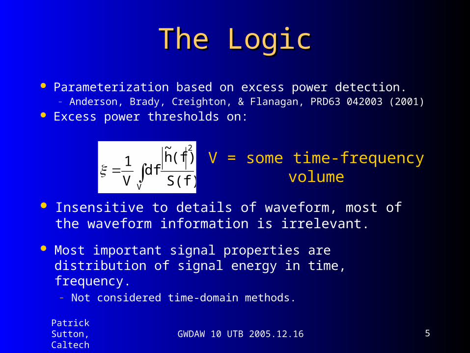
The LogicThe Logic

Most important signal properties are distribution of signal energy in time, frequency.

– Not considered time-domain methods.

V

2

S(f)

(f)h~

df V

1

V = some time-frequencyvolume

Parameterization based on excess power detection.– Anderson, Brady, Creighton, & Flanagan, PRD63 042003 (2001)

Excess power thresholds on:

Insensitive to details of waveform, most of the waveform information is irrelevant.


GWDAW 10 UTB 2005.12.16 6

Graphical ExampleGraphical Example(Heuristic)(Heuristic)

Characterise GWBs by these parameters:

– duration– central frequency– bandwidth

freq

uenc

ytimebest

match

Excess power search with various rectangular time-frequency tiles.

Overlap of signal with tile determined by signal duration, central frequency, bandwidth.


GWDAW 10 UTB 2005.12.16 7

Energy DistributionsEnergy Distributions

This is signal energy, not physical energy ( [th]2). Independent of polarization gauge choice.

Define duration, central frequency, bandwidth in terms of distribution of signal energy in time & frequency.

Energy distributions:

2

22

FDh

(f)h~

(f)h~

2 (f)ρ

frequency domain

2

22

TDh

(t)h(t)h (t)ρ time domain


GWDAW 10 UTB 2005.12.16 8

Energy Dist. (cont’d)Energy Dist. (cont’d)

0

22222

(f)h~

(f)h~

df(t)h(t)hdt h

1 (f)ρ df(t)ρdt FD

0

TD

Normalization factor is just hrss2 (Parseval’s theorem):

Normalized like probability distributions:


GWDAW 10 UTB 2005.12.16 9

Time-Domain MomentsTime-Domain Moments

Standard choice in signal-processing literature.

t(t)ρdt t TD

-

2TD

-

222 )-(t (t)ρdt tt

mean~ st dev

nTD

-

n t(t)ρdt t

Use lowest-order moments of energy distribution.

generalmoment

central time(not used)

duration


GWDAW 10 UTB 2005.12.16 10

Frequency-Domain MomentsFrequency-Domain Moments

Same thing:

f (f)ρ df fφ FD

0

nFD

0

n f (f)ρ df f

2FD

0

222 φ)-(f (f)ρ df ffΔφ

Can also consider higher moments of distributions.

bandwidth

centralfrequency

generalmoment


GWDAW 10 UTB 2005.12.16 11

Signals cannot have both arbitrarily small bandwidth and duration simultaneously:

Not the quantum-mechanics result (=1), because these are real signals

– Hilberg & Rothe, Information and Control 18 103 (1971).

Uncertainty PrincipleUncertainty Principle

.0.590106..Γ4π

ΓΔφ Δτ ,


GWDAW 10 UTB 2005.12.16 12

Uncertainty Principle(s)Uncertainty Principle(s)

Quantum-mechanics type argument implies second frequency-dependent uncertainty principle:

4π

1φΔφ Δτ 22

physical

not allowed


GWDAW 10 UTB 2005.12.16 13

The CheeseThe Cheese

duration

bandwidth

frequencyUncertainty relations:

From LIGO (approximate):

102 Hz < < 103 Hz 10-1 Hz < < 103 Hz 10-4 s < < 1 s

~ 0.1

Detectable physical signals live in here

“LIGO cheese”

= 103Hz

= 1s

(log-log-log plot)

= 103Hz

O(0.1)Δφ Δτ


GWDAW 10 UTB 2005.12.16 14

Spanning the CheeseSpanning the Cheese

Should be able to detect signals throughout the cheese. Want to be able to test efficiency at any point in the

cheese.– Astrophysical catalogs insufficient– So are sine-Gaussians and Gaussians used for most LIGO tuning.

Need waveform family that spans the cheese.– Current simulations (LIGO, LIGO-Virgo): band-limited white-

noise bursts.


GWDAW 10 UTB 2005.12.16 15

(LIGO cheese, top-down view)

S2 Sims: Bandwidth vs DurationS2 Sims: Bandwidth vs Duration

S2 simulations hug the “minimum uncertainty” side of the cheese.

Cover only a small portion of the signal space accessible with LIGO. unphysical

region

physical region

Gaussians

Lazarus BHMergers

sine-Gaussians

~ 0.1


GWDAW 10 UTB 2005.12.16 16

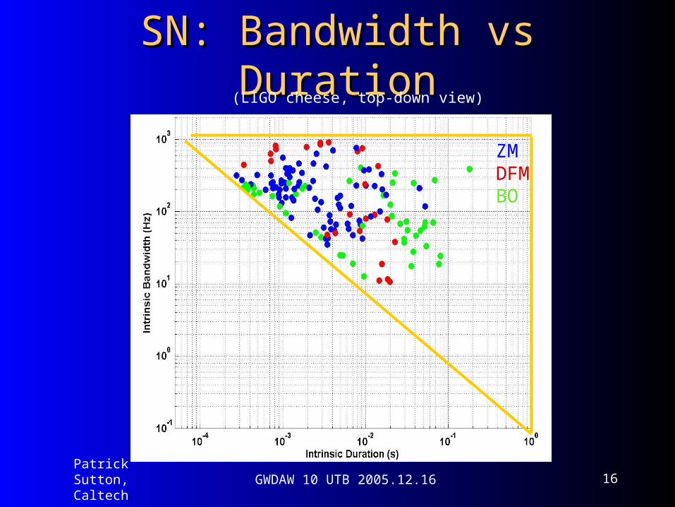
SN: Bandwidth vs DurationSN: Bandwidth vs Duration

ZMDFMBO

(LIGO cheese, top-down view)


GWDAW 10 UTB 2005.12.16 17

SN: Frequency vs BandwidthSN: Frequency vs Bandwidth

ZMDFMBO


GWDAW 10 UTB 2005.12.16 18

Chirplets & Maximum EntropyChirplets & Maximum Entropy

Need family of waveforms that spans the cheese– Continuous parameters to get any

No physical principle to specify such a family. Use mathematical principle to motivate choice of

waveform family: maximum entropy


GWDAW 10 UTB 2005.12.16 19

Waveform EntropyWaveform Entropy

Derive and h+, h× with maximum entropy subject to constraints on duration, bandwidth, frequency.

– Solution turns out to be Gaussian-modulated chirps

Shannon entropy for distribution (x) (x can be time or frequency):

– A measure of the “probability” of generating by randomly distributing energy in time or frequency.

– A measure of the amount of structure in .

ρ(x)ln ρ(x)dx entropy


GWDAW 10 UTB 2005.12.16 20

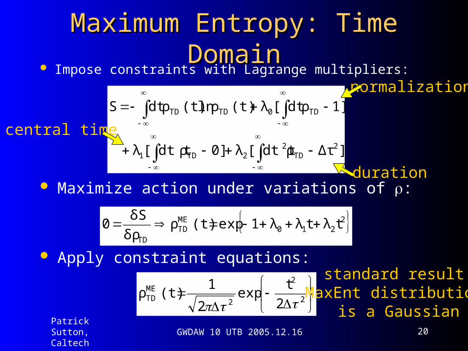
Maximum Entropy: Time DomainMaximum Entropy: Time Domain Impose constraints with Lagrange multipliers:

2210METD

TD

tλtλλ 1exp(t)ρδρ

δS0

Maximize action under variations of :

]Δτρdt t[λ 0]ρdt t [λ

1]ρdt [λ (t)ρln (t)ρdt S

2TD

22TD1

TD0TDTD

Apply constraint equations:

2

2

2

METD 2

texp

2

1(t)ρ

standard result:MaxEnt distribution

is a Gaussian

central time

duration

normalization


GWDAW 10 UTB 2005.12.16 21

Time-Domain SolutionTime-Domain Solution

High entropy waveforms: h+ and h× are phase-shifted versions of each other.

tih

2

2

4 2

MEME

4

texp

2)(t)ih(h

(t) is an arbitraryreal function of time

Corresponding waveform (general solution):


GWDAW 10 UTB 2005.12.16 22

i t 2 it

4

i1exp

2

h)(t)ih(h 2

24 2

MEME

Repeat maximum-entropy procedure in frequency domain to solve for (t). Approximate solution:

Solution: ChirpletsSolution: Chirplets

This is a chirplet: a Gaussian-modulated sinusoid with linearly sweeping frequency.

Chirp parameter related to bandwidth:

arbitrary phase

22

2

4

1

>0


GWDAW 10 UTB 2005.12.16 23

i t 2 it

4

i1exp

2

h)(t)ih(h 2

24 2

MEME

Chirplet contains sine-Gaussians, Gaussians as special cases:

Solution: ChirpletsSolution: Chirplets

= 0 Gaussian = 0 sine/cosine-Gaussian Setting =0 gives ~minimal-uncertainty waveforms.


GWDAW 10 UTB 2005.12.16 24

Metric in the CheeseMetric in the Cheese(in progress)(in progress)

Last ingredient: a measure of distance in the cheese (a metric).

– Are two signals are close or far apart?– How closely should we space injections

in frequency, bandwidth, and duration?– How rapidly should sensitivity vary?

We have a simple parametrization of the space of GWBs (the cheese).

We have a waveform family that spans the cheese (chirplets).


GWDAW 10 UTB 2005.12.16 25

Line of ThoughtLine of Thought

Study variation of detection statistic with changing parameters– Changing tile: : Ambiguity function - density of tiling for

guaranteed minimal sensitivity.

– Changing signal: : Variation in sensitivity over the cheese for fixed tiling (injection density).

Excess power detection statistic:– Tile with parameters .– Signal with cheese parameters = (,,).

S(f)

(f)h~

df V

1

2


GWDAW 10 UTB 2005.12.16 26

ExampleExample

2

22

2

2F/2F

F/2-F

T/2

T/2- 222

2exp

)(

1dfdt

FT

1

t

ft

fS

Detection statistic:

freq

uenc

y

time

F

T

F

Chirplet at = (,,) Rectangular tiles = (F,F,T)

– If tile is too large we include excess noise.

– If tile is too small we miss signal power.

Study behaviour numerically.


GWDAW 10 UTB 2005.12.16 27

SummarySummary

Future: Investigate sensitivity of various detection algorithms over

the cheese.– How well do predict sensitivity?– Are additional parameters needed?– Does it work for time-domain methods?

Derive ``metric.’’

Proposed a simple parametrization of the space of GWBs.– Based on excess power searches.

Derived maximum-entropy waveform family that spans the cheese (chirplets).


GWDAW 10 UTB 2005.12.16 28

AcknowledgementsAcknowledgements

Albert Lazzarini, Shourov Chatterji, Duncan Brown for many fruitful conversations.

1 Characterising the Space of Gravitational-Wave Bursts Patrick J. Sutton California Institute of...

Documents

Transcript of 1 Characterising the Space of Gravitational-Wave Bursts Patrick J. Sutton California Institute of...