1 Chapter 2 THE MATHEMATICS OF OPTIMIZATION Copyright ©2005 by South-Western, a division of Thomson...

1

Chapter 2

THE MATHEMATICS OF OPTIMIZATION

Copyright ©2005 by South-Western, a division of Thomson Learning. All rights reserved.

2

The Mathematics of Optimization

• Many economic theories begin with the assumption that an economic agent is seeking to find the optimal value of some function– consumers seek to maximize utility– firms seek to maximize profit

• This chapter introduces the mathematics common to these problems

3

Maximization of a Function of One Variable

• Simple example: Manager of a firm wishes to maximize profits

)(qf

= f(q)

Quantity

*

q*

Maximum profits of* occur at q*

4


• The manager will likely try to vary q to see where the maximum profit occurs– an increase from q1 to q2 leads to a rise in

= f(q)

Quantity

*

q*

1

q1

2

q2

0q

5


• If output is increased beyond q*, profit will decline– an increase from q* to q3 leads to a drop in

= f(q)

Quantity

*

q*

0q

3

q3

6

Derivatives

• The derivative of = f(q) is the limit of /q for very small changes in q

h

qfhqf

dq

df

dq

dh

)()(lim 11

0

• The value of this ratio depends on the value of q1

7

Value of a Derivative at a Point

• The evaluation of the derivative at the point q = q1 can be denoted

1qqdq

d

• In our previous example,

01

qqdq

d0

3

qqdq

d0

*qqdq

d

8

First Order Condition for a Maximum

• For a function of one variable to attain its maximum value at some point, the derivative at that point must be zero

0 *qq

dq

df

9

Second Order Conditions• The first order condition (d/dq) is a

necessary condition for a maximum, but it is not a sufficient condition

Quantity

*

q*

If the profit function was u-shaped,the first order condition would resultin q* being chosen and wouldbe minimized

10

Second Order Conditions

• This must mean that, in order for q* to be the optimum,

*qqdq

d

for 0 and *qq

dq

d

for 0

• Therefore, at q*, d/dq must be decreasing

11

Second Derivatives

• The derivative of a derivative is called a second derivative

• The second derivative can be denoted by

)(" or or 2

2

2

2

qfdq

fd

dq

d

12

Second Order Condition

• The second order condition to represent a (local) maximum is

0)("*

*

2

2

qqqq

qfdq

d

13

Rules for Finding Derivatives

0 then constant, a is If 1. dx

dbb

)(')]([

then constant, a is If 2. xbfdx

xbfdb

1 then constant, is If 3. bb

bxdx

dxb

xdx

xd 1ln 4.

14


aaadx

da xx

constantany for ln 5.

– a special case of this rule is dex/dx = ex

15


)(')(')]()([

6. xgxfdx

xgxfd

)()(')(')()]()([

7. xgxfxgxfdx

xgxfd

• Suppose that f(x) and g(x) are two functions of x and f’(x) and g’(x) exist

• Then

16


0)( that provided

)]([

)(')()()(')()(

8.2

xgxg

xgxfxgxf

dx

xgxf

d

17


dz

dg

dx

df

dz

dx

dx

dy

dz

dy 9.

• If y = f(x) and x = g(z) and if both f’(x) and g’(x) exist, then:

• This is called the chain rule. The chain rule allows us to study how one variable (z) affects another variable (y) through its influence on some intermediate variable (x)

18


axaxaxax

aeaedx

axd

axd

de

dx

de

)(

)( 10.

• Some examples of the chain rule include

)ln()ln()(

)(

)][ln()][ln( 11. axaaax

dx

axd

axd

axd

dx

axd

xx

xdx

xd

xd

xd

dx

xd 22

1)(

)(

)][ln()][ln( 12.

2

2

2

22

19

Example of Profit Maximization• Suppose that the relationship between

profit and output is

= 1,000q - 5q2

• The first order condition for a maximum is

d/dq = 1,000 - 10q = 0

q* = 100

• Since the second derivative is always -10, q = 100 is a global maximum

20

Functions of Several Variables

• Most goals of economic agents depend on several variables

– trade-offs must be made

• The dependence of one variable (y) on a series of other variables (x1,x2,…,xn) is denoted by

),...,,( nxxxfy 21

21

• The partial derivative of y with respect to x1 is denoted by

Partial Derivatives

1

111

ffx

f

x

yx or or or

• It is understood that in calculating the partial derivative, all of the other x’s are held constant

22

• A more formal definition of the partial derivative is

Partial Derivatives

h

xxxfxxhxf

x

f nn

hxx n

),...,,(),...,,(lim

2121

0,...,1 2

23

Calculating Partial Derivatives

2122

2111

2221

2121

2

2

cxbxfx

f

bxaxfx

f

cxxbxaxxxfy

and

then ,),( If 1.

2121

21

2

2

1

1

21

bxaxbxax

bxax

befx

faef

x

fexxfy

and

then If 2. ,),(

24

Calculating Partial Derivatives

2

2

21

1

1

2121

x

bf

x

f

x

af

x

fxbxaxxfy

and

then If 3. ,lnln),(

25

Partial Derivatives

• Partial derivatives are the mathematical expression of the ceteris paribus assumption– show how changes in one variable affect

some outcome when other influences are held constant

26

Partial Derivatives

• We must be concerned with how variables are measured– if q represents the quantity of gasoline

demanded (measured in billions of gallons) and p represents the price in dollars per gallon, then q/p will measure the change in demand (in billiions of gallons per year) for a dollar per gallon change in price

27

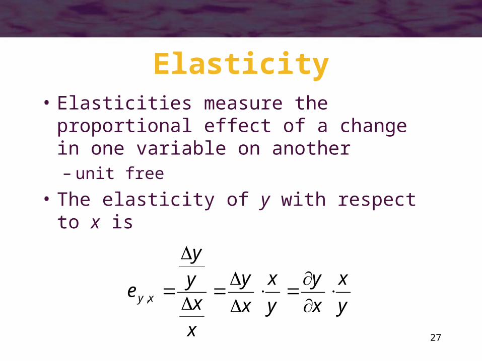
Elasticity• Elasticities measure the proportional

effect of a change in one variable on another– unit free

• The elasticity of y with respect to x is

y

x

x

y

y

x

x

y

xx

yy

e xy

,

28

Elasticity and Functional Form• Suppose that

y = a + bx + other terms

• In this case,

bxa

xb

y

xb

y

x

x

ye xy ,

• ey,x is not constant

– it is important to note the point at which the elasticity is to be computed

29

Elasticity and Functional Form

• Suppose that

y = axb

• In this case,

bax

xabx

y

x

x

ye

bb

xy

1,

30

Elasticity and Functional Form

• Suppose that

ln y = ln a + b ln x

• In this case,

x

yb

y

x

x

ye xy ln

ln,

• Elasticities can be calculated through logarithmic differentiation

31

Second-Order Partial Derivatives

• The partial derivative of a partial derivative is called a second-order partial derivative

ijijj

i fxx

f

x

xf

2)/(

32

Young’s Theorem

• Under general conditions, the order in which partial differentiation is conducted to evaluate second-order partial derivatives does not matter

jiij ff

33

Use of Second-Order Partials• Second-order partials play an important

role in many economic theories• One of the most important is a variable’s

own second-order partial, fii

– shows how the marginal influence of xi on y(y/xi) changes as the value of xi increases

– a value of fii < 0 indicates diminishing marginal effectiveness

34

Total Differential• Suppose that y = f(x1,x2,…,xn)

• If all x’s are varied by a small amount, the total effect on y will be

n

n

dxx

fdx

x

fdx

x

fdy

...2

2

1

1

nndxfdxfdxfdy ...2211

35

First-Order Condition for a Maximum (or Minimum)

• A necessary condition for a maximum (or minimum) of the function f(x1,x2,…,xn) is that dy = 0 for any combination of small changes in the x’s

• The only way for this to be true is if0...21 nfff

• A point where this condition holds is called a critical point

36

Finding a Maximum• Suppose that y is a function of x1 and x2

y = - (x1 - 1)2 - (x2 - 2)2 + 10

y = - x12 + 2x1 - x2

2 + 4x2 + 5

• First-order conditions imply that

042

022

2

2

1

1

xx

y

xx

y

OR2

1

2

1

*

*

x

x

37

Production Possibility Frontier

• Earlier example: 2x2 + y2 = 225

• Can be rewritten: f(x,y) = 2x2 + y2 - 225 = 0

• Because fx = 4x and fy = 2y, the opportunity cost trade-off between x and y is

y

x

y

x

f

f

dx

dy

y

x 2

2

4

38

Implicit Function Theorem• It may not always be possible to solve

implicit functions of the form g(x,y)=0 for unique explicit functions of the form y = f(x)– mathematicians have derived the necessary

conditions– in many economic applications, these

conditions are the same as the second-order conditions for a maximum (or minimum)

39

The Envelope Theorem

• The envelope theorem concerns how the optimal value for a particular function changes when a parameter of the function changes

• This is easiest to see by using an example

40


• Suppose that y is a function of x

y = -x2 + ax

• For different values of a, this function represents a family of inverted parabolas

• If a is assigned a specific value, then y becomes a function of x only and the value of x that maximizes y can be calculated

41


Value of a Value of x* Value of y* 0 0 0 1 1/2 1/4 2 1 1 3 3/2 9/4 4 2 4 5 5/2 25/4 6 3 9

Optimal Values of x and y for alternative values of a

42


0

1

2

3

4

5

6

7

8

9

10

0 1 2 3 4 5 6 7a

y*

As a increases,the maximal valuefor y (y*) increases

The relationshipbetween a and yis quadratic

43

The Envelope Theorem• Suppose we are interested in how y*

changes as a changes

• There are two ways we can do this– calculate the slope of y directly– hold x constant at its optimal value and

calculate y/a directly

44

The Envelope Theorem• To calculate the slope of the function, we

must solve for the optimal value of x for any value of a

dy/dx = -2x + a = 0

x* = a/2

• Substituting, we get

y* = -(x*)2 + a(x*) = -(a/2)2 + a(a/2)

y* = -a2/4 + a2/2 = a2/4

45

The Envelope Theorem• Therefore,

dy*/da = 2a/4 = a/2 = x*

• But, we can save time by using the envelope theorem– for small changes in a, dy*/da can be

computed by holding x at x* and calculating y/ a directly from y

46


y/ a = x

• Holding x = x*

y/ a = x* = a/2

• This is the same result found earlier

47

The Envelope Theorem• The envelope theorem states that the

change in the optimal value of a function with respect to a parameter of that function can be found by partially differentiating the objective function while holding x (or several x’s) at its optimal value

)}(*{*

axxa

y

da

dy

48

The Envelope Theorem• The envelope theorem can be extended to

the case where y is a function of several variables

y = f(x1,…xn,a)

• Finding an optimal value for y would consist of solving n first-order equations

y/xi = 0 (i = 1,…,n)

49

The Envelope Theorem• Optimal values for theses x’s would be

determined that are a function of a

x1* = x1*(a)

x2* = x2*(a)

xn*= xn*(a)

.

.

.

50

The Envelope Theorem• Substituting into the original objective

function yields an expression for the optimal value of y (y*)

y* = f [x1*(a), x2*(a),…,xn*(a),a]

• Differentiating yields

a

f

da

dx

x

f

da

dx

x

f

da

dx

x

f

da

dy n

n

...* 2

2

1

1

51

The Envelope Theorem• Because of first-order conditions, all terms

except f/a are equal to zero if the x’s are at their optimal values

• Therefore,

)}(*{*

axxa

f

da

dy

52

Constrained Maximization

• What if all values for the x’s are not feasible?– the values of x may all have to be positive– a consumer’s choices are limited by the

amount of purchasing power available

• One method used to solve constrained maximization problems is the Lagrangian multiplier method

53

Lagrangian Multiplier Method

• Suppose that we wish to find the values of x1, x2,…, xn that maximize

y = f(x1, x2,…, xn)

subject to a constraint that permits only certain values of the x’s to be used

g(x1, x2,…, xn) = 0

54


• The Lagrangian multiplier method starts with setting up the expression

L = f(x1, x2,…, xn ) + g(x1, x2,…, xn)

where is an additional variable called a Lagrangian multiplier

• When the constraint holds, L = f because g(x1, x2,…, xn) = 0

55

Lagrangian Multiplier Method• First-Order Conditions

L/x1 = f1 + g1 = 0

L/x2 = f2 + g2 = 0

.

L/xn = fn + gn = 0

.

.

L/ = g(x1, x2,…, xn) = 0

56


• The first-order conditions can generally be solved for x1, x2,…, xn and

• The solution will have two properties:– the x’s will obey the constraint– these x’s will make the value of L (and

therefore f) as large as possible

57

Lagrangian Multiplier Method• The Lagrangian multiplier () has an

important economic interpretation

• The first-order conditions imply that

f1/-g1 = f2/-g2 =…= fn/-gn =

– the numerators above measure the marginal benefit that one more unit of xi will have for the function f

– the denominators reflect the added burden on the constraint of using more xi

58

Lagrangian Multiplier Method• At the optimal choices for the x’s, the

ratio of the marginal benefit of increasing xi to the marginal cost of increasing xi should be the same for every x

is the common cost-benefit ratio for all of the x’s

i

i

x

x

of cost marginal

of benefit marginal

59

Lagrangian Multiplier Method• If the constraint was relaxed slightly, it

would not matter which x is changed

• The Lagrangian multiplier provides a measure of how the relaxation in the constraint will affect the value of y

provides a “shadow price” to the constraint

60

Lagrangian Multiplier Method• A high value of indicates that y could

be increased substantially by relaxing the constraint– each x has a high cost-benefit ratio

• A low value of indicates that there is not much to be gained by relaxing the constraint

=0 implies that the constraint is not binding

61

Duality

• Any constrained maximization problem has associated with it a dual problem in constrained minimization that focuses attention on the constraints in the original problem

62

Duality• Individuals maximize utility subject to a

budget constraint– dual problem: individuals minimize the

expenditure needed to achieve a given level of utility

• Firms minimize the cost of inputs to produce a given level of output– dual problem: firms maximize output for a

given cost of inputs purchased

63

Constrained Maximization• Suppose a farmer had a certain length of

fence (P) and wished to enclose the largest possible rectangular shape

• Let x be the length of one side• Let y be the length of the other side• Problem: choose x and y so as to maximize

the area (A = x·y) subject to the constraint that the perimeter is fixed at P = 2x + 2y

64

Constrained Maximization• Setting up the Lagrangian multiplier

L = x·y + (P - 2x - 2y)

• The first-order conditions for a maximum are

L/x = y - 2 = 0

L/y = x - 2 = 0

L/ = P - 2x - 2y = 0

65

Constrained Maximization• Since y/2 = x/2 = , x must be equal to y

– the field should be square– x and y should be chosen so that the ratio of

marginal benefits to marginal costs should be the same

• Since x = y and y = 2, we can use the constraint to show that

x = y = P/4

= P/8

66

Constrained Maximization• Interpretation of the Lagrangian multiplier

– if the farmer was interested in knowing how much more field could be fenced by adding an extra yard of fence, suggests that he could find out by dividing the present perimeter (P) by 8

– thus, the Lagrangian multiplier provides information about the implicit value of the constraint

67

Constrained Maximization• Dual problem: choose x and y to minimize

the amount of fence required to surround the field

minimize P = 2x + 2y subject to A = x·y

• Setting up the Lagrangian:

LD = 2x + 2y + D(A - xy)

68

Constrained Maximization• First-order conditions:

LD/x = 2 - D·y = 0

LD/y = 2 - D·x = 0

LD/D = A - x·y = 0

• Solving, we get

x = y = A1/2

• The Lagrangian multiplier (D) = 2A-1/2

69

Envelope Theorem & Constrained Maximization

• Suppose that we want to maximize

y = f(x1,…,xn;a)

subject to the constraint

g(x1,…,xn;a) = 0

• One way to solve would be to set up the Lagrangian expression and solve the first-order conditions

70

Envelope Theorem & Constrained Maximization

• Alternatively, it can be shown that

dy*/da = L/a(x1*,…,xn*;a)

• The change in the maximal value of y that results when a changes can be found by partially differentiating L and evaluating the partial derivative at the optimal point

71

Inequality Constraints

• In some economic problems the constraints need not hold exactly

• For example, suppose we seek to maximize y = f(x1,x2) subject to

g(x1,x2) 0,

x1 0, and

x2 0

72


• One way to solve this problem is to introduce three new variables (a, b, and c) that convert the inequalities into equalities

• To ensure that the inequalities continue to hold, we will square these new variables to ensure that their values are positive

73


g(x1,x2) - a2 = 0;

x1 - b2 = 0; and

x2 - c2 = 0

• Any solution that obeys these three equality constraints will also obey the inequality constraints

74

Inequality Constraints• We can set up the Lagrangian

L = f(x1,x2) + 1[g(x1,x2) - a2] + 2[x1 - b2] + 3[x2 -

c2]

• This will lead to eight first-order conditions

75

Inequality ConstraintsL/x1 = f1 + 1g1 + 2 = 0

L/x2 = f1 + 1g2 + 3 = 0

L/a = -2a1 = 0

L/b = -2b2 = 0

L/c = -2c3 = 0

L/1 = g(x1,x2) - a2 = 0

L/2 = x1 - b2 = 0

L/3 = x2 - c2 = 0

76

Inequality Constraints• According to the third condition, either a

or 1 = 0

– if a = 0, the constraint g(x1,x2) holds exactly

– if 1 = 0, the availability of some slackness of the constraint implies that its value to the objective function is 0

• Similar complemetary slackness relationships also hold for x1 and x2

77

Inequality Constraints• These results are sometimes called

Kuhn-Tucker conditions– they show that solutions to optimization

problems involving inequality constraints will differ from similar problems involving equality constraints in rather simple ways

– we cannot go wrong by working primarily with constraints involving equalities

78

Second Order Conditions - Functions of One Variable

• Let y = f(x)

• A necessary condition for a maximum is that

dy/dx = f ’(x) = 0

• To ensure that the point is a maximum, y must be decreasing for movements away from it

79


• The total differential measures the change in y

dy = f ’(x) dx

• To be at a maximum, dy must be decreasing for small increases in x

• To see the changes in dy, we must use the second derivative of y

80


• Note that d 2y < 0 implies that f ’’(x)dx2 < 0

• Since dx2 must be positive, f ’’(x) < 0

• This means that the function f must have a concave shape at the critical point

22 )(")("])('[

dxxfdxdxxfdxdx

dxxfdyd

81

Second Order Conditions - Functions of Two Variables

• Suppose that y = f(x1, x2)

• First order conditions for a maximum are

y/x1 = f1 = 0

y/x2 = f2 = 0

• To ensure that the point is a maximum, y must diminish for movements in any direction away from the critical point

82


• The slope in the x1 direction (f1) must be diminishing at the critical point

• The slope in the x2 direction (f2) must be diminishing at the critical point

• But, conditions must also be placed on the cross-partial derivative (f12 = f21) to ensure that dy is decreasing for all movements through the critical point

83


• The total differential of y is given by

dy = f1 dx1 + f2 dx2

• The differential of that function is

d 2y = (f11dx1 + f12dx2)dx1 + (f21dx1 + f22dx2)dx2

d 2y = f11dx12 + f12dx2dx1 + f21dx1 dx2 + f22dx2

2

• By Young’s theorem, f12 = f21 and

d 2y = f11dx12 + 2f12dx1dx2 + f22dx2

2

84


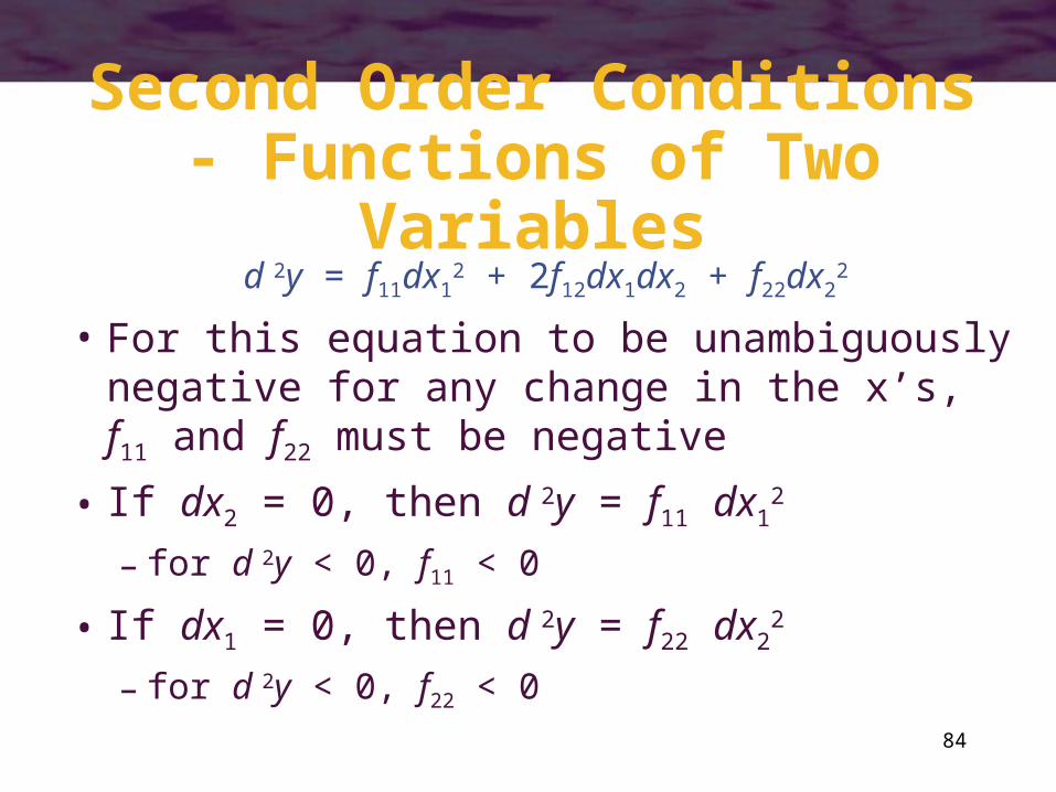
d 2y = f11dx12 + 2f12dx1dx2 + f22dx2

2

• For this equation to be unambiguously negative for any change in the x’s, f11 and f22 must be negative

• If dx2 = 0, then d 2y = f11 dx12

– for d 2y < 0, f11 < 0

• If dx1 = 0, then d 2y = f22 dx22

– for d 2y < 0, f22 < 0

85


d 2y = f11dx12 + 2f12dx1dx2 + f22dx2

2

• If neither dx1 nor dx2 is zero, then d 2y will be

unambiguously negative only if

f11 f22 - f122 > 0

– the second partial derivatives (f11 and f22) must be

sufficiently negative so that they outweigh any possible perverse effects from the cross-partial derivatives (f12 = f21)

86


• Suppose we want to choose x1 and x2 to maximize

y = f(x1, x2)

• subject to the linear constraintc - b1x1 - b2x2 = 0

• We can set up the Lagrangian

L = f(x1, x2) + (c - b1x1 - b2x2)

87


• The first-order conditions are

f1 - b1 = 0

f2 - b2 = 0

c - b1x1 - b2x2 = 0

• To ensure we have a maximum, we must use the “second” total differential

d 2y = f11dx12 + 2f12dx1dx2 + f22dx2

2

88

Constrained Maximization• Only the values of x1 and x2 that satisfy the

constraint can be considered valid alternatives to the critical point

• Thus, we must calculate the total differential of the constraint

-b1 dx1 - b2 dx2 = 0

dx2 = -(b1/b2)dx1

• These are the allowable relative changes in x1 and x2

89

Constrained Maximization• Because the first-order conditions imply

that f1/f2 = b1/b2, we can substitute and get

dx2 = -(f1/f2) dx1

• Since

d 2y = f11dx12 + 2f12dx1dx2 + f22dx2

2

we can substitute for dx2 and get

d 2y = f11dx12 - 2f12(f1/f2)dx1

2 + f22(f12/f2

2)dx12

90

Constrained Maximization• Combining terms and rearranging

d 2y = f11 f22

- 2f12f1f2 + f22f12 [dx1

2/ f22]

• Therefore, for d 2y < 0, it must be true that

f11 f22

- 2f12f1f2 + f22f12 < 0

• This equation characterizes a set of functions termed quasi-concave functions– any two points within the set can be joined

by a line contained completely in the set

91

Concave and Quasi-Concave Functions

• The differences between concave and quasi-concave functions can be illustrated with the function

y = f(x1,x2) = (x1x2)k

where the x’s take on only positive values and k can take on a variety of positive values

92

Concave and Quasi-Concave Functions

• No matter what value k takes, this function is quasi-concave

• Whether or not the function is concave depends on the value of k– if k < 0.5, the function is concave– if k > 0.5, the function is convex

93

Homogeneous Functions• A function f(x1,x2,…xn) is said to be

homogeneous of degree k if

f(tx1,tx2,…txn) = tk f(x1,x2,…xn)

– when a function is homogeneous of degree one, a doubling of all of its arguments doubles the value of the function itself

– when a function is homogeneous of degree zero, a doubling of all of its arguments leaves the value of the function unchanged

94

Homogeneous Functions

• If a function is homogeneous of degree k, the partial derivatives of the function will be homogeneous of degree k-1

95

Euler’s Theorem

• If we differentiate the definition for homogeneity with respect to the proportionality factor t, we get

ktk-1f(x1,…,xn) = x1f1(tx1,…,txn) + … + xnfn(x1,…,xn)

• This relationship is called Euler’s theorem

96

Euler’s Theorem

• Euler’s theorem shows that, for homogeneous functions, there is a definite relationship between the values of the function and the values of its partial derivatives

97

Homothetic Functions

• A homothetic function is one that is formed by taking a monotonic transformation of a homogeneous function– they do not possess the homogeneity

properties of their underlying functions

98


• For both homogeneous and homothetic functions, the implicit trade-offs among the variables in the function depend only on the ratios of those variables, not on their absolute values

99

Homothetic Functions• Suppose we are examining the simple,

two variable implicit function f(x,y) = 0

• The implicit trade-off between x and y for a two-variable function is

dy/dx = -fx/fy

• If we assume f is homogeneous of degree k, its partial derivatives will be homogeneous of degree k-1

100

Homothetic Functions• The implicit trade-off between x and y is

),(

),(

),(

),(1

1

tytxf

tytxf

tytxft

tytxft

dx

dy

y

x

yk

xk

• If t = 1/y,

1,

1,

1,'

1,'

yx

f

yx

f

yx

fF

yx

fF

dx

dy

y

x

y

x

101


• The trade-off is unaffected by the monotonic transformation and remains a function only of the ratio x to y

102

Important Points to Note:• Using mathematics provides a

convenient, short-hand way for economists to develop their models– implications of various economic

assumptions can be studied in a simplified setting through the use of such mathematical tools

103

Important Points to Note:• Derivatives are often used in economics

because economists are interested in how marginal changes in one variable affect another– partial derivatives incorporate the ceteris

paribus assumption used in most economic models

104

Important Points to Note:• The mathematics of optimization is an

important tool for the development of models that assume that economic agents rationally pursue some goal– the first-order condition for a maximum

requires that all partial derivatives equal zero

105

Important Points to Note:• Most economic optimization

problems involve constraints on the choices that agents can make– the first-order conditions for a

maximum suggest that each activity be operated at a level at which the ratio of the marginal benefit of the activity to its marginal cost

106

Important Points to Note:• The Lagrangian multiplier is used to

help solve constrained maximization problems– the Lagrangian multiplier can be

interpreted as the implicit value (shadow price) of the constraint

107

Important Points to Note:• The implicit function theorem illustrates

the dependence of the choices that result from an optimization problem on the parameters of that problem

108

Important Points to Note:• The envelope theorem examines

how optimal choices will change as the problem’s parameters change

• Some optimization problems may involve constraints that are inequalities rather than equalities

109

Important Points to Note:• First-order conditions are necessary

but not sufficient for ensuring a maximum or minimum– second-order conditions that describe

the curvature of the function must be checked

110

Important Points to Note:• Certain types of functions occur in

many economic problems– quasi-concave functions obey the

second-order conditions of constrained maximum or minimum problems when the constraints are linear

– homothetic functions have the property that implicit trade-offs among the variables depend only on the ratios of these variables

1 Chapter 2 THE MATHEMATICS OF OPTIMIZATION Copyright ©2005 by South-Western, a division of Thomson...

Documents

Transcript of 1 Chapter 2 THE MATHEMATICS OF OPTIMIZATION Copyright ©2005 by South-Western, a division of Thomson...