1 ANALYSIS OF INVENTORY MODEL Notes 1 of 2 By: Prof. Y.P. Chiu 2011 / 09 / 01.

1

ANALYSIS OF ANALYSIS OF

INVENTORY MODELINVENTORY MODEL

Notes 1 of 2Notes 1 of 2

By: Prof. Y.P. ChiuBy: Prof. Y.P. Chiu

2011 / 09 / 012011 / 09 / 01

2

§ I1 :§ I1 : Types of InventoriesTypes of Inventories

(A) Raw Materials(B) Components(C) Work in process(D) Finished goods

◇◇

§ I2 : Inventory Relevant § I2 : Inventory Relevant CostsCosts

(A) Holding Cost (B) Order Cost

(C) Penalty Cost (D) Outdate Cost

Analysis of Inventory ModelAnalysis of Inventory Model

3

§ I2(A) : Holding Cost§ I2(A) : Holding Cost

• Opportunity cost of alternative

investment

• Taxes and insurance

• Breakage, spoilage, deterioration, obsolescence

• Cost of physical space

Eg: 28% = cost of capital

2% = Taxes and insurance

6% = cost of storage

1% = breakage and spoilage 37% = Total interest charge

h = i ． c

◇◇

4

§ I2(B) : Order Cost§ I2(B) : Order Cost

Cost of procuring x items :

(fixed cost plus proportional cost)

0 x if cx K

0 x if 0 C(x)

◇◇

5

§ I2(C) : Penalty Cost§ I2(C) : Penalty Cost

• Cost when demand exceeds supply

( per unit of excess demand )

§ I2(D) : Outdate Cost§ I2(D) : Outdate Cost

• Cost when inventories spoiled (oroutdated)

( including cost of discarding the spoilage items )

◇◇

6

§ I3 : Motivation for Holding§ I3 : Motivation for Holding Inventories Inventories

1. Economies of Scale

2. Uncertainties． Excess demand

3. Speculation

4. Transportation

5. Smoothing

6. Logistics ． safety stock ． minimum purchasing

quantity

7. Control Costs ． record keeping &

． management costs

◇◇

7

§ I4 : Characteristics of § I4 : Characteristics of Inventory System Inventory System

(A) Demand ． Constant versus Variable ． Known versus Random

(B) Lead Time ． Zero, Constant, Variable, R

andom

(C) Review Time ． Continuous, Periodic

(D) Excess Demand ． Backordered, Lost

(E) Ordering Policy . (r,Q), (s,S), etc.

(F) Issuing Policy . FIFO, LIFO, etc.

(G) Changing Inventory ． Shelf life (expired), obsole

te

◇◇

8

§ I5 : § I5 : EOQ (Economic Order EOQ (Economic Order Quantity) Quantity)

Q

T

Slope = -

Inve

ntor

y( I

( t )

)

Fig.1

Time t

◇◇

9

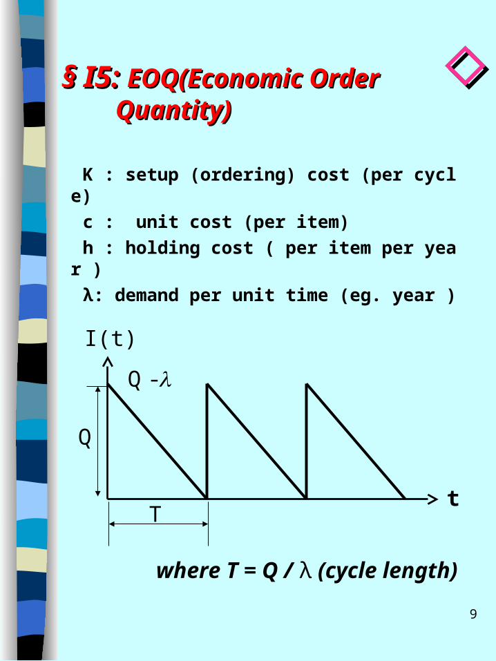
§ I5: § I5: EOQ(Economic Order EOQ(Economic Order Quantity) Quantity)

K : setup (ordering) cost (per cycle)

c : unit cost (per item)

h : holding cost ( per item per year )

λ: demand per unit time (eg. year )

Q

T

I(t)

t - Q

t

where T = Q / λ (cycle length)

◇◇

10

G(Q) = Inventory Costs per unit time (per year)

G(Q) = Gc(Q) / T = (K+cQ) / T + h • Q/2

T2)(QhcQ)(kGc(Q) /

Inventory Costs per cycle

T = Q / λ

……[Eq.5.1]

§ I5.1 : § I5.1 : Inventory Costs G(Q)Inventory Costs G(Q) in EOQ Model in EOQ Model

◇◇

11

2

QhcQ K

2

QhQcQ) (K G(Q)

Set up cost / unit time

Purchase cost / unit time

Holding cost / unit time

….[Eq.5.2]

§ I5.1 : Inventory Costs G(Q)§ I5.1 : Inventory Costs G(Q) in EOQ Model in EOQ Model

◇◇

12

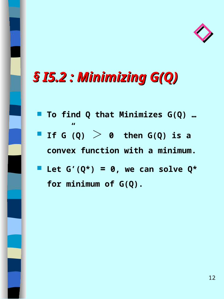
§ I5.2 : Minimizing G(Q)§ I5.2 : Minimizing G(Q)

To find Q that Minimizes G(Q) …

If G”(Q) ＞ 0 then G(Q) is a convex

function with a minimum.

Let G’(Q*) = 0, we can solve Q* for

minimum of G(Q).

◇◇

13

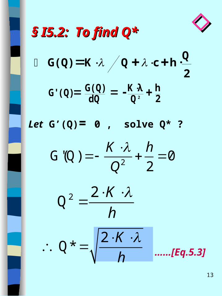
§ I5.2: To find Q*§ I5.2: To find Q*

2

QhcQ K G(Q)

2h

QλK

dQG(Q) (Q)G' -

2

Let G’(Q)= 0 , solve Q* ?

2G'(Q) 0

2

K h

Q

2 2Q

K

h

……[Eq.5.3]

◇◇

2 Q*

K

h

14

§ I§ I5.3 : EOQ ~ Discussion5.3 : EOQ ~ Discussion

EOQ model :

Balances order cost and holding cost

The basic model:

1. The demand rate is known and is constant λ items per unit time

2. Shortages are not permitted

3. No order lead time

4. Costs include ◆ setup (ordering) cost K per order ◆ holding cost h per item held

per unit time ◆ unit cost c per item ordered.

2Q*

K

h

15

§.§. I 5. I 5. ProblemsProblems & & Discussion Discussion

( ( # N4.1, N4.9# N4.1, N4.9 ) )

( ( # # S5.1S5.1, S5.2, S5.2 ) )

Preparation Time : 20 ~ 30 minutesPreparation Time : 20 ~ 30 minutesDiscussion : 15 ~ 25 minutesDiscussion : 15 ~ 25 minutes

16

§ I6 : Sensitivity§ I6 : Sensitivity

How cost increases if not using Q*

recall [Eq.5.2]

Drop λC for now

2Qh

Qk

(Q)G

hk22

*Qh*Q

k *GLet

2*Qh

*Qk

G(Q*)

1

C

if we use Q rather than Q*, then

17

§ I6 : § I6 : SensitivitySensitivity

*QQ

Q*Q

21

λK2h

2Q

hλK2

2Q1

hλk2

2Qh

Qλk

*G

(Q)G 1

(G*)*Q

QQ

*Q21 (Q)G

1

18

§.§. I 6. I 6. ProblemsProblems & & Discussion Discussion

( ( # C.1, # C.2# C.1, # C.2 ) )


19

§ I7 : § I7 : Order Lead TimeOrder Lead Time : : ττ To order “τ” time in advance. or to consider a reorder point (I.e. level of inventory = “R”)

(A) For τ < T

4 month

R=1040

Q*=3870

t

I(t)

T = 1.24 year

◇◇

20

Let τ = 4 months = 0.3333 year

R= λτ = 3120 （ 0.3333) = 1040

(B) When τ > T

(1) From the ratio τ / T (2) • Consider only the fractional

remainder (f-r) of the ratio.

• Convert this (f-r) back to

year.

(3) use R = λ * τ(f-r)

§ I7 : § I7 : Order Lead Time : τOrder Lead Time : τ◇◇

21

if τ = 6 weeks

Q*= 25

T =2.6 weeks

λ= 500 per year

( a ) τ / T = 6/ 2.6 = 2.31 periods

( b ) 0.31: fractional remainder 0.31 (2.6) / 52 = 0.0155 years

( c ) R= 500 (0.0155) = 7.75 ≒ 8

[Eg.7.1] ◇◇

22

(C) Summary : (1) EOQ FORMULA

hk2

Q*

(2) REORDER LEVEL

For τ< T, R =λτ

For τ> T, R =λ

where

eff

(3) Rules for Computing

If 2T > τ> T, then = τ- T

If 3T > τ> 2T, then = τ- 2T etc.

eff

§ I7 : § I7 : Order Lead Time : τOrder Lead Time : τ ◇◇

eff T

effeff

23

§.§.I 7. I 7. ProblemsProblems & & Discussion Discussion

( ( # N4.12, N4.14# N4.12, N4.14 N4.14-2N4.14-2 ) )


24

§ I8 : Model for Shortages§ I8 : Model for Shortages Permitted Permitted

SQS-λt

S/λ

Q/λ

Demand =λ

t

(a) Cycle length T T == Q/ λ Q/ λ;

hh : holding costs; pp : shortage costs/item/unit

time

(b) Shortage occurs for a time : (Q-S)/λ(Q-S)/λ

(c) Average amount of shortages :

[0+(Q-S)]/2[0+(Q-S)]/2

(d) Shortage cost : p(Q-S) / 2p(Q-S) / 2

25

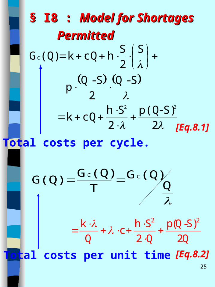
§ I8 : § I8 : Model for ShortagesModel for Shortages

Permitted Permitted

2S)-p(Q

2Sh

cQk

S-Q2

S-Qp

S2S

hcQk(Q)G

22

C

Total costs per cycle.

[Eq.8.2]

2 2k h S p(Q-S)c

Q 2 Q 2Q

Q

(Q)GT(Q)G

G(Q) CC

Total costs per unit time

[Eq.8.1]

26

02Q

S)-p(Q

Q

S)-p(Q

Q2

Sh

Q

k-

Q

G(Q)

0Q

S)-p(Q

Q

Sh

S

G(Q)

2Q

S)-p(Q

Q2

Shc

Q

kG(Q)

2

2

2

2

2

22

php

hk2*QT*

hpp

hk2 S*

php

hk2 Q*

[Eq.8.3a]

[Eq.8.3c]

[Eq.8.3b]

§ I8: Model for Shortages§ I8: Model for Shortages Permitted Permitted

[Eq.8.2]

27

§.§. I8. I8. Problems &Problems & Discussion Discussion

( ( # C.3# C.3 ) )


28

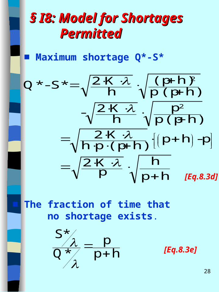
hp

hpK2

p-hph)(pph

K2

h)p(pp

hK2-

h)(p p

h)(phK2 S* -*Q

2

2

[Eq.8.3d]

■ The fraction of time that no shortage exists.

■ Maximum shortage Q*-S*

hpp

*Q

*S

[Eq.8.3e]

§ I8: Model for Shortages§ I8: Model for Shortages Permitted Permitted

29

A television manufacturing company produces its own speakers, which are used in production of its television sets. The television sets are assembled on a continuous line at the rate of 8,000 per month. The speakers are produced in batches because they do not warrant setting up a continuous production line, and relatively large quantities can be produce in a short time. The company is interested in determining when and how many to produce. Several costs must be considered:

[Eg. 8.1]

1.Each time a batch is produced, a setup cost of $12,000 is incurred. This cost includes the cost of “tooling up,” administrative costs, record-keeping, and so forth. Note that the existence of this cost argues for producing speakers in large batches.

30

2.The production of speakers in large batches leads to a large inventory. The estimated cost of keeping a speaker in stock is 30 cents / month. This cost includes the cost of capital tied up, storage space, insurance, taxes, protection, and so on. The existence of a storage or holding cost argues for producing small batches.

[Eg. 8.1]

3.The production cost of a single speaker (excluding the setup cost) is $10 and can be assumed to be a unit cost independent of the batch size produced. (In general, however, the unit production cost need not be constant and may decrease with batch size.)

31

4. Company policy prohibits deliberately planning for shortages of any of its components. However, a shortage of speakers occasionally crops up, and it has been estimated that each speaker that is not available when required costs 1.10 / month. This cost includes the cost of installing speakers after the television set is fully assembled, storage space, delayed revenue, record keeping, and so forth.

[Eg. 8.1]

K=$12,000/order λ=8000/month

h= $0.3/item/month c= $10/item

p=$1.10/item/month

unit of time = a month

Solution to [Eg.8.1]

32


2 k λ 2 12000 8000Q* h 0.3

25,298

25,298Q*T 3.16 monthλ 8,000

(A) E.O.Q

$276,980

.2

25,298 0.3

,$,$

T2

*Qh*cQk(Q)GC

163

298251000012

33

$87,590

3795800003795 225298 0.3

10 800025298

800012000

2*QhCλ

*Qλk G(Q*)

per unit of time → ie ”month” in this case


34

(B) When shortage permitted

p=$1.10 per speaker

k=$12,000 h = $0.3

λ=8000

Use [Eq.8.3 a]

28540 1.1

3.01.13.0

8000120002

php

hk2

Q*


Use [Eq.8.3b]

424,22hp

p

h

k2*

S

Use [Eq.8.3c]

T*= Q*/λ=28540 / 8000 = 3.57 (months)

35

Use [Eq.8.3d] Maximum shortage Q*-S*=6116

Time shortage occurs

( Q*-S*) / λ= 6116 / 8000

= 0.76 months

• Time no shortage occurs

S*/λ=22424/8000=2.8 months


36

(C) Discussion:

• When “shortage permitted”

S

Q

S/λ

T=Q/λ

Q-S t

37

Eg. from 8.1(b)

• When “shortage permitted”

Q*=28540 T* = Q*/λ= 3.57 month

S*=22424

*2Q*Q2S*)(h

c*Q

kT

(Q*)GG(Q*)2

C

2

-S*)*p(Q

2

S*)(h*cQK(Q*)G

22

C

72886

7216432000803643

28540

22424

1080008000

,$

$,$,$,$

2854021.1(6116)

20.3

2854012000

22

G(Q*)

38

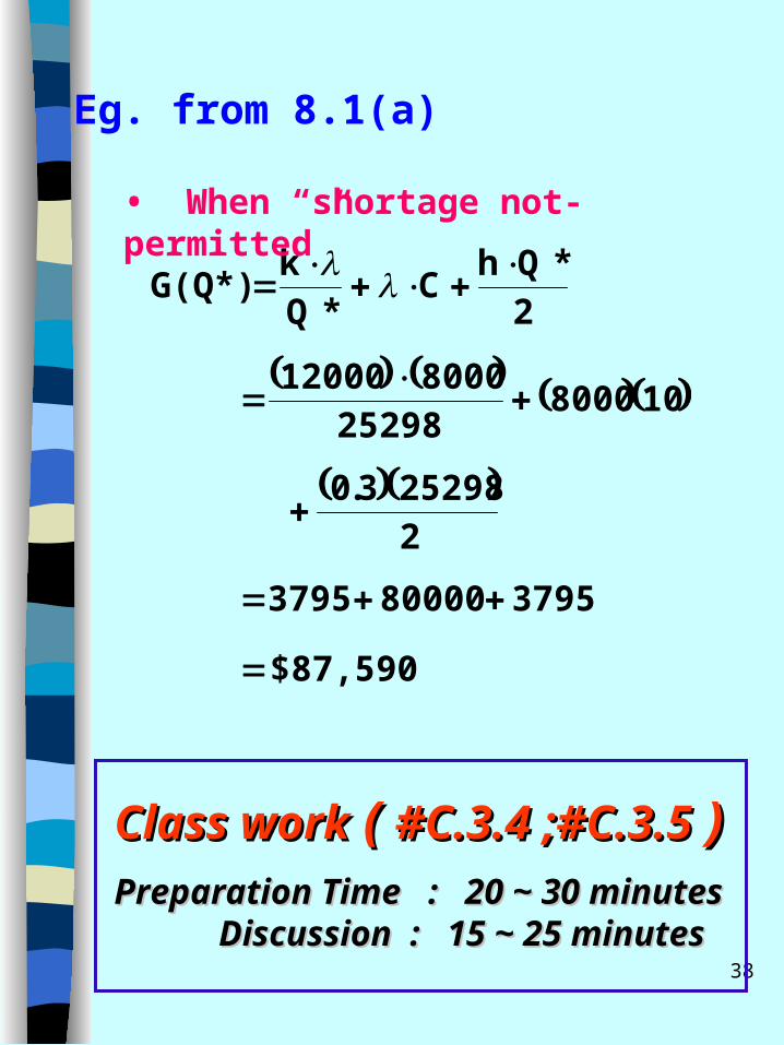
$87,590

3795800003795

.

2529812000

2*Qh

*Qk G(Q*)

2

2529830

1080008000

C

• When “shortage not-permitted”

Eg. from 8.1(a)

Class workClass work ( ( #C.3.4 ;#C.3.5#C.3.4 ;#C.3.5 ) ) Preparation Time : 20 ~ 30 minutesPreparation Time : 20 ~ 30 minutes

Discussion : 15 ~ 25 minutesDiscussion : 15 ~ 25 minutes

39

T1 T2

T

t

H

I(t)

§ I9 : Inventory Management for § I9 : Inventory Management for Finite Production RateFinite Production Rate

• Inventory Levels for Finite Production Rate Model

Fig.9.1

Slope=P- λ

Slope= - λ

40

P : production rate (per unit time)λ: demand rate (per unit time)

P >λ

T1 T2t

H

I(t) T

Q

P-1 QH

PQ

-PH

T -P TH

PQ T TP Q

Q T T Q

11

11

§ I9 : Finite Production Rate§ I9 : Finite Production Rate

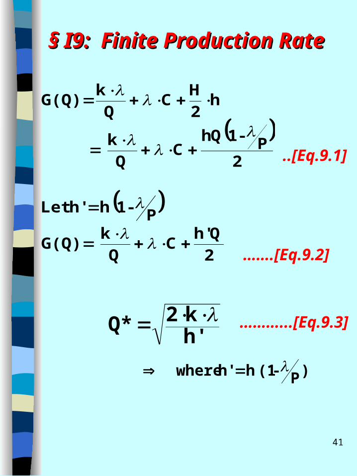
41

)P-(1 h h' where

h'k2Q*

………...[Eq.9.3]

2

Qh'

Q

k G(Q)

P-1 h h'Let

2

P-1Q

Q

k

h2

H

Q

k G(Q)

C

hC

C

..[Eq.9.1]

…….[Eq.9.2]

§ I9: Finite Production Rate§ I9: Finite Production Rate

42

A local company produces a programmable EPROM for several industrial clients. It has experienced a relatively flat demand of 2,500 units per year for the product. The EPROM is produced at a rate of 10,000 units per year. The accounting department has estimated that it costs $50 to initiate a production run, each unit cost the company $2 to manufacture, and the cost of holding is based on a 30 % annual interest rate. Determine the optimal size of a production run, the length of each production run, and the average annual cost of holding and setup. What is the maximum level of the on-hand inventory of the EPROMs?

[Eg. 9.1][Eg. 9.1]

43

λ = 2500 / year

P = 10,000 /year

K = $50 / setup

c = $ 2 / unit

i =30%

unit /year / 0.6 $ (30%) ($2) ci h

45.0100002500

16.0

P1- h h'

Solution to [Eg.9.1] :

～ Finite Production Rate ～

• Use [Eq.9.3]

units 745 *Q

.502

h'k2

Q*

450

2500

44

years...T -T T

years0.0745 10000745

P*Q

T

units .P-1*Q H

years.2500745

*Q

*T

12

1

units 745 *Q

22350074502980

5592501745

2980

Solution to [Eg.9.1] :

～ Finite Production Rate ～

• Use [Eq.9.2] 2Qh'

Qk

G(Q)

C

setup cost / year holding cost / year

167.785

745250050

Qλk

167.625

27450.45

2Qh' •

•

45

t1 t2

t3

Time

T

S

I(t)

P-λ-λ

B

P-λ

t4

T

Q

-λ

t2t1 t3

§ I9.1: Finite Production Rate§ I9.1: Finite Production Rate with Backorderingwith Backordering

*

* *

* (1) (2)

(3)

12

12

1

1

2b

KK b hQ

bhP

hB

PS

h b h

hK Pb b

Qhb h P

46

§.§. I 9. I 9. Problems &Problems & Discussion Discussion


( ( # N4.17 ; N4.20 # N4.17 ; N4.20 ))

# C.3.8 ; #C.3.9# C.3.8 ; #C.3.9

( ( # S5.3 ;# S5.3 ; S5.4 ; S5.7 S5.4 ; S5.7 ))

47

C 0 = 0.30C 1=0.29

C 2=0.28

500 1,000 Q

C(Q

)§ I10 : All-Units Discount § I10 : All-Units Discount Inventory ModelInventory Model

Fig.10.1 All-units Discount order cost function

All Units Discount

0.30Q for 0 ≦ Q ＜ 500

C(Q)= 0.29Q for 500 ≦ Q ＜ 1000

0.28Q for 1000 ≦ Q

﹛

◇◇

48

• Assume λ= 600 k = $ 8

h = 0.20( Cj ) = (0.2)(0.3)

= (0.2)(0.29)

= (0.2)(0.28)

)[1000, Q

[500,1000) Q

) 500 0, [ Q

(A)Use [Eq.5.3] to find optimal for each Qj-intervals.

41428.0

40629.0

4003.0

0.2k2

Q

0.2k2

Q

0.2

k2Q

(2)

(1)

(0)

§ I10 : All-Units § I10 : All-Units Discount Discount Inventory ModelInventory Model

◇◇

49

G0(Q) Vaild G1(Q) Valid G2(Q) ValidG(Q)

$230

$220

$210

$190

$180Q

Q(1) ≒ 406 ∴ Q(1)* = 500

Q(2) ≒ 414 ∴ Q(2)* = 1000

100 200 300 400 500 600 700 800 900 1000

§ I10 : All-Units Discount § I10 : All-Units Discount Inventory ModelInventory Model

◇◇

50

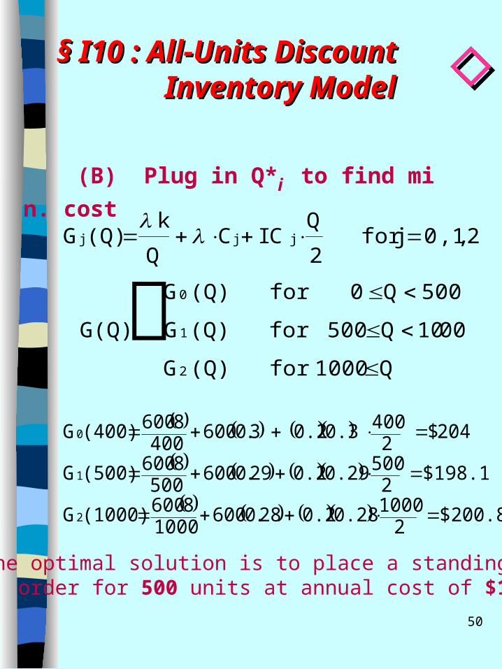
(B) Plug in Q*i to find min. cost

Q 1000for (Q) G

0010 Q 500for (Q) G G(Q)

500 Q 0 for (Q) G

2 , ,1 0jfor 2

Q C I C

Q

k (Q) G

2

1

0

jjj

﹛ $200.8

21000 0.280.2 28.0600

10008600 (1000)G

$198.1 2

500 0.290.2 29.0600500

8600 (500)G

204$ 2

400 0.30.2 3.0600400

8600 (400)G

2

1

0

∴The optimal solution is to place a standing order for 500 units at annual cost of $198.1

§ I10 : All-Units Discount § I10 : All-Units Discount Inventory ModelInventory Model ◇◇

51

§.§. I10. I10. Problems &Problems & Discussion Discussion


( ( # N4.22 ; N4.24 # N4.22 ; N4.24 ) )

( ( # S5.9# S5.9 ))

52

500 1000

C0=0.3

C1=0.29

C3=0.28

150

295

C(Q

)

Q

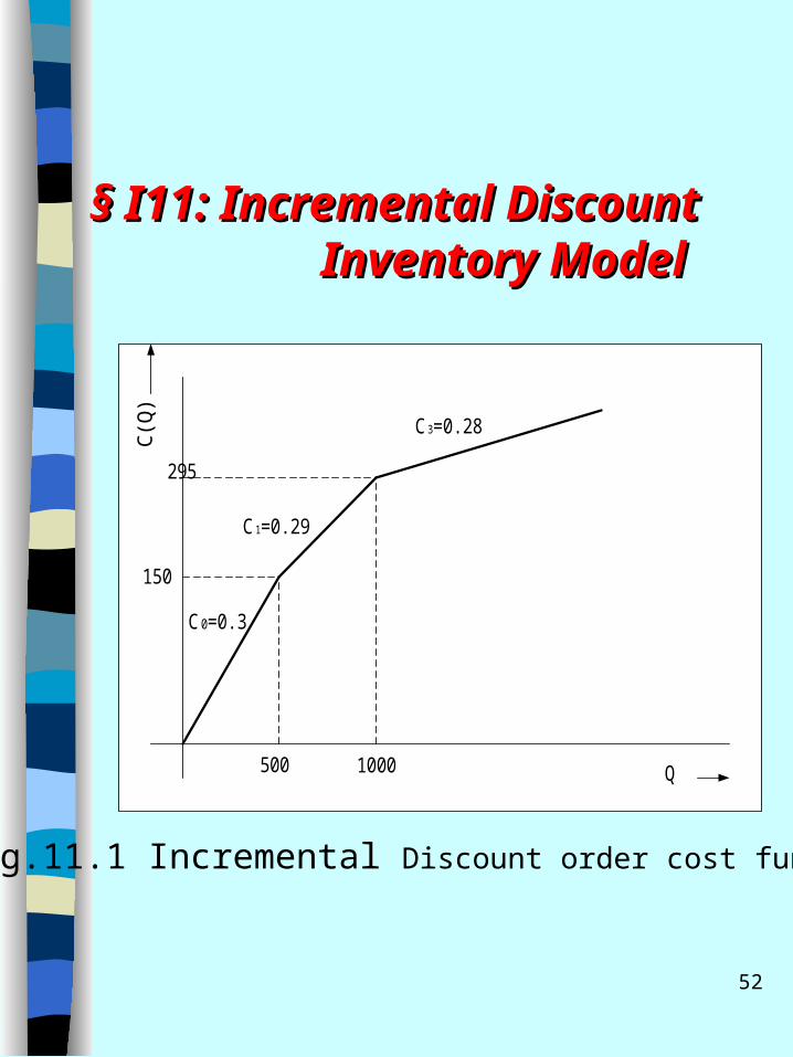
§ I11: Incremental Discount § I11: Incremental Discount Inventory ModelInventory Model

Fig.11.1 Incremental Discount order cost function

53

Q 1000 for 1000)-0.28(Q$295

1000 Q 500 for 500)-0.29(Q$150 C(Q)

500 Q 0 for 0.3Q $

﹛2Qh

CλQλk

G(Q)j

j

(A)

(B)

Q 000 1 for Q15$0.28

1000 Q 500 for Q5 $0.29 Q

C(Q)C 500 Q 0 for $0.3

j

﹛


54

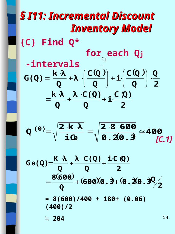
(C) Find Q* for each Qj -intervals

2

Q)Ci

Q

C(Q)λ

Q

λk

2

Q

Q

QCi

Q

QCλ

Q

λk G(Q)

(

4000.3 0.2

60082

iC

λk2 Q

0

(0)

2Q0.30.20.3600

Q

6008

2

Q)Ci

Q

C(Q)λ

Q

λK(Q)G0

(

[C.1]

Cj

= 8(600)/400 + 180+ (0.06)(400)/2

≒ 204


55

1k C(Q) i C(Q)

G (Q)Q Q 2

8 600 (0.2) 5 0.29Q5 600 0.29 QQ 2

4800 3000 174 0.5 0.029Q

Q Q

58.204$)(QG 519 Q

5190.029

7800Q

029.0

7800Q

Q

78000.029

0Q

78002(Q)"G

minimal 0029.0Q

7800-(Q)'G

Q029.05.174Q

7800(Q)G

(1)1

(1)

2

2

31

21

1

[C.2]


56

$208.8(1000)G

7020.02813800

Q 0.028Q

9000Q4800-

(Q)'G

0.028Q1.5Q

9000168

Q4800

20.28Q150.2

Q150.28600

Q6008

2C(Q)i

QC(Q)λ

QλK

(Q)G

2

(2)222

2

0001Q(2)

[C.3]

G(Q)

$220

$216

$212

$208

$204

$200

G0(Q) G1(Q)

G2(Q)

Q0*=400Q1*=519

Q2*=702

Q

100 200 300 400 500 700 1000


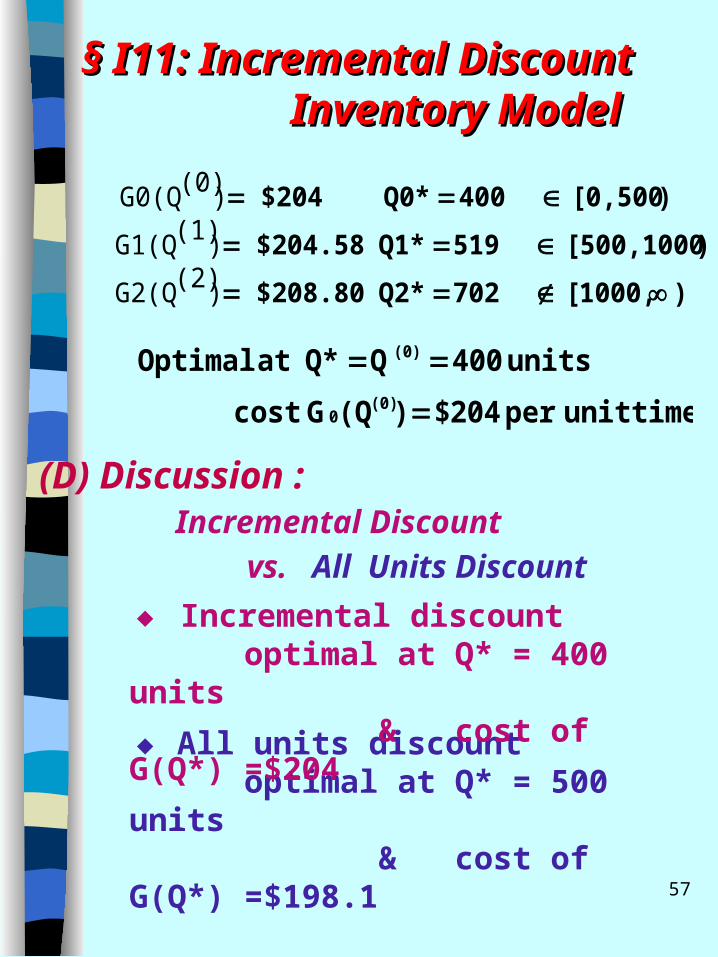
57

) 1000,[ 702Q2* $208.80

) 500,1000[ 519Q1* $204.58

) 0,500[ 400Q0* $204

)(2)G2(Q

)(1)G1(Q

)(0)G0(Q

(D) Discussion : Incremental Discount

vs. All Units Discount

◆ All units discount optimal at Q* = 500 units & cost of G(Q*) =$198.1

timeunit per $)(QGcost

units QQ*at Optimal(0)

0

(0)

204

400

◆ Incremental discount optimal at Q* = 400 units & cost of G(Q*) =$204


58

(E) Incremental solution technique:

one lowest the pick and *)G(Q compute

erval right ) [*Q each For (4)

*Q find to )G(Q (3)Use

[C(Q)/Q] i h Find (2)

C(Q)/Q& C(Q) Determine (1)

j

j

jj

j

int

• • There are other discount schedules.There are other discount schedules.


59

§.§. I11. I11. Problems &Problems &DiscussionDiscussion


( ( # N4.23 ; N4.35 # N4.23 ; N4.35 ) )

( ( # S5.14# S5.14 ))

The End ofThe End of Class NotesClass Notes

1 of 21 of 2

1 ANALYSIS OF INVENTORY MODEL Notes 1 of 2 By: Prof. Y.P. Chiu 2011 / 09 / 01.

Documents

Transcript of 1 ANALYSIS OF INVENTORY MODEL Notes 1 of 2 By: Prof. Y.P. Chiu 2011 / 09 / 01.