1. 01-18 Container-Throughput Forecasting in the Port of ...
18
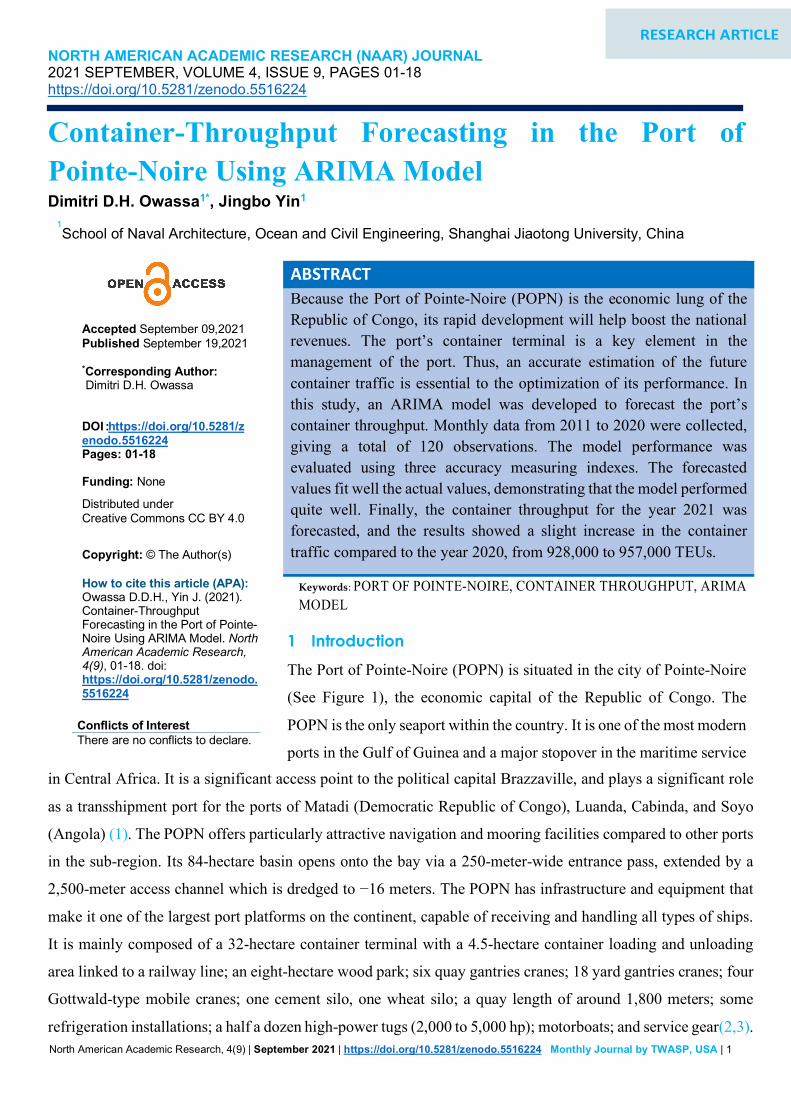
North American Academic Research, 4(9) | September 2021 | https://doi.org/10.5281/zenodo.5516224 Monthly Journal by TWASP, USA | 1 NORTH AMERICAN ACADEMIC RESEARCH (NAAR) JOURNAL 2021 SEPTEMBER, VOLUME 4, ISSUE 9, PAGES 01-18 https://doi.org/10.5281/zenodo.5516224 Container-Throughput Forecasting in the Port of Pointe-Noire Using ARIMA Model Dimitri D.H. Owassa 1* , Jingbo Yin 1 1 School of Naval Architecture, Ocean and Civil Engineering, Shanghai Jiaotong University, China ABSTRACT Because the Port of Pointe-Noire (POPN) is the economic lung of the Republic of Congo, its rapid development will help boost the national revenues. The port’s container terminal is a key element in the management of the port. Thus, an accurate estimation of the future container traffic is essential to the optimization of its performance. In this study, an ARIMA model was developed to forecast the port’s container throughput. Monthly data from 2011 to 2020 were collected, giving a total of 120 observations. The model performance was evaluated using three accuracy measuring indexes. The forecasted values fit well the actual values, demonstrating that the model performed quite well. Finally, the container throughput for the year 2021 was forecasted, and the results showed a slight increase in the container traffic compared to the year 2020, from 928,000 to 957,000 TEUs. Keywords: PORT OF POINTE-NOIRE, CONTAINER THROUGHPUT, ARIMA MODEL in Central Africa. It is a significant access point to the political capital Brazzaville, and plays a significant role as a transshipment port for the ports of Matadi (Democratic Republic of Congo), Luanda, Cabinda, and Soyo (Angola) (1). The POPN offers particularly attractive navigation and mooring facilities compared to other ports in the sub-region. Its 84-hectare basin opens onto the bay via a 250-meter-wide entrance pass, extended by a 2,500-meter access channel which is dredged to −16 meters. The POPN has infrastructure and equipment that make it one of the largest port platforms on the continent, capable of receiving and handling all types of ships. It is mainly composed of a 32-hectare container terminal with a 4.5-hectare container loading and unloading area linked to a railway line; an eight-hectare wood park; six quay gantries cranes; 18 yard gantries cranes; four Gottwald-type mobile cranes; one cement silo, one wheat silo; a quay length of around 1,800 meters; some refrigeration installations; a half a dozen high-power tugs (2,000 to 5,000 hp); motorboats; and service gear(2,3). RESEARCH ARTICLE Accepted September 09,2021 Published September 19,2021 * Corresponding Author: Dimitri D.H. Owassa DOI : https://doi.org/10.5281/z enodo.5516224 Pages: 01-18 Funding: None Distributed under Creative Commons CC BY 4.0 Copyright: © The Author(s) How to cite this article (APA): Owassa D.D.H., Yin J. (2021). Container-Throughput Forecasting in the Port of Pointe- Noire Using ARIMA Model. North American Academic Research, 4(9), 01-18. doi: https://doi.org/10.5281/zenodo. 5516224 Conflicts of Interest There are no conflicts to declare. 1 Introduction The Port of Pointe-Noire (POPN) is situated in the city of Pointe-Noire (See Figure 1), the economic capital of the Republic of Congo. The POPN is the only seaport within the country. It is one of the most modern ports in the Gulf of Guinea and a major stopover in the maritime service
Transcript of 1. 01-18 Container-Throughput Forecasting in the Port of ...
North American Academic Research, 4(9) | September 2021 | https://doi.org/10.5281/zenodo.5516224 Monthly Journal by TWASP, USA | 1
NORTH AMERICAN ACADEMIC RESEARCH (NAAR) JOURNAL 2021 SEPTEMBER, VOLUME 4, ISSUE 9, PAGES 01-18 https://doi.org/10.5281/zenodo.5516224
Container-Throughput Forecasting in the Port of Pointe-Noire Using ARIMA Model Dimitri D.H. Owassa1*, Jingbo Yin1
1School of Naval Architecture, Ocean and Civil Engineering, Shanghai Jiaotong University, China
ABSTRACT
Because the Port of Pointe-Noire (POPN) is the economic lung of the Republic of Congo, its rapid development will help boost the national revenues. The port’s container terminal is a key element in the management of the port. Thus, an accurate estimation of the future container traffic is essential to the optimization of its performance. In this study, an ARIMA model was developed to forecast the port’s container throughput. Monthly data from 2011 to 2020 were collected, giving a total of 120 observations. The model performance was evaluated using three accuracy measuring indexes. The forecasted values fit well the actual values, demonstrating that the model performed quite well. Finally, the container throughput for the year 2021 was forecasted, and the results showed a slight increase in the container traffic compared to the year 2020, from 928,000 to 957,000 TEUs.
Keywords: PORT OF POINTE-NOIRE, CONTAINER THROUGHPUT, ARIMA MODEL
in Central Africa. It is a significant access point to the political capital Brazzaville, and plays a significant role
as a transshipment port for the ports of Matadi (Democratic Republic of Congo), Luanda, Cabinda, and Soyo
(Angola) (1). The POPN offers particularly attractive navigation and mooring facilities compared to other ports
in the sub-region. Its 84-hectare basin opens onto the bay via a 250-meter-wide entrance pass, extended by a
2,500-meter access channel which is dredged to −16 meters. The POPN has infrastructure and equipment that
make it one of the largest port platforms on the continent, capable of receiving and handling all types of ships.
It is mainly composed of a 32-hectare container terminal with a 4.5-hectare container loading and unloading
area linked to a railway line; an eight-hectare wood park; six quay gantries cranes; 18 yard gantries cranes; four
Gottwald-type mobile cranes; one cement silo, one wheat silo; a quay length of around 1,800 meters; some
refrigeration installations; a half a dozen high-power tugs (2,000 to 5,000 hp); motorboats; and service gear(2,3).
RESEARCH ARTICLE
Accepted September 09,2021 Published September 19,2021 *Corresponding Author: Dimitri D.H. Owassa DOI :https://doi.org/10.5281/zenodo.5516224 Pages: 01-18 Funding: None
Distributed under Creative Commons CC BY 4.0
Copyright: © The Author(s)
How to cite this article (APA): Owassa D.D.H., Yin J. (2021). Container-Throughput Forecasting in the Port of Pointe-Noire Using ARIMA Model. North American Academic Research, 4(9), 01-18. doi: https://doi.org/10.5281/zenodo.5516224
Conflicts of Interest There are no conflicts to declare.
1 Introduction The Port of Pointe-Noire (POPN) is situated in the city of Pointe-Noire
(See Figure 1), the economic capital of the Republic of Congo. The
POPN is the only seaport within the country. It is one of the most modern
ports in the Gulf of Guinea and a major stopover in the maritime service

North American Academic Research, 4(9) | September 2021 | https://doi.org/10.5281/zenodo.5516224 Monthly Journal by TWASP, USA | 2
Figure 1. Location of the Port of Pointe-Noire, with the Congo-Ocean Railway network
Port-throughput forecasting has become crucial for port operations, as it helps to prevent uncertainties and
avoid possible logistical issues in ports. Therefore, forecasting container throughput in the POPN is an important
task, as this will help greatly in the decision-making process regarding the port management, task planning, and
development and improvement of port facilities for better global infrastructure while also avoiding congestion
in the future (4). Talluri and Van Ryzin (2004) stated that the volume forecast in the port warehouse can provide
a helpful clue, leading to more efficient strategies and better decisions (5). If the forecast data considered turns
out to be inaccurate, significant financial losses may occur as a result (6). Therefore, accurate port-throughput
forecasting should be developed to provide a solid basis for guidance on how to regulate the port’s development
and curtail wasting of resources.
A great amount of research related to the forecasting of container throughput in ports around the world has
been conducted, but few studies have examined the POPN in the Republic of Congo and its container terminal.
Thus, the objective of this study is to provide the local government with a trustworthy forecasting model for the
throughput of the POPN container terminal, one of the lungs of the national economy, in order to create an
effective port policy that will lead to better port facility handling while simultaneously maximizing profits. In
doing so, the study will contribute to the rise of the national economy and help the government to go further in
the national development program. To do so, the container-throughput data over ten years (2011–2020) were
collected and observed, and then an ARIMA model that could fit the time series well was developed and used
to forecast the container throughput for the year 2021.
The rest of this paper is structured as follows: section 2 is the literature review, where the research
background is examined. Section 3 presents the data. Section 4 presents the methodology used to conduct this
study. Section 5 presents the results. Section 6 summarizes and concludes the study.

North American Academic Research, 4(9) | September 2021 | https://doi.org/10.5281/zenodo.5516224 Monthly Journal by TWASP, USA | 3
2 Literature Review Research on forecasting has played a considerable role in the scientific world for decades, and, with advances
in technology and increased demand, an enormous number of forecasting models have been developed in many
fields with the objective of continually improving performance and delivering more accurate results. The issue
of forecasting port container traffic has become a hot topic among researchers in the maritime transportation
field. Forecasting models vary from casual but quite accurate time series models, such as ARMA, ARIMA,
SARIIMA, and exponential smoothing models, to more advanced models using machine learning, etc. Models
combining two or more models have also been developed.
Dragan and Kramberger (2004) proposed using the Box–Jenkins auto-regressive integrated moving average
(ARIMA) time series model for forecasting container throughput in the Port of Koper in Slovenia (7). They
found that the accuracy of the ARIMA forecasting model was high. The model showed good performance and
achieved a pretty good forecast outcome. Chen et al. (2006) used the Pearl Curve Model, the G-M (1,1), and
the Exponential Smoothing model to propose a minimum-variance based combination forecasting model for
predicting cargo throughput. The results of their research imply that a single model has lower precision than the
combination model. However, they indicated that because of the unceasing changes in the shipping industry,
which bring some uncertainty, the model they used in their research may not always be the most accurate (8).
Chen (2013) adopted the Triple Exponential Smoothing-Grey combined model to forecast the container sea–
rail intermodal transport volume of Qingdao Port. The results showed that the combined model improved the
accuracy of the initial forecast (9). Wu and Liu (2015), in their research on container sea–rail transport volume
in the port of Ningbo, used a combination model of the Grey model and the Radial Basis Function (RBF) neural
network to forecast container sea–rail transport volume progression for the next two years based on data
collected over a six-year period. As a result, with the combination model, they obtained the expected outcome
that combining the Grey model and the RBF neural network was more accurate than using them separately as
single models (10).
Seabrooke et al. (2003) selected the regression analysis method to forecast the cargo throughput of Hong
Kong Port, then compared it with the local forecast considered in the port management policy decisions. The
results showed that their forecast was not congruent with the official forecast, which was pessimistic, and they
predicted that the cargo throughput should still increase over the next few years, although at a moderate rate.
Through their research based on a prediction of the container volume of the Port of Abidjan in West Africa
using diverse models (11), Gamassa and Chen (2017) found that the most accurate model was the Double
Exponential Smoothing model, although the combination model also gave some good results (12). This study
shows that, even if the combined method produces good results, it does not always give the best results. We can
conclude from these studies that single time series forecasting models are also widely used for forecasting
container throughput and can provide very good results. Sometimes, combining models can be a good idea, but
using single models may also be enough to obtain accurate results.
Fang and Lahdelma (2016) proposed two methods for forecasting district heat systems in Espoo in Finland:
North American Academic Research, 4(9) | September 2021 | https://doi.org/10.5281/zenodo.5516224 Monthly Journal by TWASP, USA | 4
the linear regression model and the seasonal auto-regressive integrated moving average (SARIMA) model. The
results showed that the proposed linear regression model (T168h) was more accurate compared to the SARIMA
model (13). Georgakarakos et al. (2006) used an Auto-Regressive Integrated Moving Average (ARIMA) model,
artificial neural networks (ANNs), and a Bayesian dynamic model to forecast annual loliginid and
ommastrephid landings registered at the principal fishing ports in the Northern Aegean Sea (1984–1999). The
results showed that the selected models were all quite efficient, although the Bayesian model did show better
performance than the others (14). Maia and De Carvalho (2010) used the Holt’s Exponential Smoothing and
neural network models to predict interval-valued time series, and then used a hybrid technique combining both
methods. They used real interval-valued stock market time series to prove the practicability of their techniques
via simulation analysis and applications. Their results suggested that their models can be efficient for interval-
valued time series and stock market time series prediction (15).
The results of the above studies demonstrate that more than one model can actually perform well for the
same data set. The very existence of this many studies related to forecasting demonstrates its importance in any
field and reveals that forecasting work is necessary for the development of many fields, as well as illustrating
that a multitude of such studies are now being conducted worldwide using numerous different methods. This
paper aims to provide a good forecasting model for container traffic in the POPN, as not enough studies of the
POPN have been conducted, despite the importance of this structure in the sub-region.
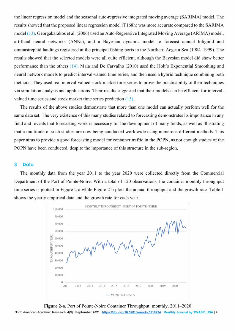
3 Data The monthly data from the year 2011 to the year 2020 were collected directly from the Commercial
Department of the Port of Pointe-Noire. With a total of 120 observations, the container monthly throughput
time series is plotted in Figure 2-a while Figure 2-b plots the annual throughput and the growth rate. Table 1
shows the yearly empirical data and the growth rate for each year.
Figure 2-a. Port of Pointe-Noire Container Throughput, monthly, 2011–2020
0
10,000
20,000
30,000
40,000
50,000
60,000
70,000
80,000
90,000
100,000
2011 2012 2013 2014 2015 2016 2017 2018 2019 2020
THR
OU
GH
PUT
(TEU
)
MONTHLY THROUGHPUT - PORT OF POINTE-NOIRE
MONTHLY DATA

North American Academic Research, 4(9) | September 2021 | https://doi.org/10.5281/zenodo.5516224 Monthly Journal by TWASP, USA | 5
Measure: TEU (Twenty-foot Equivalent Unit)
Figure 2-b. Port of Pointe-Noire Container Annual Throughput and Growth Rate, 2011–2020
Measure: TEU (Twenty-foot Equivalent Unit)
Figure 2-a shows that from 2014 to 2016, the traffic had decreased slightly; then from 2017, it started to
increase again. This can be explained by the collapse in oil prices during the year 2014, leading the country to
a recession, as the country’s economy, due to the lack of diversification, relies mainly on petroleum exports
(16). It is also relevant to note that the World Bank reported that between 2014 and 2016, the Republic of
Congo’s economic complexity index (ECI) deteriorated significantly, from −0.924 to −1.49. Figure 2-b shows
the instability of the growth rate over this decade. It increased from 2011 to 2012, then constantly decreased
from 2012 to 2015, then increased till 2019 before decreasing again in 2020. This instability is due to many
factors, such as the lack of port efficiency, the volatility of the prices of raw materials, or, in the case of the year
2020, the impact of the COVID-19 pandemic.
4 Methodology To conduct this study, a Box–Jenkins ARIMA model was designed.
4.1 Introduction to the model The model was first introduced by George Box and Gwilym Jenkins (17), both British statisticians, for
forecasting time series. The acronym ARIMA stands for Auto-Regressive (AR) Integrated (I) Moving Average
(MA). The model aims to describe autocorrelations in data, and the past values are used to obtain the forecast
values. Each component of the ARIMA model is specified by a parameter, so we have ARIMA (p,d,q), where
p is the parameter for AR, representing the lag order (number of lag observations); d is the parameter for I,
0%
14.76%
12.66%
8.00%
-7.71%
-1.57%
6.63%
23.11%24.59%
0.82%
-10.00%
-5.00%
0.00%
5.00%
10.00%
15.00%
20.00%
25.00%
30.00%
0
100,000
200,000
300,000
400,000
500,000
600,000
700,000
800,000
900,000
1,000,000
2011 2012 2013 2014 2015 2016 2017 2018 2019 2020
CO
NTA
INER
TH
RO
UG
HPU
T (T
EU)
ANNUAL CONTAINER THROUGHPUT OF THE PORT OF POINTE-NOIRE + GROWTH RATE
ANNUAL THROUGHPUT GROWTH RATE

North American Academic Research, 4(9) | September 2021 | https://doi.org/10.5281/zenodo.5516224 Monthly Journal by TWASP, USA | 6
representing the degree of differencing (the number of times actual series observations are differenced in order
to make the series stationary); and q is the parameter for MA, representing the order of the moving average
model (number of lagged prediction errors in the forecast equation). Basically, the ARIMA model is used as a
non-stationary model; this explains the inclusion of I. When the series is already stationary at the beginning,
there is no use in differencing, then d = 0, which gives us ARIMA (p, 0, q), which is equal to ARMA (p, q).
The ARMA (p, q) model with a forecast value of y at time t is given by Eq.(1):
𝑦#$ = 𝑐 +𝜑)𝑦$*) +⋯+ 𝜑,𝑦$*, + 𝛼$ − 𝜃)𝛼$*) −⋯− 𝜃0𝛼$*0 (1)
where 𝑦#$ is the forecast value at period t, 𝑦$*) is the forecast value of the previous period (t−1), 𝑐 is the
constant, 𝜑1 is the coefficient of AR at lag p to be estimated, 𝜃1 is the coefficient of MA at lag p to be estimated
and 𝛼$*1 = 𝑦$*1 − 𝑦#$*1 is the forecast error at time t−p (𝛼′s are a series of residuals, white noise).
Please note that the MA terms in this model are written with a negative sign, in accordance with Box and
Jenkins’ original work.
The ARIMA (p, d, q) model is obtained when the standard ARMA (p, q) model is combined with a
differential process (18). It can be expressed as follows in Eq.(2):
∆5𝑦#$ = 𝑐 + 𝜑)∆5𝑦$*) +⋯+ 𝜑,∆5𝑦$*, + 𝛼$ − 𝜃)𝛼$*) −⋯− 𝜃0𝛼$*0 (2)
where ∆ is the differencing operator and ∆5𝑦#$ is the new series, differenced d times.
A simpler form of the ARIMA structure using the Box–Jenkins backshift operator can be written as follows:
𝜑1(𝐵)(1 − 𝐵)5𝑦#$ = 𝜃0(𝐵)𝛼$ (3)
where (1 − 𝐵) = ∆ (backshift operator).
4.2 Model construction and validation The ARIMA (p, d, q) model consists of three phases:
- Phase 1: Identification of the model
- Phase 2: Estimation and diagnostic checking of the model

North American Academic Research, 4(9) | September 2021 | https://doi.org/10.5281/zenodo.5516224 Monthly Journal by TWASP, USA | 7
- Phase 3: Forecasting
To evaluate the forecasting accuracy, we considered three indexes: MAPE (Mean Absolute Percentage
Error), RMSE (Root Mean Square Error), and MAE/MAD (Mean Absolute Error/Mean Absolute Deviation).
They are expressed as follows:
𝑀𝐴𝑃𝐸 = ∑ ?@ABCA@A
?DAEF
G× 100 (4)
𝑅𝑀𝑆𝐸 =L∑ (MA*NA)ODAEF
G (5)
𝑀𝐴𝐷/𝑀𝐴𝐸 =∑ |MA*NA|DAEF
G (6)
where 𝐴$ is the actual value at time t; 𝐹$ is the forecast value of period (t), and 𝑛is the number of observations.
We used the EViews economic software to construct the ARIMA (p, d, q) model. The time series is named
“THROUGHPUT.”
5 Results
5.1 Identification of the model The stationarity of the time series is first checked. From Figure 2, we can suspect at first sight of the graph
pattern that the data are non-stationary, in which case the use of the ARIMA model may be efficient. To confirm
this suspicion, the correlogram (Figure 3) and a standard unit root test named the Augmented Dickey–Fuller
(ADF) test (Figure 4) are run. As monthly data over 10 years are used, up to 24 lags are selected to conduct the
tests.
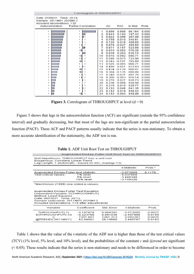
The plot of the correlogram is shown in Figure 3:
North American Academic Research, 4(9) | September 2021 | https://doi.org/10.5281/zenodo.5516224 Monthly Journal by TWASP, USA | 8
Figure 3. Correlogram of THROUGHPUT at level (d = 0)
Figure 3 shows that lags in the autocorrelation function (ACF) are significant (outside the 95% confidence
interval) and gradually decreasing, but that most of the lags are non-significant at the partial autocorrelation
function (PACF). These ACF and PACF patterns usually indicate that the series is non-stationary. To obtain a
more accurate identification of the stationarity, the ADF test is run.
Table 1. ADF Unit Root Test on THROUGHPUT
Table 1 shows that the value of the t-statistic of the ADF test is higher than those of the test critical values
(TCV) (1% level, 5% level, and 10% level), and the probabilities of the constant c and @trend are significant
(< 0.05). These results indicate that the series is non-stationary and needs to be differenced in order to become
North American Academic Research, 4(9) | September 2021 | https://doi.org/10.5281/zenodo.5516224 Monthly Journal by TWASP, USA | 9
stationary.
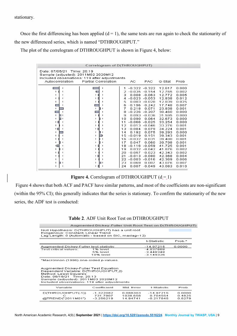
Once the first differencing has been applied (d = 1), the same tests are run again to check the stationarity of
the new differenced series, which is named “DTHROUGHPUT.”
The plot of the correlogram of DTHROUGHPUT is shown in Figure 4, below:
Figure 4. Correlogram of DTHROUGHPUT (d = 1)
Figure 4 shows that both ACF and PACF have similar patterns, and most of the coefficients are non-significant
(within the 95% CI); this generally indicates that the series is stationary. To confirm the stationarity of the new
series, the ADF test is conducted:
Table 2. ADF Unit Root Test on DTHROUGHPUT

North American Academic Research, 4(9) | September 2021 | https://doi.org/10.5281/zenodo.5516224 Monthly Journal by TWASP, USA | 10
From Table 2, it appears that the t-statistic value of the ADF test is greater than those of the TCV and that
the p-values of the constant c and @trend are non-significant (> 0.05). The results of the ADF test show that
the series became stationary after the first differencing.
Once the time series has become stationary, we proceeded by identifying the significant lags at the ACF to
determine q and the PACF to determine p. Figure 5 shows that for ACF, lag 1, lag 6, lag 7, lag 8, and lag 14 are
significant and for PACF, lag 1, lag 6, and lag 8 are significant. This means that q can be 1, 6, 7, or 8 and p can
be 1, 6, or 8. Table 3 shows the possible combinations of p and q to form an ARIMA model we can get from
Figure 5:
Table 3. Possible models combinations of p and q
q
p
1 6 7 8 14
1 (1,1) (1,6) (1,7) (1,8) (1,14) 6 (6,1) (6,6) (6,7) (6,8) (6,14) 8 (8,1) (8,6) (8,7) (8,8) (8,14)
To select the best model from the combinations of models above, they are compared using these criteria:
smallest volatility (SIGMASQ), smallest Akaike Info Criterion (ACI), smallest Hannan–Quinn Information
criterion (HQIC), smallest Schwarz Criterion (SC), most significant coefficients, and the highest R-squared and
Adjusted R-squared. Moreover, it is important to notice that in time series modeling, the well-known principle
of parsimony should also be taken into consideration. This suggests the use of as few parameters as possible;
the simpler the model, the better it is, at least when it produces good results. Over-parameterized models are to
be avoided when possible. This reasoning added to the model comparison leads us to select p = 1 and q = 1,
which gives us an ARIMA (1, 1, 1), as this model gave the best results during the comparison.
5.2 Estimation and diagnostic checking of the model The ARIMA (1, 1, 1) is estimated using the Least Squares (LS) method, and the results are as follows:
Figure 5. Equation estimation of the model
Table 4. ARIMA (1,1,1) equation estimation results

North American Academic Research, 4(9) | September 2021 | https://doi.org/10.5281/zenodo.5516224 Monthly Journal by TWASP, USA | 11
To make sure that the model is good, the correlogram of residuals (CR) and the correlogram of residuals
squared (CRS), also known as the Ljung–Box statistical test, are performed.
Figure 6. Correlogram of residuals
North American Academic Research, 4(9) | September 2021 | https://doi.org/10.5281/zenodo.5516224 Monthly Journal by TWASP, USA | 12
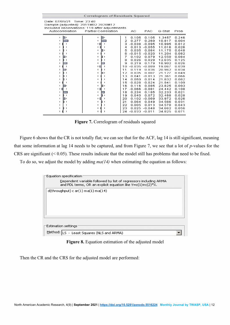
Figure 7. Correlogram of residuals squared
Figure 6 shows that the CR is not totally flat; we can see that for the ACF, lag 14 is still significant, meaning
that some information at lag 14 needs to be captured, and from Figure 7, we see that a lot of p-values for the
CRS are significant (< 0.05). These results indicate that the model still has problems that need to be fixed.
To do so, we adjust the model by adding ma(14) when estimating the equation as follows:
Figure 8. Equation estimation of the adjusted model
Then the CR and the CRS for the adjusted model are performed:

North American Academic Research, 4(9) | September 2021 | https://doi.org/10.5281/zenodo.5516224 Monthly Journal by TWASP, USA | 13
Figure 9. Correlogram of residuals of the adjusted model
Figure 9 shows that the CR is now totally flat; the residuals are white noise, and all the information has been
well captured. The model should be good. To confirm that the adjusted model is good, the Ljung–Box statistical
test is also performed:
Figure 10. Correlogram of residuals squared of the adjusted model
We can see from Figure 10 that all the p-values are now non-significant (> 5%), which indicates good results.
This proves that the adjusted model is good and can be used for forecasting.

North American Academic Research, 4(9) | September 2021 | https://doi.org/10.5281/zenodo.5516224 Monthly Journal by TWASP, USA | 14
5.3 Forecasting
The adjusted ARIMA model is used to forecast the data set.
Figure 11. Forecast results for the adjusted ARIMA Model
Table 5 shows the results of the accuracy indexes for the adjusted ARIMA model.
Table 5. Accuracy measures for the adjusted ARIMA model
Evaluation statistics
Model RMSE MAE MAPE
Adjusted ARIMA
model
5198.920 4030.039 7.713
It can be seen from Figure 11 that the forecasted values fit quite well the actual values of the original time
series. This shows that the adjusted ARIMA model generated good forecast results. Table 5 shows a fairly low
value of MAPE, which generally indicates that the model did well. Seeing high values of RMSE and MAE
should not make us doubt the accuracy of the model, as both have the same units as the dependent variable,
which are large numbers in our data set.
These results prove that the model is good and can be used to forecast the container throughput for the year
2021. Figure 12 plots the graph of the monthly forecasted throughput of the year 2021 whereas Table 6 presents
its annual total throughput.
0
10,000
20,000
30,000
40,000
50,000
60,000
70,000
80,000
90,000
100,000
2011 2012 2013 2014 2015 2016 2017 2018 2019 2020
TH
RO
UG
HPU
T (T
EU
)CONTAINER THROUGHPUT FORECASTING - PORT OF POINTE-NOIRE
ACTUAL VALUES FORECASTED VALUES

North American Academic Research, 4(9) | September 2021 | https://doi.org/10.5281/zenodo.5516224 Monthly Journal by TWASP, USA | 15
Figure 12. Forecasted throughput for the year 2021
Table 6. Forecasting the Port of Pointe-Noire’s throughput for the year 2021 using the adjusted ARIMA
model
Period Throughput (TEU)
Total throughput of 2021 957,500
Figure 12 shows how the throughput is likely to increase in 2021. Table 6 indicates that the total annual
throughput of the POPN is expected to reach 957,000 TEUs in 2021, with a slight growth rate of +3.17% from
2020, where the annual throughput reached 928,124 TEUs. This weak growth rate, which has been observed
since 2020, can be explained by the minor impact of the COVID-19 pandemic on maritime shipping in the
Central Africa sub-region.
6 Conclusion In this study, an adjusted ARIMA model is designed to predict the container traffic of the POPN in the
Republic of Congo. The port is briefly presented, and the model is introduced, built, tested and then used to
forecast the traffic for the year 2021 on the basis of the monthly historical data from 2011 to 2020 (120
observations). The adjusted ARIMA model fit the actual data quite well, showing that it can be used to forecast
future values of container throughput.
By the end of the year 2021, the port container throughput is expected to reach 957,000 TEUs, with a low
growth rate of only +3.17% due to the COVID-19 pandemic. Seeing the general trend of the forecast and
knowing that the export/import demand is likely to increase the more the pandemic is stemmed over time,
solutions must be found in order to avoid any logistical issues in the future.
76,747
77,793
78,431
78,91379,336
79,73580,126
80,51380,899
81,28481,669
82,054
75,000
76,000
77,000
78,000
79,000
80,000
81,000
82,000
83,000
Jan-21 Feb-21 Mar-21 Apr-21 May-21 Jun-21 Jul-21 Aug-21 Sep-21 Oct-21 Nov-21 Dec-21
THR
OU
GH
PUT
(TEU
)
THROUGHPUT FOR YEAR 2021
FORECASTED VALUES

North American Academic Research, 4(9) | September 2021 | https://doi.org/10.5281/zenodo.5516224 Monthly Journal by TWASP, USA | 16
As there is a lack of research papers related to the container traffic forecasting in Central Africa main ports
in general and in the Republic of Congo in particular, this paper represents an important contribution toward
filling this gap. Furthermore, the findings of this study, by providing a trustworthy model, may help the local
authorities to get prepared and develop new strategies and management policies to improve the sustainability
of the port infrastructure.
This study produced good results. However, the scope of this paper only covered the container traffic forecast
based on historical data. Further studies may consider more inputs, such the evolution of the Gross Domestic
Product (GDP) through the years.
References
1. Schweikert A. Republic of the Congo, Port of Pointe Noire [Internet]. The Logistics Capacity Assesment;
2017. Available from:
https://dlca.logcluster.org/display/public/DLCA/2.1.1+Republic+of+the+Congo+Port+of+Pointe+Noire
2. Congo Terminal, Bolloré Ports. Congo Terminal receptionne deux nouveaux portiques de parc [Internet].
Bolloré Transport & Logistics; 2021. Available from: https://congo-
terminal.net//reception_deux_nouveaux_rtg.html
3. Bhalat S. Port de Pointe-Noire, Porte Océane De L’Afrique Centrale 1939-2019 : Historique,
développement et perspectives à l’horizon 2035. Port Autonome De Pointe Noire; 2019.
4. Chen S-H, Chen J-N. Forecasting container throughputs at ports using genetic programming. Expert
Systems with Applications [Internet]. 2010 Mar 15;37(3):2054–8. Available from:
http://www.sciencedirect.com/science/article/pii/S095741740900640X
5. Talluri K, Van Ryzin G. The Theory and Practice of Revenue Management. Springer US; 2004. 713 p.
(International Series in Operations Research & Management Science; vol. 68).
6. Xie G, Zhang N, Wang S. Data characteristic analysis and model selection for container throughput
forecasting within a decomposition-ensemble methodology. Transportation Research Part E: Logistics and
Transportation Review [Internet]. 2017 December;108:160–78. Available from:
http://www.sciencedirect.com/science/article/pii/S1366554517300455
7. Dragan D, Kramberger T. Forecasting the Container Throughput in the Port of Koper using Time Series
ARIMA model. In Celje, Slovenia; 2014. Available from:
https://www.researchgate.net/publication/333974184_Forecasting_the_Container_Throughput_in_the_P
ort_of_Koper_using_Time_Series_ARIMA_model/link/5d10bc7f458515c11cf308d3/download
North American Academic Research, 4(9) | September 2021 | https://doi.org/10.5281/zenodo.5516224 Monthly Journal by TWASP, USA | 17
8. Chen Z, Chen Y, Li T. Port Cargo Throughput Forecasting Based On Combination Model. In: 2016 Joint
International Information Technology, Mechanical and Electronic Engineering Conference [Internet].
Atlantis Press; 2016. Available from: https://doi.org/10.2991/jimec-16.2016.25
9. Chen J. Research on Container Sea-Rail Intermodal Transport in Qingdao Port Based on Volume Forecast
and Benefit Analysis [Internet]. Ocean University Of China; 2013. Available from:
https://wenku.baidu.com/view/9b606f5f2f60ddccda38a0a8.html
10. Wu H, Liu G. Container Sea-Rail Transport Volume Forecasting of Ningbo Port Based on Combination
Forecasting Model. In: International Conference on Advances in Energy, Environment and Chemical
Engineering [Internet]. Atlantis Press; 2015. Available from: https://doi.org/10.2991/aeece-15.2015.91
11. Gamassa P, Chen Y. Application of Several Models for the Forecasting of the Container Throughput of
the Abidjan Port in Ivory Coast. International Journal of Engineering Research in Africa. 2017 Jan
1;28:157–68.
12. Seabrooke W, Hui ECM, Lam WHK, Wong GKC. Forecasting cargo growth and regional role of the port
of Hong Kong. Cities [Internet]. 2003 Feb 1;20(1):51–64. Available from:
http://www.sciencedirect.com/science/article/pii/S0264275102000975
13. Fang T, Lahdelma R. Evaluation of a multiple linear regression model and SARIMA model in forecasting
heat demand for district heating system. Applied Energy [Internet]. 2016 Oct 1;179:544–52. Available
from: http://www.sciencedirect.com/science/article/pii/S0306261916309217
14. Georgakarakos S, Koutsoubas D, Valavanis V. Time series analysis and forecasting techniques applied on
loliginid and ommastrephid landings in Greek waters. Fisheries Research [Internet]. 2006 Apr 1;78(1):55–
71. Available from: http://www.sciencedirect.com/science/article/pii/S0165783605003292
15. Maia ALS, de Carvalho F de AT. Holt’s exponential smoothing and neural network models for forecasting
interval-valued time series. International Journal of Forecasting [Internet]. 2011 Jul 1;27(3):740–59.
Available from: http://www.sciencedirect.com/science/article/pii/S0169207010000506
16. Husted TF, Arieff A. The Republic of Congo (Congo-Brazzaville) [Internet]. Library of Congress.
Congressional Research Service; 2019 Sep. Report No.: CRS In Focus, IF11301. Available from:
https://www.hsdl.org/?view&did=829483
17. Box GEP, Jenkins GMJ. Time Series Analysis: Forecasting and Control. San Francisco: Holden-Day;
1970.

North American Academic Research, 4(9) | September 2021 | https://doi.org/10.5281/zenodo.5516224 Monthly Journal by TWASP, USA | 18
18. Box GEP, Jenkins GMJ, Reinsel GC, Ljung GM. Time Series Analysis: Forecasting and Control. 5th
Edition. New-York: John Wiley and Sons; 2015. 712 p.
© 2021 by the authors. Author/authors are fully responsible for the text, figure,
data in above pages. This article is an open access article distributed under
the terms and conditions of the Creative Commons Attribution (CC BY) license
(http://creativecommons.org/licenses/by/4.0/)