Forecasting Empty Container Volumes

217

The Asian Journal of Shipping and Logistics Volume 27 Number 2 August 2011 pp 217-236

Forecasting Empty Container Volumes

Rafael DIAZ Wayne TALLEY Mandar TULPULE

Contents

I Introduction II Literature Review Repositioning Empty ContainersIII Literature Review Forecasting Empty Container Volumes at Ports IV Forecasting Empty Container Volumes Empirical Analysis V Conclusion

Abstract

The accumulation and repositioning of empty containers have become acute problems for container ports and are expected to intensify in the future given the expected growth in trade imbalances among trading nations These problems are major costs and operational challenges for container ports More accurate forecasting of volumes of port empty containers will enable container ports to develop more cost efficient plans for the repositioning of empty containers This paper compares the Tioga Group United Nations and Winters method (utilizing empty container volumes of three US container ports) in forecasting volumes of port empty containers The Winters method is found to provide more accurate forecasts of volumes of port empty containers than the Tioga Group and United Nations methods

Key words Empty Containers Forecasting Winters method Research Assistant Professor of Old Dominion University USA Email rdiazoduedu Professor of Old Dominion University USA Email wktalleoduedu Research Assistant of Old Dominion University USA Email mtulp001oduedu

218


I Introduction

The use of ocean containers in marine transportation has steadily increased since their introduction about half a century ago The growth in container trade has been enhanced in recent years by the economic development in Asia particularly in China Worldwide ocean container traffic increased from 846 million TEUs (Twenty-foot equivalent units) in 1990 to 362 million TEUs in 20051) The annual growth rate in container traffic has been 102 in comparison to the 6 growth rate in world trade2) For US ports container traffic increased from 155 million TEUs in 1990 to 45 million TEUs in 20073)

Imbalance in global trade is the fundamental cause for the imbalance in the supply of and demand for empty containers and thus the repositioning of empty containers among ports4) For example the Europe-Asia trade route has more containers with export cargo from Asia to Europe than from Europe to Asia Consequently there are fewer containers being returned to Asia from Europe Thus European ports are experiencing a surplus of empty containers while Asian ports are experiencing a shortage of empty containers Similarly the large trade imbalance between Asia and North America (with Asiarsquos exports to the US exceeding its imports from the US) has also resulted in a significant surplus of empty containers in the US5) Although the US trade imbalance has declined somewhat during the recent global economic recession this trade imbalance is expected to persist in the foreseeable future Thus the problem of repositioning empty containers by shipping lines from surplus empty-container ports to shortage empty-container ports will remain for the foreseeable future

The repositioning of empty containers is not only impacted by the decisions of container ports but also by the decisions of container shipping lines container leasing companies intermodal carriers shippers and other involved parties Ports may influence the repositioning of empty containers

1) Song and Carter (2009)2) Song and Carter (2009)3) American Association of Port Authorities (2009)4) Boile (2006)5) The Tioga Group (2002)

219


by shipping lines through storage tariff changes Since containers are owned by container shipping lines and container leasing companies the decisions of container owners in the repositioning containers may differ depending on their individual policies Shippers in a competitive shipping market may have more choices in obtaining empty containers given that shipping lines in facing competition are expected to reposition empty containers more quickly6) Also the cost of manufacturing new containers primarily driven by the cost of steel7) may influence the repositioning of empty containers ie higher the cost of constructing new containers less the number of new containers that will be constructed and thus an increase in the repositioning of empty existing containers8) Other factors influencing the repositioning of empty containers include the cost of transporting (by sea and intermodal) empty containers the cost of maintenance repair and inspection of containers and the dynamics of the container leasing industry9) Although the importance of more accurate forecasts of empty containers is evident the subject has received little attention in the literature With more accurate forecasts of empty containers ports as well as shipping lines are in position to reduce the cost of repositioning empty containers within port areas and to destination ports The purpose of this paper is to compare and evaluate methods used heretofore and a new method the Winters Method for forecasting empty container volumes at ports Since shipping lines cannot reposition empty containers to destination ports unless they are at origin ports the paper will only evaluate methods for forecasting empty container volumes at origin ports The following section of the paper presents a literature review of strategies for repositioning empty container by shipping lines and ports Section 3 presents a literature review of forecasting empty container volumes at ports Section 4 uses the Winters method and methods used heretofore to forecast empty container volumes at the US container ports of Long Beach Los Angeles and Savannah These forecasts are the basis for the evaluation of the forecasting methods Conclusions follow in Section 5

6) Song and Carter(2009)7) Boile(2006)8) Theofanis and Boile(2009) Boile(2006)9) BoileTheofanis Golias and Mittal(2006)

220


II Literature Review Repositioning Empty Containers

1 Shipping LinesShipping lines use their ships to transport containers (loaded and empty)

over sea transportation networks At destination ports containers containing cargo are unloaded from ships and transported by domestic transportation carriers (truck rail and water) to the destination locations of receivers (or consignees) The empty containers that are returned (by domestic carriers) to the shipping line are placed in a container storage yard in the port or outside of (but near) the port to meet future requests for containers by shippers Alternatively the empty containers that are not placed in container storage yards are used and requested by shipping lines and shippers Containers requested by shippers are loaded at their own premises and returned to the port

If shipping lines do not have enough of their own containers to meet the requests of shippers at a given port they usually turn to container leasing companies to hire enough containers to meet requests10) and then lsquooff leasersquo containers at ports where empty containers are in surplus The majority of containers that are in use worldwide are owned by shipping lines In 2007 59 of containers were owned by shipping lines and the remainder by leasing companies11) The advantages of container ownership by shipping lines include 1) increased visibility of the line to the customer 2) improved equipment inventory management and 3) improved customer service12) An alternative to leasing containers by shipping lines in order to avoid the repositioning of containers is to purchase rather than lease containers in port areas where empty containers are in demand However the decision whether to lease or purchase containers will be based upon their comparative costs Thus in order to meet the requests for empty containers by shippers shipping lines are faced with the challenge of repositioning empty containers from supply ports (where the supply of empty containers is greater than the demand) to demand ports (where the demand for empty containers is greater

10) Shintani Nishimura and Papadimitriou(2007)11) Theofanis and Boile(2009)12) Theofanis and Boile(2009)

221


than the supply) and leasing (purchasing) a minimum number of empty containers from leasing companies (container manufacturers)13)

The repositioning of empty containers provides the shipper the benefit of reduced waiting times to receive empty containers while benefiting the shipping line through increased utilization of containers and the revenue thus received14) Alternatively the shipping line incurs transportation and handling costs for non-revenue-generating (or empty) containers and the opportunity cost of revenue foregone by using space on ships for which revenue-generating containers could have occupied The costs incurred by container shipping lines in repositioning empty containers are significant and thus affect the operating margins of these lines15)

Two criteria have been used by container shipping lines in developing strategies for repositioning empty containers 1) internal coordination ndash coordinating container flows across different service routes and 2) external container sharing ndash pooling (or sharing) containers among shipping lines Empty container repositioning strategies based upon these two criteria include 1) container sharing with route coordination ndash shipping lines sharing containers across all routes 2) container sharing without route coordination ndash shipping lines sharing containers but there is no coordination among routes 3) route coordination without container sharing ndash shipping lines do not share containers but try to balance container flows across their routes and 4) neither route coordination nor container sharing ndash shipping lines try to balance their container flows on individual routes with no coordination among routes and no container sharing among shipping lines16)

2 PortsThe repositioning of empty containers within a port area ie the port

and its adjacent area increases the number of truck trips in the area (likely contributing to the arearsquos highway congestion and air and noise pollution) At the ldquoLos AngelesLong Beach port area a small percentage reduction in

13) Li Leung Wu and Liu(2007)14) Dong Song(2009)15) United Nations(2007)16) Song and Carter(2009)

222


empty repositioning traffic can be reflected in significant congestion reduction and improved operating costsrdquo17) The number of empty containers that are repositioned in a port area can be reduced by reusing these containers in the port area ie using empty import containers for export loads without first returning them to the port The two strategies for doing so include the depot-direct and street-turn strategies

The depot-direct strategy has empty containers being stored maintained and interchanged at off-port container depots that experience less highway congestion than that for the port The street-turn strategy has import containers in the port area that have been unloaded and now are empty containers that have been directly moved to local shippers for the loading of export cargo

III Literature ReviewForecasting Empty Container Volumes at Ports

Since 1998 20 of all containers handled by ports have been empty containers18) A container port in planning for its future container handling capacity would like to know the volume of containers that it is expected to receive in the future Forecasting such volumes is often a requirement of port planning departments19) However there has been little discussion in the literature of the methods used by ports in forecasting future volumes of containers

Ports generally use the statistical regression model for forecasting volumes of containers Such a model expresses a portrsquos volume of containers as a function of international trade growth and various macroeconomic variables20) Ports also use the lsquoshift and sharersquo forecasting model for forecasting container volumes21) The latter model is used to forecast international trade flows by major commodity and then the share of the forecasted trade flows that would potentially be handled by a given port Trade flows are forecasted using trend

17) Jula Chassiakos and Ioannou(2006)18) United Nations(2007)19) Chou Chu and Liang(2008)20) Chou Chu and Liang(2008)21) Dagenais and Martin(1987)

223


analysis and econometric estimations of import and export trade flows for a portrsquos region Studies by22) have used econometric models to forecast the trade growth of a region as a function of its Gross Domestic Product (GDP) population industrial production index agricultural GDP industrial GDP and Service GDP However these studies provide trade growth forecasts and not container volume forecasts

Although determinants of empty container volumes are generally the same as the determinants of non-empty containers trade imbalances among countries are more important factors affecting empty container volumes than non-empty container volumes Greater the trade imbalance for containerized cargo for a given country ie greater the difference between its import and export containerized cargoes greater will be the number of empty containers flowing to andfrom the country and its container ports A study forecasting empty container volumes for the Ports of Long Beach and Los Angeles concluded (using an econometric model) that the outbound empty container volume for the two ports is 88 percent of their total forecasted empty container volume23) (referred to as lsquoTioga methodrsquo henceforth)

Thus if lsquoDt-1rsquo is the actual difference between the total loaded inbound and total loaded outbound containers during the period lsquot-1rsquo then the forecasted outbound empty container volume for period lsquotrsquo represented by lsquoMtrsquo can be expressed as in equation (1) below

Mt = 088 times Dt-1 (1)

A forecast of the worldrsquos volume of empty container flows (or movements) using a simplified approach consisting of two major steps is found in a study by the United Nations (2007) In the first step the study adds 35 to the volumes of non-empty containers in the major flow (importexport) direction for a given port In the second step the empty container volume in the minor direction is then calculated by subtracting the number of loaded containers in the minor flow direction from the newly calculated total volume in the major

22) Dollar(1992) Kavoussi(1984) Ram(1985 1987)23) Study was conducted by the Tioga Group(2007)

224


flow direction (this method is referred to as the lsquoUnited Nations methodrsquo henceforth) Thus if lsquoFMA(t-1)rsquo represents the volume of non-empty containers in the major flow direction and lsquoFMI(t-1)rsquo represents the volume of non-empty containers in the minor flow direction during the period lsquot-1rsquo then the forecasted volume of empty containers lsquoMtrsquo during period lsquotrsquo would be given as below

Mt = 1035 times FMA(t-1) - FMI(t-1) (2)

This study justifies the use of such a simplified approach ndash owing to the minor impact of the imbalances on the overall container volumes and the difficulties in predicting actual empty container ratios The study concludes that empty containers constitute about 20 of container flows worldwide

An alternative method to those of the Tioga Group and the United Nations for forecasting port empty container flows is the Winters method The Winters method uses exponentially weighted moving averages to replicate a time series that has trend and seasonality effects The weights are the time series factors level trend and seasonality symbolized by alpha beta and gamma respectively Any observed demand can be decomposed into a systematic and random component The systematic component measures the expected value of demand and consists of lsquolevelrsquo that represents the current deseasonalized demand lsquotrendrsquo that represents the rate of decline or growth and lsquoseasonalityrsquo that corresponds to the predictable seasonal fluctuation Initial estimates of the level and trend are obtained via a regression analysis of the deseasonalized data The regression equation expresses demand as a function of time For a two dimensional Cartesian coordinate system say (XY) the regression is in the form of a straight line with lsquodemandrsquo plotted on the Y-axis and lsquotimersquo plotted on the X-axis Under this scenario the lsquolevelrsquo represents the intercept of the regression line on the Y-axis and lsquotrendrsquo represents slope of the regression line Thus the lsquolevelrsquo can be thought of as the estimate of demand at time zero while the lsquotrendrsquo gives the rate of increase or decrease in demand for each subsequent period Seasonality factors are calculated by taking the ratio of the deseasonalized data and the original values The estimates of

225


level trend and seasonality are updated with each newly observed data point A discussion of the Winters method follows24) A multiplicative trend-seasonal method may be characterized as follows

( )t t tx a bt F ε= + + (3)

Where tx is the demand in period t a is a level b is a trend tF is a seasonal factor and

tεis assumed to be an independent random variable with

mean 0 and constant variance 2σ though it is not necessary that the error terms be normally distributed The season is assumed to be of length P periods and the seasonal indices are normalized Thus at any point the sum of the indices over an entire season is exactly equal to P iesumt=1

P Ft =P The following procedure to forecast the next periodrsquos demand is suggested25)

1 1ˆˆˆ ˆ( ) (1 )( )t t t P t ta x F a bα αminus minus minus= + minus + (4)

1 1ˆ ˆˆ ˆ( ) (1 )( )t t t tb a a bβ βminus minus= minus + minus (5)

ˆ ˆˆ( ) (1 )( )t t t t PF x a Fγ γ minus= + minus (6)

where α β and γ are smoothing constants with values between 0 and 1 Many authors have established different criteria and procedures to select these smoothing constants26) All procedures fall into two broad categories 1) estimating the smoothing coefficients as decision variables in a minimization problem where the objective function is a function of the forecasting error or 2) simply guessing the appropriate values by judgment27) A simple but reliable method is to test the model at different coefficient values over their range [0 1] to find the set of values that provide the least amount of forecasting error28)

24) The discussion is based on Silver(1985)25) Winter(1960)26) Gardner and Dannengbring(1980)27) Chatfield and Yar(1988)28) This method is equivalent to the method of the smoothing of coefficients by judgment as described by Chatfield and Yar(1988) However the judgment in this case is made on the basis of performing a number of experiments using different coefficient values in order to find the set of values that gives the least forecasting error For a detailed discussion on issues related to coefficient value selection see Chatfield and Yar(1988)

226


This study has used this method for coefficient estimation

The term ˆt t Px F minus in equation (4) is an estimate of the deseasonalized actual demand in period t t PF minus is the value of the seasonal index for the latest equivalent period in the seasonal cycle The difference term 1ˆ ˆt ta a minusminus

in equation (5) is an estimate of the real trend in period t The term ˆt tx a in equation (6) is an estimate of the seasonal factor based on the most recent demand Thus as all fundamental exponential smoothing basic equations reflect these equations mirror a linear combination of the historical information and the estimate is derived from the latest demand information It is desirable to permanently have the sum of the indices through an entire season add to P Accordingly when a particular index is revised all indices are renormalized to achieve this equality The detailed explanation of the method can be found in29) While equation (3) is to be used for ex-post forecasting the equation (7) below is used for ex ante forecasting

xtt+ω =(acirct +bt ω ) Ft+ω-P (7)

Equation (7) gives the forecast (xtt+ω) for a period (t+ω) based on the model in period ( t ) where acirct is the estimate of level at time lsquotrsquo bt is the estimate of trend at time lsquotrsquo and Ft+ω-P is the estimate of the seasonal factor at time lsquot+ω-Prsquo with the constraint that (ω le P ) This constraint is necessary since the forecast is based on the model at time lsquotrsquo and any information beyond lsquotrsquo is unavailable

The difference between a forecasted and an actual parameter is the forecasting error for the parameter Since the basic purpose of a forecasting method is to provide an accurate forecast forecasting error becomes the obvious means for comparing the performance of different forecasting methods The most common statistics used in evaluating the forecasting accuracy of forecasting methods are the Mean Squared Error (MSE) Mean Absolute Deviation (MAD) and Mean Absolute Percentage Deviation (MAPE)

A forecast error for period t may be represented by εt and defined as the

29) Winters(1960)

difference between actual and predicted demand or εt=xt - xt-1t The MSE may be expressed as

2

1

1 n

n tt

MSEn

ε=

= sum (8)

The MSE is the variance of the forecast error The absolute deviation in period t At can be described as the absolute value

of the error in period tAt=|ε t| As a result the mean of absolute deviation over all periods can be described by

(9)

The MAD can be used to estimate the standard deviation of the random component assuming that the random component is normally distributed This is usually defined by σ=125MAD30)

The mean absolute percentage error MAPE is usually represented by the average absolute error as a percentage of demand

(10)

In general the sum of forecast errors can be used to verify whether a forecasting method consistently over or underestimates demand Equation 10 presents this simple characterization

(11)

Overall if the error is truly random the BIAS will oscillate around 0 In this study MAD and MSE are used in evaluating the forecasting performances of the forecasting methods31) MAD is extensively used in the context of

30) Silver(1985)31) A summary discussion on the use and interpretation of the above statistics in a supply chain context is found in Chopra and Meindl(2006)

227


228


inventory control problems32) Empty container repositioning can be broadly defined as an inventory control problem and hence using MAD seems logical The MSE is calculated as the average of the sum of the squares of forecasting errors and is similar to MAD apart from the fact that it is more punitive towards large errors than MAD In the following section the Winters Tioga Group and United Nations methods are used to forecast empty container flows at the US Ports of Long Beach Los Angeles and Savannah It is shown that the Winters Method performs better in forecasting empty container flows at these ports than the Tioga Group and United Nations forecasting methods

IV Forecasting Empty Container Volumes Empirical Analysis

1 Port of Long BeachThe Port of Long Beach (California) is the second largest container port

in the US and is a major US port for receipt of containerized cargo from Asia Over the last decade it has experienced large trade imbalances between imports and exports With the former greatly exceeding the later the port has experienced a heavy outbound flow of empty containers In the year 2009 for example total empty containers handled at the Port of Long Beach were about 4533) of the loaded outbound container traffic at the port34)

In Figure 1 below monthly outbound empty containers for the Port of Long Beach for selected years is found Figure 1 clearly shows a trend and seasonality that is repeated year after year The trend is evident from the steady increase in the volume of empty container flows from 1995 to 2005 The seasonality in the yearly volume of outbound empty containers for each year in Figure 1 is revealed with the dip in this volume in the first quarter of each year followed by a steady rise in the volume over the next two quarters and ending with a dip in the volume in the last half of the fourth quarter

The monthly data of outbound empty containers for the Port of Long Beach for the period 1995-2009 are used to generate ex ante35) monthly forecasts of outbound empty container volumes at the Port of Long Beach by the Winters

32) Armstrong and Callopy(1992)33) This approximate value was calculated based on data found in the Port of Long Beach TEU Stats Archives 2009 Accurate year by year values are found in the Port of Long Beach TEU Stats Archives(2009)34) Port of Long Beach TEU Stats Archives(2009)35) The term ldquoex-anterdquo means ldquoexpected before the eventrdquo It is commonly employed in settings where results are predicted in advance Conversely the term ex-post means ldquoafter the event or actualrdquo

Tioga Group and United Nations methods The ex ante forecasts are generated by fitting these methods to the data and then using the methodsrsquo fitted equations to forecast the monthly volume of empty containers for each month for the time period 1995 ndash 2009 The smoothing coefficients α β and γ for the Winters method are estimated by numerous systematic experiments within the range of α β and γ to 075 0 and 01 respectively Extensive preliminary experimentation was conducted to ensure that these values correspond to the least values for MAD and MSE and thus represent the best performing method for the given data

lt Figure 1 gt Monthly volume of outbound empty containers in TEUs for the Port of Long Beach for selected years36)

The forecasted volume of empty containers for each month is compared to the actual volume for that month The difference between the monthly forecasted volume and the monthly actual volume of empty containers is the forecast error Forecast errors are then used to calculate the MSE and MAD statistics for the three forecasting methods The ex ante forecasting ability of the three methods is evaluated using the calculated MSEs and the MADs

Figure 2 plots the actual and forecasted monthly volumes of empty containers for all months for the years 1995-2009 based upon the three forecasting methods The method for which its forecasted volumes are nearest the actual volumes of empty containers will be referred to as the best

36) Port of Long Beach TEU Stats Archives(2009)

229


forecasting method among the three methods Visually it can be seen that the Winters plot of forecasted empty containers fits the actual empty containers better than the other two methods This is borne out by the evidence found in Table 1 where the MADs and MSEs for the three forecasting methods are found The Winters method has substantially lower values for MAD and MSE and thus forecasting errors than those of the Tioga Group and United Nations methods

ltFigure 2gt Forecasted and actual volumes of outbound empty containers for the Port of Long Beach (monthly values for the years 1995-2009)37)

ltTable 1gt The Mean Squared Error and the Mean Average Deviation for Forecasting Methods for the Port of Long Beach

Tioga Group United Nations Winters

MSE 3778076288 7628445076 1106918762

MAD 1538881 2280004 809258

2 The Port of Los AngelesThe Port of Los Angeles (California) is the largest container port in the

US and like the Port of Long Beach is a major US port for receipt of

37) The Port of Long Beach TEU Stats Archives(2009)

230


containerized cargo from Asia In 2009 the Port of Los Angelesrsquo volume of outbound empty containers were about 4538) of the total outbound volume of containers at the port Figure 3 plots the actual and forecasted monthly volumes of empty containers for the Port of Los Angeles for the years 1995-2009 Forecasts from all three forecasting methods are presented The MADs and MSEs for the three forecasting methods are found are found in Table 2 As for the Port of Long Beach the Winters method performed substantially better in forecasting the volume of empty containers than the other two forecasting methods

ltFigure 3gt Forecasted and actual monthly volumes of outbound empty containers for the Port of Los Angeles (All months from 1995-2009)39)

The smoothing coefficients α β γ for the Winters method are 04 0 06 respectively The interpretations of the coefficients are similar to those for the Port of Long Beach However for the Port of Angeles the value of α=04 indicates that the near term estimates of level are less indicative of the current estimates of the level for the Port of Los Angeles as compared to the Port of Long Beach

38) Approximate value calculated for demonstration purpose on the basis of data from Port of Los AngelesStatistics (2009) For accurate year by year values refer to data from Port of Los Angeles Statistics(2009)39) Port of Los Angeles Statistics(2009)

231


232


ltTable 2gt The Mean Squared Error and the Mean Average Deviation for Forecasting Methods for Los Angeles California


MSE 48452595741 206842959739 17840319547

MAD 1538689 3713917 1002573

3 Port of Savannah GeorgiaThe Port of Savannah is the fourth largest container port in the US and

the second largest container port on the US East Coast The volume of trade between exports and imports at the Port of Savannah is quite balanced However the volume of outbound empty containers has been consistently higher than the volume of inbound empty containers As for the Ports of Long Beach and Los Angeles the Winters method performs better than the Tioga Group and the United Nations methods in forecasting the monthly volumes of empty containers at the Port of Savannah This is evident from the actual and forecasted monthly volumes of outbound containers in Figure 4 and the MSE and MAD values found in Table 3

ltFigure 4 gt Forecasted and actual monthly volumes of outbound empty containers for the Port of Savannah (All months from 2003-2009)40)

40) Port of Savannah Sales and Marketing(2009)

233


ltTable 3gt The Mean Squared Error and the Mean Average Deviation for Forecasting methods for Savannah Georgia


MSE 43348867899 49264815961 4167525962

MAD 1892757 2093107 493331

The smoothing coefficients α β and γ for the Port of Savannah are 07 0 and 05 respectively These values agree in principle with the values estimated for the Port of Los Angeles and the Port of Long Beach Thus the same interpretation for the Winters method for the Port of Savannah is similar to the interpretations for the Winters method for the Ports of Long Beach and Los Angeles

V Conclusion

This paper has evaluated the Winters Tioga Group and United Nations methods for forecasting empty container volumes at container ports Among these three methods only the Tioga Group method has been used in the past to forecast volumes of port empty containers The forecasting abilities of the three methods were evaluated using the statistics MAD (Mean Absolute Deviation) and MSE (Mean Squared Error) whose values are based upon the forecasting errors in forecasting empty container volumes for the US container ports ndash Port of Long Beach Ports of Los Angeles and Port of Savannah The evaluations found that the Winters method is a more accurate forecaster of empty container volumes than the Tioga Group and United nations methods Further the smoothing coefficients for the Winters method for all the three ports indicate that the levels of empty container volumes are best estimated by their levels in the nearest past period However the nearest past period is not a good indicator of the expected trend This inference seems logical from looking at the high volatility in the empty container volumes

In forecasting empty container volumes the Tioga Group and United Nations methods express the volume of empty containers as a function of

234


the trade imbalance ie the difference between imports and the exports Trade imbalance has been cited as the most dominant factor contributing to a portrsquos volume of empty containers However the general assumption of a positive relationship between a portrsquos trade imbalance and its volume of empty containers may not be universally applicable For example the Port of Savannah has a high outbound volume of empty containers even though the volume of container trade for Savannah is relatively balanced ie the difference between the export and import TEUs is relatively low Future research should investigate whether the Winters method or an alternative method is universally a more accurate forecaster of volumes of empty containers at container ports

Date of Contribution Dec 4 2010 Date of Acceptance August 5 2011

235


References

AMERICAN ASSOCIATION OF PORT AUTHORITIES(2009) Port Industry StatisticsNorth American Port Container Traffic 1990-2009 Retrieved September 20 2010 from wwwaapaorg httpwwwaapa-portsorgIndustrycontentcfmItemNumber=900ampnavItemNumber=551

ARMSTRONG J S AND CALLOPY F (1992) ldquoError Measures for Generalizing About Forecasting Methods Empirical Comparisonsrdquo International Journal of Forecasting Vol 8 pp69-80

BOILE M (2006) Empty intermodal container management Rutgers University Center for Advanced Infrastructure and Trasportation

BOILE M THEOFANIS S GOLIAS M AND MITTAL N (2006) ldquoEmpty marine container management- Addressing locally a global problemrdquo InProceedings of 85th Annual Meeting of the Transportation Research Board

CHATFIELD C AND YAR M (1988) ldquoHolt-Winters Forecasting Some Practical Issuesrdquo Journal of the Royal Statistical Society Vol 37 No 2 pp129-140

CHOPRA S AND MEINDL P (2006) Supply Chain Management Strategy Planning and Operation Prentice Hall

CHOU C C CHU C W AND LIANG G S (2008) ldquoA modified regression method for forecasting the volumes of Taiwanrsquos import containersrdquo Mathematical and Computer Modelling Vol 47 No 9-10 pp797-807

DAGENAIS M G AND MARTIN F (1987) ldquoForecasting containerized traffic for the port of Montreal (1981-1995)rdquo Transportation Research Part A Vol 21 No1 pp1-16

DOLLAR D (1992) ldquoOutward-oriented developing economies really do grow more rapidlyEvidence from 95 LDCs1976-1985rdquo Economic Development and Cultural Change Vol40 No3 pp523-544

DONG J X AND SONG D P (2009) ldquoContainer Fleet Sizing and Empty Repositioning in Liner Shipping Systemsrdquo Transportation Research Part E Vol 45 pp860-877

GARDNER E S AND DANNENGBRING D G (1980) ldquoForecasting with exponential smoothing Some guidelines for model selectionrdquo Decision Science Vol 11 No 2 pp370-383

JULA H A CHASSIAKOS A AND IOANNOU P (2006) ldquoPort Dynamic Empty Container Reuserdquo Transportation Research Part E Vol 42 pp43-60

KAVOUSSI R M (1984) ldquoExports expansion and economic growth further empirical evidencerdquo Journal of Development Economics Vol 14 No 1 pp241-250

236


LI J A LEUNG S H WU Y AND LIU K (2007) ldquoAllocation of Empty Containers Between Multi-Portsrdquo European Journal of Operational Research Vol 182 pp400-412

PORT OF LONG BEACHTEU STATS ARCHIVES (2009) Retrieved from httpwwwpolbcomeconomicsstatsteus_archiveasp

PORT OF LOS ANGELES STATISTICS (2009) Retrieved from httpwwwportoflosangelesorgmaritimestatsasp

PORT OF SAVANNAH SALES AND MARKETING (2009) Retrieved from httpwwwgaportscomSalesandMarketingMarketingBusinessDevelopmentGPABytheNumberstabid435Defaultaspx

RAM R (1987) ldquoExports and economic growth in developing countries Evidence from time-series and cross-section datardquo Economic Development and Cultural Change Vol 36 No 1 pp51-72

RAM R (1985) ldquoExports and economic growth Some additional evidencerdquo Economic Development and Cultural Change Vol 33 No 2 pp415-425

SHINTANI K A NISHIMURA E AND PAPADIMITRIOU S (2007) ldquoThe Container Shipping Network Design Problem with Empty Container Repositioningrdquo Transportation Research Part E Vol 43 pp39-59

SILVER E (1985) Decision Systems for Inventory Management and Production Planning New York Wiley

SONG D P AND CARTER J (2009) ldquoEmpty Container Repositioning in Liner Shippingrdquo Maritime Policy and Management Vol 36 pp291-307

THE TIOGA GROUP (2002) Empty Ocean Logistics StudyTechnical Report Submitted to the Gateway Cities Council of Governments CA

THE TIOGA GROUP (2007) San Pedro Bay Cargo Forecast Draft Report Prepared for the Ports of Los Angeles and Long Beach

THEOFANIS S AND BOILE M (2009) ldquoEmpty marine container logistics facts issues and management strategiesrdquo GeoJournal Vol 74 No 1 pp51-65

UNITED NATIONS ECONOMIC AND SOCIAL COMMISSION FOR ASIA AND THE PACIFIC (2007) Regional Shipping and Port Development Container Traffic Forecast Update 2007

WINTERS P R (1960) ldquoForecasting Sales by Exponentially Weighted Moving Averagesrdquo Management Science Vol 6 No 3 pp324-342

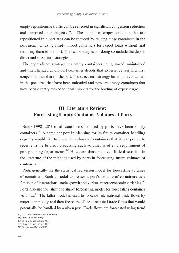
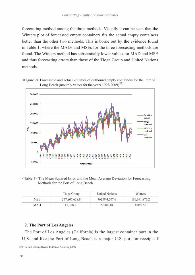
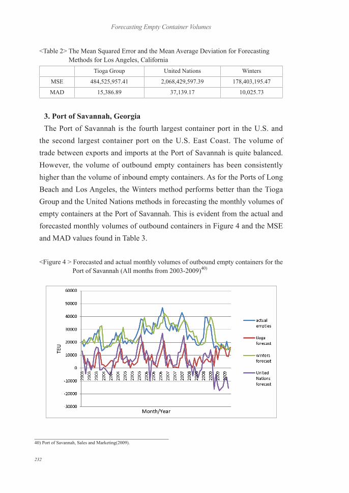218


I Introduction

The use of ocean containers in marine transportation has steadily increased since their introduction about half a century ago The growth in container trade has been enhanced in recent years by the economic development in Asia particularly in China Worldwide ocean container traffic increased from 846 million TEUs (Twenty-foot equivalent units) in 1990 to 362 million TEUs in 20051) The annual growth rate in container traffic has been 102 in comparison to the 6 growth rate in world trade2) For US ports container traffic increased from 155 million TEUs in 1990 to 45 million TEUs in 20073)

Imbalance in global trade is the fundamental cause for the imbalance in the supply of and demand for empty containers and thus the repositioning of empty containers among ports4) For example the Europe-Asia trade route has more containers with export cargo from Asia to Europe than from Europe to Asia Consequently there are fewer containers being returned to Asia from Europe Thus European ports are experiencing a surplus of empty containers while Asian ports are experiencing a shortage of empty containers Similarly the large trade imbalance between Asia and North America (with Asiarsquos exports to the US exceeding its imports from the US) has also resulted in a significant surplus of empty containers in the US5) Although the US trade imbalance has declined somewhat during the recent global economic recession this trade imbalance is expected to persist in the foreseeable future Thus the problem of repositioning empty containers by shipping lines from surplus empty-container ports to shortage empty-container ports will remain for the foreseeable future

The repositioning of empty containers is not only impacted by the decisions of container ports but also by the decisions of container shipping lines container leasing companies intermodal carriers shippers and other involved parties Ports may influence the repositioning of empty containers

1) Song and Carter (2009)2) Song and Carter (2009)3) American Association of Port Authorities (2009)4) Boile (2006)5) The Tioga Group (2002)

219




220







221








222








223





Mt = 088 times Dt-1 (1)



224






225



( )t t tx a bt F ε= + + (3)










226









29) Winters(1960)


2

1

1 n

n tt

MSEn

ε=

= sum (8)



(9)



(10)


(11)



227


228














229






MSE 3778076288 7628445076 1106918762

MAD 1538881 2280004 809258




230






231


232




MSE 48452595741 206842959739 17840319547

MAD 1538689 3713917 1002573





233




MSE 43348867899 49264815961 4167525962

MAD 1892757 2093107 493331


V Conclusion



234




235


References














236
















219




220







221








222








223





Mt = 088 times Dt-1 (1)



224






225



( )t t tx a bt F ε= + + (3)










226









29) Winters(1960)


2

1

1 n

n tt

MSEn

ε=

= sum (8)



(9)



(10)


(11)



227


228














229






MSE 3778076288 7628445076 1106918762

MAD 1538881 2280004 809258




230






231


232




MSE 48452595741 206842959739 17840319547

MAD 1538689 3713917 1002573





233




MSE 43348867899 49264815961 4167525962

MAD 1892757 2093107 493331


V Conclusion



234




235


References














236
















220







221








222








223





Mt = 088 times Dt-1 (1)



224






225



( )t t tx a bt F ε= + + (3)










226









29) Winters(1960)


2

1

1 n

n tt

MSEn

ε=

= sum (8)



(9)



(10)


(11)



227


228














229






MSE 3778076288 7628445076 1106918762

MAD 1538881 2280004 809258




230






231


232




MSE 48452595741 206842959739 17840319547

MAD 1538689 3713917 1002573





233




MSE 43348867899 49264815961 4167525962

MAD 1892757 2093107 493331


V Conclusion



234




235


References














236
















221








222








223





Mt = 088 times Dt-1 (1)



224






225



( )t t tx a bt F ε= + + (3)










226









29) Winters(1960)


2

1

1 n

n tt

MSEn

ε=

= sum (8)



(9)



(10)


(11)



227


228














229






MSE 3778076288 7628445076 1106918762

MAD 1538881 2280004 809258




230






231


232




MSE 48452595741 206842959739 17840319547

MAD 1538689 3713917 1002573





233




MSE 43348867899 49264815961 4167525962

MAD 1892757 2093107 493331


V Conclusion



234




235


References














236
















222








223





Mt = 088 times Dt-1 (1)



224






225



( )t t tx a bt F ε= + + (3)










226









29) Winters(1960)


2

1

1 n

n tt

MSEn

ε=

= sum (8)



(9)



(10)


(11)



227


228














229






MSE 3778076288 7628445076 1106918762

MAD 1538881 2280004 809258




230






231


232




MSE 48452595741 206842959739 17840319547

MAD 1538689 3713917 1002573





233




MSE 43348867899 49264815961 4167525962

MAD 1892757 2093107 493331


V Conclusion



234




235


References














236
















223





Mt = 088 times Dt-1 (1)



224






225



( )t t tx a bt F ε= + + (3)










226









29) Winters(1960)


2

1

1 n

n tt

MSEn

ε=

= sum (8)



(9)



(10)


(11)



227


228














229






MSE 3778076288 7628445076 1106918762

MAD 1538881 2280004 809258




230






231


232




MSE 48452595741 206842959739 17840319547

MAD 1538689 3713917 1002573





233




MSE 43348867899 49264815961 4167525962

MAD 1892757 2093107 493331


V Conclusion



234




235


References














236
















224






225



( )t t tx a bt F ε= + + (3)










226









29) Winters(1960)


2

1

1 n

n tt

MSEn

ε=

= sum (8)



(9)



(10)


(11)



227


228














229






MSE 3778076288 7628445076 1106918762

MAD 1538881 2280004 809258




230






231


232




MSE 48452595741 206842959739 17840319547

MAD 1538689 3713917 1002573





233




MSE 43348867899 49264815961 4167525962

MAD 1892757 2093107 493331


V Conclusion



234




235


References














236
















225



( )t t tx a bt F ε= + + (3)










226









29) Winters(1960)


2

1

1 n

n tt

MSEn

ε=

= sum (8)



(9)



(10)


(11)



227


228














229






MSE 3778076288 7628445076 1106918762

MAD 1538881 2280004 809258




230






231


232




MSE 48452595741 206842959739 17840319547

MAD 1538689 3713917 1002573





233




MSE 43348867899 49264815961 4167525962

MAD 1892757 2093107 493331


V Conclusion



234




235


References














236
















226









29) Winters(1960)


2

1

1 n

n tt

MSEn

ε=

= sum (8)



(9)



(10)


(11)



227


228














229






MSE 3778076288 7628445076 1106918762

MAD 1538881 2280004 809258




230






231


232




MSE 48452595741 206842959739 17840319547

MAD 1538689 3713917 1002573





233




MSE 43348867899 49264815961 4167525962

MAD 1892757 2093107 493331


V Conclusion



234




235


References














236

















2

1

1 n

n tt

MSEn

ε=

= sum (8)



(9)



(10)


(11)



227


228














229






MSE 3778076288 7628445076 1106918762

MAD 1538881 2280004 809258




230






231


232




MSE 48452595741 206842959739 17840319547

MAD 1538689 3713917 1002573





233




MSE 43348867899 49264815961 4167525962

MAD 1892757 2093107 493331


V Conclusion



234




235


References














236
















228














229






MSE 3778076288 7628445076 1106918762

MAD 1538881 2280004 809258




230






231


232




MSE 48452595741 206842959739 17840319547

MAD 1538689 3713917 1002573





233




MSE 43348867899 49264815961 4167525962

MAD 1892757 2093107 493331


V Conclusion



234




235


References














236





















229






MSE 3778076288 7628445076 1106918762

MAD 1538881 2280004 809258




230






231


232




MSE 48452595741 206842959739 17840319547

MAD 1538689 3713917 1002573





233




MSE 43348867899 49264815961 4167525962

MAD 1892757 2093107 493331


V Conclusion



234




235


References














236




















MSE 3778076288 7628445076 1106918762

MAD 1538881 2280004 809258




230






231


232




MSE 48452595741 206842959739 17840319547

MAD 1538689 3713917 1002573





233




MSE 43348867899 49264815961 4167525962

MAD 1892757 2093107 493331


V Conclusion



234




235


References














236




















231


232




MSE 48452595741 206842959739 17840319547

MAD 1538689 3713917 1002573





233




MSE 43348867899 49264815961 4167525962

MAD 1892757 2093107 493331


V Conclusion



234




235


References














236
















232




MSE 48452595741 206842959739 17840319547

MAD 1538689 3713917 1002573





233




MSE 43348867899 49264815961 4167525962

MAD 1892757 2093107 493331


V Conclusion



234




235


References














236
















233




MSE 43348867899 49264815961 4167525962

MAD 1892757 2093107 493331


V Conclusion



234




235


References














236
















234




235


References














236
















235


References














236
















236
















Forecasting Empty Container Volumes

Documents

Transcript of Forecasting Empty Container Volumes