7/29/2019 0709.0625v2

http://slidepdf.com/reader/full/07090625v2 1/16

 a r X i v : 0 7 0 9 . 0 6 2 5 v 2 [ q - b i o . Q M

 ] 1 1 F e b 2 0 0 8

Research Reports MdH/IMa

No. 2007-4, ISSN 1404-4978

EFFICIENT IMPLEMENTATION OF THE AI-REML ITERATION

FOR VARIANCE COMPONENT QTL ANALYSIS

KATERYNA MISHCHENKO, SVERKER HOLMGREN, AND LARS RONNEGARD

Abstract. Regions in the genome that affect complex traits, quantitative trait loci

(QTL), can be identified using statistical analysis of genetic and phenotypic data.

When restricted maximum-likelihood (REML) models are used, the mapping proce-

dure is normally computationally demanding. We develop a new efficient computa-

tional scheme for QTL mapping using variance component analysis and the AI-REML

algorithm. The algorithm uses an exact or approximative low-rank representation of 

the identity-by-descent matrix, which combined with the Woodbury formula for ma-

trix inversion results in that the computations in the AI-REML iteration body can

be performed more efficiently. For cases where an exact low-rank representation of 

the IBD matrix is available a-priori, the improved AI-REML algorithm normally runs

almost twice as fast compared to the standard version. When an exact low-rank rep-

resentation is not available, a truncated spectral decomposition is used to determine a

low-rank approximation. We show that also in this case, the computational efficiency

of the AI-REML scheme can often be significantly improved.

1. Introduction

Traits that vary continuously are called quantitative. In general, such traits are af-

fected by an interplay between multiple genetic factors and the environment. Most

medically and economically important traits in humans, animals and plants are quanti-

tative, and understanding the genetics behind them is of great importance.

Date : August 22, 2008.

Key words and phrases. Quantitative Trait Mapping, restricted maximum-likelihood, average infor-

mation matrix, identity-by-descent matrix, Woodbury formula, matrix inversion, truncated spectral

decomposition, low-rank approximation, computational efficiency, cpu time.

1

7/29/2019 0709.0625v2

http://slidepdf.com/reader/full/07090625v2 2/16

2 Kateryna Mishchenko, Sverker Holmgren and Lars Ronnegard

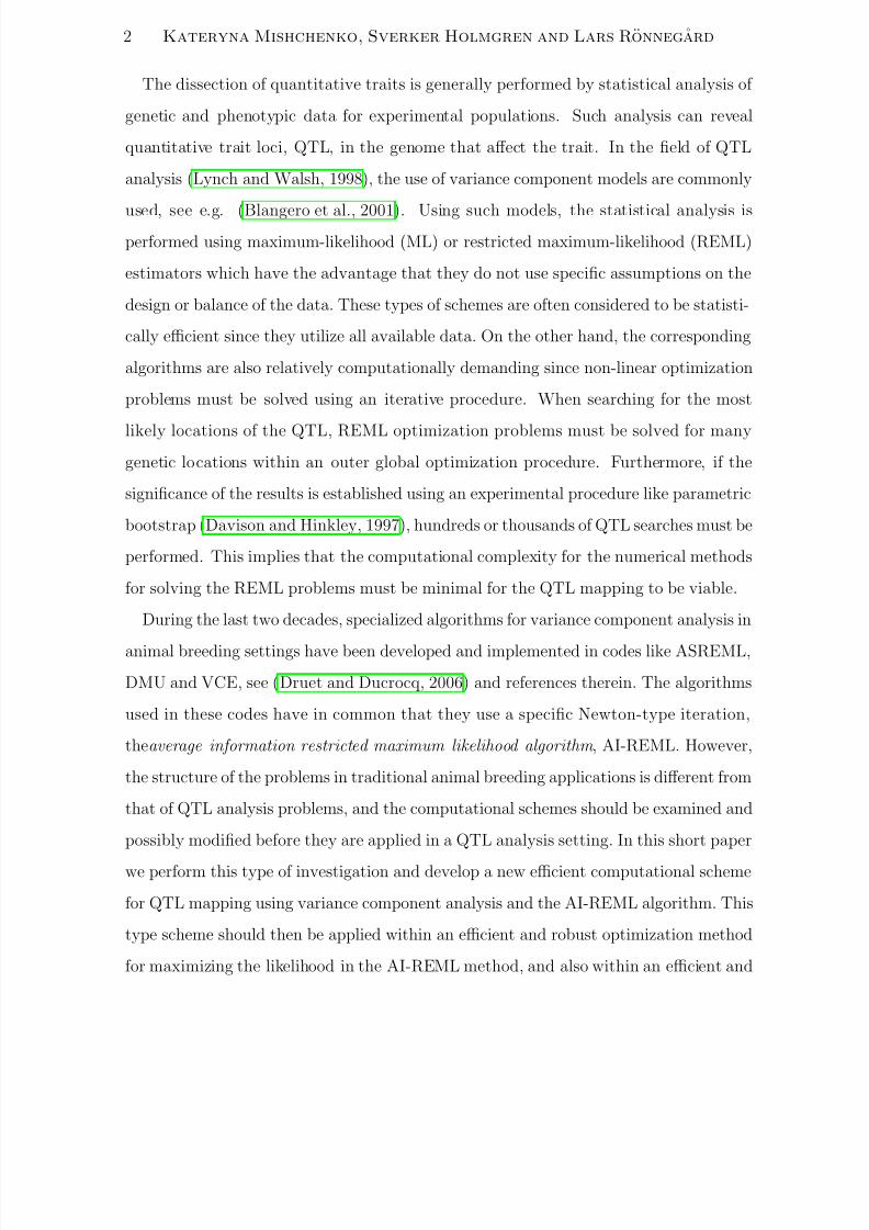
The dissection of quantitative traits is generally performed by statistical analysis of 

genetic and phenotypic data for experimental populations. Such analysis can reveal

quantitative trait loci, QTL, in the genome that affect the trait. In the field of QTL

analysis (Lynch and Walsh, 1998), the use of variance component models are commonly

used, see e.g. (Blangero et al., 2001). Using such models, the statistical analysis isperformed using maximum-likelihood (ML) or restricted maximum-likelihood (REML)

estimators which have the advantage that they do not use specific assumptions on the

design or balance of the data. These types of schemes are often considered to be statisti-

cally efficient since they utilize all available data. On the other hand, the corresponding

algorithms are also relatively computationally demanding since non-linear optimization

problems must be solved using an iterative procedure. When searching for the most

likely locations of the QTL, REML optimization problems must be solved for many

genetic locations within an outer global optimization procedure. Furthermore, if the

significance of the results is established using an experimental procedure like parametric

bootstrap (Davison and Hinkley, 1997), hundreds or thousands of QTL searches must be

performed. This implies that the computational complexity for the numerical methods

for solving the REML problems must be minimal for the QTL mapping to be viable.

During the last two decades, specialized algorithms for variance component analysis in

animal breeding settings have been developed and implemented in codes like ASREML,

DMU and VCE, see (Druet and Ducrocq, 2006) and references therein. The algorithms

used in these codes have in common that they use a specific Newton-type iteration,

theaverage information restricted maximum likelihood algorithm , AI-REML. However,

the structure of the problems in traditional animal breeding applications is different from

that of QTL analysis problems, and the computational schemes should be examined and

possibly modified before they are applied in a QTL analysis setting. In this short paper

we perform this type of investigation and develop a new efficient computational scheme

for QTL mapping using variance component analysis and the AI-REML algorithm. This

type scheme should then be applied within an efficient and robust optimization method

for maximizing the likelihood in the AI-REML method, and also within an efficient and

7/29/2019 0709.0625v2

http://slidepdf.com/reader/full/07090625v2 3/16

Efficient Implementation of the AI-REML Iteration 3

robust global optimization algorithm for the search for the outer optimization problem

where the most likely position of the QTL is determined.

2. The AI-REML algorithm

A general linear mixed model is given by

(1) y = Xb + Rr + e,

where y is a vector of n observations, X  is the n × nf  design matrix for nf  fixed effects,

R is the n × nr design matrix for nr random effects, b is the vector of  nf  unknown

fixed effects, r is the vector of  nr unknown random effects, and e is a vector of  n

residuals. In the QTL analysis setting, we assume that the entries of  e are identically

and independently distributed and there is a single observation for each individual in

the pedigree. In this case, the covariance matrices are given by var(e) = Iσ2

e and

var(r) = Aσ2

a, where A is referred to as the identity-by-descent  (IBD) matrix. Using

these assumptions, we have that

(2) var(y) ≡ V  = σ2

aA + σ2

eI  ≡ σ1A + σ2I.

Here, σ1 ≥ 0 and σ2 > 0 and we assume that the phenotype follows a normal distribution

with y MV N (Xb,V ). At least two different procedures can be used for computing

estimates of  b and σ1,2. In the standard codes mentioned above, the parameters are

computed from the mixed-model equations (MME) (Lynch and Walsh, 1998) using a

the inverse of  A. To be able to use this approach, A has to be positive definite, or it

must be modified so that this property holds. Also, the computations can be performed

efficiently if  A is sparse. For the QTL analysis problems, the IBD matrix A is often

only semi-definite and not necessarily sparse. Here the values of  σ1,2 are given by the

solution of the minimization problem

M i n L ,(3)

s.t. σ1 ≥ 0

σ2 > 0(4)

7/29/2019 0709.0625v2

http://slidepdf.com/reader/full/07090625v2 4/16

4 Kateryna Mishchenko, Sverker Holmgren and Lars Ronnegard

where L is the log-likelihood for the model (1),

(5) L = −2ln(l) = C + ln(det(V )) + ln(det(X T V −1X )) + yP T y,

and the projection matrix P  is defined by

(6) P  = V −1 − V −1X (X T V −1X )−1X T V −1.

In the original AI-REML algorithm, the minimization problem is solved using the stan-

dard Newton scheme but where the Hessian is substituted by the average information 

matrix  H AI , whose entries are given by

(7) H AI i,j = yT P ∂V 

∂σi

P ∂V 

∂σ jP y , i, j = 1, 2.

The entries of the gradient of  L are given by

(8)∂L

∂σi

= tr

∂V 

∂σi

P 

− yT P 

∂V 

∂σi

P y , i = 1, 2.

3. Efficient implementation of AI-REML optimization

The main result of this paper is an algorithm that allows for an efficient implementa-

tion of the iteration body in the AI-REML algorithm for variance component analysis

in QTL mapping problems. In (Mishchenko et al.), we examine optimization schemes

for the REML optimization and different approaches for introducing the constraints

for σ1,2 in the AI-REML scheme. For cases when the solution to the optimization

problem is close to a constraint, different ad-hoc fixes have earlier been attempted to

ensure convergence for the Newton scheme. In (Mishchenko et al.), we show that by

introducing an active-set formulation in the AI-REML optimization scheme, robustness

and good convergence properties were achieved also for cases when the solution is close

to a constraint. When computing the results below, we use the active-set AI-REML

optimization scheme from (Mishchenko et al.).

From the formulas in the previous section, it is clear that the most computationally

demanding part of the AI-REML algorithm is the computation of the matrix P , and

especially the explicit inversion of the matrix V  = σ1A + σ2I , where A is a constant

7/29/2019 0709.0625v2

http://slidepdf.com/reader/full/07090625v2 5/16

Efficient Implementation of the AI-REML Iteration 5

semi-definite matrix and σ1,2 are updated in each iteration. If V  is regarded as a general

matrix, i.e. no information about the structure of the problem is used, a standard

algorithm based on Cholesky factorization with complete pivoting is the only alternative,

and O(n3) arithmetic operations are required. If  A is very sparse, the work can be

significantly reduced by using a sparse Cholesky factorization, possibly combined witha reordering of the equations. This can be compared to the approach taken e.g. in

(Bates, (2004)), where a sparse factorization is used for A when solving the mixed-

model equations. However, as remarked earlier A is only semi-definite and not very

sparse for the QTL analysis problems and this approach is not an option here.

The IBD matrix A is a function of the location in the genome where the REML model

is applied. The key observation leading to a more efficient algorithm for inverting V  is

that the rank of A at a location with complete genetic information only depends on the

size of the base generation. At such locations, A will be a rank-k matrix where k ≪ n

in experimental pedigrees with small base generations. If the genetic information is not

fully complete, A can still be approximated by a low-rank matrix. The error in such an

approximation can be made small when the genetic distance to a location with complete

data is small.

Let a symmetric rank-k representation of  A be given by

(9) A = ZZ T ,

where Z  is an n × k matrix. We now exploit this type of representation to compute

V −1.

Case 1: An exact low-rank representation of  A is available a-priori. In

general, the inverse of a matrix plus a low-rank update can be computed using the

Woodbury formula, see e.g. (Golub and C.Van Loan, (1996)),

(10) B−1 = (C + S 1S T 2

)−1 = C −1 − C −1S 1(I  + S T 2

C −1S 1)−1S T 2

· C −1

7/29/2019 0709.0625v2

http://slidepdf.com/reader/full/07090625v2 6/16

6 Kateryna Mishchenko, Sverker Holmgren and Lars Ronnegard

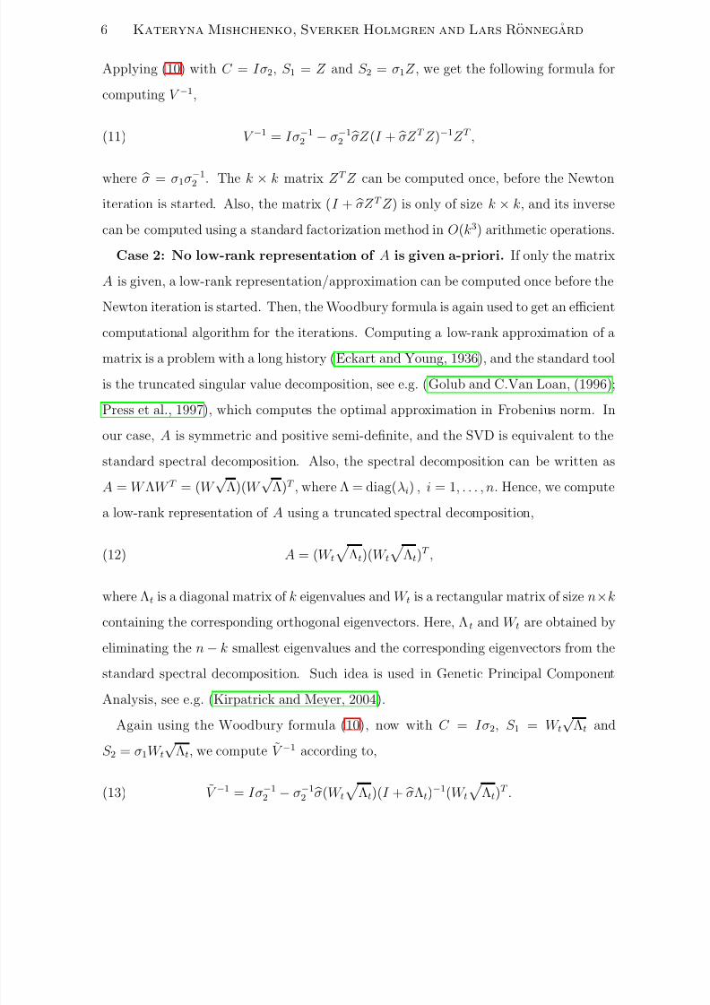
Applying (10) with C  = Iσ2, S 1 = Z  and S 2 = σ1Z , we get the following formula for

computing V −1,

(11) V −1 = Iσ−12

− σ−12σZ (I  + σZ T Z )−1Z T ,

where σ = σ1σ−12 . The k × k matrix Z T Z  can be computed once, before the Newton

iteration is started. Also, the matrix (I  + σZ T Z ) is only of size k × k, and its inverse

can be computed using a standard factorization method in O(k3) arithmetic operations.

Case 2: No low-rank representation of  A is given a-priori. If only the matrix

A is given, a low-rank representation/approximation can be computed once before the

Newton iteration is started. Then, the Woodbury formula is again used to get an efficient

computational algorithm for the iterations. Computing a low-rank approximation of a

matrix is a problem with a long history (Eckart and Young, 1936), and the standard tool

is the truncated singular value decomposition, see e.g. (Golub and C.Van Loan, (1996);

Press et al., 1997), which computes the optimal approximation in Frobenius norm. In

our case, A is symmetric and positive semi-definite, and the SVD is equivalent to the

standard spectral decomposition. Also, the spectral decomposition can be written as

A = W ΛW T  = (W √ 

Λ)(W √ 

Λ)T , where Λ = diag(λi) , i = 1, . . . , n. Hence, we compute

a low-rank representation of  A using a truncated spectral decomposition,

(12) A = (W t 

Λt)(W t 

Λt)T ,

where Λt is a diagonal matrix of k eigenvalues and W t is a rectangular matrix of size n×k

containing the corresponding orthogonal eigenvectors. Here, Λt and W t are obtained by

eliminating the n − k smallest eigenvalues and the corresponding eigenvectors from the

standard spectral decomposition. Such idea is used in Genetic Principal Component

Analysis, see e.g. (Kirpatrick and Meyer, 2004).Again using the Woodbury formula (10), now with C  = Iσ2, S 1 = W t

√ Λt and

S 2 = σ1W t√ 

Λt, we compute V −1 according to,

(13) V −1 = Iσ−12

− σ−12σ(W t

 Λt)(I  + σΛt)

−1(W t 

Λt)T .

7/29/2019 0709.0625v2

http://slidepdf.com/reader/full/07090625v2 7/16

Efficient Implementation of the AI-REML Iteration 7

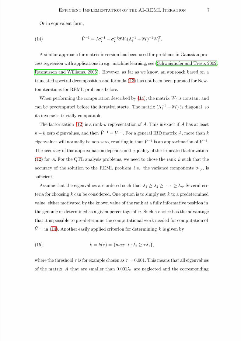
Or in equivalent form,

(14) V −1 = Iσ−12

− σ−12σW t(Λ−1t + σI )−1W T t .

A similar approach for matrix inversion has been used for problems in Gaussian pro-

cess regression with applications in e.g. machine learning, see (Schwaighofer and Tresp, 2002;

Rasmussen and Williams, 2005). However, as far as we know, an approach based on a

truncated spectral decomposition and formula (13) has not been been pursued for New-

ton iterations for REML-problems before.

When performing the computation described by (14), the matrix W t is constant and

can be precomputed before the iteration starts. The matrix (Λ−1t + σI ) is diagonal, so

its inverse is trivially computable.

The factorization (12) is a rank-k representation of  A. This is exact if  A has at least

n − k zero eigenvalues, and then V −1 = V −1. For a general IBD matrix A, more than k

eigenvalues will normally be non-zero, resulting in that V −1 is an approximation of V −1.

The accuracy of this approximation depends on the quality of the truncated factorization

(12) for A. For the QTL analysis problems, we need to chose the rank k such that the

accuracy of the solution to the REML problem, i.e. the variance components σ1,2, is

sufficient.Assume that the eigenvalues are ordered such that λ1 ≥ λ2 ≥ · · · ≥ λn. Several cri-

teria for choosing k can be considered. One option is to simply set k to a predetermined

value, either motivated by the known value of the rank at a fully informative position in

the genome or determined as a given percentage of  n. Such a choice has the advantage

that it is possible to pre-determine the computational work needed for computation of 

V −1 in (14). Another easily applied criterion for determining k is given by

(15) k = k(τ ) = {max i : λi ≥ τ λ1},

where the threshold τ  is for example chosen as τ  = 0.001. This means that all eigenvalues

of the matrix A that are smaller than 0.001λ1 are neglected and the corresponding

7/29/2019 0709.0625v2

http://slidepdf.com/reader/full/07090625v2 8/16

8 Kateryna Mishchenko, Sverker Holmgren and Lars Ronnegard

columns of  W  in the spectral decomposition are deleted. In the numerical experiments

presented in the next section, we use the truncation criterion (15).

For computing the truncated spectral decomposition, we currently use a standard

eigenvalue solver, compute all eigenvalues and eigenvectors, and then ignore the data

connected to eigenvalues smaller than given by the truncation criterion. For problemswith large data matrices where it is known that only a small number of eigenvalues

will be large, an alternative can be to use e.g. the Lanczos iteration for computing

these. Potentially, this can reduce the arithmetic work for computing the truncated

decomposition before the iteration starts.

Once V −1 has been computed using either (14) or (11), formula (6) is used to compute

P , and the entries of the Hessian H AI  and the gradient of  L are computed using the

formulas (7) and (8). The matrices involved have common terms which are computed

once at the beginning of the current iteration to reduce the total complexity.

4. Numerical Results

In this section we present numerical experiment computed using experimental IBD

matrices of size 767 × 767 drawn from a chicken population (Kerje et al., 2003). For

these first pilot investigations of the computational performance we have chosen to

implement the algorithms in Matlab, and we present execution time measurements for

the Matlab scripts. At a later stage, we will implement the most promising algorithms

also in C, which will reduce the execution time further. In this case, we expect that

the relative gain from using the new algorithms will be larger than indicated below.

Matlab’s native implementation of standard inversion is presumably more efficient than

our Matlab scripts for the new algorithms, which are interpreted at runtime.

Case 1: We first present numerical results for the case when the IBD matrices A have

exact low-rank representations given a-priori. Let T C  be the measured computational

time for the computation of V −1 within the AI-REML scheme using standard inversion,

and let T W  be the corresponding time when using the low-rank representation and

7/29/2019 0709.0625v2

http://slidepdf.com/reader/full/07090625v2 9/16

Efficient Implementation of the AI-REML Iteration 9

formula (11). In Figure 1 we show T C /T W , i.e. the speedup for the computations of 

V −1, as a function of the rank k of the matrices A.

0 100 200 300 400 500 600 7000

5

10

15

20

25

Rank k of the low−rank representation of A

   T   C

   /   T   W

The speedup achieved for computing V−1

by using the low−rank representation of A

Figure 1. The speedup achieved for the computations of  V −1 in the

AI-REML scheme achieved by using the scheme based on (11) instead of 

standard inversion

From Figure 1, it is clear that for IBD matrices of size 767 × 767, the implementation

using the low-rank representation is faster if the rank k is smaller than approximately

350. Also, for k < 50, the speedup is more than one order of magnitude.

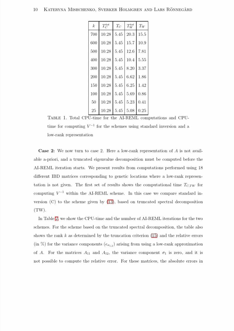
In Table 1 we present the total CPU-times for the AI-REML scheme and the CPU-

time for the computations of V −1 within this scheme for different values of k and number

of iterations equal to 9. The total CPU-times for the AI-REML are denoted by T totC  and

T totW  , while the CPU-times for the computation of  V −1 are denoted by T C  and T W .

From Table 1 it is clear that for the problems studied here, computing V −1 using

standard inversion accounts for approximately half of the computational time in the

AI-REML scheme. For small values of  k, the time needed for inverting V −1 using the

low-rank representation can effectively be ignored, and the improved algorithm runs

approximately twice as fast as the original scheme using standard inversion.

7/29/2019 0709.0625v2

http://slidepdf.com/reader/full/07090625v2 10/16

7/29/2019 0709.0625v2

http://slidepdf.com/reader/full/07090625v2 11/16

7/29/2019 0709.0625v2

http://slidepdf.com/reader/full/07090625v2 12/16

12 Kateryna Mishchenko, Sverker Holmgren and Lars Ronnegard

scheme and different errors in the location of the optima. However, for the problems

studied here, choosing τ  = 0.001 results in that the variance components are determined

with sufficient accuracy for all the IBD matrices examined.

In the next set of experiments we study the speedup and error introduced by using

an approximate inverse of  V  in some more detail for the two IBD matrices A1 and A13.As can be seen from Table 2, A1 is harder to approximate with a low rank matrix than

A13. In Tables 3 and 4, we vary the value of the parameter τ  in the truncation criterion

(15) and show the resulting rank k of the approximation of  A, the number of iterations

in the AI-REML optimization scheme, the speedup T C /T TW , and the relative errors in

the variance components.

τ k # it T C /T TW  eσ1 [%] eσ2 [%]10−7 699 7 0.46 0.000 0.000

10−6 662 7 0.51 0.002 0.001

10−5 556 7 0.71 0.070 0.054

10−4 294 7 1.97 0.82 1.67

5 · 10−4 82 7 7.68 6.75 4.69

10−3 29 36 3.28 95.2 6.70

5 · 10−3

- no conv. - - -Table 3. Results for the IBD matrix A1 for different values of the trun-

cation parameter τ 

In Figure 2 we finally present total timings for solving the AI-REML problems using

the new scheme exploiting a truncated spectral decomposition, including the time needed

for computing the truncated factorization prior to the AI-REML iterations. We also

compare these timings to the corresponding results for the standard scheme using direct

inversion. In the figure, the timings for all matrices A1 − A18 are shown as a function of 

the number of AI-REML iterations required. When several matrices result in the same

number of iterations, the cpu time for each matrix and the average result are shown.

7/29/2019 0709.0625v2

http://slidepdf.com/reader/full/07090625v2 13/16

7/29/2019 0709.0625v2

http://slidepdf.com/reader/full/07090625v2 14/16

14 Kateryna Mishchenko, Sverker Holmgren and Lars Ronnegard

Theoretically, the average cpu time for the scheme exploiting the truncated spectral

decomposition should be a straight line. Deviations are due to the inconsistence of time

measurement in Matlab.

From Figure 2, we see that the standard scheme using direct inversion is faster when

number of iterations is small, i.e. less than 9 iterations. The reason for this is that thespectral decomposition of the matrix A is relatively costly, and it must be amortized over

a number of iterations before the faster iterations begin to pay of. When the number of 

iterations required is significantly larger than 9, which is often the case for real-world

problems, the new algorithm is significantly faster also when no low-rank representations

of the IBD matrices are not available a priori.

5. Conclusions

In this paper we present a family of algorithms that allow for an efficient imple-

mentation of the iteration body in the AI-REML algorithm for variance component

analysis in QTL mapping problems. Combined with the improved optimization scheme

in (Mishchenko et al.), the new algorithms form a basis for an efficient and robust AI-

REML scheme for evaluating variance component QTL models.

The most costly operation in the AI-REML iteration body is the explicit inversion

of the matrix V  = σ1A + σ2I , where the IBD matrix A is constant and positive semi-

definite, and σ1 ≥ 0 and σ2 > 0 are updated in each iteration. The key information

enabling the introduction of improved algorithms is that the rank of  A at a location

in the genome with complete genetic information only depends on the size of the base

generation. At such locations, A will be a rank-k matrix where k ≪ n, and by exploiting

the Woodbury formula the inverse of V  can be computed more efficiently than by using

a standard algorithm based on Cholesky factorization. If the genetic information is

not fully complete, a general IBD matrix A can still be approximated by a low-rank

matrix and the error in such an approximation can be made small when the genetic

distance to a location with complete data is small. More importantly, there might be

a possibility for setting up a low-rank representation of the matrix A also at genetic

7/29/2019 0709.0625v2

http://slidepdf.com/reader/full/07090625v2 15/16

Efficient Implementation of the AI-REML Iteration 15

locations where the information is not complete. This is a topic of current investigation

(Ronnegard and Carlborg, 2007).

We present results for IBD matrices A from a real data set for two different settings;

Firstly, we show that if a low-rank representation of A is available a-priori, the inversion

of  V  using the new algorithms is performed faster than using a standard algorithm if the rank k is smaller than approximately 350. Also, for k < 50, the speedup is more

than one order of magnitude.

Then we also show that, even if a low-rank representation is not directly available and

a low-rank approximation of  A needs to be computed before the AI-REML iterations,

significant speedup of the variance component model computations can still be achieved.

For QTL mapping problems, the efficiency of our new method will increase when the

ratio between the total pedigree size and base generation size increases, the density and

informativeness of markers increases. Hence, the relative efficacy of the method will

continuously increase in the future with deeper pedigrees and more markers. Also, we

are currently developing a scheme for directly constructing a low-rank representation

of the IBD matrix A also between markers, which will result in that the eigenvalue

factorization prior to the AI-REML iterations is not needed any more.

References

Bates, D. (2004). Sparse matrix representations of linear mixed models . Technical Report.

http://www.stat.wisc.edu/ bates/reports/MixedEects.pdf.

Blangero, J., J.T. Williams, and L. Almasy. 2001. Variance component methods for detecting complex 

trait loci , Advances in Genetics 42, 151–181.

Davison, A. C. and D. V. Hinkley. 1997. Bootstrap methods and their application., Cambridge Univer-

sity Press, U.K.

Druet, T. and V. Ducrocq. 2006. Innovations in software packages in quantitative genetics . World

Congress on Genetics Applied to Livestock Production,Belo Horizonte, Brazil.

Eckart, C. and G. Young. 1936. The approximation of one matrix by another of lower rank , Psycho-

metrica 1, no. 3, 211–218.

Golub, G. and C.Van Loan. (1996). Matrix Computations , Third edition, The Johns Hopkins University

Press.

7/29/2019 0709.0625v2

http://slidepdf.com/reader/full/07090625v2 16/16

16 Kateryna Mishchenko, Sverker Holmgren and Lars Ronnegard

Kerje, S., O. Carlborg, L. Jacobsson, K. Schutz, C. Hartmann, P. Jensen, and L. Andersson. 2003.

The twofold difference in adult size between the red junglefowl and white leghorn chickens is largely 

explained by a limited number of qtls , Animal Genetics 34, 264–274.

Kirpatrick, M. and K. Meyer. 2004. Direct estimation of genetic principal components: Simplified 

analysis of complex phenotypes , Genetics 168, 2295–3206.

Lynch, M. and B. Walsh. 1998. Genetics and analysis of quantitative traits , Sinauer Associates, Inc.

Mishchenko, K., S. Holmgren, and L. Ronnegard. Newton-type methods for reml estimation in genetic 

analysis of quantitative traits . http://arxiv.org/abs/0711.2619.

Press, W. H., S. A. Teukolsky, W. T. Vetterling, and B. P. Flannery. 1997. Numerical recipes in c.

the art of scientific computing , Second edition, Cambridge University Press.

Rasmussen, C.E. and C. Williams. 2005. Gaussian processes for machine learning , MIT Press.

Ronnegard, L. and O. Carlborg. 2007. Separation of base allele and sampling term effects gives new 

insights in variance component qtl analysis , BMC Genetics 8, no. 1.

Schwaighofer, A. and V. Tresp. 2002. Transductive and inductive methods for approximate gaussian 

process regression , NIPS.

Department of Mathematics and Physics, Malardalen University, Box 883, SE-721 23

Vasteras, Sweden

E-mail address : kateryna.mishchenko@mdh.se

Division of Scientific Computing, Department of Information Technology, Uppsala

University, SwedenE-mail address : sverker@it.uu.se

Linnæus Center for Bioinformatics, Uppsala University, Sweden

E-mail address : lars.ronnegard@lcb.uu.se