0042 Set 1

8/3/2019 0042 Set 1

http://slidepdf.com/reader/full/0042-set-1 1/27

Q.1 Price elasticity of demand depends on various factors. Explain each factor with the help

of an example.

Elasticity of Demand

Earlier we have discussed the law of demand and its determinants. It tells us only the directionof change in price and quantity demanded. But it does not specify how much more is purchased

when price falls or how much less is bought when price rises. In order to understand the

quantitative changes or rate of changes in price and demand, we have to study the concept of

elasticity of demand.

Meaning and Definition

The term elasticity is borrowed from physics. It shows the reaction of one variable with respect

to a change in other variables on which it is dependent. Elasticity is an index of reaction.

In economics the term elasticity refers to a ratio of the relative changes in two quantities. It

measures the responsiveness of one variable to the changes in another variable.

Elasticity of demand is generally defined as the responsiveness or sensitiveness of demand to a

given change in the price of a commodity. It refers to the capacity of demand either to stretch

or shrink to a given change in price. Elasticity of demand indicates a ratio of relative changes in

two quantitiesie, price and demand. According to prof. Boulding. Elasticity of demand

measures the responsiveness of demand to changes in price 1 In the words of Marshall, The

elasticity (or responsiveness) of demand in a market is great or small according to the amount

demanded much or little for a given fall in price, and diminishes much or little for a given rise in

price 2.

Kinds of elasticity of demand

Broadly speaking there are five kinds of elasticity of demand.

They are Price Elasticity, Income Elasticity, Cross Elasticity, Promotional

Elasticity and Substitution Elasticity. We shall discuss each one of them in

some detail.

Price Elasticity of Demand

In the words of Prof. Stonier and Hague, price elasticity of demand is a technical term used by

economists to explain the degree of responsiveness of the demand for a product to a change in

its price.

8/3/2019 0042 Set 1


Percentage change in quantity demanded .

Ep = where Ep is price elasticity

Percentage change in price

Demand rises by 80%, i.e. +804 Demand falls by 80%, i.e. 804

Prices falls by 20%, i.e. 20 price rises by 20%,i.e. +20

It implies that at the present level with every change in price, there will be a change in demand

four times inversely. Generally the co-efficient of price elasticity of demand always holds a

Original demand = 20 units original price = Rs. 6

New demand = 60 units New price = 4

Change in demand = 60 - 20 = 40 Change in price 4 - 6 = - 2 40 6 32X20="6.

The rate of change in demand may not always be proportionate to the change in price. A small

change in price may lead to very great change in demand or a big change in price may not lead

to a great change in demand. Based on numerical values of the co-efficient of elasticity, we can

have the following five degrees of price elasticity of demand. Different Degree of Price Elasticity

of Demand 1. Perfectly Elastic Demand

In this case, a very small change in price leads to an infinite change in demand. The demand

curve is a horizontal line and parallel to OX axis. The numerical co-efficient of perfectly elastic

demand is infinity (ED=oo)

8/3/2019 0042 Set 1


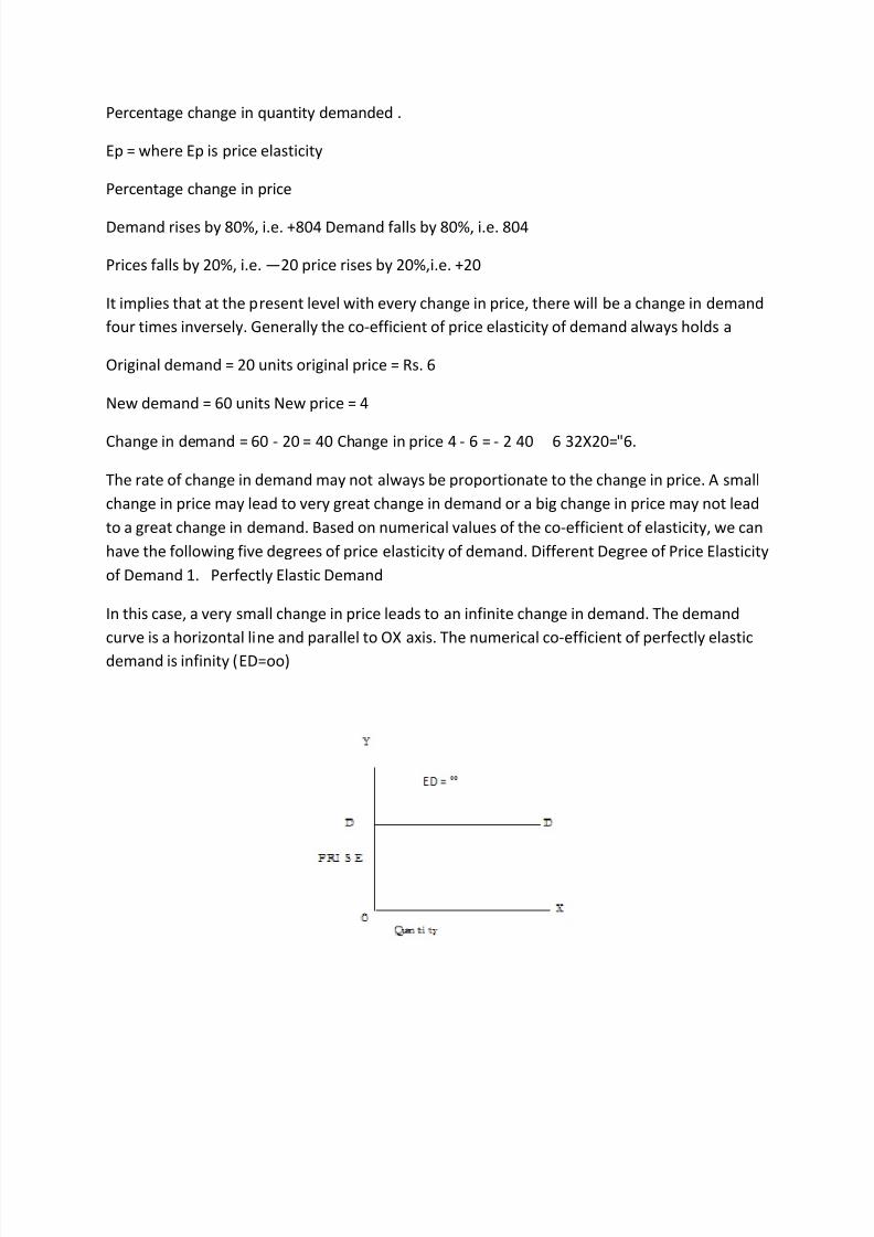
2. Perfectly Inelastic Demand: In this case, what ever may be the change in price, quantity

demanded will remain perfectly constant. The demand curve is a vertical straight line and

parallel to OY axis. Quantity demanded would be 10 units, irrespective of price changes from

Rs. 10.00 to Rs. 2.00. Hence, the numerical co-efficient of perfectly inelastic demand is zero. ED

= 0

3. Relative Elastic Demand: In this case, a slight change in price leads to more than

proportionate change in demand. One can notice here that a change in demand is more than

that of change in price. Hence, the elasticity is greater than one. For e.g.. price alls by 3 % and

demand rises by 9 %. Hence, the numerical co-efficient of demand is greater

than one.

8/3/2019 0042 Set 1


4. Relatively Inelastic Demand: In this case, a large change in price, say

8 % fall price, leads to less than proportionate change in demand, say

4 % rise in demand. One can notice here that change in demand is less

than that of change in price. This can be represented by a steeper

demand curve. Hence, elasticity is less than one.

In all economic discussion, relatively elastic demand is generally called as elastic demand or

more elastic demand while relatively inelastic demand is popularly known as inelastic

demand or less elastic demand.

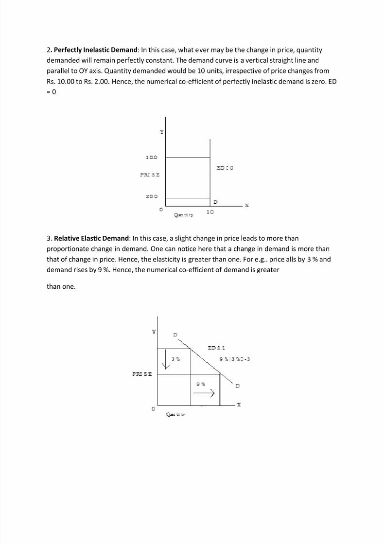
5. Unitary elastic demand: In this case, proportionate change in price leads to equal

proportionate change in demand. For e.g., 5 % fall in price leads to exactly 5 % increase in

demand. Hence, elasticity is equal to unity. It is possible to come across unitary elastic demand

but . s a rare phenomenon.

8/3/2019 0042 Set 1


Out of five different degrees, the first two are theoretical and the last one is a rare possibility.Hence, in all our general discussion, we make reference only to two terms-relatively elastic

demand and relatively inelastic demand.

Determinants of Price Elasticity of Demand

The elasticity of demand depends on several factors of which the following are some of the

important ones.

1. Nature of the Commodity

Commodities coming under the category of necessaries and essentials tend to be inelastic

because people buy them whatever may be the price. For example, rice, wheat, sugar, milk,

vegetables etc. on the other hand, for comforts and luxuries, demand tends to be elastic e.g.,

TV sets, refrigerators etc.

2. Existence of Substitutes

Substitute goods are those that are considered to be economically interchangeable by buyers. If

a commodity has no substitutes in the market, demand tends to be inelastic because people

have to pay higher price for such articles. For example. Salt, onions, garlic, ginger etc. In case of

commodities having different substitutes, demand tends to be elastic. For example, blades,

tooth pastes, soaps etc.

8/3/2019 0042 Set 1


3. Number of uses for the commodity

Single-use goods are those items which can be used for only one purpose and multiple-use

goods can be used for a variety of purposes. If a commodity has only one use (singe use

product) then demand tends to be inelastic because people have to pay more prices if they

have to use that product for only one use. For example, all kinds of eatables, seeds, fertilizers,

pesticides etc. On the contrary, commodities having several uses,

ED =1

5%15%=1

[multiple-use-products] demand tends to be elastic. For example, coal, electricity, steel etc.

4. Durability and reparability of a commodity

Durable goods are those which can be used for a long period of time. Demand tends to be

elastic in case of durable and repairable goods because people do not buy them frequently. For

example, table, chair, vessels etc. On the other hand, for perishable and non-repairable goods,

demand tends to be inelastic e.g., milk, vegetables, electronic watches etc.

5. Possibility of postponing the use of a commodity

In case there is no possibility to postpone the use of a commodity to future, the demand tends

to be inelastic because people have to buy them irrespective of their prices. For example,

medicines. If there is possibility to postpone the use of a commodity, demand tends to be

elastic e.g., buying a TV set, motor cycle, washing machine or a car etc.

6. Level of Income of the people

Generally speaking, demand will be relatively inelastic in case of rich people because any

change in market price will not alter and affect their purchase plans. On the contrary, demand

tends to be elastic in case of poor.

7. Range of Prices

There are certain goods or products like imported cars, computers, refrigerators, TV etc, which

are costly in nature. Similarly, a few other goods like nails; needles etc. are low priced goods. In

all these cases, a small fall or rise in prices will have insignificant effect on their demand. Hence,

demand for them is inelastic in nature. However, commodities having normal prices are elastic

in nature.

8/3/2019 0042 Set 1


8. Proportion of the expenditure on a commodity

When the amount of money spent on buying a product is either too small or too big, in that

case demand tends to be inelastic. For example, salt, newspaper or a site or house. On the

other hand, the amount of money spent is moderate; demand in that case tends to be elastic.

For example, iegetables and fruits, cloths, provision items etc.

9. Habits

When people are habituated for the use of a commodity, they do not care for price changes

over a certain range. For example, in case of smoking, drinking, use of tobacco etc. In that case,

demand tends to be inelastic. If

people are not habituated for the use of any products, then demand

generally tends to be elastic.

10. Period of time

Price elasticity of demand varies with the ienqh of the time period,

Generally speaking, in the short period, demand is inelastic because

consumption habits of the people, customs and traditions etc. do not

change. On the contrary, demand tends to be elastic in the long period

where there is possibility of all kinds of changes.

II. Level of Knowledge Demand in case of enlightened customer would be elastic and in case of

ignorant customers, it would be inelastic.

12. Existence of complementary goods Goods or services whose demands are interrelated so

that an increase in the price of one of the products results in a fall in the demand for the other.

Goods which are jointly demanded are inelastic in nature. For example, pen and ink, vehicles

and petrol, shoes and socks etc have inelastic demand for this reason. If a product does not

have complements, in that case demand tends to be elastic. For example, biscuits, chocolates,ice creams etc. In this case the use of a product is not linked to any other products.

13. Purchase frequency of a product If the frequency of purchase is very high, the demand

tends to be inelastic. For e.g., coffee, tea, milk, match box etc. on the other hand, if people buy

a product occasionally, demand tends to be elastic. For example, durable goods like radio, tape

recorders, refrigerators etc.

8/3/2019 0042 Set 1


Q.2 A company is selling a particular brand of tea and wishes to introduce a new

flavor. How will the company forecast demand for it ?

Demand forecasting for new products is quite different from mat For established products.

Here the firms will not have any past experience or past data for this purpose. An intensivestudy of the economic and

competitive characteristics of the product should be made to make efficient

forecasts.

Professor Joel Dean. however, has suggested a few guidelines to make

forecasting of demand for new products.

a) Evolutionary approach

The demand for the new product may be considered as an outgrowth of an

existing product. For e.g., Demand for new Tata Indica, which is a modified

version of Old Indica can most effectively be projected based on the sales of

the old Indica, the demand for new Pulsar can be forecasted based on the a

sales of the old Pulsor. Thus when a new product is evolved from the old

product, the demand conditions of the old product can be taken as a basis

for forecasting the demand for the new product.

b) Substitute approach

If the new product developed serves as substitute for the existing product,

the demand for the new product may be worked out on the basis of a

market share. The growths of demand for all the products have to be

worked out on the basis of intelligent forecasts for independent variables

that influence the demand for the substitutes. After that, a portion of the

market can be sliced out for the new product. For e.g., A moped as a

substitute for a scooter, a cell phone as a substitute for a land line. In some

8/3/2019 0042 Set 1


price plays an important role in shaping future demand for the product.

c) Opinion Poll approach

Under this approach the potential buyers are directly contacted, or through

the use of samples of the new product and their responses are found out.

These are finally blown up to forecast the demand for the new product.

d) Sales experience approach

Offer the new product for sale in a sample market; say supermarkets or big

bazaars in big cities, which are also big marketing centers. The product may

be offered for sale through one super market and the estimate of sales

obtained may be blown up to arrive at estimated demand for the product.

e) Growth Curve approach

According to this, the rate of growth and the ultimate level of demand for type new

product are estimated on the basis of the pattern of growth of established products. For e.g.,

An Automobile Co., while introducing a new version of a car will study the level of demand for

the existing car.

f) Vicarious approach

A firm will survey consumers reactions to a new product indirectly through getting in touch

with some specialized and informed dealers who have good knowledge about the market,

about the different varieties of the product already available in the market, the consumers

preferences etc. This helps in making a more efficient estimation of future demand.

These methods are not mutually exclusive. The management can use a combination of several

of them, supplement and cross check each other.

8/3/2019 0042 Set 1


Q.3 The supply of a product depends on the price. What are the other factors that will

affect the supply of a product.

Supply is one of the two forces that determine the price of a commodity in the market. Supply

means the amount offered for sale at a given price. According to Thomas, The supply of goodsis the quantity offered for sale in a given market at a given time at various prices. According to

Prof. Macconnel supply may be defined as a schedule which shows the various amounts of

a product which a producer is willing to and able to produce and make available for sale in the

market at each specific price in a set of possible prices during some given period.Thus supply

of a product refers to the various amounts which are offered for sale at a particular price during

a given period of time.

Supply can be equal, more or less, than the current production depending upon the nature of

the commodity, price and the requirements of the producers.

Supply is also different from stock. Stock is the total volume of a commodity which can be

brought into the market for sale at a short notice and supply means the quantity which is

actually brought in the market. For perishable commodities, like fish and fruits, supply and

stock are the same because they cannot be stored. The commodities which are not perishable

can be held back, if prices are not favorable and released in large quantities when prices are

favorable. In short, stock is potential supply.

Supply Function

The law of supply and supply schedule explains only the direct relationship between price andsupply. Mathematically S = f (P). Both analyses the impact of change in price on quantity

supplied. Supply of a product, apart from price changes also depends upon many factors. When

we analyze the influence of these factors on supply, supply schedule will be converted into a

supply function.

Supply function is a comprehensive one as it analyses the causes for chaiges in supply in a

detailed manner. Mathematically a supply function caq be represented in the following

manner.

Sx = f(Pf,T,Cp,Gp,N etc)

Where

j Sx = supply of a given product x

Pf = price of factor input

8/3/2019 0042 Set 1


T Technology

Cp = cost of production

Gp = Government policy

N Number of firms etc

Determinants of Supply

Apart from price, many factors bring about changes in supply. Among them the important

factors are:

1. Natural factors: Favorable natural factors like good climatic conditions, timely, adequate,

well distributed rainfall results in higher production and expansion in supply. On the other

hand, adverse factors like bad weather conditions, earthquakes, droughts, untimely, ill-

distributed, inadequate rainfall, pests etc., may cause decline in production and contraction in

supply.

2. Change in techniques of production: An improvement in techniques of production and use

of modern, highly sophisticated machines and equipments will go a long way in raising the

output and expansion in supply. On the contrary, primitive techniques are responsible for lower

output and hence lower supply.

3. Cost of prbduction: Given the market price of a product, if the cost of production rises due to

higher wages, interest and price of inputs, supply decreases. If the cost of production falls, on

account of lower wages, interest and price of inputs, supply rises.

4. Prices of related goods: If prices of related goods fall, the seller of a given commodity offer

more units in the market even though, the price of his product has not gone up. Opposite will

be the case when the price of related goods rises.

5. Government policy: When the government follows a positive policy, it encourages

production in the private sector. Consequently, supply expands. For example granting of

subsidies, development rebates, tax concession, etc,. On the other hand, output and supply

cripples when the government adopts a negative policy. For example withdrawal of all

concessions and incentives, imposition of high taxes, introduction of controls and quota system

etc.

6. Monopoly power: Supply tends to be low, when the market is controlled by monopolists, or

a few sellers as in the case of oligopoly. Generally supply would be more under competitive

conditions.

8/3/2019 0042 Set 1


7. Number of sellers or firms: Supply would be more when there are a large number of sellers.

Similarly production and supply tends to be

more when production is organized on large scale basis. If rate or speed of production is high,

supply expands. Opposite will be the case when number of sellers is less, small scale production

and low

rate of production.

8. Complementary goods: In case of joint demand, the production & sale of one product may

lead to production and sale of other product also.

9. Discovery of new source of inputs: Discovery of new sources of inputs helps the producers

to supply more at the same price & vice- versa.

10. Improvements in transport and communication: This will facilitate

free and quick movements of goods and services from production

centers to marketing centers.

11. Future rise in prices: When sellers anticipate a further rise in price, in that case current

supply tends to fall. Opposite will be the case when, the seller expect a fall in price.

Thus, many factors influence the supply of a product in the market. A firm should have a

thorough knowledge of all these factors because it helps in preparing its production plan and

sales strategy.

8/3/2019 0042 Set 1


Q.4 Show how producers equilibrium is achieved with isoquants and isocost

curves.

The law gives guidance that by making continuous improvements in science and technology,

the producer can postpone the occurrence of

diminishing returns.

Production function with Two Variable Inputs ISO-Quants and ISO-Costs

The prime concern of a firm is to workout the cheapest factor combinations to produce a given

quantity of output. There are a large number of alternative combinations of factor inputs which

can produce a given quantity of output for a given amount of investment. Hence, a producer

has to select the most economical combination out of them. Iso-product curve is a technique

developed in recent years to show the equilibrium of a producer with two variable factor

inputs. It is a parallel concept to the indifference curve in the theory of consumption.

Meaning and Definitions

The term Iso Quant has been derived from Iso meaning equal and Quant meaning

quantity. Hence, Iso Quant is also called Equal Product Curve or Product Indifference Curve

or Constant Product Curve. An Iso product curve represents all the possible combinations of

two factor inputs which are capable of producing the same level of output. It may be defined as

a curve which shows the different combinations of the two inputs producing the same level

of output .

Each Iso Quant curve represents only one particular level of output. If there are different

lsoQuant curves, they represent different levels of output. Any point on an Iso Quant curve

represents same level of output. Since each point indicates equal level of output, the producer

becomes indifferent with respect to any one of the combinations.

Equal Product Combination

In the above schedule, all the five factor combinations will produce the equal level of output,

i.e.100 units. Hence, the producer is indifferent with respect to any one of the combinations

mentioned above.

In the diagram, if we join points ABCDE (which represents different combinations of factor x

and y) we get an Iso-quant curve iQ. This curve represents 100 units of output that may be

produced by employing any one of the combinations of two factor inputs mentioned above. It

is to be noted that an Iso-Product Curve shows the exact physical units of output that can be

8/3/2019 0042 Set 1


8/3/2019 0042 Set 1


It shows two things (a) prices of two inputs (b) total outlay of the firm. Each Iso-cost line will

show various combinations of two factors which can be purchased with a given amount of

money at the given price of each input. We can draw the Iso-cost line on the basis of an

imaginary example.

Let us suppose that a producer wants to spend Rs. 3,000 to purchase factor

X and Y. If the price of X per unit Rs. 100 he can purchase 30 units of X.

Similarly if the price of factor Y is Rs. 50 then he can purchase 60 units of Y.

When 30 units of factor X are represented on OY axis and 60 units of factor Y are

represented on OX- axis, we get two points A & B. If we join these two points A and B, then we

get the Iso-Cost line AB. This line represents the different combinations of factor X and Y that

can be purchased with Rs. 3,000.

The Iso-Cost line will shift to the right if the producer increase his outlay from Rs. 3,000 to Rs.

4,000. On the contrary, if his outlay decreases to Rs. 2,000, there will be a backward shift in the

position of Iso-cost line.

The slope of the Iso-cost line represents the ratio of the price of a unit of actor X to the price of

a unit of factor Y. In case, the price of any one of them changes there would be a corresponding

change in the slope and Dosition of Iso-cost line

PRODUCERS EQUILIBRIUM (Optimum factor combination or least cost

combination).

The optimal combination of factor inputs may help in either minimizing cost for a given level of

output or maximizing output with a given amount of rivestment expenditure. In order to

explain producers equilibrium, we have to integrate Iso-quant curve with that of Iso-cost line.

Iso-product curve represent different alternative possible combinations of two factor inputs

with the help of which a given level of output can be produced. On the other ,and, Iso-cost line

shows the total outlay of the producer and the prices of Factors of production.

The intention of the producer is to maximize his profits. Profits can be maximized when he is

producing maximum output with minimum production cost. Hence, the producer selects the

least cost combination of the factor inputs. Maximum output with minimum cost is possible

only when he reaches the position of equilibrium. The position of equilibrium is indicated at the

point where Iso-Quant curve is tangential to Iso-Cost line. The following diagram explains how

the producer reaches the position of equilibrium.

8/3/2019 0042 Set 1


It is quite clear from the diagram that the producer will reach the position of equilibrium at the

point E where the Iso-quant curve IQ and Iso-cost line AB is tangent to each other. With a given

total out lay of Rs. 5,000 the producer will be producing the highest output, i.e. 500 units by

employing 25 units of factors X and 50 units of factor Y. (assuming Rs. 2,500 each is spent on X

and Y)

The price of one unit of factor X is Rs.l00 and that of Y is Rs. 50. Rs.100 x 25 units of 2500 and

Rs. 50 x 50 units of Y = 2500. He will not reach the position of equilibrium either at the point El

and E2 because they are on a higher Iso-cost line. Similarly, he cannot move to the left side of E,

because they are on a lower Iso-Cost line and he will not be able to produce 500 units of output

by any combinations which left to the IE of E.

Thus, the point at which the Iso-Quant is tangent to the Iso-Cost lii represents the minimum

cost or optimum factor combination for producing given level of output. At this point, MRTS

between the two points is equal the ratio between the prices of the inputs.

Long Run Production Function [Change In All Factor Inputs In The Same Proportion]

Laws of Returns to Scale

The concept of returns to scale is a long run phenomenon. In this case, we study the change in

output when all factor inputs are changed or made available in required quantity. An increase

in scale means that all factor inputs are increased in the same proportion. In returns to scale, all

the necessary factor inputs are increased or decreased to the same extent so that whatever the

scale of production, the proportion among the factors remains the same.

Three Phases of Returns to Scale

Generally speaking, we study the behavior pattern of output when all factor inputs are

increased in the same proportion under returns to scale. Many economists have questioned the

validity of returns to scale on the ground that all factor inputs cannot be increased in the same

proportion and the proportion between the factor inputs cannot be kept uniform. But in some

cases, it is possible that all factor inputs can be changed in the same proportion and the output

is studied when the input is doubled or tripled or increased five-fold or ten-fold. An ordinary

person may think that when the quantity of inputs is injreased 10 times, output will also go up

by 10 times. But it may or may not happen as expected.

It may be noted that when the quantity of inputs are increased in the same proportion, the

scale of output or returns to scale may be either more than equal, equal or less than equal.

Thus, when the scale of output is increased, we may get increasing returns, constant returns or


8/3/2019 0042 Set 1


When the quantity of all factor inputs are increased in a given proportion and output increases

more than proportionately, then the returns to scale are said to be increasing; when the output

increases in the same proportion, then the returns to scale are said to be constant; when the

output increases less than proportionately, then the returns to scale are said to be diminishing.

Q.2 A company is selling a particular brand of tea and wishes to introduce a new flavor.

How will the company forecast demand for it ?

Economic indicators as a method of demand forecasting are developed recently. Under this

method, a few economic indicators become the basis for forecasting the sales of a company. An

economic indicator indicates change in the magnitude of an economic variable. It gives the

signal about the direction of change in an economic variable. This helps in decision making

process of a company. We can mention a few economic indicators in this context.

8/3/2019 0042 Set 1


1. Construction contracts sanctioned for demand towards building materials like cement.

2. Personal income towards demand for consumer goods.

3. Agriculture income towards the demand for agricultural inputs. instruments, fertilizers,

manure, etc.

4. Automobile registration towards demand for car spare parts, petrol etc.

5. Personal Income, Consumer Price Index, Money towards demand for consumption goods.

The above mentioned and other types of economic indicators are published by specialist

organizations like the Central Statistical Organization. The analyst should establish relationship

between the sale of the product and the economic indicators to project the correct sales and to

measure as to what extent these indicators affect the sales. The job of establishing relationship

is a highly difficult task. This is particularly so in case of new products where there are no past

records.

Under this method, demand forecasting involves the following steps:

a. The forecaster has to ensure whether a relationship exists between the demand for a

product and certain specified economic indicators.

b. The forecaster has to establish the relationship through the method of least square and

derive the regression equation. Assuming the relationship to be linear, the equation

will be y = a + bx.

c. Once the regression equation is obtained by forecasting the value of x, economic indicator

can be applied to forecast the values of Y. i.e.

demand.

d. Past relationship between different factors may not be, repeated. Therefore, the value

judgment is required to forecast the value of future demand. In addition to it, many other new

factors may also have to be taken into consideration.

When economic indicators are used to forecast the demand, a firm should know whether the

forecasting is undertaken for a short period or long period. It should collect adequate and

appropriate data and select theideal method of demand forecasting. The next stage is to

determine the most likely relationship between the dependent variables and finally interpret

the results of the forecasting.

However it is difficult to find out an appropriate economic indicator. This

8/3/2019 0042 Set 1


method is not useful in forecasting demand for new products.

Demand forecasting for new products is quite different from tflat tor

established products. Here the firms will not have any past experience or past data for this

purpose. An intensive study of the economic and competitive characteristics of the productshould be made to make efficient forecasts.

Professor Joel Dean, however, has suggested a few guidelines to make

forecasting of demand for new products.

a) Evolutionary approach

The demand for the new product may be considered as an outgrowth of an existing product.

For e.g., Demand for new Tata Indica, which is a modified version of Old Indica can most

effectively be projected based on the sales of the old Indica, the demand for new Pulsar can be

forecasted based on the a sales of the old Pulsor. Thus when a new product is evolved from the

old product, the demand conditions of the old product can be taken as a basis for forecasting

the demand for the new product.

b) Substitute approach

If the new product developed serves as substitute for the existing product, the demand for the

new product may be worked out on the basis of a market share. The growths of demand for all

the products have to be worked out on the basis of intelligent forecasts for independent

variables that influence the demand for the substitutes. After that, a portion of the market can

be sliced out for the new product. For e.g., A moped as a substitute for a scooter, a cell phone

as a substitute for a land line. In some cases price plays an important role in shaping future

demand for the product.

c) Opinion Poll approach

Under this approach the potential buyers are directly contacted, or through the use of samples

of the new product and their responses are found out. These are finally blown up to forecast

the demand for the new product.

d) Sales experience approach

Offer the new product for sale in a sample market; say supermarkets or big bazaars in big cities,

which are also big marketing centers. The product may be offered for sale through one super

market and the estimate of sales obtained may be blown up to arrive at estimated demand for

the product.

8/3/2019 0042 Set 1


e) Growth Curve approach

According to this, the rate of growth and the ultimate level of demand for the new product are

estimated on the basis of the pattern of growth of established products. For e.g., An

Automobile Co., while introducing a new version of a car will study the level of demand for the

existing car.

f) Vicarious approach

A firm will survey consumers reactions to a new product indirectly through getting in touch

with some specialized and informed dealers who have good knowledge about the market,

about the different varieties of the product already available in the market, the consumers

preferences etc. This helps in making a more efficient estimation of future demand.

These methods are not mutually exclusive. The management can use a combination of several

of them, supplement and cross check each other.

8/3/2019 0042 Set 1


Q.5 Show how producers equilibrium is achieved with isoquants and isocost

curves.

The prime concern of a firm is to workout the cheapest factor combinations to produce a given

quantity of output. There are a large number of alternative combinations of factor inputs which

can produce a given quantity of output for a given amount of investment. Hence, a producer

has to select the most economical combination out of them. Iso-product curve is a technique

developed in recent years to show the equilibrium of a producer with two variable factor

inputs. It is a parallel concept to the indifference curve in the theory of consumption.

Meaning and Definitions

The term iso Quant has been derived from iso meaning equal and Quant meaning

quantity. Hence, iso Quant is also called Equal Product Curve or Product Indifference Curveor Constant Product Curve. An Iso product curve represents all the possible combinations of

two factor inputs which are capable of producing the same level of output. it may be defined as

a curve which shows the different combinations of the two inputs producing the same level

of output .

Each Iso Quant curve represents only one particular level of output. if there are different

isoQuant curves, they represent different levels of output. Any point on an iso Quant curve

represents same level of output. Since each point indicates equal level of output, the producer

becomes indifferent with respect to any one of the combinations.

Equal Product Combination

In the above schedule, all the five factor combinations will produce the equal level of output,

i.e.100 units. Hence, the producer is indifferent with respect to any one of the combinations

mentioned above.

Graphic Representation

In the diagram, if we join points ABCDE (which represents different combinations of factor x

and y) we get an lso-quant curve IQ. This curve represents 100 units of output that may be

produced by employing any one of the combinations of two factor inputs mentioned above. It

is to be noted that an Iso-Product Curve shows the exact physical units of output that can be

produced by alternative combinations of two factor inputs. Hence, absolute measurement of

output is possible.

Factor

8/3/2019 0042 Set 1


Iso Quant Map

A catalogue of different combinations of inputs with different levels of output can be indicated

in a graph which is called equal product map or lso-quant map. In other words, a number of iso

Quants representing different amount of out put are known as iso-quant map.

In the above example, we can producer is substituting 4 units MRTS ofYforX is 4:1.

notice that in the second combination the of X for 1 unit of Y. Hence, in this case

Factor X Capital

Marginal Rate of Technical Substitution (MRTS)

It may be defined as the rate at which a factor of production can be substituted for another at

the margin without affecting any change in the quantity of output. For example, MRTS of X for Y

is the number of units of factor Y that can be replaced by one unit of factor X quantity of output

remaining the same.

Factor Y Labor

Generally speaking, the MRTS will be diminishing. In the above table, we can observe that as

the quantity of factor Y is increased relative to the quantity of X, the number of units of X that

will be required to be replaced by one unit of factor Y will diminish, quantity of output

remaining the same. This is known as the law of Diminishing Marginal Rate of Technical

Substitution

(DMRTS).

ISO-Cost Line or Curve

It is a parallel concept to the budget or price line of the consumer. It indicates the different

combinations of the two inputs which the firm can purchase at given prices with a given outlay.

It shows two things (a) prices of two inputs (b) total outlay of the firm. Each Iso-cost line will

show various combinations of two factors which can be purchased with a given amount of

money at the given price of each input. We can draw the Iso-cost line on the basis of an

imaginary example.

Let us suppose that a producer wants to spend Rs. 3,000 to purchase factor

X and Y. If the price of X per unit Rs. 100 he can purchase 30 units of X.

Similarly if the price of factor Y is Rs. 50 then he can purchase 60 units of Y.

8/3/2019 0042 Set 1


Properties of Iso-Quants:

1. An Iso-Quant curve slope downwards from left to right.

2. Generally an Iso-Quant curve is convex to the origin.

3. No two Iso-product curves intersect each other.

4. An Iso-product curve lying to the right represents higher output and vice- versa.

5. Always one Iso-Quant curve need not be parallel to other.

6. It will not touch either X or Y axis.

When 30 units of factor X are represented on OY axis and 60 units of factor Y are

represented on OX- axis, we get two points A & B. If we join these two points A and B, then we

get the Iso-Cost line AB. This line represents the different combinations of factor X and Y thatcan be purchased with Rs. 3,000.

Iso-Cost line will shift to the right if the producer increase his outlay f Rs. 3,000 to Rs. 4,000. On

the contrary, if his outlay decreases to

. 2,000, there will be a backward shift in the position of Iso-cost line.

Thre slope of the Iso-cost line represents the ratio of the price of a unit of tor X to the price of a

unit of factor Y. In case, the price of any one of

n changes there would be a corresponding change in the slope and xstion of Iso-cost line.

Factory

PRODUCERS EQUILIBRIUM (Optimum factor combination or least cost mbination).

The optimal combination of factor inputs may help in either minimizing cost br a given level of

output or maximizing output with a given amount of rvestment expenditure. In order to explain

producers equilibrium, we have integrate Iso-quant curve with that of Iso-cost line. Iso-product

curve epresent different alternative possible combinations of two factor inputs wtth the help

of which a given level of output can be produced. On the other 9and, Iso-cost line shows thetotal outlay of the producer and the prices of actors of production.

The intention of the producer is to maximize his profits. Profits can be maximized when he is

producing maximum output with minimum production cost. Hence, the producer selects the

least cost combination of the factor

8/3/2019 0042 Set 1


inputs. Maximum output with minimum cost is possible only when he reaches the position of

equilibrium. The position of equilibrium is indicated at the point where Iso-Quant curve is

tangential to Iso-Cost line. The following diagram explains how the producer reaches the

position of equilibrium.

It is quite clear from the diagram that the producer will reach the position of equilibrium at the

point E where the Iso-quant curve IQ and Iso-cost line AB is tangent to each other. With a given

total out lay of Rs. 5,000 the producer will be producing the highest output, i.e. 500 units by

employing 25 units of factors X and 50 units of factor Y. (assuming Rs. 2,500 each is spent on X

and Y)

The price of one unit of factor X is Rs.l00 and that of Y is Rs. 50. Rs.l00 x 25 units of 2500 and Rs.

50 x 50 units of Y = 2500. He will not reach the position of equilibrium either at the point El and

E2 because they are on a higher Iso-cost line. Similarly, he cannot move to the left side of E,

because they are on a lower Iso-Cost line and he will not be able to produce 500 units of outputby any combinations which lie to the left of E.

Thus, the point at which the Iso-Quant is tangent to the Iso-Cost line represents the minimum

cost or optimum factor combination for producing a given level of output. At this point, MRTS

between the two points is equal to the ratio between the prices of the inputs.

Laws of Returns to Scale

The concept of returns to scale is a long run phenomenon. In this case, we study the change in

output when all factor inputs are changed or made available in required quantity. An increase

in scale means that all factor inputs are increased in the same proportion. In returns to scale, all

the necessary factor inputs are increased or decreased to the same extent so that whatever the

scale of production, the proportion among the factors remains the same.

Three Phases of Returns to Scale

Generally speaking, we study the behavior pattern of output when all factor inputs are

increased in the same proportion under returns to scale. Many economists have questioned the

validity of returns to scale on the ground that all factor inputs cannot be increased in the same

proportion and the proportion between the factor inputs cannot be kept uniform. But in some

cases, it is possible that all factor inputs can be changed in the same proportion and the output

is studied when the input is doubled or tripled or increased five-fold or ten-fold. An ordinary

person may think that when the quantity of inputs is inpreased 10 times, output will also go up

by 10 times. But it may or may not happen as expected.

8/3/2019 0042 Set 1


It may be noted that when the quantity of inputs are increased in the same proportion, the

scale of output or returns to scale may be either more than equal, equal or less than equal.

Thus, when the scale of output is increased, we may get increasing returns, constant returns or


When the quantity of all factor inputs are increased in a given proportion and output increases

more than proportionately, then the returns to scale are said to be increasing; when the output

increases in the same proportion, then the returns to scale are said to be constant; when the

output increases less than proportionately, then the returns to scale are said to be diminishing.

It is clear from the table that the quantity of land and labor (Scale) is increasing in the same

proportion, i.e. by 1 acre of land and 2 units of labor throughout in our example. The output

increases more than proportionately when the producer is employing 4 acres of land and 9

units of labor. Output increases in the same proportion when the quantity of land is 5 acres and

11 units of labor and 6 acres of land and 13 units of labor. In the later stages, when he employs7 & 8 acres of land and 15 & 17 units of labor, output increases less than proportionately. Thus,

one can clearly understand the operation of the three phases of the laws of returns to scale

with the help of the table.

Diagrammatic representation

In the diagram, it is clear that the marginal returns curve slope upwards from A to B, indicating

increasing returns to scale. The curve is horizontal from B to C indicating constant returns to

scale and from C to D, the curve slope downwards from left to right indicating the operation of

diminishing returns to scale.

Factor units Employed

Increasing Retu-ns to Scale:

Increasing returns to scale is said to operate when the producer is increasing the quantity of all

factors [scale] in a given proportion, output increases more than proportionately. For example,

when the quantity of all inputs are increased by 10%, and output increases by 15%, then we say

that increasing returns to scale is operating. In order to explain the operation of this law, an

equal product map has been drawn with the assumption that only two factors X and Y are

required. In the diagram, Factor X is represented along OX- axis and factor Y is represented

along OY axis. The scale line OP is a straight line passing through the origin on the Iso Quant

map indicating the increase in scale as we move upward. The scale line OP represent different

quantities of inputs where the proportion between factor X and factor Y is remains constant.

When the scale is increased from A to B, the return increases from 100 units of output to 200

units. The scale line OP passing through origin is called as the Expansion path. Any line

8/3/2019 0042 Set 1


passing through the origin will indicate the path of expansion or increase in scale with definite

proportion between the two factors. It is very clear that

Scale Line

the increase in the quantities of factor X and Y [scale] is small as we go up the scale and theoutput is larger. The distance between each Iso Quant curve is progressively diminishing. It

implies that in order to get an increase in output by another 100 units, a producer is employing

lesser quantities of inputs and his production cost is declining. Thus, the law of increasing

returns to scale is operating.

8/3/2019 0042 Set 1


Q.6 Discuss the full cost pricing and marginal cost pricing method. Explain how

the two methods differ from each other.

1. Full Cost pricing or Cost Plus Pricing Method

Full cost pricing is one of the simplest and common methods of pricing adopted by differentfirms. Hall and Hitch of the Oxford University in their empirical study of actual business

behavior found that business firms do not determine price and output by comparing MR and

MC. On the other hand, under Oligopoly and monopolistic conditions they base their market

price on full cost conditions. According to this principle, businessmen charge price that cover

their average cost in which are included normal or conventional profits. Cost refers to full

allocated costs. According to Joel Dean, it has three components

i) Actual cost which refers to the actual or total expenses incurred in production. For e.g., wage

bills, raw material cost, overhead charges etc.

Expected cost refers to the forecast for the pricing period on the

basis of expected prices, output rate and productivity.

Standard cost refers to cost incurred at the normal level of output.

In brief, a firm computes the selling price of its product by adding certain percentage to the

average total cost of the product. The

percentage added to costs is called margin or mark-ups. Hence, this method is also called

Margin pricing and Mark up pricing.

Cost +pricing = Cost + Fair profit

Fair profit means a fixed percentage of profit markups. It is arbitrarily determined. The margin

of profits included in the price of a product differs from industry to industry and commodity to

commodity on account of

0042 Set 1

Documents

Transcript of 0042 Set 1