Paper to be presented at the

35th DRUID Celebration Conference 2013, Barcelona, Spain, June 17-19

Dynamic Coordination via Organizational RoutinesApril M Franco

University of TorontoManagement

April.Franco@Rotman.UToronto.Ca

Andreas BlumeUniversity of Arizona

Economicsablume@email.arizona.edu

Paul Heidhues

ESMTBusiness Economics

Paul.Heidhues@esmt.org

AbstractWe investigate dynamic coordination among members of a problem-solving team who receiveprivate signals about which of their actions are required for a (static) coordinatedsolution and who have repeated opportunities to explore different action combinations. Inthis environment ordinal equilibria, in which agents condition only on how their signalsrank their actions and not on signal strength, lead to simple patterns of behavior thathave a natural interpretation as routines. These routines partially solve the team's coordination problem bysynchronizing the team's search efforts and prove to be resilient to changes in the environment by being ex postequilibria, to agents having only a coarse understanding of other agents' strategies by being fully cursed, and to naturalforms of agents' overconfidence. The price of this resilience is that optimal routines are frequently suboptimal equilibria.

Jelcodes:D83,L23

Dynamic Coordination via Organizational Routines

Abstract

We investigate dynamic coordination among members of a problem-solving team who re-ceive private signals about which of their actions are required for a (static) coordinatedsolution and who have repeated opportunities to explore different action combinations. Inthis environment ordinal equilibria, in which agents condition only on how their signalsrank their actions and not on signal strength, lead to simple patterns of behavior thathave a natural interpretation as routines. These routines partially solve the team’s coor-dination problem by synchronizing the team’s search efforts and prove to be resilient tochanges in the environment by being ex post equilibria, to agents having only a coarseunderstanding of other agents’ strategies by being fully cursed, and to natural forms ofagents’ overconfidence. The price of this resilience is that optimal routines are frequentlysuboptimal equilibria.

. . . the essence of an organizational routine is that individuals develop sequential patterns

of interaction which permit the integration of their specialized knowledge without the need for

communicating that knowledge.

R.M. Grant [Organization Science, 1996]

1 Introduction

Much of the knowledge in organizations is held by individuals and thus distributed within

organizations. This creates opportunities for organizations to come up with mechanisms that

generate value from and sustain competitive advantage through integrating this distributed

knowledge, as noted by Grant [1996]. Importantly, some of the knowledge held by the members

of an organization is not in declarative form and thus not easily communicated; e.g. Polanyi

[1966] emphasizes that tacit knowledge is incommunicable, Hayek [1945] that “knowledge of the

particular circumstances of time and place” is hard to centralize, and March and Simon [1958]

that knowledge transfer within organizations is severely limited by “language incompatibility”.1

In all of these circumstance other mechanisms than communication have to be put in place to

coordinate the use of such decentralized knowledge. Sometimes organizational routines, that is

persistent patterns of behavior among members of an organization with distributed knowledge,

can serve as the mechanism for knowledge integration.2

These patterns of behavior among multiple interacting agents may be more or less well

adapted to the problem at hand and yet difficult to undo given their equilibrium nature. Routines

that are robust within organizations and not easily transferred across organizations can explain

the empirical puzzle of persistent performance differences among organizations that otherwise

operate under similar conditions (see Gibbons [2010]).3 In particular, well-adapted routines add

1In a similar vein, Dewatripont and Tirole [2005] highlight that “the acts of formulating and absorbing thecontent of a communication are privately costly, and so communication is subject to moral hazard in teams...”.Thus even in environments in which there is common interest about the decision to be taken, successful com-munication cannot be taken for granted. Stasser and Titus [1985] show experimentally how communication failsto aggregate information when individuals have common interests over actions for every state of the world. Intheir case, this is a result of communication being consensus confirming; discussion focusses on commonly heldinformation and supports choices that are optimal given individuals’ prior information.

2Organizational routines have long been an object of study (e.g. Nelson and Winter [1982]) and continue toattract attention as a unit of analysis of organizational behavior (e.g. Cohen and Bacdayan [1994]). Much of thatliterature is reviewed in Becker [2004], who notes that the terminology surrounding routines is not entirely settledbut mentions patterned behavior and distributed knowledge as frequently being associated with routines.

3Gibbons [2010] comprehensively surveys the evidence on persistent performance differences and argues that“it seems important for organizational economists to study” these. Classic case studies include Salter [1960] on theobserved performance differences in the British pig-iron industry during the early 20th century, Argote, Beckmanand Epple [1990] on the US war-ship production during World War II, and Chew, Bresnahan and Clark [1990] onthe persistent performance differences between plants from a commercial food company. Syverson [2011] surveysthe literature on the determinants of productivity, and also highlights the relationship between persistence of firm-

1

to the dynamic capabilities of organizations and may create persistent competitive advantages.

In that spirit we propose a simple stylized model of an organization that faces a dynamic decision

problem that can be addressed in a variety of ways—including organizational routines. We offer

a natural sense in which routines are robust and therefore might be difficult to unseat, even

if they are Pareto inferior among routines. Optimal routines exist, but are difficult to find

given the huge multiplicity of routines and given that optimality depends on details of the

environment, which may change over time. Even optimal organizational routines in our model

are not optimal equilibria for the organization and do not solve the informationally constrained

social planner’s problem. We thus have a representation of organizational dynamics in which

we can naturally distinguish between full-information optimality, in which all the distributed

knowledge of the organization’s members has been made public, informationally constrained

optimality, in which the organization optimally utilizes the private information of its members,

and robust optimality, where the organization adopts a routine that is best among routines.

Hence in addition to generating persistent performance differences among organizations from

multiple equilibria, we point out that these equilibria differ in terms of robustness and that

even among robust equilibria optimal ones may not be easy to identify. Our model therefore

formalizes the argument of Cohen and Bacdayan [1994] that organizational routines are typically

suboptimal since they are not tailored to every specific situation. We furthermore emphasize the

robustness of these organizational routines to a variety of behavioral biases, and show through

an example that seemingly suboptimal routines may be optimally selected by a management

realizing that the members of the organization are excessively overconfident.

Formally, we investigate dynamic coordination among members of a problem-solving team

who receive private signals about which of their actions are required for a (static) coordinated

solution and who have repeated opportunities to explore different action combinations. There

is exactly one profile of actions that results in a positive payoff and the problem is solved once

the team identifies that profile. This “success profile” remains the same during the entire course

of the interaction. Team members can explore different action combinations by trial and error.

They cannot communicate either directly, or indirectly through observing each others actions.

At the beginning of time each team member gets a signal that indicates for each of her actions the

probability of that action being part of the success profile. In later periods the only additional

information of each team member is the history of her own actions up to that point in time.

We show that the set of equilibria of the game that we investigate can naturally be split into

two classes, ordinal equilibria and their complement, cardinal equilibria. Ordinal equilibria, in

and plant-level productivity and the nature of intangible capital—that is know-how embodied in organization—asone of the big research questions to be addressed.

2

which by definition players condition only on how their signal ranks their actions and not the

strength of their signal, are remarkably robust and have a natural interpretation as routines.

They are ex post equilibria and therefore do not depend on the distributions of signals, players’

beliefs about these distributions, or higher-order beliefs etc. They also are (fully) cursed—that

is consistent with players having a coarse perception of how other players’ information affects

their play (Eyster and Rabin [2005])—, and robust to natural specifications of overconfidence

by team members. In an ordinal equilibrium the only information a player needs to assess the

optimality of her own strategy is the pattern of behavior of other players, regardless of how that

behavior depends on other players’ information.

We identify organizational routines as patterns of behavior among multiple interacting agents

with distributed knowledge. Distributed knowledge is a characteristic of the environment we

study. Patterns of behavior are attributes of a class of equilibria in this environment: In an

ordinal equilibrium the members of the organization make only limited use of the private in-

formation that is available to them and conditional on a rank-ordering of their actions follow

a fixed predetermined schema of action choices. One play according to an ordinal equilibrium

is then to be thought of as one instantiation of the routine. The recurrence that is widely held

to characterize routines is captured by the independence of ordinal equilibrium behavior from

some of the details of the game; neither need agents know the exact generating process for their

private information, nor need they know what other player believe this process to be. Thus the

same behavior pattern remains an equilibrium across an entire array of possible situations. We

can think of routines in our setting either as the result of learned behavior, e.g. if after each

play of the game actions and payoffs become public, or as the result of infrequent managerial

intervention. According to the latter interpretation, whenever the expected benefits of resetting

a routine exceed the costs of information acquisition, management collects data to identify the

true signal generating process and prescribes a routine that is optimal for that process. Rou-

tines in that case are the result of optimizing behavior subject to deliberation and informational

constraints, akin to standard operating procedures.

To summarize our results, we find that routines partially solve the team coordination prob-

lem. They synchronize the team’s search efforts and help avoid repetition inefficiencies where

the same action profile is tried more than once. They are resilient to changes in the environment

(signal distributions, agents’ beliefs about these distributions, beliefs about these beliefs etc.)

and therefore can serve as focal points across a range of search problems. Routines are fully

cursed equilibria and thus robust to a lack of full strategic sophistication by team members.

Furthermore, routines are robust to various forms of information-processing mistakes—such as

3

overconfidence in the ability to predict one’s correct action—of the team members. This re-

silience of routines, however, comes with a two-fold cost: First, routines may become outdated;

a routine that was optimal (among routines) for a given set of conditions may not fit current con-

ditions. Second, even optimal routines are generally suboptimal problem-solving strategies for

the team; under a wide range of conditions the team would be better off to give more discretion

to its members by letting their behavior be more sensitive to the quality of their information.

We also, however, highlight through a simple example that the latter conclusion depends on the

team members being fully rational: in the presence of information-processing mistakes such as

overconfidence by team members, routines can be strictly optimal.

The paper is organized as follows. In the next section we discuss related literature. In

Section 3 we provide an illustrative example in which we highlight our main findings; in Section

4 we set up the general model; in Section 5 we characterize the set of ordinal equilibria, discuss

the robustness of these routines to distributional misspecifications and behavioral biases, prove

that routines are typically suboptimal problem-solving approaches, and characterize the optimal

problem-solving solution; and in Section 6 we discuss possible extensions of our framework

that can formally address a variety of questions informally raised in the organizational routine

literature.

2 Related Literature

We analyze how organizations coordinate their search efforts over time. Conceptually, our

framing of coordination as a constrained maximization problem is reminiscent of the approach

introduced by Crawford and Haller [1990]. In general, efforts to coordinate can be affected by a

variety of constraints, including strategic uncertainty, lack of precedent, conflicting incentives,

absence of communication, imperfect observability, and private information as well as behavioral

biases of the team members such as lack of strategic sophistication and mistakes in information

processing. Crawford and Haller [1990] study the question of how to achieve static coordination

by way of repeated interaction in an environment where the constraint is that players lack

a common language for their actions and roles in a game. They model such absence of a

common language through requiring that players use symmetric strategies and treat all actions

symmetrically that have not been distinguished by past play. Coordination in their setting is

achieved via the common observation of precedents that are created by the history of play and

that help desymmetrize actions and player roles.

In contrast, we principally focus on the constraint that is imposed by players having private

information about payoffs, while ruling out communication and making actions unobservable.

4

As in Crawford and Haller [1990], incentives are perfectly aligned. Therefore we have a team

problem and can frame the coordination question as one of maximizing the team’s joint payoff

subject to its informational, observational, rationality, and communication constraints.

Coordinating as quickly as possible is also at the heart of Alpern’s [1976] telephone problem:4

There is an equal number of telephones in two rooms. They are pairwise connected. In each

period a person in each room picks up the receiver on one of the phones. The goal is to identify

a working connection in minimum expected time. Unlike in Crawford and Haller’s work, in the

telephone problem there is uncertainty about which action combination leads to coordination

(i.e. a working connection). Hence players face a two-fold constraint. In addition to lacking a

common language that would permit them to implement an optimal search pattern from the

outset, they also cannot use observations of past actions to create precedents for search patterns.

Blume and Franco [2007] study dynamic coordination in a search-for-success game in which

players have an identical number of actions, some fraction of action profiles are successes and,

as in the telephone problem, players cannot observe each others’ actions. They show that in

an optimal strategy that respects the symmetry constraints of Crawford and Haller, players

will revisit action profiles by chance, and that this may occur even before all possibilities of

guaranteeing the visit of a novel profile has been exhausted. Blume, Duffy and Franco [2009]

find experimental evidence for such behavior in a simple version of the search-for-success game.

In contrast to this literature, where symmetry is the principal constraint, in the present set-

ting coordination on an optimal search pattern is difficult because the problem-solving knowledge

is distributed throughout the organization: Each player knows privately for each of her actions

how likely it is that this action is required for a coordinated solution. Implementing the ex post

optimal search pattern, however, requires knowing every team members’ private information.

Our modeling of routines as equilibrium behavior is reminiscent of Chassang [2010]. He

studies efficient cooperation between agents with conflicting interests and asymmetric informa-

tion about what productive actions are available. Over time the common history helps reduce

the asymmetric information and enables players to coordinate better. Optimal equilibria in

his model are history-dependent, learning remains incomplete, and hence his model generates

endogenous performance differences among otherwise similar organizations. Limiting behavior

in Chassang’s setting is routine in the sense that agents eventually settle on a fixed set of ac-

ceptable actions rather than exploring new ones. Our model shares the feature that routines

are equilibria. In contrast to and complementing Chassang our emphasis is on the robustness

of action patterns. Behavior is routine in this sense if it is not sensitive to the details of the

4For related problems, see Alpern and Gal [2003].

5

environment and hence agents make only limited use of the information available to them.5 Our

routines encompass a subclass of equilibria that are robust to misspecifications of the environ-

ment, a variety of behavioral biases and rationality constraints but whose robustness comes at

the cost of suboptimality. While, unlike Chassang, we do not endogenously predict performance

differences, the robustness of our routines can account for their persistence.

More broadly, the problem that interests us is related to other models of rational learning of

payoffs in games, e.g. Wiseman’s [2005] work on repeated games with unknown payoff distribu-

tions and Gossner and Vieille’s [2003] work on games in which players learn their payoffs from

experience. Another prominent example is the work on social learning, e.g. Banerjee [1992],

Bikchandani, Hirshleifer and Welch [1992], and the recent book by Chamley [2004].

We have emphasized that certain forms of knowledge are not easily communicated (Polanyi

[1966], Hayek [1945], March and Simon [1958]).6 Imperfect communication in organizations

has been examined by Cremer, Garicano and Prat [2007] who study optimal organizational

codes subject to a coarseness constraint in a static common-interest environment with private

information and Ellison and Holden [2010] who look at the emergence of coarse codes in a

dynamic setting where they assume that it is difficult to communicate complete contingent

plans.7 In the extreme, communication is ruled out entirely. This is the case in the Condorcet-

jury-theorem literature (e.g. Austen-Smith and Banks [1996] and McLennan [1998]), which

studies how agents aggregate decentralized knowledge via voting but without communication.

5Miller [2011] uses an ex post incentive compatibility condition to express robustness and select equilibria inrepeated games with private monitoring and applies this approach to understand price wars in cartels. He findsthat under certain conditions robust collusion is inefficient and may require price wars. This parallels the findingin our model that optimal routines, and hence optimal ex post equilibria, are suboptimal.

6Coordination failures from a lack of communication have been documented for various organizations andevents. For example, Amy C. Edmondson [2004] attributes the frequent lack of learning from failure in healthcare teams to inadequate communication. She finds in her empirical work that “process failures in hospitals havesystemic causes, often originating in different groups or departments from where the failure is experienced, and solearning from them requires cross departmental communication and collaboration.” Lack of communication alsocontributed to the failure of the rescue mission during the Iran hostage crisis. In the interest of maintaining secrecyand through it operational security the rescue team maintained complete radio silence. All communication betweenhelicopters was through light signals and when helicopters became separated in a dust cloud vital informationwas not communicated. According to the Rescue Mission Report of the Department of the Navy [1980]: “Thelead helicopter did not know that #8 had successfully recovered the crew from #6 and continued nor that #6had been abandoned in the desert. More importantly, after he reversed course in the dust and landed, the leadcould not logically deduce either that the other helicopters had continued or that they had turned back to returnto the carrier. He did not know when the flight had disintegrated. He could have assumed that they had becomeseparated before he reversed course and unknowingly proceeded. Alternatively, they could have lost sight ofhim after turning and, mistaking his intentions, continued back to the carrier. Lastly, #5 might have elected tocontinue had he known that his arrival at Desert One would have allowed the mission to continue and that VMCexisted at the rendezvous.” (VMC=visual meteorological conditions.)

7More distantly related is the literature studying how incentive problems limit the scope for communicationof decentralized knowledge in organizations. See for example Alonso, Dessein and Matouschek [2008] and thereferences therein.

6

Here we also limit ourselves to the no-communication case, in part to avoid having to choose

a particular coarse-communication regime but also to develop a benchmark for what different

communication regimes can achieve.

3 An Illustrative Example

In this section, we introduce a simple example that illustrates our more general findings regarding

organizational routines. There are two players i = 1, 2, each of whom has two actions. Of these

four possible action combinations, one leads to successful coordination with a contemporaneous

payoff that is normalized to one, while all other action profiles yield a payoff of zero. If players

successfully coordinate in the first period, the game ends. Otherwise, they choose an action in

Period 2, after which the game ends. Payoffs from the second period are discounted according

to a common discount factor δ ∈ (0, 1).

Each player has some private knowledge regarding the likelihood of each of her own actions

being part of the success profile. Formally, Player i has the action set Ai = ai1, ai2. Before

choosing an action, Player i receives a private signal vector ωi = (ωi1, ωi2). The signal component

ωij is the probability that a success requires action aij by Player i. We assume that conditional

on the signals ω1 = (ω11, ω12) and ω2 = (ω21, ω22), the success probability of an action profile

(a1j , a2k) equals the product of the individual signals ω1j · ω2k. We refer to this property as

action independence in the more general setup. Since ωi2 = 1 − ωi1, the signal ωi can be

identified with ωi1 in our example. We furthermore assume in this example that ωi1 is uniformly

distributed on [0, 1] and that the players’ signals are independently distributed. Formally, this

signal-independence assumption requires that the probability that ω11 < x and ω21 < y equals

x · y for all x and y with 0 ≤ x, y ≤ 1.

To simplify notation, denote the higher of Player 1’s two signals (the first order statistic of

her signals) by α, i.e. α := maxω11, ω12. Similarly, for Player 2, define β := maxω21, ω22.

α and β are the first order statistics of the uniform distribution on the one-dimensional unit

simplex. Note that α and β are independently and uniformly distributed on the interval [12 , 1].

In the sequel, when talking about Player 1’s action, it will be often convenient to refer to his α

(or high-probability) action and her 1 − α (or low-probability) action, and similarly for Player

2.

We now use this example to develop intuition for finding and comparing equilibria that

carries over to the general class of games with an arbitrary (finite) number of players and actions

per player, and with an arbitrary time horizon that we introduce in the next section. In our

example one can identify classes of equilibria, characterize optimal behavior, and illustrate the

7

difficulties arising in joint search more generally. We highlight that there are multiple Pareto-

ranked equilibria and that in the search for optimal equilibria it suffices to investigate convex-

partition equilibria in which a player’s signal space is partitioned into convex subsets over which

the player chooses the same action sequence. Furthermore, there are routine equilibria that

avoid repetition inefficiencies, but they are suboptimal; the optimal equilibrium exhibits both

repetition inefficiency, i.e. with positive probability players repeatedly try the same action profile,

and search-order inefficiency, where less promising profiles are tried before more promising ones.

In contrast to the optimal equilibrium, however, routines are robust to strategic naivete—they

are cursed equilibria—and overconfidence in the sense that the payoff achieved when using these

routines remains constant when introducing various degrees of the above biases, while the payoff

of attempting to play the optimal strategy profile decrease in the presence of these biases. We

also show that a manager who is aware that her agents are sufficiently overconfident, strictly

prefers a routine to a more flexible (cardinal) problem-solving approach in this example.

Returning to our example, it is immediately clear that the full-information solution (or

ex post-efficient search), which a social planner with access to both players’ private information

would implement, is not an equilibrium in the game with private information. The social planner

would prescribe the α-action to Player 1 and the β-action to Player 2 in the first period, and in

the second period would prescribe the profile (α, (1− β)) if α(1− β) > (1−α)β, and the profile

((1− α), β) otherwise. The players themselves, who only have access to their own information,

are unable to carry out these calculations and cannot decide which of the two players should

switch actions and who should stick to her first-period action. This raises a number of questions:

What is the constrained planner’s optimum, i.e. which strategy profile would a planner prescribe

who does not have access to the players’ private information? What are the equilibria of the

game?

Two simple strategy profiles are easily seen to be equilibria. In one, Player 1 takes her α

action in both periods and Player 2 takes her β action in the first and her 1 − β action in

the second period. In the second equilibrium, Player 2 stays with her β action throughout

and Player 1 switches. In these equilibria, players condition only on the rank order of their

actions according to their signal (which action is the α action) and not on signal strength (the

specific value of α). They never examine the same cell twice. These equilibria are ex post

equilibria; i.e., each Player i’s behavior remains optimal even after learning the other Player j’s

signal. As long as we maintain action independence, these strategy profiles remain equilibria

regardless of each player’s signal distributions. In addition these equilibria are fully cursed:

The non-switching player need not know that the other player switches from a high- to a low

8

probability action. All she needs to know is that the other player switches. Similarly, all the

switching player needs to know is that the other player does not switch. She need not know

that the non-switching player sticks to her high-probability action. Thus, these equilibria are

robust to changes in the environment and to player ignorance about the details of how the other

player’s private information affects behavior. If we imagine players facing similar problems (say

with varying individual signal distributions) repeatedly over time, this robustness makes these

equilibria natural candidates for being adopted as routines: One player is designated (perhaps by

management) to always stay put and the other to always switch regardless of the new problem.

While these routine equilibria are robust and avoid repetitions, they make only the first-

period decision sensitive to the players’ information; the switching decision does not depend on

the signal. One may wonder whether it would not be better to tie the switching probability

to the signal as well. Intuitively, a player with a strong signal, α close to one, should be less

inclined to switch than a player with a weak signal, α close to one half. In order to investigate

the existence of equilibria in which signal strength matters in addition to the ranking of actions,

we need to describe players’ strategies more formally.

A strategy for Player i has three components: (1) pi1(ωi1), the probability of taking action

ai1 in period 1 as a function of the signal; (2) qi1(ωi1), the probability of taking action ai1 in

period 2 after having taken action ai1 in period 1 as a function of the signal; and (3), qi2(ωi1), the

probability of taking action ai1 in period 2 after having taken action ai2 in period 1 as a function

of the signal. We show in the appendix, using the fact that actions are unobservable, that for any

behaviorally mixed strategy that conditions on Player i’s signal ωi1 there is a payoff equivalent

strategy that conditions only on her signal strength α and vice versa. Intuitively, because Player

j does not observe which action i chooses, i’s payoff depends only on the associated signal

strength and not the name of the chosen action. More precisely, consider two different signals

ω′i1 and ω′′

i1 that give rise to the same α. Hence, these signals differ only in that one identifies

action 1 and the other action 2 as the high-probability action (H). Without loss of generality,

suppose that ω′i1 identifies action 1 as the high-probability action so that α = ω′

i1 = 1 − ω′′i1.

Define pi(α) ≡ (1/2) pi1(ω′i1) + (1/2) (1 − pi1(ω

′′i1)), which is the probability of taking the high-

probability action in period 1 as a function of the signal strength α. Defining qih(α) and qil(α)

similarly (again the intuitive obvious but tedious formal argument is in the Appendix), we can

thus express Player i’s strategy using the following reduced-form probabilities: (1) pi(α), the

probability of taking the high-probability action in period 1 as a function of the signal; (2)

qih(α), the probability of taking the high-probability action in period 2 after having taken the

high-probability action in period 1 as a function of the signal; and (3), qil(α), the probability of

9

taking the high-probability action in period 2 after having taken the low-probability action in

period 1 as a function of the signal.

We will also make use of the fact (verified in the Appendix for the general setup) that in our

game Nash equilibria can be studied in terms of mappings from players’ signals to distributions

over sequences of actions. Intuitively, since j’s first-period choice is unobservable, Player i cannot

condition on Player j’s past behavior. Hence, we can think of i as choosing the entire two-period

action sequence upon observing her signal ωi.

Now fix a strategy for Player 2. We are interested in the payoff of Player 1 for anyone of her

possible signal-strength types α, for any possible action sequence she may adopt, and for any

possible strategy of Player 2. In writing down payoffs, we will use the fact that in equilibrium

Player 2 will never stick to her low-probability action in the second period after having used her

low-probability action in the first period, i.e. q2l (β) = 1 for all β ∈ [12 , 1] in every equilibrium.

Intuitively, by switching away from the low-probability action in period two, a player ensures

that a new cell is explored for certain, and independent of the behavior of the other player the

induced cell has a higher success probability than when sticking to the low-probability action.

Using the fact that β is distributed between 1/2 and 1 with density 2, the payoff of type α

of Player 1 when choosing the high-probability action in both periods is:

HH(α) =

∫ 1

12

2 [ αβ︸︷︷︸

success prob.

of HH cell

+ δ (1− q2h(β))︸ ︷︷ ︸

prob. that

2 switches

α(1− β)︸ ︷︷ ︸

success prob.

of HL cell

] p2(β)︸ ︷︷ ︸

prob. of 2

initially

playing H

dβ(1)

+

∫ 1

12

2 [α(1− β)︸ ︷︷ ︸

success prob.

of HL cell

+ δ q2l (β)︸ ︷︷ ︸

prob. that

2 switches

αβ︸︷︷︸

success prob.

of HH cell

] (1− p2(β))︸ ︷︷ ︸

prob. of 2

initially

playing L

dβ

Similarly, Player 1’s payoff from taking the high-probability action in the first and the low-

probability action in the second period, when his type is α, equals

HL(α) =

∫ 1

12

2[αβ + δ q2h(β) (1− α)β + δ (1− q2h(β)) (1− α)(1− β)

]p2(β) dβ(2)

+

∫ 1

12

2 [α(1− β) + δ (1− α)β] (1− p2(β)) dβ

Finally, Player 1’s payoff from taking the low-probability action in the first and the high-

probability action in the second period, when his type is α, equals

10

LH(α) =

∫ 1

12

2[(1− α)β + δ q2h(β) αβ + δ (1− q2h(β)) α(1− β)

]p2(β) dβ(3)

+

∫ 1

12

2 [ δ αβ + (1− α)(1− β)] (1− p2(β)) dβ

As argued above, the sequence of actions LL is strictly dominated for all α > 12 .

It follows by inspection that all three of these payoffs are linear in α and that HH(·) is strictly

increasing in α. Intuitively, the better the signal the higher the payoff from choosing the more

promising action in both periods. Also, when being sure that a particular action is correct, it

is always (weakly) better to select this action independent of how one’s partner behaves, i.e.

HH(1) ≥ HL(1) and HH(1) > LH(1). At the other extreme, when both actions are equally likely

to be correct, the first-period choice does not matter (i.e. HL(12

)= LH

(12

)) and switching to

ensure that a new cell is investigated in the second period is weakly dominant HL(12

)≥ HH(12).

These properties are illustrated in Figure 1.

Note also that HL(12

)= HH

(12

)is only possible if Player 2 switches with probability zero,

i.e. if q2h(β) = 0 for almost all β. In that case, since the sequence LL is played with probability

zero in equilibrium, Player 2 must either play HL or LH with probability one. But if Player 2

switches with probability one, HH is the unique best reply (up to changes on a set of measure

zero), which in turn requires that Player 2 plays HL with probability one.

α12 1c1

·······················

-

6

HH(α)

HL(α)

((((((((((((((((((((LH(α)

··················································

α12 1c1

······························

-

6

HH(α)

HL(α)

LH(α)

··················································

Figure 1

We begin by considering equilibria in which HL(1) 6= LH(1), as depicted in Figure 1. This

11

implies that in equilibrium Player 1 (similarly for Player 2) either plays HH for all α, or HL for

all α, or LH for all α, or there exists a critical value c1 such that she plays HL for α ≤ c1 and

HH for α > c1, or there exists a critical value c1 such that she plays LH for α ≤ c1 and HH for

α > c1. In addition, against a player using only the action sequences HH and HL, the action

sequence LH is never optimal, because in that case HL is a better response. This leaves only

two possible types of equilibria for which HL(1) 6= LH(1):

1. HL-equilibria in which Player i has a cutoff ci such that she uses HL for α below this cutoff

(and HH above the cutoff), and

2. LH-equilibria in which Player i has a cutoff ci such that she uses LH for α below this cutoff

(and HH above the cutoff).

Figure 1 illustrates the payoff structure for different action sequences as they would look in

these two types of equilibria for interior cutoffs, i.e. ci ∈ (0, 1). The left panel illustrates an

HL-equilibrium and the right panel an LH-equilibrium.

Because a Player i with a cutoff signal ci must be indifferent between playing HH and HL,

cutoffs in any HL-equilibrium must satisfy the system of equations:

∫ 1

c3−i

ciβdβ +

∫ c3−i

12

[ciβ + ci(1− β)δ] dβ(4)

=

∫ 1

c3−i

[ciβ + (1− ci)βδ] dβ +

∫ c3−i

12

[ciβ + (1− ci)(1− β)δ] dβ i = 1, 2.

Conversely, because LH is never an optimal response to the other player playing only HL and

HH, any solution to this system of equations corresponds to an HL-equilibrium. There are

exactly three solutions in the relevant range of ci ∈ [12 , 1], i = 1, 2. These are, (c1, c2) = (.5, 1),

(c1, c2) = (1, .5), and (c1, c2) ≈ (0.760935, 0.760935). The cutoffs (c1, c2) = (.5, 1) and (c1, c2) =

(1, .5) correspond to the two routine equilibria discussed above. In the third equilibrium, players

play the high-probability action in both periods when being sufficiently confident that their high-

probability action is correct and otherwise attempt the high-probability action first but switch to

the low probability action following a failure in order to induce a new cell. All three HL-equilibria

are unaffected by the players’ level of impatience: in the first period players investigate the most

promising cell, and thereafter both want to maximize the (myopic) probability of success since

they are in the final period. These equilibria, therefore, are also robust to players having different

discount factors. The property that routine equilibria are independent of the discount factor,

and robust to players having different discount factors, extends more generally.

12

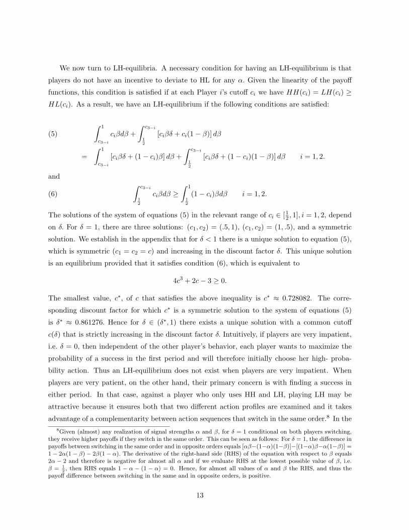
We now turn to LH-equilibria. A necessary condition for having an LH-equilibrium is that

players do not have an incentive to deviate to HL for any α. Given the linearity of the payoff

functions, this condition is satisfied if at each Player i’s cutoff ci we have HH(ci) = LH(ci) ≥

HL(ci). As a result, we have an LH-equilibrium if the following conditions are satisfied:

∫ 1

c3−i

ciβdβ +

∫ c3−i

12

[ciβδ + ci(1− β)] dβ(5)

=

∫ 1

c3−i

[ciβδ + (1− ci)β] dβ +

∫ c3−i

12

[ciβδ + (1− ci)(1− β)] dβ i = 1, 2.

and

(6)

∫ c3−i

12

ciβdβ ≥

∫ 1

12

(1− ci)βdβ i = 1, 2.

The solutions of the system of equations (5) in the relevant range of ci ∈ [12 , 1], i = 1, 2, depend

on δ. For δ = 1, there are three solutions: (c1, c2) = (.5, 1), (c1, c2) = (1, .5), and a symmetric

solution. We establish in the appendix that for δ < 1 there is a unique solution to equation (5),

which is symmetric (c1 = c2 = c) and increasing in the discount factor δ. This unique solution

is an equilibrium provided that it satisfies condition (6), which is equivalent to

4c3 + 2c− 3 ≥ 0.

The smallest value, c∗, of c that satisfies the above inequality is c∗ ≈ 0.728082. The corre-

sponding discount factor for which c∗ is a symmetric solution to the system of equations (5)

is δ∗ ≈ 0.861276. Hence for δ ∈ (δ∗, 1) there exists a unique solution with a common cutoff

c(δ) that is strictly increasing in the discount factor δ. Intuitively, if players are very impatient,

i.e. δ = 0, then independent of the other player’s behavior, each player wants to maximize the

probability of a success in the first period and will therefore initially choose her high- proba-

bility action. Thus an LH-equilibrium does not exist when players are very impatient. When

players are very patient, on the other hand, their primary concern is with finding a success in

either period. In that case, against a player who only uses HH and LH, playing LH may be

attractive because it ensures both that two different action profiles are examined and it takes

advantage of a complementarity between action sequences that switch in the same order.8 In the

8Given (almost) any realization of signal strengths α and β, for δ = 1 conditional on both players switching,they receive higher payoffs if they switch in the same order. This can be seen as follows: For δ = 1, the difference inpayoffs between switching in the same order and in opposite orders equals [αβ−(1−α)(1−β)]−[(1−α)β−α(1−β)] =1− 2α(1− β)− 2β(1− α). The derivative of the right-hand side (RHS) of the equation with respect to β equals2α − 2 and therefore is negative for almost all α and if we evaluate RHS at the lowest possible value of β, i.e.β = 1

2, then RHS equals 1 − α − (1 − α) = 0. Hence, for almost all values of α and β the RHS, and thus the

payoff difference between switching in the same and in opposite orders, is positive.

13

limit when players are perfectly patient (δ = 1), the cutoff converges to that of the symmetric

HL-equilibrium, since perfectly patient players care about which cells are investigated, but not

in which order.

The next proposition summarizes our discussion thus far:

Proposition 1 The entire set of equilibria in which neither player is indifferent between HL

and LH for all signal realizations has the following form: For all δ ∈ (0, 1), there exists a

symmetric HL-equilibrium with common cutoff c ≈ 0.760935 and there exist two asymmetric

HL-equilibria with cutoffs (c1, c2) = (.5, 1) and (c1, c2) = (1, .5), respectively. Furthermore, there

is a critical discount factor δ∗ ≈ 0.861276 such that for all δ ∈ (δ∗, 1) there exists a symmetric

LH-equilibrium with common cutoff c(δ), which is strictly increasing in δ, where c(δ∗) ≈ 0.728082

and c(1) ≈ 0.760935. Conversely, no LH-equilibrium exists for δ < δ∗.

Proposition 1 completely characterizes the set of equilibria that satisfy the condition HL(1) 6=

LH(1) for both players. Under some conditions, there also exist equilibria with HL(1) = LH(1)

for at least one player. (We construct such equilibria in the appendix.) Since in these equilibria

one or both of the players are indifferent between HL and LH over a range of signal strengths

that has positive probability, we call these IN-equilibria. In an IN-equilibrium at least one of the

players either randomizes between LH and HL over some range of signal strengths or one can

partition a subset of the set of possible signal strengths into sets where she either plays LH or HL.

In either case, IN-equilibria can be ignored in the search for optimal strategy profiles. Players

would be better off if both players switched to playing HL over the relevant range: If a single

player switches payoffs are not affected because of indifference; if then the other player switches

as well payoffs strictly increase because HL is strictly better than LH against HL. To find the

optimal equilibrium, we thus only have to compare the payoffs from the equilibria characterized

in Proposition 1. For each player, all of these equilibria are simple in the sense that they assign

a particular action sequence to a convex subset of her signal space (here the unit interval).9

Furthermore, when considering the equilibria of Proposition 1, we can immediately rule out

that an LH-equilibrium is optimal: To see this, simply change both players’ strategies to HL-

strategies, without changing the cutoff. Under the original strategies, there are three possible

events, each arising with strictly positive probability: Both players follow an HH-sequence; both

follow an LH sequence; and, one follows an LH-sequence while the other follows an HH sequence.

Clearly LH is not optimal against HH and therefore in this instance the new strategy yields a

strict improvement. Also, both players following HL rather than LH yields a strict improvement

9Below we will illustrate that this feature of optimal equilibria generalizes to other distributions and anarbitrary number of players and periods.

14

for impatient players. Thus in two events there is a strict payoff improvement, in the remaining

event payoffs are unaffected, and all three events have strictly positive probability.

It is, however, not immediately clear whether to prefer the symmetric HL-equilibrium or

the asymmetric HL-equilibria. In either, there is positive probability that profiles are searched

in the wrong order. The symmetric equilibrium makes the second-period switching probability

sensitive to a player’s signal, which seems sensible. At the same time, it introduces an additional

possible source of inefficiency. Players may not succeed in the first round despite having signals

so strong that they do not switch in the second round. In that case, they inefficiently search

only one of the available profiles.

It would be a straightforward matter to calculate and compare payoffs from symmetric and

asymmetric equilibria directly. We will follow a different line of reasoning, whose logic parallels

the one we use in Lemma 1 and Proposition 12 for the general model. Start with the asymmetric

HL-equilibrium in which c1 = 12 and c2 = 1. Consider the (informationally-constrained) social

planner who raises c1 from 12 and lowers c2 from 1 by the same small amount γ. The social

planner thus induces Player 1 to switch rather than to stick with her high-probability action

whenever both of her actions are (approximately) equally promising and at the same time induces

Player 2 to stick to her high-probability action whenever she is (approximately) certain that her

high-probability action is correct. This does not change first-period actions or payoffs, and the

second-period payoff as a function of γ is proportional to

π(γ) =

∫ 1−γ

12

∫ 12+γ

12

(1− α)(1− β)dαdβ +

∫ 1

1−γ

∫ 12+γ

12

(1− α)βdαdβ +

∫ 1−γ

12

∫ 1

12+γ

α(1− β)dαdβ.

It is straightforward to check that ∂π(γ)∂γ

∣∣∣γ=0

= 0 and ∂2π(γ)∂γ2

∣∣∣γ=0

> 0. Hence, the social planer

can improve on the two asymmetric equilibria. In common interest games an optimal strategy

profile is a Nash equilibrium, and we prove that an optimal strategy exists for our general model

below. This implies that for any arbitrary strategy profile σ, either σ is an equilibrium or there

exists an equilibrium σ∗ with ui(σ∗) > ui(σ) for i = 1, 2. Thus the pair of cutoff strategy profiles

with cutoffs c1 = 1/2 + γ and c2 = 1 − γ with an appropriately small value of γ either is an

equilibrium or there exists an equilibrium that strictly dominates it. Furthermore, an optimal

strategy profile must be one of the partition-equilibria characterized in Proposition 1. Therefore,

we have the following observation:

Proposition 2 For any δ ∈ (0, 1), in the two-player two-action two-period game with signals

that are independently and uniformly distributed, the symmetric HL-equilibrium is the optimal

15

equilibrium and at the same time the optimal strategy that an informationally-constrained social

planner would implement.

The example nicely illustrates that routines are suboptimal with fully rational players. This

raises the question why players would select such a Pareto-dominated equilibrium. Furthermore,

in the example there is no given routine that stands out, which leads to the further question of

how players would select a particular routine. We informally think of routines as being selected

by the management of the organization, which makes recommendation to the players of how to

behave. This, in turn, raises the question under what circumstance management would want to

select a problem-solving routine. The following example highlights that routines can be optimal

if agents are not fully rational. We begin by arguing that routines can be optimal when agents

are overconfident.

Suppose that a player interprets her signal as having a first-order statistic of (1 − x)α + x,

where x ∈ (0, 1). In this stylized example, x is a measure of a player’s overconfidence. As

x approaches 1, a player always believes with (almost certainty) to know what her correct

action is while the true probability is still uniformly distributed. For the sake of the example,

suppose both players are equally overconfident (have the same x) and consider the payoff of a

symmetric HL-type equilibrium in which players are meant to play HH when very confident and

HL otherwise. In particular, we suppose that an overconfident player correctly predicts for what

signals her fellow team member switches and consider the true signal at which she is indifferent

between switching and not switching. That is for any given true cutoff signal c3−i of her fellow

team member, a player with a perceived signal ci ≡ (1 − x)ci + x must be indifferent between

switching and not switching. Now replacing ci with the perceived signal (1−x)ci+x in Equation

4, shows that if Player i becomes extremely overconfident(x → 1), then her true cutoff signal

approaches (1/2) for any c3−i > 1/2. This implies that in the symmetric equilibrium as both

players become extremely overconfident (x → 1), the true equilibrium cutoff signal approaches

1/2.10 Intuitively, as long as there is a small probability of the other player switching, an

extremely overconfident player will be to reluctant to switch herself, and as her overconfidence

gets extreme (x approaches 1) she will almost never do so.

Clearly, however, as the common cutoff c → 1/2 the players’ payoff is less than in a routine.

Observe also that routines remain equilibria when players are overconfident. Even if Player

i is extremely confident that she knows what action is correct, if Player j never switches it is

10Formally, take any sequence of equilibrium cutoffs c(x) as x → 1. This sequence must have a convergentsubsequence. Suppose the convergent subsequence converges to some cutoff c > 1/2. Then for any ǫ > 0, thereexists an x such that for all x > x, c(x) ∈ (c− ǫ, c+ ǫ). This however contradicts the above established fact thatfor any c > 1/2, the cutoff signal her team member responds with goes to 1/2.

16

optimal to switch for Player i. Hence, in our example, when players are sufficiently overconfident

it becomes strictly optimal for the management to implement a routine, and the payoffs of the

routine are fully robust to players’ overconfidence. Indeed, straightforward calculations reveal

that for all x > .374 routines perform better than the symmetric overconfident HL-equilibrium.

We emphasize that overconfidence can justify the use of routines in

Proposition 3 For any δ ∈ (0, 1), in the two-player two-action two-period game with signals

that are independently and uniformly distributed, if players are sufficiently overconfident, then

the payoff of an ordinal equilibrium is higher than that of the overconfident symmetric HL-

equilibrium.

Routines are also robust to other types of biases documented and modeled in behavioral

economics. For example, suppose agents are strategically naive in the sense that they play cursed

equilibria. In a fully cursed equilibrium, each player best responds to the actual distribution

of actions sequences by the other player but fails to take into account how this distribution of

action sequences depends on the other player’s type. In an ordinal equilibrium, one player—say

1—always switches. It is then clearly optimal for Player 2 to always select her high probability

action even if not realizing that Player 1 switches from her high to her low-probability action.

Similarly, given that Player 2 does not switch, it is clearly optimal for Player 1 to do so. Hence

routines are fully cursed equilibria, and in this sense robust to strategic naivete of team members.

In contrast, the optimal equilibrium is not robust to such strategic naivete.

To see this, consider a symmetric fully-cursed equilibrium in which agents play HH when

having high signals and HL when having a low signal. In such a symmetric fully cursed equi-

librium with cutoff first-order statistic c, Player 2 switches with probability 2(c− (1/2)). Given

this behavior, a fully cursed Player 1 is indifferent between switching and not switching when

having a first-order statistic α if

(7) α

[∫ 1

0xdx

]

+ δα2

(

c−1

2

)[∫ 1

0xdx

]

= α

[∫ 1

0xdx

]

+ δ(1− α)

[∫ 1

0xdx

]

.

Furthermore, using that in a symmetric equilibrium α = c, the fully cursed equilibrium cutoff

satisfies: 2c2 − 1 = 0, so that the common cursed cutoff is equal to√

1/2. Now calculating

the true payoff when players use the above cutoff for δ = 1 shows that the expected payoff is

0.753 while the payoff of the ordinal equilibria is 0.75. In our example, thus, lack of strategic

sophistication severely reduces the benefits of optimal equilibria over routines—although in

this specific case not completely eliminating it. It is natural to also consider teams in which

members exhibit some combination of cursedness and overconfidence, or are unsure about either

17

the cursedness or overconfidence of fellow team members. We highlight in the next section that

routines are fully robust to relaxing the rationality constraint simultaneously in these directions.

4 The General Model

One can think of our model as a formal representation of the following stylized “safe problem”:

A group of individuals wants to open a safe. Each of them has access to a separate dial in an

isolated room. There is a single combination of dial settings that will open the safe. The group

repeatedly tries out different combinations. It is impossible to communicate or to observe the

actions of other group members. Initially, each individual privately and independently receives

a signal that indicates for each of her dial settings the probability of it being correct, i.e. being

part of the combination that will open the safe. The probability that any given combination is

correct is the product of the corresponding signals.

Each Player i out of a finite number I of players has a finite set of actions Ai that has

cardinality mi; we will slightly abuse notation by using I to denote both the set of players and

its cardinality. A := ×Ii=1Ai denotes the set of action profiles. A typical element of Ai is denoted

ai and we write a = (ai, a−i) ∈ A for a typical action profile. There is a single success profile

a∗ ∈ A with a common positive payoff u(a∗) = 1, and the common payoff from any profile a 6= a∗

equals u(a) = 0. The location of the success profile a∗ is randomly chosen from a distribution

ω ∈ Ω := ∆(A) over the set of all action profiles. The distribution ω itself is randomly drawn

from a distribution F ∈ ∆(∆(A)), the set of distributions over distributions of success profiles.

This permits us to express the idea that players are not only uncertain about the location of

the success profile, but also that each player has some information regarding the location that is

unknown to others. Formally, after ω is chosen, each Player i learns ωi, the marginal distribution

over Player i’s actions. Thus, if ω(a) denotes the probability that ω assigns to the profile a being

the success profile, ωi(aij) =∑

j1,...,ji−1,ji+1,...,jnω(a1j1 , . . . aij . . . anjn) is the probability that a

success requires Player i to take action aij . Denote the set of Player i’s marginal distributions

ωi by Ωi.

We make two assumptions that limit how much players can infer about the signals of others

from their own signals. We assume action independence, which requires that each ω in the

support of F be the product of its marginals, i.e. ω = ΠIi=1ωi. Furthermore, we require signal

independence, which requires that F is the product of its marginals, Fi, i.e. F (ω) = ΠIi=1Fi(ωi).

11

Upon observing her signal a player therefore does not revise her belief about how confident other

players are about which of their actions are required for a success profile.

11We discuss possible consequences of violations of these assumptions in the Appendix.

18

Players choose actions in each of T < ∞ periods, unless they find the success profile, at

which point the game ends immediately. Players do not observe the actions of other players.

Therefore a player’s strategy conditions only on the history of her own actions. Denote the

action taken by Player i in period t by ati. Then Player i’s action history at the beginning of

period t is hit := (a0, a1i , . . . , at−1i ), where a0 is an auxiliary action that initializes the game. We

let ht = (h1t, . . . , hIt) denote the period-t action history of all players. The set of all period-t

action histories of Player i is denoted Hit, where we adopt the convention that Hi1 = a0.

The set of period-t action histories of all players is Ht and the set of all action histories of

all players is H := ∪Tt=1Ht. A (pure) strategy of Player i is a function si : Hit × Ωi → Ai

and we use s to denote a profile of pure strategies. For any pure strategy profile s and signal

vector ω, let at(s, ω) denote the profile of actions that is induced in period t. Similarly, define

At(s, ω) := a ∈ A|aτ (s, ω) = a for some τ ≤ t as the set of all profiles that the strategy s

induces before period t+ 1 when the signal realization is ω. A behaviorally mixed strategies σi

for Player i is a (measurable) function σi : Hit × Ωi → ∆(Ai). We use ΣTi to refer to the set of

such strategies in the T -period game. ΣT := ×i∈IΣTi is the set of mixed strategy profiles in the

T -period game. Players discount future payoffs with a common factor δ ∈ (0, 1). Thus, if t∗ is

the first period in which the success profile a∗ is played, the common payoff equals δt∗−1; if the

success profile is never played the common payoff is zero.

We will now formally describe payoffs. For that purpose define a 6∈ ht as the event that

action profile a has not occurred in history ht. Furthermore let the probability of reaching the

initial history Prob(h1|σ, ω, a) = 1 and for t > 1, with ht = (ht−1, a′) denoting the action history

ht−1 followed by the action profile a′, recursively define the probability of reaching history ht

given σ, ω and given that a is the success profile through

Prob(ht|σ, ω, a) := 1a 6∈ht−1

∏

i∈I

σi(a′i|hi,t−1, ωi)Prob(ht−1|σ, ω, a).

Then expected payoffs from strategy profile σ are given by∫

ω∈Ω

∑

a∈A

∑

ht∈H

δt−1∏

i∈I

σi(ai|hi,t, ωi)Prob(ht|σ, ω, a)ω(a)dF (ω),

where∏

i∈I σi(ai|hi,t, ωi)Prob(ht|σ, ω, a) denotes the (unconditional) probability that action pro-

file a is played following history ht and ω(a) is the probability that a is the success profile. We will

denote the expected payoff from strategy profile σ by π(σ) and Player i’s expected payoff from

strategy profile σ conditional on having observed signal ωi by πi(σ;ωi). Observe that expected

payoffs are well-defined since ∆(A) is a finite-dimensional unit simplex, and F is a distribution

over this simplex. For simplicity, we assume throughout the paper that F has full support on

19

∆(A). The timing of the game is as follows: (1) Nature draws a distribution ω ∈ ∆(A) from the

distribution F. (2) Each player receives a signal ωi. (3) The success profile is drawn from the

realized distribution ω. (4) Players start choosing actions.

One of our objectives in this paper is to demonstrate that routines are often suboptimal,

and hence we compare them to optimal strategies. Regarding optimal strategies, some facts are

worth noting. First, since we are studying common interest games, i.e. the payoff functions of the

players coincide, there is a simple relation between optimality and (Bayesian Nash) equilibrium.

An optimal strategy profile must be a Nash equilibrium since all players have a common payoff

and if there were a profitable deviation for one player, then a higher common payoff would be

achievable, contradicting optimality.12 Second, as long as an optimal strategy profile exists,

this observation has the following useful corollary: any equilibrium that is payoff-dominated by

some strategy is also payoff-dominated by an equilibrium strategy. We use this fact repeatedly

throughout.

The third noteworthy fact is that optimality implies sequential rationality in common interest

games. Specifically, any optimal outcome of a common interest game can be supported by a

strategy profile σ that is an essentially perfect Bayesian equilibrium (EPBE) (see Blume and

Heidhues [2006] for a the formal definition and detailed discussion of EPBE)13, i.e. one can

partition the set of all histories into relevant and irrelevant histories so that σ is optimal after

all relevant histories regardless of play after irrelevant histories. In general games it is frequently

the case that Nash equilibria are supported by specific behavior off the path of play, which may

not be sequentially rational. In an optimal strategy profile of a common-interest game, however,

following the prescribed behavior on the path of play is optimal independent of what players do

off the path of play. This can be seen as follows. Classify any history off the path of play of an

optimal profile σ as irrelevant and any other history as relevant. Now suppose that there is a

partial profile σ−i that agrees with σ−i on the path of play and a deviation σ′i of Player i from σi

that is profitable against σ−i. Then, since we have a common interest game, the strategy profile

(σ′i, σ−i) yields a higher payoff for all players than σ, which contradicts optimality of σ.

Below, after formally introducing and characterizing them, we also show that routines are

sequentially rational by proving that any ordinal equilibrium outcome in our setting can be

supported by an EPBE.

12This is also used in Alpern [2002], Crawford and Haller [1990], and McLennan [1998].13In finite games the outcomes that are supported by perfect Bayesian equilibria coincide with those supported

by EPBEa. The use of EPBE, however, allows one to focus on the economically relevant aspects of the sequentialrationally requirement because it does not require one to specify behavior after irrelevant histories, which althougheconomically irrelevant can be technically challenging. Furthermore, if following irrelevant histories continuationequilibria do not exist in infinite games, EPBE is a superior solution concept.

20

5 Organizational Routines

5.1 Characterization of Routines

In this section we identify and characterize a class of equilibria that have a natural interpretation

as organizational routines. In these ordinal equilibria players use strategies that condition only

on the rank order of signals not their value, which implies that independent of the concrete

signal realization team members always switch actions in a pre-specified order, thereby inducing

the common pattern of behavior that we interpret as a particular problem-solving routine.

a1,1

a1,2

a2,1 a2,2 a2,3

1 2 3

4 5 6

Figure 1

For an informal introduction of these routines consider, for example, the matrix of action

profiles in the stage game in Figure 1. In the figure ai,j denotes the j-th action of Player i,

wlog ranked in the order of the corresponding signals, i.e. if we denote by αi,j the probability

that the j-th action of Player i is part of a success profile, then αi,j ≥ αi,j+1 for all i and j. For

convenience, the six action profiles have been numbered. Then there is an ordinal equilibrium

in which the profile labeled t is played in period t = 1, ..., 6. In this equilibrium, Player 1 plays

her most probable action in the first three periods during which Player 2 begins with her most

likely action, then tries the next most likely action, and finally attempts her least likely action.

Thereafter Player 1 switches to her least likely action and Player 2 repeats the previous sequence

of actions. Taking the action sequence of the other player as given, in each period both players

select the action that is most likely to lead to a success. On the other hand, there is no ordinal

equilibrium in which players play the sequence of profiles 1, 3, 2, 4, 5, 6: given that Player 1 is

playing her most probable action in the first three periods, Player 2 can deviate from such a

candidate equilibrium and in the first three periods select her action in the order of likelihood

of leading to a success, thereby inducing the profile 1, 2, 3, 4, 5, 6, which yields a higher payoff.

This discussion suggest that a defining characteristic of ordinal equilibria is that each player

in every period selects the action that is most likely to lead to a success. Propositions 4 and

5 indeed show that all ordinal equilibria are characterized by players selecting such maximal

actions—which are precisely defined below—in every period. This, however, gives rise to a rich

21

class of equilibria including some counterintuitive incomplete search equilibria that nevertheless

satisfy (the spirit of) trembling-hand perfection as we illustrate below. Proposition 6 establishes

that the entire class of ordinal equilibria is sequentially rational, and Proposition 7 specifies the

optimal ordinal equilibrium or optimal routine.

We now turn to formally introducing routines. For tie-breaking purposes, it is convenient to

introduce a provisional ranking of Player i’s actions, where all provisional rankings have equal

probability and Player i learns the provisional ranking at the same time as she learns ωi. Using

this provisional ranking to break ties where necessary, for any signal ωi, we can generate a vector

r(ωi) that ranks each of Player i’s actions aij , from the highest to the lowest probability of that

action being required for a success. A strategy is ordinal if it only conditions on whether an

action is more likely then another—i.e. has a higher rank—and not on how much more likely a

particular action is. More precisely, a strategy σi of Player i is ordinal if there exists a function

σi such that σi(hit, ωi) = σi(hit, r(ωi)) for all hit ∈ Hit and all ωi ∈ Ωi. A profile σ is ordinal if

it is composed of ordinal strategies; otherwise, it is cardinal.

For any action history ht define A(ht) := a ∈ A|a ∈ ht as the set of all action profiles that

have occurred before time t in history ht. Given a strategy profile σ and any private history

(ωi, hit) that is consistent with that profile (i.e. for which hit has positive probability given σ

and ωi), let At−i(σ−i, hit, ωi) = a−i ∈ A−i|Prob(a

t−i = a−i|hit, ωi, σ−i) > 0 be the set of partial

profiles that have positive probability in period t given Player i’s information σ−i, hit, and ωi.

For a strategy profile σ and any private history (ωi, hit) that is consistent with that profile, we say

that the action aij is promising for Player i provided that given her information (σ−i, hit, ωi)

there is positive probability that it leads to a success.14 An action aij is rank-dominated for

a strategy profile σ following history (ωi, hit) if there exists a promising action aij′ such that

ωij′ > ωij . An action aij is maximal for a strategy profile σ following history (ωi, hit) if it is

promising and rank–undominated or if no promising action exists. Roughly speaking, given the

behavior of all other players, a maximal action has the highest probability of finding a success

in the current period. We begin by observing that players must choose maximal actions on the

path of play of any ordinal equilibrium.

Proposition 4 If a profile of ordinal strategies σ is an equilibrium, then for every ωi and every

history of actions hit that has positive probability given σ and ωi, Player i plays a maximal

action.

14Formally, thus, given a strategy profile σ and a private history (ωi, hit) that is consistent with that pro-file, the action aij is promising for Player i if Prob

(aij , a−i) 6∈ A(ht) ∩ (aij , a−i)|a−i ∈ At−i(σ−i, hit, ωi)|

ωi, hit, σ−i > 0.

22

The proof of the proposition proceeds by noting that whenever there is a period in which

Player i plays a non-maximal action, there is a signal realization ωi that puts zero probability of

success on all actions below this maximal action and positive success probability on the maximal

action. In this case, however, Player i can profitably deviate by playing the maximal action in

that period and thereby increasing the probability of success in that period. This either moves

success probability forward—if this cell was going to be investigated in a later period anyhow—

or simply increases the probability of success and hence contradicts that playing a non-maximal

action can be optimal for all signal realizations in a candidate ordinal equilibrium.

Conversely, we observe next that if players choose maximal actions along the path of play

of an ordinal strategy profile, then this strategy profile is an equilibrium. To this end, we say

that Player i’s strategy σi is maximal against the partial profile σ−i if it prescribes a maximal

action for Player i for every signal ωi and every action history hit that has positive probability

given σ and ωi. A strategy profile σ is maximal if σi is maximal against σ−i for all players i.

Proposition 5 If a profile σ of ordinal strategies is maximal, then it is an equilibrium.

The proof proceeds in four steps: (1) We show that if a profile of ordinal strategies σ is

maximal, then for every Player j every pure strategy in the support of σj induces the same

actions in periods in which there is a positive probability of a success. (2) We conclude from (1)

that if σi is maximal against σ−i, then it is maximal against all s−i in the support of σ−i. (3)

We show that if σi is maximal against a pure strategy profile s−i then it is a best reply against

that profile. And finally, (4) we appeal to the fact that if σi is a best reply against every s−i in

the support of σ−i, then it is a best reply against σ−i itself.

Propositions 4 and 5 show that ordinal equilibria have a simple structure: Actions profiles

that are higher (in a vector sense based on the players’ signal) are tried before lower profiles.

There is substantial multiplicity of such equilibria because the ordering is not complete and

therefore coordination on an ordinal equilibria is difficult. If, however, coordination on an ordinal

equilibrium is achieved by some mechanism this equilibrium will prove remarkably robust.

We now argue that every ordinal equilibrium outcome is sequentially rational by proving

that it can be supported by an EPBE. For any ordinal equilibrium profile σ classify histories

on the path of play as relevant and all other histories as irrelevant. Take any strategy profile

σ that coincides with σ on the path of play. We need to argue that playing according to σi

remains a best response to σ−i for any history on the path of play. In an ordinal equilibrium

there exists a commonly known first period τ with the property that either a success is achieved

with probability one in a period t ≤ τ or τ is the final period. Because a deviation of Player

23

i is not detected prior to period τ , it does not change the behavior of all other players in any

period t ≤ τ . Since given the behavior of all other players, Player i plays a maximal action in

every period t ≤ τ , a deviation by i cannot increase her expected payoff conditional on finding

a success prior to τ , and it must lower it whenever a success is found after period τ . Hence, it

remains optimal to play according to σi on the path of play. We thus have:

Proposition 6 Any ordinal equilibrium outcome can be supported by an EPBE and thus is

sequentially rational.

Observe that the equilibria characterized in Propositions 4 and 5 include (i) equilibria in

which all profiles are examined without repetition, (ii) equilibria in which search stops before all

profiles have been examined, and (iii) infinitely many Pareto-ranked equilibria in which search

is temporarily suspended and then resumed. Reconsider the example illustrated in in Figure

1, where ai,j denotes the j-th action of Player i, and wlog we ranked these actions in the order

of the corresponding signals. Then, (i) there is an equilibrium in which the profile labeled t is

played in period t = 1, . . . , 6, (ii) another equilibrium in which the profile labeled t is played in

period t = 1, . . . , 4 after which profile 1 is played forever, and (iii), for any k with k > 0 and

k < T − 4 there is an equilibrium in which the profile labeled t is played in period t = 1, . . . , 4

after which profile 1 is played for k periods followed by play of profiles 5 and 6.

Somewhat counter-intuitively, such ordinal equilibria in which search ends prematurely, or

is temporarily suspended, survive elimination of dominated strategies. To see this, return to

our example with two players, two actions, a uniform signal distribution, but now with T ≥ 4

periods. For the row player let H (L) denote taking the high (low) probability action, regardless

of the value of the signal. For the column player, use lower case letters, i.e. h and l, to describe

the same behavior. Then G1G2 . . . GT with Gt ∈ H,L is the strategy of the row player that

prescribes taking the action Gt in period t regardless of the value of the signal, and similarly for

the column player.

Suppose that the row player believes that the column player uses the strategy hlhhhhh . . . h

with probability 1 − ǫ and the strategies lllhl . . . l, llllhl . . . l, . . . , llll . . . lhl and llll . . . llh each

with probability ǫT−3 . Then the strategy HHLH . . .H is a unique best reply for almost every

realization of the row player’s signal (and a best reply for every signal realization). This implies

that HHLH . . .H is an undominated strategy for the row player. By an analogous argument

it follows that hlh . . . h is an undominated strategy for the column player. Hence, we have an

equilibrium in undominated strategies in which search terminates after the third period, even if

until that point there has been no success and there are arbitrarily many future search periods

left.

24

If we discretize the game by considering signal distributions with a finite support, we have a

finite game and can check equilibria for trembling-hand perfection. It is well known that in finite

two-player games the set of (normal form) perfect equilibria coincides with the set of equilibria

in undominated strategies. As a consequence, in the discrete approximation of our game the

equilibrium (HHLH . . .H, hlh . . . h) is (normal form) perfect. In this sense, the equilibrium is

robust and similar constructions can be found in the case with more players and or actions.

Although even these clearly suboptimal equilibria satisfy the spirit of trembling-hand per-

fection, in our interpretation of routines as being selected by management, it is implausible that

such routines would be selected. Management would clearly prefer to select an optimal routine

to an obviously suboptimal one and hence we now show that an optimal routine exists and

characterize it.

Denote the random variable that is Player i’s signal by ωi, to distinguish it from the signal

realization ωi, and let ωi(n) stand for the nth (highest) order statistic of the random vector

ωi. Define ωi(n) as the expectation E[ωi(n)] of the nth order statistic of Player i’s signal. For

every realization ωi, use ai(ni)(ωi) to denote the action of player i with the nith highest signal

according to ωi. For any i and n, let ai(n) denote the rule of playing the nth highest action for

any signal realization ωi. Refer to the rule ai(n) as Player i’s nth rank-labeled action and to

every (a1(n1), a2(n2), . . . , aI(nI)) as a rank-labeled action profile.

Proposition 7 An optimal ordinal equilibrium exists and in any optimal ordinal equilibrium

agents play a sequence of rank-labeled action profiles in the order of their ex ante success prob-

ability without repetition.

Conceptually, finding an optimal routine is simple. For each team member determine the

expected values for the order statistics of that team member’s signal vector; for each profile

of such expectations multiply these expected values; and, play profiles in decreasing order of

the magnitude of these products. Note however that while routines are easy to find and do

not depend on detailed knowledge of signal distributions, finding an optimal routine may be

computationally burdensome and optimality will generally depend on which distributions signals

are drawn from.

5.2 Robustness of Routines

Having specified the class of ordinal equilibria and found the optimal equilibrium in this class,

we turn to highlight the robustness of these routine equilibria. Loosely speaking, we begin by

showing that the class of ordinal equilibria coincides with the class of ex post equilibria. An

25

equilibrium is an ex post equilibrium if each player’s strategy remains a best response even after

learning the other players’ private information. Since ex post equilibria induce best replies for

every signal distribution, they do not depend on the distribution that generates players’ signals

or the beliefs that players have about how signals are generated. Another consequence in our

setting is that an outsider without knowledge about how signals are generated or how players

form their beliefs could step in and help coordination by suggesting an ordinal equilibrium profile.

That ordinal equilibria are ex post is intuitive given the fact that our informal discussion at the

beginning of this section made no references to the underlying signal distribution; once I know

that one of my partners switches after the first period with probability one, it is a best response

for everyone else to stick to their high probability action independent of the signal realizations;

and once everyone else does not switch, is is clearly a best response for the designated player to

switch independent of her and other players’ private information. Similarly, in later periods—as

long as they are promising—exactly one player will switch to a lower probability action and

given the behavior of other players, this is optimal independent of the signal realization. But

it is worth emphasizing that we also show that basically only ordinal equilibria are ex post.

Hence a management that wants a robust solution with respect to the underlying distribution

needs to select a routine. Finally, in Proposition 10 we show that routines are also hyper-

cursed equilibria: they are robust to a wide variety of incorrect beliefs by the team members.

A management having to deal with less than perfectly rational agents may thus benefit from

selecting routines, which are robust to a variety of behavioral biases documented in the literature

on behavioral economics.

5.2.1 Routines are ex post Equilibria

The following proposition, which focuses on pure strategies, establishes a simple and clean

equivalence of the set of ordinal and the set of ex post equilibria. We discuss more general

results for mixed strategies below (Proposition 9).

Proposition 8 The set of pure-strategy ex post equilibria coincides with the set of pure-strategy

ordinal equilibria.

It is straightforward to see that every ordinal equilibrium σ is an ex post equilibrium, even

if we allow for mixed strategies: According to Proposition 4, in an ordinal equilibrium in every

period in which there is a positive probability of a success, a player plays a maximal action.

The property of an action being maximal for Player i does not depend whether or not the

entire signal vector ω is known; i.e., an action that is maximal for Player i when ω−i is private

26

information remains maximal when ω−i is made public. Thus even when the signal vector ω is

publicly known there is no instantaneous gain from switching to a different action in any period

in which there is a positive probability of a success. Evidently, in periods in which there is no

positive probability of success, even with knowledge of ω−i, there is no instantaneous gain from

deviating from σ. Since actions are not observed, a player can also not hope to affect future play

of others by switching from a maximal to a non-maximal action. Therefore, it remains optimal

to maximize the instantaneous probability of success by taking a maximal action and hence σ

is an ex post equilibrium. The converse is established in the appendix.

Since ordinal equilibria are ex post even when we allow for mixed strategies, one may wonder

whether mixed-strategy ex post equilibria also coincide with ordinal equilibria. To understand

intuitively, why this is not the case reconsider the example illustrated in Figure 1. Then if

T = 6 there exists an ordinal equilibrium in which in periods t = 1, · · · , 5 the corresponding

action profile is played, so that on the path of play all but the a priori-least likely action profile

have been played prior to the final period. In the final period Player 1 plays her first action

(a1,1) while Player 2 randomizes (with any given probability) between the two more likely actions

(a2,1, a2,2); in this incomplete-search equilibrium no player can deviate in the final period and

induce a positive probability of success. Note also that this ordinal equilibrium is ex post,

which follows from the above arguments for the first 5 periods and the fact that independent of

the signal realization no player can induce a success in the final period. If this randomization

by Player 2, however, conditions on more than her ordinal ranking of signals, the resulting

equilibrium is not ordinal and yet ex post. What our next proposition establishes, is that ex post

equilibria differ from ordinal equilibria only with regard to such inconsequential randomization

in which players randomize between multiple maximal action—i.e. randomize in non-promising

periods. Thus, subject to this minor qualification, the behavior in ex post equilibria coincides

with that in ordinal equilibria: The set of (mixed-strategy) ex post equilibria share with ordinal

equilibria the property of inducing maximal actions in every period.

Proposition 9 In any ex post equilibrium every player plays a maximal action in every period.

Note that the above Propositions 7 and 9 imply that an optimal routine is also an optimal

ex post equilibrium, and that an optimal ex post equilibrium is a routine.

5.2.2 Robustness to Behavioral Biases

We now turn to illustrate the robustness of routines to behavioral biases, beginning with a

lack of strategic sophistication by players that is formally incorporated in the concept of cursed

27

equilibria. In a fully cursed equilibrium (Eyster and Rabin [2005]) every type of every player best

responds to the correct probability distribution over the other players’ actions that is induced by

their equilibrium strategies, but does not properly attribute these actions to the other players’

private information.15 To state this condition formally in our setting, we need to introduce some

notation: We denote a sequence of actions for Player i in the T -period game by λi. Given, a

signal profile ω, a profile λ of such action sequences induces an expected payoff ui(λ, ω). For any

strategy profile σ (with a slight abuse of notation) denote by σ−i(λ−i|ω−i) the probability with

which players other than i follow the partial profile of action sequences λ−i if their signals are

given by ω−i. Since σ−i(λ−i|ω−i) =∏

j 6=i σj(λj |ωj), it is measurable and thus we can define the

expected average play of others as

σ−i(λ−i|ωi) :=

∫

Ω−i

σ−i(λ−i|ω−i)dpi(ω−i|ωi),

where pi(·|ωi) is Player i’s posterior distribution over the other team members’ signals conditional

on her own. Then σ is a fully cursed equilibrium if for every i, ωi ∈ Ωi and every action sequence

λi ∈ supp[σi(·|ωi)],

λi ∈ argmaxλi

∫

Ω−i

∑

λ−i∈Λ−i

u(λ, ω)σ−i(λ−i|ωi)dpi(ω−i|ωi),

where u(λ, ω) denotes the (common) expected payoff if the signal realization is ω and players

follow the profile of action sequences λ. Note that because of signal independence in our case

pi(ω−i|ωi) = F−i(ω−i), and σ−i(λ−i|ωi) simplifies to

σ−i(λ−i) =∏

j 6=i

∫

Ωj

σj(λj |ωj)dFj(ωj).

While cursedness captures the idea that players underestimate the extent to which other

players’ actions depend on their information, our ordinal equilibria are robust to many other

biases in information processing. To illustrate this, we will considerably strengthen the cursed-

ness requirement in several dimensions, and show that pure-strategy ordinal equilibria satisfy

these conditions.

First, while cursedness requires a player to correctly predict the distribution of other players’

action sequences, we can relax this assumption and ask instead that the player merely correctly

predicts the support of the distribution. Formally, we strengthen the robustness requirement

by asking that σ satisfies the condition that for every Player i, own signal ωi ∈ Ωi, profile of

15As is well known, a fully cursed equilibrium corresponds to an analogy-based equilibrium (Jehiel [2005]) witha “private information analogy partition” (Jehiel and Koessler [2008])—i.e. a partition that groups together alltypes of other players.

28

other players’ action sequences λ−i ∈ ∪ω′

−isupp[σ−i(λ−i, ω

′−i)], and every own action sequence

λi ∈ supp[σi(·|ωi)]:

λi ∈ argmaxλi

u(λ, ω) ∀ ω−i.

We refer to any σ that has this property as a strongly cursed equilibrium. In a strongly

cursed equilibrium, a player must best respond to any action sequence played by others on the

path of play—independent of what the true type of other players is.16 It is thus robust to any

misperception of how other players’ equilibrium behavior depends on their information. For

example, the frequency with which a player thinks her partner’s play a given sequence need not

match this frequency in equilibrium. In our organizational interpretation in which a routine

is selected by a management that cannot observe the team members’ private information, this

requirement can also be interpreted as a weak-accountability condition in the sense that every

player believes that her fellow team members choose only action sequences that can be justified

in front of the management as being consistent with the management’s order for some possible

private signal realization.

Second, a player may also put positive weight on some action sequences that are not played in

equilibrium as long as she correctly predicts when other players switch between actions and when

previously chosen actions are repeated. As an example, think of a player who has three actions

of which the third action is always the least likely action. Consider a candidate equilibrium in a

two-period game in which she is meant to always play the most likely action. Then, for example,

we allow her partner to misperceive her behavior of not switching as always playing the third

action even though this is never the most likely action. To capture this formally, for any set Λ−i

of profiles of action sequences of other players use L(Λ−i) to denote the set that is obtained by

replacing any action sequence λk = (a1k, . . . aTk ) of any Player k 6= i by ℓ(λk) = (ℓ(a1k), . . . ℓ(a

Tk ))

where ℓ is any permutation of Player k’s set of actions Ak. Then we ask that σ satisfy the

condition that for every Player i, own signal ωi ∈ Ωi, λ−i ∈ L(

∪ω′

−isupp[σ−i(λ−i, ω

′−i)])

, and

every own action sequence λi ∈ supp[σi(·|ωi)]:

λi ∈ argmaxλi

u(λ, ω) ∀ ω−i.

Third, in addition to the above misperceptions of other players’ behaviors, we can allow

for a player to misinterpret her own signal as longs as the ranking of her own signals remains

16Strongly cursedness is a far stronger requirement as cursedness; for example in the standard independent-private value auction environments every Nash equilibrium is (fully) cursed but not necessarily strongly cursed.In the second-price independent private-value auction, the dominant strategy equilibrium is strongly cursed. Ingeneral, however, ex post equilibria need not be cursed and hence also not strongly cursed.

29

correct.17 For example, in a setting in which a player’s signals are the result of her ability

to understand and analyze the basic problem, overconfidence may result in her thinking that

the most likely action is part of a success profile with a higher than appropriate probability.

Similarly, if a player’s signal comes from repeatedly drawing from her signal distribution, the

belief-in-small-numbers bias may often lead to overconfidence. Whatever the exact driver of

incorrect own beliefs, a player will want to stick to the prescribed play, and in addition the true

expected payoffs of the ordinal equilibrium are unaffected by these biases.

Putting it all together, we say that an equilibrium σ is a hyper-cursed equilibrium if

for any Player i, true signal ωi and perceived own signal ωi that satisfies r(ωi) = r(ωi), λ−i ∈

L(

∪ω′

−isupp[σ−i(λ−i, ω

′−i)])

, and every own action sequence λi ∈ supp[σi(·|ωi)]:

λi ∈ argmaxλi

u(λ, (ωi, ω−i)) ∀ ω−i.

As our next result shows, in our setting pure-strategy ordinal equilibria are hyper-cursed

equilibria, as well as conventional Bayesian equilibria. Intuitively, what matters for a given

player is that the other players follow a particular pattern of play—i.e. of switching between

their various actions—and not on how the realization of this pattern depends on players’ signal

realizations. In terms of our example in Section 3, even if the other team member incorrectly

plays her low-probability action first, it is optimal to respond with playing one’s high-probability

action in the first period. Furthermore, if my fellow team member doesn’t switch, it is optimal

to switch in the second period and if my team member switches, it is optimal to keep playing

the high-probability action. And if players play a routine they only condition on the rank of

their signals and hence a misperception of their own signal strength is inconsequential as long

the ranking of own signals is unaffected. Thus routines are hyper cursed.

Proposition 10 Every pure-strategy ordinal equilibrium is hyper cursed.

We have the following trivial consequence:

Corollary 1 Every pure-strategy ordinal equilibrium is fully cursed.

We have focused here on an extreme version of strategic naivete, in addition allowing for

other misperceptions. The robustness of routines covers also different notions of partial strategic

naivete: it extends to partial cursedness as well as all versions of analogy-based equilibrium that

partition the type space of other players more finely than the trivial partition.18 This is easiest

17Observe that this notion is tailored to the specific problem we are considering and, in contrast to cursedness,not defined for games more generally.

18Jehiel and Koessler [2008], for example, introduce finer partitions of the type space in the Crawford and Sobel[1982] model of communication.

30

to see when introducing partial sophistication through finer partition in the above analogy-based

equilibrium concept: because all types of other players follow the same switching pattern in a

routine, and this switching pattern in itself determines a player’s best response, it does not

matter how a player groups the types of other players. Similarly, since all types of other players

have the same switching behavior, a partially cursed player correctly predicts the switching

behavior of others in a routine, and hence following the behavior prescribed by the routine

remains a best response.

5.3 Suboptimality of Routines

Having characterized routines and shown that their robustness generalizes from the example

of Section 3 to our entire class of games, we now turn to lessons on optimal equilibria that

generalize from the example. We demonstrate that: (1) it is impossible to implement ex post

optimal search; (2) optimal equilibria exist and have an intuitive form—they partition the signal

space into convex sets; and (3) typically optimal equilibria are cardinal, i.e. players condition

on their signal strength in addition to the ranking of signals. Thus, the robustness of (optimal)

routines comes typically at the cost of being a suboptimal equilibrium.

The impossibility of ex post-optimal search is a simple consequence of the fact that the

knowledge required to implement it is distributed across players. Ex post-optimal search would

require that players calculate the success probability of each action profile conditional on their

joint information and then try action profiles in declining order of these probabilities. To see

that this is not an equilibrium strategy with the available information, note that for almost

any signal vector ωi of Player i there exists a positive probability set of signal vectors of others

players such that the full-information optimal strategy has Player i change her action from

period one to period two. At the same time, for the same signal ωi of player i, there is a positive

probability set of signal vectors of other players for which the full-information optimal strategy

prescribes that Player i does not change her action between periods one and period two. This

behavior cannot be achieved in equilibrium since Player i’s behavior can only depend on her

own information

Given that ex post-optimal search is infeasible, the next question is how well one can do

while respecting the players’ informational constraints. In order to address this question, we

first note that the sets of optimal and of Nash equilibrium profiles can be analyzed in terms of

mappings from signals to distributions over action sequences. Since Player i has mi actions, she

can follow one of(mi)T

possible action sequences in the T -period game. We denote a typical

action sequence of this kind for Player i by λi and the set of such action sequences for Player

31

i by Λi. We show in the appendix that in the present environment the sets of optimal and of

Nash equilibrium profiles can be fully characterized in terms of the action-sequence mappings

χi : Ωi → ∆(Λi). This is a consequence of our assumption that players cannot observe and

therefore cannot condition their behavior on each others’ actions.

Every strategy σi of Player i induces a mapping χi|σi : Ωi → ∆(Λi) from signals into

distributions over action sequences. Strategies are particularly simple if they are pure and

the induced action sequence mappings are measurable with respect to a finite partition. This

motivates the following definition:

Definition 1 If there exists a finite partition P of the signal space of Player i such that the

action-equence mapping χi|σi : Ωi → ∆(Λi) is measurable with respect to P, then σi is a parti-

tion strategy with respect to P.

In the example of Section 3 optimal strategies are cutoff strategies and thus partition strate-

gies. In addition, the partition elements are intervals. The following definition generalizes this

property to multi-dimensional signal spaces.

Definition 2 A partition strategy with respect to a partition P is a convex partition strategy

if the elements of P are convex.

Our next result shows that optimal strategies exists and that it is without loss of generality

to consider strategies that have a simple form. The statement also contains a reminder that as

we noted earlier, optimal strategies are equilibria.

Proposition 11 There exists an optimal strategy profile in convex partition strategies and any

optimal profile is an equilibrium profile.

The proof of Proposition 11 is in the appendix. It first establishes the fact that a player’s

payoff from an action sequence is linear in her signal for any partial profile of strategies of other

players. This observation is then used to argue that for any strategy profile there exists a profile

of convex partition strategies that yields an at least equally high payoff and can be described in

terms of a bounded number of points. The space of such strategy profiles is compact and the

common payoff is continuous in this class. Hence an optimal strategy profil exists.

Next we identify signal distributions for which one can improve on the best ordinal equi-

librium. Since optimal strategy profiles are equilibrium profiles in our common interest envi-

ronment, it suffices to show that one can improve on the best ordinal equilibrium in order to

show that the best equilibrium strategy profile is cardinal. Lemma 1 proves this result for a

32

class of distributions with mass points. Proposition 12 shows that in the neighborhood of any

distribution, there are distributions without mass points for which the optimal equilibrium is

cardinal.

Say that a player’s signal distributions has a mass point at certainty if there is positive

probability that she receives a signal that singles out one of her actions as the one that is part

of a success profile. If a player receives such a signal, we say that she is certain. Similarly, say

that a player’s signal distributions has a mass point at indifference if there is positive probability

that she receives a signal that assigns equal probability to each of her actions as being part of a

success profile. In the event that she receives such a signal, we say that the player is indifferent.

Denote by ECi the event that i is certain and by EI

i the event that she is indifferent.

Intuitively, we can exploit the fact that a player who is certain has no reason to switch even if

that is what the equilibrium prescribes, and a player who is indifferent weakly prefers switching

to an unused action in the short run. Note that in any ordinal equilibrium we can find a player

who switches regardless of her signal in period two and another player who does not switch in

period two regardless of her signal. If instead we make these two players more sensitive to their

signals by having the former not switch when she is certain and the latter switch when she is

indifferent, then in the positive-probability event where both conditions hold, there is a strict

gain in period two and in all other events in period two, there is no loss. Furthermore, one can

show that there is a simple way to compensate for these strategy changes in future periods such

that there any potential loss in future periods is no greater than the gain in period two, and

hence due to discounting this increases the players’ expected payoffs. Hence we get the following

result.

Lemma 1 If all players’ signal distributions have mass points at certainty and at indifference,

any optimal equilibrium is cardinal.

Next, we show that the ability to improve on the best ordinal equilibrium does not critically

depend on the distribution of signals having mass points.

Proposition 12 For each Player i, let Fi have an everywhere positive density fi. Then there

exist sequences of distributions Fn,i with everywhere positive densities fn,i and an N > 0 such

that each Fn,i converges weakly to Fi and for all n > N , any optimal equilibrium is cardinal.

The proof proceeds by in a first step approximating each player’s signal distribution through

a sequence of distribution functions that have mass points at indifference and certainty. For

these approximating distributions we know that an improvement is possible from Lemma 1.

33

In a second step, we then approximate the approximations by distribution functions that have

everywhere positive density. For close enough approximations, the property that the optimal

equilibrium is cardinal carries over. This shows that if it ever were the case that a routine is

optimal for a given distribution of signals, there must exist a sequence of distributions converging

to this distribution with the property that for each distribution in the sequence, the optimal

equilibrium is not a routine. As is obvious from the example in Section 3, the converse does not

hold. In this sense, routines are often suboptimal.

6 Possible Extensions

In this paper we interpret organizational routines as ordinal equilibria in a setting where a

problem-solving team has private signals regarding the most promising action profile and re-

peated opportunities to solve a given problem. We emphasize a variety of properties of these

routines, among them their functioning as solving coordination problems via simple patterns

of behavior, their resilience to changing circumstances, their suboptimality in specific circum-

stances, and their robustness to various behavioral biases. While we believe our model naturally

captures many aspects of organizational routines discussed in the literature, there are others we

do not investigate. So far the literature on organizational behavior has not converged on a sin-

gle definition of organizational routines but it—often verbally—discusses various properties and

benefits thereof. For example, Becker [2004] notes that routines facilitate coordination, avoid

deliberation costs, improve measurability and monitoring, reduce uncertainty, act as repositories

of organizational knowledge and competence, and can serve as reference points for organizational

change. We leave for future research some of the benefits routines may have in these regards but

we briefly conjecture here that some of these aspects can be fruitfully analyzed in natural vari-

ants of the framework we provide. To do so, we focus completely on the two-player, two-action,

and uniform-distribution example of Section 3.

Consider, for example, the claim that routines help reduce deliberation costs. Regarding

individual deliberation, suppose each player needs to think hard about how to interpret her

decentralized knowledge regarding the optimal problem-solving approach—which in the current

setting is summarized in her private signal. In an ordinal equilibrium, players need to only

think about the rank-order of the various signals while in the optimal cardinal equilibrium we

characterize, players in addition have to consider their signal strength in order to contemplate

whether they should switch their chosen action following a first-period failure. If such individual

deliberation is costly, then routines become more desirable.

Routines may also help in collective deliberation. Consider players that discuss beforehand

34

how to approach upcoming coordination problems, without having seen their signal realization

yet. To solve for the optimal strategy profile, players have to exchange detailed knowledge about

their signal distributions and then find the optimal strategy. Furthermore, whenever the signal

distributions change, player have to reconsider their optimal plan of action. In contrast, far less

detailed information needs to be exchanged for players to agree on a routine, and these rou-

tines remain valid—although they may become suboptimal—even when circumstances change,

thereby potentially significantly reducing the need for future collective deliberation. Analyzing

this question is left for future research.

Next, consider the question whether routines improve measurability and monitoring. Sup-

pose different agents differ in their problem-solving ability in the sense that they have different

signal distributions over which of their action profiles is likely to be part of a success. Then in

a strategy similar to the optimal cardinal equilibrium of our example, it is hard for an outside

observe to attribute failure even over time.19 On the other hand, when using problem-solving

routines, it is potentially easy for an outside observer to learn the probability with which each

agent can identify her more likely action. Whether and under what circumstance routines help

in monitoring is thus an exciting question for future research.

Finally, problem-solving teams with different routines generate different values in our setting.

Since these routines are robust, we can naturally interpret them as part of what defines an

organization and thus as part of its intangible assets. How and when routines (optimally) adapt

in a changing environment is also an interesting question for future research. For example,

organizations that start out with identical optimal routines will experience different success

realizations, and as a result may be prompted at different times to reevaluate their routines in a

changing environment. As a result organizations that start out being identical will at different

times operate with different routines and during those times experience performance differences.

19Also, of course, play in such type of equilibrium would not be static as a player would update her belief as towhat signal distribution characterizes the type of her rival.

35

A Appendix

A.1 Signal Strength Strategy Representation

In the main body of the text, we argued that formally a behavioral strategy for Player i in the

2 × 2 × 2 example maps signals ωi1 into three probabilities: (1) pi1(ωi1), (2) qi1(ωi1), and (3)

qi2(ωi1). We next prove that any given behavioral strategy (pi1(ωi1), qi1(ωi1), q

i2(ωi1)) of Player

i induces a payoff-equivalent strategy (pi(α), qih(α), qil(α)) that conditions only on the signal

strength, where the payoff equivalence holds for any given strategy of Player j and any given

signal realization ωj .

To see this, consider two different signals ω′i1 and ω′′

i1 that give rise to the same α. Without

loss of generality, suppose that ω′i1 identifies action 1 as the high-probability action so that

α = ω′i1 = 1 − ω′′

i1. Given signal and action independence, the success probabilities of action

profiles for the signal realizations (ω′i, ωj) and (ω′′

i , ωj) equal:

Signal Realization (ω′i, ωj)

aj1 aj2ai1 αωj1 α(1− ωj1)

ai2 (1− α)ωj1 (1− α)(1− ωj1)

Signal Realization (ω′′i , ωj)

aj1 aj2ai1 αωj1 α(1− ωj1)

ai2 (1− α)ωj1 (1− α)(1− ωj1)

Success Probabilities of Action Profiles for the case α = ω′i1 = 1− ω′′

i1

Since conditional on having signal strength α both ω′i and ω′′

i are equally likely, Player i’s

expected payoff when following strategy (pi1(ωi1), qi1(ωi1), q

i2(ωi1)) conditional on having signal

36

strength α is equal to:

pi1(ω′i1) + (1− pi1(ω

′′i1))

2pj1(ωj1)αωj1 +

pi1(ω′i1) + (1− pi1(ω

′′i1))

2(1− pj1(ωj1))α(1− ωj1)

+(1− pi1(ω

′i1)) + pi1(ω

′′i1)

2pj1(ωj1)(1− α)ωj1 +

(1− pi1(ω′i1)) + pi1(ω

′′i1)

2(1− pj1(ωj1))(1− α)(1− ωj1)

+δpi1(ω

′i1) + (1− pi1(ω

′′i1))

2pj1(ωj1)

[qi1(ω

′i1) + (1− qi2(ω

′′i1))]qj1(ωj1) 0 +

[qi1(ω

′i1) + (1− qi2(ω

′′i1))](1− qj1(ωj1))α(1− ωj1)

+[(1− qi1(ω

′i1)) + qi2(ω

′′i1))]qj1(ωj1)(1− α)ωj1 +

[(1− qi1(ω

′i1)) + qi2(ω

′′i1))](1− qj1(ωj1))(1− α)(1− ωj1)

+δpi1(ω

′i1) + (1− pi1(ω

′′i1))

2(1− pj1(ωj1))

[qi1(ω

′i1) + (1− qi2(ω

′′i1))]qj2(ωj1)αωj1 +

[qi1(ω

′i1) + (1− qi2(ω

′′i1))](1− qj2(ωj1))0

+[(1− qi1(ω

′i1)) + qi2(ω

′′i1))]qj2(ωj1)(1− α)ωj1 +

[(1− qi1(ω

′i1)) + qi2(ω

′′i1))](1− qj2(ωj1))(1− α)(1− ωj1)

+δ(1− pi1(ω

′i1)) + pi1(ω

′′i1)

2pj1(ωj1)

[qi2(ω

′i1) + (1− qi1(ω

′′i1))]qj1(ωj1)αωj1 +

[qi2(ω

′i1) + (1− qi1(ω

′′i1))](1− qj1(ωj1))α(1− ωj1)

+[(1− qi2(ω

′i1)) + qi1(ω

′′i1))]qj1(ωj1) 0 +

[(1− qi2(ω

′i1)) + qi1(ω

′′i1))](1− qj1(ωj1))(1− α)(1− ωj1)

+δ(1− pi1(ω

′i1)) + pi1(ω

′′i1)

2(1− pj1(ωj1))

[qi2(ω

′i1) + (1− qi1(ω

′′i1))]qj2(ωj1)αωj1 +

[qi2(ω

′i1) + (1− qi1(ω

′′i1))](1− qj2(ωj1))α(1− ωj1)

+[(1− qi2(ω

′i1)) + qi1(ω

′′i1))]qj2(ωj1)(1− α)ωj1 +

[(1− qi2(ω

′i1)) + qi1(ω

′′i1))](1− qj2(ωj1)) 0

.

Recalling that for signal ω′i action ai1 and for signal ω′′

i action ai2 is the high probability action,

we can define a strategy that conditions only on signal strength α by setting

pi(α) =pi1(ω

′i1) + (1− pi1(ω

′′i1))

2

qih(α) =qi1(ω

′i1) + (1− qi2(ω

′′i1))

2

qil(α) =qi2(ω

′i1) + (1− qi1(ω

′′i1))

2.

Mere inspection of the above expected payoff formulae verifies that both strategies induce the

same expected payoff. Similarly, any (pi(α), qih(α), qil(α)) can be converted into a a behavioral

strategy (pi1(ωi1), qi1(ωi1), q

i2(ωi1)) by simply setting pi1(ω

′i1) = (1 − pi1(ω

′′i1)) = pi(α), qi1(ω

′i1) =

(1 − qi2(ω′′i1)) = qih(α), and qi2(ω

′i1) = (1 − qi1(ω

′′i1)) = qil(α). Of course, whenever one of the

probabilities pi(α), qih(α), and qil(α) lies in the open interval (0, 1) there are multiple behavioral

strategies (pi1(ωi1), qi1(ωi1), q

i2(ωi1)) that correspond to the same signal strength strategy and

37

induces the same expected payoff; intuitively, a player can use the fact whether action 1 or

action 2 is the high-probability action as a private randomization device in such cases.

A.2 Existence of LH-equilibria

Any candidate LH-equilibrium must satisfy equation (5). Consider equation (5) with i = 1.

Integrating the left- hand side yields

LHS :=1

8c1 + c1c2 − c1c

22 −

1

8c1δ +

1

2c1c

22δ,

and by integrating the right-hand side, we obtain

RHS =1

8+ c2 − c22 − c1

(1

8+ c2 − c22 −

3

8δ

)

.

Now solve the equation LHS = RHS for c1 as a function of c2 and δ. This produces

c1 =1 + 8c2 − 8c22

2− 4δ + 16c2 − 16c22 + 4δc22.

One obtains the corresponding expression for c2 by everywhere exchanging the subscripts.

c2 =1 + 8c1 − 8c21

2− 4δ + 16c1 − 16c21 + 4δc21.

Multiply both sides of the last equation by the denominator of the expression on the right-hand

side to obtain:

(2− 4δ + 16c1 − 16c21 + 4δc21)c2 = 1 + 8c1 − 8c21.

Use N to denote the numerator in the expression for c1 and D to denote the corresponding

denominator. Substitute ND for c1 in the last equation, multiply both sides by D2 and subtract

the right-hand side from both sides to obtain:

(2D2 + 16DN − 16N2 − 4δD2 + 4δN2)c2 − (D2 + 8DN − 8N2) = 0.

Substituting for N and D results in:

Φ(c2, δ) ≡ −4(3− 12δ + 4δ2 + c22(48 + 348δ − 136δ2) + 12c42(80− 56δ + 11δ2)

+ 8c52(−48 + 48δ − 17δ2 + 2δ3)

− 8c32(84− 3δ − 20δ2 + 4δ3) + c2(42− 69δ − 24δ2 + 16δ3)) = 0

To analyze the polynomial Φ(c2, δ), we will make use of its derivative with respect to c2,

which is given by:

38

Ψ(c2, δ) ≡ −4(42− 69δ − 24δ2 + 16δ3 + 2c2(48 + 348δ − 136δ2) + 48c32(80− 56δ + 11δ2)

+ 40c42(−48 + 48δ − 17δ2 + 2δ3)− 24c22(84− 3δ − 20δ2 + 4δ3))

Note the following facts:

1.

Φ(c2 = −1, δ) = 2700(δ − 3)

Ψ(c2 = −1, δ) = 60(522− 261δ + 32δ2);

i.e., Φ is negative and increasing at c2 = −1 for all δ ∈ (0, 1).

2.

Φ(c2 = 1, δ) = 12(1− δ);

i.e., Φ is positive at c2 = 1 for all δ ∈ (0, 1).

3.

Φ(c2 =1

2, δ) = −18δ(3− 4δ + δ2)) = −18δ(3− δ)(1− δ);

i.e., Φ is negative at c2 =12 for all δ ∈ (0, 1).

4. The factor that multiplies the highest power of c2 in Φ(c2, δ) equals −4(−48+48δ−17δ2+

2δ3) and therefore is positive for all δ. Hence, Φ(c2, δ) is positive and grows without bound

for sufficiently large values of c2.

5.

Ψ(c2 =1

5, δ) = −

12

125(342 + 2277δ − 2336δ2 + 512δ3);

i.e., the derivative of Φ is negative at c2 =15 for all δ ∈ (0, 1).

6.

Ψ

(

c2 =75

100, δ

)

= 30 + 132δ −1587δ2

8+

203δ3

4

> 30 + 132δ − 200δ2 + 51δ3

= 132δ(1− δ) + [30− 68δ2 + 51δ3]

> 0

39

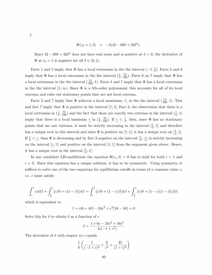
7.

Ψ(c2 = 1, δ) = −4(42− 69δ + 32δ2).

Since 42 − 69δ + 32δ2 does not have real roots and is positive at δ = 0, the derivative of

Φ at c2 = 1 is negative for all δ ∈ (0, 1)

Facts 1 and 5 imply that Φ has a local extremum in the the interval (−1, 15). Facts 5 and 6

imply that Φ has a local extremum in the the interval (15 ,75100). Facts 6 an 7 imply that Φ has

a local extremum in the the interval ( 75100 , 1). Facts 4 and 7 imply that Φ has a local extremum

in the the interval (1,∞). Since Φ is a 5th-order polynomial, this accounts for all of its local

extrema and rules out stationary points that are not local extrema.

Facts 2 and 7 imply that Φ achieves a local maximum, γ, in the the interval ( 75100 , 1). This

and fact 7 imply that Φ is positive in the interval [γ, 1]. Fact 3, the observation that there is a

local extremum in (15 ,75100) and the fact that there are exactly two extrema in the interval (15 , 1)

imply that there is a local minimum γ in (15 ,75100). If γ ≤ 1

2 , then, since Φ has no stationary

points that are not extrema, it must be strictly increasing in the interval [12 , γ] and therefore

has a unique root in this interval and since Φ is positive on [γ, 1], it has a unique root on [12 , 1].

If 12 < γ, then Φ is decreasing and by fact 3 negative on the interval [12 , γ], is strictly increasing

on the interval [γ, γ] and positive on the interval [γ, 1] from the argument given above. Hence,

it has a unique root in the interval [12 , 1].

In any candidate LH-equilibrium the equation Φ(ci, δ) = 0 has to hold for both i = 1 and

i = 2. Since this equation has a unique solution, it has to be symmetric. Using symmetry, it

suffices to solve one of the two equations for equilibrium cutoffs in terms of a common value c,

i.e. c must satisfy

∫ 1

ccβdβ +

∫ c

12

[cβδ + c(1− β)] dβ =

∫ 1

c[cβδ + (1− c)β] dβ +

∫ c

12

[cβδ + (1− c)(1− β)] dβ,

which is equivalent to

1 + c(6 + 4δ)− 24c2 + c3(16− 4δ) = 0

Solve this for δ to obtain δ as a function of c

δ =1 + 6c− 24c2 + 16c3

4c(−1 + c2)

The derivative of δ with respect to c equals

1

8

(1

(−1 + c)2+

2

c2+

45

(1 + c)2

)

40

which is positive. Since δ(1/2) = 0 and the δ-function is strictly increasing for all c < 1, its

invertible. Hence, the candidate solution c(δ) is increasing.

To verify that that the candidate solution c(δ) is indeed an equilibrium for a given value of

δ, it remains to verify that inequality (6) is satisfied by the symmetric cutoff c. As we showed

earlier, this amounts to δ > δ∗ where δ∗ ≈ 0.861276.

A.3 Existence of mixed equilibria

We show existence of equilibria in which there is a common cutoff c and common mixing prob-

ability ξ such that both player use HH for signals above the cutoff and mix for signals below

the cutoff, putting probability ξ on LH and 1 − ξ on HL. Such equilibria exist if and only if

there is an LH equilibrium. The proof proceeds in two steps. First, we show that for any given

mixing probability ξ′ there exists a cutoff c(ξ′) that makes players indifferent at the cutoff be-

tween following the sequences HH and LH. Second, we show that if (and only if) there is an LH

equilibrium, there is a unique mixing probability ξ such that if players use the cutoff c(ξ), they

are indifferent between LH and HL for all signals.

Player 1’s payoff from using the action sequence HH when her signal is α and Player 2 plays

HH for signals β above c, plays LH with probability ξ and HL with probability 1− ξ for signals

below c, equals

HH(α; ξ, c) = 2

∫ 1

cαβdβ + 2

∫ c

12

ξ [α(1− β) + αβδ] + (1− ξ) [αβ + α(1− β)δ] dβ.

If Player 1 uses the action sequence LH instead, her payoff under the same conditions equals

LH(α; ξ, c) = 2

∫ 1

c[(1− α)β + δαβ]dβ

+ 2

∫ c

12

ξ [(1− α)(1− β) + αβδ] + (1− ξ) [(1− α)β + α(1− β)δ] dβ.

In equilibrium these payoffs have to be equal to each other at the equilibrium cutoff. Therefore,

let us look at the (scaled) difference between these payoffs when Player 1’s signal α equals Player

2’s cutoff c:

Ψ(ξ, c) ≡1

2[HH(c; ξ, c)− LH(c; ξ, c)]

= (2c− 1− δc)

∫ 1

cβdβ +

∫ c

12

ξ [(2c− 1)(1− β)] + (1− ξ) [(2c− 1)β] dβ.

It is straightforward to check the following three properties of the function Ψ: Ψ(ξ, 12) =

−δ 12

∫ 112βdβ < 0 ∀ξ ∈ [0, 1]; Ψ(ξ, 1) =

∫ 112ξ(1 − β) + (1 − ξ)βdβ > 0 ∀ξ ∈ [0, 1]; and, Ψ(ξ, c) is

41

continuous in c for all ξ. Therefore, by the intermediate value theorem, for all ξ ∈ [0, 1] there

exists a c(ξ) ∈(12 , 1)such that Ψ(ξ, c(ξ)) = 0.

Note that at any solution c(ξ) of the equation Ψ(ξ, c) = 0, we must have (2c(ξ)−1−δc(ξ)) < 0.

From this fact it follows that ∂Ψ(ξ, c(ξ))/∂c > 0 for all ξ ∈ [0, 1]. This and the fact that Ψ is

continuously differentiable implies that for any ξ ∈ [0, 1] the solution c(ξ) is unique. (To see

this in more detail, suppose first that the set of solutions has an accumulation point c∗(ξ), i.e.

all open neighborhoods of c∗(ξ) contain a solution other than c∗(ξ). By continuity of Ψ, c∗(ξ)

is itself a solution and therefore ∂Ψ(ξ, c∗(ξ))/∂c > 0. This, however, is inconsistent with c∗(ξ)

being an accumulation point of the set of solutions. This implies that for every point there is a

sufficiently small open neighborhood that contains no more than finitely many solutions. This

implies that every compact interval of R contains only finitely many solutions. Now suppose

that there are at least two solutions, c1 and c2 > c1, and consider a compact interval I that

contains c1 and c2. Since there are only finitely many solutions in I, the set of solutions c that

satisfy c > c1 has a smallest element, c. Since ∂Ψ(ξ, c1)/∂c > 0 and ∂Ψ(ξ, c)/∂c > 0, there exist

c′ and c′′ with c1 < c′ < c′′ < c such that Ψ(ξ, c′) > 0 and Ψ(ξ, c′′) < 0. But then continuity of Ψ

and the intermediate value theorem imply that there is a solution in the interval (c1, c), which

contradicts the definition of c.) By the implicit function theorem for any ξ ∈ [0, 1] there exists

an ǫ(ξ) > 0 such that c(ξ) is continuously differentiable for all ξ′ with |ξ′ − ξ| < ǫ(ξ). Since this

is true for all ξ ∈ [0, 1], c(ξ) is continuously differentiable for all ξ ∈ [0, 1].

It remains to show that there is a mixing probability ξ of Player 2 that for all signals α

makes Player 1 indifferent between the action sequences LH and HL when Player 2 uses the

cutoff c(ξ). We first show this for α = 1 and will argue below that this suffices. Player 1’s payoff

from action sequence LH, given signal α = 1 against a Player 2 who mixes with probability ξ

and uses cutoff c(ξ) equals

LH(1; ξ, c(ξ)) =

∫ 1

c(ξ)δβdβ +

∫ c(ξ)

12

ξ [βδ] + (1− ξ) [(1− β)δ] dβ.

Given the same signals and strategy of Player 2, Player 1’s payoff from the sequence HL equals

HL(1; ξ, c(ξ)) =

∫ 1

c(ξ)βdβ +

∫ c(ξ)

12

ξ [(1− β)δ] + (1− ξ) [(βδ] dβ.

Note that both functions are continuous in ξ. Next evaluate both functions at ξ = 0,

LH(1, 0, c(0)) =

∫ 1

c(0)δβdβ +

∫ c(0)

12

[(1− β)δ] dβ,

HL(1; 0, c(0)) =

∫ 1

c(0)βdβ +

∫ c(0)

12

[(βδ] dβ,

42

and observe that LH(1, 0, c(0)) < HL(1, 0, c(0)).

It remains to examine both functions at ξ = 1. Recall that by construction,HH(c(1); 1, c(1)) =

LH(c(1), 1, c(1)). If in addition we have LH(c(1); 1, c(1)) ≥ HL(c(1), 1, c(1)), then c(1) is the

equilibrium cutoff in an LH equilibrium. The condition LH(c(1); 1, c(1)) ≥ HL(c(1), 1, c(1)) is,

however, equivalent to LH(1; 1, c(1)) ≥ HL(1, 1, c(1)) because LH(c(12

); 1, c(1)) = HL(c

(12

), 1, c(1))

and the functions LH(α; 1, c(1)) and HL(α, 1, c(1)) are affine in α. Thus, the intermediate value

theorem implies that such a mixed equilibrium exists whenever there is an LH equilibrium (and

it differs from the LH- equilibrium whenever LH(c(1); 1, c(1)) > HL(c(1), 1, c(1))).

Conversely, if there is no LH equilibrium, then LH(1; 1, c(1)) < HL(1, 1, c(1)). Note that

LH(1; ξ, c(ξ))−HL(1; ξ, c(ξ)) =

∫ 1

c(ξ)(δ − 1)βdβ +

∫ c(ξ)

12

(2ξ − 1)δ(2β − 1)dβ

Since ∂Ψ(ξ, c)/∂ξ =∫ c

12[(2c− 1)(1− 2β)] dβ < 0 and, as we showed above, ∂Ψ(ξ, c(ξ))/∂c > 0,

we have c′(ξ) > 0. Therefore LH(1; ξ, c(ξ)) < HL(1; ξ, c(ξ)) for all ξ ∈ (0, 1), and thus there is

no mixed equilibrium of this type when there is no LH equilibrium.

B Action independence and signal independence

Action independence alone is consistent with perfectly correlated signals about the marginals.

As an examples consider the case of m actions per player and n players who both observe a

common signal that tells them for each of their actions the (marginal) probability that it is part

of a success profile. Unlike in the case we consider in this paper, if the distribution of signals is

atomless, there is an equilibrium that attains ex post efficient exploration with probability one.

Receiving independent signals about the marginals is consistent with violations of action

independence. As an example, consider the case of two players each of whom has three actions

and receives two possible signals, (12 ,12 , 0) or (

13 ,

13 ,

13). The four different combinations of signals

induce for different distributions, indicated as 3× 3-matrices, as follows.

(12

12 0

) (13

13

13

)

12120

12 0 00 1

2 00 0 0

13 0 1

60 1

316

0 0 0

131313

13 0 00 1

3 016

16 0

19

19

19

19

19

19

19

19

19

43

Here, unlike in the case we consider in the paper, if the game has maximally three time periods,

then there exists an ex post efficient equilibrium: First take action 1, then action 2; if both players

received the signal (12 ,12 , 0) the success has been found; otherwise the player who received signal

(12 ,12 , 0) repeats the same two actions and the player who received a signal (13 ,

13 ,

13) takes the

third action.

C Proofs

Proof of Proposition 4

Proof: Suppose not. Then there exists a Player i, a signal ωi and an action history hit

that has positive probability given σ and ωi, following which there is positive probability that

Player i plays an action aij′ that is not maximal. Hence, there exists an action aij′′ with

Prob

(aij′′ , a−i) 6∈ A(ht)∩ (aij′′ , a−i)|a−i ∈ At

−i(σ−i, hit, ωi)| ωi, hit, σ−i > 0 and r(aij′′ , ωi) >

r(aij′ , ωi). Consider the signal ωi for which r(aij , ωi) = r(aij , ωi) ∀j and ωij =1

r(aij′′ ,ωi)for all j

with r(aij , ωi) ≥ r(aij′′ , ωi) and ωij = 0 otherwise. Since σi is an ordinal strategy, it prescribes

the same behavior following (ωi, hit) as it does after (ωi, hit).Now consider the following deviation

after history (ωi, hit) : play a′′ij in period t and then after the resulting history (ωi, (hit, aij′′)) use

the continuation play that the original strategy σi would have prescribed following (ωi, (hit, aij′)).

Now there are two possibilities: Either playing aij′′ does induce a success in period t, or it does

not. In the latter case, there is no loss from the deviation since for the signal ωi there would also

not have been a success from using action aij′ in period t and the sequence of realized action

profiles following period t is identical to the one induced by the original strategy. In the former

case the deviation is profitable because of discounting.

Proof of Proposition 5

Proof: For any strategy profile σ define pt(σ) as the (unconditional) probability of a success in

period t, let Θ+ := t ∈ T |pt(σ) > 0 and Θ0 := t ∈ T |pt(σ) = 0. Recall that for each Player

j, pure strategy sj and signal ωj the action that is induced in period t is denoted by atj(sj , ωj).

We claim that if a profile σ of ordinal strategies is maximal then atj(sj , ωj) = atj(s′j , ωj) ∀t ∈

Θ+, ∀sj , s′j ∈ supp(σj), and for almost all ωj ∈ Ωj . We argue by induction on t. The claim is true

in period 1 because with a maximal strategy Player j will take her highest probability action,

and the probability of a tie among highest probability actions is zero. Suppose t ∈ Θ+ and the

claim holds for all τ < t. With σ−j fixed and the claim being true for all τ < t the maximal

action in period t is independent of which sj ∈ supp(σj) Player j used before time t since by the

inductive hypothesis all of these pure strategies have induce the same action sequences before

44

time t, except possibly in the event of a tie in the probabilities that the signal ωj assigns to

actions, which occurs with probability zero.

Since for all j 6= i we have atj(sj , ωj) = atj(s′j , ωj) ∀t ∈ Θ+, ∀sj , s

′j ∈ supp(σj), for almost

all ωj ∈ Ωj , for periods t ∈ Θ+ Player i’s maximal action, after having adhered to σi before

time t, is the same for all s−i ∈ σ−i. Now consider t ∈ Θ0. Since ordinal strategies are mappings

from histories and rankings into actions, there are only finitely many ordinal pure strategies.

Therefore for every Player j every pure strategy in the support of σj has positive probability.

Therefore if pt(σ) = 0, then pt(σi, s−i) = 0 for all s−i in the support of σ−i. This implies that

any action that is maximal in period t ∈ Θ0 against σ−i remains maximal against every s−i in

the support of σ−i. Together these two observations show that if σi is maximal against σ−i, then

it is also maximal against every s−i in the support of σ−i.

Next, we show that if σi is maximal against the partial profile of pure strategies s−i, then it

is a best reply against that profile. Take any pure strategy si that is in the support of Player

i’s mixed strategy σi. We will show by way of contradiction that si is a best reply against s−i.

Suppose that this is not the case. Then there exists a signal ωi and a pure strategy s′i such

that Player i’s expected payoff conditional on having observed signal ωi satisfies πi(s′i, s−i;ωi) >

πi(s;ωi). Let τ be the first period in which aτ ((s′i, s−i), ω) 6= aτ (s, ω). Note that τ is independent

of ω−i. There are two possibilities: Either aτ ((s′i, s−i), ω) ∈ Aτ−1(s, ω), or aτ ((s′i, s−i), ω) ∈

A \Aτ−1(s, ω) in which case ωi(aτi ((s

′i, s−i), ω)) ≤ ωi(a

τi (s, ω)) since by assumption si assigns a

maximal action after every positive probability history. Let θ > τ be the first period in which

aτ−i(s, ω) = aθ−i(s, ω) in case that such a θ exists. Note that θ is independent of ω.

Consider a strategy s′′i with

ati(s′′i , ω) = ati(s

′i, ω) ∀t 6= τ, θ

aτi (s′′i , ω) = aτi (si, ω)

aθi (s′′i , ω) = aτi (s

′i, ω).

Evidently, either this raises the probability of finding a success in period τ by the same amount

that it lowers it in period θ, or the two probabilities are the same. Because of discounting, in

both cases replacing s′i with s′′i weakly raises the payoff for the signal ωi.

If there is no θ > τ with aτ−i(s, ω) = aθ−i(s, ω), replace s′i with a strategy s′′i such that

ati(s′′i , ω) = ati(s

′i, ω) ∀t 6= τ

aτi (s′′i , ω) = aτi (s, ω).

Evidently, also in this case, the payoff of type ωi weakly increases.

45

Iterating this procedure generates a sequence of action profiles that converges to at(s, ω).

Furthermore the payoff of type ωi is non-decreasing at each step of the iteration, contradicting

the assumption that s′i induces a strictly higher payoff for type ωi than si against s−i. This

confirms that the strategy si is a best response against s−i.

Finally, observe that this is true for every s−i in the support of σ−i and for every si in the

support of σi. It follows that σi is a best reply against σ−i.

Proof of Proposition 7

Proof: If we use (n1, n2, . . . , nI), ni ∈ n ∈ N1|n ≤ mi to label the rank-ordered action profile

in which Player i plays her nith ranked action, the path in which rank-ordered profiles are played

in lexicographic order, (1, . . . 1, 1), (1, . . . , 1, 2) . . ., is maximal. Hence, Proposition 5 implies that

there is always an ordinal equilibrium that induces a search path without repetitions.

From Proposition 4 we know that in any ordinal equilibrium in any period with a positive

success probability each player uses a maximal action. Therefore, every ordinal equilibrium

induces a deterministic sequence of times t at which a novel rank-labeled action profile at is

played; at any other time s players must induce a distribution over rank-labeled action profiles

that have been used earlier and for those times we introduce a generic symbol ∗ that represents

“repetition”. Call any sequence btTt=1 where each bt is either a novel rank-labeled action profile

at or a repetition ∗ an ordinal search path. Clearly, among ordinal search paths, those that induce

repetitions (before all rank-labeled action profiles have been exhausted) are dominated. Since

there are only finitely many ordinal search paths without repetitions, there must be a payoff

maximizing one.

Consider any ordinal equilibrium σ that induces a payoff maximizing search path. Proposi-

tion 4 implies that under σ players choose maximal actions in any period with a positive success

probability by Proposition 4. Hence, the expected payoff from the profile σ is the present dis-

counted value of expected payoffs from profiles of maximal actions. These expected payoffs can

be obtained as follows: Given any signal vector ω, and assuming that Player i takes action aiji

the expected success probability is ω1j1 × ω2j2 × · · · × ωIjI . In case the action taken by play-

ers i corresponds to the nith order statistic of her signal ωi, the expected success probability

equals ω1(n1) × ω2(n2) × · · · × ωI(nI). If each Player i follows the rule ai(ni) the expected success

probability equals ∫

x1 × x2 × · · · × xIdFn1,n2,...nI(x1, x2, . . . , xI)

where Fn1,n2,...nIis the joint distribution of the nith order statistics of all players i. By inde-

pendence, if we let Fnidenote the distribution of the nith order statistic of Player i’s signal ωi,

46

this equals∫

x1dFn1(x1)×

∫

x2dFn2(x2)× · · · ×

∫

xIdFnI(xI)

= ω1(n1) × ω2(n2) × · · · × ωI(nI).

Because of discounting, the strategy profile σ must prescribes to play the rank-labeled action

profiles (a1(n1), a2(n2), . . . , aI(nI)) in the order of the probabilities ω1(n1) × ω2(n2) × · · · × ωI(nI).

Proof of Proposition 8

Proof: We proved that every ordinal equilibrium is an ex post equilibrium in the text.

For the converse consider a pure-strategy ex post equilibrium σ. With pure strategies, if

signals are public, a player knows in every period the set of profiles she can induce in that

period. For example, if it is known that in period t the partial strategy profile σ−i induces the

partial action profile a−i, then Player i can induce the set of profiles P (a−i) := a′ ∈ A|a′−i =

a−i. These sets partition the set of all strategy profiles A. Therefore, whenever a player can

induce the action profile a, the set of profiles she can induce is P (a−i); call this her option

set. With pure strategies and ω public, in any period τ in which her option set, as determined

by profile σ equals O(τ, σ) Player i also knows the subset of profiles N(τ, σ−i, hiτ ) ⊆ O(τ, σ)

that have not already been chosen. Since actions are not observable, Player i’s choice in period

t does not affect her opponents’ choices in periods τ > t. Also, if her option set in period

t is O(t, σ) = P (a−i), then her choice in period t, does not directly affect N(τ, σ−i, hiτ ) in

periods τ > t with O(τ, σ) 6= P (a−i). Therefore, her choice in period t only determines the

probability of a success in that period and the composition N(τ ′, σ−i, hiτ ) in periods τ ′ > t with

O(τ ′, σ) = O(t, σ). Therefore in period t she effectively faces the problem making an optimal

sequence of choices from the set N(t, σ), where each choice induces a fixed probability of a

success. Given discounting, it is optimal to induce profiles in O(t, σ) in decreasing order of the

magnitude of these probabilities, i.e. to take a maximal action in every period. Therefore in an

ex post equilibrium players must use maximal strategies conditional on signals being public. A

pure strategy that is maximal with publicly known signals remains maximal with private signals

because only the ranking of one’s own signal matters in the determination of whether a action

is maximal. Hence, the pure-strategy ex post equilibrium σ is an ordinal equilibrium.

Proof of Proposition 9

Proof: Let the strategy profile σ be an ex post equilibrium profile. In order to derive a con-

tradiction, suppose there is a period and a player who does not play a maximal action in that

47

period. Let τ be the first period in which this is the case and let player i be the player who does

not play a maximal action in period τ. Now consider the case in which each Player j 6= i has

received a signal ωj that puts probability zero on all actions that are ranked lower than their

maximal action in period τ. Then all these players must play their maximal action, denoted a∗j ,

in period τ. This is the case since all other actions in the current period induce a zero success

probability, since a player can always follow the same action sequence in the future as the one

prescribed by σj and since there is no effect on the future play of other players from Player j’s

current choice. Note that each Player k must play her maximal action a∗k in period τ with pos-

itive probability. This is the case because it is strictly optimal to do so for the signal that puts

zero probability on all lower ranked actions, and for any action sequence λ her payoffs are con-

tinuous in her signals. In an ex post equilibrium, i’s maximal action must remain maximal when

all players j 6= i play their maximal action. Suppose not, then a lower ranked action than i’s

maximal action has positive probability of success when all players j 6= i play a∗j but the action

a∗i does not have positive probability of success. Furthermore, this remains true when we restrict

attention to signal realizations for which Player i plays a∗i according to σi. For such signals i

would want to change her behavior ex post. For the signal realization where each Player j 6= i

observes ωj and an action ai that Player i plays with positive probability in period τ according

to σi, the action profile (ai, a−i) has a positive probability of a success in any period t ≥ τ only

if all players j play a∗j . To see this, first note that if any Player j uses a lower ranked action than

her maximal action a∗j , the success probability is zero. Second, observe that since (a∗1, . . . , a∗I)

is maximal in period τ, for any action aiτ that i plays with positive probability in period τ any

action profile (a′1, . . . , a′i−1, ai,τ , a

′i+1, . . . , a

′I) with a′j ≻ a∗j for some j 6= i and a′j a∗j for all j 6= i

has zero probability of inducing a success. This can be shown as follows: Since (a∗1, . . . , a∗I) is

maximal, it follows from before that this action profile is played with positive probability. Hence

(a′1, . . . , a∗i−1, aiτ , a

∗i+1, . . . , a

∗I) has zero probability of inducing a success. Similarly, the profile

(a∗1, a′2, a

∗2, . . . , a

∗i−1, aiτ , a

∗i+1, . . . , a

∗I) has zero probability of inducing a success. Thus both of

these action profiles have been played before and because by assumption in periods prior to τ

only maximal actions have been played, the profile (a′1, a′2, a

∗2, . . . , a

∗i−1, aiτ , a

∗i+1, . . . , a

∗I) must

have have been played before.

Proof of Proposition 10

Proof: Let s be a pure-strategy ordinal equilibrium. For every Player k and any signal ωk that

that player might receive, denote by λk(sk, ωk) the path of Player k’s actions that is induced by

her strategy sk and signal ωk.

48

Note that in an ordinal equilibrium for any Player k and any two signals ωk and ωk with

r(ωk) = r(ωk) we have λk(sk, ωk) = λk(sk, ωk). Since in addition we are only considering pure-

strategy equilibria, it suffices to check that for every Player i, every signal ωi ∈ Ωi of that

player, every partial profile of action sequences λ−i ∈ L(∪ω−i

λ−i(s−i, ω−i))of other players,

and every own action sequence λi(si, ωi), one has

λi(si, ωi) ∈ argmaxλi

u(λ, ω) ∀ ω−i.

This, however, is implied by three facts: (1) fixing any ordinal profile of other players, a

maximal strategy for Player i against that profile is a best response against that profile; (2) a

period is promising for an ordinal strategy profile if and only if it promising for any permutations

of any equilibrium action sequences of other players; and, (3) for Player i the property of a

strategy being maximal is preserved as long as the behavior pattern of other players does not

change, i.e. as long as every other player plays some permutation of one of her equilibrium action

sequences.

Proof of Proposition 11:

We prove this result by showing that it suffices to limit the search for an optimal profile to a

restricted class of strategy profiles, that this class is compact and that the payoff is continuous

in this class. For notational convenience, we use ωi and ωi interchangeably to denote Player i’s

signal in this proof.

As a preliminary step, we first note that the sets of optimal and of Nash equilibrium profiles

can be analyzed in terms of mappings from signals to distributions over action sequences. Since

Player i has mi actions, she can follow one of(mi)T

possible action sequences in the T -period

game. We denote a typical action sequence of this kind for Player i by λi and the set of such

action sequences for Player i by Λi. We show below that in the present environment the sets

of optimal and of Nash equilibrium profiles can be fully characterized in terms of the action-

sequence mappings χi : Ωi → ∆(Λi).

This follows from the following four observations: (1) Any strategy σi induces an action-

sequence mapping χi|σi that assigns the same probability to action sequences as does σi. Con-

versely, (2) for any action-sequence mapping χi we can find a strategy σi for Player i such that

χi = χi|σi. Then (3) if χj |σj = χj |τj for all j 6= i and σi is a best reply to σ−i, then σi is

also a best reply to τ−i; and, (4) any strategy τi with χi|τi = χi|σi is also a best reply to σ−i

and τ−i. Thus for any optimal strategy profile σ there exists an action-sequence mapping χ|σ

that induces the same payoff and conversely for any action sequence mapping χ there exists a

49

strategy profile that induces that mapping. Similarly, for any Nash equilibrium σ the profile of

action-sequences χ|σ retains all relevant information about σ in the sense that any other strategy

profile τ with χ|τ is a Nash equilibrium that induces the same outcome. Conversely, for any

profile χ of action-sequence mappings we can check the best-reply property of Nash equilibrium

directly, without specifying strategies σi beyond the requirement that they induce χi.

For observation (1) note that for any behaviorally mixed strategy σi the action-sequence

mapping χi that is defined by

χi((ai(1), . . . , ai(T ))|ωi) := σi(ai(1)|ωi)×σi(ai(2)|ai(1), ωi)×. . .×σi(ai(T )|ai(1), . . . , ai(T−1), ωi)

for all action sequences (ai(1)), . . . , ai(T )) assigns the same probabilities to action sequences.

For observation (2) note that for given χi any behaviorally mixed strategy that satisfies

σi(ai(t)|ai(1), . . . , ai(t− 1), ωi) =

∑

λi|λi(t′)=ai(t′),t′≤t χi(λi|ωi)∑

λi|λi(t′)=ai(t′),t′≤t−1 χi(λi|ωi)

assigns the same probability to action sequences. Observation (3) follows from the fact that

an action sequence, despite not being a fully specified strategy, does fully determine behavior

after all histories that can be induced by other players. Hence, when Player i deviates her rivals

action-sequence mappings fully determine their response to i’s deviation. Finally, observation

(4) is a simple consequence of the fact that in the present setting any two strategies of Player

i that induce the same action-sequence mappings induce the same outcome and therefore the

same payoff for Player i.

Definition A1 If there exists a finite partition of the signal space of Player i such that her

strategy σi prescribes the same action sequence everywhere on the interior of a given partition

element, σi is a partition strategy.

Definition A2 A convex-partition strategy is a partition strategy based on a partition all of

whose elements are convex.

Since Player i has mi actions, she can follow one of(mi)T

possible action sequences in the

T -period game. Let λit be the action taken by Player i in period t given her action sequence λi.

Each Player i’s strategy can be viewed as a function that maps her signal ωi into a distribution

over action sequences λi. Accordingly, we use σiλi

(ωi)to denote the probability that Player i

plays action sequence λi after observing the signal ωi. ωiλit

denotes the probability that Player

i’s signal ωi assigns to the period-t element of her action sequence λi.

Since we have a common-interest game, we can focus on Player 1 as representative for

all other players. Denote the joint signal distribution of all players other than Player 1 by

50

H(ω2, . . . , ωN

). Then Player 1’s payoff in the T -period game as a function of her chosen action

sequence λ1, her signal ω1 and the strategies of other players σ−1 equals

π(λ1, ω1;σ−1

)=

∫∑

λ2

. . .∑

λN

(σ2λ2

(ω2)× . . .× σN

λN

(ωN))

×

ω1λ11. . . ωN

λN1+ δω1

λ12. . . ωN

λN2

1(λ12,λ

22,...,λ

N2 ) 6=(λ1

1,λ21,...,λ

N1 )

+ . . .

+δTω1λ1T. . . ωT

λNT

1(λ1T,λ2

T,...,λN

T )/∈(λ11,λ

21,...,λ

N1 ),...,(λ1

T−1,λ2T−1,...,λ

NT−1)

dH(ω2, . . . , ωN

)

Inspection of the above payoff function yields the following observation:

Lemma A1 Player i’s payoffs are linear in Player i’s signal ωi, for any given strategies σ−i of

other players and any action sequence λi =(λi1, . . . , λ

iT

)of Player i.

Next we show that Lemma A1 implies that any strategy profile can be replaced by a convex-

partition strategy profile with an at least equally high payoff. Moreover, the latter profile can

be described via a bounded number of points.

Lemma A2 For any strategy profile σ, there exists a profile of convex-partition strategies σ

such that π (σ) ≥ π (σ) and in which each element of Player i’s partition is a convex polytope

with at most M i vertices, where M i ≡((mi)T−1+mi

mi−1

).

Proof: Take σ−i as given. Since Player i’s payoff from a given action sequence λi is linear in

her signal ωi, the set of signals for which a given action profile is optimal satisfies((mi)T − 1

)

linear inequalities that ensure that the payoff from λi is higher than from that from any other

action sequence λi; an additional mi inequalities and one equation ensure that the set of signals

is a subset of the (mi− 1)-dimensional unit simplex. Note that in the mi− 1 dimensional signal

space, a vertex is defined by at least mi − 1 equations. Therefore, in this space an upper bound

on the number of vertices of a polytope that is characterized by k > mi − 1 inequalities is(

kmi−1

). Thus, the set of signals for which a given action profile is optimal must be a convex

polytope with at most((mi)T−1+mi

mi−1

)= M i vertices. Hence, there exists a best response to σ−i

that partitions the signal space of Player i into convex polytopes each of which have at most

M i vertices.

Take any strategy profile σ. Since the set of best responses of Player 1 always includes a

convex-partition strategy in which each element of Player 1’s partition is a convex polytope with

at most M1 vertices, we can replace σ1 by such a convex-partition strategy σ1 without lowering

51

payoffs. We then have a strategy profile given by σ′ = (σ1, σ−i). By the same argument as

above, we can replace Player 2’s strategy with a convex partition strategy σ2 in which each

element of Player 2’s partition is a convex polytope with at most M2 vertices, again without

lowering payoffs. Iterating, we get a convex-partition strategy profile σ such that π (σ) ≥ π (σ)

and in which each element of Player i’s partition is a polytope with at most M i vertices.

Proof: (of Proposition 11) Let π := supσ∈ΣT π(σ) and note that π < 1. Consider a sequence

of strategy profiles σn that satisfies limn→∞ π(σn) = π. By Lemma A2, for each strategy profile

σn in the sequence, we can find a profile of convex-partition strategies σn with π(σn) ≥ π(σn).

Evidently, the sequence σn satisfies limn→∞ π(σn) = π.

Each convex-partition profile σn can be represented as a point in a compact Euclidian space:

Recall that Player i has (mi)T possible action sequences. A convex-partition strategy of Player

i assigns each of those action sequences to the interior of a convex polytope with at most

M i =((mi)T−1+mi

mi−1

)elements. Therefore, a convex-partition strategy of Player i can be viewed

as a point in the set Ξi := ∆(mi−1)×M i×((mi)T−1), where the first mi − 1 components describe

a point in the signal space, the second mi − 1 components describe a point in the signal space

and so on; the first M i such points are the vertices of the convex polytope on which Player i

uses his first action sequence (if the convex polytope assigned to the action sequence has less

than M i vertices, simply repeat one of the vertices; if it has empty interior, the corresponding

action sequence is not used with positive probability), likewise the kth M i-tuple of mi−1-tuples

corresponds to the vertices of the convex polytope on which Player i uses her kth action sequence;

it suffices to specify the convex polytopes associated with ((mi)T − 1) action sequences, because

the convex polytope associated with the remaining action sequence is specified by default.

Hence, there exists a convergent subsequence σnk. Denote the limit of this sequence by σ

and note that σ is a convex-partition strategy profile. For any ǫ ∈ (0, 1) and for each Player

i, we can find a closed subset Φi(ǫ) of the signal space such that all elements of Φi(ǫ) belong

to the interior of elements of the partition induced by σi and the probability that i’s signal

is in Φi(ǫ) satisfies ProbΦi(ǫ) > 1 − ǫ. Since the boundary of each partition element varies

continuously with the vertices defining that element, we also have that for large k everywhere

on Φi(ǫ), the strategy profiles σ and σnkinduce the same action sequence. Hence, the profiles of

action sequences induced by the two strategy profiles differ with as most probability 1− (1− ǫ)I .

Since the maximum payoff difference from any two strategy profiles is bounded, this implies that

the expected payoff from the profile σ must equal π.

52

Proof of Lemma 1

Proof: From Proposition 4 it follows that for any ordinal equilibrium σ, there is a pure-strategy

ordinal equilibrium s that is payoff equivalent to σ. For a given ω, label Player i’ actions in the

sequence in which they are first used by s. Label actions that are not used by s arbitrarily.

Since s is an ordinal equilibrium, ai1 is the action of Player i with the highest probability of

success. In any ordinal equilibrium s, there will be one player, i, who switches in period two, and

another player, k, who does not switch in period two. Modify the behavior of these two players

as follows: Let i never switch from her first-period action when she is certain. Have k switch in

period two to her action ak2 when she is indifferent. Have k otherwise not change her behavior,

except that in case there exists a first period τ > 2 in which aτ (s, ω) = (ak2, a2−k(s, ω)), she

takes the action a2k1, instead of a2k2 in period τ. Formally, define s′ such that s′−i,k = s−i,k,

i.e. s coincides with s′ for all players other than i and k, and

ati(s′i, ω) = ati(si, ω) ∀ωi ∈ Ωi \ E

Ci , ∀t

ati(s′i, ω) = a1i (si, ω) ∀ωi ∈ EC

i , ∀t

atk(s′k, ω) = atk(sk, ω) ∀ωk ∈ Ωk \ E

Ik , ∀t

a2k(s′k, ω) 6= a1k(sk, ω) ∀ωk ∈ EI

k

aτk(s′k, ω) = a1k(sk, ω) ∀ωk ∈ EI

k

atk(s′k, ω) = atk(sk, ω) ∀ωk ∈ EI

k , ∀t 6= 2, τ

There are four possible cases: (1) If Player i is uncertain and Player k is not indifferent, then

the sequence in which cells are examined under the modified strategy profile s′ is the same as in

the original equilibrium s, and therefore payoffs are the same as well. (2) If Player i is certain

and Player k is not indifferent, then Player i is using a dominant action and all other players are

following the same behavior as under s−i. Consequently, the expected payoff cannot be lower

than from all players using strategy s. (3) If Player i is uncertain and Player k is indifferent, the

only effect of changing from s to s′ is that the order in which two cells are visited is reversed.

Furthermore, these cells are only distinguished by Player k’s action and Player k is indifferent.

Hence payoffs are unchanged in this case. (4) If Player i is certain and Player k is indifferent, the

cell examined in period two has a positive success probability under s′, whereas that probability

is zero under s. Furthermore, since Player i is using a dominant action, and all players other

than players i and k do not change their behavior, the overall effect of switching from s to s′

is to move the examination of higher probability profiles forward. Therefore, in this case the

expected payoff increases.

53

Proof of Proposition 12

Proof: Let eij ∈ Ωi be the signal for Player i that assigns probability one to the jth action

of Player i being required for a success profile, and let zi ∈ Ω be the signal that assigns equal

probability to each action of Player i being required for a success profile. Define Ei to be the dis-

tribution of Player i’s signals that assigns probability one to the set of signals ei1, . . . , eiJ(i), zi

and equal probability to all signals in that set.

Let ζn ∈ (0, 1) and ζn → 0. Define Gn,i = ζnEi + (1 − ζn)Fi as the distribution that draws

ωi with probability ζn from the distribution Ei and with probability (1 − ζn) from Fi and let

Gn =∏I

i=1Gn,i. Then Gn,i∞n=1 is a sequence of distributions converging weakly to Fi, denoted

Gn,iw−→ Fi, where each Gn,i has mass points at indifference and at certainty. Let Ei,k be the

distribution of Player i’s signals that assigns probability one to the set of signals Ωi ⊂ Ωi that are

within (Hausdorff) distance 1k from the set ei1, . . . , eimi , zi and that is uniform on Ωi. Define

Hn,i,k = ζnEi,k + (1− ζn)Fi and let Hn,k =∏I

i=1Hn,i,k. Then each Hn,i,k∞k=1 is a sequence of

distribution functions with Hn,i,kw−→ Gn,i where each Hn,i,k has an everywhere positive density,

and Hn,kw−→ Gn.

An optimal ordinal strategy examines a new cell in every period in which that is still feasible.

Since there are only finitely many paths of play that do so, an optimal ordinal strategy σkn for

Hn,k exists. Finiteness of the set of such play paths also implies that there is a subsequence of

Hn,k∞k=1 for which (after reindexing) each σk

n∞k=1 induces the same play path. From now on

consider this subsequence, and pick a strategy σn that induces this path of play.

Given a signal realization ω, denote Player i’s expected payoff from the strategy profile σ by

vi(σ, ω). Then, for any strategy profile σ and signal distribution F, Player i’s expected payoff

Ui(σ, F ) is

Ui(σ, F ) =

∫

vi(σ, ω)dF (ω).

Let 1σ,a,t be the indicator function of the event that profile a is visited for the first time in

period t under strategy σ and let P (a|ω) stand for the probability that the profile a is a success

given the signal vector ω. Then, for an ordinal strategy σ, Player i’s payoff for a fixed ω has the

form

vi(σ, ω) =T∑

t=1

δt−1

(∑

a∈A

1σ,a,t(ω)P (a|ω)

)

.

Here P (a|ω) is a polynomial in the elements of ω and therefore varies continuously with ω.

Since σ is ordinal, for any time t the quantity∑

a∈A 1σ,a,t(ω)P (a|ω) varies continuously with

ω: This holds because variations in ω that do not change the ranking of actions do not affect

the value of the indicator function, and at points ω where the indicator function switches from

54

assigning the value 1 to a′ to assigning it to a′′, we have P (a′|ω) = P (a′′|ω). Taken together,

these observations imply that vi(σ, ω) is continuous in ω. Hence, by weak convergence of Hn,k

to Gn, we have

Ui(σ, Hn,k) → Ui(σ, Gn),

for any ordinal strategy σ. Therefore, σn must be an optimal ordinal strategy for Gn.

For a given Gn, denote by σ′n the improvement strategy for σn, that we constructed in the

proof of Lemma 1. For any given σ′n, σn and ǫ ∈ (0, 14), we define the strategy σǫ

n as follows:

σǫi,n(ωi) =

σi,n(ωi) if |ωi − eij | > ǫ and |ωi − zi| > ǫǫ−xǫ σ′

i,n(zi) +xǫ σi,n(ωi) if |ωi − zi| = x ≤ ǫ

ǫ−xǫ σ′

i,n(eij) +xǫ σi,n(ωi) if |ωi − eij | = x ≤ ǫ

Note that the payoff vi(σǫn, ω) is a continuous function of the signal vector ω. Hence, weak

convergence implies that

Ui(σǫn, Hn,k) → Ui(σ

ǫn, Gn) as k → ∞.

By construction, we have

Ui(σ′n, Gn) > Ui(σn, Gn),

and

Ui(σǫn, Gn) → Ui(σ

′n, Gn) as ǫ → 0.

Since σn is ordinal, the payoff vi(σn, ω) is a continuous function of the signal vector ω. Hence,

weak convergence implies that

Ui(σn, Hn,k) → Ui(σn, Gn) as k → ∞.

Combining these observations, we conclude that for any n, we can find k(n) and ǫ(n) such that

Ui(σǫ(n)n , Hn,k(n)) > Ui(σn, Hn,k(n)).

To conclude, simply let Fn = Hn,k(n).

55

References

Alonso, R., W. Dessein and N. Matouschek [2008], “When Does Coordination Require

Centralization?” American Economic Review 98, 145-179.

Alpern, S. [1976], “Hide and Seek Games,” Seminar, Institut fur hohere Studien, Wien, 26

July.

Alpern, S. [2002], “Rendezvous Search: A Personal Prespective,” Operations Research 50, .

Alpern, A. and S. Gal [2003], The Theory of Search Games and Rendezvous, Dordrecht,

The Netherlands: Kluwer Academic Publishers.

Argote L., S. Beckman and D. Epple [1990]: “The Persistence and Transfer of Learning

in Industrial Settings,” Management Science 36, 140-154.

Austen-Smith, D., and J. S. Banks [1996]: “Information Aggregation, Rationality, and the

Condorcet Jury Theorem,” American Political Science Review 90, 34-45.

Banerjee, A. [1992], “A Simple Model of Herd Behavior,” Quarterly Journal of Economics

107, 797-818.

Becker, Markus C. [2004], “Organizational Routines: A Review of the Literature,” Indus-

trial and Corporate Change 13, 643-677.

Bikchandani, S., D. Hirshleifer and I. Welch [1992], “A Theory of Fads, Fashion,

Custom and Cultural Change as Informational Cascades,” Journal of Political Economy

100, 992-1026.

Blume, A. and A.M. Franco [2007], “Decentralized Learning from Failure,” Journal of

Economic Theory 133, 504-523.

Blume, A., J. Duffy and A.M. Franco [2009], “Decentralized Organizational Learning:

An Experimental Investigation,” American Economic Review 99, 1178-1205.

Blume, A. and P. Heidhues [2006], “Private Monitoring in Auctions,” Journal of Economic

Theory 131, 179211.

Chamley, C.P. [2004], Rational Herds: Economic Models of Social Learning, Cambridge, UK:

Cambridge University Press.

56

Chassang, S. [2010], “Building Routines: Learning, Cooperation, and the Dynamics of In-

complete Relational Contracts,” American Economic Review 100, 448-465.

Chew W.B., T. Bresnahan and K. Clark [1990], “Measurement, Coordination, and Learn-

ing in a Multiplant Network,” in Measures for Manufacturing Excellence, ed. R Kaplan,

129-162, Harvard Business School Press: Boston, MA.

Cohen, M.D. and P. Bacdayan [1994], “Organizational Routines Are Stored As Procedural

Memory: Evidence from a Laboratory Study,” Organization Science 5, 554-568.

Crawford, V. and H. Haller [1990], “Learning how to Cooperate: Optimal Play in Re-

peated Coordination Games,” Econometrica 58, 571-595.

Crawford, V. and J. Sobel [1982], “Strategic Information Transmission,” Econometrica

50, 1431-1451.

Cremer, J., L. Garicano and A. Prat [2007], “Language and the Theory of the Firm,”

Quarterly Journal of Economics 122, 373-407.

Dewatripont, M. and J. Tirole [2005], “Modes of Communication,” Journal of Political

Economy 113, 1217-1238.

Ellison, G. and R. Holden [2010], “A Theory of Rule Development,” MIT working paper.

Eyster, E. and M. Rabin [2005], “Cursed Equilibrium,” Econometrica 73, 1623-1672.

Gibbons, R. [2010], “Inside Organizations: Pricing, Politics, and Path Dependence,” Annual

Review of Economics 2, 337-365.

Gossner, O. and N. Vieille [2003], “Strategic Learning in Games with Symmetric Infor-

mation,” Games and Economic Behavior 42, 25-47.

Grant, R.M. [1996], “Prospering in Dynamically-Competitive Environments: Organizational

Capability as Knowledge Integration,” Organization Science 7, 375-387.

Hayek, F.A. [1945], “The Use of Knowledge in Society,” American Economic Review 35,

519-530.

Jehiel, P. [2005], “Analogy-based Expectation Equilibrium,” Journal of Economic Theory

123, 81-104.

57

Jehiel, P. and F. Koessler [2008], “Revisiting Games of Incomplete Information with

Analogy-based Expectations”Games and Economic Behavior 62, 533-557.

McLennan, A. [1998], “Consequences of of the Condorcet Jury Theorem for Beneficial Infor-

mation Aggregation by Rational Agents,” American Political Science Review 92, 413-418.

March, J. G., and Simon. H. A. [1958], Organizations, John Wiley: New York, NY.

Miller, D. [2011], “Robust Collusion with Private Information,” Review of Economic Studies,

forthcoming.

Nelson, R.R. and S.G. Winter [1982], An Evolutionary Theory of Economic Change,

Belnap Press/Harvard University Press: Cambridge, MA.

Polanyi, M. [1966], The Tacit Dimension, Doubleday & Company, Inc.: Garden City, NY.

Salter W. [1960], Productivity and Technical Change, Cambridge University Press: Cam-

bridge, UK.

Stasser, G. and W. Titus [1985], “Pooling of Unshared Information in Group Decision

Making: Biased Information Sampling During Discussions,” Journal of Personality and

Social Psychology 48, 1467-1478.

Syverson, C. [2011], “What Determines Productivity?,” Journal of Economic Literature 49,

326-365.

United States. Joint Chiefs of Staff. Special Operations Review Group. [1980]

Rescue Mission Report. Washington, DC. Available at:

http://www.history.navy.mil/library/online/hollowayrpt.htm#execsum

Wiseman, T. [2005], “A Partial Folk Theorem for Games with Unknown Payoff Distributions,”

Econometrica 73, 629-645.

58