© Copyright by Zoha Nasizadeh, 2014

Validation of a New and Cost Effective Technique to

Estimate Reservoir Pressure and Permeability in

Low-Permeability Reservoirs

A Thesis

Presented to

the Faculty of the Department of Petroleum Engineering

University of Houston

In Partial Fulfillment

of the Requirements for the Degree

Master of Science

in Petroleum Engineering

by

ZOHA NASIZADEH

December 2014


Estimate Reservoir Pressure and Permeability in

Low-Permeability Reservoirs

Zoha Nasizadeh

Approved:

Chair of the Committee Dr. W. John Lee, Hugh Roy and Lillie Cranz Cullen Distinguished University Chair Professor Petroleum Engineering

Committee Members: John Adams, Unconventional Resource COP Leader and Advisor BP America Inc.

Dr. Arthur Weglein, Hugh Roy and Lillie-Cranz Cullen Distinguished Professor Dept. of Physics Dept. of Geosciences, Reflection Seismology

Dr. Suresh Khator, Associate Dean Cullen College of Engineering

Dr. Thomas K. Holley, Professor and Director Petroleum Engineering

v

Acknowledgements

I would like to express my special appreciation and thanks to my advisor,

Dr. John Lee, for his invaluable advices and guidance throughout this project. He

was always supportive, encouraging and willing to share his ever more

fascinating ideas which were crucial to the success of this work.

I would like to thank John Adams and Bryan Dotson for their guidance and

support through my research. They provided several field data which were critical

part of this research. I am especially grateful to my committee members, Dr.

Arthur Weglein, and John Adams for their sound advices and inputs towards the

completion of this work.

I would like to thank Dr. Thomas Holly, Ms. Anne Sturm, and all

professors in Petroleum Engineering Department at the University of Houston for

providing opportunities and resources to complete this research work.

A special thanks to my family and friends. Words cannot express how

grateful I am to my mother and father, Parvin and Ehsan for all of the sacrifices

they have made for me. Similarly, I am grateful to my parents in law for their

emotional encouragements. I am thankful to my lovely sister and brothers who

motivated me through all stages of my education. I would also like to thank all of

my friends for their good company and their assistance during this work.

Last but not least, I would like to express my deepest appreciation to my

beloved husband, Rohollah who have supported me in every possible way. My

achievements would have not been possible without his help and inspiration. To

whom I dedicate this thesis.

vi


Estimate Reservoir Pressure and Permeability in Low-

Permeability Reservoirs

An Abstract

of a

Thesis

Presented to

the Faculty of the Department of Petroleum Engineering

University of Houston

In Partial Fulfillment

of the Requirements for the Degree

Master of Science

in Petroleum Engineering

by

ZOHA NASIZADEH

December 2014

vii

Abstract

I developed the mathematical basis for a new and cost effective method to

estimate reservoir pressure and effective water permeability in low permeability

reservoirs. This method, called Baseline/Calibration, was successfully tested in

Wamsutter fields. This approach, which is an alternative to time-consuming DFIT

tests and conventional pressure buildup tests, requires injection of water in

multiple short stages. Sandface pressure and flow rate are analyzed to estimate

reservoir pressure and permeability.

I derived analytical expressions which provide a mathematical basis for

this method. The analytical formulations are based on transient solutions to the

diffusivity equation, the principle of superposition, and assume piston-like

displacement of reservoir fluids with injected water.

I constructed several numerical simulation models and validated the

proposed technique. I also analyzed flow rate and pressure data from two field

trials performed in the Almond formation of the Wamsutter field. The results of

numerical simulation and field trials of this method verified that our method

accurately determines reservoir pressure with short injection tests.

Reservoir pressure is a fundamental property of the reservoir and its

depletion provides an insight in to the reservoir dynamics and drainage pattern.

Measurements of formation pressure and in-situ reservoir permeability are

important for a variety of reasons including estimation of ultimate recovery,

production forecasting, and optimization of depletion planning.

viii

Unconventional gas reservoirs are economically viable hydrocarbon

prospects that have proven to be very successful. However, conventional well

tests methods are often impractical in unconventional reservoirs. Long shut-in

times are required for estimates of reservoir pressure and reservoir permeability.

ix

Table of Contents

Acknowledgements ........................................................................................................... v

Abstract ............................................................................................................................ vii

Table of Contents ............................................................................................................. ix

List of Figures .................................................................................................................. xii

List of Tables ................................................................................................................ xviii

Nomenclature ................................................................................................................. xix

1.1 Problem Statement .................................................................................... 1

1.2 Literature Review ...................................................................................... 2

1.2.1 Diagnostic Fracture Injection Test in Unconventional Reservoirs . 2

1.2.2 After-Closure Analysis .................................................................... 5

1.2.3 Pseudo-Radial Flow Regime ........................................................... 6

1.2.4 Bi-Linear Flow Regime ................................................................... 7

1.2.5 Linear Flow Regime ........................................................................ 8

1.3 Research Objective .................................................................................... 9

1.4 Review of Chapters ................................................................................. 10

2.1 Introduction ............................................................................................. 12

x

2.2 Baseline/Calibration Technique .............................................................. 12

2.3 Mathematical Principle ........................................................................... 13

2.3.1 Solution to Diffusivity Equation ................................................... 14

2.3.2 Principle of Superposition in Time ............................................... 20

2.3.3 Piston-Like Displacement of Gas by Water .................................. 24

2.3.4 Superposition of Steady-State and Transient Pressures ................ 25

2.4 B/C Analysis - Pressure Calculation ....................................................... 26

2.5 B/C Analysis- Permeability Calculation ................................................. 28

3.1 Introduction ............................................................................................. 31

3.2 Reservoir description ............................................................................... 31

3.2.1 Petrophysical Properties ................................................................ 33

3.2.2 Fluid Properties ............................................................................. 34

3.2.3 Rock-Fluid Properties ................................................................... 36

3.2.4 Initial Conditions ........................................................................... 36

3.3 Description of Validation Case Studies .................................................. 36

4.1 Introduction ............................................................................................. 39

4.2 Mathematical Solution for a Single-Phase Water ................................... 39

4.3 Mathematical Solution for Two-Phase Flow Gas and Water .................. 42

xi

4.4 Baseline/Calibration Case Studies .......................................................... 44

4.4.1 Formation with 0.01 mD Permeability .......................................... 45

4.4.2 Formation with 0.1 mD Permeability ............................................ 51

4.4.3 Formation with 0.001 mD Permeability ........................................ 58

5.1 Introduction ............................................................................................. 66

5.2 Field Trial One ........................................................................................ 67

5.3 Field Trial Two ........................................................................................ 71

References ........................................................................................................................ 78

xii

List of Figures

Figure 1-1: Typical diagnostic fracture injection test, injection rate and pressure

response (Cramer and Nguyen, 2013). ............................................................ 3

Figure 2-1: Constant flow rate injection during a baseline/calibration test. .................... 20

Figure 2-2: Baseline/calibration trend alignment. ............................................................ 29

Figure 2-3: Baseline/Calibration supercharging correction. The alignment pressures

are plotted versus the corresponding cumulative injected water. A linear

trend line passes through these points and extrapolated back to the zero

cumulative injection. The final estimate of reservoir pressure is 5250

psi. .................................................................................................................. 30

Figure 3-1: 2D grid top view of numerical reservoir model in I and J directions. .......... 32

Figure 3-2: 2D grid top view of numerical reservoir model in I and K directions. ......... 32

Figure 3-3: Three dimensional grid top view of numerical reservoir model. .................. 33

Figure 3-4: Gas formation volume factor and viscosity are functions of pressure in

all reservoir simulation models. ..................................................................... 35

Figure 3-5: Assumed gas compressibility factor is a function of pressure in all

reservoir simulation models. .......................................................................... 35

Figure 3-6: Relative permeability curves for the reservoir rock studied in this thesis.

Variables and are relative permeability of gas and water,

respectively. ................................................................................................... 36

Figure 3-7: Time variation of injection rate for B/C test when performed for a

formation with permeability equal to 0.01 mD. ............................................ 38

xiii

Figure 4-1: Schedule of constant injection rates in different stages for a numerical

simulation model with single phase water. .................................................... 40

Figure 4-2: Comparison of calculated bottom-hole pressure with that obtained using

CMG-IMEX for a simulation case study of single-phase water flow. ......... 41

Figure 4-3: Comparison of bottom-hole pressure calculated with the function

and that obtained from CMG-IMEX for a simulation case study of

single-phase water flow. In contrast to Figure 4-2, in this figure,

function is used instead of the logarithmic approximation to calculate

bottom-hole pressure. .................................................................................... 42

Figure 4-4: Comparison of calculated bottom-hole pressure with that obtained using

simulator CMG-IMEX in a case study with two phases of gas and water.

Formation permeability is assumed to be 0.01 mD. ...................................... 44

Figure 4-5: Numerical simulation output for a case study with two phases of gas

and water. Formation permeability is assumed to be 0.01mD. This

figure shows cumulative injected water and bottom-hole pressure (BHP)

versus time. .................................................................................................... 45

Figure 4-6: Baseline/calibration alignment for a numerical simulation model with

permeability equal to 0.01 mD. (a) First B/C pair is aligned at 5258 psi,

(b) second B/C pair is aligned at 5274 psi, and (c) third B/C pair is

aligned at 5282.2 psi. ..................................................................................... 47

xiv

Figure 4-7: Baseline/calibration supercharging correction for a case study with

permeability equal to 0.01 mD. The linear trend line passes through

pressure match points and extrapolated to zero cumulative water

injected. 2 for the linear trend line is 0.96. The final estimate of initial

reservoir pressure is 5251.7 psi. .................................................................... 48

Figure 4-8: Average pressure of invaded area versus cumulative injection water. At

onset of injection period between each pair, average pressures agree

well with alignment B/C pressures. ............................................................... 49

Figure 4-9: Average pressures of invaded zone versus time. Pressure alignment

points are approximately the same as average pressures at the end of

each shut-in time. ........................................................................................... 50

Figure 4-10: Radial profile of water saturation at the end of injection and shut-in

times. In this case study, formation permeability is equal to 0.01 mD. ......... 51

Figure 4-11 : Time variation of water injection rate for a B/C test when performed

for a formation with a permeability equal to 0.1 mD. ................................... 52

Figure 4-12: Numerical simulation output for a case study with gas and water

phases. Formation permeability is assumed to be 0.1mD. This figure

shows cumulative injected water and bottom-hole pressure (BHP)

versus time. .................................................................................................... 52

Figure 4-13: Baseline/calibration alignment for a reservoir with 0.1 mD

permeability. (a) First B/C pair is aligned at 5251 psi, (b) second B/C

pair is aligned at 5252 psi, and (c) third B/C pair is aligned at 5253 psi. ...... 53

xv

Figure 4-14: Baseline/calibration supercharging correction for reservoir simulation

with permeability 0.1 mD. A linear trend line was drawn through


injected. 2 for the linear trend line is 0.97. The final estimate of

reservoir pressure is 5250.9 psi. .................................................................... 55

Figure 4-15: Average pressures of invaded zone versus cumulative injected water

for a numerical simulation with permeability equal to 0.1 mD.

Alignment Pressures have good agreement with average reservoir

pressures at the end of shut-in times. ............................................................. 56

Figure 4-16: Average pressures versus time for a numerical simulation with

permeability 0.1 mD. Alignment pressures are approximately the same

as average pressure of invaded zone at the end of shut-in times. .................. 57


times. In this case study, formation permeability is equal to 0.1 mD. ........... 57

Figure 4-18 : Time variation of injection rate for B/C test when performed for a

formation with permeability equal to 0.001 mD. .......................................... 58

Figure 4-19: Numerical simulation output for a reservoir with two phases of gas

and water. Formation permeability is assumed to be 0.001mD. This

figure shows cumulative water injected and bottom-hole pressure (BHP)

versus time. .................................................................................................... 60

Figure 4-20: Baseline/calibration alignment for a case study with 0.001 mD

permeability. (a) First B/C pair is aligned at 5271 psi, (b) second B/C

pair is aligned at 5311 psi, and (c) third B/C pair is aligned at 5347 psi. ...... 61

xvi

Figure 4-21: Baseline/calibration supercharging correction for reservoir simulation

with permeability 0.001 mD. The linear trend line passes through


injected. 2 of the linear trend line is 0.98. The final estimate of

reservoir pressure is 5259.9psi. ..................................................................... 62

Figure 4-22: Average pressures of invaded zone versus cumulative water injected

for a numerical simulation with permeability 0.001 mD. The alignment

pressures are approximately the same as average pressures at the end of

shut-in times. .................................................................................................. 63

Figure 4-23: Average pressures of invaded area versus time for a numerical

simulation with permeability 0.001 mD. Alignment pressures are

approximately the same as average pressures at the end of shut-in times. .... 64


times. In this case study, formation permeability is equal to 0.001 mD. ....... 65

Figure 5-1: Time variation of injection rate during baseline/calibration field trial

one. This test was conducted with FFLT protocol. ....................................... 68

Figure 5-2: Cumulated injected water and sandface pressure during

baseline/calibration field trial one. ................................................................ 69

Figure 5-3: Baseline/calibration trend alignment for the field trial one. (a) First pair

is aligned at 4850 , (b) second pair is aligned at 5050 , and (c)

third pair is aligned at 5200 . ................................................................... 70

xvii

Figure 5-4: Supercharging correction for baseline/calibration field trial one. A

linear trend line passes through pressure points and extrapolates to zero

cumulative water injected. 2for this linear trend line is 0.97. .................... 71

Figure 5-5: Time variation of injection rate during baseline/calibration field trial

two. This test was conducted with FFLT protocol. ....................................... 72

Figure 5-6: Cumulated injected water and sandface pressure during

baseline/calibration field trial two. ................................................................ 72

Figure 5-7: Baseline/calibration trend alignment for the field trial two. (a) First pair

is aligned at 4900 , (b) second pair is aligned at 5325 , and (c)

third pair is aligned at 5600 . ................................................................... 74

Figure 5-8: Supercharge correction for baseline/calibration field trial two. A linear

trend line passes through pressure points and extrapolates to zero

cumulative water injected. 2for this linear trend line is 0.87. .................... 75

xviii

List of Tables

Table 3-1: Assumed properties of the water component .................................................. 34

Table 3-2: Initial conditions assumed for numerical reservoir model. ............................ 37

Table 4-1: Summary of cumulative injected water, reservoir pressure match, and

average slope for each pair of baseline/calibration trends. In this

simulation, formation permeability is assumed to be 0.01 mD. .................... 46



simulation, formation permeability is assumed to 0.1 mD. ........................... 54



simulation, formation permeability is assumed to 0.001 mD. ....................... 61

Table 5-1: Summary of cumulative injected water and alignment reservoir pressure

for each baseline/calibration trend, field trial one. ........................................ 69

Table 5-2: Summary of cumulative injected water and alignment reservoir pressure

for each baseline/calibration trend, field trial two. ........................................ 73

xix

Nomenclature

Variables

= Reservoir area, ft

= Formation volume factor of water, RB/STB

= Formation compressibility, 1/psi

= Gas compressibility, 1/psi

= Oil compressibility, 1/psi

= Total reservoir compressibility, 1/psi

= Water compressibility, 1/psi

= Exponential integral function, dimensionless

= Reservoir height, ft

= Formation Permeability, mD

= Effective gas permeability, mD

= Effective water permeability, mD

= Fracture Conductivity, mD-ft

= Fracture half length, ft

= Reservoir pressure, psi

= Average pressure of invaded zone, psi

= Reference pressure, psi

= Dimensionless pressure, dimensionless

= Bottom-hole pressure, psi

= Initial reservoir pressure, psi

xx

= Real gas pseudo-pressure, psi /cp

= Transient pressure gradient, psi

= Steady state pressure gradient, psi

= Flow rate, STB/d

= Cumulative injected water, bbl

= Radius of investigation, ft

= Dimensionless radius, dimensionless

= Radius of invasion, ft

= Wellbore radius, ft

= Residual gas saturation, dimensionless

= Initial water saturation, dimensionless

= Dimensionless time, dimensionless

= Time at ith injection or shut-in time, hour

= injection time, hour

= Temperature, °R

= Volumetric flow rate in radial direction, RB/Dft2

= Injected volume, bbl

= shut-in time, hour

= Gas mobility, mD/cp

= Total mobility, mD/cp

= Water mobility, mD/cp

= Viscosity, cp

xxi

= Viscosity of gas phase, cp

= Viscosity of oil phase, cp

= Viscosity of water phase, cp

= Fluid density, lbm/ft

= Density at p , lbm/ft

= Reservoir porosity, dimensionless

1

Introduction

Unconventional gas reservoirs are economically viable hydrocarbon

prospect that have proven to be very successful in the United States. More than

fifty percent of the currently identified gas resources in the United States are

unconventional (Adams et al., 2012). This research is guided towards exploring

methods to estimate formation pressure in unconventional reservoirs.

In this chapter, I describe the problem and motivation for developing a

new method for estimation of formation pressure and permeability in

unconventional reservoirs. I present a review of literature for existing methods

and mathematical formulations to estimate formation pressure and permeability,

a list of objectives, and a brief review of all chapters included in this thesis.

1.1 Problem Statement

Pressure is a fundamental property of a reservoir and its depletion

provides an insight into the reservoir dynamics and drainage pattern.

Understanding the reservoir depletion behavior is necessary in optimizing field

development. Estimation of reservoir properties such as formation pressure, in-

situ reservoir permeability, and closure pressure is important for variety of

reasons including estimation of ultimate recovery, production forecasting, and

optimization of depletion planning (Adams et al., 2012). Furthermore, completion

2

designs, modeling studies, and future field development decisions are all

improved with better knowledge of current and historical reservoir pressures

(Adams et al., 2013).

Performing conventional transient tests is practically challenging in

unconventional gas reservoirs because the formation permeability is very low in

unconventional gas reservoirs. Even though well-known conventional well testing

methods are applicable in unconventional reservoirs, however, they are often

impractical because of long shut-in time (Jin et al., 2013). There is lack of a

practical method to estimate formation pressure and permeability in a cost

effective way.

1.2 Literature Review

Several methods are currently in use to obtain formation pressure and

permeability in tight gas reservoirs. The most popular method to estimate

formation properties in unconventional reservoirs is Diagnostic Fracture Injection

Test (DFIT). In this section, I briefly review the main structure of DFIT, different

types of analysis, and advantages and disadvantages of this method.

1.2.1 Diagnostic Fracture Injection Test in Unconventional Reservoirs

The diagnostic fracture injection test (DFIT) or minifrac test is an

invaluable tool to evaluate reservoir properties and geomechanical

characteristics in unconventional formations. The diagnostic fracture injection test

is used to estimate reservoir pore pressure, permeability, and state of stress in

the rock strata (Cramer and Nguyen, 2013). This method is conducted before the

3

main fracturing treatment. DFIT is a process in which the fracturing fluid is

injected at a constant rate and high pressure to propagate a small fracture into

the formation. After achieving the formation fracture pressure, surface injection is

stopped to evaluate and analyze the declining pressure response. Figure 1-1

represents a typical diagnostic fracture injection test (Cramer and Nguyen, 2013).

Figure 1-1: Typical diagnostic fracture injection test, injection rate and pressure

response (Cramer and Nguyen, 2013).

The following steps are taken during a typical diagnostic fracture injection

test (Cramer and Nguyen, 2013):

1) A surface pump is installed to inject water or any other fracturing fluid in to

the wellbore and the wellbore fluid is pressurized. The compression time is

a function of injection rate, wellbore volume, and formation breakdown

pressure.

2) A hydraulic fracture propagates into the reservoir when breakdown

pressure is reached.

4

3) Water injection continues until wellhead pressure becomes stable. This

step causes the fracturing fluid to leak off into the formation.

4) Surface injection is stopped and consequently pressure declines rapidly.

At this time, an instantaneous shut-in pressure (ISIP) is observed.

5) The shut-in well pressure is recorded and analyzed for signs of fracture

closure. Fracture closure pressure is considered to be the same as

minimum principal stress.

6) The declining pressure response is evaluated during “after closure period”

to observe the signatures of pseudo-linear and pseudo-radial flow

regimes.

Before planning a DFIT, it is necessary to define the test objectives.

Defining the objectives will help to determine when the test should end and what

kind of analysis should be performed (Martin et al., 2013). If the objective is to

measure fracture closure pressure, the test can be stopped at the onset of the

fracture closure signature from the declining pressure data. Fracture closure

pressure could be estimated using “before-closure analysis”. If the objective is to

evaluate formation transmissibility ( / and pore pressure ( , then DFIT ends

at the onset of the observation of signatures corresponding to pseudo-radial, bi-

linear, and linear flow regimes. “After-closure” period is evaluated during pseudo-

radial, bi-linear, and linear flow regimes. Transmissibility and pore pressure can

be derived using pseudo-radial flow solution method, and pore pressure can be

obtained from linear flow solution method. In this section, I explain “after-closure

analysis” in which we can estimate initial formation pressure and transmissibility.

5

1.2.2 After-Closure Analysis

After-closure analysis is based on a conventional well test technique

called short-term formulation. However, it has been shown that this technique is

valid for after-closure data of a diagnostic fracture injection test (Soliman et al.,

2005). The majority of conventional well test methods and diagnostic test

method are characterized by very short injection or production time followed by a

relatively long shut-in time. In the short-term test technique, the principle of

superposition is not used to drive the solution for a buildup test. Instead, the

coupled flow rate and drawdown/buildup test are solved directly (Soliman, 1986).

If a DIFT is considered as an injection/shut-in test with similarity to the

regular injection falloff test, the short-term formulation could be used to analyze

the declining pressure data (Soliman et al., 2005). A DFIT is not the same as

injection falloff test due to induced fracture during pumping period. At the

presence of induced fracture short-term test technique should not be used for

“after closure analysis”. However, due to shortness of injection time, the short-

term test formulation may be applicable to the declining DFIT pressure with high

degree of accuracy (Soliman and Kabir, 2012).

The flow regime reached after sufficient amount of shut-in time depends

on the properties of reservoir, fluid, and fracture closure. Here, I present how the

method of short-term formulation can be applied to find initial reservoir pressure

and transmissibility from different flow regimes including pseudo-radial, linear,

and bi-linear flow regimes.

6

1.2.3 Pseudo-Radial Flow Regime

The pseudo-radial flow regime is reached when the far field area affected

by flow is circular. Reaching this flow regime requires the propagated fracture to

be fairly short, formation permeability to be relatively high, and formation

compressibility to be low. In other words, it is expected to observe pseudo-radial

flow regime more in liquid reservoirs than in tighter gas reservoirs (Soliman et al.,

2005).

The behavior of the declining pressure data during pseudo-radial flow

regime is shown in Equation (1-1). The presence of pseudo-radial flow regime

indicates that either the fracture is very short or it is completely closed with little

or no residual conductivity. Equations (1-2) and (1-3) are the specialized log-log

and derivative forms of Equation (1-1), respectively, and are expressed as

1694.4 1

Δ, (1-1)

log log1694.4

log Δ , and (1-2)

log log1694.4

log Δ . (1-3)

In Equations (1-1) through (1-3), and are respectively, the reservoir pressure

and initial reservoir pressure in psi. is the injected volume in , is viscosity

in , is reservoir permeability in , is reservoir depth in , is injection

time in hour, and Δ is shut-in time in hour.

Equation (1-2) indicates that if a pseudo-radial flow regime dominates the

reservoir behavior, a plot of left hand-side versus total time Δ on a log-log

7

graph yields a straight line with a slope of -1. Equation (1-3) can be used to

diagnose a pseudo-radial flow regime because it is independent of initial

reservoir pressure. Therefore, plotting the left-hand side of Equation (1-3) vs. the

total time on a log-log graph would result a straight line with a slope equal to -1.

Therefore, plotting Equation (1-3) could be used to identify different flow regime.

After determining the pseudo-radial flow regime, pressure and time data are

plotted according to Equation (1-1) to obtain initial reservoir pressure. Equations

(1-1) through (1-3) are used to estimate transmissibility, however, it is

recommended to use Equation (1-2) for this purpose (Soliman et al., 2005).

1.2.4 Bi-Linear Flow Regime

The bi-linear flow regime can be observed when the propagated fracture is

long or is open with some residual conductivity. The bi-linear flow regime

indicates that the pressure drop in the reservoir is controlled by two linear flow

systems: (i) a linear flow inside the fracture and (ii) a linear flow inside reservoir

and at the vicinity of fracture.

Equation (1-4) describes the behavior of pressure data when bi-linear flow

regime is observed. Equations (1-5) and (1-6) are the log-log and derivative

forms of Equation (1-4), respectively (Soliman et al., 2005), and are expressed

as

264.6 . 1 . 1 1

Δ

.

, (1-4)

8

log log 264.6 . 1 . 1

0.75 log Δ , and (1-5)

log log 198.45 .1 . 1

0.75 log Δ . (1-6)

In the above equations, is reservoir porosity, is total reservoir compressibility

in 1/ , and is fracture conductivity in mD-ft. Equation (1-6) can be used

for diagnostic plot because it is only a function of observed pressure, total time,

and the flow regime. This plot yields a straight line with slope of -0.75 for a bi-

linear flow regime. The initial reservoir pressure can be determined using

Equation (1-4).

1.2.5 Linear Flow Regime

If the induced fracture is fairly long, and it stays open for a long time with high

residual conductivity, a linear flow regime will be observed. Reaching a linear

flow regime during a DFIT is rare, but it might happen if the formation

permeability is low and the DFIT is conducted using an injection fluid containing

proppant (Soliman et al., 2005).

Equation (1-7) describes the behavior of a reservoir pressure when a

linear flow regime signature is observed. Equations (1-8) and (1-9) are log-log

and derivative forms of Equation (1-7), respectively (Soliman et al., 2005), and

are given by

31.054

.1

Δ

.

, (1-7)

9

log log 31.054

.

. 5 log , and (1-8)

log log 15.5254

.

. 5 log , (1-9)

where is fracture half length in .

A diagnostic plot using Equation (1-9) is independent of initial reservoir

pressure, and can be used to determine a linear flow regime. This plot will yield a

straight line with a slope of -0.5. Equation (1-7) can be applied to determine initial

reservoir pressure.

There are several benefits for conducting a diagnostic fracture injection

test. Formation geomechanical properties, minimum in-situ stress, and fracture

closure pressure can be estimated using “before closure analysis” (Soliman et

al., 2013). Moreover, initial reservoir pressure and transmissibility can be

determined using “after closure analysis”. However, reaching to a bi-linear or a

pseudo-radial flow regime, to find and , can be very time consuming and

costly; it often requires multiple days of shut-in. These long shut-in times are not

practical in some cases where it delays the fracture stimulation operations

(Adams et al., 2013).

1.3 Research Objective

The main objective of this research is to develop the mathematical basis

of a cost effective technique to determine initial reservoir pressure and

permeability in unconventional formations by:

10

developing an analytical solution for pressure variations during

injection/shut-ins,

validating the developed equation and baseline/calibration method in

different types of tight gas sand formation,

correcting the estimated pressure from supercharging effect, and

investigating a practical method to calculate formation permeability.

1.4 Review of Chapters

I conducted the following steps to achieve the objectives of this research:

Constructed several synthetic reservoir simulation case studies to perform

sequential steps of baseline/calibration method. The synthetic cases

included different petrophysical rock types which are representative of the

tight gas sand of Wamsutter field.

Performed baseline/calibration method to estimate formation pressure and

compare with the assumed initial pressure values. This step validated

numerically the baseline/calibration method in tight gas sand formations.

Applied currently developed techniques in pressure transient analysis to

estimate pressure and investigated a procedure to calibrate each

technique to better estimate formation permeability.

Applied baseline/calibration technique to estimate formation pressure

using field test data.

In Chapter 2, I describe the baseline/calibration algorithm as well as the

mathematical formulations used in this method. I discuss assumptions, solution

11

to the diffusivity equation with a line source, the principles of superposition in

time, and piston-like displacement of water.

Chapter 3 describes the numerical simulation model, properties of

assumed reservoir, properties of reservoir fluid, and relative permeability curves.

I present several case studies to validate the developed baseline/calibration

method.

I analyze the results of numerical simulations for estimating reservoir

pressure and permeability using baseline/calibration method in Chapter 4.

Chapter 5 discusses the results of baseline/calibration method on real

field data. Chapter 6 summarizes the conclusions of the thesis.

12

Baseline/Calibration Method

2.1 Introduction

The baseline/calibration (B/C) method is a new and cost effective

technique to estimate reservoir pressure in unconventional gas reservoirs.

Measuring reservoir pressure and formation permeability in low permeability gas

reservoirs are difficult with current available practices (Adams et al., 2013).

However, performing a B/C test and the subsequent analysis will enable us to

estimate formation pressure and permeability in a shorter time and for less cost

than other current techniques. In this chapter, I describe the procedure for

baseline/calibration technique, subsequent analysis of the test data, and the

mathematical formulations for the validity of this algorithm with appropriate

assumption.

2.2 Baseline/Calibration Technique

The baseline/calibration method consists of two main parts. The first part

consists of injection of water in discrete stages using different number of

protocols. The second part is the analysis of the pressure and flow rate recorded

from the first part. In the following sections, I show a scheme for plotting pressure

and rate data which enables measuring formation pressure (Adams et al., 2013).

Later, I developed a method to estimate reservoir permeability using the slope of

13

plotted curves. The B/C method should be conducted after perforation and before

the main stimulation job.

A baseline/Calibration test consists of a series of injection events in

different stages. I use sandface pressure and injection rate to generate one or

more pairs of trend lines, called baseline and calibration trends. Different test

protocols can be used to obtain pressure and rate data. These protocols are

constant pressure injection test (CPIT), constant rate injection test (CRIT), and

falling fluid level test (FFLT). CPIT consists of injection at a constant bottom-hole

pressure followed by a short shut-in time. In this protocol, injection rate is

changing during injection stage. CRIT consists of injection at a constant rate

while bottom-hole pressure is changing. FFLT consists of injection by changing

sandface rate and pressure at the same time.

In this study, I used constant rate injection test protocol to perform my

numerical simulations and to derive the analytical solution. Once sandface rate

and pressure data are obtained, I plotted calibrated baseline trends based on the

mathematical formulations described in the following section.

2.3 Mathematical Principle

Mathematical principle for baseline/calibration method is based on the

solution to the diffusivity equation, the principle of superposition in time, and

piston-like displacement of reservoir fluid with injected water. I describe each of

these concepts in the following sections.

14

2.3.1 Solution to Diffusivity Equation

The partial differential equation corresponding to the transient pressure

response of a single phase flow in a reservoir is obtained by a combination of

three physical principles:

1. the principle of mass conservation,

2. Darcy’s law , and

3. an equation of state for reservoir fluid.

The mass conservation equation, which is known as continuity equation, is

given by,

1 , (2-1)

where r is the radius of investigation, is fluid density, is the volumetric flow

rate, is reservoir porosity, is time. Dacy’s law is expressed as

, (2-2)

where is permeability and is fluid viscosity. The equation of state for a slightly

compressible fluid is

, (2-3)

where is the density at the reference pressure and is fluid compressibility.

The radial diffusivity equation of a single phase can be obtained by

combining Equations (2-1) through (2-3), and is given by (Lee et al., 2003)

1,

(2-4)

where is total formation compressibility and is defined as

15

. (2-5)

In the above equation, c is formation compressibility. Equation (2-4) is based on

the following assumptions,

radial flow,

laminar flow,

porous medium has constant compressibility and permeability,

negligible gravity effects,

isothermal conditions,

fluid has small and constant compressibility, and

compressibility times pressure gradient squared product, , is

negligible.

The diffusivity equation for fluid flow in a reservoir is a partial differential

equation of pressure with respect to both space and time. To solve this equation,

an initial condition and two boundary conditions are required.

Initial Condition

It is assumed that the reservoir is initially at a constant and uniform

pressure throughout the reservoir given by

, 0 . (2-6)

Outer-Boundary Condition

An infinite-acting reservoir flow is defined as a reservoir in which the

influence of reservoir boundaries is not felt during the time in which pressure and

16

rate data are analyzed. This is the case when a well is producing at early times

and the effect of outer boundaries of reservoir are not seen; i.e., the reservoir

acts as if there were no boundaries (Matthews and Russell, 1967).

For an infinite acting reservoir, at infinite distance from the wellbore, the

reservoir pressure remains as initial pressure, , for all times (Lee et al., 2003).

Equation (2-7) expresses the outer-boundary condition as,

→ ∞, . (2-7)

Inner-Boundary Condition

If a well produces at a constant sandface rate, flow rate at the wellbore,

, can be described with Darcy’s law. Equation (2-8) expresses the inner-

boundary condition in oil field unit (Lee et al., 2003) as,

141.2. (2-8)

To solve the diffusivity equation, it is convenient to use dimensionless variables.

In oil field units, the dimensionless pressure, time and radius are defined as

,

141.2, (2-9)

0.0002637, and (2-10)

. (2-11)

Substituting Equations (2-9) through (2-11) into Equation (2-4) yields

dimensionless diffusivity equation as

17

1. (2-12)

Dimensionless initial and boundary conditions are shown in Equations

(2-13) through (2-15),

, 0 0, (2-13)

lim→

1, and (2-14)

lim→

, 0. (2-15)

Equation (2-12) is solved using Laplace transformation (Lee et al., 2003). The

line source solution in the form of dimensionless variables is given by

, 1

2

4, (2-16)

where is the exponential integral. The exponential integral is defined as

.

(2-17)

Substituting dimensionless parameters in Equation (2-16), offers the

pressure as a function of time and radius as

,70.6

948

. (2-18)

Lee et al. (2003) show the line-source solution in Equation (2-18) is accurate if

time is

3.975 10 948. (2-19)

18

When the argument of the function, , is less than 0.01, Equation

(2-18) can be further simplified using an approximation for the function. This

approximation for 0.01 is

ln 1.781 . (2-20)

Therefore, substituting the above equation into Equation (2-18) gives pressure as

70.6 ln

1688. (2-21)

Bottom-hole pressure is calculated by substituting into Equation (2-21),

and is given by

70.6

ln1688

. (2-22)

Equation (2-22) is the transient flow solution for single phase radial flow.

The transient flow equation for a reservoir containing gas can be obtained in a

similar way and it is given by (Economides et al., 2013)

1638 log 3.23 , (2-23)

where is reservoir temperature in ° and is the gas flow rate in / .

is the real gas pseudo-pressure function and is defined as

2 , (2-24)

where is arbitrary reference pressure.

The diffusivity equation for a reservoir with multi-phase flow is similar to

the diffusivity equation for single phase flow (Martin, 1959). The only difference is

19

the use of total mobility, , and a total compressibility . The diffusivity equation

for radial flow of a multi-phase system is given by

1.

(2-25)

The total mobility of a three phase system is defined as

, (2-26)

and the total compressibility is given by

. (2-27)

The similarity between the single phase and multi-phase flow equations implies

that the solution to diffusivity equation of a single phase flow also applies to the

multi-phase flow.

I used a water-gas flow system in my numerical simulations. The transient

flow equation for multi-phase flow of a gas-water system is

70.6

ln1688

, (2-28)

where

(2-29)

and

. (2-30)

The solution to the multi-phase flow diffusivity equation assumes that the

saturation gradients in drainage area of the well are small.

20

2.3.2 Principle of Superposition in Time

The principle of superposition in time is used to solve the variable rate

production problem. Figure 2-1 shows the time variation of flow rate during a B/C

test. In a baseline/calibration test, the well goes through a series of water

injection and shut-in schedules. The constant flow rate varies in discrete injection

stages. Peters (2012) used the principle of superposition to find the solution of

reservoir pressure during variable injection rate. I used this technique to find

pressure as function of time during B/C test.

Figure 2-1: Constant flow rate injection during a baseline/calibration test.

According to the principle of superposition in time, when , the

dimensionless pressure solution is given by

Flow Rate

Time

q1

q2

q3

q4

t1 t2 t3 t4 t5 t6 t7

21

, , 0 ,

0 , 0 ,

0 , 0 ,

0 , 0 , , (2-31)

where

, 1

2

4and (2-32)

, 1

2

4.

(2-33)

The other dimensionless pressures are calculated from equations similar to

Equation (2-33). Dimensionless flow rate is defined as

,

(2-34)

where is the reference flow rate which is usually assumed to be the flow rate

in the first stage, i.e., (Lee et al., 2003).

At the wellbore 1, hence, the dimensionless bottom-hole pressure is

calculated by

,

. (2-35)

By substituting the dimensionless parameters and using the approximation of

function, Equation (2-35) becomes

22

141.2

1

2ln

1688ln

1688

ln1688

ln1688

ln1688

ln1688

ln1688

ln1688

. (2-36)

Equation (2-36) applies to a reservoir with single phase liquid flow. The pressure

solution for two phase flow is similar to single phase flow. The only difference is

the use of total mobility and total compressibility. Therefore, for a reservoir

containing gas and water, pressure response is

141.2

1

2ln

1688ln

1688

ln1688

ln1688

ln1688

ln1688

ln1688

ln1688

, (2-37)

where

(2-38)

and

. (2-39)

23

In order to calculate average reservoir pressure, I define ∗ as the time at

the onset of injection. Average reservoir pressure is expressed in Equation

(2-40),

∗ and (2-40)

∗ . (2-41)

On the other hand, I showed that is a function of time, i.e.,

and (2-42)

. (2-43)

By substituting Equation (2-43) in Equation (2-41), I obtain

∗ . (2-44)

Average pressure, , defined by Equation (2-40) is expressed as

70.6

ln1688

∗. (2-45)

Therefore, f t∗ corresponding to Equation (2-40) is given by

f t∗70.6q B

λ h

q

qln

1688 ϕc r

λ t t∗. (2-46)

Similarly, I used Equation (2-37) to find f t :

70.6 ln

1688ln

1688

ln1688

ln1688

ln1688

ln1688

ln1688

ln1688

.

(2-47)

Substituting and ∗ into Equation (2-44), yields

24

70.6

ln1688

ln1688

ln1688

ln1688

ln1688

ln1688

ln1688

ln1688

ln1688

∗.

(2-48)

2.3.3 Piston-Like Displacement of Gas by Water

During a baseline/calibration test procedure, water is injected into the

reservoir which creates a piston-like displacement profile within a distance from

the wellbore. This distance is called the radius of invasion . The radius of

invasion is a function of time and cumulative water injected. Assuming piston-like

displacement of gas by water, radius of invasion can be calculated using a

volumetric equation (Satter et al., 2008), namely,

5.615 1 , (2-49)

where is total water injected in , is initial water saturation (unitless), and

is residual gas saturation (unitless). is the area in , and is given by

. (2-50)

By substituting Equation (2-50) in Equation (2-49), I can found as a

function of cumulative injected water, porosity, thickness, wellbore radius, initial

water saturation, and residual gas saturation, namely,

25

5.615

1, (2-51)

Because water is much more viscous than gas, it is plausible to assume a piston-

like water displacement profile during water injection. In the radius of invasion,

the pressure response is governed by a steady-state pressure gradient, that is,

Δ 141.2

ln , (2-52)

where is the injection rate in / (Peters, 2012).

2.3.4 Superposition of Steady-State and Transient Pressures

Using results from previous sections, I superposed the pressure gradient

across the piston-like profile of water and through water to outer reservoir

boundary to obtain the pressure response at the wellbore during a B/C test. In

other words, the pressure at the wellbore is a combination of the steady-state

pressure gradient (Equation (2-52)) and the transient pressure response

(Equation (2-37)), namely,

Δ . (2-53)

In the above equation

141.2

2ln

1688ln

1688

ln1688

ln1688

ln1688

ln1688

ln1688

ln1688

, (2-54)

26

for ,and is calculated using Equation (2-52).

2.4 B/C Analysis - Pressure Calculation

In this work, I discuss only the mathematical formulations for the B/C test

performed under injection with constant flow rate. Sandface flow rate and

pressure pairs are recorded during a baseline/calibration test. The analysis of

these data consists of a plot of versus Δ / . Δ / is given by

Δ, (2-55)

and is calculated using Equation (2-51). According to Equation

(2-54), when , is

141.2

2ln

1688. (2-56)

If I assume , then can be calculated as

141.2

2ln

141.2ln . (2-57)

Therefore is calculated using

Δ

141.2

ln 141.2

ln

(2-58)

27

141.2

1 1

ln .

By rearranging the above equation, I obtain

141.21 1

ln . (2-59)

Similarly, for other time intervals, Δ / can be expressed similar to

Equation (2-59). According to Equation (2-59), a plot of ln versusΔ /

should be linear for a correct assumption of initial reservoir pressure. In the B/C

technique, a plot of the first injection stage generates a baseline trend and the

plot for the second injection stage generates a calibration trend (see Figure 2-2).

These trend lines align linearly if the assumed reservoir pressure is correct. If the

assumed reservoir pressure is too high, then the two trend lines do not align and

the calibration trend shifts to the right of baseline trend. On the other hand, if the

assumed reservoir pressure is too low, then the calibration trend shifts to the left

of baseline trend (Adams et al., 2013). Therefore, in an iterative manner,

reservoir pressure can be estimated by calibrating the baseline.

Additional injection stages provide more baseline and calibration trends.

For instance, the second injection stage can be a baseline trend where the third

injection stage is the calibration trend, and this sequence continues. Each pair of

baseline and calibration trends is aligned at a value which is an estimate of

reservoir pressure. Each pair yields a separate estimated initial reservoir

pressure; the collection of these pairs provides multiple values as reservoir

28

pressure. Each injection stage disturbs the formation, hence, the B/C technique

find different initial pressure (Abdollah-Pour, 2011). Therefore, a correction

method is designed to correct the baseline/calibration supercharging near the

wellbore which is caused by injection.

Figure 2-2 demonstrates the trend alignment for a B/C test with three

injection stages. This is the results of a numerical simulation where assumed

reservoir pressure is 5250 psi. The B/C analysis shows the first pair of

baseline/calibration trends are in alignment at 5290 , and the second

pair of baseline/calibration trends are aligned at 5345 . Note that the

estimated reservoir pressure increases from 5290 psi to 5320 psi from the first

pair to the second pair. This effect is called B/C supercharging (Adams et al.,

2013). To correct the B/C supercharging, matching pressure points are plotted

versus the corresponding cumulative injection water. A linear trend line passes

through these points and extrapolated back to the zero cumulative injection as

shown in Figure 2-3. The final estimate of reservoir pressure is the pressure at

the zero cumulative water injection where reservoir has not been disturbed yet.

2.5 B/C Analysis- Permeability Calculation

Using baseline/calibration analysis, I develop a method to estimate

effective permeability to water phase in the reservoir. According to Equation

(2-59), a plot of ln versus should be linear with a constant slope. This

constant slope is given by

29

141.21 1

. (2-60)

Since ≫ , the term 1/ can be neglected. Thus slope is approximated

as

141.2. (2-61)

(a) 5100 , calibration trends are shifted to left meaning the assumed is too low.

(b) 5290 , best trend alignment for stages 1 and 2.

(c) 5345 , best trend alignment for stages 2 and 3.

(d) 5800 ,calibration trends are shifted to right meaning the assumed is too high.

Figure 2-2: Baseline/calibration trend alignment.

0

0.1

0.2

0.3

0.4

0.5

0.6

0.7

0 200 400 600

ln(re/rw)

dp/q (psi/Gpd)

Stage 1

Stage 2

Stage 3

0

0.1

0.2

0.3

0.4

0.5

0.6

0.7

0 100 200 300 400

ln(re/rw)

dp/q (psi/Gpd)

Stage 1

Stage 2

Stage 3

0

0.1

0.2

0.3

0.4

0.5

0.6

0.7

‐200 0 200 400

ln(re/rw)

dp/q (psi/Gpd)

Stage 1

Stage 2

Stage 3

0

0.1

0.2

0.3

0.4

0.5

0.6

0.7

‐400 ‐200 0 200 400

ln(re/rw)

dp/q (psi/Gpd)

Stage 1

Stage 2

Stage 3

30

I used the slope of the alignment of the last pair to find the effective

permeability of water. Using known values of fluid viscosity, thickness, and water

formation volume factor, effective permeability of water is calculated as

141.2. (2-62)

Figure 2-3: Baseline/Calibration supercharging correction. The alignment pressures are plotted versus the corresponding cumulative injected water. A linear trend line passes through these points and extrapolated back to the zero cumulative injection. The final estimate of reservoir pressure is 5250 psi.

31

Numerical Model Simulation

3.1 Introduction

In this chapter, I present several baseline/calibration test models

constructed using a numerical simulation software to validate the results from this

technique. I compared the results of baseline/calibration technique from simulator

with those obtained from mathematical formulations I developed. I performed

assessment of the validity of this method in formations with different

permeabilities and defined the applicability range for baseline/calibration method.

I used a commercial reservoir simulator from Computer Modeling Group

Ltd. (CMG). The variations of composition, phase behavior, and temperature are

negligible in these tests. Hence, a conventional black oil simulator, CMG-IMEX

was used to accurately model the case studies.

3.2 Reservoir description

In this study, a one dimensional (1D) radial reservoir model with a radius

of 300 feet was constructed with 300x1x1 grids. A wellbore with 0.341 feet radius

is located in the middle of the reservoir. Grid blocks are designed logarithmically

to have smaller grids toward the wellbore and larger grids farther from the

wellbore. Figure 3-1 and Figure 3-2 show two-dimensional (2D) top and side

views of a numerical reservoir model in i-j and i-k directions, respectively. A

32

three dimensional (3D) grid top view of numerical simulation model is presented

in Figure 3-3.

Figure 3-1: 2D grid top view of numerical reservoir model in I and J directions.

Figure 3-2: 2D grid top view of numerical reservoir model in I and K directions.

33

Figure 3-3: Three dimensional grid top view of numerical reservoir model.

3.2.1 Petrophysical Properties

The reservoir simulation model is assumed to have a porosity of 8 percent

and initial water saturation of 20 percent. Previous experimental studies have

shown that residual gas saturation under water drive can be extremely high,

between 15 to 50 percent of pore volume (Geffen et al., 1952). A value of 35% of

pore volume is often used in field practices when specific information about

residual gas saturation is not available (Agarwal et al., 1965). Recently, Merletti

et al. (2013) performed petrophysical evaluations of Wamsutter tight gas sand

formations and found a range of 20 to 45 percent for residual gas saturation. In

34

this study, I chose value of 35 percent for residual gas saturation in all reservoir

simulation models.

In this study, rock compressibility is assumed to be 2 10 1/ at

reference pressure of 5250 . For simplicity, the reservoir model thickness is

assumed to be 1 ft. I set up three different numerical case studies, with formation

permeability values of 0.001, 0.01, and 0.1 mD. I assess the validity of B/C

technique on all case studies. In all of these reservoir models, / is assumed

to be 0.1.

3.2.2 Fluid Properties

The numerical reservoir models with which the baseline/calibration

technique was tested consisted of two phases; water and gas. Table 3-1

describes properties of the water phase.

Table 3-1: Assumed properties of the water component

Parameter Unit Value

Water compressibility 1/psi 3.159 x 10-6

Viscosity cp 0.472

Density lb/ft 61.638

Figure 3-4 shows assumed viscosity and formation volume factor for the

gas phase in this study. Gas compressibility factor is a function of pressure and

is shown in Figure 3-5.

35

Figure 3-4: Gas formation volume factor and viscosity are functions of pressure in all reservoir simulation models.

Figure 3-5: Assumed gas compressibility factor is a function of pressure in all reservoir simulation models.

‐0.05

0

0.05

0.1

0.15

0.2

0.25

0

0.01

0.02

0.03

0.04

0.05

0.06

0 2000 4000 6000 8000 10000 12000

Form

ation Volume Factor (RB/Scf)

Viscosity (cp)

Pressure (Psi)

Viscosity

Bg

0

0.2

0.4

0.6

0.8

1

1.2

1.4

1.6

0 2000 4000 6000 8000 10000 12000

Gas Compressibility Factor

Pressure (psi)

36

3.2.3 Rock-Fluid Properties

I assume the formation rock is water wet and initial water saturation is 20

percent whereas residual gas saturation is 35 percent. Figure 3-6 shows the

assumed relative permeability curves for the reservoir rock model.

Figure 3-6: Relative permeability curves for the reservoir rock studied in this thesis. Variables and are relative permeability of gas and water, respectively.

3.2.4 Initial Conditions

Initial conditions for numerical reservoir model are described in Table 3-2.

I assumed the depth of water-gas contact is 10,100 ft and at the reservoir depth,

water is at the irreducible level.

3.3 Description of Validation Case Studies

For validation purposes and finding the range of formation permeability

where baseline/calibration method is applicable, I created three different

0

0.1

0.2

0.3

0.4

0.5

0.6

0.7

0.8

0.9

1

0 0.2 0.4 0.6 0.8 1 1.2

Relative Perm

eab

ility

Sw

Krw

Krg

37

reservoir simulation models, with permeabilities of 0.001, 0.01, 0.1 mD. In a

recent study, Almond reservoir sands exhibited porosities in the range of 6 to 16

percent and absolute permeabilities ranging from 0.003 to 3 mD (Merletti et al.,

2013). Merletti et al. (2013) showed that a single porosity value can exhibit

permeabilities varying by 3 orders of magnitude (i.e. a rock with porosity value of

10 percent, have permeability ranges between 0.001mD to 1mD). I chose the

same porosity of 8 percent for all of reservoir simulation rock types with different

permeabilities.

Table 3-2: Initial conditions assumed for numerical reservoir model.

Parameter Unit Value

Reservoir Temperature °F 150

Initial Reservoir Pressure psi 5250

Reservoir Top Depth ft 10000

I used a constant rate injection method to simulate the B/C test. For

example for a reservoir with the permeability of 0.01 md, I modeled 4 different

injection stages with constant rates of 0.05, 0.07, 0.09, and 0.11 bbl/day with 4

shut-in times between each set of two injection stages. Each injection stage and

shut-in time lasted 36 minutes. Figure 3-7 represents time variation of injection

rate for B/C test when performed for a formation with permeability equal to 0.01

md.

38

Figure 3-7: Time variation of injection rate for B/C test when performed for a formation with permeability equal to 0.01 mD.

0

0.02

0.04

0.06

0.08

0.1

0.12

0.14

0 50 100 150 200 250 300

Injection Rate (bbl/d)

Time (min)

39

Results

4.1 Introduction

In this chapter, I present the validation of the mathematical formulations

which were described in Section 2.3. For this purpose, I compared results

obtained using mathematical formulations with those obtained from reservoir

simulation models.

Initially, I studied the mathematical formulation corresponding to a

reservoir containing single-phase water. Afterwards, I tested the mathematical

formulations for a reservoir with two phases of water and gas. I present the

results of the baseline/calibration test and analysis for different numerical

simulation models.

4.2 Mathematical Solution for a Single-Phase Water

In simulation of a reservoir containing single phase water, I used the initial

conditions summarized in Table 3-2. I assumed reservoir permeability is 0.01mD

and the depth of water-gas contact is 9000 ft. Therefore, there is only a single

phase water at the depth of assumed reservoir, 10,000 ft. In a B/C test

procedure, the fluid injected was water; therefore, a single phase fluid flowed in

this test case.

In this simulation, I assumed water injection in 4 stages. Figure 4-1

shows the injection schedule.

40

Figure 4-1: Schedule of constant injection rates in different stages for a numerical simulation model with single phase water.

The bottom-hole pressure is calculated using Equation (2-36). Figure 4-2

compares the bottom-hole pressure obtained from simulator (solid black line)

with those calculated using bottom-hole pressure of Equation (2-36), (dashed red

line). Equation (2-36) was described as

141.2

1

2ln

1688ln

1688

ln1688

ln1688

ln1688

ln1688

ln1688

ln1688

.

(2-36)

0

0.02

0.04

0.06

0.08

0.1

0.12

0.14

0 100 200 300 400 500 600

Water Injection Rate(bbl/d)

Time(min)

41

In Figure 4-2, calculated bottom-hole pressures do not exactly match

bottom-hole pressures obtained from simulator for a very short time (Δ 10

day) at the onset of each injection stage. This is due to the fact that is very

small at the beginning of each stage, and the approximation of the function is

not accurate (see section Solution to Diffusivity Equation). If I use the

function instead of natural logarithm approximation in Equation (2-36), the

calculated is identical to bottom-hole pressure results from simulator.

Figure 4-3 compares calculated using the function to obtained from

the simulator CMG-IMEX.

Figure 4-2: Comparison of calculated bottom-hole pressure with that obtained using CMG-IMEX for a simulation case study of single-phase water flow.

0 0.05 0.1 0.15 0.2 0.25 0.3 0.35 0.40

5000

10000

15000

Time (Day)

Pw

f (p

si)

Calculated Pwf

Pwf from CMG-IMEX

42

Figure 4-3: Comparison of bottom-hole pressure calculated with the function and that obtained from CMG-IMEX for a simulation case study of single-phase water flow. In contrast to Figure 4-2, in this figure, function is used instead of the logarithmic approximation to calculate bottom-hole pressure.

4.3 Mathematical Solution for Two-Phase Flow Gas and Water

For the simulation of a reservoir containing two phases, gas and water, I

assumed the initial condition described in Table 3-2. I assumed formation

permeability is 0.01 mD, reservoir depth is 10,000 ft, and the depth of water-gas

contact is 10,100 ft. Therefore, at the reservoir depth, water saturation is at the

irreducible level (20 percent in these simulations). I assumed petrophysical, fluid,

and rock-fluid properties as described in Chapter 3.

0 0.05 0.1 0.15 0.2 0.25 0.3 0.35 0.40

5000

10000

15000

Time (Day)

Pw

f (p

si)

Calculated Pwf

Pwf from CMG-IMEX

43

I assumed injection of water in 4 discrete stages similar to that described

in Figure 3-7. Each injection and shut-in stage lasted 36 minutes. The bottom-

hole pressure for a two-phase flow is governed by Equation (2-53) as

Δ , (2-53)

where

141.2

2ln

1688ln

1688

… ln1688

ln1688

… ln1688

ln1688

… ln1688

ln1688

(2-54)

and

Δ 141.2

ln . (2-52)

Figure 4-4 compares the calculated bottom-hole pressures using

Equation (2-53) with that obtained with numerical simulation. It is observed that

bottom-hole pressure calculated using Equation (2-53) has a very good

agreement with that obtained from numerical simulator.

44

Figure 4-4: Comparison of calculated bottom-hole pressure with that obtained using simulator CMG-IMEX in a case study with two phases of gas and water. Formation permeability is assumed to be 0.01 mD.

4.4 Baseline/Calibration Case Studies

In this section, I present the validation of the baseline/calibration method

using numerical case studies for formations with permeability values of 0.001,

0.01, and 0.1 mD. In all these simulations, both gas and water phases were

flowing. Reservoir and fluid properties are those described in Chapter 3.

0 0.05 0.1 0.15 0.25000

5500

6000

6500

7000

7500

Time (Day)

Pw

f (p

si)

Calculated Pwf

Pwf from CMG-IMEX

45

4.4.1 Formation with 0.01 mD Permeability

For the simulation of this case study of B/C test, I considered injection of

water in 4 different stages as shown in Figure 3-7. Figure 4-5 exhibits bottom-

hole pressure and cumulative water injected during testing time from the

simulator.

Figure 4-5: Numerical simulation output for a case study with two phases of gas and water. Formation permeability is assumed to be 0.01mD. This figure shows cumulative injected water and bottom-hole pressure (BHP) versus time.

Baseline/calibration analysis consists of a graph of

versus . Initial pressure, ,is estimated through an iterative method by

aligning each pair of baseline and calibration trends. Figure 4-6 presents the

0 0.05 0.1 0.15 0.20

0.2

0.4

Q (

ga

l)

Time (day)

0 0.05 0.1 0.15 0.24000

6000

8000

BH

P (

ps

i)

Cum Water Injected

BHP

46

best alignment for first, second, and third pairs of baseline and calibration trends.

Each injection stage disturbed the formation, hence, the B/C technique finds

different pressures. Table 4-1 shows that each pair of baseline and calibration

trends is aligned at a different pressure. This is called the B/C supercharging

effect and it needs to be corrected. Therefore, a correction method is designed to

correct the baseline/calibration supercharging near the wellbore caused by

injection.

Table 4-1 summarizes reservoir pressure from calibrated baseline

method and their corresponding cumulative injected water. Moreover, the

average slope of baseline and calibration trends for each pair (used to calculate

permeability) are listed in Table 4-1.


average slope for each pair of baseline/calibration trends. In this simulation, formation permeability is assumed to be 0.01 mD.

Pair Q (gal) Pr-match (psi) Slope (Gpd/psi)

1 0.052 5258 0.0015

2 0.125 5274 0.0016

3 0.218 5284.2 0.0015

47

Figure 4-6: Baseline/calibration alignment for a numerical simulation model with permeability equal to 0.01 mD. (a) First B/C pair is aligned at 5258 psi, (b) second B/C pair is aligned at 5274 psi, and (c) third B/C pair is aligned at 5282.2 psi.

The baseline/calibration supercharging was corrected in the following way:

(i) calibrated baseline reservoir pressures were plotted versus their cumulative

injected water; (ii) a linear trend line was drawn through matching pressure

points, and extrapolated to zero cumulative water injection; (iii) final estimated

reservoir pressure is the pressure at zero cumulative injected water where

reservoir was at initial condition. Figure 4-7 shows B/C pressure and correction

0 100 200 300 400 5000

0.2

0.4

0.6

0.8

Ln

(re/

rw)

dp/q (psi/gpd)(a) First B/C Pairs Aligned

0 100 200 300 400 5000

0.2

0.4

0.6

0.8

Ln

(re/

rw)

dp/q (psi/gpd)(b) Second B/C Pairs Aligned

-100 0 100 200 300 4000

0.2

0.4

0.6

0.8

Ln

(re

/rw

)

dp/q (psi/gpd)(c) Third B/C Pairs Aligned

Stage 1Stage 2Stage 3Stage 4

48

of supercharging effect. Final estimate of reservoir pressure is 5251.7 psi with

0.032% error. The error was calculated by

%, ,

,100. (4-1)

Figure 4-7: Baseline/calibration supercharging correction for a case study with permeability equal to 0.01 mD. The linear trend line passes through pressure match points and extrapolated to zero cumulative water injected. for the linear trend line is 0.96. The final estimate of initial reservoir pressure is 5251.7 psi.

In Figure 4-8, I compared the alignment matching pressure with average

pressure within the invaded area. It turns out that alignment pressures are

approximately the same as average pressures at the end of each shut-in time.

Figure 4-8 displays calculated average pressures versus cumulative injected

water. Pressures at alignments are shown in blue point. Figure 4-9 shows the

0 0.1 0.2 0.3 0.45250

5260

5270

5280

5290

5300

Q (gal)

Pre

s (p

si)

Pr_final 5251.7

Error% 0.031599

Pr_final 5251.7

Error% 0.032

49

agreement between average pressure along the radius of invasion and alignment

B/C pressures as a function of time.

Figure 4-8: Average pressure of invaded area versus cumulative injection water. At onset of injection period between each pair, average pressures agree well with alignment B/C pressures.

Next, using Equation (2-62), I calculated effective water permeability equal

to 0.0024 mD. The maximum value of effective water permeability for this

simulation model was

0.01 0.3 0.003 , (4-2)

when 1 .

0 0.05 0.1 0.15 0.2 0.25 0.3 0.355250

5300

5350

5400

CumW

(Gal)

Pa

vg (

ps

i)

Avg Pr

Alignment Pressure

50

During the simulated B/C test, as shown in Figure 4-10, water saturation does

not reach to the maximum level, 1 . Therefore, the calculated of 0.0024

mD is less than 0.003 and represents the average effective water permeability in

the radius of invasion. Using the rock-fluid properties, described in Figure 3-6, I

estimated gas effective permeability as .

.∗ 0.0024 0.0064 .

Figure 4-9: Average pressures of invaded zone versus time. Pressure alignment points

are approximately the same as average pressures at the end of each shut-in time.

0 0.05 0.1 0.15 0.25250

5300

5350

5400

Time (Day)

Pa

vg (p

si)

Avg Pr

Alignment Pressure

51

Figure 4-10: Radial profile of water saturation at the end of injection and shut-in times. In this case study, formation permeability is equal to 0.01 mD.



using a numerical reservoir model with a formation permeability of 0.1 mD.

Reservoir and fluid properties are those described in Chapter 3. For the

simulation of this case study of the B/C test, I considered injection of water in 4

different stages as shown in Figure 4-11. Figure 4-12 shows time variation of

bottom-hole pressures and cumulative injected water values.

0.4 0.5 0.6 0.7 0.8 0.9 10.1

0.2

0.3

0.4

0.5

0.6

0.7

0.8

Radial Distance (ft)

Wa

ter

Sa

tura

tio

n

Time = 36 min

Time = 72 min

Time = 108 min

Time = 144 min

Time = 180 min

Time = 216 min

Time = 252 min

Time = 288 min

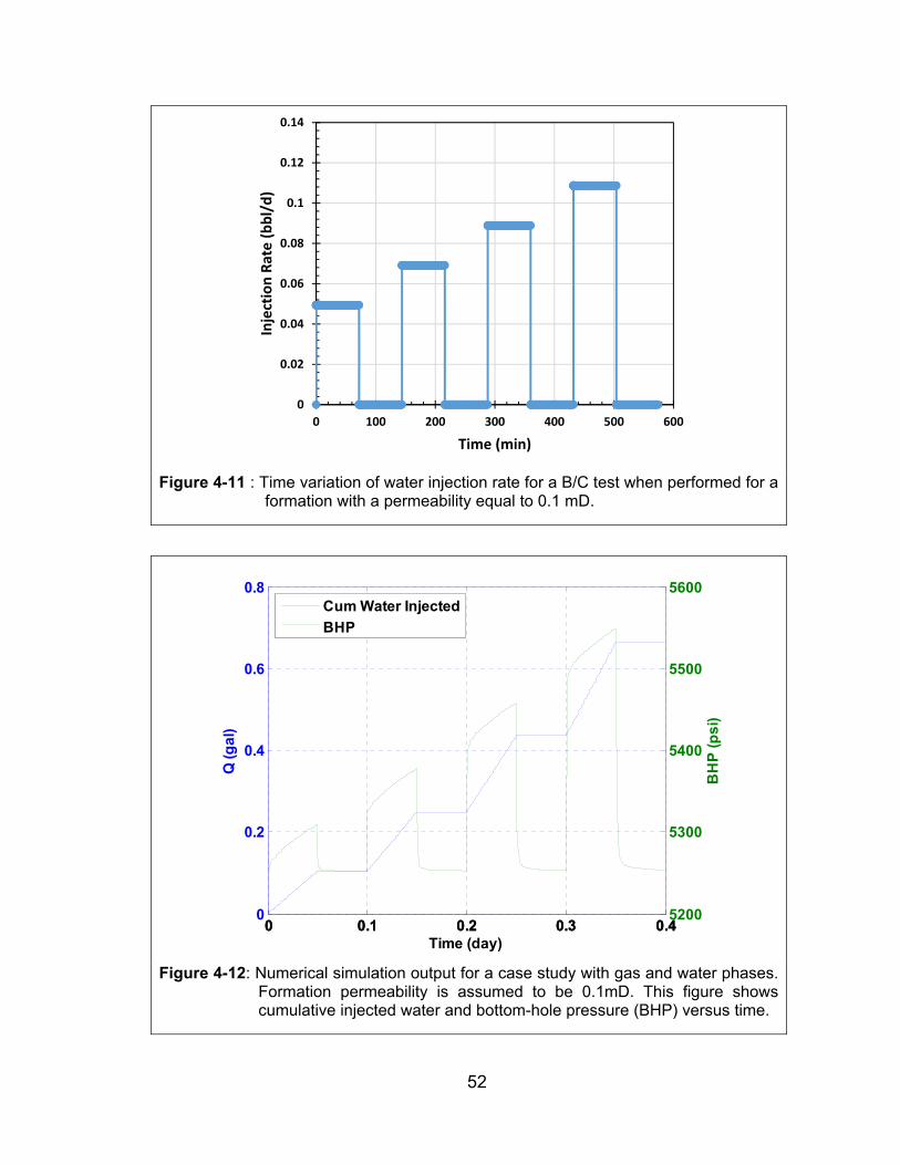
52

Figure 4-11 : Time variation of water injection rate for a B/C test when performed for a

formation with a permeability equal to 0.1 mD.

Figure 4-12: Numerical simulation output for a case study with gas and water phases. Formation permeability is assumed to be 0.1mD. This figure shows cumulative injected water and bottom-hole pressure (BHP) versus time.

0

0.02

0.04

0.06

0.08

0.1

0.12

0.14

0 100 200 300 400 500 600


Time (min)

0 0.1 0.2 0.3 0.40

0.2

0.4

0.6

0.8

Q (

ga

l)

Time (day)

0 0.1 0.2 0.3 0.45200

5300

5400

5500

5600

BH

P (p

si)

Cum Water Injected

BHP

53

Similar to Section 4.4.1, I plotted a graph of versus in

order to estimate alignment pressure for each pair. Figure 4-13 shows B/C

trends alignment for first, second, and third pairs. Table 4-2 summarizes

matching reservoir pressures, cumulative injected water, and average slope for

each pair of B/C trends at alignment.

Figure 4-13: Baseline/calibration alignment for a reservoir with 0.1 mD permeability. (a) First B/C pair is aligned at 5251 psi, (b) second B/C pair is aligned at 5252 psi, and (c) third B/C pair is aligned at 5253 psi.

0 20 40 60 800

0.2

0.4

0.6

0.8

1

1.2

1.4

Ln

(re

/rw

)


0 20 40 60 800

0.2

0.4

0.6

0.8

1

1.2

1.4

Ln

(re

/rw

)



0 20 40 60 800

0.2

0.4

0.6

0.8

1

1.2

1.4

Ln

(re

/rw

)


54


average slope for each pair of baseline/calibration trends. In this simulation, formation permeability is assumed to 0.1 mD.


1 0.104 5251.5 0.015

2 0.249 5252 0.0166

3 0.436 5253.2 0.016

Similar to Section 4.4.1, the baseline/calibration supercharging was

corrected by plotting calibrated baseline reservoir pressures versus cumulative

injected water. A linear trend line was drawn through matching pressure points,

and was extrapolated to zero cumulative water injection. Final estimation of

reservoir pressure is the pressure at zero cumulative injected water. In this

numerical case study, final estimate of reservoir pressure is 5250.9 psi with

0.017% error as shown in Figure 4-14.

It is observed that the percentage of error in this case study is lower in

comparison with the case study with permeability equal to 0.01 mD. This error is

due to the supercharging phenomena which is higher in lower permeability

reservoirs. Therefore the percentage of error is higher in the case study with

lower permeability.

55

Figure 4-14: Baseline/calibration supercharging correction for reservoir simulation with permeability 0.1 mD. A linear trend line was drawn through pressure match points and extrapolated to zero cumulative water injected. for the linear trend line is 0.97. The final estimate of reservoir pressure is 5250.9 psi.

Figure 4-15 compares the alignment matching pressure with calculated

average pressure of invaded zone. Alignment pressures agree well with

calculated average pressures at the end of each shut-in time. In this figure

alignment pressures are shown as blue points. Figure 4-16 shows the

agreement between average pressures of invaded area and alignment B/C

pressures as a function of time.

0 0.1 0.2 0.3 0.4 0.5 0.6 0.75250.5

5251

5251.5

5252

5252.5

5253

5253.5

5254

5254.5

Q (gal)

Pre

s (

ps

i)

Pr_final 5250.9

Error% 0.016978

Pr_final 5250.9

Error% 0.017

56

Figure 4-15: Average pressures of invaded zone versus cumulative injected water for a numerical simulation with permeability equal to 0.1 mD. Alignment Pressures have good agreement with average reservoir pressures at the end of shut-in times.

The maximum value of effective water permeability for this simulation

model is 0.03. Using Equation (2-62), calculated effective water permeability is

0.025 mD which represents the average effective permeability to water in the

radius of invasion. Using the rock-fluid properties, described in Figure 3-6, I

estimated gas effective permeability as

.

.∗ 0.025 0.067 .

Figure 4-17 shows water saturation distribution at the end of injection and shut-in

times.

0 0.1 0.2 0.3 0.4 0.5 0.6 0.75250

5255

5260

5265

5270

5275

5280

CumW

(Gal)

Pa

vg (

ps

i)

Avg Pr

Alignment Pressure

57

Figure 4-16: Average pressures versus time for a numerical simulation with

permeability 0.1 mD. Alignment pressures are approximately the same as average pressure of invaded zone at the end of shut-in times.


0 0.1 0.2 0.3 0.45250

5255

5260

5265

5270

5275

5280

Time (Day)

Pa

vg (

ps

i)

Avg Pr

Alignment Pressure

0.4 0.5 0.6 0.7 0.8 0.9 10.1

0.2

0.3

0.4

0.5

0.6

0.7

0.8


Wa

ter

Sa

tura

tio

n

Time = 72 min

Time = 144 min

Time = 216 min

Time = 288 min

Time = 360 min

Time = 432 min

Time = 504 min

Time = 576 min

58



in a numerical reservoir model with a formation permeability of 0.001 mD.

Reservoir and fluid properties are those described in Chapter 3. For the

simulation of this case study of B/C test, I injected of water in 4 discrete stages

as shown in Figure 4-18. Figure 4-19 shows the schedule of bottom-hole

pressure and cumulative injected water. As shown in this figure, I used lower

injection rates because formation permeability of this numerical simulation was

very low, and high injection rates might propagate a fracture.

Figure 4-18 : Time variation of injection rate for B/C test when performed for a formation with permeability equal to 0.001 mD.

0

0.005

0.01

0.015

0.02

0.025

0.03

0.035

0.04

0.045

0.05

0 100 200 300 400 500 600


Time (min)

59

Similar to Section 4.4.1, I plotted a graph of versus to

estimate alignment pressures for each pair of B/C trends. Figure 4-19 presents

B/C trends alignment for the first, second, and third pairs. Table 4-3 summarizes

matching reservoir pressures, cumulative injected water, and average slope for

each pair of B/C trends at alignment.

As described in Section 4.4.1, baseline/calibration supercharging is

corrected by plotting calibrated baseline reservoir pressures versus cumulative

injected water. I passed a linear trend line through alignment pressure points,

and extrapolated it to zero cumulative injected water. Final estimated reservoir

pressure is the pressure at zero cumulative injected water where reservoir is at

the initial condition. In this numerical case study, the final estimate of reservoir

pressure is 5260 psi with 0.19% error as shown in Figure 4-21.

It is observed that the percentage of error in this case in higher than that in

other cases. Since in this numerical simulation model, the assumed formation

permeability is lower than the previous two cases, the supercharging effect is has

higher impact in calculating initial reservoir pressure, and consequently, the error

is higher in this case study. However, the error of 0.19% is still very low, and less

than 1%.

60

Figure 4-19: Numerical simulation output for a reservoir with two phases of gas and water. Formation permeability is assumed to be 0.001mD. This figure shows cumulative water injected and bottom-hole pressure (BHP) versus time.

Figure 4-22 compares the alignment pressures with calculated average

pressures within the radius of invasion. Alignment pressures agree well with

calculated average pressures at the end of each shut-in time. Figure 4-23 shows

the agreement between average pressures and alignment B/C pressures as a

function of time.

0 0.05 0.1 0.15 0.2 0.25 0.3 0.35 0.40

0.2

0.4

Q (

ga

l)

Time (day)

0 0.05 0.1 0.15 0.2 0.25 0.3 0.35 0.4

5000

10000

Cum Water Injected

BHP

61

Figure 4-20: Baseline/calibration alignment for a case study with 0.001 mD permeability. (a) First B/C pair is aligned at 5271 psi, (b) second B/C pair is aligned at 5311 psi, and (c) third B/C pair is aligned at 5347 psi.


average slope for each pair of baseline/calibration trends. In this simulation, formation permeability is assumed to 0.001 mD.


1 0.021 5271 0.00014

2 0.062 5311 0.00016

3 0.125 5347.3 0.00015

0 1000 2000 3000 40000

0.1

0.2

0.3

0.4

0.5

0.6

0.7

Ln

(re

/rw

)


-1000 0 1000 2000 3000 40000

0.1

0.2

0.3

0.4

0.5

0.6

0.7

Ln

(re

/rw

)


-1000 0 1000 2000 3000 40000

0.2

0.4

0.6

0.8

Ln

(re

/rw

)



62

Figure 4-21: Baseline/calibration supercharging correction for reservoir simulation with permeability 0.001 mD. The linear trend line passes through pressure match points and extrapolated to zero cumulative water injected. of the linear trend line is 0.98. The final estimate of reservoir pressure is 5259.9psi.

Using Equation (2-62), calculated effective water permeability is 0.00024

mD. The maximum value of effective water permeability for this numerical

simulation model is 0.0003 mD. Calculated permeability of 0.00024 mD

represents the average effective permeability to water through the radius of

invasion. Using the rock-fluid properties, in Figure 3-6, I estimated gas effective

permeability as

.

.∗ 0.00024 0.00064 .

0 0.05 0.1 0.15 0.2 0.255240

5260

5280

5300

5320

5340

5360

5380

5400

5420

Q (gal)

Pre

s (

ps

i)

Pr_final 5259.9

Error% 0.188

63

Figure 4-24 shows water saturation distribution at the end of injection and shut-in

times.

Figure 4-22: Average pressures of invaded zone versus cumulative water injected for a numerical simulation with permeability 0.001 mD. The alignment pressures are approximately the same as average pressures at the end of shut-in times.

0 0.05 0.1 0.15 0.2 0.255250

5300

5350

5400

5450

5500

5550

5600

5650

CumW

(Gal)

Pa

vg (

ps

i)

Avg Pr

Alignment Pressure

64

Figure 4-23: Average pressures of invaded area versus time for a numerical simulation

with permeability 0.001 mD. Alignment pressures are approximately the same as average pressures at the end of shut-in times.

0 0.1 0.2 0.3 0.45250

5300

5350

5400

5450

5500

5550

5600

5650

Time (Day)

Pa

vg (

ps

i)

Avg Pr

Alignment Pressure

65


0.4 0.5 0.6 0.7 0.8 0.9 10.1

0.2

0.3

0.4

0.5

0.6

0.7

0.8


Wa

ter

Sa

tura

tio

n

Time = 72 min

Time = 144 min

Time = 216 min

Time = 288 min

Time = 360 min

Time = 432 min

Time = 504 min

Time = 576 min

66

Field Trial Applications

5.1 Introduction

Baseline/calibration technique has been tested on several wells in the

Almond formation of Wamsutter field, Wyoming. These wells are operated and

B/C tests were performed by BP. In two of the wells studied, downhole gauges

were used to measure sandface pressure and flow rate with high quality. Using

downhole gauges in these two wells provided the opportunity to investigate the

difference between surface and downhole pressures. The effect of gas influx,

pressure gradient, and frictional pressure drop were calculated for conversion of

pressure and injection rate from surface to sandface condition. In this study, I

used the sandface pressure and injection rate data provided by BP

unconventional gas flagship. The operator has converted surface flow rate and

pressure to those in sandface condition.

The most practical and operational cost effective protocol for a B/C test is

Falling Fluid Level Test (FFLT1) protocol. Through a FFLT, it is possible to use

surface gauges and therefore performing B/C test becomes more cost effective.

FFLT is BP’s desirable protocol to conduct a B/C test. However, BP has also

tested the B/C method using Constant Pressure Injection Test (CPIT2) and

1 FFLT consists of injection by changing sandface rate and pressure at the same time. 2 CPIT consists of injection at a constant bottom-hole pressure followed by a short shut-in time.

67

Constant Rate Injection Test (CRIT3) protocols. Performing a B/C test using a

CPIT or CRIT protocol is less practical and more expensive in comparison to

FFLT due to the need for a separate and special system to keep the sandface

pressure or injection rate constant. BP has tested B/C method using CPIT and

CRIT less frequently and FFLT more frequently.

In this chapter, I evaluated sandface pressure and injection rate data

obtained from B/C tests, performed on two Wamsutter wells. I estimated

reservoir pressure value using the method described in Chapter 2.

5.2 Field Trial One

In this field trial, baseline/calibration test is performed using a FFLT. Water

was injected in 4 different injection stages as shown in Figure 5-1. In this field

trial, water was injected for approximately 30 minutes in each stage followed by 2

minutes shut-in. Figure 5-2 demonstrates the time variation of sandface pressure

and cumulative injected water.

During early stages of completion, when a B/C test is conducted,

information such as porosity, initial water saturation, residual gas saturation, and

reservoir height are not available. According to Equation (2-51),

5.615

1. (2-51)

Assuming constant height, porosity, initial water saturation, and residual gas

saturation, then ln is proportional to . Therefore, a graph of

3 CRIT consists of injection at a constant flow rate while bottom-hole pressure is variable.

68

ln versus Δ / can be used to find alignment pressure for each injection pair.

Figure 5-3 shows B/C trend alignment between different stages of the test trial.

Figure 5-1: Time variation of injection rate during baseline/calibration field trial one. This test was conducted with FFLT protocol.

Table 5-1 summarizes the alignment reservoir pressures and cumulative

injected water for each B/C pair. Figure 5-4 shows that supercharging correction

is applied to find final estimate of reservoir pressure as 4585 psi.

0

0.5

1

1.5

2

2.5

3

3.5

4

4.5

5

0 1 2 3 4 5

Injection Rate (BPD)

Time (Hour)

Stage 1

Stage 2

Stage 3

Stage 4

69

Figure 5-2: Cumulated injected water and sandface pressure during baseline/calibration field trial one.

Table 5-1: Summary of cumulative injected water and alignment reservoir pressure for each baseline/calibration trend, field trial one.

Pair Q (gal) Pr-match (psi)

1 2.692 4850

2 4.127 5050

3 5.991 5200

4700

4900

5100

5300

5500

5700

5900

6100

0

1

2

3

4

5

6

7

8

9

0 1 2 3 4 5

Pressure (Psi)

Cum. W

ater Injected (Gal)

Time (hour)

Cum. Injected WaterSandface Pressure

70

(a) Stage one and stage two of trend lines are aligned at pressure equal to 4850 psi.

(b) Stage two and stage three of trend lines are aligned at pressure equal to 5050 psi.

(c) Stage three and stage four of trend lines are aligned at pressure equal to 5200 psi.

Figure 5-3: Baseline/calibration trend alignment for the field trial one. (a) First pair is aligned at 4850 , (b) second pair is aligned at 5050 , and (c) third pair is aligned at 5200 .

0

0.5

1

1.5

2

2.5

0 5 10 15

LN(Q) (Gal)

dp/q (Psi/GPD)

0

0.5

1

1.5

2

2.5

‐5 0 5 10 15

LN(Q) (Gal)

dp/q (Psi/GPD)

0

0.5

1

1.5

2

2.5

‐10 ‐5 0 5 10

LN(Q) (Gal)

dp/q (Psi/GPD)

71

Figure 5-4: Supercharging correction for baseline/calibration field trial one. A linear trend line passes through pressure points and extrapolates to zero cumulative water injected. for this linear trend line is 0.97.

5.3 Field Trial Two

In this section, I analyzed the pressure and injection rate data from

another baseline/calibration field trial performed with a FFLT protocol. Water was

injected in 4 discrete stages as shown in Figure 5-5. Each injection stage lasted

approximately 15 minutes followed by 3 minutes of shut-in. Figure 5-6 presents

the schedule of sandface pressures and cumulative injected water values.

Figure 5-7 shows B/C trend alignment between different stages of the test

trial. Alignment pressures and cumulative injected water for each pair are

summarized in Table 5-2.

4500

4600

4700

4800

4900

5000

5100

5200

5300

0 1 2 3 4 5 6 7

Pr_Match (Psi)

Q (Gal)

72

Figure 5-5: Time variation of injection rate during baseline/calibration field trial two. This test was conducted with FFLT protocol.

Figure 5-6: Cumulated injected water and sandface pressure during baseline/calibration field trial two.

0

10

20

30

40

50

60

0 0.2 0.4 0.6 0.8 1 1.2

Injection Rate (BPD)

Time (Hour)

Stage 1

Stage 2

Stage 3

Stage 4

4500

4700

4900

5100

5300

5500

5700

5900

6100

6300

0

2

4

6

8

10

12

14

16

0 0.2 0.4 0.6 0.8 1 1.2

Pressure (Psi)

Cum. W

ater Injected (Gal)

Time (Hour)

Cum. Injected WaterSandface Pressure

73

The supercharge correction was applied to determine the final estimate of

reservoir pressure as shown in Figure 5-8. Reservoir pressure was calculated to

be 4930 psi in this field trial.

Table 5-2: Summary of cumulative injected water and alignment reservoir pressure for each baseline/calibration trend, field trial two.

Pair Q (gal) Pr-match (psi)

1 0.632 4900

2 2.203 5325

3 6.195 5600

74

(a) Stage one and stage two of trend lines are aligned at pressure equal to 4900 psi.

(b) Stage two and stage three of trend lines are aligned at pressure equal to 5325 psi.

(c) Stage three and stage four of trend lines are aligned at pressure equal to 5600 psi.

Figure 5-7: Baseline/calibration trend alignment for the field trial two. (a) First pair is aligned at 4900 , (b) second pair is aligned at 5325 , and (c) third pair is aligned at 5600 .

‐2.5

‐2

‐1.5

‐1

‐0.5

0

0.5

1

1.5

2

2.5

3

0 2 4 6 8

LN(Q) (Gal)

dp/q (Psi/GPD)

Stage 1

Stage 2

Stage 3

Stage 4‐2.5

‐2

‐1.5

‐1

‐0.5

0

0.5

1

1.5

2

2.5

3

‐15 ‐10 ‐5 0 5

LN(Q) (Gal)

dp/q (Psi/GPD)

Stage 1

Stage 2

Stage 3

Stage 4

‐2.5

‐2

‐1.5

‐1

‐0.5

0

0.5

1

1.5

2

2.5

3

‐30 ‐20 ‐10 0 10

LN(Q) (Gal)

dp/q (Psi/GPD)

Stage 1

Stage 2

Stage 3

Stage 4

75

Figure 5-8: Supercharge correction for baseline/calibration field trial two. A linear trend line passes through pressure points and extrapolates to zero cumulative water injected. for this linear trend line is 0.87.

4800

4900

5000

5100

5200

5300

5400

5500

5600

5700

0 1 2 3 4 5 6 7

Pr_Match (psi)

Q (Gal)

76

Summary and Conclusions

I developed the mathematical basis for a new and operationally cost

effective approach, called baseline/calibration, to estimate formation pressure

and effective water permeability. I derived and successfully validated

mathematical formulations for pressure variations during a baseline/calibration

test. These mathematical formulations were based on (i) the line-source solution

to the diffusivity equation, (ii) the principle of superposition in time, and (iii) the

approximately piston-like displacement of injected water. The derived

mathematical formulation verified that each pair of trends should be aligned

linearly at a specific pressure. The alignment pressure for each pair was found to

be the average pressure of invaded area at the onset of corresponding injection

stage. I presented a method to correct for supercharging effect and determined

final estimated reservoir pressure.

I constructed several numerical reservoir simulation models to validate

baseline/calibration technique. These models included different representative

petrophysical rock types for tight gas sand formations of Wamsutter field. Using

the baseline/calibration method, initial reservoir pressure was estimated

accurately for all numerical simulation models. The range of error in calculated

reservoir pressure for these models was from 0.017% to 0.188%. I observed that

the percentage of error was higher in formations with lower permeability.

77

Accuracy of pressure estimates was reduced in tight formations due to a more

significant supercharging.

I developed and validated a new approach to estimate effective

permeability to water. Simulation results showed calculated effective water

permeability agreed well with actual effective water permeability.

The results of numerical simulations and field trials showed that the

baseline/calibration method can be successful in estimating formation pressure in

very short test times.

78

References

Abdollah-Pour, R. 2011. Development and Application of a 3D Equation-of-State

Compositional Fluid-Flow Simulator in Cylindrical Coordinates for Near-Wellbore

Phenomena. Ph.D., University of Texas at Austin, Texas, USA.

Adams, J.R., Dotson, B., Sebastian, H., and Motealleh, S. 2013.

Baseline/Calibration Method for Reservoir Pressure Determination. Presented at

the SPE Unconventional Resources Technology Conference, Denver, Colorado,

12-14 August, SPE-168900-MS. http://dx.doi.org/10.1190/URTEC2013-022.

Adams, J.R., Motealleh, S., Sebastian, H., Jiang, Y., and Dotson, B. 2012.

Method of Determining Reservoir Pressure. USA Patent No.

Agarwal, R.G., Al-Hussainy, R., and Ramey Jr., H.J. 1965. The Importance of

Water Influx in Gas Reservoirs. Journal of Petroleum Technology 17 (11): 1336-

1342. SPE-1244-PA. http://dx.doi.org/10.2118/1244-PA.

Cramer, D.D. and Nguyen, D.H. 2013. Diagnostic Fracture Injection Testing

Tactics in Unconventional Reservoirs. Presented at the SPE Hydraulic Fracturing

Technology Conference, The Woodlands, Texas, 4-6 February, SPE-163863-

MS. http://dx.doi.org/10.2118/163863-MS.

79

Economides, M.J., Hill, A.D., Economides, C.E., and Zhu, D. . 2013. Petroleum

Production Systems, second edition. Westford, Masscachusetts: Pearson

Education.

Geffen, T.M., Parrish, D.R., Haynes, G.W., and Morse, R.A. 1952. Efficiency of

Gas Displacement From Porous Media by Liquid Flooding. Journal of Petroleum

Technology 4 (02): 29-38. SPE-952029-G. http://dx.doi.org/10.2118/952029-G.

Jin, M., Zhang, W., and Zhang, H. 2013. Integrated Well Test Strategy in

Unconventional Tight Gas Reservoirs-Learning and Experiences from an Actual

Field Project. Presented at the International Petroleum Technology Conference,

Beijing, China, 26-28 March, IPTC-16950-Abstract.

http://dx.doi.org/10.2523/16950-ABSTRACT.

Lee, J., Rollins, J.B., and Spivey, J.P. 2003. Pressure Transient Testing, first

edition. Richardson, Texas: Society of Petroleum Engineers.

Martin, A.R., Cramer, D.D., Nunez, N., and Roberts, N.R. 2013. A Method to

Perform Multiple Diagnostic Fracture Injection Tests Simultaneously in a Single

Wellbore. SPE Production & Operations 28 (02): 91-200. SPE-152019-PA.

http://dx.doi.org/10.2118/152019-PA.

80

Martin, J.C. 1959. The Simplified Equations of Flow in Gas Drive Reservoirs and

the Theoretical Foundation of Multiphase Pressure Buildup Analyses. Society of

Petroleum Engineers 216. SPE 1235-G.

Matthews, C.S. and Russell, D.G. 1967. Pressure Buildup and Flow Tests in

Wells, first edition. Dallas, Texas: Society of Petroleum Engineers.

Merletti, G.D., Abdollah-Pour, R., and Spain, D.R. 2013. Calibration of Static

Reservoir Models with Dynamic Data for Efficient Tight-Gas Field Development

(Wyoming, US). Presented at the SPE Unconventional Gas Conference and

Exhibition,, Muscat, Oman, 28-30 January, SPE-164031-MS.

http://dx.doi.org/10.2118/164031-MS.

Peters, E.J. 2012. Advanced Petrophysics, first edition, Vol. 2. Austin, Texas:

Live Oak Book Company.

Satter, A., Igbal, G.M., and Buchwalter, J.L. 2008. Practical Enhanced Reservoir

Engineering, first edition. Tulsa, Oklahoma: PennWell Corporation.

Soliman, M. Y. and Kabir, C. S. 2012. Testing Unconventional Formations.

Journal of Petroleum Science and Engineering 92-93: 102-109.

http://dx.doi.org/10.1016/j.petrol.2012.04.027.

81

Soliman, M.Y. 1986. Analysis of Buildup Tests With Short Producing Time. SPE

Formation Evaluation 1 (04): 363-371. SPE-11083-PA.

http://dx.doi.org/10.2118/11083-PA.

Soliman, M.Y., Craig, D., Bartko, K., Rahim, Z., Ansah, J., and Adams, D. 2005.

New Method for Determination of Formation Permeability, Reservoir Pressure,

and Fracture Properties from a Minifrac Test Presented at the 40th U.S.

Symposium on Rock Mechanics (USRMS), Anchorage, Alaska, 25-29 June,

ARMA-05-658.

Soliman, M.Y., Shahri, M., and Lamei, H. 2013. Revisiting the Before Closure

Analysis Formulations in Diagnostic Fracturing Injection Test. Presented at the

SPE Hydraulic Fracturing Technology Conference, The Woodlands, Texas, 4-6

February, SPE-163869-MS. http://dx.doi.org/10.2118/163869-MS.

© Copyright by Zoha Nasizadeh, 2014

Documents

Transcript of © Copyright by Zoha Nasizadeh, 2014