orbilu.uni.luorbilu.uni.lu/bitstream/10993/13645/1/PM_Thalm_Wang.pdf · Bull. Sci. math. 135 (2011)...

Bull. Sci. math. 135 (2011) 816–843www.elsevier.com/locate/bulsci

A stochastic approach to a priori estimates andLiouville theorems for harmonic maps ✩

Anton Thalmaier a,∗, Feng-Yu Wang b,c

a Unité de Recherche en Mathématiques, FSTC, Université du Luxembourg, 6, rue Richard Coudenhove-Kalergi,L-1359, Luxembourg

b School of Mathematical Sciences, Beijing Normal University, Beijing, 100875, Chinac Department of Mathematics, Swansea University, Singleton Park, SA2 8PP, UK

Available online 8 July 2011

To the memory of Paul Malliavin

Abstract

Nonlinear versions of Bismut type formulas for the differential of a harmonic map between Riemannianmanifolds are used to establish a priori estimates for harmonic maps. A variety of Liouville type theoremsis shown to follow as corollaries from such estimates by exhausting the domain through an increasing se-quence of geodesic balls. This probabilistic method is well suited for proving sharp estimates under variouscurvature conditions. We discuss Liouville theorems for harmonic maps under the following conditions:small image, sublinear growth, non-positively curved targets, generalized bounded dilatation, Liouvillemanifolds as domains, certain asymptotic behaviour.© 2011 Elsevier Masson SAS. All rights reserved.

MSC: 58J65; 58J35; 60H30

Keywords: Liouville theorem; Harmonic map; Gradient estimate; Ricci curvature; Stochastic development; Brownianmotion; Nonlinear martingale; Bismut formula

✩ Supported in part by WIMCS, SRFDP, the Fundamental Research Funds for the Central Universities, and the FondsNational de la Recherche Luxembourg.

* Corresponding author.E-mail addresses: [email protected] (A. Thalmaier), [email protected] (F.-Y. Wang).

0007-4497/$ – see front matter © 2011 Elsevier Masson SAS. All rights reserved.doi:10.1016/j.bulsci.2011.07.014

A. Thalmaier, F.-Y. Wang / Bull. Sci. math. 135 (2011) 816–843 817

1. Introduction

In 1984 Bismut [4] established a derivative formula for the heat kernel on a Rieman-nian manifold in terms of an expectation (with respect to the Brownian bridge measure)of explicit curvature terms. Since then Bismut’s formula has been extended and applied invarious directions. The authors [32] obtained explicit gradient estimates of harmonic func-tions on regular domains by using the localized version of a Bismut type formula developedin [31].

The purpose of this paper is twofold: first we like to present estimates analogous to [32] inthe nonlinear setting of harmonic maps. To this end, we investigate a nonlinear version of thederivative formula, first established by Arnaudon and Thalmaier [3].

The second aim is to demonstrate the new method and to give simple proofs of various Li-ouville type theorems for harmonic maps by exploiting derivative estimates obtained from thenonlinear Bismut formula. It is not our main concern to prove new results, rather than to uncoverthe way how probability and geometry work together to enforce triviality for harmonic mapsin certain situations. The new probabilistic method is well suited to separate the influence ofcurvature conditions on the domain and on the target, in establishing sharp estimates in variousspecific situations.

A Liouville theorem is a statement of the form that under certain curvature conditions ondomain and target all harmonic maps u in a certain mapping class are necessarily constant, seefor instance [8,23], as well as [10] for estimates. Roughly speaking, Liouville theorem maybe classified into two categories: those requiring a restriction on the size of u(M), and thosewhere the condition on u is expressed in terms of the growth rate of the energy of u on geodesicballs.

The traditional probabilistic approach to Liouville type theorems is typically concerned withnon-existence of certain types of harmonic maps by verifying that, under the given constraints,such maps would link random processes on the domain and the target in an incompatible way,see for instance [16] for an account in this direction. A stochastic approach along these lineshas been applied by S. Stafford [29] to prove S.-Y. Cheng’s Liouville theorem [5]. Probabilisticmethods relying on coupling of Brownian motions on Riemannian manifolds have been used byF.-Y. Wang [33]. See also J. Picard [22].

Our approach here is quite different: We start from an exact Bismut type expression for thedifferential of a harmonic map. This formula is exploited under the given curvature conditions toderive precise estimates on certain domains, like on geodesic balls. Since the underlying tool isan exact formula in a general setting, it is not surprising that the method can be adapted to dealwith quite a variety of different situations, as will be shown in Section 5; there is also no doubtthat this approach can be used to prove many other results in this direction. It can be seen as aunifying approach to a priori estimates for harmonic maps.

The paper is organized as follows. In Section 2 we collect some basic estimates for geodesictransports along semimartingales and in Section 3 we recall the nonlinear derivative formulaobtained in [3]. To follow the lines of [32], a variant of the formula is presented in Theorem 3.3.In Section 4 we estimate the first-order differential of harmonic maps via lower bounds of theRicci curvature on the domain manifold and upper bounds of the sectional curvatures on thetarget. Finally, in Section 5, Liouville type theorems for harmonic maps are deduced from ourderivative estimates in a variety of different situations.

818 A. Thalmaier, F.-Y. Wang / Bull. Sci. math. 135 (2011) 816–843

2. Geodesic transports

Definition 2.1 (Geodesic transport along a semimartingale). Let (N,h) be a Riemannian man-ifold and Y be a continuous semimartingale taking values in N . The geodesic transport (alsocalled damped or deformed parallel transport [3])

Θ0,t :TY0N → TYt N

along Y is defined by the following covariant equation along Y :

d(//−1

0,. Θ0,.)= −1

2//−1

0,. RN(Θ0,., dY )dY with Θ0,0 = id, (2.1)

where RN denotes the Riemann curvature tensor on N .

Example 2.2 (Geodesic transport along a Brownian motion). Let Y be Brownian motion on(N,h). Then Eq. (2.1) reduces to

d(//−1

0,. Θ0,.)= −1

2//−1

0,. RicN(Θ0,s) ds with Θ0,0 = id,

where RicN is the Ricci curvature of N . We use the convention RicN ∈ Γ (End(T N)), i.e.,RicN :TxN → TxN for each x ∈ N , RicN(v) ≡ RicN

x (v, ·)#.

Definition 2.3 (Anti-development). Let Y be a continuous semimartingale taking values in a Rie-mannian manifold N . The TY0N -valued processes A (Y ), resp. Adef(Y ), defined by the followingStratonovich integrals,

A (Y ) :=.∫

0

//−10,s δYs, Adef(Y ) :=

.∫0

Θ−10,s δYs, (2.2)

are called the anti-development of Y , resp. deformed anti-development of Y .

Remarks 2.4. a) The notion of the geodesic transport (Definition 2.1), as well as the notion ofanti-development (Definition 2.3), requires a differentiable manifold endowed with a connection;the Riemannian structure is not needed. However, since we only deal with the Levi–Civita con-nection on a Riemannian manifold, this point will not be important for us. In the sequel ∇ alwaysdenotes the Levi–Civita connection.

b) In Eq. (2.2) the Stratonovich integrals with respect to δYs can be replaced by Ito integralswith respect to d∇Ys as well, see [3] for details.

c) A continuous semimartingale Y on (N,h) is a ∇-martingale if and only if A (Y ), or equiv-alently Adef(Y ), is a local martingale in TY0N .

d) A continuous semimartingale Y on (N,h) is a Brownian motion if and only if A (Y ) is aBrownian motion in TY0N .

In the following let (N,h) be a Riemannian manifold and Y be a continuous semimartingaletaking values in N . Let Z := A (Y ) be the anti-development of Y and

∫h(dY,dY ) its Rieman-

nian quadratic variation. Then

h(dY,dY ) = traced[Z,Z] =n∑

d[Zi,Zi

]
i=1


with respect to any orthonormal basis of TY0N . Consider the End(TY0N)-valued process Λ given(with respect to an arbitrary orthonormal basis of TY0N ) by the n × n matrix

Λjk := d[Zj ,Zk]h(dY,dY )

, 1 � j, k � n

(defined as Radon–Nikodym derivative for h(dY,dY )-almost all t , and by 0 else).

Definition 2.5 (Semimartingales of bounded dilatation). Let Y be a continuous semimartingaletaking values in a Riemannian manifold N . We say that Y is of generalized K-bounded dilatation(e.g. [16]) if P-almost surely,

λ1(t) � K2(λ2(t) + · · · + λn(t))

(2.3)

holds for some K > 0 and all t ∈ R+, where

λ1(t) � λ2(t) � · · · � λn(t) � 0 (2.4)

denotes the eigenvalues of Λt . The semimartingale Y is said to be K-quasi-conformal, if λ1(t) �K2λn(t) instead of condition (2.3) holds for all t � 0.

The following lemma is an extension of Proposition 2.8 in [2], and gives the basic estimatesfor the geodesic transport along a semimartingale in terms of the quadratic variation. We use thenotation

(sup Sect)(y) = supremum of the sectional curvatures of N at y,

(inf Sect)(y) = infimum of the sectional curvatures of N at y

for any y ∈ N .

Lemma 2.6. Let Θ0,. :TY0N → TY.N be the geodesic transport along a continuous semimartin-gale Y in (N,h) and let

Θs,t := Θ0,t ◦ Θ−10,s :TYs N → TYt N.

Then for any 0 � s � t the following estimates hold:

exp

(−1

2

t∫s

Lr h(dYr , dYr)

)� |Θs,t | � exp

(−1

2

t∫s

�r h(dYr , dYr)

)(2.5)

where

Lr :={

(sup Sect)(Yr) if (sup Sect)(Yr) � 0,

[λ2(r) + · · · + λn(r)](sup Sect)(Yr) if (sup Sect)(Yr) � 0,(2.6)

respectively,

�r :={

(inf Sect)(Yr) if (inf Sect)(Yr) � 0,

[λ2(r) + · · · + λn(r)](inf Sect)(Yr ) if (inf Sect)(Yr) � 0.(2.7)

Here the λi(r) are as in Definition 2.5.


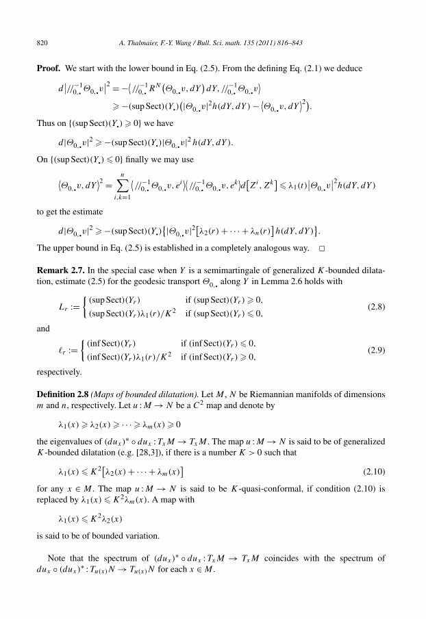
Proof. We start with the lower bound in Eq. (2.5). From the defining Eq. (2.1) we deduce

d∣∣//−1

0,. Θ0,.v∣∣2 = −⟨//−1

0,. RN(Θ0,.v, dY

)dY, //−1

0,. Θ0,.v⟩

� −(sup Sect)(Y.)(|Θ0,.v|2h(dY,dY ) − ⟨Θ0,.v, dY

⟩2).

Thus on {(sup Sect)(Y.) � 0} we have

d|Θ0,.v|2 � −(sup Sect)(Y.)|Θ0,.v|2 h(dY,dY ).

On {(sup Sect)(Y.) � 0} finally we may use

⟨Θ0,.v, dY

⟩2 =n∑

i,k=1

⟨//−1

0,. Θ0,.v, ei⟩⟨//−1

0,. Θ0,.v, ek⟩d[Zi,Zk

]� λ1(t)

∣∣Θ0,.v∣∣2h(dY,dY )

to get the estimate

d|Θ0,.v|2 � −(sup Sect)(Y.){|Θ0,.v|2[λ2(r) + · · · + λn(r)

]h(dY,dY )

}.

The upper bound in Eq. (2.5) is established in a completely analogous way. �Remark 2.7. In the special case when Y is a semimartingale of generalized K-bounded dilata-tion, estimate (2.5) for the geodesic transport Θ0,. along Y in Lemma 2.6 holds with

Lr :={

(sup Sect)(Yr) if (sup Sect)(Yr) � 0,

(sup Sect)(Yr)λ1(r)/K2 if (sup Sect)(Yr) � 0,

(2.8)

and

�r :={

(inf Sect)(Yr ) if (inf Sect)(Yr ) � 0,

(inf Sect)(Yr )λ1(r)/K2 if (inf Sect)(Yr ) � 0,

(2.9)

respectively.

Definition 2.8 (Maps of bounded dilatation). Let M , N be Riemannian manifolds of dimensionsm and n, respectively. Let u :M → N be a C2 map and denote by

λ1(x) � λ2(x) � · · · � λm(x) � 0

the eigenvalues of (dux)∗ ◦ dux :TxM → TxM . The map u :M → N is said to be of generalized

K-bounded dilatation (e.g. [28,3]), if there is a number K > 0 such that

λ1(x) � K2[λ2(x) + · · · + λm(x)]

(2.10)

for any x ∈ M . The map u :M → N is said to be K-quasi-conformal, if condition (2.10) isreplaced by λ1(x) � K2λm(x). A map with

λ1(x) � K2λ2(x)

is said to be of bounded variation.

Note that the spectrum of (dux)∗ ◦ dux :TxM → TxM coincides with the spectrum of

dux ◦ (dux)∗ :Tu(x)N → Tu(x)N for each x ∈ M .


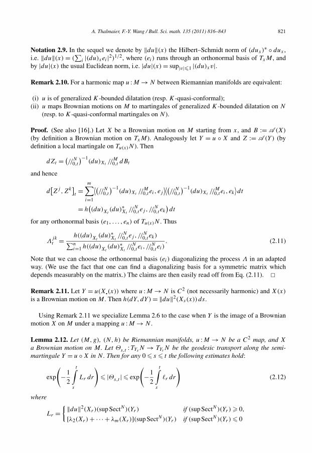
Notation 2.9. In the sequel we denote by ‖du‖(x) the Hilbert–Schmidt norm of (dux)∗ ◦ dux ,

i.e. ‖du‖(x) = (∑

i |(du)xei |2)1/2, where (ei) runs through an orthonormal basis of TxM , andby |du|(x) the usual Euclidean norm, i.e. |du|(x) = sup|v|�1 |(du)xv|.

Remark 2.10. For a harmonic map u :M → N between Riemannian manifolds are equivalent:

(i) u is of generalized K-bounded dilatation (resp. K-quasi-conformal);(ii) u maps Brownian motions on M to martingales of generalized K-bounded dilatation on N

(resp. to K-quasi-conformal martingales on N ).

Proof. (See also [16].) Let X be a Brownian motion on M starting from x, and B := A (X)

(by definition a Brownian motion on TxM). Analogously let Y = u ◦ X and Z := A (Y ) (bydefinition a local martingale on Tu(x)N ). Then

dZt = (//N0,t

)−1(du)Xt //

M0,t dBt

and hence

d[Zj ,Zk

]t=

m∑i=1

⟨(//N

0,t

)−1(du)Xt //

M0,t ei , ej

⟩⟨(//N

0,t

)−1(du)Xt //

M0,t ei , ek

⟩dt

= h((du)Xt

(du)∗Xt//N

0,t ej , //N0,t ek

)dt

for any orthonormal basis (e1, . . . , en) of Tu(x)N . Thus

Λjkt = h((du)Xt

(du)∗Xt//N

0,t ej , //N0,t ek)∑n

i=1 h((du)Xt(du)∗Xt

//N0,t ei , //

N0,t ei)

. (2.11)

Note that we can choose the orthonormal basis (ei) diagonalizing the process Λ in an adaptedway. (We use the fact that one can find a diagonalizing basis for a symmetric matrix whichdepends measurably on the matrix.) The claims are then easily read off from Eq. (2.11). �Remark 2.11. Let Y = u(X.(x)) where u :M → N is C2 (not necessarily harmonic) and X(x)

is a Brownian motion on M . Then h(dY,dY ) = ‖du‖2(Xs(x)) ds.

Using Remark 2.11 we specialize Lemma 2.6 to the case when Y is the image of a Brownianmotion X on M under a mapping u :M → N .

Lemma 2.12. Let (M,g), (N,h) be Riemannian manifolds, u :M → N be a C2 map, and X

a Brownian motion on M . Let Θs,t :TYs N → TYt N be the geodesic transport along the semi-martingale Y = u ◦ X in N . Then for any 0 � s � t the following estimates hold:

exp

(−1

2

t∫s

Lr dr

)� |Θs,t | � exp

(−1

2

t∫s

�r dr

)(2.12)

where

Lr ={‖du‖2(Xr)(sup SectN)(Yr) if (sup SectN)(Yr) � 0,

N N
[λ2(Xr) + · · · + λm(Xr)](sup Sect )(Yr) if (sup Sect )(Yr) � 0


and

�r ={‖du‖2(Xr)(inf SectN)(Yr) if (inf SectN)(Yr) � 0,

[λ2(Xr) + · · · + λm(Xr)](inf SectN)(Yr) if (inf SectN)(Yr) � 0

and with λi(x) as in Definition 2.8.

Remark 2.13. In the special case when u is a map of generalized K-bounded dilatation, esti-mate (2.12) for the geodesic transport Θ0,. holds with

Lr ={‖du‖2(Xr)(sup SectN)(Yr) if (sup SectN)(Yr) � 0,

(sup SectN)(Yr)λ1(Xr)/K2 if (sup SectN)(Yr) � 0

and

�r ={‖du‖2(Xr)(inf SectN)(Yr) if (inf SectN)(Yr) � 0,

(inf SectN)(Yr)λ1(Xr)/K2 if (inf SectN)(Yr) � 0.

Note that λ1(x) = |du|2(x).

Remark 2.14. We always have the obvious estimate

exp

(−1

2

t∫s

κ+(Yr)‖du‖2(Xr) dr

)� |Θs,t | � exp

(−1

2

t∫s

κ−(Yr)‖du‖2(Xr), dr

)

where κ+(y) := (sup SectN)(y) ∨ 0 and κ−(y) := inf SectN(y) ∧ 0.

3. Derivative formulas for harmonic maps

To formulate derivative formulas for harmonic maps, we consider the following setup. Letu :M → N be a C2 map between two Riemannian manifolds. Further let X.(x) be a Brownianmotion on M , starting from x, and let Y := u(X(x)) be its image process under u on N , startingfrom u(x). Let ΘM

0,. denote the geodesic transport on M along X.(x), and ΘN0,. the corresponding

transport on N along Y . Finally let B := A (X(x)) = ∫0 //−10,s δXs(x) be the anti-development

of X(x), by definition a Brownian motion on TxM , and let Adef(Y ) = ∫0(ΘN0,s )

−1δYs be thedeformed anti-development of Y .

Theorem 3.1 (Basic derivative formula for harmonic maps). (Cf. [3], Section 5.) Let (M,g)

and (N,h) be Riemannian manifolds and u ∈ C2(M,N). Let x ∈ M and let D be a relativelycompact open neighbourhood of x in M . Suppose that u is harmonic on D. Then Y = u(X.(x))

is a ∇-martingale on N up to the first exit time τ(x) of X.(x) from D. For any v ∈ TxM thefollowing formula holds:

(du)xv = −E

[Adef(Y )τ

τ∫0

⟨ΘM

0,s �(s), //M0,s dBs

⟩](3.1)


where τ is any bounded stopping time such that 0 < τ � τ(x) and � is any adapted process withfinite energy taking values in TxM such that

(i) �(0) = v and �(s) = 0 for s � τ ,(ii) (∫ τ

0 |�(s)|2 ds)1/2 ∈ L1+ε for some ε > 0.

Sketch of the proof. We briefly recall the idea behind Theorem 3.1. First one shows that{(ΘN

0,s

)−1(du)Xs(x)Θ

M0,s : s < τ(x)

}(3.2)

is a local martingale in TxM ⊗ Tu(x)N , see [3], Section 5. Hence also

ns := (ΘN0,s

)−1(du)Xs(x)Θ

M0,s�(s) −

s∫0

(ΘN

0,r

)−1(du)Xr(x)Θ

M0,r �(r) dr (3.3)

is a local martingale up to the random time τ(x). Thus taking into account that

Adef(Y ) =∫0

(ΘN

0,s

)−1(du)Xs(x)//

M0,s dBs

we see that {ms : s < τ(x)} where

ms := (ΘN0,s

)−1(du)Xs(x)Θ

M0,s�(s) − Adef(Y )s

s∫0

⟨ΘM

0,r �(r), //M0,r dBr

⟩(3.4)

is a local martingale as well. The proof is completed by verifying that the local martingale {ms∧τ :s � 0} is a uniformly integrable martingale under the given assumptions. Formula (3.1) thenfollows by taking expectations: E[m0] = E[mτ ]. �

Note that formula (3.1) holds true for any stopping time τ and any finite energy process �

which meet the given constraints. It will be essential for our applications to deal with specificchoices for �. For further reference, we recall a general scheme for constructing appropriate finiteenergy processes, see [32].

Remark 3.2 (Construction of finite energy processes). Let D ⊂ M be a relatively compactopen domain with nonempty smooth boundary, and choose f ∈ C2(D) with f > 0 in D andf |∂D = 0. Let

σ(s) = inf

{r � 0:

r∫0

f −2(Xu(x))du � s

}(3.5)

be the time change as defined at the beginning of Section 4 in [32]. (Note that σ(s) is denotedτ(s) in [32].) We fix t > 0 and let

h0(s) =s∫

0

f −2(Xr(x))1{r<σ(t)} dr. (3.6)

Finally let h(s) = (h1 ◦ h0)(s) where h1 ∈ C1[0, t] such that h1(0) = 1, h1(t) = 0, h1 � 0, andfix v ∈ TxM . Then �(s) := h(s)v satisfies


(i) �(0) = v and �(s) = 0 for s � σ(t), and(ii) (∫ σ(t)

0 |�(s)|2 ds)1/2 ∈ Lp for any 1 � p < ∞.

Note that σ(t) < τ(x) for any t > 0, and finally if we choose f � 1 then σ(t) � t for each t > 0.

Proof. See [32] for details. The proof of (ii) given in [32] for p = 2 is easily adapted to general p.More precisely, we get for |v| � 1,

E

[ τ(x)∫0

∣∣�(s)∣∣2 ds

]p/2

= E

[ σ(t)∫0

∣∣h(s)∣∣2 ds

]p/2

= E

[ t∫0

∣∣h1(s)∣∣2f −2(Xσ(s)(x)

)ds

]p/2

�t∫

0

∣∣h1(s)∣∣p/2+1

E[f −p(Xσ(s)(x)

)]ds

where the last estimate follows from Jensen’s inequality along with the observation that |h1(s)|ds

defines a probability measure on [0, t].Applying Ito’s formula to f −p(Xσ(s)), we obtain

d(f −p(Xσ(s)(x)

))� dL + cf −p

(Xσ(s)(x)

)ds

for some positive constant c = c(p), where L is a local martingale. Thus, by the argument rightbefore Theorem 4.1 in [32], it follows that

E[f −p(Xσ(s)(x)

)]� ecsf −p(x) (3.7)

which achieves the proof. �The following theorem gives a slightly different variant of the derivative formula presented in

Theorem 3.1.

Theorem 3.3 (Derivative formula for harmonic maps; alternative version). Let (M,g) and(N,h) be Riemannian manifolds. Suppose that M is complete with Ricci curvature boundedfrom below and that the sectional curvatures of N are bounded above by a constant κ � 0. Letu :M → N be a harmonic map and let t > 0, p > 1.

Assume that either,

E

[exp

(κq

2

t∫0

‖du‖2(Xr(x))dr

)]< ∞ if κ > 0, respectively, (3.8)

E

[( t∫0

‖du‖2(Xr(x))dr

)q/2]< ∞ if κ = 0, (3.9)

where q is the dual index to p, or that for some b > 0,


(sup SectN)(u(·))K2(·) � −b on M (3.10)

where K2(x) := λ1(x)/[λ2(x) + · · · + λm(x)] if λ2(x) + · · · + λm(x) > 0 and K2(x) := ∞elsewhere, and λi(x) are the eigenvalues of (dux)

∗ ◦ dux as in Definition 2.8.Then

(du)xv = −E

[Adef(Y )t

t∫0

⟨ΘM

0,s �(s)v, //M0,s dBs

⟩](3.11)

where � may be any bounded non-negative real-valued, adapted, finite energy process such that�(0) = 1, �(t) = 0, and (

∫ t

0 |�(s)|2 ds)1/2 ∈ Lp .

Observe that Theorem 3.3 applies in particular for deterministic � ∈ C1[0, t] with �(0) = 1and �(t) = 0.

Proof of Theorem 3.3. We reduce Theorem 3.3 to Theorem 3.1. Since M is complete with Riccicurvature bounded below, according to Theorem 4 in [34] there is a positive smooth function ψ

such that |∇ψ | � 1, �ψ � 1 and {ψ � n} is compact for any n > 0. Further let γ ∈ C∞(R) suchthat 0 � γ � 1, γ |(−∞,0] ≡ 1 and γ |[1,∞) = 0. Let fn = nγ (ψ − n) on D = Bn := {ψ <

n + 1}. (Note that fn = n on Bn−1 and fn = 0 on �Bn.) Let �∗ be an upper bound for � (i.e.�s � �∗). Define

σn(s) = inf

{ρ � 0:

ρ∫0

f −2n

(Xr(x)

)dr � s

},

hn(s) = 2�∗ − 2�∗

t

s∫0

f −2n

(Xr(x)

)1{r<σn(t)} dr

and let �n(s) = �(s) ∧ hn(s), n � 2. Since σn(t) � τ := τn(x) ∧ t , where τn(x) is the first exittime of X(x) from Bn, one has �n(s) = 0 for s � τ . Moreover, �n(0) = �(0) = 1. Then byTheorem 3.1,

(du)xv = −E

[Adef(Y )τ

τ∫0

⟨ΘM

0,s �n(s)v, //M0,s dBs

⟩]. (3.12)

It remains to show that formula (3.12) leads to formula (3.11) as n → ∞. First observe thatunder any of the conditions (3.8), (3.9) or (3.10) (see Lemma 4.5 below)

E

[supr�t

∣∣Adef(Y )r∣∣q]< ∞. (3.13)

Similarly, for |v| � 1, again invoking Burkholder–Davis–Gundy,

E

[supr�t

∣∣∣∣∣r∫ ⟨

ΘM0,s �n(s)v, //M

0,s dBs

⟩∣∣∣∣∣p]

� CE

[( t∫ ∣∣�n(s)∣∣2 ds

)p/2](3.14)

0 0


with a constant C depending on p, t and the lower bound on the Ricci curvature of M . Thewanted formula (3.11) follows now easily from Eq. (3.12) and the dominated convergence theo-rem, as n → ∞. Recall that as above, see Eq. (3.7),

E[f

−pn

(Xσ(s)(x)

)]� ec(p)sf

−pn (x)

with a constant c(p) depending only on p. �Note that the right-hand sides of Eqs. (3.1) and (3.11) do not involve derivatives of u, since

Adef(Y ) is well defined for any continuous semimartingale Y .

Remark 3.4. (i) Formula (3.1) can be rewritten as

(du)xv = −E

[ τ(x)∫0

(ΘN

0,s

)−1(du)Xs(x)Θ

M0,s �(s) ds

](3.15)

under the assumptions of Theorem 3.1. Similarly, in the situation of Theorem 3.3, formula (3.11)can be written as

(du)xv = −E

[ t∫0

(ΘN

0,s

)−1(du)Xs(x)Θ

M0,s �(s)v ds

]. (3.16)

(ii) Let h ∈ C1[0, t] with h(0) = 0 and h(t) = 1. If M is complete and u :M → N is harmonic,then a sufficient condition for the validity of the formula

(du)xv = E

[ t∫0

(ΘN

0,s

)−1(du)Xs(x)Θ

M0,s h(s)v ds

], t > 0, (3.17)

is that the local martingale{(ΘN

0,s

)−1(du)Xs(x)Θ

M0,s : s � t

}(3.18)

in TxM ⊗ Tu(x)N is a martingale.

4. A priori estimates for harmonic maps

Derivative formula (3.1), resp. formula (3.15), can be exploited for estimates on du, forinstance, by estimating Adef(Y )τ and

∫ τ

0 〈ΘM0,s �(s), //

M0,s dBs〉 in formula (3.1) in appropriate

norms. Similar arguments apply to the formulas (3.11) and (3.16).

Theorem 4.1 (Derivative estimates for harmonic maps). Keeping notations and assumptions ofTheorem 3.1, the following estimates hold:

∣∣(du)xv∣∣� ∥∥Adef(Y )τ

∥∥q

∥∥∥∥∥τ∫

0

⟨ΘM

0,s �(s), //M0,s dBs

⟩∥∥∥∥∥p

, (4.1)

respectively,


∣∣(du)xv∣∣�(

E

[ τ∫0

∣∣(ΘN0,s

)−1du∣∣q(Xs(x)

)ds

])1/q(E

[ τ∫0

∣∣ΘM0,s �(s)

∣∣p ds

])1/p

(4.2)

where 1 � p < ∞ and 1/p + 1/q = 1.

Proof. Estimate (4.1) follows from Eq. (3.1) by Hölder’s inequality. Estimate (4.2) follows fromEq. (3.15) by applying Hölder’s inequality with respect to P ⊗ ds. �

Although the inequalities (4.1) and (4.2) are rather similar in nature, they may lead to slightlydifferent estimates in some situations. Note that the second term in the r.h.s. of (4.1), resp.of (4.2), involves only the local geometry on M at the point x and can be estimated by themethod developed in [32] for the case of harmonic functions. This part of the problem is identi-cal for harmonic maps and harmonic functions. The geometry of N (and the nonlinearity of u)enters via the inverse deformed parallel transport ΘN on N along u(X) and concerns only thefirst term in the r.h.s. of (4.1), resp. (4.2).

It is well known that one cannot expect universal bounds on the derivatives of all harmonicmaps belonging to a given homotopy class. From a probabilistic point of view the reason forthis difficulty is the appearance of the deformed parallel transport along the image martingaleu(X) in our derivative formulas. Reasonable estimates can only be given for certain classes ofharmonic maps under various curvature conditions.

We want to illustrate here how (4.1) and (4.2) can be used for explicit estimates under specificassumptions. We first introduce some notations.

Notation 4.2. Let ΘM0,. be the geodesic transport on M along X.(x) and define QM

s :=(//M

0,s )−1ΘM

0,s . Then QMs takes values in End(TxM) and is determined by the pathwise linear

differential equation,

d

dsQM

s = −1

2RicM

//0,s

(QM

s

), QM

0 = idTxM (4.3)

where RicM//0,s

:= (//M0,s)

−1 ◦ RicMXs(x) ◦//M

0,s : TxM → TxM .

Note that, by definition of QMs ,∫

0

⟨ΘM

0,s �(s), //M0,s dBs

⟩= ∫0

⟨QM

s �(s), dBs

⟩. (4.4)

To derive bounds on |du| we need to estimate the norms involved in the r.h.s. of (4.1) and(4.2) respectively. We focus first on estimates of the local term on M containing the deformedtransport ΘM

0,s �s .

Lemma 4.3. We keep the notations and assumptions of Theorem 3.1. Assume that ∂D is smoothand let p ∈ [2,∞). For any f ∈ C2(D) with f > 0 in D and f |∂D = 0, define

cp(f ) := supD

{p

2α+f 2 + 1

2f 2+p�f −p

}

= psup{α+f 2 − f �f + (p + 1)|∇f |2} (4.5)

2 D


where −α is the lower bound of RicM on D and α+ = α ∨ 0. For a proper choice of �(s) wehave ∥∥∥∥∥ sup

0�r�τ(x)

∣∣∣∣∣r∫

0

⟨ΘM

0,s �(s), //M0,s dBs

⟩∣∣∣∣∣∥∥∥∥∥

p

� c(p)|v|f (x)

(2cp(f )

p

)1/2

(4.6)

where c(p) > 0 is a constant depending only on p with c(2) = 1. In particular, if RicM � 0 on D

then there is c = c(m,p) > 0 such that for a proper choice of f the estimate in (4.6) is dominatedby c/distM(x, ∂D), where m = dimM denotes the dimension of M .

Proof. By Eq. (4.4) and Burkholder–Davis–Gundy inequality we have∥∥∥∥∥ sup0�r�τ(x)

∣∣∣∣∣r∫

0

⟨ΘM

0,s �(s), //M0,s dBs

⟩∣∣∣∣∣∥∥∥∥∥

p

=∥∥∥∥∥ sup

0�r�τ(x)

∣∣∣∣∣r∫

0

⟨QM

s �(s), dBs

⟩∣∣∣∣∣∥∥∥∥∥

p

� c(p)

(E

[ τ(x)∫0

∣∣QMs �(s)

∣∣2 ds

]p/2)1/p

. (4.7)

Assume that |v| � 1. To obtain the desired estimate, we go back to the notation and argument inRemark 3.2. For f ∈ C2(D) with f > 0 in D and f |∂D = 0, we define �(s) = (h1 ◦ h0)(s)v asin Remark 3.2, where for fixed t > 0,

h0(s) =s∫

0

f −2(Xr(x))1{r<σ(t)} dr

and h1 ∈ C1[0, t] such that h1(0) = 1, h1(t) = 0, and h1 � 0. Finally let

σ(s) = inf

{r � 0:

r∫0


}(4.8)

be the corresponding time change. Then

E

[ τ(x)∫0

∣∣QMs �(s)

∣∣2 ds

]p/2

� E

[ σ(t)∫0

∣∣�(s)∣∣2 exp(αs) ds

]p/2

= E

[ t∫0

∣∣h1(s)∣∣2f −2(Xσ(s)) exp

(ασ(s)

)ds

]p/2

�t∫

0

∣∣h1(s)∣∣p/2+1

E

[f −p(Xσ(s)) exp

(pα

σ(s)

2

)]ds.

Applying Ito’s formula to f −p(Xσ(s)) exp(pασ(s)/2), we obtain

d

(f −p(Xσ(s)) exp

(pα

σ(s)))

� dLs + exp

(pα

σ(s))

f −p(Xσ(s))cp(f ) ds
2 2


where L is a local martingale. Again by the argument right before Theorem 4.1 in [32], it thenfollows that

E[f −p(Xσ(s)) exp

(pασ(s)/2

)]� exp(cp(f )s

)f −p(x).

Taking

h1(s) = 1 − 2cp(f )

p(1 − exp(−2cp(f )t/p))

s∫0

exp(−2cp(f )r/p

)dr,

we arrive at the estimate

E

[ τ(x)∫0

∣∣QMs �(s)

∣∣2 ds

]p/2

� f −p(x)

(2cp(f )

p

)p/2(1 − exp

(−2cp(f )t/p))−p/2

. (4.9)

(Note that �(s) = constant for s � σ(t) by construction.) Combining this with (4.7) and letting t

tend to ∞, we obtain the desired estimate. Moreover, as shown in the proof of Corollary 5.1in [32], if RicM on D is non-negative, we may conclude that the last term of (4.6) is dominatedby c/distM(x, ∂D) for some constant c depending only on m and p. �Example 4.4. Let D = BM(x0,R) be a geodesic ball in M of radius R > 0 about some point x0and let p = 2 for simplicity. Then, by a proper choice for f , estimate (4.9) can be worked out inmore explicit forms, e.g.

E

[ τ(x)∫0

∣∣QMs �(s)

∣∣2 ds

]� C(R)

2 sin(πδx/(2R))(4.10)

where δx := distM(x, ∂D) and

C(r) :=√

π2(m + 3)r−2 + 2π√

α+(m − 1)r−1 + 4α+; (4.11)

here −α is a lower bound on the Ricci curvature, i.e. Ric � −α on D, and α+ = α ∨ 0.

Proof. Estimate (4.10) on a geodesic ball follows from the arguments used in the proof of Corol-laries 5.2 and 5.3 in [32]. �

Next we are going to estimate the Lq norm of Adef(Y ). Lemma 4.5 below gives generalestimates relying only on upper bounds of the sectional curvature SectN of N . The subsequentLemma 4.6 then also takes the dilatation of the map u into account (assuming that SectN � 0).

Lemma 4.5. Let Y = u(X(x)) and 1 < q < ∞. Then, for any stopping time τ , the followingestimate holds:∥∥∥ sup

0�r�τ

∣∣Adef(Y )r∣∣∥∥∥

q

� c(q)

(E

[ τ∫0

‖du‖2(Xs(x))

exp

{ s∫0

κ+(Yr)‖du‖2(Xr(x))dr

}ds

]q/2)1/q

(4.12)

where κ+(y) = (sup SectN)(y) ∨ 0 and c(q) > 0 is a constant with c(2) = 1.


In particular:

1) If (sup SectN)(Yr) � κ for some constant κ > 0, then

∥∥∥ sup0�r�τ

∣∣Adef(Y )r∣∣∥∥∥

q� c(q)

(E

[1

κ

(exp

{κ

τ∫0

‖du‖2(Xr(x))dr

}− 1

)]q/2)1/q

(4.13)

where the r.h.s. is finite if

E

[exp

(κq

2

τ∫0

‖du‖2(Xr(x))dr

)]< ∞. (4.14)

2) If (sup SectN)(Yr) � 0 and N is simply connected, then∥∥∥ sup0�r�τ

∣∣Adef(Y )r∣∣∥∥∥

2� E[distN(u(Xτ (x)

), u(x))]2

. (4.15)

Proof. First note that for Y = u(X.(x))

Adef(Y ) =∫0

(ΘN

0,s

)−1(du)Xs(x) //

M0,s dBs.

Let ρ(s) := ‖du‖2(Xs(x)). Invoking Burkholder–Davis–Gundy, we get then for any stoppingtime τ , by means of Lemma 2.12, resp. Remark 2.14,

∥∥∥ sup0�r�τ

∣∣Adef(Y )r∣∣∥∥∥

q� c(q)

(E

[ τ∫0

∣∣(ΘN0,s

)−1∣∣2 ρ(s) ds

]q/2)1/q

� c(q)

(E

[ τ∫0

ρ(s) exp

{ s∫0

κ+(Yr)ρ(r) dr

}ds

]q/2)1/q

(4.16)

which gives the first part of the claim. If κ+(Yr) � κ for some constant κ > 0, then estimate(4.13) follows from (4.12) by noting that

ρ(s) exp

{κ

s∫0

ρ(r) dr

}= 1

κ

d

dsexp

{κ

s∫0

ρ(r) dr

}.

Finally, if κ � 0, we may conclude from Lemma 2.6 that |(ΘN0,s )

−1| � 1. Thus, letting φ(z) =distN(z,u(x)), we get

E

[sup

0�r�τ

∣∣Adef(Y )r∣∣2]� E

[ τ∫0

‖du‖2(Xs(x))ds

]

� E

[ τ∫1

2�(φ2 ◦ u

)(Xs(x)

)ds

]= E[(

φ2 ◦ u)(

Xτ (x))]

0


where we used for the second inequality that �(φ2 ◦ u) � 2‖du‖2 under the assumptionSectN � 0. �Lemma 4.6. As in Lemma 4.5 let Y = u(X(x)) and assume that sup SectN � 0. Then, for anystopping time τ ,∥∥∥ sup

0�r�τ

∣∣Adef(Y )r∣∣∥∥∥

q

� c(q)

(E

[ τ∫0

‖du‖2(Xs(x))

exp

{ s∫0

(sup SectN)(Yr)|du|2(Xr(x))

K2(Xr(x))dr

}ds

]q/2)1/q

where

K2(x) ={

λ1(x)λ2(x)+···+λm(x)

, if λ2(x) + · · · + λm(x) > 0,

∞, if λ2(x) + · · · + λm(x) = 0(4.17)

with λ1(x) � λ2(x) � · · · � λm(x) � 0 the eigenvalues of (dux)∗ ◦ dux :TxM → TxM .

In particular, if for some constant b > 0,

(sup SectN)(u(·))K2(·) � −b on M , (4.18)

then ∥∥∥ sup0�r�τ

∣∣Adef(Y )r∣∣∥∥∥

q

� c(m,q)

(E

[1

b

(1 − exp

{−b

τ∫0

|du|2(Xr(x))dr

})]q/2)1/q

. (4.19)

Proof. Lemma 4.6 is established in the same way as Lemma 4.5. Note that in (4.19) the constantc(q) changed to c(m,q) = m2c(q) where m = dimM , as a consequence of the trivial inequality‖du‖2 � m|du|2. �

Recall that (4.18) is in particular satisfied if u is of generalized K-bounded dilatation andSectN is bounded above by some negative constant.

Remark 4.7. Under assumption (4.18) we have

τ∫0

∣∣(ΘN0,s

)−1∣∣2|du|2(Xs(x))ds � 1

b

(1 − exp

(−b

τ∫0

|du|2(Xr(x))dr

)). (4.20)

Combining Theorem 4.1 and Lemmas 4.3, 4.5 and 4.6, along with Remark 4.7, we are able topresent explicit derivative estimates for harmonic maps u :D → N where D ⊂ M is a connectedand relatively compact open domain in M with smooth boundary. For simplicity we confineourselves here to the case p = q = 2.


Theorem 4.8. Let m = dimM and −α be a lower bound of the Ricci curvature on M , and letκ � 0 be an upper bound of the sectional curvatures of N . Let u :D → N be harmonic. For anyf ∈ C2(D) with f > 0 in D and f |∂D = 0, one has

∣∣(du)x∣∣� √

c2(f )

f (x)×{

( 1κE[exp(κ

∫ τ(x)

0 ‖du‖2(Xs(x)) ds) − 1])1/2, if κ > 0,

(E[∫ τ(x)

0 ‖du‖2(Xs(x)) ds])1/2, if κ = 0,

where c2(f ) is defined in (4.5). In particular, if D = BM(x0,R) := {distM(·, x0) < R}, then forany x ∈ D,

∣∣(du)x∣∣� C(R)

2 sin(πδx/(2R))×{

( 1κE[exp(κ

∫ τ(x)

0 ‖du‖2(Xs(x)) ds) − 1])1/2, if κ > 0,

(E[∫ τ(x)

0 ‖du‖2(Xs(x)) ds])1/2, if κ = 0,

where δx := distM(x, ∂D) and C(r) is defined by Eq. (4.11).

Proof. Taking p = q = 2, we obtain the first formula from Theorem 4.1, Lemma 4.3 (lettingt → ∞) and Lemma 4.5. The specific estimates on geodesic balls follow then from estimate(4.10) of Example 4.4. �Corollary 4.9. We keep the notation of Theorem 4.8. Let u :D → N be a harmonic map definedon a relatively compact open domain D ⊂ M with smooth boundary. Then, for any x ∈ D,

∣∣(du)x∣∣� C(δx)

2×{

( 1κE[exp(κ

∫ τ(x)

0 ‖du‖2(Xs(x)) ds) − 1])1/2, if κ > 0,

(E[∫ τ(x)

0 ‖du‖2(Xs(x)) ds])1/2, if κ = 0.

Moreover, let ιx denote the injectivity radius at x, we have

∣∣(du)x∣∣� C(δx(s))

2×{

1−cos(√

2κs)

κ cos(√

2κs), if κ > 0, s ∈ ]0,π/(2

√2κ )[,

s, if κ = 0, s > 0,

where

δx(s) := δx ∧ ιx ∧ sup{r > 0: u

(BM(x, r)

)⊂ BN

(u(x), s

)}.

Proof. The desired results are immediate consequences of Theorem 4.8 by replacing D witheither BM(x, δx) or BM(x, δx(s)), just note that in the second situation if κ = 0 one has

E

[ τ∫0

‖du‖2(Xs(x))ds

]� E[distN(u(xτ (x)), u(x))2]

,

while if κ > 0 we use the exponential estimate (5.3) appearing in the proof of Remark 5.2 below(see also Example 5.4). �Theorem 4.10. The notations are again as in Theorem 4.8 and Corollary 4.9. Let u :D → N bea harmonic map defined on a relatively compact open domain D ⊂ M with smooth boundary.We assume that RicM � −α for some constant α and that

(sup SectN)(u(·))2

� −b (4.21)
K (·)


for some b > 0. Then for any x ∈ D,

∣∣(du)x∣∣� √

c2(f )

f (x)

(1

bE

[1 − exp

(−b

τ(x)∫0

|du|2(Xs(x))ds

)])1/2

,

respectively,

∣∣(du)x∣∣� C(δx)

2

(1

bE

[1 − exp

(−b

τ(x)∫0

|du|2(Xs(x))ds

)])1/2

where δx = distM(x, ∂D) and C(r) is given by Eq. (4.11).If D = BM(x0,R) = {distM(·, x0) < R}, then

∣∣(du)x∣∣� C(R)

2 sin(πδx/(2R))

(1

bE

[1 − exp

(−b

τ(x)∫0

|du|2(Xs(x))ds

)])1/2

.

Proof. Theorem 4.10 is derived in the same way as Theorem 4.8 and Corollary 4.9. This timehowever, instead of (4.1), estimate (4.2) is used along with Remark 4.7. �

Note that assumption (4.21) is in particular satisfied with b = β/K2 if u is of generalizedK-bounded dilatation and SectN � −β for some β > 0.

5. Liouville type theorems

The basic strategy to Liouville type theorems based on Theorem 4.1 and the estimates ofSection 4, is to show that the r.h.s. of (4.1) or (4.2) tends to 0 when the domain D exhausts themanifold M . Since the r.h.s. is a product of two terms combining the geometry of M and N ,there are naturally two types of theorems: one specifying lower Ricci curvature bounds of themanifold M (sufficient for the second term to tend to 0) and one relying on upper sectionalcurvature bounds of the target N (forcing the first term to tend to 0). As Theorem 4.10 aboveshows, bounds on the sectional curvature of N may sometimes be combined with properties ofthe mapping u, like bounds on the dilatation of u.

In this section we prove Liouville theorems for harmonic maps with one of the followingfeatures: (1) small image; (2) sublinear growth; (3) non-positively curved target; (4) bounded di-latation; (5) Liouville manifolds as domains; (6) certain asymptotic behaviour. Certain Liouvilletheorems for harmonic maps of bounded dilatation have already been deduced from the nonlinearderivative formula in [3].

There is an alternative efficient approach of R. Schoen and K. Uhlenbeck to a priori estimatesin case of small energy using monotonicity formulas. For a typical version see Theorem 2.2in [27]. Compare [30] and [1], for a discussion of monotonicity formulas from a stochastic pointof view.

5.1. Harmonic maps of small image

Definition 5.1. Let (N,h) be a Riemannian manifold. For a non-negative measurable function λ

defined on N , let Eλ denote the set of N -valued martingales Y satisfying


E

[exp

( ∞∫0

λ(Ys)h(dYs, dYs)

)]< ∞. (5.1)

Martingales Y in Eλ are said to have exponential moments of order λ.

Remark 5.2. Let B ⊂ N be an open subset. Suppose that we are given on B a non-negative lo-cally bounded function λ and a C2 function f satisfying c1 � f � c2 for some positive constantsc1, c2 and such that

∇df + 2λf � 0. (5.2)

(This means that (∇df )x(v, v) + 2λ(x)f (x)hx(v, v) � 0 for any v ∈ TxN , x ∈ B .) Then anyB-valued martingale belongs to Eλ (see Picard [20], Proposition 2.1.2, as well as [21]).

Proof. Indeed, Itô’s formula along with Eq. (5.2) shows that

St := (f ◦ Yt ) exp

( t∫0

λ(Ys)h(dYs, dYs)

)

is a (non-negative) local supermartingale, thus E[S∞] � E[S0] by Fatou’s lemma. Using thelower and upper bounds on f , this implies

E

[exp

( ∞∫0

λ(Ys)h(dYs, dYs)

)]� c2

c1. � (5.3)

Definition 5.3. An open geodesic ball BN(y0,R) in a Riemannian manifold N is said to beregular if it does not meet the cut locus of its centre y0 and if κ < (π/2R)2 where κ denotes anupper bound of the sectional curvature of N on BN(y0,R).

Example 5.4. Let BN(y0,R) be a regular geodesic ball in N such that R < π/(2√

κ ) whereκ > 0 is an upper bound of the sectional curvatures of N on BN(y0,R). Take f (y) =cos(

√κqd(y0, y)) where q > 1 is chosen such that 0 < c1 � f holds on BN(y0,R) for some

c1 > 0. Then

∇df + κq f � 0

which means by Remark 5.2 that any BN(y0,R)-valued ∇-martingale has exponential momentsof order κq/2.

Corollary 5.5. (See Hildebrandt, Jost, and Widman [12,11].) Let u :M → N be a harmonic mapbetween connected complete Riemannian manifolds such that

u(M) ⊂ BN(y0,R)

where BN(y0,R) is a regular geodesic ball in N about y0 of radius R. Suppose that M hasnon-negative Ricci curvature and that R < π/(2

√κ ) where κ is a positive upper bound for the

sectional curvatures of N on BN(y0,R). Then u is a constant.


Proof. Exhaust M by a sequence of geodesic balls and let τn(x) be the corresponding sequenceof first exit times of X.(x). Let q > 1 be as in Example 5.4 and p be the dual index to q . Weapply estimate (4.1) with τ(x) = τn(x). By Example 5.4 Y = u(X.(x)) has exponential momentsof order κq/2, which implies according to the estimates (4.13) and (4.14) that the Lq norms ofAdef(Y )τn(x) are bounded, while according to the last assertion in Lemma 4.3, the Lp norm termof the r.h.s. tends to 0 as n → ∞. �Remark 5.6. Corollary 5.5 is sharp in the sense that it applies to the inclusion map ι :Sn−1 → Sn

as the equator which lies in the closed ball of radius π/(2√

κ ) centred at the North Pole.

However the assumption RicM � 0 in Corollary 5.5 can be weakened to condition (5.4) below.See also [6].

Corollary 5.7. Let u :M → N be a harmonic map between connected complete Riemannianmanifolds such that

u(M) ⊂ BN(y0,R)

where BN(y0,R) is a regular geodesic ball in N about y0 of radius R. Suppose that R <

π/2√

κq for some q > 1, where κ is a positive upper bound of the sectional curvatures of N

on BN(y0,R). Let p = [q/(q − 1)] ∨ 2, and assume that RicM(x) � −kM(x) for all x ∈ M andsome measurable function kM satisfying

lim inft→∞

1

tp/2+1

t∫0

E exp

[p

2

s∫0

kM(Xr) dr

]ds = 0. (5.4)

Then u is a constant map.

Proof. Since |ΘM0,s |2 � exp[∫ s

0 kM(Xr) dr], the proof is completed by applying Hölder’s inequal-ity to (3.11), choosing �(s) = 1 − s/t , invoking Burkholder–Davis–Gundy’s inequality and thefact that supt>0 ‖Adef(Y )t‖q < ∞ under the given assumptions, as already used in the proof toCorollary 5.5. �5.2. Harmonic maps of sublinear growth

Definition 5.8. A map u :M → N between complete Riemannian manifolds is said to be ofsublinear growth if for some point x ∈ M and some positive function ϕ with ϕ(r)/r → 0 asr → ∞

distN(u(z),u(x)

)� ϕ ◦ distM(z, x) for all z ∈ M. (5.5)

Remark 5.9. Let u :M → N be a harmonic map between complete Riemannian manifolds, andsuppose that the sectional curvatures of N are all non-positive, and that N is simply connected.To estimate for Y = u(X.(x)) the L2 norm of

Adef(Y )τr (x) =τr (x)∫ (

ΘN0,s

)−1(du)Xs(x) dBs

0


where τr (x) denotes the first exit time of X.(x) from the geodesic ball BM(x, r) about x ofradius r , by Eq. (4.15) of Lemma 4.5 we have

E∣∣Adef(Y )τr (x)

∣∣2 � E[distN(u(Xτr(x)(x)

), u(x))2]

. (5.6)

Observe that if in addition u is of sublinear growth, then ‖Adef(Y )τr (x)‖2 may be estimated bycrr with cr := ϕ(r)/r → 0 as r → ∞.

Corollary 5.10. (See Cheng [5].) Let u :M → N be a harmonic map between connected com-plete Riemannian manifolds. Suppose that RicM � 0, SectN � 0, and N is simply connected.If u is of sublinear growth, then u must be a constant map.

Proof. Indeed by Eq. (4.1) we have

∣∣(du)xv∣∣� ∥∥Adef(Y )τr (x)

∥∥2 ·∥∥∥∥∥

τr (x)∫0

⟨ΘM

0,s �(s), //M0,s dBs

⟩∥∥∥∥∥2

. (5.7)

Applying Remark 5.9 to the first and Lemma 4.3 to the second term of the r.h.s. of (5.7),we see that the r.h.s. can be estimated by Cϕ(r)/r for some constant C > 0 and thus tendsto 0 as r → ∞. �5.3. Non-positively curved targets

One observes that there is an interior supremum bound for harmonic maps into manifolds ofnon-positive curvature. The following theorem goes back to the work of Eells and Sampson [9].

Theorem 5.11. Let (M,g) be a Riemannian manifold and let D ⊂ M , D �= M be an open regionwith compact closure. For any compact set K ⊂ D there is a constant c depending only on K ,D and the metric g such that for any Riemannian manifold N of non-positive curvature and anyharmonic map u :D → N we have the bound

supK

‖du‖2 � cED(u) (5.8)

where ED(u) = ∫D

‖du‖2 d vol.

Proof. There exist r0 > 0, two open relatively compact subsets U0,U1 and a function f ∈C2(D), 0 � f � 1, such that⋃

x∈K

BM(x, r0) ⊂ U0, U0 ⊂ U1, U1 ⊂ D,

and f ≡ 1 on U0 and suppf ⊂ U1. Analogously to (3.5), for x ∈ K , let

σ(s) = inf

{r � 0:

r∫0


}.

Then σ(s) � s, and X′s(x) := Xσ(s)(x) is a diffusion on U1 with generator f 2 �. Since the

sectional curvatures of N are non-positive and the Ricci curvature on D is bounded below, by


Bochner’s formula one obtains �‖du‖2 � −C1‖du‖2 for some C1 > 0 and all harmonic maps u

defined on D. Therefore

‖du‖2(x) � eC1E‖du‖2(Xσ(1)) � eC1C2 ED(u)

with

C2 := supx∈K,y∈U1

p′(1, x, y)

where p′(s, x, y) denotes the smooth heat kernel to X′, i.e.

p′(s, x, y)vol(dy) = P{X′

s(x) ∈ dy}. �

A notable feature of Theorem 5.11 is that the constant c appearing in (5.8) is independent ofthe target manifold N . It is straight-forward to adapt the above method to give explicit expres-sions for the constants involved.

The arguments of Section 5.2 already revealed the crucial role played by assumptions of non-positive curvature of the target: they enter into the formulas through the fact that |(ΘN

0,s )−1| � 1,

implying for instance that for any stopping time τ ,

E∣∣Adef(Y )τ

∣∣2 � E

[ τ∫0

‖du‖2(Xs(x))ds

](5.9)

where Y = u(X.(x)) is the image of a Brownian motion X.(x) under the harmonic mapu :M → N .

For a general C1 map u :M → N and a geodesic ball BM(x, r) in M about x of radius r , let

EBM(x,r)(u) :=∫

BM(x,r)

‖du‖2 d vol

denote the energy of u on BM(x, r). (Here BM(x, r) is assumed to be relatively compact andBM(x, r) �= M .) Finally, u is said to have finite energy if

E(u) :=∫M

‖du‖2 d vol < ∞.

Corollary 5.12. (See Schoen and Yau [25,26].) A harmonic map u :M → N of finite energy, froma connected complete Riemannian manifold M with RicM � 0 to a Riemannian manifold N withSectN � 0, must be a constant map.

Proof. For x ∈ M and r > 0, let D = BM(x, r) and consider

f = cos(π distM(·, x)/2r

)on D. The corresponding time change σ(s) defined by Eq. (4.8) then satisfies σ(s) � s. We mayestimate as follows:

∣∣(du)xv∣∣2 � E

∣∣Adef(Y )σ(t)

∣∣2 · E

[ σ(t)∫ ∣∣QMs �(s)

∣∣2 ds

]. (5.10)

0


First note that estimate (4.9) holds with σ(t) replacing τ(x). We let p = 2, t = 1, and evaluatethe r.h.s. of (4.9) as in the proof of Corollary 5.1 in [32]. It follows along with (5.9) that

|du|2(x) � C

r2

1∫0

E‖du‖2(Xs(x))ds

for some constant C > 0 independent of r and x. (Here we used that σ(1) � 1.) Therefore

E(u) � C

r2

1∫0

ds

∫M

E‖du‖2(Xs(x))

vol(dx) � C

r2E(u),

since the heat semigroup on M is a contraction in L1(d vol). Letting r → ∞ we obtain E(u) = 0and hence u is a constant. �

For related results see also Okayasu [19] and Rigoli and Setti [24].

5.4. Harmonic maps of bounded dilatation

In this subsection we deal with Liouville theorems for harmonic maps of bounded dilatation.Such theorems typically require non-negative Ricci curvature on the initial manifold and negativesectional curvature bounded away from zero on the target, e.g. [28]. A notable feature of ourapproach is that the bounded dilatation condition on the mapping can be relaxed on domains withsufficiently enough negative curvature, see (5.11) and (5.13) below for the precise conditions.

Theorem 5.13. Let (M,g), (N,h) be Riemannian manifolds where M is complete with its Riccicurvature bounded below by a non-positive constant, say RicM � −α for some real α. Letu :D → N be a harmonic map where D ⊂ M , defined on some relatively compact open domainD �= M , and suppose that for some constant b > 0

supD

[(sup SectN)(u(·))

K2(·)]

� −b (5.11)

where K2(·) is defined by Eq. (4.17). Then for any x ∈ D,

∣∣(du)x∣∣� C(distM(x, ∂D))

2√

b, (5.12)

respectively, if D = BM(x0,R), then

∣∣(du)x∣∣� C(R)

2√

b sin(π distM(x, ∂D)/(2R))

where

C(r) =√

π2(m + 3)r−2 + 2π√

α+(m − 1)r−1 + 4α+.

Proof. This is an immediate consequence of Theorem 4.10. �


Corollary 5.14. Let (M,g), (N,h) be Riemannian manifolds where M is complete withRicM � −α for some α � 0. Let u :M → N be a harmonic map such that for some constantb > 0,

supN

[(sup SectN)(u(·))

K2(·)]

� −b. (5.13)

Then

u∗h � α

bg.

Proof. The claim follows from (5.12) by letting D ↗ M . �Corollary 5.14 includes the following Liouville theorem due to C.L. Shen as a special case.

Corollary 5.15. (See Shen [28].) Let (M,g), (N,h) be Riemannian manifolds where M iscomplete. Let RicM � 0 and SectN � −β for some constant β > 0. Then any harmonic mapu :M → N of generalized K-bounded dilatation is constant.

5.5. Harmonic maps defined on Liouville manifolds

Liouville theorems for harmonic maps defined on Liouville manifolds have been studied inprobabilistic terms by W.S. Kendall [15,16]; see also H. Donnelly [7]. One typically considerssituations where the martingale Y = u ◦ X has a.s. a limit as t → ∞, which is then constant bythe Liouville property.

Lemma 5.16. For any martingale Y taking values in a Riemannian manifold N the following areequivalent:

(i) Y converges a.s. as t → ∞,(ii) The anti-development A (Y ) of Y converges a.s. as t → ∞.

Under these conditions, if in addition SectN � 0, the deformed anti-development Adef(Y ) con-verges a.s. as t → ∞ as well.

Proof. Indeed, by the martingale convergence theorem, up to a set of measure 0, Y convergesexactly on the set where the Riemannian quadratic variation of Y stays finite up to the lifetimeof Y . The Riemannian quadratic variation of Y however coincides with the quadratic variationof the anti-development A (Y ) of Y . If SectN � 0 the quadratic variation of Adef(Y ) can beestimated against the quadratic variation of A (Y ):

[Adef(Y ),Adef(Y )

]t=

t∫0

∥∥(ΘN0,s

)−1du∥∥2(Xs(x)

)ds

�t∫

0

‖du‖2(Xs(x))ds = [A (Y ),A (Y )

]t

which gives the additional claim, see Remark 2.4, c). �


Theorem 5.17. Let u :M → N be a bounded harmonic map into a complete Riemannian mani-fold N with SectN � 0. Suppose that a.s.

u ◦ Xt(x) → u∞, as t → ∞, (5.14)

for some deterministic point u∞ ∈ N . Then u is a constant mapping.

Proof. Indeed, we may assume that N is simply connected (otherwise we lift u◦X to the univer-sal cover of N ). Let τr be the first exit time of X(x) from the geodesic ball of radius r about x.Then

0 � E[∣∣Adef(Y )τr

∣∣2]

� E

[ τr∫0

‖du‖2(Xs(x))ds

]

� 1

2E

[ τr∫0

�dist2N(u(·), u∞

)(Xs(x)

)ds

]

= E[dist2N(u(Xτr (x)

), u∞)]− dist2N

(u(x),u∞

)which converges to −dist2N(u(x),u∞) as r → ∞ according to the dominated convergence theo-rem. Thus u(x) = u∞ for any x ∈ M . �Corollary 5.18. (See Kendall [16].) Let (M,g) and (N,h) be Riemannian manifolds. Sup-pose that (M,g) supports no non-constant bounded harmonic functions. Assume that (N,h)

is complete and simply connected with non-positive sectional curvature, i.e. SectN � 0. Thenany bounded harmonic map u :M → N is constant.

Proof. The N -valued martingale u(Xt (x)) converges almost surely to a limit L as t → ∞, seeRemark 5.2 above. Since M does not carry non-trivial bounded harmonic functions, the limit L

must be constant. The claim then follows from Theorem 5.17. �A similar type Liouville theorem has been first proved by Kendall [15] for harmonic maps

u :M → N of bounded dilatation with negatively curved targets N , see also [17].

Remark 5.19. (See Kendall [15].) Let (M,g) and (N,h) be Riemannian manifolds. Supposethat (M,g) supports no non-constant bounded harmonic functions and that (N,h) is completeand simply connected with sectional curvatures bounded between two strictly negative constants.Then any harmonic map u :M → N of bounded dilatation is constant.

Here, under the given conditions, convergence of the martingale u(Xt(x)) on N takes placeat infinity. As in Corollary 5.18 the limit is then constant. It should be noted that the pinchedcurvature assumption can be weakened, see [18] for details. It is also enough to assume that u isK-quasi-conformal. Analytic proofs have been worked out by H. Donnelly [7].


5.6. Harmonic maps of certain asymptotic behaviour

Besides the various properties discussed so far which imply Liouville theorems for harmonicmaps (e.g. small image, bounded dilatation, finite energy, certain growth behaviour, etc.), thereseems to be yet another class of conditions: Instead of assuming for instance global “smallness”of the image, one may only prescribe the asymptotic behaviour at infinity for the harmonic maps,e.g. Zhiren Jin [14].

Theorem 5.20. (See Jin [14].) Let Rm, m � 3, be equipped with the standard Euclidean metric,

and let (N,h) be a Riemannian manifold.

(A) Let u : Rm → (N,h) be a harmonic map. If u(x) → y0 ∈ N as |x| → ∞, then u is a constantmap.

(B) Suppose that SectN is bounded from above. Then for any y ∈ N , there is a (nonempty)open neighbourhood Uy ⊂ N such that the family {Uy}y∈N has the following property: Ifu : Rm → (N,h) is harmonic, and u(x) ∈ Uy as |x| → ∞ for some y ∈ N , then u is aconstant map.

Recall that u(x) ∈ Uy as |x| → ∞ means that there exists r0 > 0 such that

u({

x: |x| � r0})⊂ Uy.

Obviously Theorem 5.20(B) is stronger than Theorem 5.20(A), however Z.R. Jin [14] provedpart (A) in a slightly more general setting by allowing also a certain conformal change of theEuclidean metric on R

m.Theorem 5.20 can be strengthened by the stochastic method in a straightforward way. The

Euclidean domain Rm may be replaced by a non-compact, complete, connected Riemannian

manifold (M,g) of non-negative Ricci curvature. Also the open neighbourhoods Uy can be spec-ified explicitly.

Theorem 5.21. Let (M,g) and (N,h) be two Riemannian manifolds. Suppose that M is non-compact, connected, complete with RicM non-negative, and that all sectional curvatures of N

are bounded above, SectN � κ for some positive κ . Let u :M → N be a harmonic map such that

u({

x ∈ M: distM(x, x0) � r0})⊂ BN(y0,R)

for some x0 ∈ M , y0 ∈ N and r0 > 0, where BN(y0,R) is a regular geodesic ball about y0 ofradius R < π/(2

√κ ). Then u is a constant map.

Proof. Fix x ∈ M with distM(x, x0) � r0 + 1 and let D = BM(x,1). Then, by assumption,u(D) ⊂ BN(y0,R). As in the proof of Corollary 5.5, we get |du|(x) � C for some constantC independent of x. Thus |du| is bounded. Next, let D = BM(x, r) for arbitrary x ∈ M andr > 0. We may apply again estimate (5.10), choosing t = 1 as in the proof of Corollary 5.12.Since |du| is bounded and σ(1) � 1, we can now exploit estimate (4.13). Proceeding as in theproof of Corollary 5.12 shows that |du|(x) � Cr−1 for some constant C > 0. Therefore, sincex, r are arbitrary, the map u must be a constant. �

Harmonic maps having small images and limiting value at infinity are necessarily constant,regardless of the geometry of the domain manifold and the rate of convergence at infinity.


Theorem 5.22 (Convergent harmonic maps). (See [23], Proposition 6.9.) Let u :M → N be aharmonic map between non-compact Riemannian manifolds. Suppose that N is complete andthat u(M) is contained in a regular geodesic ball BN(y0,R) in N of radius R. Suppose that

limx→∞u(x) = y0 ∈ N,

then u is a constant.

Proof. By assumption, we have R√

κ < π/2 where κ � 0 denotes an upper bound of the sec-tional curvature of N on BN(y0,R). We may restrict ourselves to the case κ > 0 (the case κ = 0is already covered by Theorem 5.17). On the geodesic ball BN(y0,R) we consider the function

φ(y) := 1 − cos(√

κ distN(y, y0))

κ.

It is elementary to check that [13]

�Nφ � cos(√

κ distN(·, y0)),

and hence �Nφ � ε on BN(y0,R) for some strictly positive constant ε. This gives the inequality�M(φ ◦ u) � ε‖du‖2 which allows to conclude as in the proof of Theorem 5.17,

0 � E[∣∣Adef(Y )τr

∣∣2]� E

[ τr∫0

‖du‖2(Xs(x))ds

]

� 1

εE

[ τr∫0

�M(φ ◦ u)(Xs(x)

)ds

]

= 1

εE[φ dist2N

(u(Xτr (x)

))]− 1

εφ(u(x))

→ −1

εφ(u(x)), as r → ∞. �

References

[1] M. Arnaudon, R.O. Bauer, A. Thalmaier, A probabilistic approach to the Yang–Mills heat equation, J. Math. PuresAppl. (9) 81 (2002) 143–166.

[2] M. Arnaudon, X.M. Li, A. Thalmaier, Manifold-valued martingales, changes of probabilities, and smoothness offinely harmonic maps, Ann. Inst. H. Poincaré Probab. Statist. 35 (1999) 765–791.

[3] M. Arnaudon, A. Thalmaier, Complete lifts of connections and stochastic Jacobi fields, J. Math. Pures Appl. (9) 77(1998) 283–315.

[4] J.M. Bismut, Large Deviations and the Malliavin Calculus, Progress in Mathematics, vol. 45, Birkhäuser, Boston,MA, 1984.

[5] S.Y. Cheng, Liouville theorem for harmonic maps, in: Geometry of the Laplace Operator, in: Proc. Sympos. PureMath., vol. XXXVI, Amer. Math. Soc., Providence, RI, 1980, pp. 147–151.

[6] H.I. Choi, On the Liouville theorem for harmonic maps, Proc. Amer. Math. Soc. 85 (1982) 91–94.[7] H. Donnelly, Quasiconformal harmonic maps into negatively curved manifolds, Illinois J. Math. 45 (2001) 603–613.[8] J. Eells, L. Lemaire, Another report on harmonic maps, Bull. London Math. Soc. 20 (1988) 385–524.[9] J. Eells Jr., J.H. Sampson, Harmonic mappings of Riemannian manifolds, Amer. J. Math. 86 (1964) 109–160.

[10] M. Giaquinta, S. Hildebrandt, A priori estimates for harmonic mappings, J. Reine Angew. Math. 336 (1982) 124–164.

[11] S. Hildebrandt, Liouville theorems for harmonic mappings, and an approach to Bernstein theorems, in: Seminar onDifferential Geometry, in: Ann. of Math. Stud., vol. 102, Princeton Univ. Press, Princeton, NJ, 1982, pp. 107–131.


[12] S. Hildebrandt, J. Jost, K.O. Widman, Harmonic mappings and minimal submanifolds, Invent. Math. 62 (1980/1981)269–298.

[13] W. Jäger, H. Kaul, Uniqueness and stability of harmonic maps and their Jacobi fields, Manuscripta Math. 28 (1979)269–291.

[14] Z.R. Jin, Liouville theorems for harmonic maps, Invent. Math. 108 (1992) 1–10.[15] W.S. Kendall, Brownian motion and a generalised little Picard’s theorem, Trans. Amer. Math. Soc. 275 (1983)

751–760.[16] W.S. Kendall, Martingales on manifolds and harmonic maps, in: Geometry of Random Motion, Ithaca, NY, 1987,

in: Contemp. Math., vol. 73, Amer. Math. Soc., Providence, RI, 1988, pp. 121–157.[17] W.S. Kendall, From stochastic parallel transport to harmonic maps, in: New Directions in Dirichlet Forms, in:

AMS/IP Stud. Adv. Math., vol. 8, Amer. Math. Soc., Providence, RI, 1998, pp. 49–115.[18] H. Le, Limiting angles of �-martingales, Probab. Theory Related Fields 114 (1999) 85–96.[19] T. Okayasu, A Liouville theorem for harmonic maps with finite total n-energy, in: Topics in Almost Hermitian

Geometry and Related Fields, World Sci. Publ., Hackensack, NJ, 2005, pp. 208–214.[20] J. Picard, Martingales on Riemannian manifolds with prescribed limit, J. Funct. Anal. 99 (1991) 223–261.[21] J. Picard, Barycentres et martingales sur une variété, Ann. Inst. H. Poincaré Probab. Statist. 30 (1994) 647–702.[22] J. Picard, Gradient estimates for some diffusion semigroups, Probab. Theory Related Fields 122 (2002) 593–612.[23] S. Pigola, M. Rigoli, A.G. Setti, Vanishing and Finiteness Results in Geometric Analysis: A Generalization of the

Bochner Technique, Progress in Mathematics, vol. 266, Birkhäuser, Basel, 2008.[24] M. Rigoli, A.G. Setti, Energy estimates and Liouville theorems for harmonic maps, Internat. J. Math. 11 (2000)

413–448.[25] R. Schoen, S.T. Yau, Harmonic maps and the topology of stable hypersurfaces and manifolds with non-negative

Ricci curvature, Comment. Math. Helv. 51 (1976) 333–341.[26] R. Schoen, S.T. Yau, Complete three-dimensional manifolds with positive Ricci curvature and scalar curvature, in:

Seminar on Differential Geometry, in: Ann. of Math. Stud., vol. 102, Princeton Univ. Press, Princeton, NJ, 1982,pp. 209–228.

[27] R.M. Schoen, Analytic aspects of the harmonic map problem, in: Seminar on Nonlinear Partial Differential Equa-tions, Berkeley, CA, 1983, in: Math. Sci. Res. Inst. Publ., vol. 2, Springer, New York, 1984, pp. 321–358.

[28] C.L. Shen, A generalization of the Schwarz–Ahlfors lemma to the theory of harmonic maps, J. Reine Angew.Math. 348 (1984) 23–33.

[29] S. Stafford, A probabilistic proof of S.-Y. Cheng’s Liouville theorem, Ann. Probab. 18 (1990) 1816–1822.[30] A. Thalmaier, Brownian motion and the formation of singularities in the heat flow for harmonic maps, Probab.

Theory Related Fields 105 (1996) 335–367.[31] A. Thalmaier, On the differentiation of heat semigroups and Poisson integrals, Stochastics Stochastics Rep. 61

(1997) 297–321.[32] A. Thalmaier, F.Y. Wang, Gradient estimates for harmonic functions on regular domains in Riemannian manifolds,

J. Funct. Anal. 155 (1998) 109–124.[33] F.Y. Wang, Liouville theorem and coupling on negatively curved Riemannian manifolds, Stochastic Process.

Appl. 100 (2002) 27–39.[34] H. Wu, An elementary method in the study of nonnegative curvature, Acta Math. 142 (1979) 57–78.

orbilu.uni.luorbilu.uni.lu/bitstream/10993/13645/1/PM_Thalm_Wang.pdf · Bull. Sci. math. 135 (2011)...

Documents

Transcript of orbilu.uni.luorbilu.uni.lu/bitstream/10993/13645/1/PM_Thalm_Wang.pdf · Bull. Sci. math. 135 (2011)...