
Volatility term structure and estimation of yield curve ... · Volatility term structure and...
26
Volatility term structure and estimation of yield curve: Inferring their connections and movements Ana Maria A, ChirinosLeañez ¥ Miriam Maita Bolívar This version: October 2012 Abstract: This paper estimates yield curve under forward interest rates and its conditional variance for two types of markets; domestic and external debt market, using monthly data from January 2004 to December 2011 and from April 2005 to December 2011, respectively. Yield curve is estimated using the parametric model proposed by Nelson Siegel (1987) and the conditional variance is computed under stochastic volatility model characterization (EGARCH). We find the vast majority of estimations displayed an upward sloping yield curve in each market, excluding recession periods in which yield curve showed downward sloping pattern. At the end of the sample humped shaped was exhibited. Other findings reveal yield curve parameters of long term component (level) could be mainly connected to economic fundamentals and market risk expectations at the same time (CDS and EMBI). While short term component of the yield curve (slope) might be affecting by price variables (nominal depreciations of non - official exchange rate, expansions in oil prices and inflation). Additionally, short term bonds are more volatile compare to other maturities horizons, especially those instruments issued in external debt market. Finally, positive economic performance could reduce conditional variance of bond returns in both markets. Key words : yield curve, volatility term structure, conditional variance, Venezuelan bond market, local debt market, foreign debt market, Nelson-Siegel model, investors’ expectations, level, slope and curvature JEL classification code: C13, C21, G12, N26 ¥ Economic Analyst of the Research Department at Central Bank of Venezuela and Professor of Universidad Católica Andres Bello, [email protected] Economic Analyst of Economic Analysis Department at Central Bank of Venezuela, [email protected]
-
Upload
nguyenxuyen -
Category
Documents
-
view
220 -
download
0
Transcript of Volatility term structure and estimation of yield curve ... · Volatility term structure and...
Volatility term structure and estimation of yield curve: Inferring their connections and movements
Ana Maria A, ChirinosLeañez¥
Miriam Maita Bolívar
This version: October 2012
Abstract:
This paper estimates yield curve under forward interest rates and its conditional variance for two types of markets; domestic and external debt market, using monthly data from January 2004 to December 2011 and from April 2005 to December 2011, respectively. Yield curve is estimated using the parametric model proposed by Nelson Siegel (1987) and the conditional variance is computed under stochastic volatility model characterization (EGARCH). We find the vast majority of estimations displayed an upward sloping yield curve in each market, excluding recession periods in which yield curve showed downward sloping pattern. At the end of the sample humped shaped was exhibited. Other findings reveal yield curve parameters of long term component (level) could be mainly connected to economic fundamentals and market risk expectations at the same time (CDS and EMBI). While short term component of the yield curve (slope) might be affecting by price variables (nominal depreciations of non - official exchange rate, expansions in oil prices and inflation). Additionally, short term bonds are more volatile compare to other maturities horizons, especially those instruments issued in external debt market. Finally, positive economic performance could reduce conditional variance of bond returns in both markets. Key words: yield curve, volatility term structure, conditional variance, Venezuelan bond market, local debt market, foreign debt market, Nelson-Siegel model, investors’ expectations, level, slope and curvature JEL classification code: C13, C21, G12, N26
¥ Economic Analyst of the Research Department at Central Bank of Venezuela and Professor of Universidad Católica Andres Bello, [email protected] Economic Analyst of Economic Analysis Department at Central Bank of Venezuela, [email protected]
2
Introduction hilarious
Which are the main factors driving shape of yield curve and volatility term structure
(VTS)? Are these representing market expectations? Is there any difference between
VTS and term structure of interest rates (TSIR) depending on the type of market in
which bonds are issued (local market or foreign market)?
An extensive body of the literature has analyzed common factors that affect yield curve
(Litterman and Scheinkman 1991, Dielbod-Li 2005, Pérignon and Villa 2006).
Nevertheless, a new trend of financial researches have focused on the second moment of
this financial indicator (Benito and Novales 2005, Diaz et al. 2010b and Jareño and
Tolentino 2011), as a new mechanism of extracting information for risk portfolio
management, and predicting future movements of interest rates.
For Venezuelan economy, levels of government bonds issued either local or foreign
markets have increased from 2006 onwards (an average growth of 39% and 12%
respectively), motivating empirical research regarding fixed income securities. In this
context, Chirinos and Moreno (2009), and Maita (2011) build the TSIR using
parametric approaches for a small group of debt securities. They find that different
shapes of the yield curve are attributed to variations in three elements: level, slope and
curvature (Litterman and Scheinkman (1991)). However, to the best of our knowledge,
there is no previous empirical research that has addressed volatility term structure for
Venezuelan debt market (domestic-foreign) or associated the possible factors that
generate its movements, and yield curve variations.
Purposes of this research are threefold: First we estimate yield curve under parametric
characterization (Nelson Siegel, 1987) including a wide spectrum of bonds for both
market during a recent period (2004-2011). Second, using EGARCH model, we
compute conditional variance of term structure of interest rates under instantaneous
forward rates. After that, and with the intention to reduce dimensionality of volatility
across maturities of bonds selected, we apply principal components analysis (PCA) to
obtain the main representative volatility factors. Third, we connect a group of
macroeconomic variables with the main unobservable factors of the yield curve and
3
volatility, with the purpose to establish conjectures concerning possible variables driven
movements on yield curve and VTS.
Determining changes in volatility term structure and its interrelations with yield curve
are relevant to comprehend investors’ expectations, which are a useful tool for policy
makers. Nowadays, this tool of analysis has become in an alternative way, especially
after financial crisis, of understanding a fraction of the intrinsic movements of financial
market.
This paper is divided into five sections: First section describes theoretical framework
used to estimate yield curve and compute conditional variance. Second section explains
the estimation methodology. Third one characterizes features of the data, while fourth
section shows empirical results. Finally last section summarizes main concluding
remarks.
1. Theoretical Framework 1.1 TSIR estimation
Extensive approaches of the estimation of term structure of interest rates have been
applied by financial literature1, including stochastic term structure models and affine
term models (Vasicek 1977, Cox, Ingersol and Ross 1985, Hull and White 1990, among
others) and the parametric or parsimonious representations. These characterizations
summarize the key hypothesis behind fixed income analysis2. First group of models are
built under the main assumption that interest rates follow a stochastic process. However,
issues arise to fit observed yield data and in terms of computational tractability for
empirical scenarios. Such problems are dealt under parametric models, since they
provide good fit with a minimum level of requirements for empirical applications.
Having said that, we decide to estimate Nelson Siegel (NS) model, which is the typical
characterization of parsimonious modelling of the interest rates. Specifically, we
compute yield curve using instantaneous forward interest rates (rates at which contract
1See Chirinos and Moreno (2010) for an extensive description 2Expectation hypothesis theory ( Fisher, 1930), market segmentation theory ( Culbertson, 1953), preferred habitat theory (see Modigliani and Sutch, 1966) and liquidity preference theory ( Hicks, 1946).
4
are negotiated at future dates)3. Since doing so, it is possible to separate short, medium
and, more important, long expectations of investors that are imbedded in the yield
curve.
Under NS model instantaneous forward rate is given by following function:
where T denotes maturity, f(t,T) is the forward rate for period [t,T], and ,,, 210
are the coefficients to be estimated4. Terms of equation (1) can be interpreted in the
following fashion: 0 measures long-term component (positive constant) and it is
frequently associated to indicators of economic fundamentals. The second term,
T
exp1 , is related to the component of the short term. This coefficient can be
monotonically decreasing or increasing depending on the sign of 1 . The third
component
TT
exp2 is the medium term component, responsible of generating
the hump shapes and U shapes that the term structure can exhibit. The parameter
depends on the rate at which the forward rate achieves its asymptotic value ( 0 ) and
must be positive since it is a time constant variable.
The main advantage of this model is to capture all the possible shapes that yield curve
usually can exhibit over the time (monotonic, hump and even S shapes).
According to Dai and Singleton (2000) a considerable fraction of movements and
shapes of yield curve are mainly attributable to unobservable factors called level, slope
3From a theoretical perspective, spot rates are often used to construct the yield curve. This concept tends to be understood as the yield to maturity. Nevertheless both concepts differ. The yield to maturityis the internal rate of return at time t on a debt security with maturity s = t + T. The rates r(t,T) considered as function on T will be referred as the continuously compounded spot rates. It can be shown that
),(log1
),( TttPT
Ttr T>0, where P is the corresponding bond price for the period [t,T].
4In their original version Nelson-Siegel (1987) implement ordinary least-squares to estimate equation (1)
since the parameter is settled in a range of values. As mentioned, this paper estimates the time constant parameters.
These authors do estimate and compute equation (1) for a reasonable range of values for this parameter. In contrast to this, and following Svensson (1997), we determine all the parameters of the model.
(1)
TTT
Ttf expexp),( 210
5
and curvature. Diebold and Li (2002) find that parameters of Nelson Siegel model can
be interpreted as such latent factors, where 0 is the level, 1 the slope and 2 is
curvature. From now on, we use this result to refer to these parameters
1.2 Volatility Estimation Understanding the way and the reasons why fixed income returns change, is crucial to
comprehend movements of yield curve and somehow investors’ strategies as well.
During decades, this have been one of the main proposes of asset prices and risk
management literature. In fact, during nineties, financial researches have dealt with
uncertainty in asset returns analysis through time-varying variance models; this means
the autoregressive conditional heteroskedasticity (ARCH) by Engle 1982, and its
generalized extension (GARCH) by Bollerslev, 1986. These models were developed to
satisfy the uncertainty regarding fluctuations of asset returns.
Both characterizations improve volatility forecast compared to constant variance
models. However, non negative restrictions on the parameters must be imposed in order
to preserve positive variance estimations, which in some cases, implies large
computations to satisfy the restrictions imposed. Besides, ARCH models require a
considerable amount of lags to capture the nature of volatility in a parsimonious way,
but this does not imply that nonnegative constraints will be satisfied. Additionally, these
models are unable to detect, the well known, leverage or “asymmetric” effect imbedded
in asset price variations. Such effect occurs when an unexpected drop in prices (bad
news) increases predictable volatility more than proportionally than an unexpected rise
in prices (good news) of similar magnitude (Black Scholes, 1976). In consequence,
literature has extended original GARCH models in order to consider an asymmetric
representation5. One of these models is the exponential GARCH (Nelson, 1991). Under
this characterization conditional variance is defined in the following way:
5See Bollerslev et al. (1992) for a more extensive discussion of stochastic volatility models.
(2) 2
)log( logj-t
j-t
1j-t
j-t
11
22
q
jj
q
jj
p
i
itit
ttt z )1,0(~ Nzt
6
2Where is the conditional variance at time t, that is function of three elements:
mean (w), p lags of conditional variance (GARCH term), q lags of standardized news
(ARCH term) and q leverage terms. Logarithmic form of equation (2) leads to avoid
negative variance from the sign of coefficient β. Besides measures the leverage
effects of asset returns, such effect appears when 0 , which implies that a negative
value of this term implies negative shocks has more impact on volatility that positive
shocks, the asymmetric effect occurs when 0
2. Data
Data used for local debt market, includes Venezuelan treasury bills and government
bonds negotiated during January 2004 to December 2011 and denominated in local
currency (Bolívares), this means internal public debt. This set of instruments includes a
combination of periodic and not periodic interest payments. In the case of treasury bills
pay not periodic interest payments and their maturity range goes from 91, 105, and 182
and to 364 days. In the case of government bonds, we consider fixed coupon bonds
(Títulos de interésfijo -TIF) and variable coupons instruments (Vebonos). Interest
payments of variable coupon bonds are indexed to treasury bills of 91 days. For these
last debt instruments, cash flows are computed assuming a future rate of 12%, obtained
from historical analysis of domestic coupons bonds. Data selected for this market
includes 72 Vebonos, 29 TIF and an average of 20 treasury bills instruments. Spectrum
of maturity for these types of securities is not superior to 15 years.
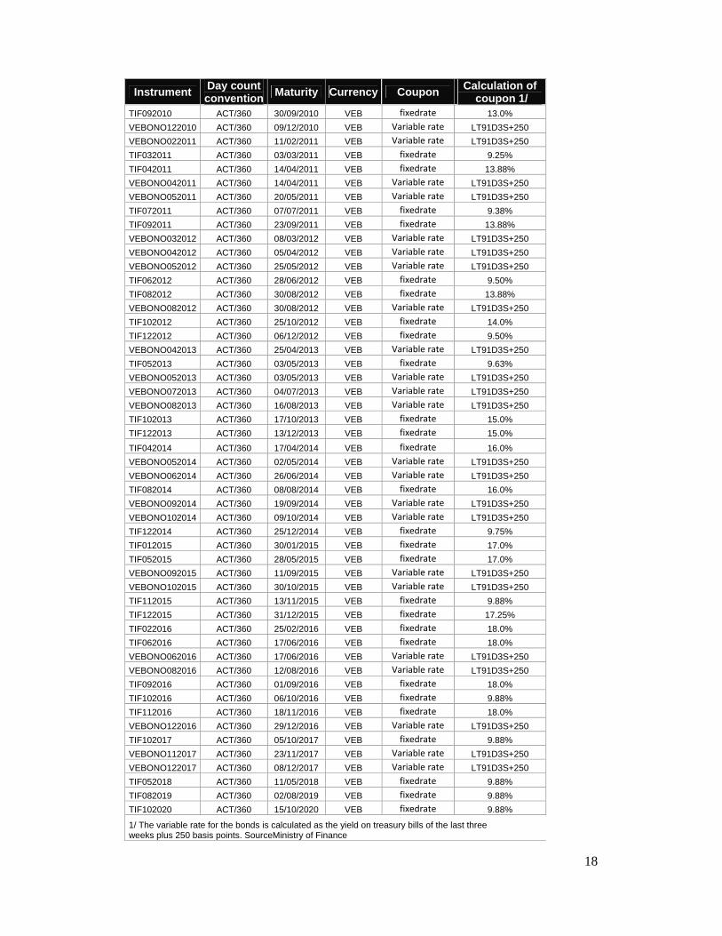
On the other hand, we use monthly data from April 2005 to December 20116 in external
market. In this market, debt securities are mainly fixed coupon instruments issued by
Venezuelan government and denominated in US$ dollars; which represents a portion of
its external public debt. Data selected includes a set of 14 bonds with a maturity horizon
around 30 years.
For both markets, information regarding debt instruments includes: clean prices, yields
to maturity, coupon rates, coupon payment dates and maturities. Such variables were
obtained from Reuters (external debt market), and Sistema de Custodia Electrónica de
Títulos -SICET (local debt market). All trading negotiations refer to secondary market
6Sample of each market differs since we consider as estimation requirement at least an amount of 10 bonds to estimate yield curve, and this conditions is fulfill for foreign debt market after 2005. We consider necessary, at least, 10 instruments since NS characterization requires a minimum set of 4 observations.
7
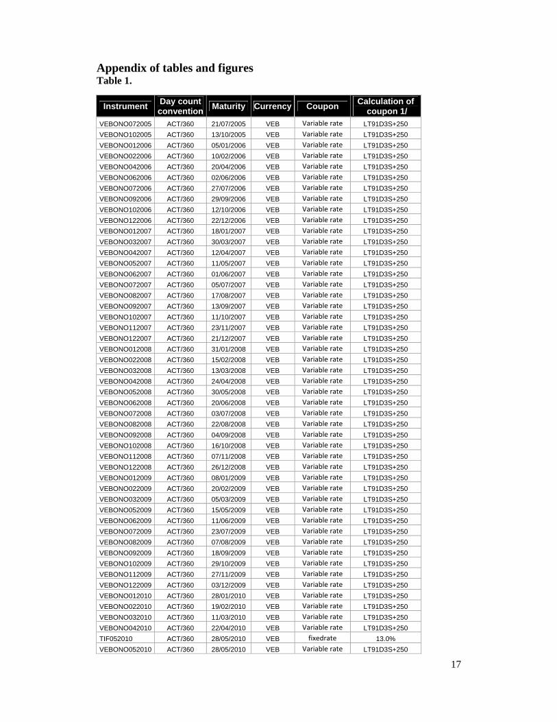
transactions. Table 1 and table 2 show main features of data used ranked by time to
maturity.
3. Estimation methodology In order to estimate equation (1) we apply a non-linear least-squares regression
technique to fit the cross- sectional set of monthly data for the markets evaluated7.
Fitting procedure is computed under an optimization problem (i.e. minimization of
squared errors between observed and estimated yield) with an initial set of parameters
for the coefficients to be estimated. The assumptions used to select the ranges of starting
values are the following: 0 represents yield of the bond with longest term to maturity
in the data sample; 1 is the difference of the yields between the longest and shortest
term to maturity; 2 is the associated to yields of bonds with medium-term to maturity
and is the average maturity of bonds in medium term. 0 and were constrained to be
positive as the model predicts.
Optimization mechanism requires error minimization yields, defined as the difference of
the equation (1) respect to historical observed yields. Even when optimization do not
minimize price errors, along the estimation procedure we compute, after each iteration,
cash flows related to every instrument and theoretical prices8 for the different
parameters of NS model. In this way, we simultaneously obtain the theoretical price
associated to the forward rate that minimizes yield errors.
To guarantee accuracy of the final results, different (increasing) numbers of replications
were considered through the algorithm of Gauss Newton. Once forward rates are
estimated under equation (1), we determine conditional variance according to equation
(2) for cross sectional dataset of two markets. In this fashion, we get conditional
volatility, for each instrument associated to a specific maturity. In short, this leads us to
7As alternative techniques, Maximum Likelihood Estimator (MLE) or Generalized Method of Moments (GMM) can be also applied 8
),(),(1
TtDCFTtPN
tNN
, where CF are the cash flows of the Nth bond and D (t,T) is the discount
function.
8
obtain volatility term structure. For comparative purposes, we reduce dimensionality of
conditional variance across the amount of bonds considered and maturities; using its
representative factors through principal components analysis (PCA). Finally, we
compare these factors representing volatility and parameters 0 , 1 , 2 with a group of
macroeconomic variables, to infer their possible interrelations and the reasons that
generate movements on yield curve and the volatility of term structure.
4. Empirical results 4.1 TSIR analysis and parameters from NS This section analyzes the term structure in terms of the shapes of the yield curve y and
its variance, providing conjectures of their different shapes exhibited, depending on the
market in which they were traded and issued. For the whole sample (both markets) we
find three types of yield curve: upward sloping, downward sloping, and humped yield
curves9. Description of different periods related to these patterns is summarized in the
following paragraphs of this section.
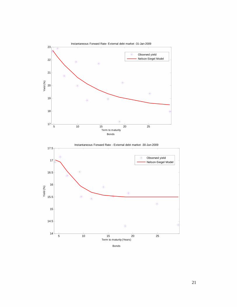
For external debt, during May 2005- September 2008, a positive or normal pattern was
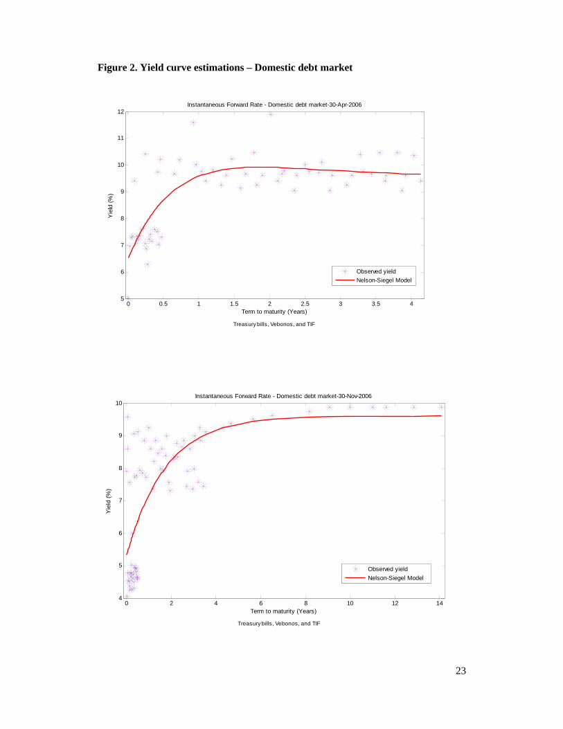
exhibited by yield curve. Domestic debt market replicated this fashion from July 2005
to June 2008. Presence of “positive” yield curves would corroborate expectation
hypothesis theory, that claims that forward rates increase along maturities and those are
always higher than future spot rates. However, one can argue that bond holders are so
risk adverse, that they invest in short term maturities, and the only way we able to hold
long term bonds if they get a risk premium in exchange to face higher levels of
exposure10. Additionally and using the theory of term premium (captured by the slope
of term structure, i.e. spread of long term and short term interest rates) and its positive
relation with economic growth and inflation rate (Fama 1990, Miskin 1990a, and
Estrella and Mishkin, 1996).So, upward sloping yield curve would be reflecting
Venezuelan bond holders’ expectations about economic growth in the future and
inflationary pressures. Indeed, empirically speaking, the period mentioned for positives
yield curve coincides with GDP annual growth rates above 5% accompanied with 9Even when extended version of Nelson- Sigel model ( Svensson, 1994) was formulated to captured the “humped” yield curves, the application of the original Nelson Siegel characterization was able to reproduce them. 10 This theory is called liquidity preference; see Hicks (1946) for more details.
9
variations of consumer prices index (CPI) around 20%. It seems that there exist
elements to infer that such economic performance could have been extracted from the
information imbedded in yield curve.
However, in the period October 2008 - July 2009, foreign yield curve reverted its
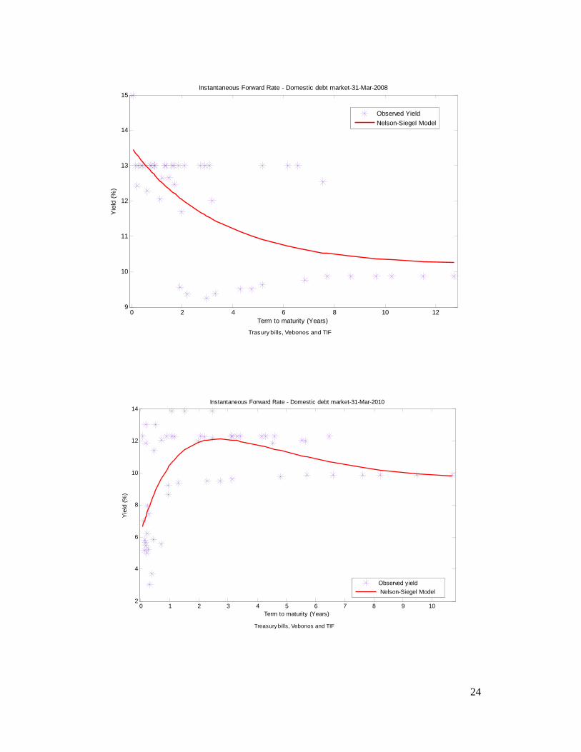
positive sloping pattern into an inverted one. In the domestic debt market this type of
curves is replicated during February 2008 to August 2009. Theoretically a downward
sloping yield curve occurs when short-term yields exceeds long term rates. These curves
are commonly used as leading indicator of future recessions. In fact, it does not seem
fortuitous that these periods of time occur during the fall of oil prices (May 2008) and
the global financial collapse (September 2008). Even when Venezuelan economic
contraction effectively occurred during the first term of 2009, it is possible to argue that
traders anticipated the negative impact that contraction of oil market would be
generating on real sector due to dependence on oil exports.
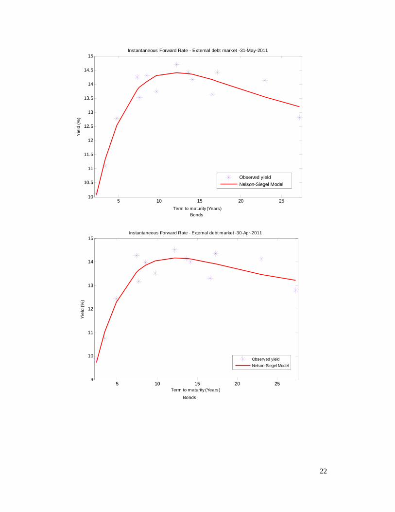
On the other hand, last type of pattern showed by the yield curve was the “humped”
shaped. A key issue is that this pattern appears mainly for the shortest maturities, to
then decrease from mid-term to long term maturities. For external debt market, such
“humped” behavior is presented in two periods: November 2009 - February 2010, and
August 2010 - January 2011. This is because long term bonds (30 years) in this market
were more liquid and had stable returns over time than short term bonds, which reported
the highest variations of their yields.
For domestic debt market, humped yield curves appeared from January 2009 to the end
of the sample. For this market, humped pattern was associated to maturity of four years;
where the hump achieved its maximum value to start to decline for the rest of
maturities. Such feature is mainly attributable to the borrowing strategy implemented by
the National Public Credit Office during 2009-2010, in where financial instruments
were issued around 4 years of maturity.
Figure 1 and figure 2 shows all the patterns described in this section.
10
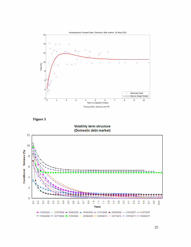
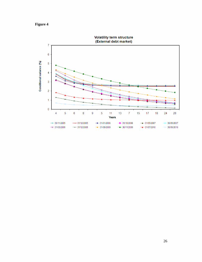
4.2 Volatility term structure
The second moment of the TSIR was computed using EGARCH (1,1) model. Results
reveal some similar characteristics regarding volatility term structure for both markets.
External market results’ along the whole sample indicates that bonds with maturity
inferior than 12 years are more volatile than long term bonds (16 – 30 years of term to
maturity). We emphasize the period October 2008 - July 2009, in which yield curves
were downward sloping, the entire structure of observed yields increased abruptly (
from 14% to 19% ) across all maturity spectrum, especially more than proportional for
those short term debt securities (figure 3). This effect modified the magnitudes of
conditional variance for all bonds outstanding. However, it was reverted in 2009, when
observed bond returns recovered their initial trend (10% -13 % in average).
On the other hand, conditional variance, for short term bonds (less than 3 years) issued
on domestic market are superior that variance of long term bonds. Indeed, this feature is
replicated along the sample as well (figure 4). As shown in external debt market, during
2008 and the beginning of 2009, the level of conditional variance rises across
maturities. For both markets, as argued in previous section, the fall in oil prices could
explain the unexpected fluctuations in bond returns. Nevertheless, domestic
instruments, historical yields did not return to their previous levels as external debt
market did.
So, it seems that independently the type of market considered, in terms of second
moment of TSIR, debt securities instruments with short term to maturity have a high
conditional variance. However, when both markets are compared between them, since
maturity horizons differ, if we abstract of negotiation conditions, short term bonds from
foreign market would be equivalent to long term bonds of domestic market. Under this
scenario and using the basis of financial foundations; long term bonds tend to show
stable returns across time. These debt instruments display a VTS superior to the
expected for the maturity associated.
11
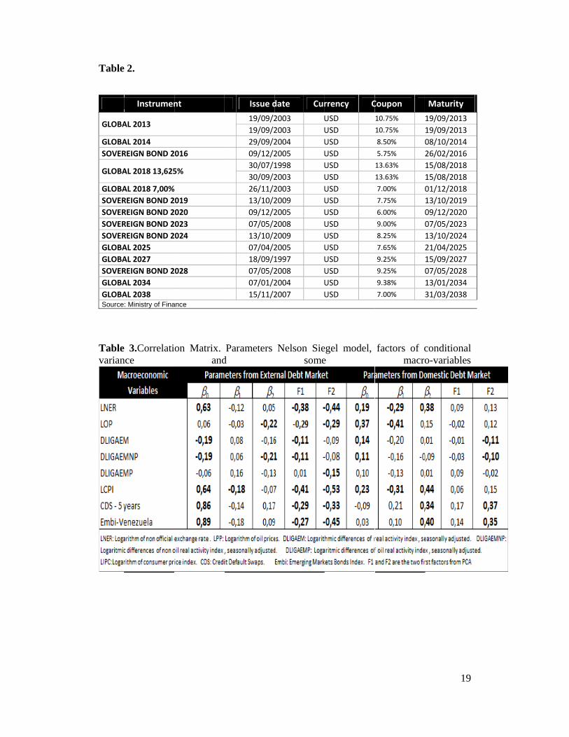
4.3 Parameters from NS, principal components analysis (PCA) of VTS and some
macro variables
Previous section has analysed, how the shapes and movements of yield curve are
interrelated with VTS, but the underlying set of possible variables that make changes on
both financial indicators are still missing in the analysis. In this context arises the
typical question regarding macroeconomic factors driven their variations. Literature has
tried to generate a macroeconomic interpretation of yield curve (Litterman and
Scheinkman 1991, Bliss 1997, Wu 2001,Dielbod-Li 2005, Pérignon and Villa 2006).
The last purpose of the research is to establish different signals respect the variables that
promote variations on these financial indicators. We do not pretend to statically
determine a model to reproduce such movements, instead we just conjecture the
potential relations among a selection of macroeconomic variables, parameters of NS
model, and conditional variance of forward rates. In order to do so, as mentioned in
section 3, dimensionality of conditional variance must be reduced. So, we shrink the
range of maturities and number of bonds for each type of market using PCA. Previous
researches, Novales and Benito (2007) and Diaz et al. (2010), apply same analysis for
Spanish debt market. For Venezuelan case, and to our knowledge, this is the first
approximation applied to debt market. Using PCA, we select the two first factors (F1,
F2) for each market that account around 98 % of accumulative variance for both
markets, and they represent the volatility of instruments of short and medium term.
Using these factors, we compute a correlation matrix (Table 3), taking into account
parameters estimated from NS ( 210 ,, ), and some macroeconomics and financial
variables. Financial variables selected are: Credit Default Swap (CDS) and Emerging
Market Bond Index (EMBI). Both variables refer to investors’ expectations about
economic performance and government financial health. Economic variables selected
and showed statistically significant relations are: non official exchange rate (NER), oil
prices (OP), and indexes for: monthly real activity (IGAEM), monthly real oil activity
(IGAEMP), monthly real non - oil activity (IGAEMNP), and the consumer price index
(CPI). Variables coming from real sector are expressed in logarithmic differences, while
variables associated to prices (exchange rate, oil prices, and CPI) are included in
logarithmic levels.
12
Establishing the degree of lineal association, we find that long term component ( 0 ) of
foreign market is positively correlated with CDSand EMBI (89% and 86%
respectively). These variables are common referred as reflecting the implicit risk in the
conditions of debt market; it is possible conjecture that movements in the level of yield
curve could be mainly associated to changes in the market valuation of financial
conditions for Venezuelan government. Besides, this parameter for foreign debt market
is moderate correlated with positive changes in non- official exchange rate (63%) and
CPI (64%). These lineal relationships are remained in direction but they decrease in
magnitude for local debt market (19% y 23% respectively). For the Venezuelan
economy and due to the existence of exchange control rate, depreciations that occur in
non- official market are directly translated into the returns of the instruments negotiated
in debt market. The link of 0 with changes in CPI has been previously pointed out by
Wu (2003). According to this author and since this unobservable parameter refers to the
long term expectations, movements in expected inflation rate would finally alter real
long term interest rates and influence the level of yield curve. In few words, as a result
of high inflation expectations, agents anticipate the rise in interest with the intention of
mitigate the effects of future inflation pressures.
Besides, its links with price variables, there exists lightly relationship between 0 and
the real sector. Magnitudes of this relationship are partially similar for both markets;
however, sign of direction is the opposite. In foreign market, long term component and
productive sector are related in a negative way. Intuition behind this is the following:
Since the level can be considered as a proxy of credit risk, adverse economic conditions
will exacerbate expectations of a poor financial performance of government sector.
Nevertheless, in internal debt market the association is essentially positive; clamming
that under economic growth scenarios returns of instruments increase, shifting the level
of yield curve as a whole.
Even, when oil prices do not show high correlation with foreign long term parameter, as
we can expect, it does for domestic market. A boost in oil prices would tend, ceteris
paribus, to shift the level of yield curve as the rest of real variables do.
On the other hand and for both markets, the short term component of yield curve ( 1 ) is
negative affected by inflationary pressures. As mention in section 1, this last parameter
13
is well known as the slope of yield curve, which means that periods with high inflation
rates would shift down slope of term structure of interest rates. Therefore, not only
positive variations in prices contract slope of yield curve, depreciations of non official
exchange rate, and the increment in oil prices, cause the same outcome in the local debt
market. In short, changes of price variables impact slope of yield curve for the
Venezuelan debt market.
Foreign medium term component ( 2 ), that measures curvature and steepness of yield
curve, is negative related with oil prices (22%), i.e. during episodes of drop in oil prices
humped shapes are more likely to occur. This could explain the presence of this
characteristic in external market at the end of 2008, when oil prices abruptly declined
after a period of expansion. In the case of domestic, external variables (non- official
exchange rate, CDS and EMBI) and prices could be driven changes in the curvature of
yield curve, and they would reproduce a steeper yield curve as well. Besides, we figure
out that humps, in the internal market, are more likely to take place for short term
maturities while in the external market such humps are linked to medium term
instruments.
Regarding the factors (F1 and F2) extracted from conditional variance, the factor of
short term volatility (F1) of foreign market, is negative correlated with all the variables
in table 3. However, the strongest correlation comes from non- official exchange rate
and CPI. Relevant is the small relationship between this factor and real sector variables,
which implies that under economic expansions volatility of foreign short term debt
instruments is reduced, due to expectations of Venezuelan bond holders improves and
the speed at which instruments are traded with arbitrage opportunities purposes
declines. These relationships, excluding real variables, remain for the factor of medium
term volatility (F2) of foreign debt market. Although, F2 for domestic market,
reproduce correlations of similar magnitude than factor of short term volatility of
external market for real variables; contractions in real production volatility of medium
term bonds increases. Therefore, this factor shifts its value as a result of a greater credit
risk.
14
Different from the results found by Diaz et al. (2010), in which factors of conditional
variance are equivalent to the unobservable components of NS model, for the
Venezuelan case, these relationships are negligible.
5. Concluding remarks
The versatility of term structure and its ability to connecting the puzzling associations
between macroeconomic variables and financial systems is one of the arguments to
argue why this indicator is continuously used by analyst and policy makers. After
consequences of subprime crises, financial world found another way of extracting
information regarding investors’ expectations, through the volatility of the yield curve.
When we analyze Venezuelan debt market comparatively is relevant the way how the
patterns exhibited by yield curve are shared for external and domestic debt instruments,
during analogous period of time. Even when is true, that negotiation conditions of debt
instruments differ across market, investors expectations’ of their bond holders seem to
follow same tendency and be caused by the same factors. Remaining question is
whether both markets simultaneously share invertors.
Alternatively, at the beginning of the sample the vast majority of the estimations
displayed an upward sloping fashion coinciding with periods of economic expansion.
However, during the financial distress, drop in oil prices and contractions of Venezuelan
economic, representatives yield curve exhibited a downward sloping pattern while
humped yield curve characterized both market at the end of the sample used. These
movements of yield curve encourage the continuous conjectures of relationships
between real sector of the economy and shapes of yield curve. In this context, it does
not seem random that long term component of NS is strongly connected to the
economic fundamentals and variables related to financial risk (CDS and EMBI).
Besides, a shift down of slope of yield curve could be linked to depreciations, inflation
and oil price expansions, while steepness of yield curve is mainly driven by changes in
prices and external sector variables. It means that factors that alter slope of yield curve
are associated to price variables.
15
In addition, debt instruments of short term are more volatile than long term bonds.
Nevertheless, short term bonds from external debt market have a higher conditional
variance than their equivalent instruments, in terms of maturity, from domestic market.
In this sense, expansions of real sector would reduce volatility of debt securities in both
markets, i.e. under better economic performance, investor’s expectation improves and
the fluctuations of instruments traded decreases.
Finally, the naïve relationships discussed here are far away from being conclusive.
Evidently, there still remains an open questing that must to be dealt in further research
about incorporating in an appropriate statistical and mathematical representation,
macroeconomic elements for the estimation of yield curve and VTS.
References Black, F and Scholes, M (1973): “The Pricing of Options and Corporate Liabilities. Journal of Political Economy, 72, pp. 637-659. Bollerslev, T.(1986). Generalized autoregressive conditional heteroskedasticity.Journal of Econometrics, 31, pp. 307-327. Bollerslev T, Chou R, Kroner, K. (1992). ARCH modelling in finance.Journal of Econometrics, 52, pp. 5-59. Benito, S. and Novales, A. (2005).A factor analysis of volatility across the term structure: the Spanish case, mimeo. Cox, J., Ingersoll, J and Ross, S (1985): An Intertemporal General Equilibrium Model of Assets Prices. Econometrica, 53, pp. 363-384. Chirinos, A. and Moreno, M. (2010). Estimation of the Term Structure of Interest Rates: The Venezuelan Case. Central Bank of Venezuela, Working paper series N° 119 (forthcoming) Culbertson, J.M. (1957). The Term Structure of Interest Rates. Quarterly Journal of Economics, 71, 485-517. Diaz, J. and Ibáñez, A (2006): Estimation with Applications of Two Factors Affine Term Structure for Mexico, 1995-2004, mimeo. Díaz A, Jareño F, Navarro E. (2010b). A Principal Component Analysis of the Spanish Volatility Term Structure.International Research Journal of Finance and Economics, 49, pp. 150-155.
16
Díaz A, Jareño F, Navarro E. (2011a). Term Structure of Volatilities and Yield Curve Estimation Methodology.Quantitative Finance, 11 (4), pp. 573-586. Diebold, F. and Li, C. (2005).Forecasting the term structure of government bond yields.Journal of Econometrics, 130, pp. 337-364 Engle, R. (1982). Autoregressive conditional heteroskedasticity with estimates of the variance of U.K. inflation.Econometrica, 50, 987–1008 Estrella, A. and Mishkin, F. (1996): Predicting U.S. recessions: Financial variables as leading indicators, Research Paper 9690. Federal Reserve Bank of New York. Fisher, I. (1930) Theory of Interest, New York, Macmillan. Jareño, F. and M. Tolentino (2011). The US volatility term structure: A principal component analysis. Journal of Business Management, 6(2), pp. 615-626. Kozicki, S (1997): Predicting real growth and inflation with the yield spread. Economic Review, Federal Reserve Bank of Kansas City, issue Q IV, pages 39-57. Litterman. R. and Scheinkman, J.(1991). Common Factors Affecting Bond Returns.Journal of Fixed Income, 1(1), pp. 54-61 Maita, M (2011). Estimación de una curva de rendimientos para los bonos de la deuda pública interna en Venezuela, mimeo. Modigliani, M and R. Sutch (1966).Innovations in Interest Rate Policy.American Economic Review, 56, 178-197. Nelson, C. R. and A. F. Siegel (1987). Parsimonious modelling of yield curves, Journal of Business, 60, 473-89. Perignon, C. and Villa, C. (2006).Sources of time variation in the covariance matrix of interest rates.Journal of Business, 79(3), 1536–1549 Svensson, L. (1994): Estimating and interpreting forward interest rates: Sweden 1992-1994, CEPR Discussion Paper Series, No 1051, October (also: NBER Working Paper Series, No 4871). Wu, Tao. (2003). What makes the yield curve move?. FRBSF Financial Letter, 15, June 6.
17
Appendix of tables and figures Table 1.
Instrument Day count convention
Maturity Currency Coupon Calculation of
coupon 1/
VEBONO072005 ACT/360 21/07/2005 VEB Variable rate LT91D3S+250
VEBONO102005 ACT/360 13/10/2005 VEB Variable rate LT91D3S+250
VEBONO012006 ACT/360 05/01/2006 VEB Variable rate LT91D3S+250
VEBONO022006 ACT/360 10/02/2006 VEB Variable rate LT91D3S+250
VEBONO042006 ACT/360 20/04/2006 VEB Variable rate LT91D3S+250
VEBONO062006 ACT/360 02/06/2006 VEB Variable rate LT91D3S+250
VEBONO072006 ACT/360 27/07/2006 VEB Variable rate LT91D3S+250
VEBONO092006 ACT/360 29/09/2006 VEB Variable rate LT91D3S+250
VEBONO102006 ACT/360 12/10/2006 VEB Variable rate LT91D3S+250
VEBONO122006 ACT/360 22/12/2006 VEB Variable rate LT91D3S+250
VEBONO012007 ACT/360 18/01/2007 VEB Variable rate LT91D3S+250
VEBONO032007 ACT/360 30/03/2007 VEB Variable rate LT91D3S+250
VEBONO042007 ACT/360 12/04/2007 VEB Variable rate LT91D3S+250
VEBONO052007 ACT/360 11/05/2007 VEB Variable rate LT91D3S+250
VEBONO062007 ACT/360 01/06/2007 VEB Variable rate LT91D3S+250
VEBONO072007 ACT/360 05/07/2007 VEB Variable rate LT91D3S+250
VEBONO082007 ACT/360 17/08/2007 VEB Variable rate LT91D3S+250
VEBONO092007 ACT/360 13/09/2007 VEB Variable rate LT91D3S+250
VEBONO102007 ACT/360 11/10/2007 VEB Variable rate LT91D3S+250
VEBONO112007 ACT/360 23/11/2007 VEB Variable rate LT91D3S+250
VEBONO122007 ACT/360 21/12/2007 VEB Variable rate LT91D3S+250
VEBONO012008 ACT/360 31/01/2008 VEB Variable rate LT91D3S+250
VEBONO022008 ACT/360 15/02/2008 VEB Variable rate LT91D3S+250
VEBONO032008 ACT/360 13/03/2008 VEB Variable rate LT91D3S+250
VEBONO042008 ACT/360 24/04/2008 VEB Variable rate LT91D3S+250
VEBONO052008 ACT/360 30/05/2008 VEB Variable rate LT91D3S+250
VEBONO062008 ACT/360 20/06/2008 VEB Variable rate LT91D3S+250
VEBONO072008 ACT/360 03/07/2008 VEB Variable rate LT91D3S+250
VEBONO082008 ACT/360 22/08/2008 VEB Variable rate LT91D3S+250
VEBONO092008 ACT/360 04/09/2008 VEB Variable rate LT91D3S+250
VEBONO102008 ACT/360 16/10/2008 VEB Variable rate LT91D3S+250
VEBONO112008 ACT/360 07/11/2008 VEB Variable rate LT91D3S+250
VEBONO122008 ACT/360 26/12/2008 VEB Variable rate LT91D3S+250
VEBONO012009 ACT/360 08/01/2009 VEB Variable rate LT91D3S+250
VEBONO022009 ACT/360 20/02/2009 VEB Variable rate LT91D3S+250
VEBONO032009 ACT/360 05/03/2009 VEB Variable rate LT91D3S+250
VEBONO052009 ACT/360 15/05/2009 VEB Variable rate LT91D3S+250
VEBONO062009 ACT/360 11/06/2009 VEB Variable rate LT91D3S+250
VEBONO072009 ACT/360 23/07/2009 VEB Variable rate LT91D3S+250
VEBONO082009 ACT/360 07/08/2009 VEB Variable rate LT91D3S+250
VEBONO092009 ACT/360 18/09/2009 VEB Variable rate LT91D3S+250
VEBONO102009 ACT/360 29/10/2009 VEB Variable rate LT91D3S+250
VEBONO112009 ACT/360 27/11/2009 VEB Variable rate LT91D3S+250
VEBONO122009 ACT/360 03/12/2009 VEB Variable rate LT91D3S+250
VEBONO012010 ACT/360 28/01/2010 VEB Variable rate LT91D3S+250
VEBONO022010 ACT/360 19/02/2010 VEB Variable rate LT91D3S+250
VEBONO032010 ACT/360 11/03/2010 VEB Variable rate LT91D3S+250
VEBONO042010 ACT/360 22/04/2010 VEB Variable rate LT91D3S+250
TIF052010 ACT/360 28/05/2010 VEB fixedrate 13.0%
VEBONO052010 ACT/360 28/05/2010 VEB Variable rate LT91D3S+250
18
Instrument Day count convention
Maturity Currency Coupon Calculation of
coupon 1/ TIF092010 ACT/360 30/09/2010 VEB fixedrate 13.0%
VEBONO122010 ACT/360 09/12/2010 VEB Variable rate LT91D3S+250
VEBONO022011 ACT/360 11/02/2011 VEB Variable rate LT91D3S+250
TIF032011 ACT/360 03/03/2011 VEB fixedrate 9.25%
TIF042011 ACT/360 14/04/2011 VEB fixedrate 13.88%
VEBONO042011 ACT/360 14/04/2011 VEB Variable rate LT91D3S+250
VEBONO052011 ACT/360 20/05/2011 VEB Variable rate LT91D3S+250
TIF072011 ACT/360 07/07/2011 VEB fixedrate 9.38%
TIF092011 ACT/360 23/09/2011 VEB fixedrate 13.88%
VEBONO032012 ACT/360 08/03/2012 VEB Variable rate LT91D3S+250
VEBONO042012 ACT/360 05/04/2012 VEB Variable rate LT91D3S+250
VEBONO052012 ACT/360 25/05/2012 VEB Variable rate LT91D3S+250
TIF062012 ACT/360 28/06/2012 VEB fixedrate 9.50%
TIF082012 ACT/360 30/08/2012 VEB fixedrate 13.88%
VEBONO082012 ACT/360 30/08/2012 VEB Variable rate LT91D3S+250
TIF102012 ACT/360 25/10/2012 VEB fixedrate 14.0%
TIF122012 ACT/360 06/12/2012 VEB fixedrate 9.50%
VEBONO042013 ACT/360 25/04/2013 VEB Variable rate LT91D3S+250
TIF052013 ACT/360 03/05/2013 VEB fixedrate 9.63%
VEBONO052013 ACT/360 03/05/2013 VEB Variable rate LT91D3S+250
VEBONO072013 ACT/360 04/07/2013 VEB Variable rate LT91D3S+250
VEBONO082013 ACT/360 16/08/2013 VEB Variable rate LT91D3S+250
TIF102013 ACT/360 17/10/2013 VEB fixedrate 15.0%
TIF122013 ACT/360 13/12/2013 VEB fixedrate 15.0%
TIF042014 ACT/360 17/04/2014 VEB fixedrate 16.0%
VEBONO052014 ACT/360 02/05/2014 VEB Variable rate LT91D3S+250
VEBONO062014 ACT/360 26/06/2014 VEB Variable rate LT91D3S+250
TIF082014 ACT/360 08/08/2014 VEB fixedrate 16.0%
VEBONO092014 ACT/360 19/09/2014 VEB Variable rate LT91D3S+250
VEBONO102014 ACT/360 09/10/2014 VEB Variable rate LT91D3S+250
TIF122014 ACT/360 25/12/2014 VEB fixedrate 9.75%
TIF012015 ACT/360 30/01/2015 VEB fixedrate 17.0%
TIF052015 ACT/360 28/05/2015 VEB fixedrate 17.0%
VEBONO092015 ACT/360 11/09/2015 VEB Variable rate LT91D3S+250
VEBONO102015 ACT/360 30/10/2015 VEB Variable rate LT91D3S+250
TIF112015 ACT/360 13/11/2015 VEB fixedrate 9.88%
TIF122015 ACT/360 31/12/2015 VEB fixedrate 17.25%
TIF022016 ACT/360 25/02/2016 VEB fixedrate 18.0%
TIF062016 ACT/360 17/06/2016 VEB fixedrate 18.0%
VEBONO062016 ACT/360 17/06/2016 VEB Variable rate LT91D3S+250
VEBONO082016 ACT/360 12/08/2016 VEB Variable rate LT91D3S+250
TIF092016 ACT/360 01/09/2016 VEB fixedrate 18.0%
TIF102016 ACT/360 06/10/2016 VEB fixedrate 9.88%
TIF112016 ACT/360 18/11/2016 VEB fixedrate 18.0%
VEBONO122016 ACT/360 29/12/2016 VEB Variable rate LT91D3S+250
TIF102017 ACT/360 05/10/2017 VEB fixedrate 9.88%
VEBONO112017 ACT/360 23/11/2017 VEB Variable rate LT91D3S+250
VEBONO122017 ACT/360 08/12/2017 VEB Variable rate LT91D3S+250
TIF052018 ACT/360 11/05/2018 VEB fixedrate 9.88%
TIF082019 ACT/360 02/08/2019 VEB fixedrate 9.88%
TIF102020 ACT/360 15/10/2020 VEB fixedrate 9.88%
1/ The variable rate for the bonds is calculated as the yield on treasury bills of the last three weeks plus 250 basis points. SourceMinistry of Finance
Table
GLOBA
GLOBA
SOVER
GLOBA
GLOBA
SOVER
SOVER
SOVER
SOVER
GLOBA
GLOBA
SOVER
GLOBA
GLOBASource
Table varian
2.
Instrumen
AL 2013
AL 2014
REIGN BOND 2
AL 2018 13,625
AL 2018 7,00%
REIGN BOND 2
REIGN BOND 2
REIGN BOND 2
REIGN BOND 2
AL 2025
AL 2027
REIGN BOND 2
AL 2034
AL 2038 : Ministry of Fina
3.Correlatince
nt
016
5%
019
020
023
024
028
ance
on Matrix. and
Issue d
19/09/2
19/09/2
29/09/2
09/12/2
30/07/1
30/09/2
26/11/2
13/10/2
09/12/2
07/05/2
13/10/2
07/04/2
18/09/1
07/05/2
07/01/2
15/11/2
Parameters d
date Cur
2003 U
2003 U
2004 U
2005 U
1998 U
2003 U
2003 U
2009 U
2005 U
2008 U
2009 U
2005 U
1997 U
2008 U
2004 U
2007 U
Nelson Siesome
rrency C
USD
USD
USD
USD
USD
USD
USD
USD
USD
USD
USD
USD
USD
USD
USD
USD
egel model, e
Coupon
10.75%
10.75%
8.50%
5.75%
13.63%
13.63%
7.00%
7.75%
6.00%
9.00%
8.25%
7.65%
9.25%
9.25%
9.38%
7.00%
factors of cmacro
19
Maturity
19/09/2013
19/09/2013
08/10/2014
26/02/2016
15/08/2018
15/08/2018
01/12/2018
13/10/2019
09/12/2020
07/05/2023
13/10/2024
21/04/2025
15/09/2027
07/05/2028
13/01/2034
31/03/2038
conditional o-variables
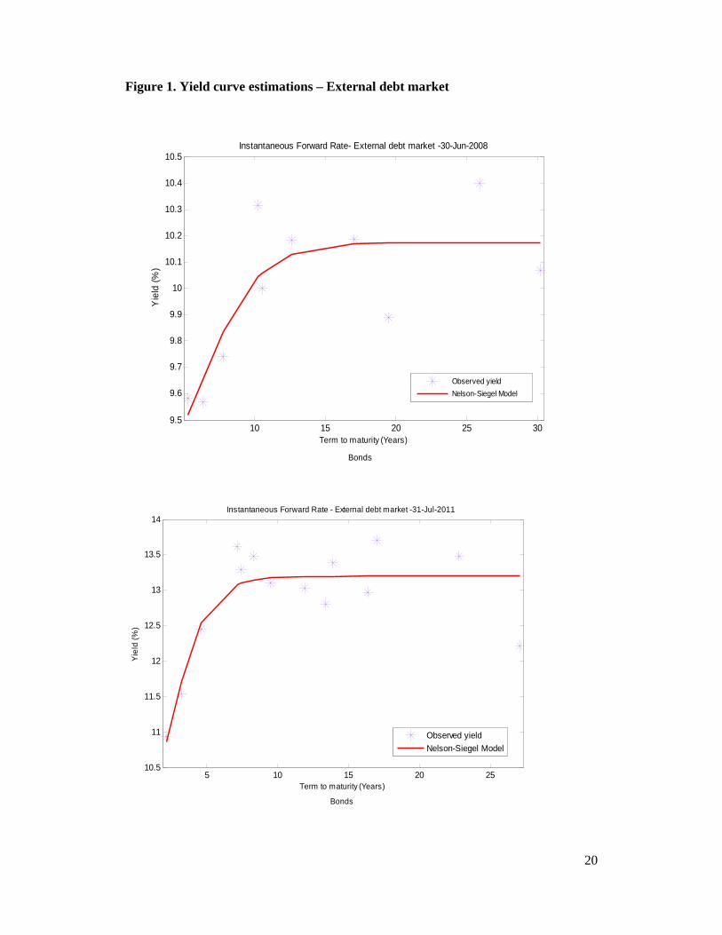
20
10 15 20 25 309.5
9.6
9.7
9.8
9.9
10
10.1
10.2
10.3
10.4
10.5
Term to maturity (Years)
Yie
ld (
%)
Instantaneous Forward Rate- External debt market -30-Jun-2008
Observed yield
Nelson-Siegel Model
Bonds
Figure 1. Yield curve estimations – External debt market
5 10 15 20 2510.5
11
11.5
12
12.5
13
13.5
14
Term to maturity (Years)
Yie
ld (
%)
Instantaneous Forward Rate - External debt market -31-Jul-2011
Observed yield
Nelson-Siegel Model
Bonds
21
5 10 15 20 2517
18
19
20
21
22
23
Term to maturity
Yie
ld (
%)
Instantaneous Forward Rate- External debt market -31-Jan-2009
Observed yield
Nelson-Siegel Model
Bonds
5 10 15 20 2514
14.5
15
15.5
16
16.5
17
17.5
Term to maturity (Years)
Yie
ld (
%)
Instantaneous Forward Rate - External debt market -30-Jun-2009
Observed yield
Nelson-Siegel Model
Bonds
22
5 10 15 20 2510
10.5
11
11.5
12
12.5
13
13.5
14
14.5
15
Term to maturity (Years)
Yie
ld (
%)
Instantaneous Forward Rate - External debt market -31-May-2011
Observed yield
Nelson-Siegel Model
Bonds
5 10 15 20 259
10
11
12
13
14
15
Term to maturity (Years)
Yie
ld (
%)
Instantaneous Forward Rate - External debt market -30-Apr-2011
Observed yield
Nelson-Siegel Model
Bonds
23
Figure 2. Yield curve estimations – Domestic debt market
0 0.5 1 1.5 2 2.5 3 3.5 45
6
7
8
9
10
11
12
Term to maturity (Years)
Yie
ld (
%)
Instantaneous Forward Rate - Domestic debt market-30-Apr-2006
Observed yield
Nelson-Siegel Model
Treasury bills, Vebonos, and TIF
0 2 4 6 8 10 12 144
5
6
7
8
9
10
Term to maturity (Years)
Yie
ld (
%)
Instantaneous Forward Rate - Domestic debt market-30-Nov-2006
Observed yield
Nelson-Siegel Model
Treasury bills, Vebonos, and TIF
24
0 2 4 6 8 10 129
10
11
12
13
14
15
Term to maturity (Years)
Yie
ld (
%)
Instantaneous Forward Rate - Domestic debt market-31-Mar-2008
Observed Yield
Nelson-Siegel Model
Trasury bills, Vebonos and TIF
0 1 2 3 4 5 6 7 8 9 102
4
6
8
10
12
14
Term to maturity (Years)
Yie
ld (
%)
Instantaneous Forward Rate - Domestic debt market-31-Mar-2010
Observed yield
Nelson-Siegel Model
Treasury bills, Vebonos and TIF
25
Figure 3
0 1 2 3 4 5 6 7 8 9 102
4
6
8
10
12
14
16
Term to maturity (Years)
Yie
ld (
%)
Instantaneous Forward Rate- Domestic debt market -31-May-2010
Observed yield
Nelson-Siegel Model
Treasury bills, Vebonos and TIF
26
Figure 4


![[Salomon Brothers] Understanding the Yield Curve, Part 5 - Convexity Bias and the Yield Curve](https://static.fdocuments.net/doc/165x107/577d26641a28ab4e1ea111d0/salomon-brothers-understanding-the-yield-curve-part-5-convexity-bias-and.jpg)