Upper bound shakedown analysis of elastic-plastic bounded ... · made of elastic plastic bounded...

Upper Bound Limit and Shakedown Analysis of Elastic-Plastic

Bounded Linearly Kinematic Hardening Structures

Von der Fakultät für Maschinenwesen

der Rheinisch-Westfälischen Technischen Hochschule Aachen

zur Erlangung des akademischen Grades eines

Doktors der Ingenieurwissenschaften

genehmigte Dissertation

vorgelegt von

Phu Tinh Pham

Berichter: Univ.-Prof. Dr.-Ing. Dieter Weichert

Prof. Dr.-Ing. (griech.) Christos D. Bisbos

Tag der mündlichen Prüfung: 28. Juli 2011

Diese Dissertation ist auf den Internetseiten der Hochulbibliothek online verfügbar.

http://www.rwth-aachen.de/

Dedication

To my parents

To Loan, Phượng, and Hồng Hà

Phạm Phú Tình

Acknowledgements

I would like to thank the Government of Vietnam, which granted me a scholarship

by the decision number: 7197/QĐ-BGDĐT, dated 04.12.2006 by Ministry of Education

and Training of Vietnam.

I would like to thank Aachen University of Applied Sciences, which supports me

financially and with good conditions for my research activities.

I will always be grateful to Prof. Dr.-Ing. Manfred Staat, Aachen University of

Applied Sciences, for not only giving me very clear orientation and guidance, but also the

best conditions and encouragement. The time of working on the Ph.D. thesis has been very

effective.

I would like to thank Prof. Dr.-Ing. Dieter Weichert, Rheinisch-Westfälische

Technische Hochschule Aachen (RWTH), for having kindly accepted my registration and

for his kind assistance and supervision.

I would like to thank Professor Dr.-Ing. Christos Bisbos, Aristotle University

Thessaloniki, Greece, for having kindly accepted to review this thesis.

I would like to thank Dr.-Ing. Vũ Đức Khôi and Dr.-Ing. Trần Thanh Ngọc for their

kind help and discussions.

I would like to say thank you to the open source software Code_Aster, which is the

solver of the problem.

Jülich, Germany, 2011

Phạm Phú Tình



The lower pictures have been illustrated by Phạm Phú Tình, dual to the upper pictures, copyright by Bill Waterson.

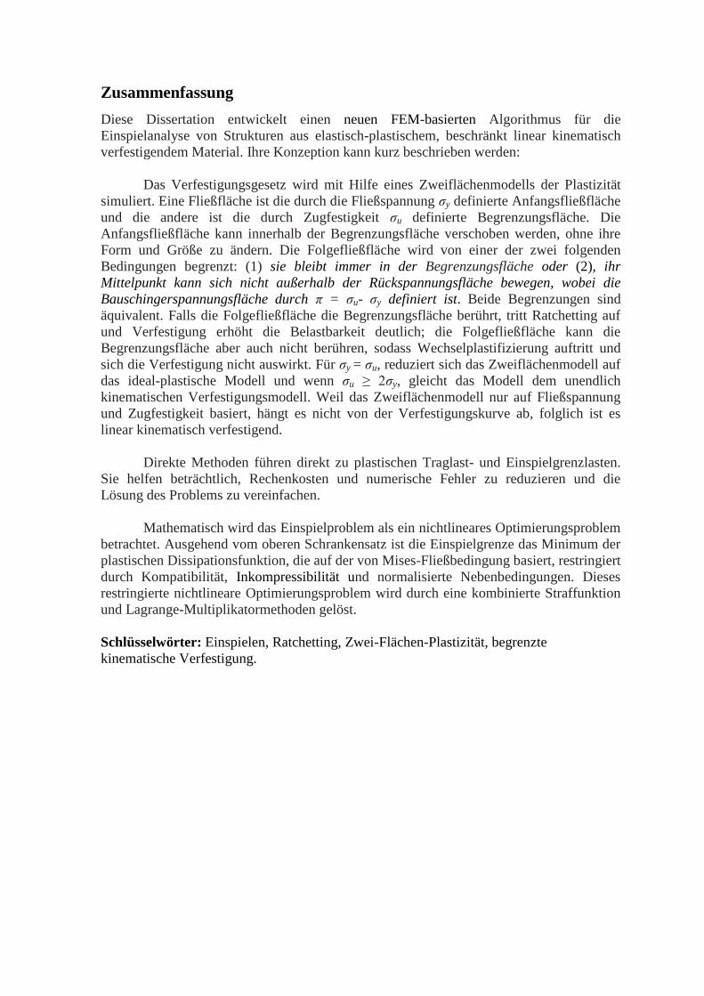
Abstract

This thesis develops a new FEM based algorithm for shakedown analysis of structures

made of elastic plastic bounded linearly kinematic hardening material. Its concept can be

briefly described as:

Hardening law is simulated using a two-surface plastic model. One yield surface is

the initial surface, defined by yield stress y , and the other one is the bounding surface,

defined by ultimate strength u . The initial surface can translate inside the bounding

surface without changing its shape and size. The subsequent yield surface is bounded by

one of the two following conditions: (1) it always stays inside the bounding surface, or (2)

its centre cannot move outside the back-stress surface, where the back-stress surface is

defined by u y . Both ways of bounding are equivalent. The subsequent yield

surface may touch the bounding surface, it means ratchetting occurs and benefit of

hardening is quite clear, or it may not touch the bounding surface, it means alternating

occurs, and there is no effect of hardening. If y u , the two-surface model becomes

elastic perfectly plastic model, and if 2u y , the model becomes unbounded kinematic

hardening model. Since the two-surface model bases only on yield stress and ultimate

strength, so it does not depend on the hardening curve, consequently it is linear kinematic

hardening.

Direct methods lead to plastic limit and shakedown bounds directly. They help to

reduce considerably computing costs and numerical errors, and make the solution simpler.

Mathematically, the shakedown problem is considered as a nonlinear programming

problem. Starting from upper bound theorem, shakedown bound is the minimum of the

plastic dissipation function, which is based on von Mises yield criterion, subjected to

compatibility, incompressibility and normalized constraints. This constraint nonlinear

optimization problem is solved by combined penalty function and Lagrange multiplier

methods.

Key words: shakedown, ratchetting, two-surface plasticity, bounded kinematic hardening.

Zusammenfassung

Diese Dissertation entwickelt einen neuen FEM-basierten Algorithmus für die

Einspielanalyse von Strukturen aus elastisch-plastischem, beschränkt linear kinematisch

verfestigendem Material. Ihre Konzeption kann kurz beschrieben werden:

Das Verfestigungsgesetz wird mit Hilfe eines Zweiflächenmodells der Plastizität

simuliert. Eine Fließfläche ist die durch die Fließspannung σy definierte Anfangsfließfläche

und die andere ist die durch Zugfestigkeit σu definierte Begrenzungsfläche. Die

Anfangsfließfläche kann innerhalb der Begrenzungsfläche verschoben werden, ohne ihre

Form und Größe zu ändern. Die Folgefließfläche wird von einer der zwei folgenden

Bedingungen begrenzt: (1) sie bleibt immer in der Begrenzungsfläche oder (2), ihr

Mittelpunkt kann sich nicht außerhalb der Rückspannungsfläche bewegen, wobei die

Bauschingerspannungsfläche durch π = σu- σy definiert ist. Beide Begrenzungen sind

äquivalent. Falls die Folgefließfläche die Begrenzungsfläche berührt, tritt Ratchetting auf

und Verfestigung erhöht die Belastbarkeit deutlich; die Folgefließfläche kann die

Begrenzungsfläche aber auch nicht berühren, sodass Wechselplastifizierung auftritt und

sich die Verfestigung nicht auswirkt. Für σy = σu, reduziert sich das Zweiflächenmodell auf

das ideal-plastische Modell und wenn σu ≥ 2σy, gleicht das Modell dem unendlich

kinematischen Verfestigungsmodell. Weil das Zweiflächenmodell nur auf Fließspannung

und Zugfestigkeit basiert, hängt es nicht von der Verfestigungskurve ab, folglich ist es

linear kinematisch verfestigend.

Direkte Methoden führen direkt zu plastischen Traglast- und Einspielgrenzlasten.

Sie helfen beträchtlich, Rechenkosten und numerische Fehler zu reduzieren und die

Lösung des Problems zu vereinfachen.

Mathematisch wird das Einspielproblem als ein nichtlineares Optimierungsproblem

betrachtet. Ausgehend vom oberen Schrankensatz ist die Einspielgrenze das Minimum der

plastischen Dissipationsfunktion, die auf der von Mises-Fließbedingung basiert, restringiert

durch Kompatibilität, Inkompressibilität und normalisierte Nebenbedingungen. Dieses

restringierte nichtlineare Optimierungsproblem wird durch eine kombinierte Straffunktion

und Lagrange-Multiplikatormethoden gelöst.

Schlüsselwörter: Einspielen, Ratchetting, Zwei-Flächen-Plastizität, begrenzte

kinematische Verfestigung.

i

Contents

Chapter 0 .............................................................................................................................. 1

Overview ........................................................................................................................... 1

Motivations and aims of the thesis .................................................................................... 3

Methods ............................................................................................................................. 4

Organization of the thesis .................................................................................................. 4

Original contributions ........................................................................................................ 5

Chapter 1 .............................................................................................................................. 7

1.1 Inelastic behaviour of material .................................................................................... 7

1.2 Yield function-yield surface ........................................................................................ 8

1.2.1 Von Mises yield criterion ..................................................................................... 9

1.2.2 Tresca yield criterion ............................................................................................ 9

1.3 Perfect plasticity material and the initial yield surface ............................................. 10

1.4 Hardening materials and the subsequent yield surfaces ............................................ 11

1.4.1 Isotropic hardening and its subsequent yield surface ......................................... 12

1.4.2 Bauschinger effect .............................................................................................. 13

1.4.3 Kinematic hardening and its subsequent yield surface ....................................... 13

1.5 Drucker’s postulate .................................................................................................... 17

1.6 Plastic dissipation functions ...................................................................................... 19

1.6.1 Initial surface ...................................................................................................... 19

1.6.2 Subsequent yield surface .................................................................................... 20

1.6.3 Bounding surface ................................................................................................ 20

1.6.4 Total internal dissipation energy of bounded linearly kinematic hardening ...... 21

1.7 Fundamental principles in plasticity .......................................................................... 21

Chapter 2 ............................................................................................................................ 23

2.1 Introduction ............................................................................................................... 23

2.2 Definition of licit fields ............................................................................................. 24

2.2.1 Licit stress field: is the field that satisfies the two following conditions: .......... 24

2.2.2 Licit velocity field: is the field that satisfies the two following conditions: ...... 24

2.3 General theorems of limit analysis ............................................................................ 24

2.3.1 Lower bound theorem ......................................................................................... 24

ii

2.3.2 Upper bound theorem ......................................................................................... 25

Summary .......................................................................................................................... 27

Chapter 3 Shakedown theories ......................................................................................... 29

3.1 Behaviour of a structure ............................................................................................ 29

3.2 Definition of load domain and fictitious elastic stress field ........................................ 31

3.2.1 Load domain ....................................................................................................... 31

3.2.2 Fictitious elastic stress field ................................................................................. 32

3.3 Fundamental theorems of shakedown ......................................................................... 33

3.3.1 Static shakedown theorem (Melan) .................................................................. 33

3.3.2 Kinematic shakedown theorem (Koiter)............................................................. 34

3.4 Methods of calculating LCF limit and ratchetting limit ............................................ 36

3.4.1 Separated shakedown method ............................................................................ 36

Summary .......................................................................................................................... 43

Chapter 4 Numerical formulations .................................................................................. 47

4.1 Introduction ............................................................................................................... 47

4.2 Discretization of the load domain .............................................................................. 47

4.3 FEM discretizations ................................................................................................... 50

4.3.1 Discrete formulation of lower bound method..................................................... 50

4.3.2 Discrete formulation of upper bound method..................................................... 52

Chapter 5 Shakedown algorithms for elastic-plastic unbounded linearly kinematic

hardening structures ......................................................................................................... 57

5.1 Introduction ............................................................................................................... 57

5.2 Upper bound algorithm .............................................................................................. 57

5.3 Dual algorithm ........................................................................................................... 63

Chapter 6 Shakedown algorithm for elastic-plastic bounded linearly kinematic

hardening structures ......................................................................................................... 69

6.1 Introduction ............................................................................................................... 69

6.2 Upper bound algorithm .............................................................................................. 69

Chapter 7 ............................................................................................................................ 77

7.1 Structure 1: Thin plate under tension and temperature.............................................. 77

iii

7.2 Structure 2: Square plate with a central circular hole ................................................ 80

7.3 Structure 3: Circular plate under surface pressure and uniformed bending .............. 83

7.4 Structure 4: Simple frame .......................................................................................... 84

7.5 Structure 5: Continuous beam ................................................................................... 88

7.6 Structure 6: Cylindrical pipe under complex loading ................................................ 91

7.7 Structure 7: Grooved rectangle plate under tension and bending .............................. 94

7.8 Structure 8: Tension-torsion experiment ................................................................... 96

7.9 Structure 9: Pressure vessel with nozzle.................................................................. 102

7.10 Structure 10: Short cylindrical shell under internal pressure p and ring load Q ... 106

Chapter 8 .......................................................................................................................... 109

Conclusions ................................................................................................................... 109

Further studies ............................................................................................................... 110

References: ....................................................................................................................... 111

v

Nomenclature

B deformation matrix

c penalty parameter (big number to impose incompressibility condition)

p pD ε total dissipation function

p p

uD ε dissipation function corresponding to bounding surface

p pD ε dissipation function corresponding to translated yield surface

E Young’s modulus

E tensor of elasticity

0,f f body force

F yield function

bf back-stress surface

uf bounding surface

yf initial yield surface

f subsequent yield surface

HCF high cycle fatigue

i, NG Gaussian point and total number of Gaussian points in the structure

1 2 3, , I I I invariants of the stress tensor

2 3, J J second and third invariant of the stress deviator tensor

k, m load vertex, number of load vertices 2nm

vk yield stress in pure shear (von Mises yield criterion)

LCF low cycle fatigue

n number of time-dependent loads ng number of Gaussian points in an element

ne number of elements

P loads

ˆkP load at vertex k

, , pp blkh

ublkh

perfect plasticity, bounded linearly kinematic hardening,

unbounded linearly kinematic hardening

t time

0, t t traction, given traction

, du u actual displacement, incremental displacement

0, , du u u velocity, given velocity, incremental velocity

V structure

V ¸ V , uV boundary, traction boundary, displacement boundary

x coordinate vector

iw weighting factor at the Gaussian point i

exW external power of loading

inW internally dissipated power

load factor

el elastic limit factor

lim limit load factor

vi

sd lower bound shakedown factor

sd upper bound shakedown factor (kinematic theorem) pε , u plastic strain increment, displacement increment

small number to avoid “zero strain” e

ε elastic strain

, p pε ε total plastic strain and rate

, p p

u uε ε plastic strain and rate corresponding to ratchetting

, p p

ε ε plastic strain and rate corresponding to alternating plasticity

gradient-operator

L load domain

ˆ ˆ, , k k s linesearch results

, π π back-stress, time-independent back-stress

, ρ ρ residual stress, time-independent residual stress

, Dσ σ actual stress, deviatoric stress

0σ plastic admissible stress

Eσ fictitious elastic stress

, y u yield stress, ultimate strength

1

Chapter 0

Introduction

Overview

The main business of structural engineers is to design structures safely, economically and

efficiently. Elastic analysis does not fully exploit the capacity of structures made of ductile

materials. On the other hand limit analysis finds the ultimate strength capacity (static

collapse) with the assumption that applied loads on the structure are time-independent and

proportional. This analysis defines the limit state of the structure made of elastic perfectly

plastic material, and is specified in design codes (strength design codes) or standards.

Actually, applied loads on the structures are mostly neither monotonic nor proportional,

e.g. wind load on the buildings, traffic load on the bridges, waves onto the offshore oil-

rigs, cyclic load on the machine devices, internal pressure in pipes, varying thermal load

etc.. Then the structure may fail by fatigue or unserviceability before reaching its ultimate

strength capacity. Shakedown analysis defines the bounds of low cycle fatigue and

incremental plastic collapse. A structure which is designed based on the shakedown limit is

safer than a design based on the plastic limit. The concept of ratchetting (incremental

plastic collapse) and alternating (low cycle fatigue) are rarely mentioned in the existing

civil engineering design codes. However, all design codes of pressure vessels and piping

allow extended loading by local plastifications in the first load cycles. For this they employ

shakedown analysis implicitly (in the ASME Code) or also explicitly in the so called direct

route of the European standard EN 13445-3, see Staat et al. (2005), Zeman et al. (2006).

The first shakedown theorem was formulated by Bleich in 1932, the static theorem

was extended by Melan in 1936, the kinematic shakedown theorem was stated by Koiter in

1960. Since then there have been many studies on shakedown for elastic perfectly plastic

material. Among them, finite element solutions are introduced by Maier (1969),

Belytschko (1972), Polizzotto (1979), and then shakedown analysis has been extended in

many directions. The influence of geometrical nonlinearities has been considered by Maier

(1973), Weichert (1986, 1990), Groß-Weege (1990), Polizzotto (1996), it has been solved

for contact and friction problems by Anderson and Collins (1995), Polizzotto (1997), Li

and Yu (2006), Ponter and Chen (2006), Zhao et al. (2008), shell structures have been

modelled by Sawczuk (1969a, b), Groß-Weege (1989), Yan (1997), Bisbos and

Papaioannou (2006), Tran (2008), Tran et al. (2008), composite and multilayer structures

and materials have been treated in Tarn et al. (1975), Weichert et al. (1999), Ponter and

Leckie (1998a, b), Carvelli (2004), and the extension to probabilistic problems where

material data and loading are considered as uncertain quantities has been achieved by Staat

and Heitzer (2003), Tran et al. (2009, 2010).

2

Among algorithms, there are also have many approaches such as: dual algorithms

where the upper and lower bounds are calculated simultaneously were developed by

Andersen and Christiansen (1995), Vu (2001). Makrodimopoulos and Bisbos (2003) with

Second Order Cone Programming, Stein and Zhang (1992, 1993), Staat and Heitzer (1997,

2002, 2003), with basic reduction technique, Ponter (2008) with Linear Matching or

Elastic Modulus methods, Weichert and Hachemi (2010) with Interior Point Difference of

Convex functions, etc.

For more realistic materials and more economic and efficient structures, the

hardening effect should be taken into account. Among hardening models, the isotropic

hardening law is generally not reasonable in situations where structures are subjected to

cyclic loading because it does not account for the Bauschinger effect, and rejects the

possibility of incremental plasticity. The unbounded kinematic hardening model has

already been used by Melan (1938) and later by Prager (1956). It cannot define the plastic

collapse and also incremental plasticity, but only low cycle fatigue. Introducing a bounding

surface in Melan-Prager’s model a two-surface model of plasticity is achieved which

appears to be most basic, suitable and simple for shakedown analysis. Many researchers

have investigated the benefit of hardening such as Maier (1973), Ponter (1975), König and

Siemaszko (1988). Their works are restricted to the unbounded kinematic hardening

material, and they have the similar conclusions for unbounded kinematic hardening model

as mentioned above.

Weichert and Gross-Weege (1988) use the Generalized Standard Material Model

(GSM) which was introduced by Halphen and Nguyen (1976). This model can be realized

by using a simple two-surface yield condition. They used Airy’s stress function to satisfy

the equilibrium conditions in the interior of the structures fulfilled. Recently smoothed

Finite Element Methods have been proposed as a more simple way to achieve solutions

which lie between the displacement FEM and the equilibrium FEM, Liu (2010). Smoothed

FEM have been used in shakedown analysis by Tran and Staat (2009), Tran et al. (2010).

Stein and Zhang (1992, 1993), Zhang (1991) extend the basic reduction technique

for perfectly plastic material to the more realistic bounded kinematic hardening materials

by using the overlay model (also called fraction or multiple subvolume model) which

preserve the characteristic structure of the perfectly plastic formulation. The overlay model

imposes that all the layers are discretized in the same way, i.e. the elements which lay on

top of each other have the same nodes.

Bodoville and de Saxcé (2001) introduce the bipotential approach for Armstrong-

Fredrick non-linear kinematic hardening material. The bipotential concept gives a

particular application for non-associative plasticity. This concept is confirmed by the good

agreement between the analytical solution and the numerical shakedown loads.

3

Staat and Heitzer (2002, 2003) use a modified basic reduction method, which was

originally used for formulating for perfectly plastic material. The method is applicable with

arbitrary three dimensional finite elements. Their lower bound shakedown solution has

been validated by experiments and has been implemented in the general FE-code

PERMAS.

Nguyen Q.S. (2003), Pham D.C. (2003, 2005, 2007), extend the shakedown

theorems of Melan and Koiter for perfectly plastic materials to the theorems for isotropic

hardening, unbounded kinematic hardening and bounded kinematic hardening materials

with the two-surface model. Pham D.C. (2007) gives the very interesting simplified

theorems.

Shakedown analysis for structures made of hardening material in special cases has

been investigated. The special formulations include: second order geometry effect by

Maier (1972, 1973), cracked structures by Stein and Huang (1996), soil mechanical

problems by Boulbibane and Weichert (1997), Hamadouche and Weichert (1999), Nguyen

Q.S. (2003), Zhao et al. (2008).

Motivations and aims of the thesis

So far, most shakedown solutions for kinematic hardening are either lower bound solutions

or analytical solutions. The main aim of the thesis is to investigate the influence of

hardening on shakedown limit, specifically on the ratchetting by plastic direct method, and

starting from upper bound approach, which seems to be more effective than the lower

bound approach when dealing with realistic problems modelled with several 100 thousands

of unknowns and constraints.

The thesis develops a new FEM based upper bound algorithm for limit and

shakedown analysis of hardening structure by a direct plastic method with von Mises yield

criterion. The hardening model is a simple two-surface model of plasticity with a fixed

bounding surface. The initial yield surface can translate inside the bounding surface, so

that: (1) it always stays inside the bounding surface, or (2) its centre cannot move outside

the back-stress surface. Theoretically, two above ways of bounding are similar and this is

proven in chapter 1 of the thesis.

As the two-surface model is only based on yield stress y and ultimate strength

u , so it does not depend on the hardening curve, consequently it is a model of linearly

kinematic hardening.

There are three possibilities for the translated surface at shakedown limit. The first

situation is when the translated surface does not touch the bounding surface, this means

only low cycle fatigue occurs. The shakedown load multiplier of bounded kinematic

4

hardening material is equal to the load multiplier of perfectly plastic material. The second

situation occurs when the translated surface is fixed on the bounding surface, this means

only ratchetting occurs. The shakedown load multiplier of bounded kinematic hardening

material is equal to the load multiplier of perfectly plastic material times the ratio u y .

The last situation is the one which is between the two above mentioned situations, when

the translated surface is moving on the bounding surface.

Methods

Mathematically, the upper bound shakedown solution is a nonlinear programming

problem.

Firstly, numerical method is used to solve problem. By finite element method, the

structure V is decomposed into ne hexahedral 20-node elements with the Gaussian points

, and ng NG for one element and for whole structure respectively. Shakedown analysis is

checked only in the Gaussian points instead of whole structure. By the two convex-cycle

theorems, which were introduced by König and Kleiber (1978), any possible time-

dependent load domain could be described by a finite number of load vertices. In

shakedown analysis, it is sufficient to verify for all load vertices instead of whole load

domain. The upper bound shakedown load multiplier is the minimum of the plastic

dissipation function at all Gaussian points and all load vertices.

Secondly, to solve the nonlinear optimization problem with constraints, the penalty

function method is used to deal with compatibility and incompressibility conditions. The

normalized condition is treated by Lagrange multiplier method. In fact, normalized

condition can also be treated by penalty function method, however the application of

penalty function method requires more effort and computer memory to solve, see Vu

(2001). The Newton-Raphson method is cited for solving the Karush-Kuhn-Tucker

conditions.

The new algorithm is a useful tool for estimating the shakedown load multiplier of

structures made of bounded linearly kinematic hardening material with very large number

of elements.

Organization of the thesis

Besides the introduction chapter, the thesis is structured in eight chapters that can be read

more or less independently. Chapter 1 presents the fundamentals of the theory of plasticity,

with emphasis on models of the hardening effect. Chapter 2 presents the basic theories of

limit analysis and chapter 3 presents shakedown analysis theories. In these chapters, limit

and shakedown solutions based on Melan’s theorem as well as on Koiter’s theorem are

5

presented with emphasis on the shakedown problem for elastic-plastic bounded linearly

kinematic hardening materials. Limit and shakedown analysis states the design problem as

a nonlinear optimization problem for the minimum of a failure load and for its dual, the

maximum of a safe load. Chapter 4 transforms the “exact” solutions of shakedown limit

analysis into numerical solutions, based on discretization of the load domain by convexity

and spatial discretisation by the finite element method. Chapter 5 develops an upper bound

as well as primal-dual shakedown algorithms for unbounded kinematic hardening

structures, and chapter 6 develops an upper bound algorithm for elastic-plastic bounded

linearly kinematic hardening structures. In these chapters, the nonlinear programming

problems are solved by combination of the penalty function method and the Lagrange

multiplier method. Chapter 7 provides some numerical applications and validations to

verify the algorithms. Chapter 8 contains some conclusions and further study and

discussions.

Original contributions

According to the author’s knowledge, the original contributions of the thesis are:

A demonstration that two ways of bounding are equivalent, presented in

chapter 1. In the bounded linearly kinematic hardening model, the translated

yield surface is bounded to stay inside the bounding surface, or equivalently its

centre cannot move outside the back-stress surface.

A new dual algorithm for shakedown analysis for unbounded linearly kinematic

hardening structures, presented in chapters 4 and 5.

A new upper bound algorithm for limit and shakedown analysis for bounded

linearly kinematic hardening structures, presented in chapters 4 and 6.

Tests against analytical solutions, presented in chapter 7.

7

Chapter 1

Fundamentals in plasticity

1.1 Inelastic behaviour of material

In the geometrically linear theory it is assumed that the total strain ij can be decomposed

additively into an elastic or reversible part e

ij and an irreversible part p

ij (see Fig. 1.1). If

some thermal effects occur, a thermal strain term ij should be added and thus

e p

ij ij ij ij

. (1.1)

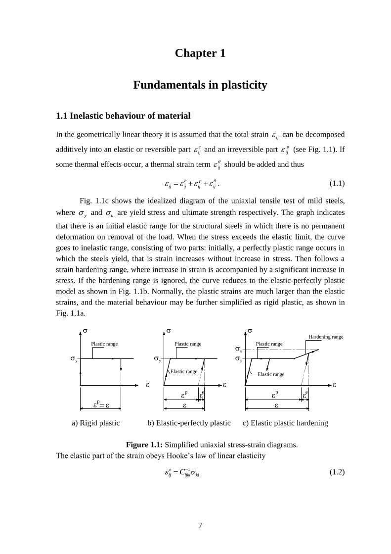
Fig. 1.1c shows the idealized diagram of the uniaxial tensile test of mild steels,

where y and u are yield stress and ultimate strength respectively. The graph indicates

that there is an initial elastic range for the structural steels in which there is no permanent

deformation on removal of the load. When the stress exceeds the elastic limit, the curve

goes to inelastic range, consisting of two parts: initially, a perfectly plastic range occurs in

which the steels yield, that is strain increases without increase in stress. Then follows a

strain hardening range, where increase in strain is accompanied by a significant increase in

stress. If the hardening range is ignored, the curve reduces to the elastic-perfectly plastic

model as shown in Fig. 1.1b. Normally, the plastic strains are much larger than the elastic

strains, and the material behaviour may be further simplified as rigid plastic, as shown in

Fig. 1.1a.

e

p

Plastic range

Hardening range

y

u

e

p

Elastic range

Plastic range

y

p

Plastic range

y

Elastic range

a) Rigid plastic b) Elastic-perfectly plastic c) Elastic plastic hardening

Figure 1.1: Simplified uniaxial stress-strain diagrams.

The elastic part of the strain obeys Hooke’s law of linear elasticity

1e

ij ijkl klC (1.2)

8

where the elastic constants ijklC are components of a tensor of rank 4. For an isotropic

material, this tensor is expressed in the form below

1 1 2 2 1ijkl ij kl ik jl il jk

E EC

(1.3)

where E denotes the Young’s modulus, the Poisson ratio, and ( , , , , )i j k l is the

Kronecker delta (Cartesian unit tensor of second order). The inverse relationship of (1.2)

can be written as

2

21 2

e e

ij ij ij kkG G

(1.4)

where

12

EG is the shear modulus of elasticity.

The plastic strain rate obeys an associated flow law

p f

εσ

(1.5)

where is a non-negative plastic multiplier and , ,f σ π represents a time-independent

yield surface, which will be discussed in the section 1.3.

1.2 Yield function-yield surface

To develop a mathematical theory of plasticity, a basic assumption is made that there exists

a continuous scalar yield function , ,f σ ξ , which has following properties:

The equation , , 0f σ ξ represents a convex hypersurface, called yield or

loading surface, in the stress space σ for a given temperature and an array of

internal variables ξ which are determined experimentally. The plastic strain

rate p

ε can be nonzero in the region where , , 0f σ ξ .

, , 0f σ ξ represents the elastic region, which occupies the interior of the

yield surface. In this region, both plastic strain rate p

ε and all internal variables

ξ are zeros.

, , 0f σ ξ corresponds to a region in stress space which is inaccessible for

the material.

For multi-axial stresses, it is necessary to define yield criteria which will cause

yielding. We present here after two most well-known yield criteria in plasticity. From

fig.1.1, we can see that the initial yielding is the same for the cases with or without

hardening.

9

According to Bridgman (1923), the plastic deformation of metals essentially is

independent of hydrostatic stress. Therefore only the deviatoric stress D

σ

1

tr3

D σ σ σ I (1.6)

causes yielding. Similarly we can express the strain deviator e as

1

tr3

e ε ε I . (1.7)

1.2.1 Von Mises yield criterion

The von Mises yield criterion is defined by the yield function

2

2 0vf J k σ (1.8)

where

vk is a material strength parameter. For a perfectly plastic material, vk is a

constant independent of strain history, for a hardening material vk will be

allowed to change with strain history.

2J is the second principal invariant of the stress deviator D

σ , which has the form1:

2

1:

2

D DJ σ σ . (1.9)

If the material is subjected to a pure shear 12, while all other stress components

vanish, then 2

2 12J , and yielding should occur when 12 vk . Hence the constant

3v yk is the yield stress in pure shear.

1.2.2 Tresca yield criterion

Tresca (1868) concluded that the decisive factor for yielding is the maximum shear stress

in the material. He proposed the yield criterion stipulating that the maximum shear stress

has a constant value during plastic flow.

Using the principal stresses 1 2 3, , is the simplest way to express Tresca’s idea.

If the principal axes of stress are so labelled that

1 2 3 , (1.10)

then Tresca’s yield condition is

1 3 2 0.Tf k (1.11)

1 For a general tensor σ this form is 2

2

1: tr

2I σ σ σ which the negative of the standard definition.

10

However, f in this form violates the rule that the manner in which the principal axes are

labelled 1, 2, 3 should not affect the form of the yield function. To obey this rule, we

observe that Tresca’s condition states that during plastic flow one of the differences

1 2 , 2 3 , 3 1 has the value 2 Tk . Hence we may write:

1 2 2 3 3 1, , 2 0Tf Max k σ , (1.12)

where 2

y

Tk

, y is yield stress. The equation (1.12) is now symmetrical with respect to

principal stresses, and can be put into an invariant form

3 2 2 2 4 6

2 3 2 3 2 2, 4 27 36 96 64 0T T Tf J J J J k J k J k , (1.13)

where 2 3, J J are the second and third invariants of the stress deviation tensor D

σ with 2J

given in (1.9), and

3

2 2 2

11 22 33 12 23 31 11 23 22 31 33 12

1det

3

2 .

D D D D

ij ij jk ki

D D D D D D

J

(1.14)

1.3 Perfect plasticity material and the initial yield surface

The yield function of perfectly plastic material, without hardening and temperature

dependence is

2 0yf F σ σ . (1.15)

For isotropic materials, the yield function depends only on the invariants of stress.

1 2 3, ,f f I I I (1.16)

where 1 2 3, ,I I I are the three invariants of the stress tensor ij . In terms of principal

stresses, the yield function is expressed as:

1 2 3, ,f f . (1.17)

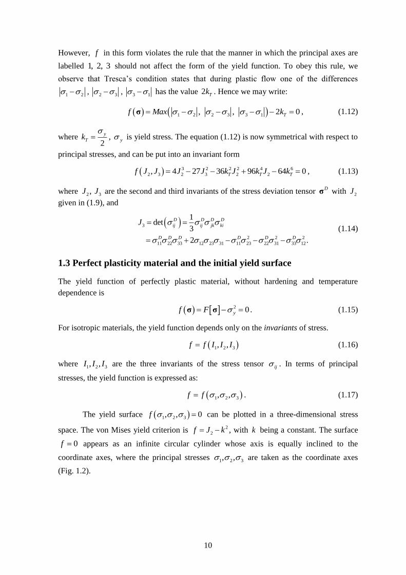
The yield surface 1 2 3, , 0f can be plotted in a three-dimensional stress

space. The von Mises yield criterion is 2

2f J k , with k being a constant. The surface

0f appears as an infinite circular cylinder whose axis is equally inclined to the

coordinate axes, where the principal stresses 1 2 3, , are taken as the coordinate axes

(Fig. 1.2).

11

1

2

3

1 2 3

Axis is the line

Yield surface

J - k = 02

2

Figure 1.2: Yield surface according to von Mises criterion

in the principal stress plane.

Since the effect of hydrostatic pressure on yield can be neglected, the yield function

will be independent of 1 1 2 3I . It means that the yield function could be

expressed advantageously as:

2 3,f f J J (1.18)

where 2 3,J J are the second and third invariants of the stress deviation tensor D

σ .

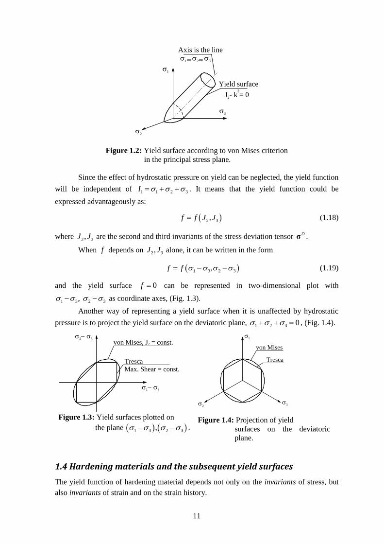
When f depends on 2 3,J J alone, it can be written in the form

1 3 2 3,f f (1.19)

and the yield surface 0f can be represented in two-dimensional plot with

1 3 2 3, as coordinate axes, (Fig. 1.3).

Another way of representing a yield surface when it is unaffected by hydrostatic

pressure is to project the yield surface on the deviatoric plane, 1 2 3 0 , (Fig. 1.4).

2 3

1 3

von Mises, J = const.

Tresca

2

Max. Shear = const.

Figure 1.3: Yield surfaces plotted on

the plane 1 3 2 3, .

1

2 3

von Mises

Tresca

Figure 1.4: Projection of yield

surfaces on the deviatoric

plane.

1.4 Hardening materials and the subsequent yield surfaces

The yield function of hardening material depends not only on the invariants of stress, but

also invariants of strain and on the strain history.

12

Obviously, we can model strain hardening by relating the size and shape of the

yield surface to plastic strain in some appropriate ways.

With the assumptions that the plastic deformation is independent of the hydrostatic

pressure and that the plastic flow is incompressible, the yield surface in the principal stress

space 1 2 3, , is a cylinder of infinite length and the axis 1 2 3 (see Fig. 1.2, the

cylinder is not necessary with circular cross section). The deviatoric plane, which has

1 2 3 0 is perpendicular to the axis 1 2 3 (Fig. 1.2). The yield surface can

be represented by its cross section on the plane 1 2 3 0 . The cross sectional curve

is closed convex, and piecewise smooth. It may change in size and shape during plastic

deformation. Hereafter, we present some hardening models based on hypotheses and

assumptions that approximate real behaviour more or less exactly (Fung & Pin Tong, 2001,

Lubliner, 2005).

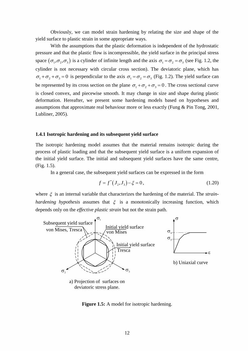
1.4.1 Isotropic hardening and its subsequent yield surface

The isotropic hardening model assumes that the material remains isotropic during the

process of plastic loading and that the subsequent yield surface is a uniform expansion of

the initial yield surface. The initial and subsequent yield surfaces have the same centre,

(Fig. 1.5).

In a general case, the subsequent yield surfaces can be expressed in the form

*

2 3, 0f f J J , (1.20)

where is an internal variable that characterizes the hardening of the material. The strain-

hardening hypothesis assumes that is a monotonically increasing function, which

depends only on the effective plastic strain but not the strain path.

1

2 3

Initial yield surface

Tresca

von Mises

Initial yield surface

Subsequent yield surface

von Mises, Tresca

u

y

a) Projection of surfaces on

deviatoric stress plane.

b) Uniaxial curve

Figure 1.5: A model for isotropic hardening.

13

An isotropic hardening law is generally not useful in situations where the structure

is subjected to cyclic loading. It does not account for the Bauschinger effect, and so it

predicts that after a few cycles the structure will just harden until it responds elastically.

This model rejects the possibility of incremental plasticity.

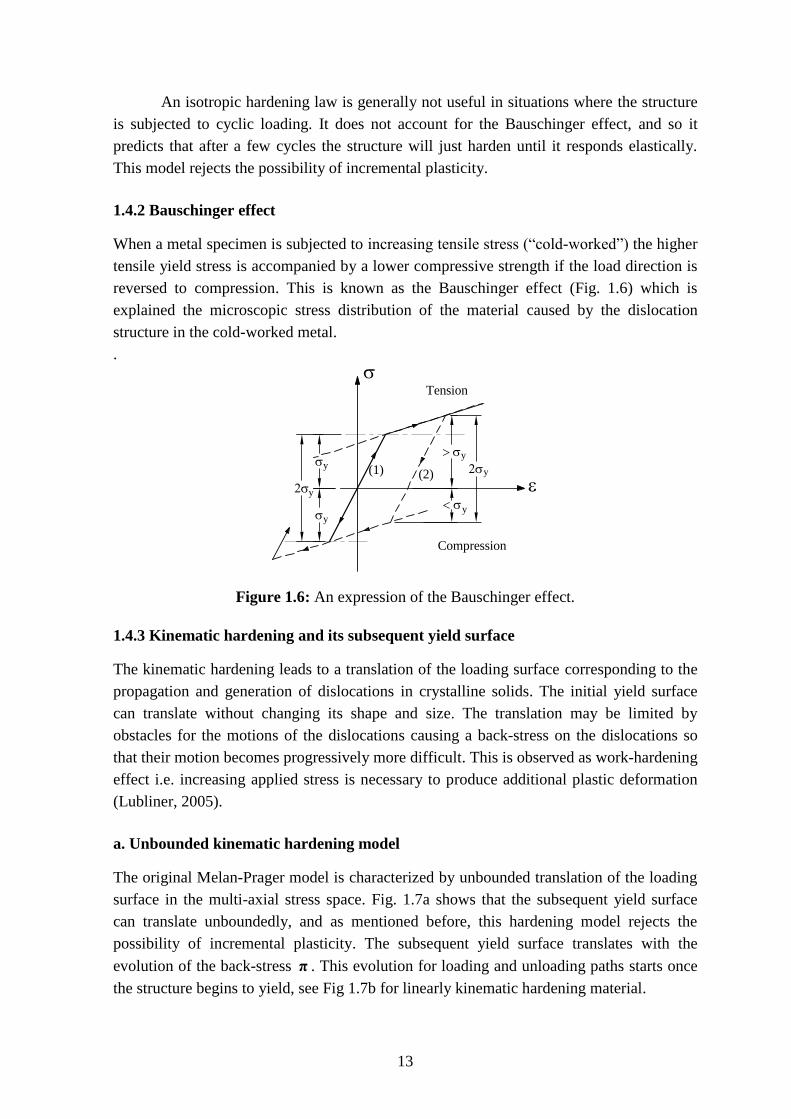
1.4.2 Bauschinger effect

When a metal specimen is subjected to increasing tensile stress (“cold-worked”) the higher

tensile yield stress is accompanied by a lower compressive strength if the load direction is

reversed to compression. This is known as the Bauschinger effect (Fig. 1.6) which is

explained the microscopic stress distribution of the material caused by the dislocation

structure in the cold-worked metal.

.

y

y

y

y

y

Compression

Tension

(1) (2)y

Figure 1.6: An expression of the Bauschinger effect.

1.4.3 Kinematic hardening and its subsequent yield surface

The kinematic hardening leads to a translation of the loading surface corresponding to the

propagation and generation of dislocations in crystalline solids. The initial yield surface

can translate without changing its shape and size. The translation may be limited by

obstacles for the motions of the dislocations causing a back-stress on the dislocations so

that their motion becomes progressively more difficult. This is observed as work-hardening

effect i.e. increasing applied stress is necessary to produce additional plastic deformation

(Lubliner, 2005).

a. Unbounded kinematic hardening model

The original Melan-Prager model is characterized by unbounded translation of the loading

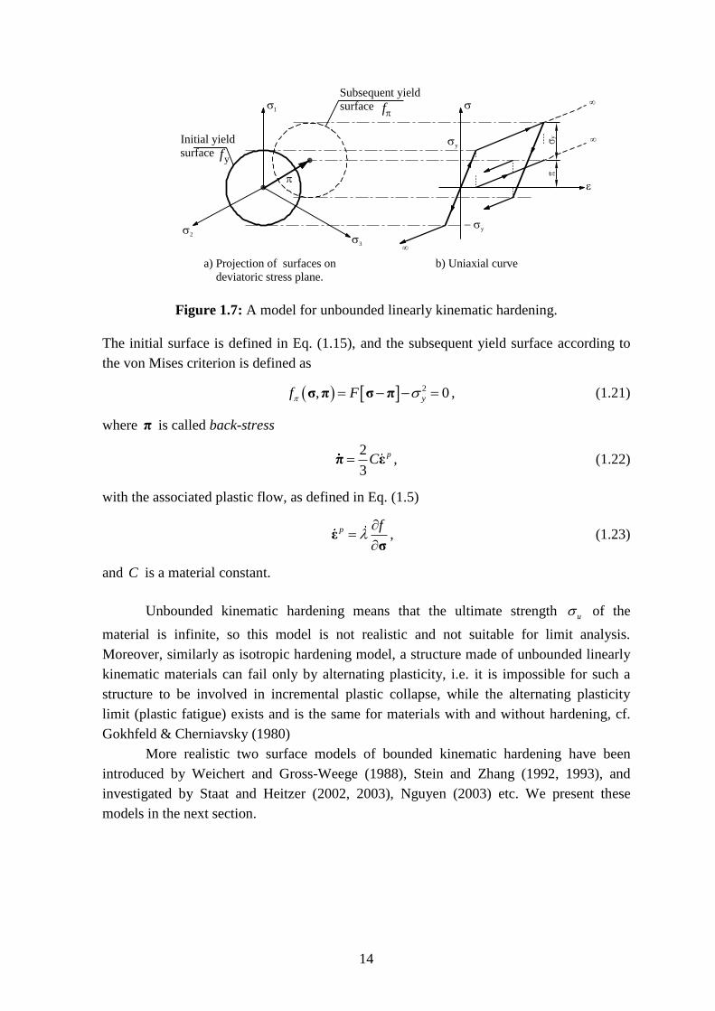
surface in the multi-axial stress space. Fig. 1.7a shows that the subsequent yield surface

can translate unboundedly, and as mentioned before, this hardening model rejects the

possibility of incremental plasticity. The subsequent yield surface translates with the

evolution of the back-stress π . This evolution for loading and unloading paths starts once

the structure begins to yield, see Fig 1.7b for linearly kinematic hardening material.

14

Subsequent yield

surface

Initial yield

surface

f1

2

3

y


deviatoric stress plane.

b) Uniaxial curve

y

y

yf

Figure 1.7: A model for unbounded linearly kinematic hardening.

The initial surface is defined in Eq. (1.15), and the subsequent yield surface according to

the von Mises criterion is defined as

2, 0yf F σ π σ π , (1.21)

where π is called back-stress

2

3

pCπ ε , (1.22)

with the associated plastic flow, as defined in Eq. (1.5)

p f

εσ

, (1.23)

and C is a material constant.

Unbounded kinematic hardening means that the ultimate strength u of the

material is infinite, so this model is not realistic and not suitable for limit analysis.

Moreover, similarly as isotropic hardening model, a structure made of unbounded linearly

kinematic materials can fail only by alternating plasticity, i.e. it is impossible for such a

structure to be involved in incremental plastic collapse, while the alternating plasticity

limit (plastic fatigue) exists and is the same for materials with and without hardening, cf.

Gokhfeld & Cherniavsky (1980)

More realistic two surface models of bounded kinematic hardening have been

introduced by Weichert and Gross-Weege (1988), Stein and Zhang (1992, 1993), and

investigated by Staat and Heitzer (2002, 2003), Nguyen (2003) etc. We present these

models in the next section.

15

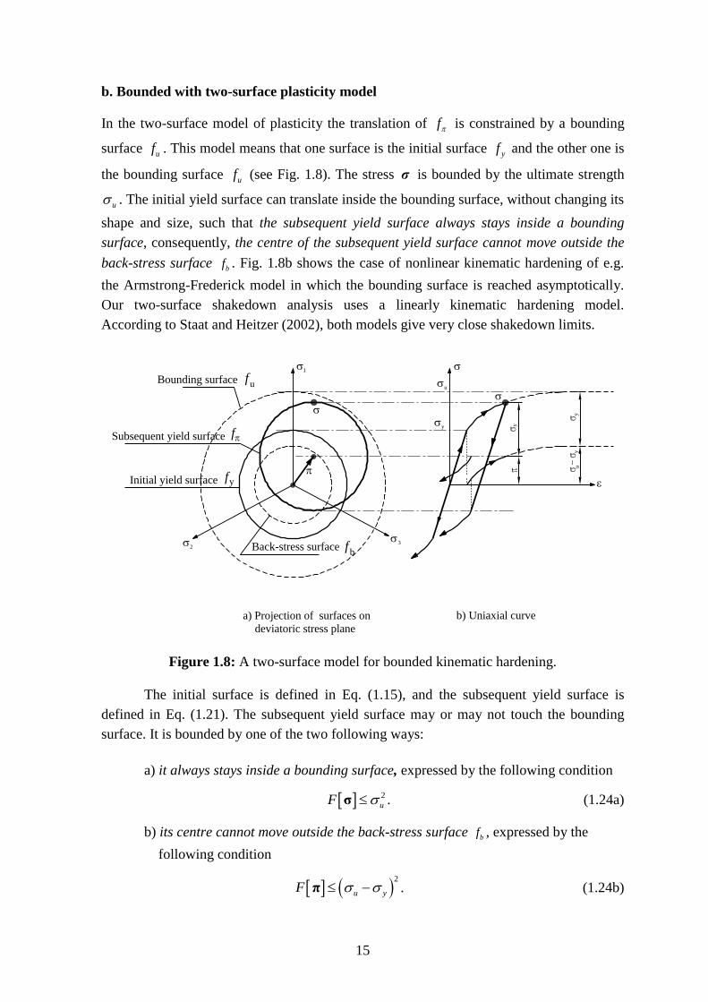
b. Bounded with two-surface plasticity model

In the two-surface model of plasticity the translation of f is constrained by a bounding

surface uf . This model means that one surface is the initial surface yf and the other one is

the bounding surface uf (see Fig. 1.8). The stress σ is bounded by the ultimate strength

u . The initial yield surface can translate inside the bounding surface, without changing its

shape and size, such that the subsequent yield surface always stays inside a bounding

surface, consequently, the centre of the subsequent yield surface cannot move outside the

back-stress surface bf . Fig. 1.8b shows the case of nonlinear kinematic hardening of e.g.

the Armstrong-Frederick model in which the bounding surface is reached asymptotically.

Our two-surface shakedown analysis uses a linearly kinematic hardening model.

According to Staat and Heitzer (2002), both models give very close shakedown limits.

1

23

Subsequent yield surface

Bounding surface

y

u


deviatoric stress plane

b) Uniaxial curve

fu

f

yu

y

Back-stress surface fb

y

Initial yield surface fy

Figure 1.8: A two-surface model for bounded kinematic hardening.

The initial surface is defined in Eq. (1.15), and the subsequent yield surface is

defined in Eq. (1.21). The subsequent yield surface may or may not touch the bounding

surface. It is bounded by one of the two following ways:

a) it always stays inside a bounding surface, expressed by the following condition

2

uF σ . (1.24a)

b) its centre cannot move outside the back-stress surface bf , expressed by the

following condition

2

u yF π . (1.24b)

16

In Eqs. (1.24a) and (1.24b), inequality presents the subsequent yield surface does not touch

the bounding surface.

Intuitively, from Fig. 1.8, we can see that conditions (1.24a) and (1.24b) are equivalent,

otherwise, it is easily proved.

Firstly, we prove: (1.24a) (1.24b) . From the triangle inequality

y u y uF F F F σ σ π π σ π π (a)

, andy

y u y

u y

FF F

F

σ πσ π π

π (b)

then

22

u u yF F πσ . (Q.E.D.) (1.25)

Finally, we prove: (1.24b) (1.24a) .

If we choose u y

u

π σ so that y

u

σ π σ . Then for any σ satisfying 2

uF σ

we will find:

2

2u y u y

u y

u u

F F F

σπ σ (c)

From (c) and π chosen before, we have

2

2 2y y

y u

u u

F F F F

σσ π σ σ (d)

then

2

2 .u y uF F π σ (Q.E.D.) (1.26)

Some authors such as Zhang G. (1991), Pham D. C. (2005, 2007) use condition

(1.24a). Other authors like Weichert, Groß-Weege (1988), Heitzer, Staat (2003) use

(1.24b).2 Zhang G. (1991, pp. 43-44) argues that

2

u yF π is safer than

2

uF σ . The above prove however shows that both conditions are equivalent.

Zhang (1991), Heitzer and Staat (2003) have proved that when 2u y then

shakedown limit of bounded kinematic hardening structure is equal to that of unbounded

2 Heitzer (1999) has proven that the optimization problems of lower bound shakedown analysis based on

either constraint (1.24a) or (1.24b) have the same solution. The above prove is independent of shakedown

analysis.

17

kinematic hardening structure. Gokhfeld & Cherniavsky (1980) also stated that the

problem of alternating plasticity can be solved directly by using the fictitious elastic field

Eσ . It is due to the fact that the plastic fatigue limit is determined by the condition that

anywhere in the structure; the maximum magnitude of fictitious equivalent (von Mises)

elastic stress cannot exceed two times the yield limit of the material. Moreover, intuitively,

from Fig. 1.6, the evolution of the initial yield surface takes place within the range of 2 y .

1.5 Drucker’s postulate

Drucker’s postulates were developed in the 1950s in an attempt to provide the missing link

between material behaviour and mathematics, (see Bower, 2010).

The process of application and removal of the additional stress is called stress

cycle. Removing the additional stress enables the stress of the structure to return to the

original stress state, but the strain state can be different if plastic deformation occurred

during the stress cycle. Note that : ed dσ ε is always positive, where d eε is the elastic strain

increment which is recoverable. Drucker (Fung & Pin Tong, 2001) accordingly defines a

work-hardening (or “stable”) plastic material if the following two conditions hold true.

the work done during incremental loading is positive

: 0; andd d σ ε (1.27)

the work done in the loading-unloading cycle is nonnegative

: : 0e pd d d d d σ ε ε σ ε (1.28)

where pdε is the plastic strain increment, which is not recovered by the process of stress

cycle. Eq. (1.28) sometimes known simply as Drucker’s inequality, is valid for both

work-hardening and perfectly plastic materials, where for perfect plasticity, it assumes

equality: : : 0p pd d σ ε σ ε .

Drucker (Fung & Pin Tong, 2001) extended the definition of work-hardening to

allow for a finite dσ produced by the external agency. In fact, the initial stress, 0

σ , may

not at any point be outside the yield surface such that 0 σ σ . The work per unit volume

done by the external agency is 0 : pdσ σ ε . Eq. (1.28) is replaced by

0 : 0p σ σ ε . (1.29)

Equation (1.29) is also called the principle of maximum plastic dissipation. It can be

written in the form

0: , :p p pD σ ε ε ξ σ ε , (1.30)

18

where the plastic dissipation ,pD ε ξ depends on the plastic strain rate p

ε and the

internal variable ξ only. The back-stress is a suitable internal variable, i.e. ξ π .

Consequences of Drucker’s postulate

The yield surface and all subsequent loading surfaces must be convex.

The convexity of the yield surface plays a very important role in plasticity. It

permits the use of convex programming in limit and shakedown analysis. It should be

noted that Drucker’s postulate is quite independent of the basic laws of thermodynamics. It

does not hold if internal structural changes occur or for temperature dependent behaviour

(Kalisky, 1985). Furthermore, the yield surface fails to be convex if there is an interaction

between elastic and plastic deformations, i.e. if the elastic properties depend on the plastic

deformation (Panagiotopoulos, 1985).

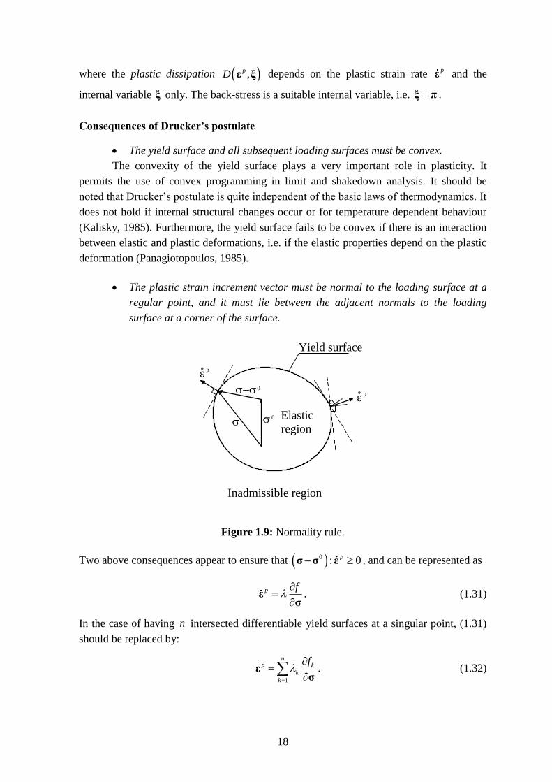
The plastic strain increment vector must be normal to the loading surface at a

regular point, and it must lie between the adjacent normals to the loading

surface at a corner of the surface.

Yield surface

Elastic

region

Inadmissible region

p

0

0

p

Figure 1.9: Normality rule.

Two above consequences appear to ensure that 0 : 0p σ σ ε , and can be represented as

p f

εσ

. (1.31)

In the case of having n intersected differentiable yield surfaces at a singular point, (1.31)

should be replaced by:

1

np k

k

k

f

ε

σ. (1.32)

19

The rate of change of plastic strain must be a linear function of the change of

the stress.

1.6 Plastic dissipation functions

The plastic dissipation function is defined in Eq. (1.30)

, :p pD ε π σ ε (1.33)

σ is the existing stress tensor satisfying the yield condition , 0f σ π . Hereafter, we will

express the dissipation function of the initial yield surface, of the subsequent surface, and

of the bounding surface according to the von Mises criterion. As mentioned before, the

effect hydrostatic stress can be neglected in metal plasticity, (see Eq. (1.6) and Eq. (1.7)).

1.6.1 Initial surface

The initial yield surface is defined in Eq. (1.15)

2 0y yf f F σ σ (1.34)

For the von Mises criterion it can be described as follows

3

2: 0D D

y yf σ σ . (1.35)

The dissipation function corresponding to (1.35) is defined as

2

3: :p p p p p

yD ε σ ε ε ε . (1.36)

It is quite clear that if there is no evolution of the initial surface, then the initial

yield surface is exactly the yield surface of a perfectly plastic material.

The total plastic strain rate p

ε can be separated into two components, König (1987)

, , ,p p p

ut t t ε x ε x ε x . (1.37)

The first term of Eq. (1.37) represents a perfectly incremental collapse process over

a time interval 0,T , in which a kinematically admissible plastic strain increment uε x

is attained in a proportional and monotonic way

0

, , (a)

, ,0 is kinematically admissible (b)

, 0 , , 1

u u

u u u

T

t t

T

t t dt

ε x x ε x

ε x ε x ε x

x x (c)

(1.38)

and the second term of Eq. (1.37) represents an alternating plasticity process

20

0

,

T

p p t dt ε x ε x 0 . (1.39)

Obviously this alternating plasticity process should correspond to an alternating stress

process for an isotropic material.

1.6.2 Subsequent yield surface

The subsequent yield surface (translated surface) is defined in Eq. (1.21)

2, 0yf f F σ π σ π . (1.40)


3

2: 0D D

yf σ π σ π . (1.41)


2

3: :p p D p p p

yD ε σ π ε ε ε . (1.42)

As mentioned in Eq. (1.37), p

ε involves only alternating plasticity (or LCF).

1.6.3 Bounding surface

The bounding surface is defined in Eq. (1.24a)

2 0u uf f F σ σ . (1.43)


3

2: 0D D

u uf σ σ . (1.44)


2

3: :p p p p p

u u u u uD ε σ ε ε ε . (1.45)

As mentioned in Eq. (1.37), p

uε involves to ratchetting or incremental plastic collapse.

when f is bounded by uf , correspondingly, its centre cannot move outside the back-

stress surface bf which is defined in Eq. (1.24b)

2

b u yf f F π π . (1.46)

For the von Mises criterion it can be described as follow

3

2: 0b u yf π π . (1.47)

21


23

p

u y

V

dV ε , (1.48)

where

0

T

p pdt ε ε . (1.49)

As proved in the last section, bounding conditions (1.43) and (1.46) are equivalent.

1.6.4 Total internal dissipation energy of bounded linearly kinematic hardening

Since the initial yield surface translates inside the bounding surface during the load cycles,

so the dissipation of the subsequent yield surface depends not only on the stress but also on

the strain history- Then it is more convenient to define the dissipation function for any case

of shakedown (see Eq. (1.50)) than for a certain case such as either alternating (see Eq.

(1.42)) or ratchetting (see Eq. (1.45)), (see Nguyen Q.S (2003)).

2 23 3

0 0

T T

p p p p

y u y

V V V

D dVdt dVdt dV ε ε ε . (1.50)

On the right hand side of Eq. (1.50), the first term is the internal plastic energy of a

structure made of perfectly plastic material, and the second term is the effect of hardening.

1.7 Fundamental principles in plasticity

Consider a structure subjected to volume loads (body force) f and surface loads 0t . The

stresses σ are said to be in equilibrium if they satisfy the equations of internal equilibrium

in div V σ f 0 (1.51)

and the conditions of equilibrium on the traction boundary V of the body

0 on V σn t . (1.52)

Any stress field satisfying conditions (1.51) and (1.52) is called a statically admissible

field. Furthermore, if this stress field nowhere violates the yield criterion, 0f σ , it is

called a plastically admissible or licit stress field.

The actual flow mechanism is composed of the velocities u and strain rate ε in the

body which satisfy the compatibility condition and kinematical boundary conditions

1 in ,

2

TV ε u u (1.53)

0 on uV u u . (1.54)

Any mechanism ,u ε satisfying conditions (1.53) and (1.54) is called kinematically

22

admissible. Furthermore, if this mechanism furnishes a non negative external power3

0 0T T

ex

V V

W dV dS

f u t u (1.55)

then it is called a licit mechanism. A kinematically admissible strain and displacement field

can be defined in a similar manner.

Principle of virtual power

One of the main tools in the mechanics of continua is the principle of virtual power,

which states that for an arbitrary set of virtual velocity variations u that are

kinematically admissible, the necessary and sufficient condition to make the stress field σ

equilibrium is to satisfy the following variational equation

0: T T

V V V

dV dV dS

σ ε f u t u . (1.56)

Principle of complimentary virtual power

For an arbitrary set of virtual variations of the stress tensor σ that are statically

admissible, the necessary and sufficient condition to make the strain rate tensor ε and

velocity vector u compatible is to satisfy the following variational equation

:

u

T

V V

dV dS

ε σ n σ u . (1.57)

Equation of virtual power

From the two above principles, one can easily deduce that for all strain rate tensors

ε and velocity vectors u that are kinematically admissible, and for all stresses σ that are

statically admissible we have the following virtual power equation

0 0:

u

TT T

V V V V

dV dV dS dS

σ ε f u t u nσ u . (1.58)

In the above variational principles no constitutive equation of the material is

assumed. Variational Eqs. (1.56) and (1.57) are applicable even if the body is not elastic,

for which the energy functional cannot be defined. The finite element analysis of structures

is based on these variational equations.

3 The notation of the product T f u assumes matrix notation in Cartesian coordinates. In tensor notation the

transposition has no effect and we could simply write i if u f u .

23

Chapter 2

Limit analysis

2.1 Introduction

In this chapter we only present the basic theory of limit analysis but not all details because

we will state that limit analysis is a special case of shakedown analysis in next chapters.

Let us consider a structure of volume V made of ideal plastic or bounded

hardening material and subjected to external loading P . The external loading P consists

of general body force f in V and surface traction t on V . The bar (horizontal line)

placed over the loads f and t implies that these loads are time-independent. We assume

that:

The material is ductile so that the structure can undergo large deformations

beyond elastic limit without fracture.

The deflections of the structure under loading are small so that second-order

effects can be ignored. Therefore buckling cannot be considered in limit analysis.

All loads are applied in a monotonic and proportional way, i.e.

0P P (2.1)

where 0 0 0,P f t denotes the nominal or initial load. If the value of the load factor is

sufficiently small, the structure behaves elastically. As increases and reaches a special

value, the first point in the structure reaches the plastic state. This state of stress is called

elastic limit. The corresponding load factor is denoted el . Further increase of will lead

to the expansion of plastic regions in the structure. The structure gradually reduces the

statically indeterminacy (redundancy). At limit state, the structure forms a collapse

mechanism and therefore fails to carry the applied load. If 0P represents the applied load,

the value lim corresponding to the plastic collapse state is called the safety factor of the

structure or the limit load multiplier.

The theory of limit analysis offers a way to solve directly the problem of estimating

the plastic collapse load limP , bypassing the spreading process of the plastic flow. The limit

value of the load is estimated and at the same time the limit state of stress in the whole

structure can be evaluated. The limit load and stresses so obtained are of great interest in

practical engineering whenever the model of perfect plasticity or bounded hardening and

the small deformation and small displacement assumption constitute a good approximation

of the material.

24

2.2 Definition of licit fields

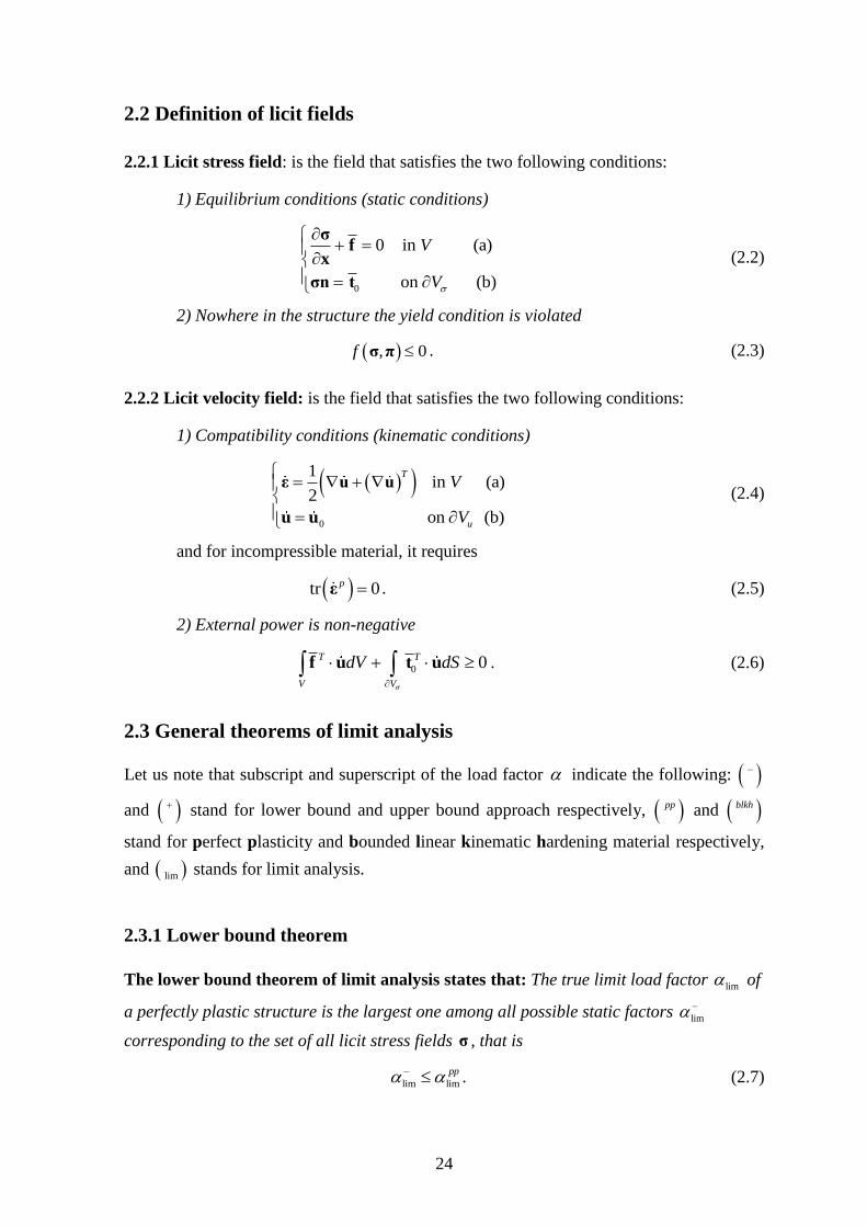
2.2.1 Licit stress field: is the field that satisfies the two following conditions:

1) Equilibrium conditions (static conditions)

0

0 in (a)

on (b)

V

V

σf

x

σn t

(2.2)

2) Nowhere in the structure the yield condition is violated

, 0f σ π . (2.3)

2.2.2 Licit velocity field: is the field that satisfies the two following conditions:

1) Compatibility conditions (kinematic conditions)

0

1 in (a)

2

on (b)

T

u

V

V

ε u u

u u

(2.4)

and for incompressible material, it requires

tr 0p ε . (2.5)

2) External power is non-negative

0 0T T

V V

dV dS

f u t u . (2.6)

2.3 General theorems of limit analysis

Let us note that subscript and superscript of the load factor indicate the following:

and stand for lower bound and upper bound approach respectively, pp and blkh

stand for perfect plasticity and bounded linear kinematic hardening material respectively,

and lim stands for limit analysis.

2.3.1 Lower bound theorem

The lower bound theorem of limit analysis states that: The true limit load factor lim of

a perfectly plastic structure is the largest one among all possible static factors lim

corresponding to the set of all licit stress fields σ , that is

lim lim

pp . (2.7)

25

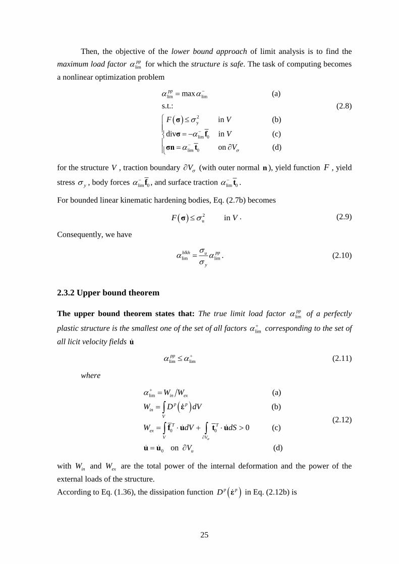
Then, the objective of the lower bound approach of limit analysis is to find the

maximum load factor lim

pp for which the structure is safe. The task of computing becomes

a nonlinear optimization problem

lim lim

2

y

lim 0

lim 0

max (a)

s.t.:

in (b)

div in (c)

on (d)

pp

F V

V

V

σ

σ f

σn t

(2.8)

for the structure V , traction boundary V (with outer normal n ), yield function F , yield

stress y , body forces lim 0 f , and surface traction lim 0

t .

For bounded linear kinematic hardening bodies, Eq. (2.7b) becomes

2

u in F Vσ . (2.9)

Consequently, we have

lim lim

blkh ppu

y

. (2.10)

2.3.2 Upper bound theorem

The upper bound theorem states that: The true limit load factor lim

pp of a perfectly

plastic structure is the smallest one of the set of all factors lim corresponding to the set of

all licit velocity fields u

lim lim

pp (2.11)

where

lim

0 0

0

(a)

(b)

0 (c)

on

in ex

p p

in

V

T T

ex

V V

u

W W

W D dV

W dV dS

V

ε

f u t u

u u (d)

(2.12)

with inW and exW are the total power of the internal deformation and the power of the

external loads of the structure.

According to Eq. (1.36), the dissipation function p pD ε in Eq. (2.12b) is

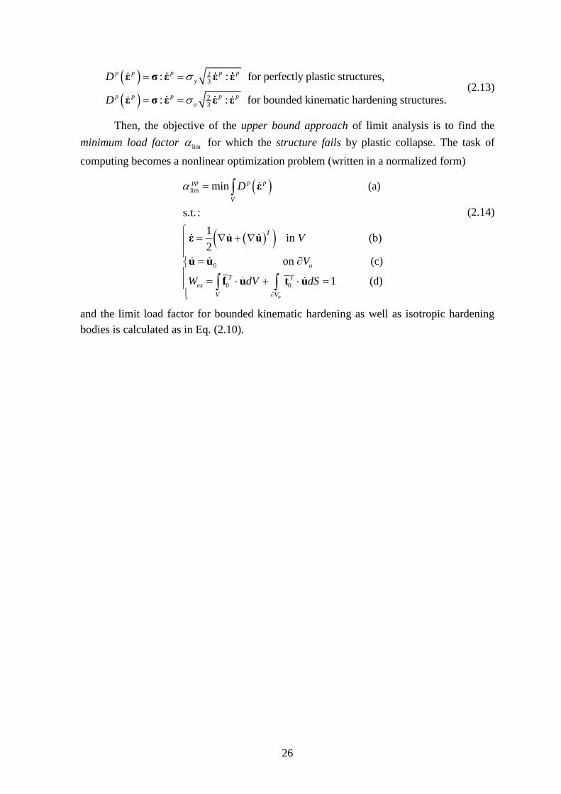
26

23

23

: : for perfectly plastic structures,

: : for bounded kinematic hardening structures.

p p p p p

y

p p p p p

u

D

D

ε σ ε ε ε

ε σ ε ε ε

(2.13)

Then, the objective of the upper bound approach of limit analysis is to find the

minimum load factor lim for which the structure fails by plastic collapse. The task of

computing becomes a nonlinear optimization problem (written in a normalized form)

lim

0

0 0

min (a)

s.t. :

1 in (b)

2

on (c)

1

pp p p

V

T

u

T T

ex

V V

D

V

V

W dV dS

ε

ε u u

u u

f u t u (d)

(2.14)

and the limit load factor for bounded kinematic hardening as well as isotropic hardening

bodies is calculated as in Eq. (2.10).

27

Summary

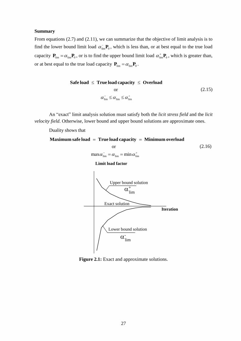
From equations (2.7) and (2.11), we can summarize that the objective of limit analysis is to

find the lower bound limit load lim 0 P , which is less than, or at best equal to the true load

capacity lim lim 0P P , or is to find the upper bound limit load lim 0 P , which is greater than,

or at best equal to the true load capacity lim lim 0P P .

lim lim lim

or

Safe load True load capacity Overload

(2.15)

An “exact” limit analysis solution must satisfy both the licit stress field and the licit

velocity field. Otherwise, lower bound and upper bound solutions are approximate ones.

Duality shows that

lim lim lim

or

max min

Maximum safe load True load capacity Minimum overload

(2.16)

Upper bound solution

Lower bound solution

Exact solution

Iteration

Limit load factor

lim+

lim-

Figure 2.1: Exact and approximate solutions.

29

Chapter 3

Shakedown theories

3.1 Behaviour of a structure

For structures subjected to varying loads, shakedown is more relevant than static collapse,

which has been investigated by limit analysis in the last chapter. A structure made of

perfectly plastic materials as well as linear or nonlinear kinematic hardening materials,

subjected to cyclic loads may behave in one of the following ways, depending on the

intensity and character of the applied loads.

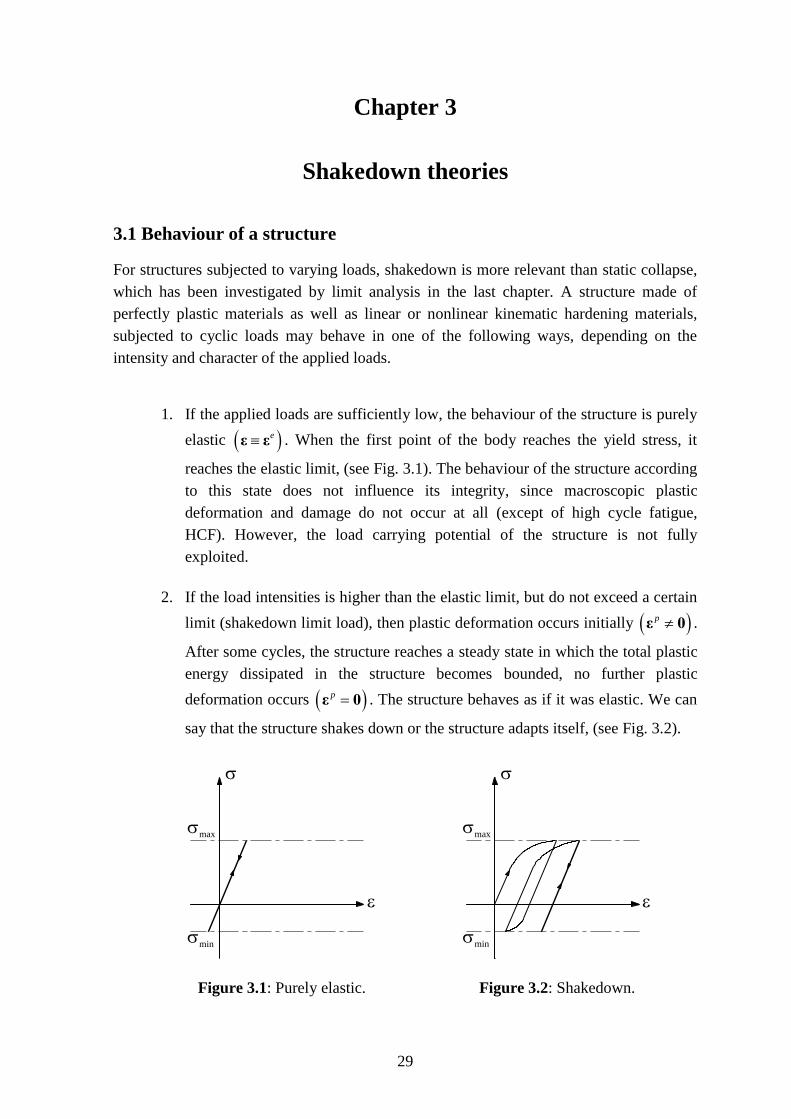
1. If the applied loads are sufficiently low, the behaviour of the structure is purely

elastic eε ε . When the first point of the body reaches the yield stress, it

reaches the elastic limit, (see Fig. 3.1). The behaviour of the structure according

to this state does not influence its integrity, since macroscopic plastic

deformation and damage do not occur at all (except of high cycle fatigue,

HCF). However, the load carrying potential of the structure is not fully

exploited.

2. If the load intensities is higher than the elastic limit, but do not exceed a certain

limit (shakedown limit load), then plastic deformation occurs initially p ε 0 .

After some cycles, the structure reaches a steady state in which the total plastic

energy dissipated in the structure becomes bounded, no further plastic

deformation occurs p ε 0 . The structure behaves as if it was elastic. We can

say that the structure shakes down or the structure adapts itself, (see Fig. 3.2).

max

min

Figure 3.1: Purely elastic.

min

max

Figure 3.2: Shakedown.

30

3. If the load intensity is higher than the shakedown limit, then no stabilization

situation is established, plastic flow continues to develop. The response of the

structure may be one of the two following modes (or both simultaneously):

If the plastic strain increments in each load cycle, p ε 0 , are of the

same sign, the plastic deformations in each cycle accumulates, p ε 0 ,

so that after enough cycles the total strains (and therefore displacements)

become so large that the structure departs from its original form and

becomes unserviceable. This phenomenon is called incremental collapse or

ratchetting (see Fig. 3.3).

If the plastic strain increments change sign in every cycle p ε 0 , they

tend to cancel each other pε 0 , and the net deformation remains small.

However, after a sufficient number of cycles, the structure may fail by

fracture due to Low Cycle Fatigue (LCF). This phenomenon is called

alternating plasticity or low cycle fatigue, (see Fig. 3.4). Hardening does not

affect this state.

max

min

Figure 3.3: Ratchetting.

max

min

Figure 3.4: Alternating plasticity.

Note that: (1) incremental collapse and alternating plasticity may appear

simultaneously, and (2) in the alternating plasticity mode, there is no essential difference

between elastic-perfectly plastic and kinematic hardening materials.

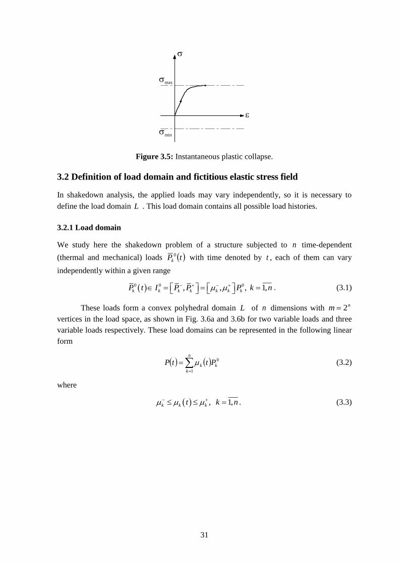
4. If the load intensity is higher than the ultimate strength capacity of the structure,

limP P , then the structure collapses instantaneously. This collapse is relevant

to static collapse (see Fig. 3.5). The ultimate strength capacity of the structure

made of unbounded kinematic hardening material is infinite.

31

max

min

Figure 3.5: Instantaneous plastic collapse.

3.2 Definition of load domain and fictitious elastic stress field

In shakedown analysis, the applied loads may vary independently, so it is necessary to

define the load domain L . This load domain contains all possible load histories.

3.2.1 Load domain

We study here the shakedown problem of a structure subjected to n time-dependent

(thermal and mechanical) loads tPk

0 with time denoted by t , each of them can vary

independently within a given range

0 0 0, , , 1,k k k k k k kP t I P P P k n . (3.1)

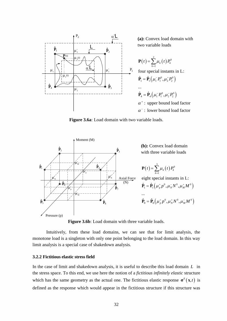
These loads form a convex polyhedral domain L of n dimensions with nm 2

vertices in the load space, as shown in Fig. 3.6a and 3.6b for two variable loads and three

variable loads respectively. These load domains can be represented in the following linear

form

n

k

kk PttP1

0 (3.2)

where

, 1,k k kt k n . (3.3)

32

P1^

P2^

P3^P4

^

P

P

2

11

+1

-

2

+

2

-

L+

L-

L

P(t)

2(t)

1(t)

(a): Convex load domain with

two variable loads

20

1

0 0

1 1 1 1 2 2

0 0

4 4 1 1 2 2

four special instants in :

ˆ ˆ ,

...

ˆ ˆ ,

: upper bound load factor

: lower bound load factor

k k

k

t t P

P P

P P

P

P P

P P

L

Figure 3.6a: Load domain with two variable loads.

M

+

M

-

p

-

N

- N

+

p

+

Moment (M)

Axial Force

(N)

Pressure (p)

P1^

P2^

P3^

P7^

P8^P5

^

P6^

P4^

(b): Convex load domain

with three variable loads

30

1

0 0 0

1 1

0 0 0

8 8

eight special instants in :

ˆ ˆ , ,

...

ˆ ˆ , ,

k k

k

p N M

p N M

t t P

p N M

p N M

P

P P

P P

L

Figure 3.6b: Load domain with three variable loads.

Intuitively, from these load domains, we can see that for limit analysis, the

monotone load is a singleton with only one point belonging to the load domain. In this way

limit analysis is a special case of shakedown analysis.

3.2.2 Fictitious elastic stress field

In the case of limit and shakedown analysis, it is useful to describe this load domain L in

the stress space. To this end, we use here the notion of a fictitious infinitely elastic structure

which has the same geometry as the actual one. The fictitious elastic response ,E tσ x is

defined as the response which would appear in the fictitious structure if this structure was

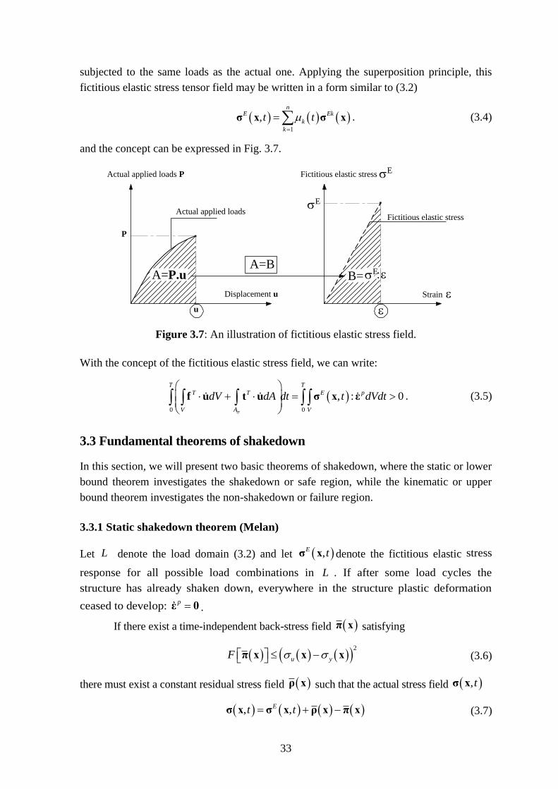
33

subjected to the same loads as the actual one. Applying the superposition principle, this

fictitious elastic stress tensor field may be written in a form similar to (3.2)

1

,n

E Ek

k

k

t t

σ x σ x . (3.4)

and the concept can be expressed in Fig. 3.7.

Displacement u

Actual applied loads

Actual applied loads P

Strain

Fictitious elastic stress

Fictitious elastic stress

A=P.u B=

u

P

E

EA=B

E

Figure 3.7: An illustration of fictitious elastic stress field.

With the concept of the fictitious elastic stress field, we can write:

0 0

, : 0

T T

T T E p

V A V

dV dA dt t dVdt

f u t u σ x ε . (3.5)

3.3 Fundamental theorems of shakedown

In this section, we will present two basic theorems of shakedown, where the static or lower

bound theorem investigates the shakedown or safe region, while the kinematic or upper

bound theorem investigates the non-shakedown or failure region.

3.3.1 Static shakedown theorem (Melan)

Let L denote the load domain (3.2) and let ,E tσ x denote the fictitious elastic stress

response for all possible load combinations in L . If after some load cycles the

structure has already shaken down, everywhere in the structure plastic deformation

ceased to develop: p ε 0 .

If there exist a time-independent back-stress field π x satisfying

2

u yF π x x x (3.6)

there must exist a constant residual stress field ρ x such that the actual stress field ,tσ x

, ,Et t σ x σ x ρ x π x (3.7)

34

does not anywhere violate the yield criterion:

2,E

yF t σ x ρ x π x x (3.8)

The following theorem shows that this is the necessary and sufficient condition for a

structure to shake down (for perfect plasticity see Koiter 1960):

Theorem 3.1:

Shakedown occurs if there exists a permanent residual stress field ρ x , statically

admissible, such that:

2,E

yF t σ x ρ x π x x (3.9)

Shakedown will not occur if no ρ x exists such that

2,E

yF t σ x ρ x π x x . (3.10)

Based on the above static theorem, we can find a permanent statically admissible

residual stress field in order to obtain a maximum load domain that guarantees (3.10).

The obtained shakedown load multiplier sd is generally a lower bound. The shakedown

problem can be seen as a maximization issue in nonlinear programming

2

2

max (a)

s.t.:

, , (b)

(c)

div

sd

E

y

u y

F t V t

F V

σ x ρ x π x x x

π x x x x

ρ x

(d)

(e)

V

V

0 x

ρ x n 0 x

(3.11)

For the perfectly plastic behaviour u y , the back-stresses π are identical

zero due to the second inequality (3.11c). Melan’s original theorem for unbounded

kinematic hardening can be also deduced from the previous formulation if u . Then

the second inequality is not relevant anymore and the back-stresses π are free variables.

3.3.2 Kinematic shakedown theorem (Koiter)

Using plastic strain fields to formulate shakedown criterion, the kinematic shakedown

theorem is the counterpart of the static one. The theorem was given by Koiter (1960) and

some of its applications in analysis of incremental collapse were derived by Gokhfeld

(1980), Sawczuk (1969a, b). The same as proposed by Koiter for plastic strain field, we

introduce here an admissible cycle of the plastic strain field pε , corresponding to a cycle

of the displacement field u . The plastic strain rate p

ε may not necessarily be compatible

35

at each instant during the time cycle T but the plastic strain accumulation over the cycle

defined below

0

T

p pdt ε ε (3.12)

must be compatible, such that

12

in (a)

on (b)

Tp

u

V

V

ε u u

u 0

(3.13)

Theorem 3.2:

The structure will shake down if

0 0

, :

T T

E p p p

V V

t dVdt D dVdt σ x ε ε . (3.14)

The structure will not shake down if

0 0

, :

T T

E p p p

V V


For the bounded kinematic hardening model, (see section 1.5.4), we have:

2 23 3

0 0

T T

p p p p

y u y

V V V

D dVdt dVdt dV ε ε ε . (3.16)

In equation (3.16), u y is the penalty parameter associated with the constraint

0p ε , where pε is defined in Eq. (3.12).

The first term on the right hand side of Eq. (3.16) is exactly the total dissipation

energy of perfectly plastic structures, while the second term takes the hardening effect into

account. It is quite clear that:

If u y , it is the perfectly plastic behavior

If alternating plasticity occurs, which means p ε 0 , then the right hand side

of Eq. (3.16) retains only the first term. Again like the perfectly plastic

behavior, then

blkh pp

alternating alternating (3.17)

The conclusion (3.17) has been stated in literature, e.g. Gokhfeld &

Cherniavsky (1980), Stein & Huang (1995), Pham D.C. (2007).

For limit analysis, Eq. (3.16) can be rewritten as

36

2 23 3

23

p p p p

y u y

V V V

p

u

V

D dV dV dV

dV

ε ε ε

ε (3.18)

Then

lim lim

blkh ppu

y

. (3.19)

Based on the kinematic theorem, an upper bound of the shakedown limit load

multiplier sd can be computed. The shakedown problem can be seen as a mathematical

minimization problem of nonlinear programming

0

0

0

12

min (a)

, :

s.t. :

(b)

in (c)

T

p p

Vsd T

E p

V

T

p p

Tp

D dVdt

t dVdt

dt

V

ε

σ x ε

ε ε

ε u u

u 0 on (d)uV

(3.20)

As presented before, there are two modes of shakedown: alternating plasticity or

low cycle fatigue (LCF), and incremental plasticity or ratchetting. Equation (3.20b) is the

definition of accumulated plastic strain. If p ε 0 then LCF occurs, else if

p ε 0 , then

ratchetting occurs. We can calculate LCF and ratchetting limits separately or

simultaneously by separated shakedown method or unified shakedown method

respectively. The next section presents these methods.

3.4 Methods of calculating LCF limit and ratchetting limit

3.4.1 Separated shakedown method

This method defines the LCF limit and the ratchetting limit separately. As presented in

Chapter 1, Eqs (1.37) to (1.39), any plastic strain history ,p tε x can be separated into two

components

, , ,p p p

ut t t ε x ε x ε x , (3.21)

where ,p

u tε x involves ratchetting, and ,p tε x involves LCF. There are three

possibilities (cf. Pham D. C., (2005))

37

1) , and , : ratchetting appears

2) , and , : LCF appears

3) , and , : ratchetting and LCF appear simultaneously

p p

u

p p

u

p p

u

t t

t t

t t

ε x 0 ε x 0

ε x 0 ε x 0

ε x 0 ε x 0

These possible modes can be defined precisely in the following way

1. A perfect incremental collapse process (over a certain time interval T,0 ) is a

process of plastic deformation ,p

u tε x in which a kinematically admissible

plastic strain increment , , ,0p p p

u u ut T ε x ε x ε x is attained in a

proportional and monotonic way, namely

12

in (a)

on (b)

, (c)

, 0

Tp

u

u

p p

u u

V

V

t

t

ε u u

u 0

ε x ε x

x

(d)

,0 0 (e)

, 1 (g)T

x

x

(3.22)

2. An alternating plasticity process is any process of plastic deformation ,p tε x

within a certain time interval T,0 such that the total increment of the plastic

strain p

ε x over this period is zero,

0

,

T

p p t dt ε x ε x 0 . (3.23)

Based on the upper bound theorem, the criteria of safety with respect to incremental

collapse may be obtained by substituting the plastic strain history (3.22) into the

shakedown condition (3.14) with the dissipation (1.45), then it leads to (cf. Pham D. C.

(2005, 2007)).

Theorem 3.3a:

The incremental collapse will not happen if

0 0

, :

T T

E p p p

u u

V V


The incremental collapse will happen if

38

0 0

, :

T T

E p p p

u u

V V

t dVdt D dVdt σ x ε ε (3.25)

with

2

3

0

1

2

: : (a)

, (b)

in (c)

on

p p p p p

u u u u u

T

p p

u u

Tp

u

u

D

t dt

V

V

ε σ ε ε ε

ε x ε x 0

ε u u

u 0 (d)

(3.26)

and the criteria of safety with respect to LCF may be obtained by substituting the plastic

strain history (3.23) into the shakedown condition (3.14) with the dissipation (1.42), then it

leads to (cf. Pham D.C. (2005, 2007))

Theorem 3.3b:

The alternating plasticity will not happen if

0 0

, :

T T

E p p p

V V


The alternating plasticity will happen if

0 0

, :

T T

E p p p

V V


with

2

3

0

: : (a)

, (b)

p p p p p

y

T

p p

D

t dt

ε σ ε ε ε

ε x x 0 (3.29)

3.4.1.1 Incremental collapse criterion

If the safety condition against any form of perfectly incremental collapse is considered, the

plastic strain field is assumed by (3.22). Substituting (3.22) into (3.24), one obtains

0 0

, ,

T T

E p p p

ex u in u

V V

W t t dVdt W D dVdt σ x x ε x ε . (3.30)

By taking into account the properties of the dissipation function and the plastic

strain history (3.22), we can write

39

0 0

T T

p p p p p p

in u u u

V V V

W D dVdt dt D dV D dV ε ε ε . (3.31)

From the shakedown condition (3.30), the smallest upper bound of incremental

limit could be attained when the external power exW assumes its maximum and the internal

dissipation inW takes its minimum. To this end, the function ),( tx is selected in such a

way that 0),( tx only when the product ,E ut σ x ε x takes its maximum possible

value for a given load domain L . In this case, the external power exW can be written as

0

, , : :

T

E p E p

ex u u

V V

W t t dVdt dV σ x x ε x σ x ε x (3.32)

in which

: max , :E p E p

u ut σ x ε x σ x ε x . (3.33)

By this way, the safety condition against any form of perfectly incremental collapse

thus has the form

:E p p p

u u

V V

dV D dV σ x ε x ε . (3.34)

If the load variation domain is prescribed by (3.2), (3.3) and (3.4), namely n

independently varying loads, the formulation (3.34) becomes

1

:n

Ek p p p

k u u

kV V

dV D dV

σ x ε x ε (3.35)

in which

if : 0

if : 0

Ek p

k u

k Ek p

k u

σ x ε x

σ x ε x (3.36)

From condition (2.34), the shakedown load multiplier against incremental collapse

sd can be formulated as a non-linear minimization problem

min insd

ex

W

W

(3.37)

or in normalized form

min

s.t.: 1

sd in

ex

W

W

(3.38)

40

3.4.1.2 Alternating plasticity criterion

If the safety condition against alternating plasticity is considered, the plastic strain field

must be satisfied (3.23). The shakedown condition (3.27) in this case has the form

0 0

, : ,

T T

E p p p

V V

t t dVdt D dVdt σ x ε x ε (3.39)

with

0

1, , for all

T

p t dt V ε x 0 x . (3.40)

Starting from the kinematic theorem and the last constraint in (3.40), the

optimization problem leading to the most stringent limit condition can be established at

each point x separately. The global safety factor against alternating plasticity limit will be

the minimum of local ( ) x defined as

0

0

0

1max , : ,

s.t.:

1

,

T

E p

T

p p

T

p

t t dt

D dt

t dt

ε

σ x ε xx

ε

ε x 0

(3.41)

By solving this problem, the static shakedown condition against any form of

alternating plasticity can be obtained.

A given structure is safe against alternating plasticity if there exists a time-

independent stress field ρ which, if superimposed on the envelope of elastic stresses, does

not violate the yield condition

, 0Ef t σ x ρ x π x . (3.42)

It should be noted that the stress field ρ in (3.42) is an arbitrary time-independent

stress field and not necessarily self-equilibrated as it is required in Melan’s theorem (3.9)

and (3.10). We define a general stress response

*

1

nEk

k k

k

σ x σ x π x (3.43)

where Ekσ x and π x are the elastic stress field and back-stress field respectively in the

reference structure when subjected to the k th load and

, 2 2

k k k kk k

. (3.44)

41

In view of (3.41), the plastic shakedown load multiplier (lower bound) may be calculated

as

*

1min

F

x σ x ρ x π x (3.45)

where

1f F . (3.46)

The sign of k must be chosen so that the value of function F is maximal. By

considering the alternating characteristic of the stress corresponding to an alternating strain

rate, the optimal time-independent stress field ρ can be defined by

1

nEk

k

k

ρ σ π . (3.47)

Then the plastic shakedown limit load multiplier can be finally represented as

1

1min

nEk

k

k

F

x

σ x π x

. (3.48)

3.4.2 Unified shakedown method

This method defines the LCF limit and the ratchetting limit simultaneously. It is not

necessary to separate the plastic strain history ,p tε x into two components ,p

u tε x and

,p tε x as presented in Eq. (3.17). Then theorems 3.3a and 3.3b for the upper bound

approach can be re-stated as, (see Nguyen Q-S. (2003)):

Theorem 3.4

The necessary and sufficient condition for shakedown to occur is that there exists a

plastic accumulation mechanism p such that

2 23 3

0 0

0

, :

compatible

T T

E p p p

y u y

V V V

T

p p

t dVdt dVdt dV

dt

σ x ε ε ε

ε ε

(3.49)

In computations, in most cases it is not practicable to apply lower and upper bound

theorems in their above form to find directly the shakedown limit defined by the minimum

of the incremental plasticity limit and alternating plasticity limit. The difficulty here, for

the lower bound approach is the presence of the time-dependent stress field ,E tσ x in

(3.9) and (3.10) and the theorems are stated only for time-independent residual stress ρ x

42

and time-independent back-stress π x , and for upper bound approach the difficulty is

appearance of the time integration in equation (3.20). These obstacles can be overcome

with the discretization of the load domains, which will be presented in next chapter.

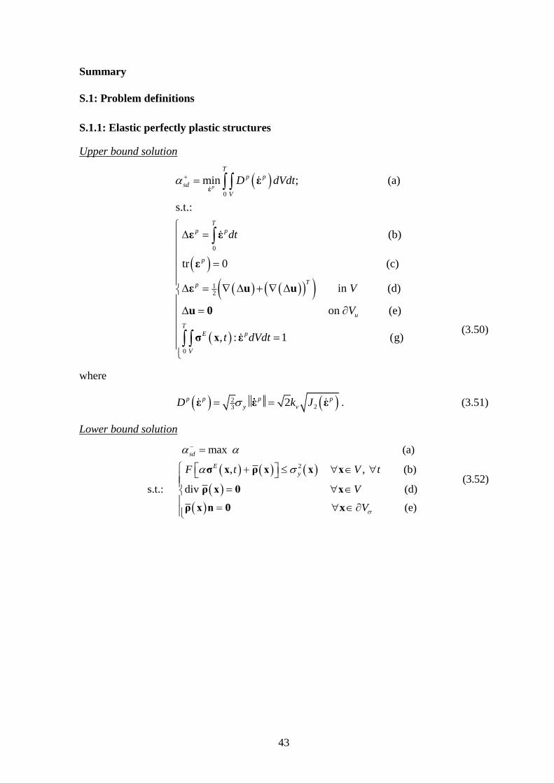
43

Summary

S.1: Problem definitions

S.1.1: Elastic perfectly plastic structures


0

0

min ; (a)

s.t.:

(b)

tr 0 (c)

p

T

p p

sd

V

T

p p

p

p

D dVdt

dt

εε

ε ε

ε

ε

12

0

in (d)

on (e)

, : 1 (g)

T

u

T

E p

V

V

V

t dVdt

u u

u 0

σ x ε (3.50)

where

223

2p p p p

y vD k J ε ε ε . (3.51)


2

max (a)

, , (b)

s.t.: div (d)

sd

E

yF t V t

V

σ x ρ x x x

ρ x 0 x

ρ x n (e)V

0 x

(3.52)

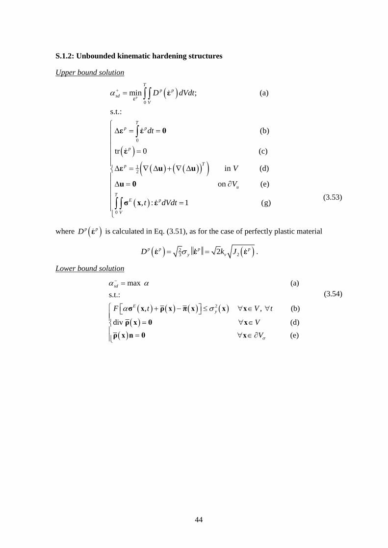
44

S.1.2: Unbounded kinematic hardening structures


0

0

12

min ; (a)

s.t.:

(b)

tr 0 (c)

p

T

p p

sd

V

T

p p

p

p

D dVdt

dt

εε

ε ε 0

ε

ε

0

in (d)

on (e)

, : 1 (g)

T

u

T

E p

V

V

V

t dVdt

u u

u 0

σ x ε (3.53)

where p pD ε is calculated in Eq. (3.51), as for the case of perfectly plastic material

223

2p p p p

y vD k J ε ε ε .


2

max (a)

s.t.:

, , (b)

div

sd

E

yF t V t

V

σ x ρ x π x x x

ρ x 0 x

(d)

(e)V

ρ x n 0 x

(3.54)

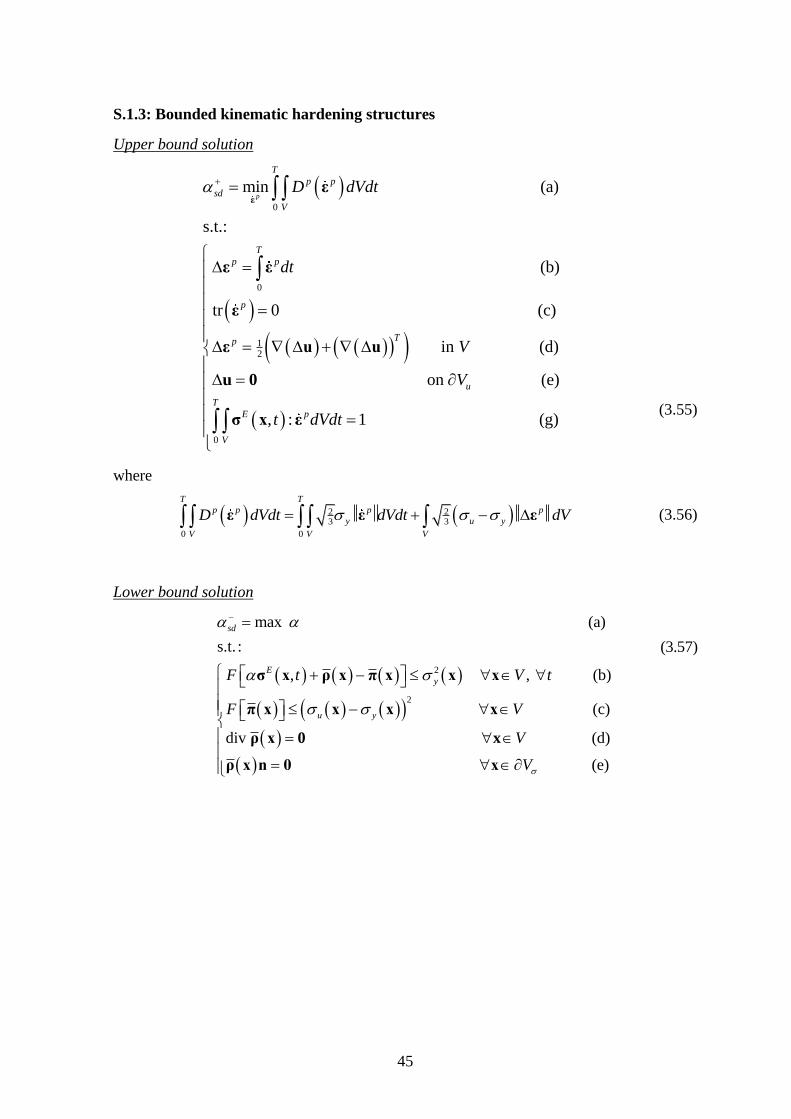
45

S.1.3: Bounded kinematic hardening structures


0

0

min (a)

s.t.:

(b)

tr 0

p

T

p p

sd

V

T

p p

p

D dVdt

dt

εε

ε ε

ε

12

0

(c)

in (d)

on (e)

, : 1 (g)

Tp

u

T

E p

V

V

V

t dVdt

ε u u

u 0

σ x ε

(3.55)

where

2 23 3

0 0

T T

p p p p

y u y

V V V

D dVdt dVdt dV ε ε ε (3.56)


2

2

max (a)

s.t. :

, , (b)

(c)

div

sd

E

y

u y

F t V t

F V

σ x ρ x π x x x

π x x x x

ρ x

(d)

(e)

V

V

0 x

ρ x n 0 x

(3.57)

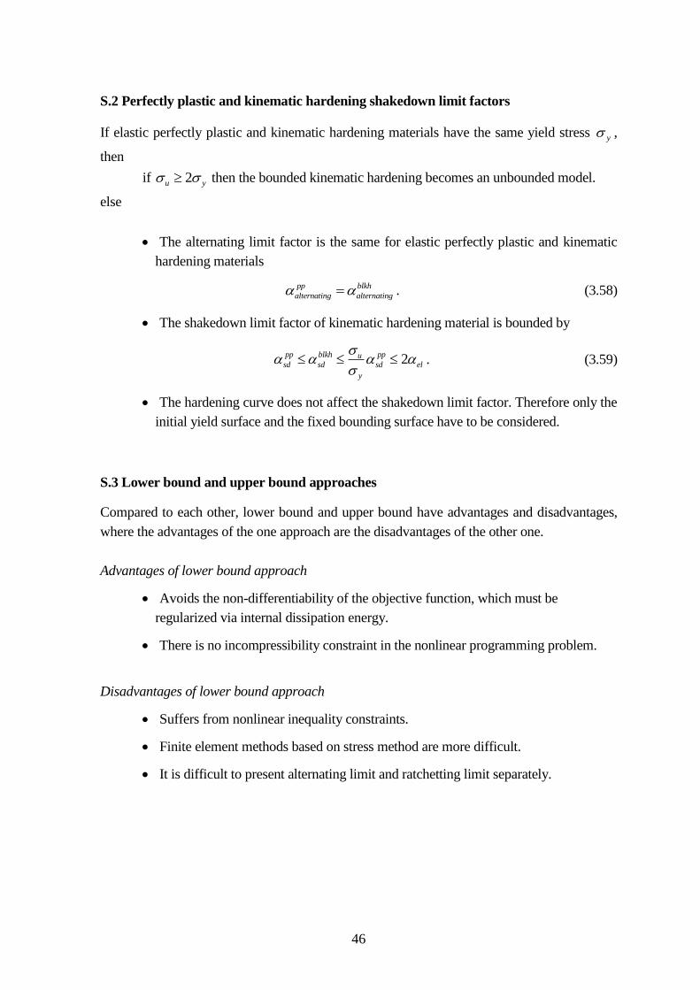
46

S.2 Perfectly plastic and kinematic hardening shakedown limit factors

If elastic perfectly plastic and kinematic hardening materials have the same yield stress y ,

then

if 2u y then the bounded kinematic hardening becomes an unbounded model.

else

The alternating limit factor is the same for elastic perfectly plastic and kinematic

hardening materials

pp blkh

alternating alternating . (3.58)

The shakedown limit factor of kinematic hardening material is bounded by

2pp blkh ppusd sd sd el

y

. (3.59)

The hardening curve does not affect the shakedown limit factor. Therefore only the

initial yield surface and the fixed bounding surface have to be considered.

S.3 Lower bound and upper bound approaches

Compared to each other, lower bound and upper bound have advantages and disadvantages,

where the advantages of the one approach are the disadvantages of the other one.

Advantages of lower bound approach

Avoids the non-differentiability of the objective function, which must be

regularized via internal dissipation energy.

There is no incompressibility constraint in the nonlinear programming problem.

Disadvantages of lower bound approach

Suffers from nonlinear inequality constraints.

Finite element methods based on stress method are more difficult.

It is difficult to present alternating limit and ratchetting limit separately.

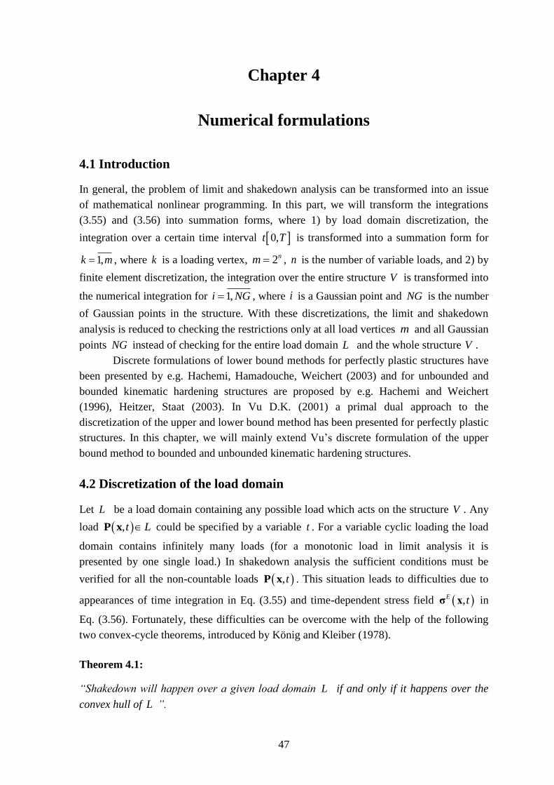
47

Chapter 4

Numerical formulations

4.1 Introduction

In general, the problem of limit and shakedown analysis can be transformed into an issue

of mathematical nonlinear programming. In this part, we will transform the integrations

(3.55) and (3.56) into summation forms, where 1) by load domain discretization, the

integration over a certain time interval 0,t T is transformed into a summation form for

1,k m , where k is a loading vertex, 2nm , n is the number of variable loads, and 2) by

finite element discretization, the integration over the entire structure V is transformed into

the numerical integration for 1,i NG , where i is a Gaussian point and NG is the number

of Gaussian points in the structure. With these discretizations, the limit and shakedown

analysis is reduced to checking the restrictions only at all load vertices m and all Gaussian

points NG instead of checking for the entire load domain L and the whole structure V .

Discrete formulations of lower bound methods for perfectly plastic structures have

been presented by e.g. Hachemi, Hamadouche, Weichert (2003) and for unbounded and

bounded kinematic hardening structures are proposed by e.g. Hachemi and Weichert

(1996), Heitzer, Staat (2003). In Vu D.K. (2001) a primal dual approach to the

discretization of the upper and lower bound method has been presented for perfectly plastic

structures. In this chapter, we will mainly extend Vu’s discrete formulation of the upper

bound method to bounded and unbounded kinematic hardening structures.

4.2 Discretization of the load domain

Let L be a load domain containing any possible load which acts on the structure V . Any

load ,t P x L could be specified by a variable t . For a variable cyclic loading the load

domain contains infinitely many loads (for a monotonic load in limit analysis it is

presented by one single load.) In shakedown analysis the sufficient conditions must be

verified for all the non-countable loads ,tP x . This situation leads to difficulties due to

appearances of time integration in Eq. (3.55) and time-dependent stress field ,E tσ x in

Eq. (3.56). Fortunately, these difficulties can be overcome with the help of the following

two convex-cycle theorems, introduced by König and Kleiber (1978).

Theorem 4.1:

“Shakedown will happen over a given load domain L if and only if it happens over the

convex hull of L ”.

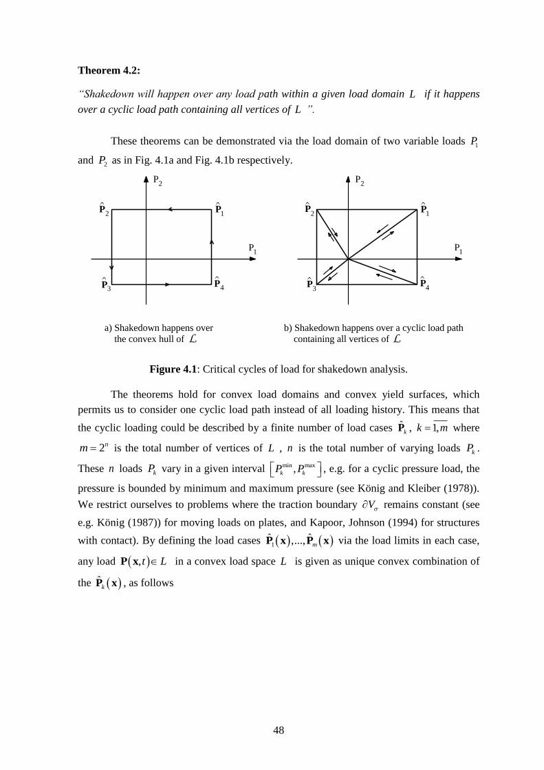
48

Theorem 4.2:

“Shakedown will happen over any load path within a given load domain L if it happens

over a cyclic load path containing all vertices of L ”.

These theorems can be demonstrated via the load domain of two variable loads 1P

and 2P as in Fig. 4.1a and Fig. 4.1b respectively.

Figure 4.1: Critical cycles of load for shakedown analysis.

The theorems hold for convex load domains and convex yield surfaces, which

permits us to consider one cyclic load path instead of all loading history. This means that

the cyclic loading could be described by a finite number of load cases ˆkP , 1,k m where

2nm is the total number of vertices of L , n is the total number of varying loads kP .

These n loads kP vary in a given interval min max,k kP P , e.g. for a cyclic pressure load, the

pressure is bounded by minimum and maximum pressure (see König and Kleiber (1978)).

We restrict ourselves to problems where the traction boundary V remains constant (see

e.g. König (1987)) for moving loads on plates, and Kapoor, Johnson (1994) for structures

with contact). By defining the load cases 1ˆ ˆ,..., mP x P x via the load limits in each case,

any load ,t P x L in a convex load space L is given as unique convex combination of

the ˆkP x , as follows

^2

^3

P̂4

^1

P1

P2

^2

^3

^4

^1

P1

P2

PP

P

P P

PP

a) Shakedown happens over

the convex hull of

b) Shakedown happens over a cyclic load path

containing all vertices of L L

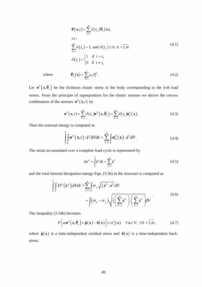
49

1

1

ˆ, ,

s.t.:

1, and 0, 1,

1 if

0 if

m

k k

k

m

k k

k

k

k

k

t t

t t k m

t tt

t t

P x P x

(4.1)

where 0

1

ˆn

k k k

k

P

P x . (4.2)

Let ˆ,E

kσ x P be the fictitious elastic stress in the body corresponding to the k-th load

vertex. From the principle of superposition for the elastic stresses we derive the convex

combination of the stresses ,E tσ x by

1 1

ˆ, ,m m

E E E

k k k k

k k

t t t

σ x σ x P σ x . (4.3)

Then the external energy is computed as

10

, : :

T mE p E k

k

kV V

t dVdt dV

σ x ε σ x ε . (4.4)

The strain accumulated over a complete load cycle is represented by

10

T mp p k

k

dt

ε ε ε (4.5)

and the total internal dissipation energy Eqn. (3.56) in the structure is computed as

23

10

23

1 1

= :

:

T mp p k k

y

kV V

m mk k

u y

k kV

D dVdt dV

dV

ε ε ε

ε ε

. (4.6)

The inequality (3.54b) becomes

2ˆ, , 1,E

k yF V k m

σ x P ρ x π x x x , (4.7)

where ρ x is a time-independent residual stress and π x is a time-independent back-

stress.

50

4.3 FEM discretizations

From the consequence of load domain discretization, in the next section we only consider

all load vertices ˆkP x of the load domain L instead of ,tP x . And from now on, all

quantities are time-independent ones.

4.3.1 Discrete formulation of lower bound method

To calculate the fictitious elastic stresses E

kσ in the reference body EV which is the same

as the original body V , subjected to the same loading ˆkP in the load domain L , we use

the virtual work principle combined with the finite element discretization with shape

functions for the displacement fields. Then, the fictitious elastic stresses E

kσ are in

equilibrium with body forces kf and surface tractions kt if the following equality holds

:

u

T E T T

k k k k k k

V V V

dV dV dS

ε σ u f u t (4.8)

for any virtual displacement u and any virtual strains ε satisfying the compatibility

condition.

12

in (a)

on (b)

T

u

V

V

ε u u

u 0

(4.9)

The virtual displacement field u within each element e is approximated by interpolation

of nodal values:

1

NDe

l l

l

u N u (4.10)

where lN and e

lu denote respectively the l -th shape function matrix and the vector of

virtual displacements of the l -th node of the finite element e which has ND nodes. The

virtual strain field is derived as follows

e e ε u N u B x u . (4.11)

Here B x N is the deformation matrix. Eq. (4.11) is called strain-displacement

relation or relation of lower bound and upper bound method.

By means of the finite element method, the structure V can be discretized into ne elements

eV , the integration (4.8) is subdivided into the integrations over each element e .

1 1 1

ngne neeT E e

i i ik k

e i e

w

B σ f (4.12)

where

51

E e e e e e

ik k i k σ E ε E B u (4.13)

ng is the total number of Gaussian points in each element e , iw is the weight factor at

Gaussian point i , e

iB is the deformation matrix at Gaussian point i of element e , E

ikσ is

fictitious elastic stress vector at Gaussian point i corresponding to load vertex ˆkP , e

kf is

the vector of nodal loads of element e corresponding to vertex ˆkP , e

E is the matrix of

elastic moduli of element e . Here e

iB and eE are the two constant matrices for any load

vertex.

Eq. (4.12) can be written in the following form

1 1

NG neT E e

i i ik k

i e

w

B σ f (4.14)

where NG ng ne is total number of Gaussian points in the structure.

Simultaneously, we can write the equilibrium equation (4.14) for residual stress as

1

NGT T

i i i

i

w

B ρ B ρ 0 . (4.15)

Equation (4.15) is numerical form replaced for derivative form of Eq. (3.57d & 3.57e),

where B and ρ are the global deformation matrix and the global residual stress vector,

respectively. They have the following form

1 1 2 2

1 2

, ,..., ,..., (a)

, ,..., ,..., (b)

i i NG NG

T T T T T

i NG

w w w w

B B B B B

ρ ρ ρ ρ ρ (4.16)

With the discretized residual stresses ρ calculated at Gaussian points only, the discretized

necessary limit and shakedown conditions are derived with the yield stress ,y i at every

Gaussian point i . Eq. (4.7) becomes

2

,

E

ik i i y iF σ ρ π . (4.17)

The restrictions of the optimization problems are checked only at the Gaussian points.

Finally, the shakedown limit load factor for bounded kinematic hardening

structures based on the lower bound approach, which is expressed in Eq. (3.57), becomes

52

2

,

2

, ,

max (a)

s.t.:

1, , 1, (b)

1,

sd

E

ik i i y i

i u i y i

F i NG k m

F i NG

σ ρ π

π

1

(c)

1, (d)NG

T T

i i i i

i

w i NG

B ρ B ρ 0

(4.18)

Here E

ikσ is calculated in Eq. (4.14). The problem (4.18) has 2 1NSC NG unknowns:

, , and i i ρ π , NG inequality constraints for yield condition, NG inequality constraints for

bounding condition, and NSC NG equality constraints for equilibrium condition, where

NG is number of Gaussian points of structure, NSC is number of stress components of each

Gaussian point.

4.3.2 Discrete formulation of upper bound method

As in the lower bound discretization, the structure V is subdivided into ne elements eV ,

the integration (4.6) of the internal dissipation energy can be written as

2 23 3

1 1 1

2 23 3

1 1 1 1 1

: + :

: :

e e

m m mk k k k

y u y

k k kV V

m ne ne m mk k k k

y e u y e

k e e k kV V

dV dV

dV dV

ε ε ε ε

ε ε ε ε

(4.19)

Using the Gauss-Legendre integration technique, the integration over the e-th element eV

is approximated by numerical integration, Eq. (4.19) can be transformed into

2 23 3

1 1 1 1 1

2 23 3

1 1 1 1 1 1 1

23

1 1

: + :

: :

:

e e

ne m ne m mk k k k

y e u y e

e k e k kV V

ng ngm ne ne m mik ik ik ik

i y i u y

k e i e i k k

NG mik ik

i y i u

i k

dV dV

w w

w w

ε ε ε ε

ε ε ε ε

ε ε 23

1 1 1

:NG m m

ik ik

y

i k k

ε ε

(4.20)

Similarly, the integration (4.7) of the external energy can be written as

1 1 1 1 1 1

1 1

: : :

:

e

ngm m ne m neE k E k E ik

k k e i ik

k k e k e iV V

m NGE ik

i ik

k i

dV dV w

w

σ x ε σ x ε σ ε

σ ε

(4.21)

53

in the above equations, ik

ε is the strain tensor and E

ikσ is the fictitious elastic stress tensor

at Gaussian point i and load vertex k .

In order to avoid the singularity of the dissipation function (4.20), we introduce

here a very small value 2

0 , where 2

00 1 , such that

2203

1 10

2203

1 1 1

:

: .

T NG mp p ik ik

i y

i kV

NG m mik ik

i u y

i k k

D dVdt w

w

ε ε ε

ε ε

(4.22)

From now onwards we work with matrix notations instead of tensor notations but

without changing the symbols. The functions of the strain tensor ikε , Eq. (4.22) can be

written as,

2203

1 10

2203

1 1 1

T NG mp p

i y ik ik

i kV

NG m m

i u y ik ik

i k k

D dVdt w

w

ε ε Dε

ε D ε

(4.23)

where ikε is the strain vector corresponding to load vertex ˆkP , at Gaussian point i

11 22 33 12 23 13

11 22 33 12 23 13

2 2 2

Tik ik ik ik ik ik

ik

Tik ik ik ik ik ik

ε (4.24)

and D is a diagonal square matrix. In a three-dimensional model, D has the form as

1 1 11 1 1

2 2 2Diag

D . (4.25)

The external energy in Eq.(4.21) can be rewritten as function of vectors of strain ikε as:

1 10

, :

T m NGE p T E

i ik ik

k iV

t dVdt w

σ x ε ε σ . (4.26)

The strain accumulation, which has been defined in Eq. (3.55b), must be compatible at

each Gaussian point i . Eqs. (3.55 b, d, e) then becomes

1

m

ik i

k

ε B u . (4.27)

And the incompressibility condition (3.55c) can be expressed in vector form

M ik D ε 0 (4.28)

where MD is a square matrix. In a three-dimensional problem, it has the following form

54

1 1 1 0 0 0

1 1 1 0 0 0

1 1 1 0 0 0

0 0 0 0 0 0

0 0 0 0 0 0

0 0 0 0 0 0

M

D . (4.29)

Finally, with the load domain and finite element discretization, the optimization

problem for the shakedown limit load factor for bounded kinematic hardening structures

based on the upper bound approach presented in Eq. (3.55) becomes

2 2 2203

1 1

2 2 2203

1 1 1

1

min

(a)

s.t. :

1,

p

m NGT

blkh y i ik ik i

k i

NG m mT

u y i ik ik i

i k k

m

ik i

k

w w

w w

i NG

εε Dε

ε D ε

ε B u

1 1

(b)

1, , 1, (c)

1

M ik

m NGT E

i ik ik

k i

i NG k m

w

D ε 0

ε σ (d)

(4.30)

Once again, as mention with respect to Eq. (1.50) in chapter 1, the first term in the

objective function in Eq. (4.30) corresponds to the perfectly plastic material, and the

second term represents the hardening effect. If we omit this second term, then Eq. (4.30)

yields exactly the upper bound shakedown limit of a perfectly plastic structure.

It is quite clear that, if there is only one load vertex, 1k , then it leads to the limit

analysis problem, consequently, limit analysis is a special case of shakedown analysis.

Then Eq. (4.30) is reduced to

2 2 22lim 03

1

1

min (a)

s.t. :

1, (b)

1, (c)

p

NGblkh T

u i i i i

i

i i

M i

NGT E

i i i

i

w w

i NG

i NG

w

εε Dε

ε B u

D ε 0

ε σ 1 (d)

(4.31)

55

Equation (4.31) leads to the limit load factor for perfect plasticity material, if in the Eq.

(4.31a), u is replaced by y , and we obtain

lim lim

blkh ppu

y

. (4.32)

If the hardening is unbounded, that means u is infinite, and shakedown limit bases only

on alternating mode, it depends only on yield stress y , then Eq. (3.53) becomes

2 2 2203

1 1

1

1

min (a)

s.t. :

1, (b)

p

m NGT

blkh y i ik ik i

k i

m

ik i

k

m

ik

k

w w

i NG

εε Dε

ε B u

ε 0

1 1

1, (c)

1, , 1, (d)

1

M ik

m NGT E

i ik ik

k i

i NG

i NG k m

w

D ε 0

ε σ (e)

(4.33)

If the constraint (4.33c), which does ensure the LCF condition, is removed, then Eq. (4.33)

provides the solution for perfectly plastic structures. In the next chapter, shakedown

algorithms for unbounded linearly kinematic hardening structures will be presented. The

upper bound problem has the same number of linear equality constraints as the number of

inequality constraints (most of them nonlinear) of the lower bound problem.

57

Chapter 5

Shakedown algorithms for elastic-plastic unbounded

linearly kinematic hardening structures

5.1 Introduction

In this chapter, we solve problem (4.33) which has been established in chapter 4. Solution ublkh

sd for alternating plastic will be found by an upper bound algorithm in section 5.2, and

by the primal-dual algorithm in section 5.3. Details of the dual relationship between upper

bound and lower bound were proved in Vu D.K. (2001) for perfect plasticity. Since u is

infinite, the inequality constraint (3.57c) is always satisfied.

5.2 Upper bound algorithm

For sake of simplicity, let us define some new quantities as follows:

New strain vector

12

ik i ikwe D ε (5.1)

New fictitious elastic stress vector

12 E

ik ik

t D σ (5.2)

New deformation matrix

12ˆ

i i iwB D B (5.3)

where D is a diagonal square matrix, presented in Eq. (4.25), and

12

12

1 1 11 1 1

2 2 2

1 1 1 2 2 2

Diag

Diag

D

D

Then the nonlinear programming problem (4.33) of the upper bound shakedown limit

becomes

58

2

1 1

1

1

min 2 (a)

s.t. :

ˆ (b)

(c)

1

3

m NGT

ublkh v ik ik

k i

m

ik i

k

m

ik

k

M ik

k

i = 1,NG

i = 1,NG

i = 1,

e e

e B u

e 0

D e 0

1 1

(d)

1 0 (e)m NG

T

ik ik

k i

NG k = 1,m

e t (5.4)

To solve the non-linear constrained optimization problem (5.4) we use the penalty

method to deal with the compatibility constraint (5.4b), the alternating constraint (5.4c)

and the incompressibility constraint (5.4d). The penalty function is written as

2

1 1 1 1 1

ˆ ˆ2 2 2

TNG m m m mT T T

P ik ik ik i ik i ik ik ik M ik

i k k k k

c c cF

e e e B u e B u e e e D e (5.5a)

or

2

1 1 1 1

ˆ ˆ2 2

TNG m m mT T

P ik ik ik i ik i ik M ik ik

i k k k

c cF

e e e B u e B u e D I e (5.5b)

where:

c is penalty parameter such that 1c . This parameter c may be dependent on

integration points or load vertices and c should be adjusted to fit different compatibility

criteria. However, at this stage, for the sake of simplicity, c is let to be constant

everywhere. Theoretically, when c goes to infinity we will recover related conditions. 2 is a positive number and its value is reduced to zero as the procedure converges

to solution. When 2 goes to zero, the accurate solution may be expected provided that c

is sufficiently large. These parameters will be studied in chapter 7.

ikI is an identity matrix.

Then the modified upper bound formulation (5.4) becomes:

1 1

2 min (a)

s.t.:

1 0 (b)

ublkh v P

NG mT

ik ik

i k

k F

e t

(5.6)

using Lagrange multiplier method to solve problem (5.6), leads to the Lagrange function

PLF ,

59

1 1

1NG m

T

PL P ik ik

i k

F F

e t . (5.7)

For finding a minimum of a function, its first derivative must be equal to zero. The

stationary condition called Karush-Kuhn-Tucker condition for the Lagrange function PLF

states that

2

1

1 1

1

ˆ , (a)

ˆ ˆ (b)

1

mPL ik

ik i M ik ik ikT

kik ik ik

NG mTPLi ik i

i k

TPLik ik

k

Fc c i,k

Fc

F

ee B u D I e t 0

e e e

B e B u 0u

e t1

0 (c)NG m

i

(5.8)

Eq. (5.8a) can be rewritten as:

2

1

2 2

ˆ

,

mT

ik ik ik ik i

k

T T

ik ik M ik ik ik ik ik

c

c i,k

e e e e B u

e e D I e e e t 0

(5.9)

For the sake of simplicity, let us define some functions as follow

2 2

1

2

1

ˆ

(a)

ˆ ˆ

mT T

ik ik ik ik ik i ik ik M ik ik

k

T

ik ik ik

mT

i i ik i

k

c c

i,k

f e e e e B u e e D I e

e e t 0

h B e B u 0

1 1

(b)

1 0 (c)NG m

T

ik ik ik

i k

n

e t

(5.10)

From (5.10b) it follows

1 1 1

ˆ ˆNG NG m

T

i i ik i

i i k

h B e B u 0

so that using the Newton-Raphson method to solve the system (5.10) we obtain

2 2

1

1 1 1

1 1

ˆ (a)

ˆ ˆ (b)

mT T

ik ik ik ik ik i ik ik ik ik

k

NG m NGT

i ik i i

i k i

NG mT

ik ik

i k

d c d d d

d d

d

H e e e e B u e e t f

B e B u h

t e1 1

1 (c)NG m

T

ik ik

i k

t e

(5.11)

where

60

2

21

1ˆ

T

ik ik ik ik M ik

mT

ik i M ik ik ik ikT

kik ik

c

c c

H I e e D I

e B u D I e t ee e

(5.12)

The algorithm reaches convergence more stably if we keep only the first term of ikH in Eq.

(5.12), as

2T

ik ik ik ik M ikc

H I e e D I . (5.13)

this approximation will be tested in chapter 7.

From (5.11a), we can calculate the increment ikde of the strain vector

2 1 2 1 1

1

ˆm

T T

ik ik ik ik ik i ik ik ik ik ik ik

k

d c d d d

e e e H e B u e e H t H f . (5.14)

Writing (5.14) for 1,k m and then sum them up, we obtain

1 2 1 1 2 1 1 1

1 1 1 1

ˆm m m m

T T

ik i ik ik ik i i ik ik ik ik i ik ik

k k k k

d c d d

e K e e H B u K e e H t K H f (5.15)

where

2 1

1

mT

i i ik ik ik

k

c

K I e e H . (5.16)

Computation of du

To calculate the increment du of the displacement vector, we substitute (5.15) into (5.11b)

and obtain

1 2 1 1 1

1 1 1 1 1

ˆ ˆ ˆNG NG m m NG

T T T

i i i i i ik ik ik ik i ik ik i

i i k k i

d d

B C B u B K e e H t K H f h (5.17)

where

1 2 1

1

mT

i i i ik ik ik

k

c

C I K e e H . (5.18)

From (5.16) we have

2 1

1

mT

ik ik ik i i

k

c

e e H K I . (5.19)

Substituting (5.19) into (5.18) leads to

61

1

i i

C K . (5.20)

Then (5.17) can be rewritten as

1 2d d S u f f (5.21)

where

1

1

1 2 1

1

1 1

1 1

2

1 1 1

ˆ ˆ (a)

ˆ (b)

ˆ (c)

NGT

i i i

i

NG mT T

i i ik ik ik ik

i k

NG m NGT

i i ik ik i

i k i

S B K B

f B K e e H t

f B K H f h

(5.22)

Solving (5.21) with unknown is du , and substituting ikf from (5.10a), 1

NG

i

i

h from (5.10b)

into (5.22c), after some manipulations, we obtain

1

1d d u S f u . (5.23)

Computation of ikde

Substituting ikf from (5.10a), 1

m

ik

k

d

e from (5.15) into (5.14), after some manipulations,

we obtain

1 2ik ik ikd d d d e e e (5.24)

where

1

2 1 1 1 2 1 1

12

= (a)

ˆ (b)

ik ik

T T

ik ik ik ik i i ik ik ik i ik

d

d c

e e

e e e H K B S f e e H K t (5.25)

Computation of d

From (5.11c) we have

1 1

1NG m

T

ik ik ik

i k

d

t e e . (5.26)

Substituting (5.24) into (5.26), then solving for unknown d , we obtain

11 1

21 1

1NG m

T

ik ik ik

i k

NG mT

ik ik

i k

d

d

d

t e e

t e

. (5.27)

If the existing value of ike is already normalized, i.e.

62

1 1

1NG m

T

ik ik

i k

t e

the normalized form of (5.27) is

11 1

21 1

NG mT

ik ik

i k

NG mT

ik ik

i k

d

d

d

t e

t e

. (5.28)

Algorithm

1. Initialize displacement and strain vectors: 0

u and 0

e such that the normalized

condition (5.4e) is satisfied:

0

1 1

1NG m

T

ik ik

i k

t e . (5.29)

Normally the fictitious elastic solution must be computed first in order to define the load

domain L in terms of the fictitious elastic generalized stress E

ikσ . Hence 0

u and 0

e may

assume fictitious values (after being normalized) for their initialization. Set up initial

values for the penalty parameter c and for . Set up convergence criteria and maximum

number of iterations.

2. Calculate S , 1f , 2f from (5.22) at the current values of u and e .

3. Calculate 1 2,ik ikd de e from (5.25), d from (5.28), then calculate ikde

from (5.24), and du from (5.23).

4. Perform a line search to find k such that:

min ,k PF d d u u e e . (5.30)

Update displacement, strain and as:

(a)

(b)

(c)

k

ik ik k ik

d

d

d

u u u

e e e (5.31)

5. Check convergence criteria: if they are all satisfied, then go to step 6, otherwise go

to steps 2.

6. Stop.

63

5.3 Dual algorithm

The primal issue is chosen from upper bound approach, then penalty and Lagrange

functions as well as Karush-Kuhn-Tucker conditions are expressed respectively in Eqs.

(5.5b), (5.7) and (5.8). By the means of dual algorithm, we can find the upper bound and

lower bound of shakedown limit simultaneously, and when these bounds are closed

together, we gain the result confidently. Besides, the dual algorithm makes the process to

converge faster than the upper bound or the lower bound individually.

If we define:

1

ˆ ˆ, (a)

ˆ (b)

ik M ik M M ik

m

i ik i

k

c

c

γ D e D D I

β e B u (5.32)

Then (5.8a) and (5.8b) are rewritten as follows

2

1

(a)

ˆ (b)

T

ik ik ik i ik ik

NGT

i i

i

i,k

e e e β γ t 0

B β 0 (5.33)

For sake of simplicity, we define some functions as:

2

1

1 1

(a)

ˆ (b)

1 0

T

ik ik ik ik ik i ik

NGT

i i i

i

NG mT

ik ik ik

i k

i,k

n

f e e e γ β t 0

m B β 0

e t

1

(c)

ˆ (d)

ˆ (e)

ik ik M ik

m

i i ik i

k

c i,k

c i

g γ D e 0

h β e B u 0

(5.34)

Using the Newton Raphson method to solve system (5.34) we obtain

2

1 1

1 1

(a)

ˆ ˆ (b)

1 (c)

T

ik ik ik ik ik i ik ik

NG NGT T

i i i i

i i

NG mT

ik ik ik

i k

i

d d d d

d

d

d

M e e e γ β t f

B β B β

t e e

γ

1

ˆ (d)

ˆ (e)

k M ik ik

m

i ik i i

k

c d

d c d d

D e g

β e B u h

(5.35)

64

where

2

T

ikik ik ik i ik

T

ik ik

eM I γ β t

e e. (5.36)

Substituting (5.35d) into (5.35a) we have:

2ˆ T

ik ik ik ik ik i ik ikd d d M e e e g β t f (5.37)

where

2ˆ ˆT

ik ik ik ik Mc

M M e e D . (5.38)

Now we can compute the incremental vector ikde of the strain from (5.37)

1 2 1ˆ ˆT

ik ik ik ik ik i ik ik ikd d d e M e e g β t M f (5.39)

Writing (5.39) for 1,k m and then sum of them, we obtain

1 2 1

1 1 1

ˆ ˆm m m

T

ik ik ik ik ik i ik ik ik

k k k

d d d

e M e e g β t M f . (5.40)

Substituting ikf from (5.34a), ikg from (5.34d), idβ from (5.35e) into (5.40), after some

manipulations, we obtain

1 1 2

1 1

1 1 2

1

1 1 2

1 1

1 1

1

1ˆ ˆ

ˆ ˆ

ˆ ˆ

1ˆ

m mT

ik i ik ik ik M ik

k k

mT

i ik ik ik i

k

m mT

i ik ik ik ik i

k k

m

i ik ik

k

d cc

d

c

e E M e e D e

E M e e B u

E M e e e B u

E M e

1 1 2

1

1ˆ

mT

i ik ik ik ik

k

dc

E M e e t

(5.41)

where

1 2

1

ˆm

Tii ik ik ik

kc

I

E M e e . (5.42)

Computation of du

To calculate the increment du of the displacement vector, we substitute (5.34e) into

(5.35e) then (5.35e) and (5.41) into (5.35b). After some manipulations, and noting that

65

1 2 1 2

1 1

1 1 2 1

1

ˆ ˆ

then

1ˆ

m mT Ti i

i ik ik ik ik ik ik i

k k

mT

i i ik ik ik i

k

c c

c

I IE M e e M e e E

I E M e e E

(5.43)

we obtain

1 1

1 1

1 1 2

1 1

1 1 2

1 1

ˆ ˆ ˆ ˆ

ˆ ˆ ˆ ˆ +

ˆ ˆ

NG NGT T

i i i i i i

i i

NG mT T

i i ik ik ik ik ik M ik

i k

NG mT T

i i ik ik ik ik

i k

d

c

d

B E B u B E B u

B E M M I e e D e

B E M e e t

(5.44)

From (5.36) and (5.38) we can express

2

2

ˆ ˆ

TTik

ik ik ik i ik ik ik MT

ik ik

c

eM I γ β t e e D

e e. (5.45)

Then (5.44) could be rewritten as

1 1

1 1

1 1

21 1

1 1 2

1 1

ˆ ˆ ˆ ˆ

ˆ ˆ

ˆ ˆ

NG NGT T

i i i i i i

i i

TNG mT ik iki i ik ik i ik

Ti k

ik ik

NG mT T

i i ik ik ik ik

i k

d

d

B E B u B E B u

e eB E M γ β t

e e

B E M e e t

(5.46)

Solve (5.46) with unknown is du , we obtain

1 2d d d d u u u (5.47)

where

1

1 1

1

2 2

ˆ ˆ (a)

ˆ ˆ (b)

d

d

u u S f

u S f ; (5.48)

1

1

1 1

12

1 1

1 1 2

2

1

ˆ ˆ ˆ (a)

ˆ ˆ ˆ (b)

ˆ ˆ ˆ

NGT

i i i

i

TNG mT ik iki i ik ik i ik

Ti k

ik ik

NGT T

i i ik ik ik ik

i

S B E B

e ef B E M γ β t

e e

f B E M e e t1

(c)m

k

(5.49)

66

Computation of idβ for the preparation of computing ikde

To substitute ih from (5.31), 1

m

ik

k

d

e from (5.41), and du from (5.47) into (5.35e), after

some manipulations, we obtain

1 2i i id d d d β β β (5.50)

where

1 1 2

11

1

1

1

1 1 1 2

221

ˆ

ˆ ˆ (a)

ˆ ˆ (b)

mT

i i ik i ik ik M ik

k

m

i i ik i i

k

mT

i i i i ik ik ik ik

k

d c

d

d d

β E M I e e D e

E B u e B u β

β E B u E M e e t

(5.51)

Computation of ikde

To substitute ikf from (5.34a), ikg from (5.34d), and idβ from (5.50) into (5.39), after

some manipulations, we obtain


where

1 2 1 2

1 1

1 2 1 2

2 2

ˆ ˆ ˆ (a)

ˆ ˆ (b)

T T

ik ik ik ik M ik i ik ik ik ik i

T T

ik ik ik ik i ik ik ik ik

d c d

d d

e M e e D e β M e e e β

e M e e β M e e t

(5.53)

Computation of d

To substitute (5.52) into (5.35c), then solving for unknown is d , we obtain

11 1

21 1

1NG m

T

ik ik ik

i k

NG mT

ik ik

i k

d

d

d

t e e

t e

. (5.54)

If the existing value of ike is already normalized, that is

1 1

1NG m

T

ik ik

i k

t e

67

then the normalized form of (5.54) is

11 1

21 1

NG mT

ik ik

i k

NG mT

ik ik

i k

d

d

d

t e

t e

. (5.55)

Algorithm

1. Initialize strain vectors 0

e such that the normalization condition (5.4e) is satisfied:

0

1 1

1NG m

T

ik ik

i k

t e .

Set the stress vectors equal to zero vectors

0

0 1, ; 1,

ik

i

i NG k m

γ 0

β 0

Set up initial values for the penalty parameter c and for . Set up convergence

criteria, maximum number of iterations.

2. Calculate 1ikde ,

2ikde at current value of e , using equation (5.53).

3. From (5.52) calculate d . From (5.52) calculate ikde

4. Perform a line search to find ˆk such that:

ˆ mink PF d e e (5.56)

where pF is the penalty function (5.5a)

Update strain ike and as

ˆ (a)

(b)

ik ik k ikd

d

e e e (5.57)

5. Calculate the vector of incremental stress ikdγ , from (5.35d)

ˆik M ik ikd c d γ D e g (5.58)

6. Perform a line search to find ˆs such that:

ˆ max

s.t.:

1

s

ik ik ik ikd d

γ t γ t

(5.59)

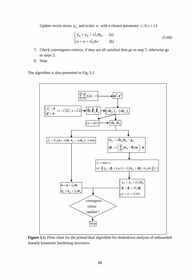
68

Update vector stress ikγ and scalar with a chosen parameter : 0 1

ˆ (a)

ˆ (b)

ik ik s ik

s

d

d

γ γ γ (5.60)

7. Check convergence criteria: if they are all satisfied then go to step 7, otherwise go

to steps 2.

8. Stop.

The algorithm is also presented in Fig. 5.1

Figure 5.1: Flow chart for the primal-dual algorithm for shakedown analysis of unbounded

linearly kinematic hardening structures.

Stop

0

1 1

1NG m

T

ik ik

i k

t e

0

0 1, ; 1,

ik

i

i NG k m

γ 0

β 0

0 0,u e

1 2, ik ikd de e

ˆ , mink P ik ikF d d u u e e

ˆ

ˆ

k

ik ik k ik

d

d

u u u

e e e

1

ˆ

ˆ

ik M ik ik

m

i ik i i

k

d c d

d c d d

γ D e g

β e B u h

1, 2ˆ ˆ ˆ,S f f

d , ikd du e

ˆ max

. . : 1

s

ik i ik ik i iks t d d d

γ β t γ β t

ˆ

ˆ

ˆ

ik ik s ik

i i s i

s

d

d

d

γ γ γ

β β β

convergence

criteria

satisfied ?

69

Chapter 6

Shakedown algorithm for elastic-plastic bounded

linearly kinematic hardening structures

6.1 Introduction

In this chapter, we solve problem (4.30) which has been established in chapter 4. Once

again, the penalty function method combined with the Lagrange multiplier method is used

to solve the constraint nonlinear optimization problem. Solution blkh

sd will be found by

upper the bound algorithm in section 6.2. This algorithm gives solutions for unbounded

kinematic hardening as presented in chapter 5 if 2u y , and it gives solutions for

structures made of perfectly plastic material if u y .

6.2 Upper bound algorithm

For sake of simplicity, we recall the new strain vector ike , the new fictitious elastic stress

vector ikt , and the new deformation matrix ˆiB as presented in Eqs. (5.1), (5.2) and (5.3) in

chapter 5. Then the nonlinear programming problem (4.30) of the shakedown limit load

factor becomes

223

1 1

2

1 1 1

1

min

(a)

s.t.:

ˆ 1,

ik

m NGT

blkh y ik ik

k i

NG m mu y T

ik ik

i k ky

m

ik i

k

i NG

ee e

e e

e B u

1 1

(b)

1 1, 1, (c)

3

1 (d)

M ik

m NGT

ik ik

k i

i NG k m

D e 0

e t

(6.1)

By writing the penalty function for the compatibility condition (6.1b) and the

incompressibility condition (6.1c), we obtain

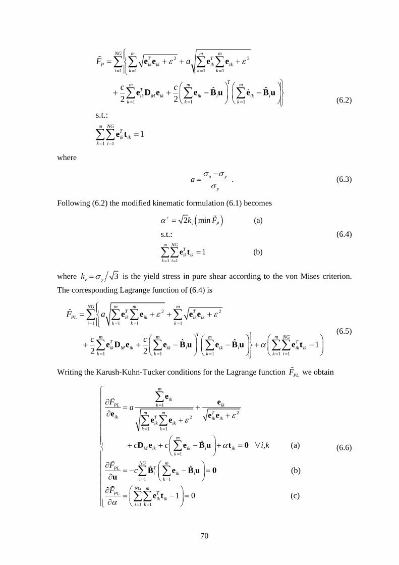
70

2 2

1 1 1 1

1 1 1

1 1

ˆ ˆ 2 2

s.t.:

1

NG m m mT T

P ik ik ik ik

i k k k

Tm m m

T

ik M ik ik i ik i

k k k

m NGT

ik ik

k i

F a

c c

e e e e

e D e e B u e B u

e t

(6.2)

where

u y

y

a

. (6.3)

Following (6.2) the modified kinematic formulation (6.1) becomes

1 1

2 min (a)

s.t.:

1 (b)

v P

m NGT

ik ik

k i

k F

e t

(6.4)

where 3v yk is the yield stress in pure shear according to the von Mises criterion.

The corresponding Lagrange function of (6.4) is

2 2

1 1 1 1

1 1 1 1 1

ˆ ˆ 12 2

NG m m mT T

PL ik ik ik ik

i k k k

Tm m m m NG

T T

ik M ik ik i ik i ik ik

k k k k i

F a

c c

e e e e

e D e e B u e B u e t

(6.5)

Writing the Karush-Kuhn-Tucker conditions for the Lagrange function PLF we obtain

1

22

1 1

1

1 1

ˆ (a)

ˆ ˆ (b)

m

ik

PL k ik

m m Tik T ik ik

ik ik

k k

m

M ik ik i ik

k

NG mTPLi ik i

i k

Fa

c c i,k

Fc

ee

e e ee e

D e e B u t 0

B e B u 0u

1 1

1 0 (c)NG m

TPLik ik

i k

F

e t

(6.6)

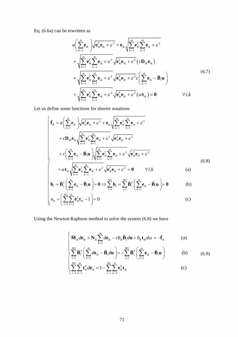
71

Eq. (6.6a) can be rewritten as

2 2

1 1 1

2 2

1 1

2 2

1 1 1

2 2

1 1

ˆ

m m mT T

ik ik ik ik ik ik

k k k

m mT T

ik ik ik ik M ik

k k

m m mT T

ik ik ik ik ik i

k k k

m mT T

ik ik ik ik ik

k k

a

c

c

e e e e e e

e e e e D e

e e e e e B u

e e e e t 0 i,k

(6.7)

Let us define some functions for shorter notations

2 2

1 1 1

2 2

1 1

2 2

1 1 1

2

1 1

ˆ

m m mT T

ik ik ik ik ik ik ik

k k k

m mT T

M ik ik ik ik ik

k k

m m mT T

ik i ik ik ik ik

k k k

m mT T

ik ik ik ik i

k k

a

c

c

f e e e e e e

D e e e e e

e B u e e e e

t e e e e2

1 1 1 1

1 1

(a)

ˆ ˆ ˆ ˆ (b)

1 0

k

m NG NG mT T

i i ik i i i ik i

k i i k

NG mT

ik ik ik

i k

i,k

n

0

h B e B u 0 h B e B u 0

e t (c)

(6.8)

Using the Newton-Raphson method to solve the system (6.8) we have

1

1 1 1 1

1 1

ˆ (a)

ˆ ˆ ˆ ˆ (b)

1

m

ik ik ik ik ik i ik ik ik

k

NG m NG mT T

i ik i i ik i

i k i k

NG mT T

ik ik ik ik

i k

d d cb d b d

d d

d

M e N e B u t f

B e B u B e B u

t e e t1 1

(c)NG m

i k

(6.9)

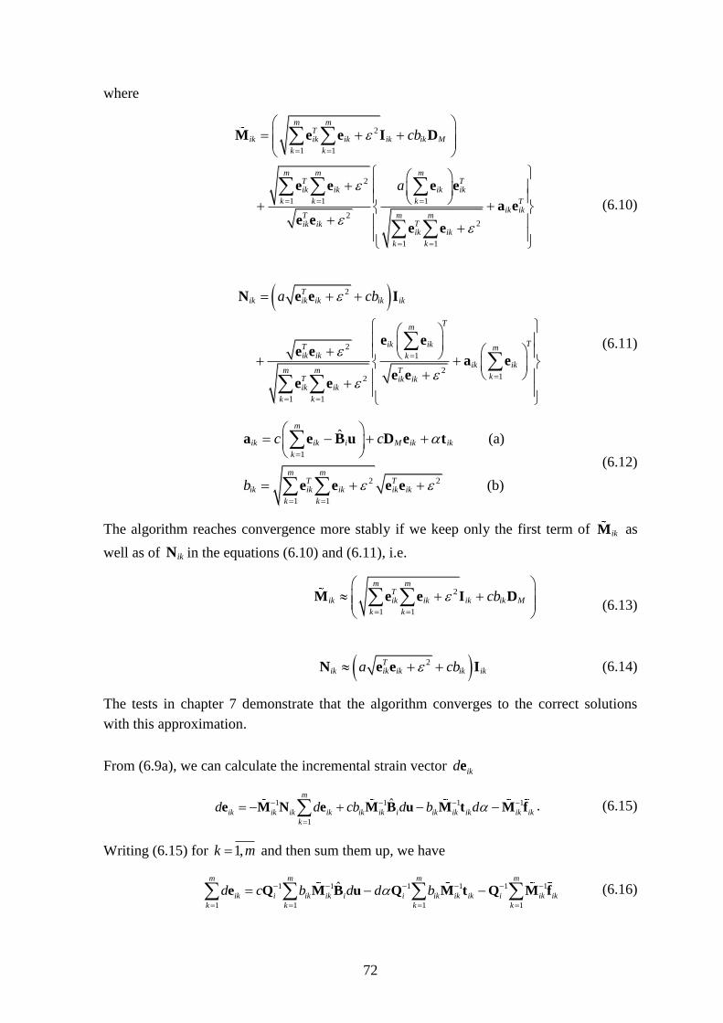
72

where

2

1 1

2

1 1 1

22

1 1

m mT

ik ik ik ik ik M

k k

m m mT Tik ik ik ik

k k k Tik ik

T m mTik ikik ik

k k

cb

a

M e e I D

e e e e

a ee e

e e

(6.10)

2

21

212

1 1

Tik ik ik ik ik

Tm

Tik ikT mik ik k

ik ikm m T

kT ik ikik ik

k k

a cb

N e e I

e ee e

a ee e

e e

(6.11)

1

2 2

1 1

ˆ (a)

(b)

m

ik ik i M ik ik

k

m mT T

ik ik ik ik ik

k k

c c

b

a e B u D e t

e e e e

(6.12)

The algorithm reaches convergence more stably if we keep only the first term of ikM as

well as of ikN in the equations (6.10) and (6.11), i.e.

2

1 1

m mT

ik ik ik ik ik M

k k

cb

M e e I D

(6.13)

2Tik ik ik ik ika cb N e e I (6.14)

The tests in chapter 7 demonstrate that the algorithm converges to the correct solutions

with this approximation.

From (6.9a), we can calculate the incremental strain vector ikde

1 1 1 1

1

ˆm

ik ik ik ik ik ik i ik ik ik ik ik

k

d d cb d b d

e M N e M B u M t M f . (6.15)

Writing (6.15) for 1,k m and then sum them up, we have

1 1 1 1 1 1

1 1 1 1

ˆm m m m

ik i ik ik i i ik ik ik i ik ik

k k k k

d c b d d b

e Q M B u Q M t Q M f (6.16)

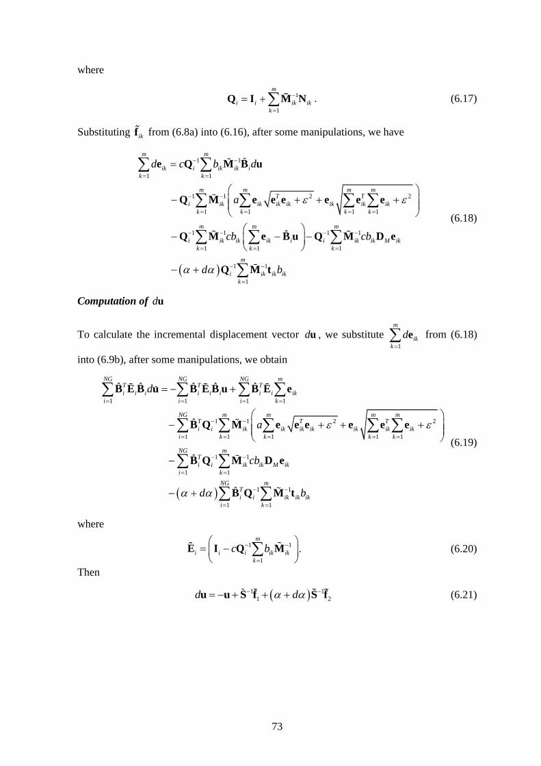
73

where

1

1

m

i i ik ik

k

Q I M N . (6.17)

Substituting ikf from (6.8a) into (6.16), after some manipulations, we have

1 1

1 1

1 1 2 2

1 1 1 1

1 1 1 1

1 1 1

ˆ

ˆ

m m

ik i ik ik i

k k

m m m mT T

i ik ik ik ik ik ik ik

k k k k

m m m

i ik ik ik i i ik ik M ik

k k k

d c b d

a

cb cb

e Q M B u

Q M e e e e e e

Q M e B u Q M D e

1 1

1

m

i ik ik ik

k

d b

Q M t

(6.18)

Computation of du

To calculate the incremental displacement vector du , we substitute 1

m

ik

k

d

e from (6.18)

into (6.9b), after some manipulations, we obtain

1 1 1 1

1 1 2 2

1 1 1 1 1

1

1

ˆ ˆ ˆ ˆ ˆ

ˆ

ˆ

NG NG NG mT T T

i i i i i i i i ik

i i i k

NG m m m mT T T

i i ik ik ik ik ik ik ik

i k k k k

NGT

i i

i

d

a

B E B u B E B u B E e

B Q M e e e e e e

B Q M

1

1

1 1

1 1

ˆ

m

ik ik M ik

k

NG mT

i i ik ik ik

i k

cb

d b

D e

B Q M t

(6.19)

where

1 1

1

m

i i i ik ik

k

c b

E I Q M . (6.20)

Then

1 1

1 2d d u u S f S f (6.21)

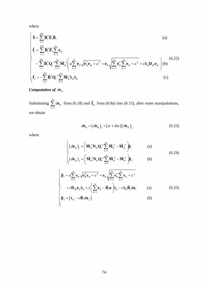
74

where

1

1

1 1

1 1 2

1 1 1

ˆ ˆ (a)

ˆ

ˆ

NGT

i i i

i

NG mT

i i ik

i k

NG mT T T

i i ik ik ik ik ik ik

i k k

a

S B E B

f B E e

B Q M e e e e e2

1 1

1 1

2

1 1

(b)

ˆ (c)

m m m

ik ik M ik

k k

NG mT

i i ik ik ik

i k

cb

b

e D e

f B Q M t

(6.22)

Computation of ikde

Substituting 1

m

ik

k

d

e from (6.18) and ikf from (6.8a) into (6.15), after some manipulations,

we obtain


where

1 1 1 1

111

1 1 1 1

221

(a)

(b)

m

ik ik ik i ik ik

k

m

ik ik ik i ik ik

k

d

d

e M N Q M M β

e M N Q M M β

(6.24)

2 2

1

1 1 1

1

1

2 2

ˆ ˆ (a)

ˆ (b)

m m mT T

ik ik ik ik ik ik

k k k

m

M ik ik ik i ik ik i

k

ik i

a

c b c b cb d

c d

β e e e e e e

D e e B u B u

β t B u

(6.25)

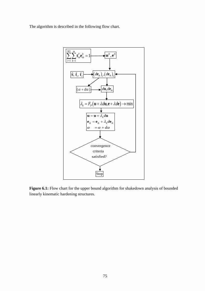
75

The algorithm is described in the following flow chart.

Figure 6.1: Flow chart for the upper bound algorithm for shakedown analysis of bounded

linearly kinematic hardening structures.

Stop

0 0,u e

1 2,ik ikd de e

1 2, , S f f

d

convergence

criteria

satisfied?

, ikd du e

0

1 1

1NG m

T

ik ik

i k

t e

, mink PF d d u u e e

k

ik ik k ik

d

d

d

u u u

e e e

77

Chapter 7

Validations and parametric studies

In this chapter, firstly we validate our theory and algorithms by analysing many examples,

which are available in literature. For limit analysis, the results are verified by

lim lim

blkh pp

u y , where u y . For shakedown analysis, the results are verified by

, for perfectly plastic structures

2 , for bounded and unbounded kinematic hardening

blkh pp

sd sd

pp blkh ppusd sd sd el

y

Secondly, we do the parametric study, where the penalty parameter c and the value

of are varied to see their influence on the solution, and to confirm their interval value for

stable results.

Test cases cover 2D and 3D finite elements, thermal load to mechanical loads, and

from simple to complicated structures and loadings.

7.1 Structure 1: Thin plate under tension and temperature

Problem definitions

This problem has investigated in Heitzer, Staat (2003), using a numerical approach

based on the lower bound shakedown theorem.

Geometry: The square plate has the dimensions: 2400 400 mmB L , supported at

the top and bottom sides, see Fig. 7.1.1.

Material: Young’s modulus: 5 22.1 10 N/mmE , yield stress: 2160 N/mmy ,

hardening effect (ultimate strength): 1.5u y for bounded hardening,

and 2u y for unbounded hardening, Poisson’s ratio: 0.3 ,

coefficient of thermal expansion: 5 110 Kt .

Loads: uniform distributed tension N/mmp applied on the lateral sides, and

uniform distributed temperature °CT on the plate, these loads vary in the

domain: 00,p p , 00,T T , where 0p and 0T is the elastic analytical

solution for pure tension and pure temperature, respectively, see details in

Heitzer, Staat (2003)

02

1

1yp

and 0

1y

t

TE

. (7.1.1)

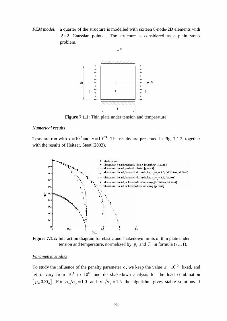
78

FEM model: a quarter of the structure is modelled with sixteen 8-node-2D elements with

2 2 Gaussian points . The structure is considered as a plain stress

problem.

Figure 7.1.1: Thin plate under tension and temperature.

Numerical results

Tests are run with 1010c and

2410 . The results are presented in Fig. 7.1.2, together

with the results of Heitzer, Staat (2003).

Figure 7.1.2: Interaction diagram for elastic and shakedown limits of thin plate under

tension and temperature, normalized by 0p and 0T in formula (7.1.1).

Parametric studies

To study the influence of the penalty parameter c , we keep the value 2410 fixed, and

let c vary from 410 to

1710 and do shakedown analysis for the load combination

0 0,0.3p T . For 1.0u y and 1.5u y the algorithm gives stable solutions if

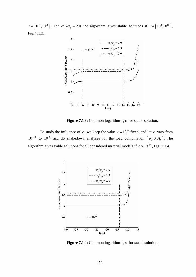
79

6 1410 ,10c . For 2.0u y the algorithm gives stable solutions if 4 1510 ,10c ,

Fig. 7.1.3.

Figure 7.1.3: Common logarithm lg c for stable solution.

To study the influence of , we keep the value 1010c fixed, and let vary from

4010 to

910 and do shakedown analyses for the load combination 0 0,0.3p T . The

algorithm gives stable solutions for all considered material models if 1410 , Fig. 7.1.4.

Figure 7.1.4: Common logarithm lg for stable solution.

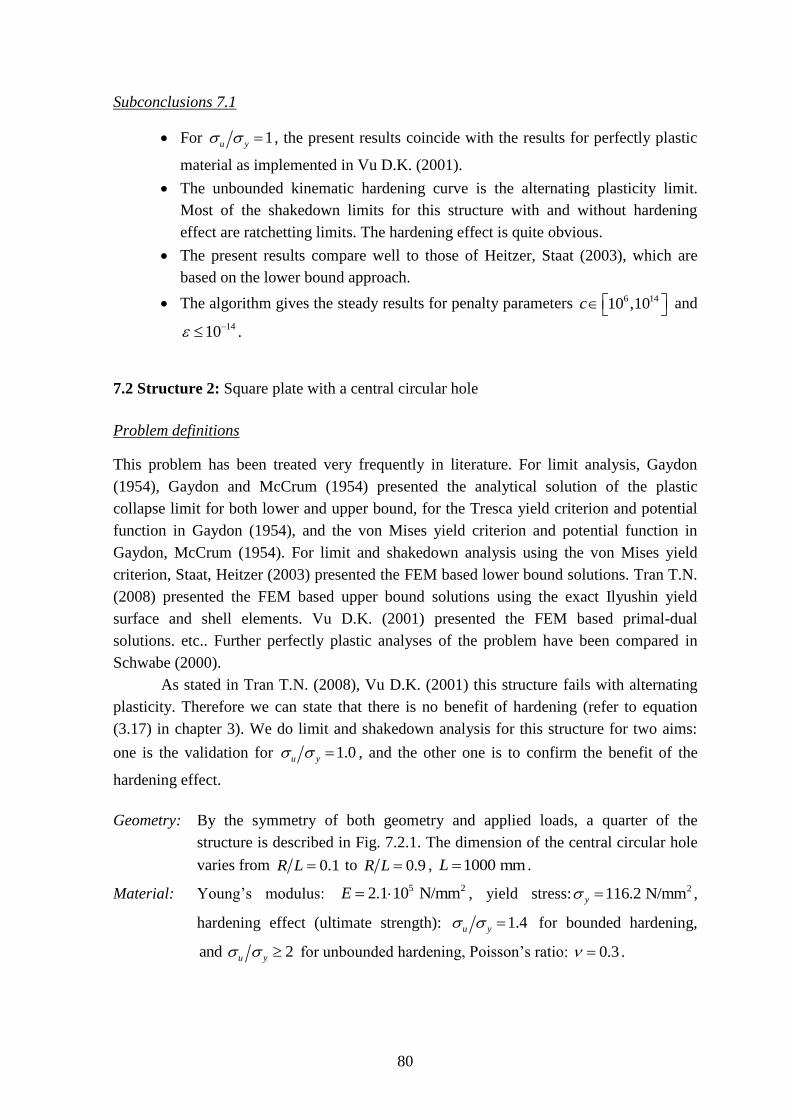
80

Subconclusions 7.1

For 1u y , the present results coincide with the results for perfectly plastic

material as implemented in Vu D.K. (2001).

The unbounded kinematic hardening curve is the alternating plasticity limit.

Most of the shakedown limits for this structure with and without hardening

effect are ratchetting limits. The hardening effect is quite obvious.

The present results compare well to those of Heitzer, Staat (2003), which are

based on the lower bound approach.

The algorithm gives the steady results for penalty parameters 6 1410 ,10c and

1410 .

7.2 Structure 2: Square plate with a central circular hole

Problem definitions

This problem has been treated very frequently in literature. For limit analysis, Gaydon

(1954), Gaydon and McCrum (1954) presented the analytical solution of the plastic

collapse limit for both lower and upper bound, for the Tresca yield criterion and potential

function in Gaydon (1954), and the von Mises yield criterion and potential function in

Gaydon, McCrum (1954). For limit and shakedown analysis using the von Mises yield

criterion, Staat, Heitzer (2003) presented the FEM based lower bound solutions. Tran T.N.

(2008) presented the FEM based upper bound solutions using the exact Ilyushin yield

surface and shell elements. Vu D.K. (2001) presented the FEM based primal-dual

solutions. etc.. Further perfectly plastic analyses of the problem have been compared in

Schwabe (2000).

As stated in Tran T.N. (2008), Vu D.K. (2001) this structure fails with alternating

plasticity. Therefore we can state that there is no benefit of hardening (refer to equation

(3.17) in chapter 3). We do limit and shakedown analysis for this structure for two aims:

one is the validation for 1.0u y , and the other one is to confirm the benefit of the

hardening effect.

Geometry: By the symmetry of both geometry and applied loads, a quarter of the

structure is described in Fig. 7.2.1. The dimension of the central circular hole

varies from 0.1R L to 0.9R L , 1000 mmL .

Material: Young’s modulus: 5 22.1 10 N/mmE , yield stress: 2116.2 N/mmy ,


and 2u y for unbounded hardening, Poisson’s ratio: 0.3 .

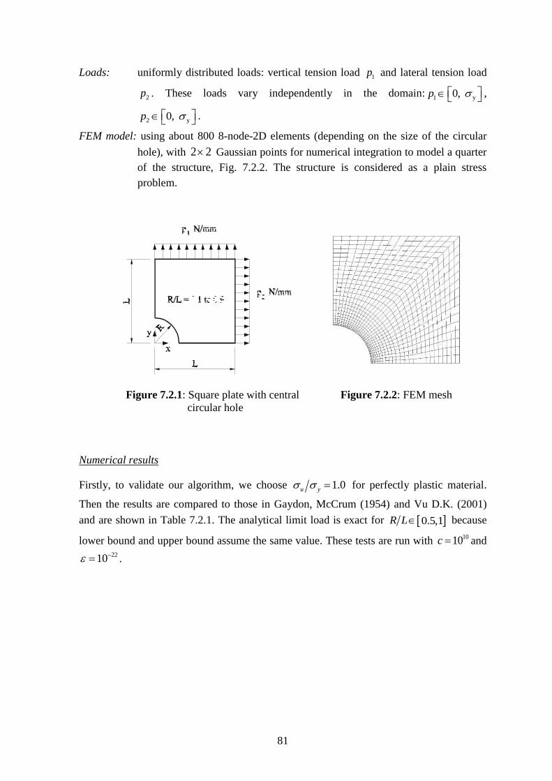
81

Loads: uniformly distributed loads: vertical tension load 1p and lateral tension load

2p . These loads vary independently in the domain:1 y0, p ,

2 y0, p .

FEM model: using about 800 8-node-2D elements (depending on the size of the circular

hole), with 2 2 Gaussian points for numerical integration to model a quarter

of the structure, Fig. 7.2.2. The structure is considered as a plain stress

problem.

Figure 7.2.1: Square plate with central

circular hole

Figure 7.2.2: FEM mesh

Numerical results

Firstly, to validate our algorithm, we choose 1.0u y for perfectly plastic material.

Then the results are compared to those in Gaydon, McCrum (1954) and Vu D.K. (2001)

and are shown in Table 7.2.1. The analytical limit load is exact for 0.5,1R L because

lower bound and upper bound assume the same value. These tests are run with 1010c and

2210 .

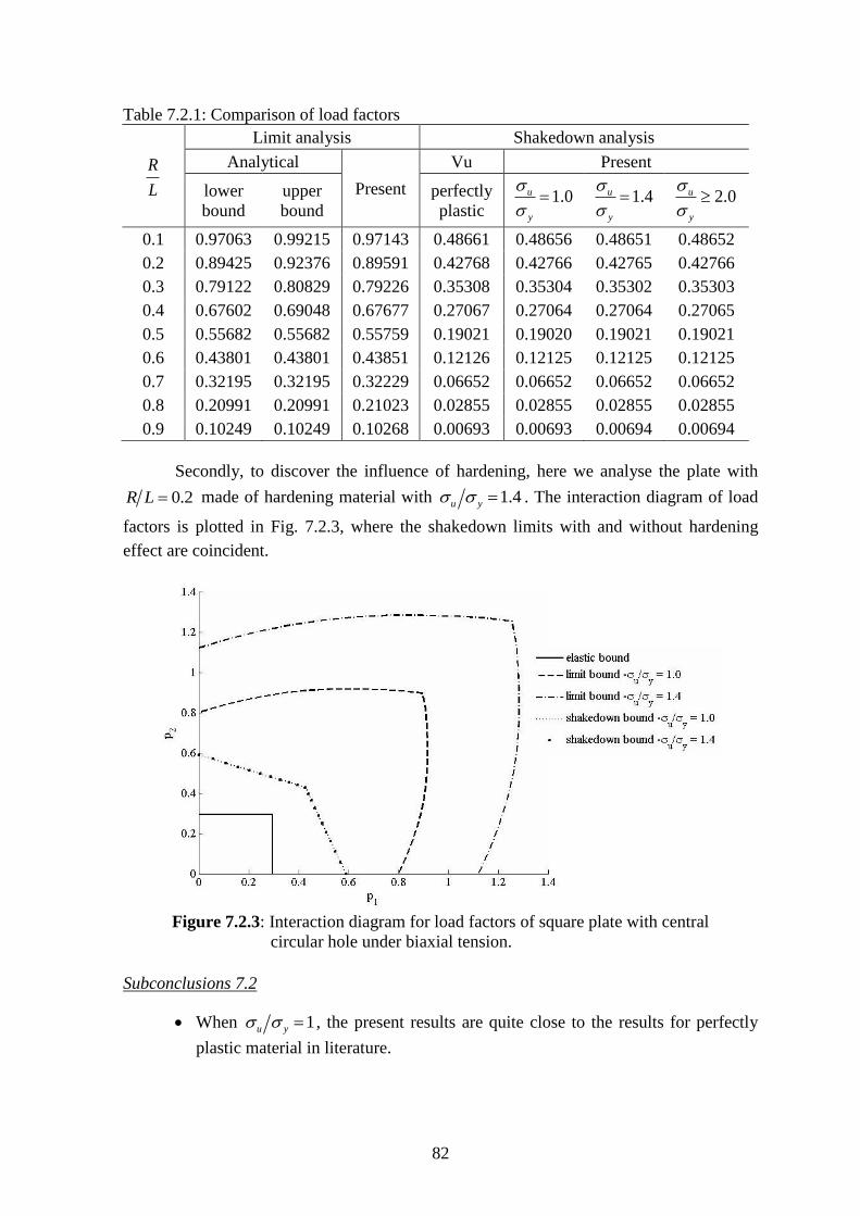
82

Table 7.2.1: Comparison of load factors

R

L

Limit analysis Shakedown analysis

Analytical

Present

Vu Present

lower

bound

upper

bound

perfectly

plastic 1.0u

y

1.4u

y

2.0u

y

0.1 0.97063 0.99215 0.97143 0.48661 0.48656 0.48651 0.48652

0.2 0.89425 0.92376 0.89591 0.42768 0.42766 0.42765 0.42766

0.3 0.79122 0.80829 0.79226 0.35308 0.35304 0.35302 0.35303

0.4 0.67602 0.69048 0.67677 0.27067 0.27064 0.27064 0.27065

0.5 0.55682 0.55682 0.55759 0.19021 0.19020 0.19021 0.19021

0.6 0.43801 0.43801 0.43851 0.12126 0.12125 0.12125 0.12125

0.7 0.32195 0.32195 0.32229 0.06652 0.06652 0.06652 0.06652

0.8 0.20991 0.20991 0.21023 0.02855 0.02855 0.02855 0.02855

0.9 0.10249 0.10249 0.10268 0.00693 0.00693 0.00694 0.00694

Secondly, to discover the influence of hardening, here we analyse the plate with

0.2R L made of hardening material with 1.4u y . The interaction diagram of load

factors is plotted in Fig. 7.2.3, where the shakedown limits with and without hardening

effect are coincident.

Figure 7.2.3: Interaction diagram for load factors of square plate with central

circular hole under biaxial tension.

Subconclusions 7.2

When 1u y , the present results are quite close to the results for perfectly

plastic material in literature.

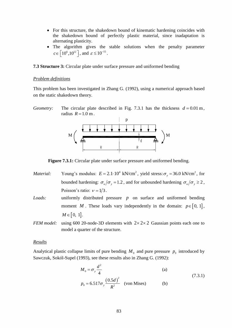
83

For this structure, the shakedown bound of kinematic hardening coincides with

the shakedown bound of perfectly plastic material, since inadaptation is

alternating plasticity.

The algorithm gives the stable solutions when the penalty parameter 6 1210 ,10c , and

1510 .

7.3 Structure 3: Circular plate under surface pressure and uniformed bending

Problem definitions

This problem has been investigated in Zhang G. (1992), using a numerical approach based

on the static shakedown theory.

Geometry: The circular plate described in Fig. 7.3.1 has the thickness 0.01 md ,

radius 1.0 mR .

p

MM

Figure 7.3.1: Circular plate under surface pressure and uniformed bending.

Material: Young’s modulus: 4 22.1 10 kN/cmE , yield stress: 236.0 kN/cmy , for

bounded hardening: 1.2u y , and for unbounded hardening 2u y ,

Poisson’s ratio: 1 3 .

Loads: uniformly distributed pressure p on surface and uniformed bending

moment M . These loads vary independently in the domain: 0, 1p ,

0, 1M .

FEM model: using 600 20-node-3D elements with 2 2 2 Gaussian points each one to

model a quarter of the structure.

Results

Analytical plastic collapse limits of pure bending 0M and pure pressure 0p introduced by

Sawczuk, Sokól-Supel (1993), see these results also in Zhang G. (1992):

2

0

2

0 2

(a)4

0.56.517 (von Mises) (b)

y

y

dM

dp

R

(7.3.1)

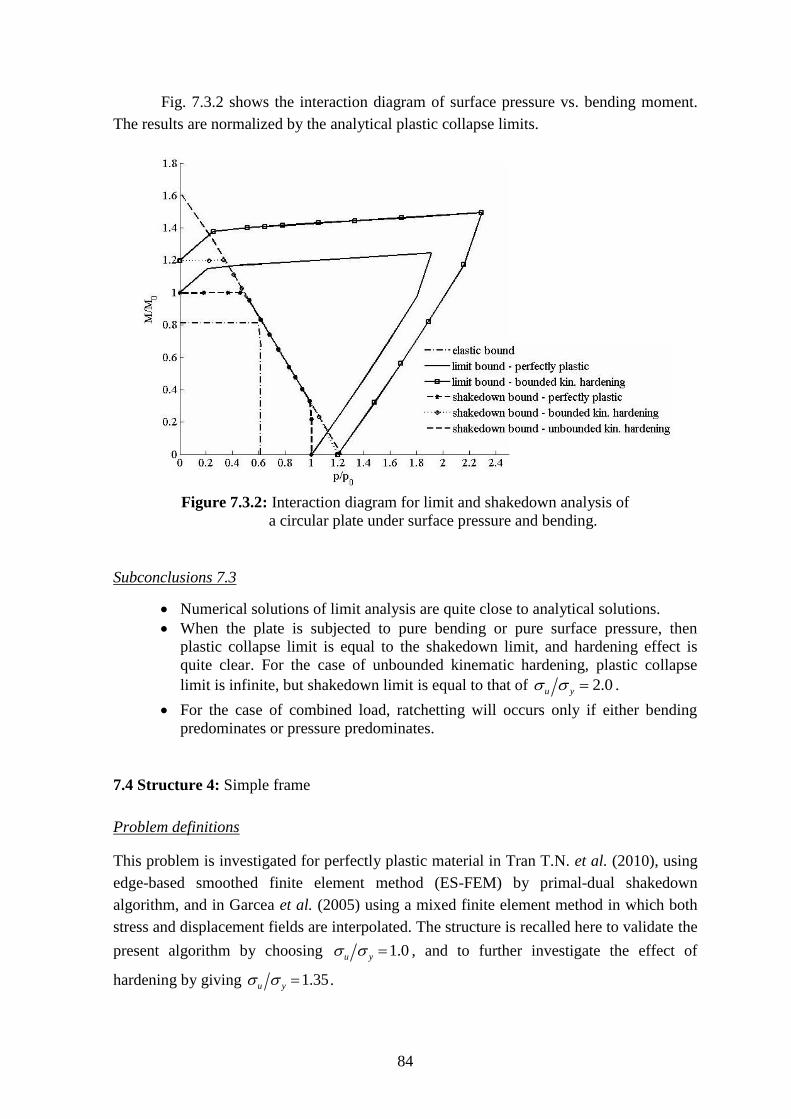
84

Fig. 7.3.2 shows the interaction diagram of surface pressure vs. bending moment.

The results are normalized by the analytical plastic collapse limits.

Figure 7.3.2: Interaction diagram for limit and shakedown analysis of

a circular plate under surface pressure and bending.

Subconclusions 7.3

Numerical solutions of limit analysis are quite close to analytical solutions.

When the plate is subjected to pure bending or pure surface pressure, then

plastic collapse limit is equal to the shakedown limit, and hardening effect is

quite clear. For the case of unbounded kinematic hardening, plastic collapse

limit is infinite, but shakedown limit is equal to that of 2.0u y .

For the case of combined load, ratchetting will occurs only if either bending

predominates or pressure predominates.

7.4 Structure 4: Simple frame

Problem definitions

This problem is investigated for perfectly plastic material in Tran T.N. et al. (2010), using

edge-based smoothed finite element method (ES-FEM) by primal-dual shakedown

algorithm, and in Garcea et al. (2005) using a mixed finite element method in which both

stress and displacement fields are interpolated. The structure is recalled here to validate the

present algorithm by choosing 1.0u y , and to further investigate the effect of

hardening by giving 1.35u y .

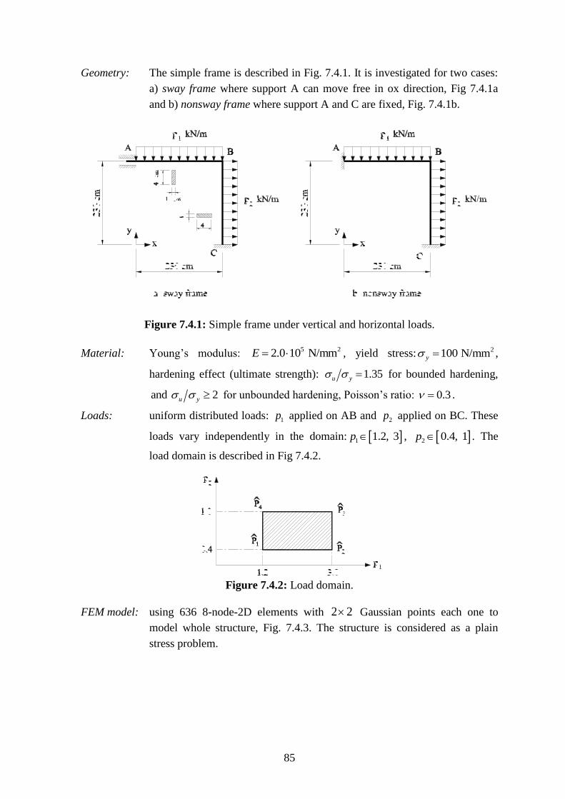
85

Geometry: The simple frame is described in Fig. 7.4.1. It is investigated for two cases:

a) sway frame where support A can move free in ox direction, Fig 7.4.1a

and b) nonsway frame where support A and C are fixed, Fig. 7.4.1b.

Figure 7.4.1: Simple frame under vertical and horizontal loads.



and 2u y for unbounded hardening, Poisson’s ratio: 0.3 .

Loads: uniform distributed loads: 1p applied on AB and 2p applied on BC. These

loads vary independently in the domain: 1 1.2, 3p , 2 0.4, 1p . The

load domain is described in Fig 7.4.2.

Figure 7.4.2: Load domain.

FEM model: using 636 8-node-2D elements with 2 2 Gaussian points each one to

model whole structure, Fig. 7.4.3. The structure is considered as a plain

stress problem.

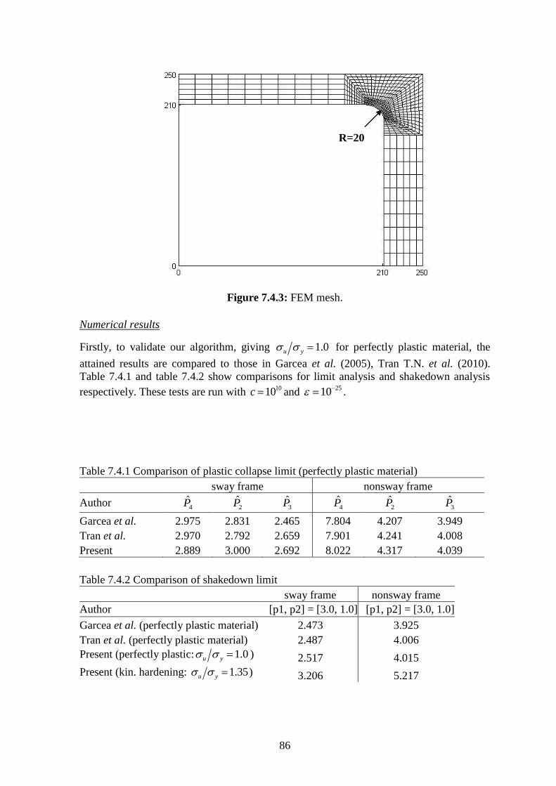
86

Figure 7.4.3: FEM mesh.

Numerical results

Firstly, to validate our algorithm, giving 1.0u y for perfectly plastic material, the

attained results are compared to those in Garcea et al. (2005), Tran T.N. et al. (2010).

Table 7.4.1 and table 7.4.2 show comparisons for limit analysis and shakedown analysis

respectively. These tests are run with 1010c and

2510 .

Table 7.4.1 Comparison of plastic collapse limit (perfectly plastic material)

sway frame nonsway frame

Author 4P̂ 2P̂ 3P̂ 4P̂ 2P̂ 3P̂

Garcea et al. 2.975 2.831 2.465 7.804 4.207 3.949

Tran et al. 2.970 2.792 2.659 7.901 4.241 4.008

Present 2.889 3.000 2.692 8.022 4.317 4.039

Table 7.4.2 Comparison of shakedown limit

sway frame nonsway frame

Author [p1, p2] = [3.0, 1.0] [p1, p2] = [3.0, 1.0]

Garcea et al. (perfectly plastic material) 2.473 3.925

Tran et al. (perfectly plastic material) 2.487 4.006

Present (perfectly plastic: 1.0u y ) 2.517 4.015

Present (kin. hardening: 1.35u y ) 3.206 5.217

R=20

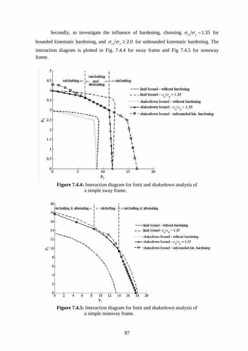
87

Secondly, to investigate the influence of hardening, choosing 1.35u y for

bounded kinematic hardening, and 2.0u y for unbounded kinematic hardening. The

interaction diagram is plotted in Fig. 7.4.4 for sway frame and Fig 7.4.5 for nonsway

frame.


a simple sway frame.


a simple nonsway frame.

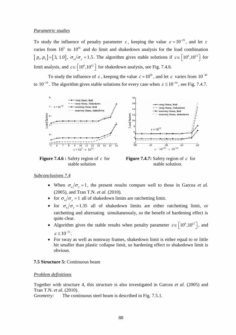
88

Parametric studies

To study the influence of penalty parameter c , keeping the value 2510 , and let c

varies from 510 to

1610 and do limit and shakedown analysis for the load combination

1 2, 3, 1.0p p , 1.5u y . The algorithm gives stable solutions if 6 1310 ,10c for

limit analysis, and 6 1210 ,10c for shakedown analysis, see Fig. 7.4.6.

To study the influence of , keeping the value 1010c , and let varies from

3010

to 1010

. The algorithm gives stable solutions for every case when 1410 , see Fig. 7.4.7.

Figure 7.4.6 : Safety region of c for

stable solution

Figure 7.4.7: Safety region of for

stable solution.

Subconclusions 7.4

When 1u y , the present results compare well to those in Garcea et al.

(2005), and Tran T.N. et al. (2010).

for 1u y all of shakedown limits are ratchetting limit.

for 1.35u y all of shakedown limits are either ratchetting limit, or

ratchetting and alternating simultaneously, so the benefit of hardening effect is

quite clear.

Algorithm gives the stable results when penalty parameter 6 1210 ,10c , and

1510 .

For sway as well as nonsway frames, shakedown limit is either equal to or little

bit smaller than plastic collapse limit, so hardening effect to shakedown limit is

obvious.

7.5 Structure 5: Continuous beam

Problem definitions

Together with structure 4, this structure is also investigated in Garcea et al. (2005) and

Tran T.N. et al. (2010).

Geometry: The continuous steel beam is described in Fig. 7.5.1.

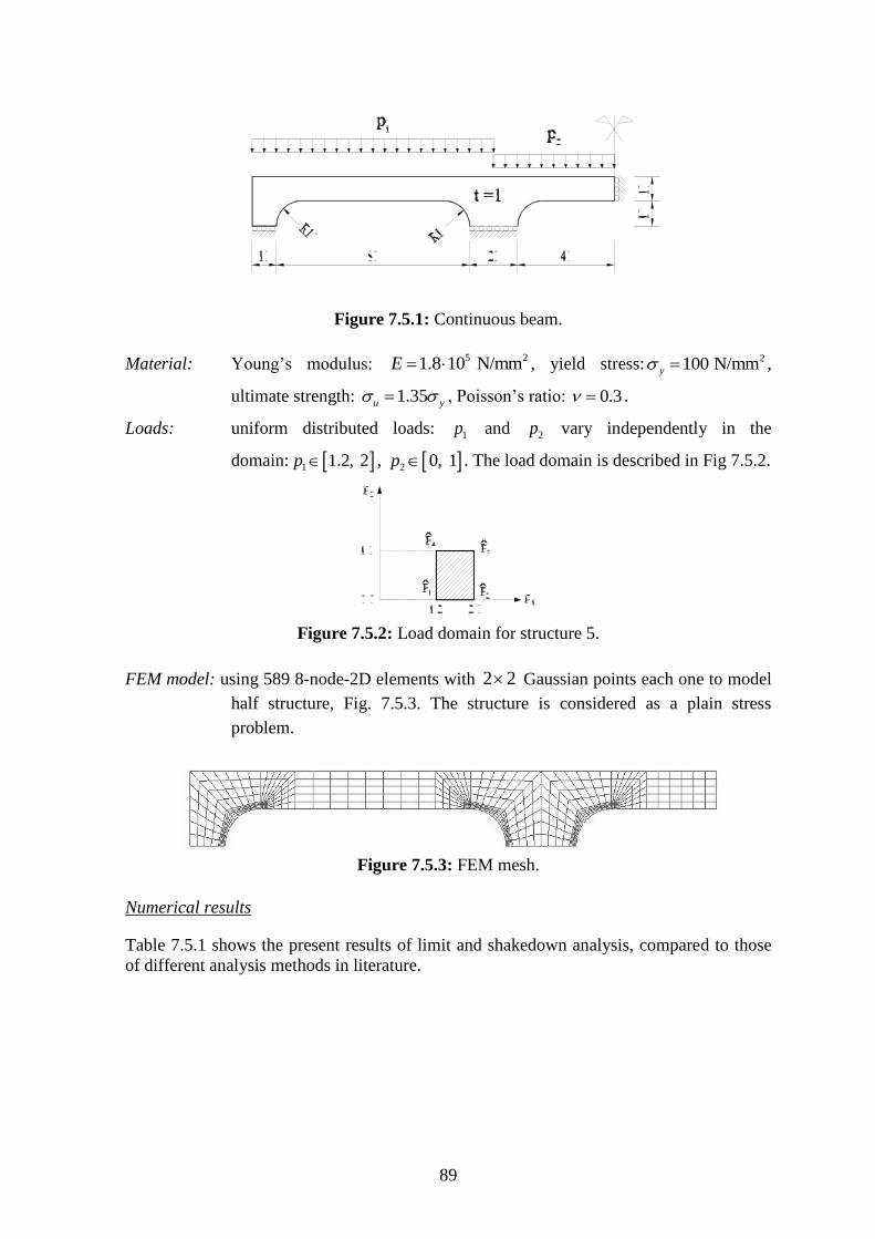
89

Figure 7.5.1: Continuous beam.


ultimate strength: 1.35u y , Poisson’s ratio: 0.3 .

Loads: uniform distributed loads: 1p and 2p vary independently in the

domain: 1 1.2, 2p , 2 0, 1p . The load domain is described in Fig 7.5.2.

Figure 7.5.2: Load domain for structure 5.

FEM model: using 589 8-node-2D elements with 2 2 Gaussian points each one to model

half structure, Fig. 7.5.3. The structure is considered as a plain stress

problem.


Numerical results

Table 7.5.1 shows the present results of limit and shakedown analysis, compared to those

of different analysis methods in literature.

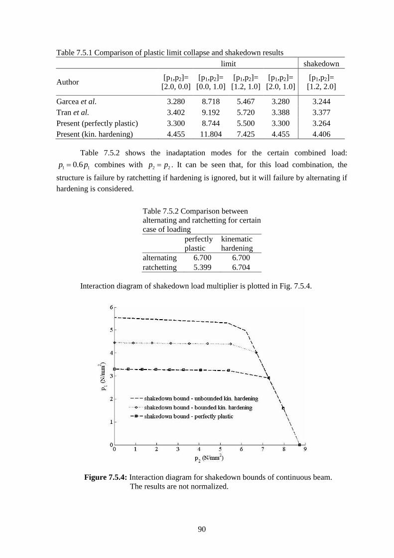
90

Table 7.5.1 Comparison of plastic limit collapse and shakedown results

limit shakedown

Author [p1,p2]=

[2.0, 0.0]

[p1,p2]=

[0.0, 1.0]

[p1,p2]=

[1.2, 1.0]

[p1,p2]=

[2.0, 1.0]

[p1,p2]=

[1.2, 2.0]

Garcea et al. 3.280 8.718 5.467 3.280 3.244

Tran et al. 3.402 9.192 5.720 3.388 3.377

Present (perfectly plastic) 3.300 8.744 5.500 3.300 3.264

Present (kin. hardening) 4.455 11.804 7.425 4.455 4.406

Table 7.5.2 shows the inadaptation modes for the certain combined load:

1 10.6p p combines with 2 2p p . It can be seen that, for this load combination, the

structure is failure by ratchetting if hardening is ignored, but it will failure by alternating if

hardening is considered.

Table 7.5.2 Comparison between

alternating and ratchetting for certain

case of loading

perfectly

plastic

kinematic

hardening

alternating 6.700 6.700

ratchetting 5.399 6.704

Interaction diagram of shakedown load multiplier is plotted in Fig. 7.5.4.

Figure 7.5.4: Interaction diagram for shakedown bounds of continuous beam.

The results are not normalized.

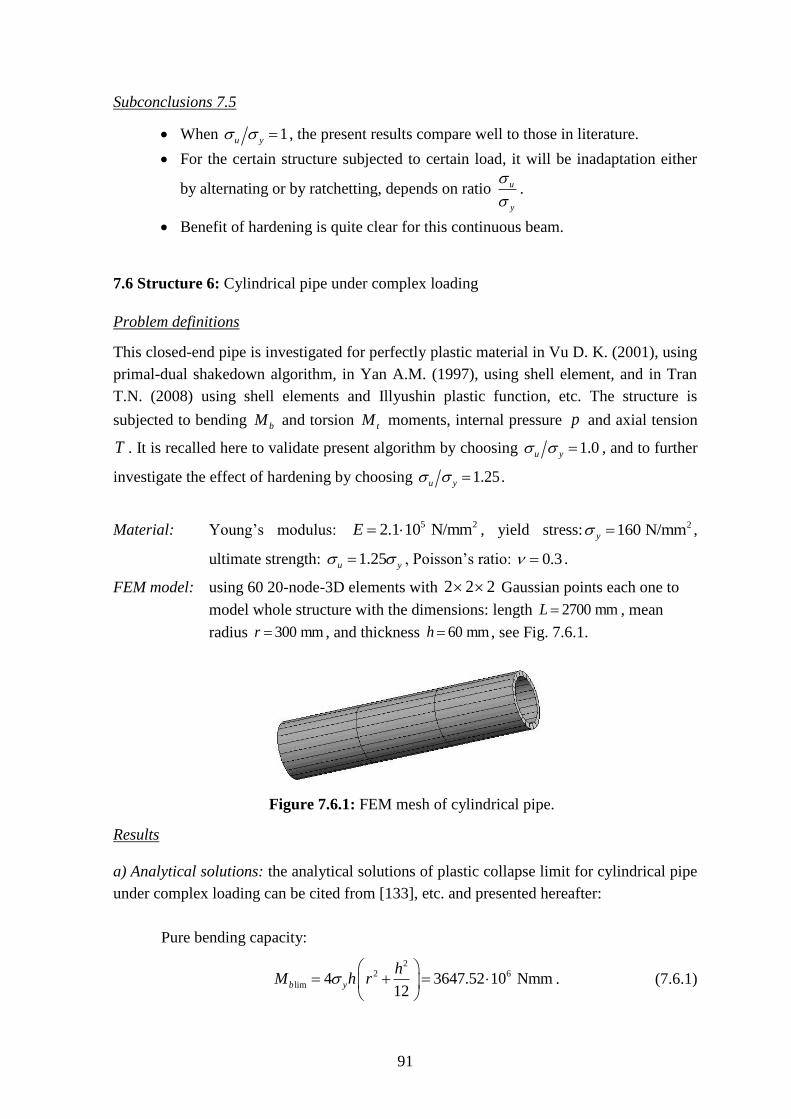
91

Subconclusions 7.5

When 1u y , the present results compare well to those in literature.

For the certain structure subjected to certain load, it will be inadaptation either

by alternating or by ratchetting, depends on ratio u

y

.

Benefit of hardening is quite clear for this continuous beam.

7.6 Structure 6: Cylindrical pipe under complex loading

Problem definitions

This closed-end pipe is investigated for perfectly plastic material in Vu D. K. (2001), using

primal-dual shakedown algorithm, in Yan A.M. (1997), using shell element, and in Tran

T.N. (2008) using shell elements and Illyushin plastic function, etc. The structure is

subjected to bending bM and torsion tM moments, internal pressure p and axial tension

T . It is recalled here to validate present algorithm by choosing 1.0u y , and to further

investigate the effect of hardening by choosing 1.25u y .



FEM model: using 60 20-node-3D elements with 2 2 2 Gaussian points each one to

model whole structure with the dimensions: length 2700 mmL , mean

radius 300 mmr , and thickness 60 mmh , see Fig. 7.6.1.

Figure 7.6.1: FEM mesh of cylindrical pipe.

Results

a) Analytical solutions: the analytical solutions of plastic collapse limit for cylindrical pipe

under complex loading can be cited from [133], etc. and presented hereafter:

Pure bending capacity:

22 6

lim 4 3647.52 10 Nmm12

b y

hM h r

. (7.6.1)

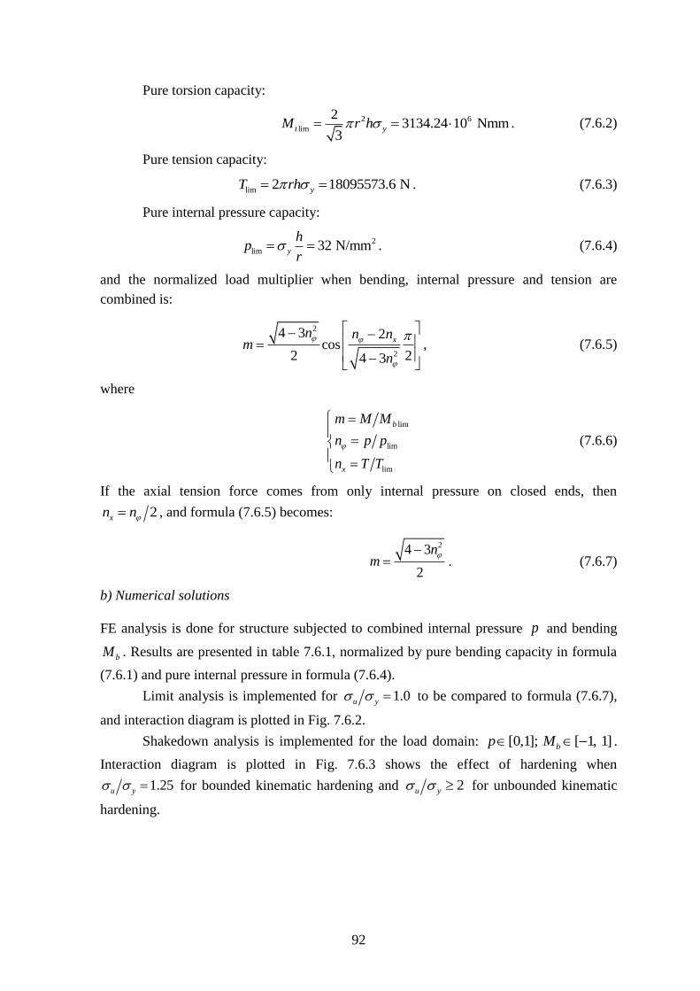
92

Pure torsion capacity:

2 6

lim

23134.24 10 Nmm

3t yM r h . (7.6.2)

Pure tension capacity:

lim 2 18095573.6 NyT rh . (7.6.3)

Pure internal pressure capacity:

2

lim 32 N/mmy

hp

r . (7.6.4)

and the normalized load multiplier when bending, internal pressure and tension are

combined is:

2

2

4 3 2cos

2 24 3

xn n n

mn

, (7.6.5)

where

lim

lim

lim

b

x

m M M

n p p

n T T

(7.6.6)

If the axial tension force comes from only internal pressure on closed ends, then

2xn n , and formula (7.6.5) becomes:

24 3

2

nm

. (7.6.7)

b) Numerical solutions

FE analysis is done for structure subjected to combined internal pressure p and bending

bM . Results are presented in table 7.6.1, normalized by pure bending capacity in formula

(7.6.1) and pure internal pressure in formula (7.6.4).

Limit analysis is implemented for 1.0u y to be compared to formula (7.6.7),

and interaction diagram is plotted in Fig. 7.6.2.

Shakedown analysis is implemented for the load domain: [0,1]; [ 1, 1]bp M .

Interaction diagram is plotted in Fig. 7.6.3 shows the effect of hardening when

1.25u y for bounded kinematic hardening and 2u y for unbounded kinematic

hardening.

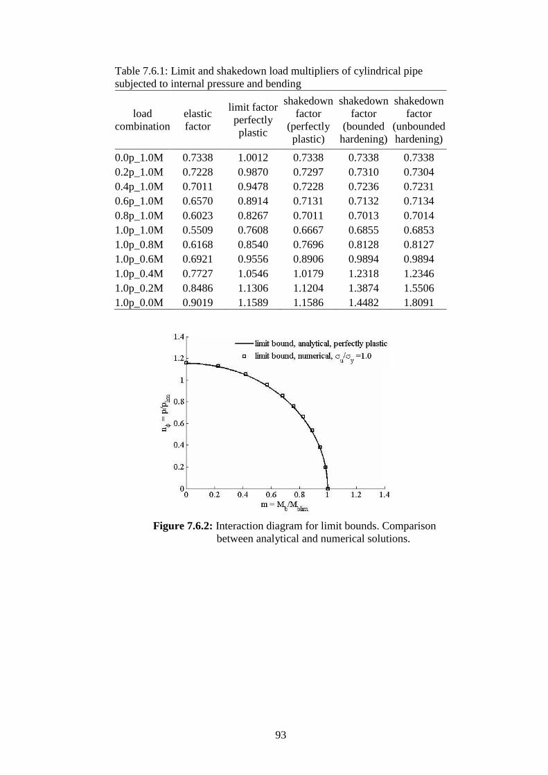
93

Table 7.6.1: Limit and shakedown load multipliers of cylindrical pipe

subjected to internal pressure and bending

load

combination

elastic

factor

limit factor

perfectly

plastic

shakedown

factor

(perfectly

plastic)

shakedown

factor

(bounded

hardening)

shakedown

factor

(unbounded

hardening)

0.0p_1.0M 0.7338 1.0012 0.7338 0.7338 0.7338

0.2p_1.0M 0.7228 0.9870 0.7297 0.7310 0.7304

0.4p_1.0M 0.7011 0.9478 0.7228 0.7236 0.7231

0.6p_1.0M 0.6570 0.8914 0.7131 0.7132 0.7134

0.8p_1.0M 0.6023 0.8267 0.7011 0.7013 0.7014

1.0p_1.0M 0.5509 0.7608 0.6667 0.6855 0.6853

1.0p_0.8M 0.6168 0.8540 0.7696 0.8128 0.8127

1.0p_0.6M 0.6921 0.9556 0.8906 0.9894 0.9894

1.0p_0.4M 0.7727 1.0546 1.0179 1.2318 1.2346

1.0p_0.2M 0.8486 1.1306 1.1204 1.3874 1.5506

1.0p_0.0M 0.9019 1.1589 1.1586 1.4482 1.8091

Figure 7.6.2: Interaction diagram for limit bounds. Comparison

between analytical and numerical solutions.

94

Figure 7.6.3: Interaction diagram for elastic and shakedown bounds,

normalized by pure plastic collapse limits, limbM and limp .

Subconclusions 7.6

The present results of limit analysis for 1u y compare well to analytical

solutions.

The hardening effect increases the pressure capacity clearly if the moment is less

than lim0.5 bM .

The shakedown bound of unbounded hardening structure cannot exceed two

times of elastic bound.

7.7 Structure 7: Grooved rectangle plate under tension and bending

Problem definitions:

This structure made of perfectly plastic material has been analysed by many authors. Limit

analysis for pure tension load 0, 0N Mp p has been done by Prager and Hodge

(1951), Casiaro and Cascini (1982) and Yan A.M. (1997). For combined tension and

bending 0, 0N Mp p , limit and shakedown analyses have been done by Heitzer

(1999), Vu D.K. (2001) and Tran T.N. (2008). Their results are close together, so it is

sufficient to compare the present results to one out of those.

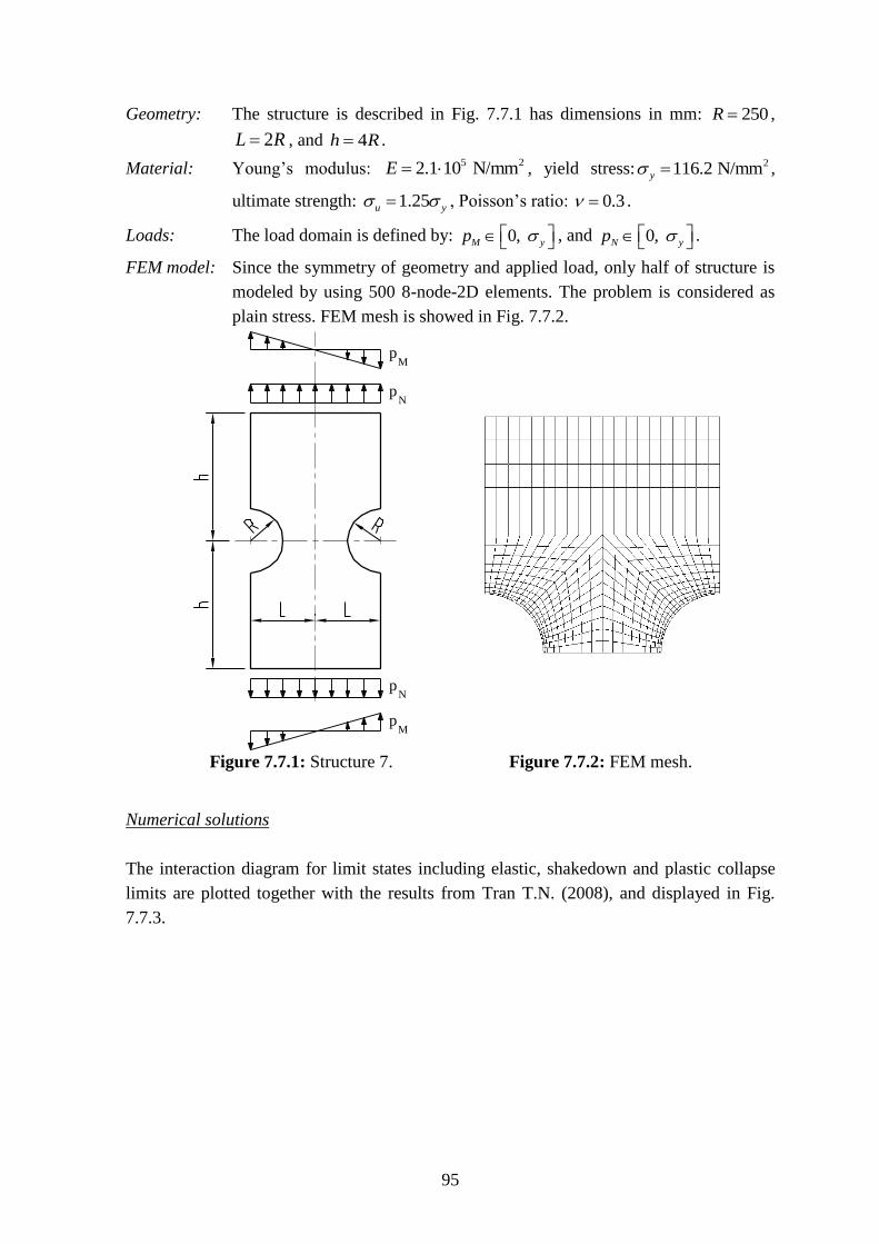
95

Geometry: The structure is described in Fig. 7.7.1 has dimensions in mm: 250R ,

2L R , and 4h R .

Material: Young’s modulus: 5 22.1 10 N/mmE , yield stress: 2116.2 N/mmy ,


Loads: The load domain is defined by: 0, M yp , and 0, N yp .

FEM model: Since the symmetry of geometry and applied load, only half of structure is

modeled by using 500 8-node-2D elements. The problem is considered as

plain stress. FEM mesh is showed in Fig. 7.7.2.

pN

pM

pN

pM

Figure 7.7.1: Structure 7. Figure 7.7.2: FEM mesh.

Numerical solutions

The interaction diagram for limit states including elastic, shakedown and plastic collapse

limits are plotted together with the results from Tran T.N. (2008), and displayed in Fig.

7.7.3.

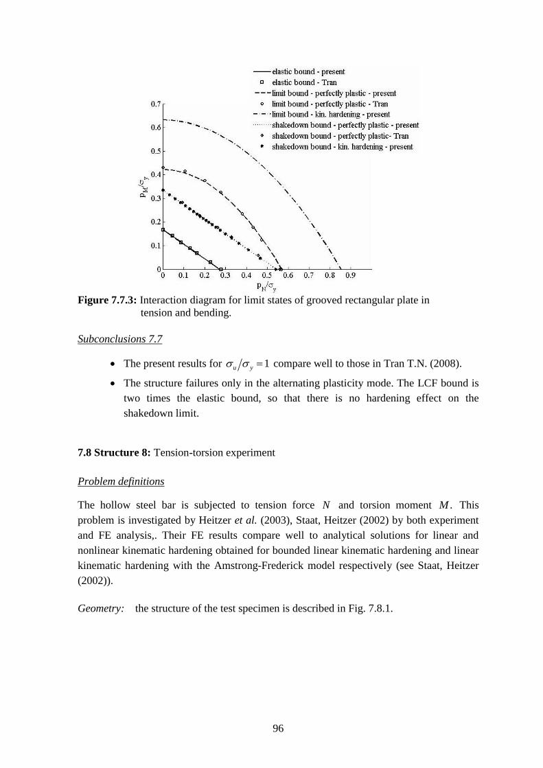
96

Figure 7.7.3: Interaction diagram for limit states of grooved rectangular plate in

tension and bending.

Subconclusions 7.7

The present results for 1u y compare well to those in Tran T.N. (2008).

The structure failures only in the alternating plasticity mode. The LCF bound is

two times the elastic bound, so that there is no hardening effect on the

shakedown limit.

7.8 Structure 8: Tension-torsion experiment

Problem definitions

The hollow steel bar is subjected to tension force N and torsion moment .M This

problem is investigated by Heitzer et al. (2003), Staat, Heitzer (2002) by both experiment

and FE analysis,. Their FE results compare well to analytical solutions for linear and

nonlinear kinematic hardening obtained for bounded linear kinematic hardening and linear

kinematic hardening with the Amstrong-Frederick model respectively (see Staat, Heitzer

(2002)).

Geometry: the structure of the test specimen is described in Fig. 7.8.1.

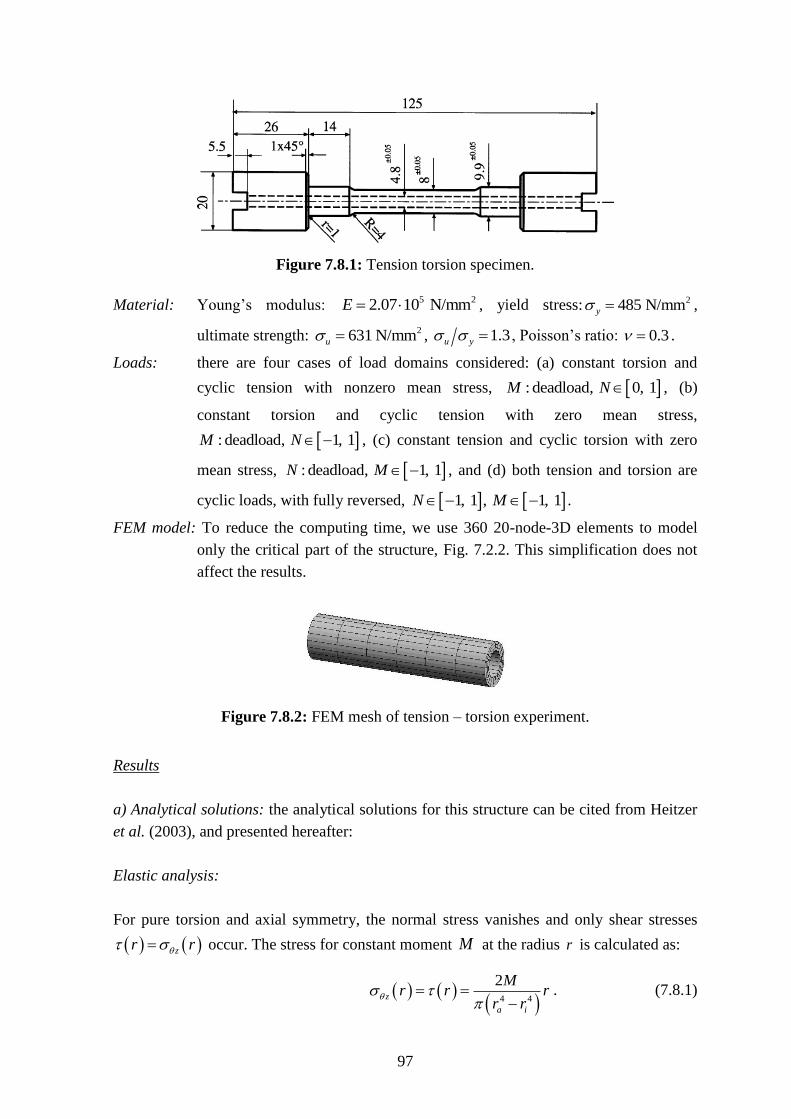
97

Figure 7.8.1: Tension torsion specimen.


ultimate strength: 2631 N/mmu , 1.3u y , Poisson’s ratio: 0.3 .

Loads: there are four cases of load domains considered: (a) constant torsion and

cyclic tension with nonzero mean stress, : deadload, 0, 1M N , (b)

constant torsion and cyclic tension with zero mean stress,

: deadload, 1, 1M N , (c) constant tension and cyclic torsion with zero

mean stress, : deadload, 1, 1N M , and (d) both tension and torsion are

cyclic loads, with fully reversed, 1, 1 , 1, 1N M .

FEM model: To reduce the computing time, we use 360 20-node-3D elements to model

only the critical part of the structure, Fig. 7.2.2. This simplification does not

affect the results.

Figure 7.8.2: FEM mesh of tension – torsion experiment.

Results

a) Analytical solutions: the analytical solutions for this structure can be cited from Heitzer

et al. (2003), and presented hereafter:

Elastic analysis:

For pure torsion and axial symmetry, the normal stress vanishes and only shear stresses

zr r occur. The stress for constant moment M at the radius r is calculated as:

4 4

2z

a i

Mr r r

r r

. (7.8.1)

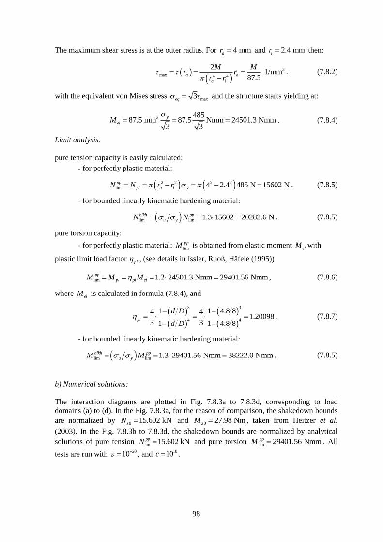
98

The maximum shear stress is at the outer radius. For 4 mmar and 2.4 mmir then:

3

max 4 4

2 1/mm

87.5a a

a i

M Mr r

r r

. (7.8.2)

with the equivalent von Mises stress max3eq and the structure starts yielding at:

3 48587.5 mm 87.5 Nmm 24501.3 Nmm

3 3

y

elM

. (7.8.4)

Limit analysis:

pure tension capacity is easily calculated:

- for perfectly plastic material:

2 2 2 2

lim 4 2.4 485 N 15602 Npp

pl a i yN N r r . (7.8.5)

- for bounded linearly kinematic hardening material:

lim lim 1.3 15602 20282.6 Nblkh pp

u yN N . (7.8.5)

pure torsion capacity:

- for perfectly plastic material: lim

ppM is obtained from elastic moment elM with

plastic limit load factor pl , (see details in Issler, Ruoß, Häfele (1995))

lim 1.2 24501.3 Nmm 29401.56 Nmmpp

pl pl elM M M , (7.8.6)

where elM is calculated in formula (7.8.4), and

3 3

4 4

1 1 4.8 84 41.20098

3 31 1 4.8 8pl

d D

d D

. (7.8.7)

- for bounded linearly kinematic hardening material:

lim lim 1.3 29401.56 Nmm 38222.0 Nmmblkh pp

u yM M . (7.8.5)

b) Numerical solutions:

The interaction diagrams are plotted in Fig. 7.8.3a to 7.8.3d, corresponding to load

domains (a) to (d). In the Fig. 7.8.3a, for the reason of comparison, the shakedown bounds

are normalized by 0 15.602 kNzN and 0 27.98 NmzM , taken from Heitzer et al.

(2003). In the Fig. 7.8.3b to 7.8.3d, the shakedown bounds are normalized by analytical

solutions of pure tension lim 15.602 kNppN and pure torsion lim 29401.56 NmmppM . All

tests are run with 2010 , and

1010c .

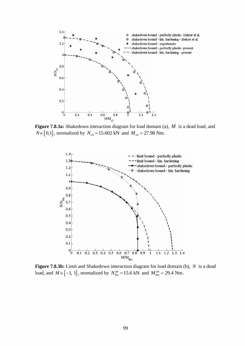
99

Figure 7.8.3a: Shakedown interaction diagram for load domain (a), M is a dead load, and

0,1N , normalized by 0 15.602 kNzN and 0 27.98 NmzM .

Figure 7.8.3b: Limit and Shakedown interaction diagram for load domain (b), N is a dead

load, and 1, 1M , normalized by lim 15.6 kNppN and lim 29.4 NmppM .

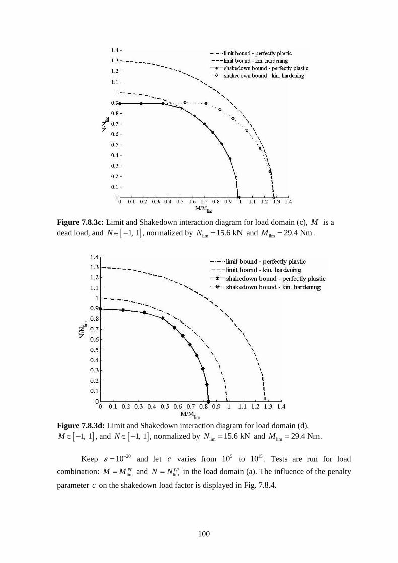
100

Figure 7.8.3c: Limit and Shakedown interaction diagram for load domain (c), M is a

dead load, and 1, 1N , normalized by lim 15.6 kNN and lim 29.4 NmM .

Figure 7.8.3d: Limit and Shakedown interaction diagram for load domain (d),

1, 1M , and 1, 1N , normalized by lim 15.6 kNN and lim 29.4 NmM .

Keep 2010 and let c varies from

510 to 1510 . Tests are run for load

combination: lim

ppM M and lim

ppN N in the load domain (a). The influence of the penalty

parameter c on the shakedown load factor is displayed in Fig. 7.8.4.

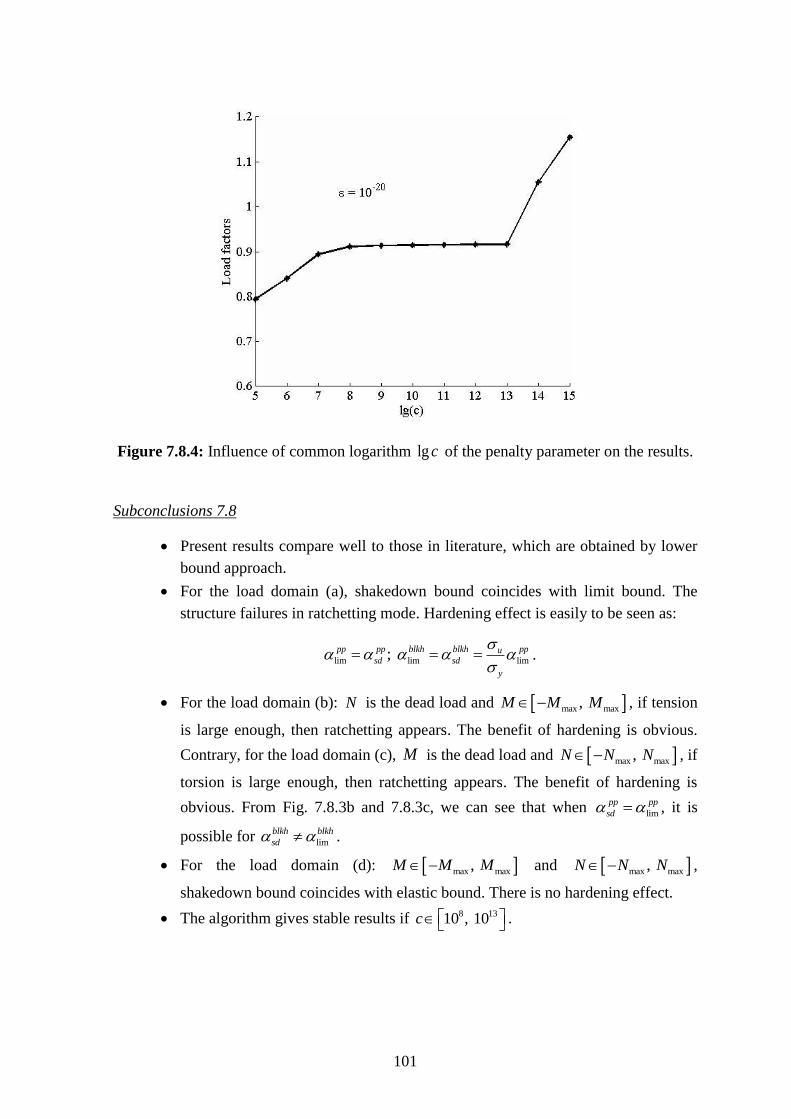
101

Figure 7.8.4: Influence of common logarithm lg c of the penalty parameter on the results.

Subconclusions 7.8

Present results compare well to those in literature, which are obtained by lower

bound approach.

For the load domain (a), shakedown bound coincides with limit bound. The

structure failures in ratchetting mode. Hardening effect is easily to be seen as:

lim lim lim; pp pp blkh blkh ppusd sd

y

.

For the load domain (b): N is the dead load and max max, M M M , if tension

is large enough, then ratchetting appears. The benefit of hardening is obvious.

Contrary, for the load domain (c), M is the dead load and max max, N N N , if

torsion is large enough, then ratchetting appears. The benefit of hardening is

obvious. From Fig. 7.8.3b and 7.8.3c, we can see that when lim

pp pp

sd , it is

possible for lim

blkh blkh

sd .

For the load domain (d): max max, M M M and max max, N N N ,

shakedown bound coincides with elastic bound. There is no hardening effect.

The algorithm gives stable results if 8 1310 , 10c .

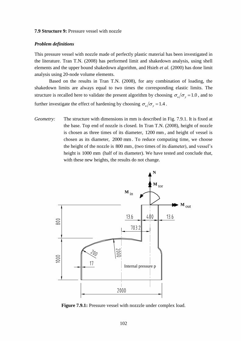
102

7.9 Structure 9: Pressure vessel with nozzle

Problem definitions

This pressure vessel with nozzle made of perfectly plastic material has been investigated in

the literature. Tran T.N. (2008) has performed limit and shakedown analysis, using shell

elements and the upper bound shakedown algorithm, and Hsieh et al. (2000) has done limit

analysis using 20-node volume elements.

Based on the results in Tran T.N. (2008), for any combination of loading, the

shakedown limits are always equal to two times the corresponding elastic limits. The

structure is recalled here to validate the present algorithm by choosing 1.0u y , and to

further investigate the effect of hardening by choosing 1.4u y .

Geometry: The structure with dimensions in mm is described in Fig. 7.9.1. It is fixed at

the base. Top end of nozzle is closed. In Tran T.N. (2008), height of nozzle

is chosen as three times of its diameter, 1200 mm , and height of vessel is

chosen as its diameter, 2000 mm . To reduce computing time, we choose

the height of the nozzle is 800 mm , (two times of its diameter), and vessel’s

height is 1000 mm (half of its diameter). We have tested and conclude that,

with these new heights, the results do not change.

Internal pressure p

M

M

M tor

N

in

out

Figure 7.9.1: Pressure vessel with nozzzle under complex load.

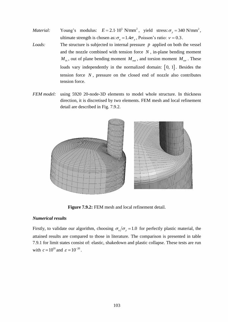
103


ultimate strength is chosen as: 1.4u y , Poisson’s ratio: 0.3 .

Loads: The structure is subjected to internal pressure p applied on both the vessel

and the nozzle combined with tension force N , in-plane bending moment

inM , out of plane bending moment outM , and torsion moment torM . These

loads vary independently in the normalized domain: 0, 1 . Besides the

tension force N , pressure on the closed end of nozzle also contributes

tension force.

FEM model: using 5920 20-node-3D elements to model whole structure. In thickness

direction, it is discretised by two elements. FEM mesh and local refinement

detail are described in Fig. 7.9.2.

Figure 7.9.2: FEM mesh and local refinement detail.

Numerical results

Firstly, to validate our algorithm, choosing 1.0u y for perfectly plastic material, the

attained results are compared to those in literature. The comparison is presented in table

7.9.1 for limit states consist of: elastic, shakedown and plastic collapse. These tests are run

with 1010c and

2010 .

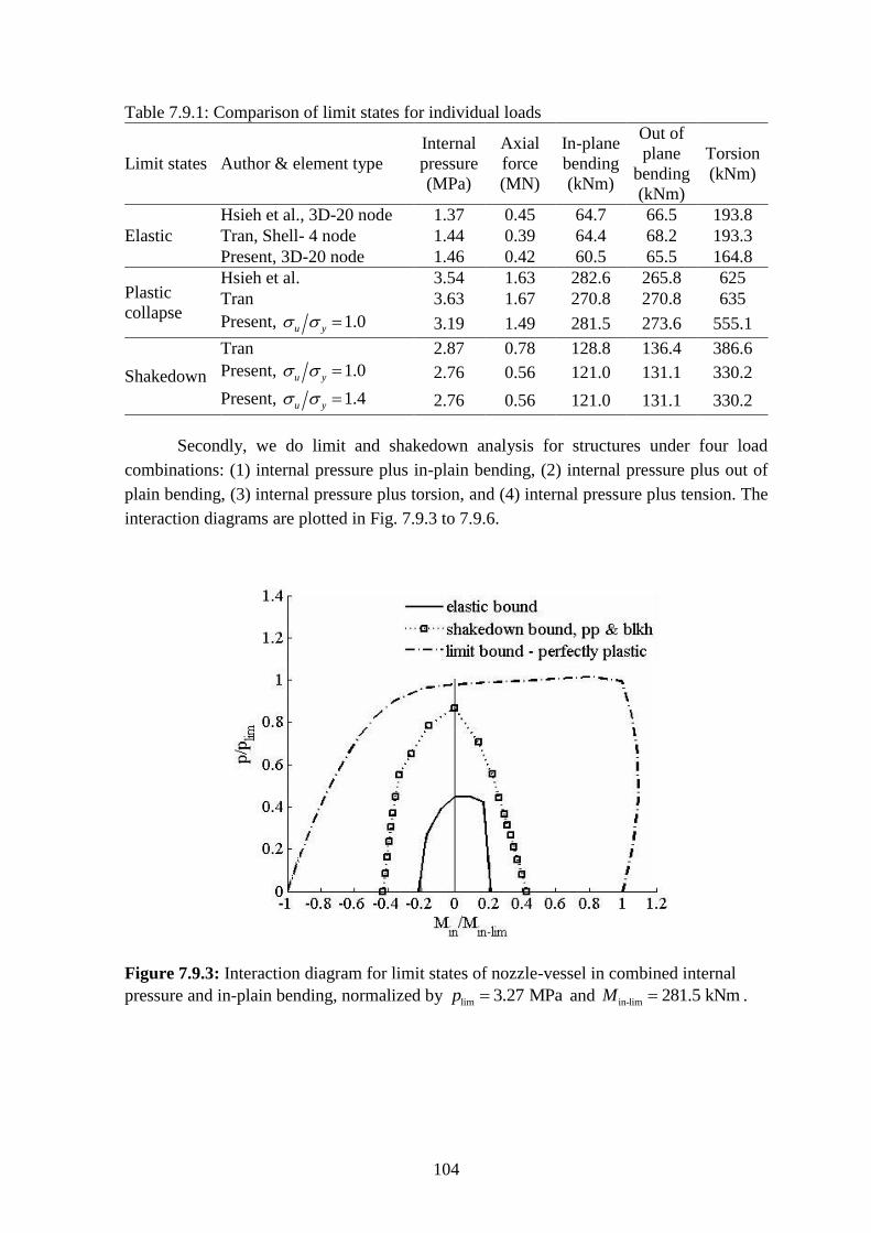
104

Table 7.9.1: Comparison of limit states for individual loads

Limit states Author & element type

Internal

pressure

(MPa)

Axial

force

(MN)

In-plane

bending

(kNm)

Out of

plane

bending

(kNm)

Torsion

(kNm)

Elastic

Hsieh et al., 3D-20 node 1.37 0.45 64.7 66.5 193.8

Tran, Shell- 4 node 1.44 0.39 64.4 68.2 193.3

Present, 3D-20 node 1.46 0.42 60.5 65.5 164.8

Plastic

collapse

Hsieh et al. 3.54 1.63 282.6 265.8 625

Tran 3.63 1.67 270.8 270.8 635

Present, 1.0u y 3.19 1.49 281.5 273.6 555.1

Shakedown

Tran 2.87 0.78 128.8 136.4 386.6

Present, 1.0u y 2.76 0.56 121.0 131.1 330.2

Present, 1.4u y 2.76 0.56 121.0 131.1 330.2

Secondly, we do limit and shakedown analysis for structures under four load

combinations: (1) internal pressure plus in-plain bending, (2) internal pressure plus out of

plain bending, (3) internal pressure plus torsion, and (4) internal pressure plus tension. The

interaction diagrams are plotted in Fig. 7.9.3 to 7.9.6.

Figure 7.9.3: Interaction diagram for limit states of nozzle-vessel in combined internal

pressure and in-plain bending, normalized by lim 3.27 MPap and in-lim 281.5 kNmM .

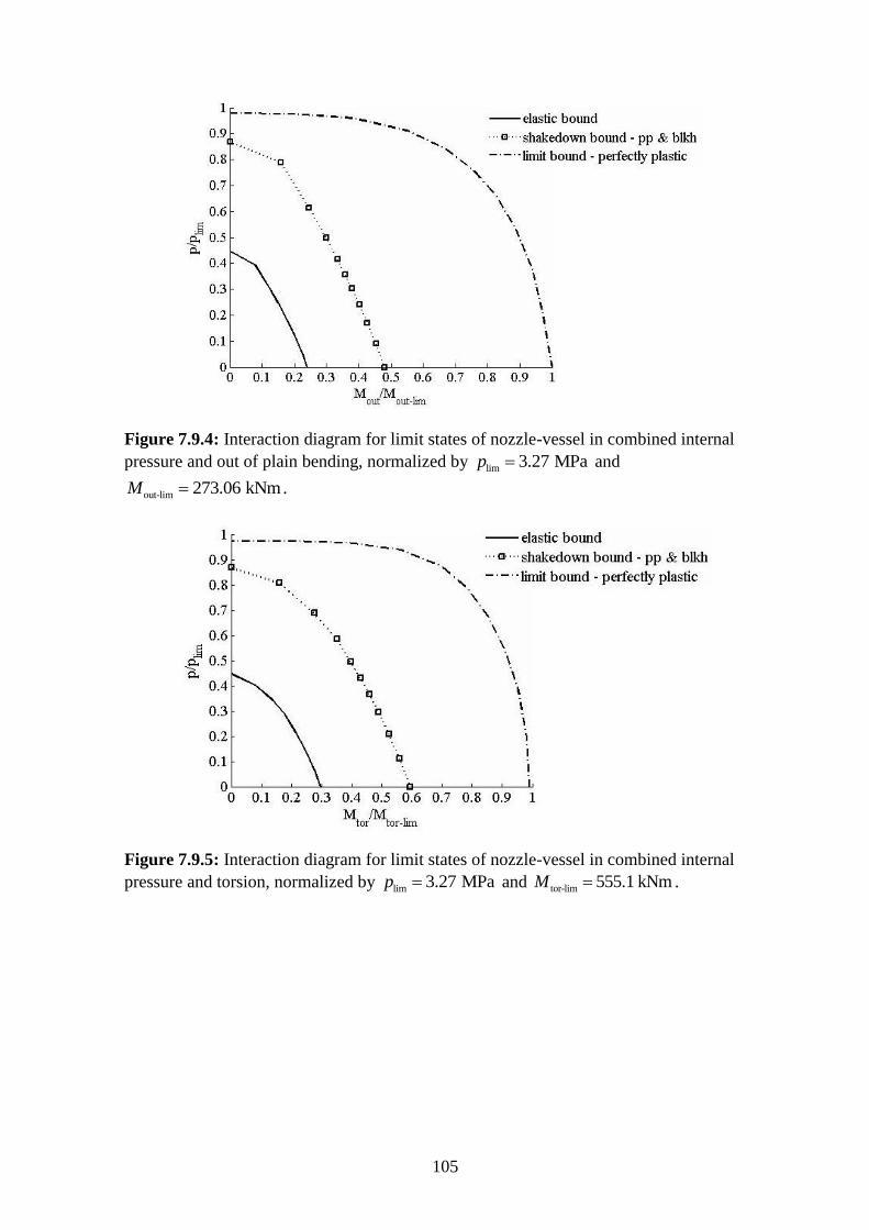
105


pressure and out of plain bending, normalized by lim 3.27 MPap and

out-lim 273.06 kNmM .


pressure and torsion, normalized by lim 3.27 MPap and tor-lim 555.1 kNmM .

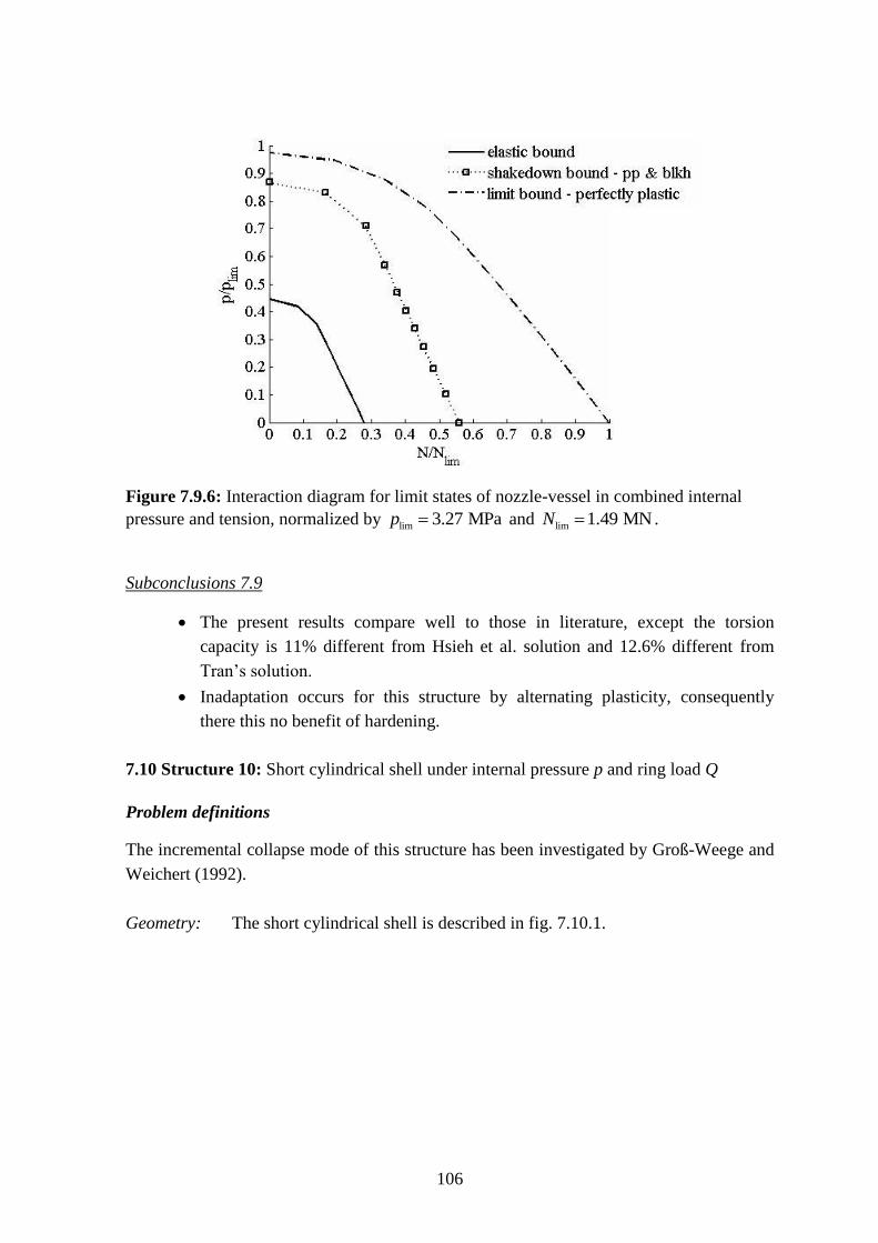
106


pressure and tension, normalized by lim 3.27 MPap and lim 1.49 MNN .

Subconclusions 7.9

The present results compare well to those in literature, except the torsion

capacity is 11% different from Hsieh et al. solution and 12.6% different from

Tran’s solution.

Inadaptation occurs for this structure by alternating plasticity, consequently

there this no benefit of hardening.

7.10 Structure 10: Short cylindrical shell under internal pressure p and ring load Q

Problem definitions

The incremental collapse mode of this structure has been investigated by Groß-Weege and

Weichert (1992).

Geometry: The short cylindrical shell is described in fig. 7.10.1.

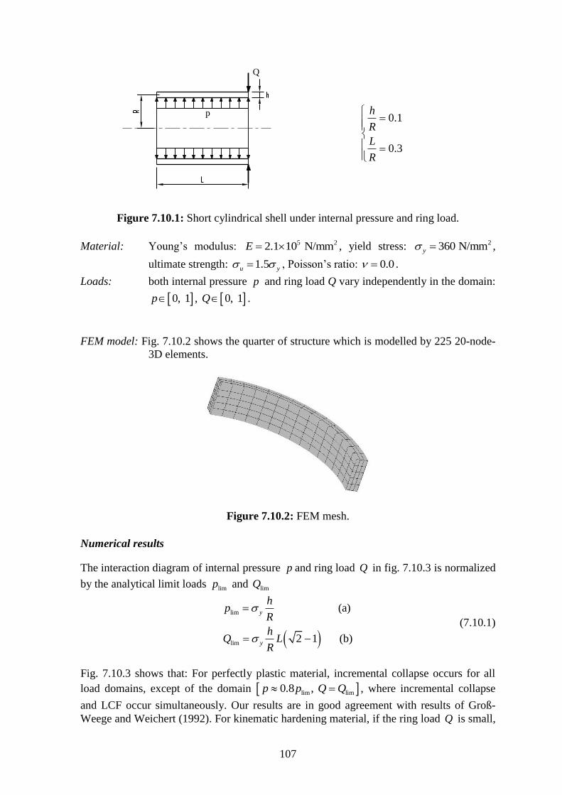
107

p

Q

0.1

0.3

h

R

L

R

Figure 7.10.1: Short cylindrical shell under internal pressure and ring load.



Loads: both internal pressure p and ring load Q vary independently in the domain:

0, 1p , 0, 1Q .

FEM model: Fig. 7.10.2 shows the quarter of structure which is modelled by 225 20-node-

3D elements.


Numerical results

The interaction diagram of internal pressure p and ring load Q in fig. 7.10.3 is normalized

by the analytical limit loads limp and limQ

lim

lim

(a)

2 1 (b)

y

y

hp

R

hQ L

R

(7.10.1)

Fig. 7.10.3 shows that: For perfectly plastic material, incremental collapse occurs for all

load domains, except of the domain lim lim0.8 , p p Q Q , where incremental collapse

and LCF occur simultaneously. Our results are in good agreement with results of Groß-

Weege and Weichert (1992). For kinematic hardening material, if the ring load Q is small,

108

only ratchetting occurs, hence the shakedown load multiplier of hardening material, blkh

sd ,

is u y times higher than the shakedown load multiplier of perfectly plastic material,

pp

sd . When Q is high enough, LCF occurs, hence blkh

sd is less than pp

u y sd , but of

course, greater than pp

sd .

Figure 7.10.3: Interaction diagram of internal pressure p and ring load Q for structure 10,

normalized by limp and limQ .

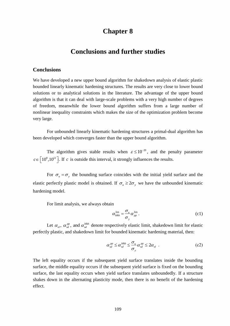
109

Chapter 8

Conclusions and further studies

Conclusions

We have developed a new upper bound algorithm for shakedown analysis of elastic plastic

bounded linearly kinematic hardening structures. The results are very close to lower bound

solutions or to analytical solutions in the literature. The advantage of the upper bound

algorithm is that it can deal with large-scale problems with a very high number of degrees

of freedom, meanwhile the lower bound algorithm suffers from a large number of

nonlinear inequality constraints which makes the size of the optimization problem become

very large.

For unbounded linearly kinematic hardening structures a primal-dual algorithm has

been developed which converges faster than the upper bound algorithm.

The algorithm gives stable results when 2010 , and the penalty parameter

8 1210 ,10c . If c is outside this interval, it strongly influences the results.

For u y the bounding surface coincides with the initial yield surface and the

elastic perfectly plastic model is obtained. If 2u y we have the unbounded kinematic

hardening model.

For limit analysis, we always obtain

lim limublkh pp

y

. (c1)

Let , , and pp blkh

el sd sd denote respectively elastic limit, shakedown limit for elastic

perfectly plastic, and shakedown limit for bounded kinematic hardening material, then:

2pp blkh ppusd sd sd el

y

. (c2)

The left equality occurs if the subsequent yield surface translates inside the bounding

surface, the middle equality occurs if the subsequent yield surface is fixed on the bounding

surface, the last equality occurs when yield surface translates unboundedly. If a structure

shakes down in the alternating plasticity mode, then there is no benefit of the hardening

effect.

110

For the sake of simplification, as stated in Pham D.C. (2007), we can use the

shakedown algorithm of elastic perfectly plastic material to do a shakedown analysis of

bounded kinematic hardening structures with replacing y by u to obtain the ratchetting

limit. However, this simplification ignores the inequalities in relation (c2).

The shakedown limit does not depend on the hardening curve, but only on the

initial yield stress y and the ultimate strength u .

Elastic analysis is sensitive to stress concentration such as sharp reentrant corners

of the geometry. As a consequence shakedown analysis shows the same sensitivity if the

failure is by alternating plasticity.

Further studies

Shakedown analysis for hardening structures can be developed for structural reliability

analysis, where geometry, material properties and applied loads are considered as random

variables.

The influence of temperature on material properties should be investigated, since

the hardening effect plays an important role for structures under thermal load. This is an

unsolved problem for temperature dependent elastic data (Oueslati, de Saxcé, 2009).

For more realistic modelling of hardening material, nonlinear kinematic hardening

should be considered although Staat, Heitzer (2002) showed that the bounded linearly

kinematic hardening model may give results which are quite close to the nonlinear

Frederick-Armstrong model.

Mixed models which combine isotropic and kinematic hardening model should be

investigated. The subsequent yield surface may also change its shape. In most cases no

detailed information is available for such complicated material. It is one of the great

advantages of shakedown analysis that it can give robust results with incomplete

information on material models and load history. Therefore is may be recommended to

first study if complex material models give shakedown limits which differ from the limits

obtained with more simple models. This would help make a decision about the necessary

effort in theory and material testing.

111

References:

[1] Abdel-Karim M., Ohno N. Kinematic hardening model suitable for ratchetting

with steady-state. International Journal of Plasticity 16 (2000) 225-240.

[2] Andersen K.D., Christiansen E. Limit analysis with the dual affine scaling

algorithm. Journal of Computational and Applied Mathematics 59 (1995) 233-

243.

[3] Anderson I.A., Collins I.F. Plane strain stress distributions in discrete and blended

coasted solids under normal and sliding contact. Wear 185 (1995) 23-33.

[4] Artioli E., Auricchio F., Beirão da Veiga L. Second-order accurate integration

algorithms for von-Mises plasticity with a nonlinear kinematic hardening

mechanism. Comput. Methods Appl. Mech. Engrg. 196 (2007) 1827–1846.

[5] Bari Shafiqul, Hassan Tasnim. An advancement in cyclic plasticity modelling for

multiaxial ratchetting simulation. International Journal of Plasticity 18 (2002)

873–894.

[6] Bari Shafiqul, Hassan Tasnim. Kinematic hardening rules in uncoupled modelling

for multiaxial ratchetting simulation. International Journal of Plasticity 17 (2001)

885–905.

[7] Bazaraa M.S., Sherali H.D., Shetty C.M. Nonlinear programming Theory and

Algorithms. John Wiley & Sons, Inc., New York (2006).

[8] Belytschko T. Plane stress shakedown analysis by finite elements. Int. J. Mech.

Sci. 14, (1972) 619-625.

[9] Bisbos C.D., Pardalos P.M. Second-order cone and semidefinite representations of

material failure criteria. Journal of Optimization Theory and Applications, 134 (2),

(2007) 275-301. http://dx.doi.org/10.1007/s10957-007-9243-8

[10] Bisbos C.D., Papaioannou G. Shakedown analysis of FEM-discretized steel shell

structures under the Ilyushin yield criterion. In Baniotopoulos C.C. (ed.): II. Int.

Conference on Nonsmooth Nonconvex Mechanics with Applications in

Engineering (II. NNMAE), Thessaloniki, July 7-8, (2006) 197-204.

[11] Bodovillé G., de Saxcé G. Plasticity with non-linear kinematic hardening-

modelling and shakedown analysis by the bipotential approach. Eur. J. Mech.

A/Solids 20 (2001) 99–112.

[12] Boulbibane M., Weichert D. Application of shakedown theory to soils with non-

associated flow rules. Mechanics Research Communications, 24 (5), (1997) 513-

519.

[13] Bousshine L., Chaaba A., de Saxcé G. Plastic limit load of plane frames with

frictional contact supports. International Journal of Mechanical Sciences 44

(2002) 2189–2216.

[14] Bouby C., de Saxcé G., Tritsch J.-B. A comparison between analytical

calculations of the shakedown load by the bipotential approach and step-by-step

computations for elastoplastic materials with nonlinear kinematic hardening.

International Journal of Solids and Structures 43 (2006) 2670–2692.

http://dx.doi.org/10.1007/s10957-007-9243-8

112

[15] Bower A.F. Mechanic of solids. CRC Press, Boca Raton (2010).

[16] Capsoni A., Corradi L. A plane strain formulation of the elastic-plastic

constitutive law for hardening von Mises materials. Int. J. Solids Structures 32

(23), (1995) 3515-3531.

[17] Carvelli V. Shakedown analysis of unidirectional fiber reinforced metal matrix

composites. Computational Materials Science 31 (2004) 24-32.

[18] Casciaro R., Cascini L. A mixed formulation and mixed elements for limit

analysis. Int. J. Num. Meth. In Eng., 18 (1982) 211-243.

[19] Chaboche J.L. A review of some plasticity and viscoplasticity constitutive

theories. International Journal of Plasticity 24 (2008) 1642–1693.

[20] Chen Haofeng, Ponter A.R.S. A method for the evaluation of a ratchet limit and

the amplitude. Eur. J. Mech. A/Solids 20 (2001) 555–571.

[21] Chen Xu, Jiao R., Kim K.S. Simulation of ratchetting strain to a high number of

cycles under biaxial loading. International Journal of Solids and Structures 40

(2003) 7449–7461.

[22] Chen Xu, Jiao R. Modified kinematic hardening rule for multiaxial ratchetting

prediction. International Journal of Plasticity 20 (2004) 871–898.

[23] Christensen Peter W. A nonsmooth Newton method for elastoplastic problems.

Comput. Methods Appl. Mech. Engrg. 191 (2002) 1189-2019.

[24] Cocchetti G., Maier G. Elastic–plastic and limit-state analyses of frames with

softening plastic-hinge models by mathematical programming. International

Journal of Solids and Structures 40 (2003) 7219–7244.

[25] Code_Aster 7.3. User’s manual. A product of EDF R&D, Clamart, France (2003).

http://www.code-aster.org

[26] Colak Ozgen U. Kinematic hardening rules for modelling uniaxial and multiaxial

ratchetting. Materials and Design 29 (2008) 1575–1581.

[27] Corona E., Hassan T. and Kyriakides S. On the performance of kinematic

hardening rules in predicting a class of biaxial ratchetting histories. International

Journal of Plasticity, 12 (1), (1996) 117-145.

[28] Chang T.Y., Chu S.C. Elastic-plastic deformation of cylindrical pressure vessels

under cyclic loading. Nuclear Engineering and Design 27 (1974) 228-237.

[29] De Saxcé G., Tritsch J.B., Hjiaj M. Shakedown of elastic-plastic structure with

nonlinear kinematic hardening by the bipotential approach, in D. Weichert, G.

Maier eds., Inelastic Analysis of Structures under Variable Loads, Kluwer,

Dordrecht, (2000), 167-182.

[30] Druyanov B., Roman I. Concept of the limit yield condition in shakedown theory.

Int. J. Solids Structures 34 (13) (1997) 1547-1556.

[31] El Abdi R., Samrout H. A non-linear kinematic hardening model for a steel under

complex loadings. Computers and Structures 76 (2000) 675-681.

http://www.code-aster.org/

113

[32] Fedele R., Filippini M., Maier G. Constitutive model calibration for railway wheel

steel through tension–torsion tests. Computers and Structures 83 (2005) 1005–

1020.

[33] Feng Xi-Qiao, Liu Xin-Sheng. On shakedown of three-dimensional elastoplastic

strain-hardening structures. International Journal of Plasticity, 12 (10) (1997)

1241-1256.

[34] Fortin J., Hjiaj M., de Saxcé G. An improved discrete element method based on a

variational formulation of the frictional contact law. Computers and Geotechnics

29 (2002) 609–640.

[35] Fung Y.C., Pin Tong. Classical and computational solid mechanics, Advanced

Series in Engineering Science- Vol. 1, World Scientific Publishing, Singapore

2001.

[36] Gao Bingjun, Chen Xu, Chen Gang. Ratchetting and ratchetting boundary study of

pressurized straight low carbon steel pipe under reversed bending. International

Journal of Pressure Vessels and Piping 83 (2006) 96–106.

[37] Garcea G., Armentano G., Petrolo S., Casciaro R. Finite element shakedown of

two-dimensional structures. Int. J. Numer. Mech. Engng 63 (2005) 1174-1202.

[38] Gaydon F.A. On the yield-point loading of a square plate with concentric circular

hole. Journal of the Mechanics and Physics of Solids, 2, (1954) 170 – 175.

[39] Gaydon F.A., McCrum A.W. A theoretical investigation of the yield point loading

of a square plate with central circular hole. Journal of the Mechanics and Physics

of Solids, 2, (1954) 156 -169.

[40] GiD 7.2. User’s manual. A product of Centre for Numerical Methods in

Engineering (CIMNE), Barcelona (2002). http://www.gid.cimne.upc.es

[41] Gokhfeld D.A., Cherniavsky O.F. Limit analysis of structures at thermal cycling,

Sijthoff & Noordhoff, The Netherlands (1980).

[42] Groß-Weege J. On the numerical investigation of the shakedown behaviour of

shells (in German). ZAMM 69, (1989) 480

[43] Groß-Weege J. A unified formulation of statical shakedown criteria for

geometrically nonlinear problems. Int. J. Plasticity 6 (1990) 433.

[44] Groß-Weege J., Weichert D. Elastic-Plastic shells under variable mechanical and

thermal loads. Int. J. Mech. Sci, 34 (11), (1992) 863-880.

[45] Hachemi A., Weichert D. Application of shakedown theory to damaging inelastic

material under mechanical and thermal load. Int. J. Mech. Sci, Vol. 39, No. 9,

(1997) 1067-1076.

[46] Hahm J.H., Kim K.H. Anisotropic work hardening of steel sheets under plane

stress. International Journal of Plasticity 24 (2008) 1097-1127.

[47] Halphen B., Nguyen Q.S. Sur les matériaux standards généralisés. J. Méc. 14,

(1975) 39-63.

http://www.gid.cimne.upc.es/

114

[48] Hamadouche M.A., Weichert D. Application of shakedown theory to soil

dynamics. Mechanics Research Communications, 26 (5), (1999) 565-574.

[49] Hassan Tasnim, Zhu Yimin, Matzen V.C. Improved ratchetting analysis of piping

components. International Journal of Pressure Vessels and Piping 75 (1998) 643–

652.

[50] Hassan Tasnim, Taleb Lakhdar, Krishna Shree. Influence of non-proportional

loading on ratchetting responses and simulations by two recent cyclic plasticity

models. International Journal of Plasticity 24 (2008) 1863–1889.

[51] Heitzer M. Traglast- und Einspielanalyse zur Bewertung der Sicherheit passiver

Komponenten. Jül-3704 Report of Forschungszentrum Jülich, Ph.D. Thesis

RWTH Aachen (1999).

[52] Heitzer M., Pop G., Staat M. Basic reduction for the shakedown problem for

bounded kinematic hardening material. J. Global optimization, 17 (2000), 185-

200.

[53] Heitzer M., Staat M. FEM-computation of load carrying capacity of highly loaded

passive components by direct methods. Nuclear Engineering and Design, 193 (3),

(1999) 349-358. http://dx.doi.org/10.1016/S0029-5493(99)00190-9

[54] Heitzer M., Staat M. Basis reduction technique for limit and shakedown problems.

In [Staat, Heitzer (2003), 1-55].

[55] Heitzer M., Staat M., Reiners H., Schubert F. Shakedown and ratchetting under

tension–torsion loadings_analysis and experiments. Nuclear Engineering and

Design 225 (2003) 11–26.

[56] Hsieh M.F., Moffat D.G., Mistry J. Nozzles in the knuckle region of a

torispherical head: limit load interaction under combined pressure and piping

loads. Int. J. Pres. Vessels and Piping, 77, (2000) 807-815.

[57] Huang Y., Stein E. Shakedown of a cracked body consisting kinematic hardening

material. Engineering Fracture Mechanics 54 (1), (1996) 107-112.

[58] Issler L., Ruoß H., Häfele P. Festigkeitslehre Grundlagen, Springer, Berlin

Heidelberg (1995).

[59] Jospin J.R. Displacement estimates of pipe elbows prior to plastic collapse loads.

Nuclear Engineering and Design 178 (1997) 165–178.

[60] Kang Guozheng, Ohno Nobutada, Nebu Akira. Constitutive modelling of strain

range dependent cyclic hardening. International Journal of Plasticity 19 (2003)

1801–1819.

[61] Kapoor A., Johnson K.L. Plastic ratchetting as a mechanism of metallic wear.

Proceedings of the Royal Society of London Series A 445 (1994) 367–381.

[62] Kobayashi M. and Ohno N. Thermal ratchetting of a cylinder subjected to a

moving temperature front Effects of kinematic hardening rules on the analysis.

International Journal of Plasticity, 12 (2), (1996) 255-271.

http://dx.doi.org/10.1016/S0029-5493(99)00190-9

115

[63] Kan Q.H., Kang G.Z., Zhang J. Uniaxial time-dependent ratchetting visco-plastic

model and finite element application. Theoretical and Applied Fracture

Mechanics 47 (2007) 133–144.

[64] König J.A. Shakedown of Elastic-Plastic Structures, PWN-Polish Scientific

Publishers, Warsaw, and Elsevier, Amsterdam (1987)

[65] König J.A., Kleiber M. On a new method of shakedown analysis. Bulletin

del’Academie Polonaise des Sciences, Serie des sciences techniques 26 (1978)

165-171.

[66] Kunc R., Prebil I. Low-cycle fatigue properties of steel 42CrMo4. Materials

Science and Engineering A345 (2003) 278-285.

[67] Krieg R.D., Xu Shiqiang. Plane stress linear hardening plasticity theory. Finite

Elements in Analysis and Design 27 (1997) 41-67.

[68] Kulkarni S.C., Desai Y.M., Kant T., Reddy G.R., Prasad P., Vaze K.K., Gupta C.

Uniaxial and biaxial ratchetting in piping materials–experiments and analysis.

International Journal of Pressure Vessels and Piping 81 (2004) 609-617.

[69] Khoei A.R., Jamali N. On the implementation of a multi-surface kinematic

hardening plasticity and its applications. International Journal of Plasticity 21

(2005) 1741-1770.

[70] Krämer D., Krolop S., Scheffold A., Stegmeyer R. Investigations into the

ratchetting behaviour of austenitic pipes. Nuclear Engineering and Design 171

(1997) 161-172.

[71] Lakhdar Taleb, Cailletaud G., Liliana Blaj. Numerical simulation of complex

ratchetting tests with a multi-mechanism model type. International Journal of

Plasticity 22 (2006) 724–753.

[72] Lemaitre J., Chaboche J.L. Mechanics of solid materials. University press,

Cambridge (2000).

[73] Li H.X., Yu H.S. A nonlinear programming approach to kinematic shakedown

analysis of frictional materials. International Journal of Solids and Structures 43

(2006) 6594-6614.

[74] Liu G.R., Nguyen T.T. Smoothed Finite Element Methods. CRC Press, Boca

Raton (2010)

[75] Lubliner J. Plasticity Theory. Revised edition, University of California at Berkeley

(2005).

[76] Melan E. Theorie statisch unbestimmter Systeme aus ideal plastischem Baustoff.

Sitzber. Akad. Wiss. Wien IIa, 145 (1936) 195-218.

[77] Melan E. Zur Plastizität des räumlichen Kontinuums. Ing.-Arch. 8 (1938) 116-

126.

[78] Makrodimopoulos A., Bisbos C. Shakedown analysis of plane stress problems via

SOCP. (In Staat M., Heitzer M. (eds.) Numerical Methods for Limit and

Shakedown analysis – Deterministic and Probabilistic Problems. NIC Series Vol.

116

15, John von Neumann Institute for Computing, Jülich (2003). http://www.fz-

juelich.de/nic-series/volume15/nic-series-band15.pdf ).

[79] Mahbadi H., Eslami M.R. Cyclic loading of beams based on the Prager and

Frederick–Armstrong kinematic hardening models. International Journal of

Mechanical Sciences 44 (2002) 859–879.

[80] Mahbadi H., Eslami M.R. Cyclic loading of thick vessels based on the Prager and

Armstrong–Frederick kinematic hardening models. International Journal of

Pressure Vessels and Piping 83 (2006) 409–419.

[81] Maier G. Shakedown theory in perfect elastoplasticity with associated and

nonassociated flow-laws: A finite element, linear programming approach.

Meccanica 4, (1969) 250-260.

[82] Maier G.A shakedown matrix theory allowing for work hardening and second-

order geometric effects. In: Foundations of plasticity (Sawczuk A., ed.), North-

Holland, Amsterdam (1973) 417-433.

[83] Mohammad Abdel-Karim. Numerical integration method for kinematic hardening

rules with partial activation of dynamic recovery term. International Journal of

Plasticity 21 (2005) 1303–1321.

[84] Mohammad Abdel-Karim. Shakedown of complex structures according to various

hardening rules. International Journal of Pressure Vessels and Piping 82 (2005)

427–458.

[85] Nadarajah C., Mackenzie D., Boyle J.T. Limit and shakedown analysis of nozzle

cylinder intersections under internal pressure and in-plane moment loading. Int. J.

Pres. Ves. & Piping 68 (1996) 261-272.

[86] Navarro A., Giráldez J.M., Vallellano C. A constitutive model for elastoplastic

deformation under variable amplitude multiaxial cyclic loading. International

Journal of Fatigue 27 (2005) 838–846.

[87] Nayebi A., El Abd R. Shakedown analysis of beams using nonlinear kinematic

hardening materials coupled with continuum damage mechanics. International

Journal of Mechanical Sciences 50 (2008) 1247-1254.

[88] Nguyen Q.S. On shakedown analysis in hardening. Journal of the Mechanics and

Physics of Solids 51 (2003) 101-125.

[89] Nguyen Q.S., Pham D.C. On shakedown theorems in hardening plasticity. C. R.

Acad. Sci. Paris, t. 329, Série II b, (2001) 307–314.

[90] Ohno N. and Wang J. Nonisothermal constitutive modelling of inelasticity based

on bounding surface. Nuclear Engineering and Design 133 (1992) 369-381.

[91] Ohno N., Wang J. On modelling of kinematic hardening for ratchetting behaviour.

Nuclear Engineering and Design 153 (1995) 205-212.

[92] Ohno N. Constitutive modelling of cyclic plasticity with emphasis on ratchetting.

Int. J. Mech. Sci. 40 (2-3), (1998) 251-261.

http://www.fz-juelich.de/nic-series/volume15/nic-series-band15.pdf


117

[93] Oueslati A., de Saxcé G. Static shakedown theorem for solids with btemperature

dependent elastic modulus. In: A.R.S. Ponter, D. Weichert, (eds.) Limit States of

Materials and Structures: Direct Methods. Springer, Netherlands (2009).

[94] Pham D.C. Shakedown theory for elastic-perfectly plastic bodies revisited.

International Journal of Mechanical Sciences 45 (2003) 1011-1027.

[95] Pham D.C. Shakedown static and kinematic theorems for elastic-plastic limited

linear kinematic-hardening solids. European Journal of Mechanics A/Solids 24

(2005) 35–45.

[96] Pham D.C. Shakedown theory for elastic plastic kinematic hardening bodies.

International Journal of Plasticity 23 (2007) 1240–1259.

[97] Pham D.C., Weichert D. Shakedown analysis for elastic plastic bodies with

limited kinematic hardening. Proc. Roy. Soc. London A 457 (2001) 1097-1110.

[98] Phạm P.T., Staat M. An upper bound algorithm for limit and shakedown analysis

of bounded linear kinematic hardening bodies. In: G. de Saxcé, et al. (eds.) Direct

Methods. Springer Netherlands, accepted.

[99] Phạm P.T., Vũ Đ.K., Trần T.N., Staat M. A primal-dual algorithm for shakedown

analysis of elastic-plastic bounded linearly kinematic hardening bodies. IV

European Conference on Computational Mechanics (ECCM 2010), Paris, France,

May 16-21, 2010.

[100] Polizzotto C. Upper bounds on plastic strains for elstic-perfectly plastic solids

subjected to variable loads. Int. J. Mech. Sci., 21 (1979) 317-327.

[101] Polizzotto C. Dynamic shakedown of elastic-plastic solids for a set of alternative

loading histories. Int. J. Non-Linear Mechanics. 19 (4) (1984) 363-371.

[102] Polizzotto C. A bounding technique for dynamic plastic deformations of damped

structures. Nuclear Engineering and Design 79 (1984) 363-376.

[103] Polizzotto C., Borino G., Caddemi S., Fuschi P. Shakedown problem for material

with internal variables. Eur. J. Mech. A./Solids, 10 (6) (1991) 621-639.

[104] Polizzotto C., Borino G. Shakedown and steady-state responses of elastic-plastic

solids in large displacements. Int. J. Solids Structures 33 (23) (1996) 3415-3437.

[105] Polizzotto C. Shakedown of elastic - plastic solids with frictionless unilateral

contact boundary conditions. Int. J. Mech. Sci. 39 (7) (1997) 819-828.

[106] Polizzotto C. Variational methods for the steady state response of elastic–plastic

solids subjected to cyclic loads. International Journal of Solids and Structures 40

(2003) 2673–2697.

[107] Polizzotto C. Shakedown theorems for elastic–plastic solids in the framework of

gradient plasticity. International Journal of Plasticity 24 (2008) 218–241.

[108] Ponter A.R.S., Chen Haofeng. A minimum theorem for cyclic load in excess of

shakedown, with application to the evaluation of a ratchet limit. Eur. J. Mech.

A/Solids 20 (2001) 539–553.

118

[109] Ponter A.R.S., Chen H.F., Ciavarella M., Specchia G. Shakedown analysis for

rolling and sliding contact problems. International Journal of Solids and

Structures 43 (2006) 4201–4219.

[110] Ponter A.R.S., Engelhardt M. Shakedown limits for a general yield condition-

implementation and application for a Von Mises yield condition. Eur. J. Mech.

A/Solids 19 (2000) 423–445.

[111] Ponter A.R.S., Fuschi P., Engelhardt M. Limit analysis for a general class of yield

conditions. Eur. J. Mech. A/Solids 19 (2000) 401–421.

[112] Ponter A. R. S., Leckie F. A. Bounding properties of metal-matrix composites

subjected to cyclic thermal loading. J. Mech. Phys. Solids, 46 (4), (1998a) 697-

717.

[113] Ponter A. R. S., Leckie F. A. On the behaviour of metal matrix composites

subjected to cyclic thermal loading. J. Mech. Phys. Solids, 46 (11), (1998b) 2183-

2199.

[114] Portier L., Calloch S., Marquis D., Geyer P. Ratchetting under tension–torsion

loadings experiments and modelling. International Journal of Plasticity 16 (2000)

303-335.

[115] Prager W. A new method of analysing Stress and Strain in Work Hardening

Plastic Solids. J. Applied Mechanics, 23 (1956), 493-496.

[116] Prager W., Hodge P.G. Jr. Theory of perfectly plastic solids. Wiley, New York

(1951).

[117] Prager W. (1956) A new method of analyzing stress and strain in work hardening

plastic solids. J. Appl. Mech. ASME, 23 (1956) 493-496.

[118] Puzrin A.M., Houlsby G.T. Fundamentals of kinematic hardening hyperplasticity.

International Journal of Solids and Structures 38 (2001) 3771-3794.

[119] Queiroz F.J.R., Oden J.T., Ponter A.R.S., Barrosd Felicio B. A posteriori error

estimator and adaptive procedures for computation of shakedown and limit loads

on pressure vessels. Comput. Methods Appl. Mech. Engrg. 150 (1997) 155-171.

[120] Queiroz F.J.R., Ponter A.R.S., Barros Felício Bruzzi. Adaptive F.E. method for

the shakedown and limit analysis of pressure vessels. European Journal of

Mechanics A/Solids 22 (2003) 525–533.

[121] Rahman Syed M., Hassan Tasnim, Corona E. Evaluation of cyclic plasticity

models in ratchetting simulation of straight pipes under cyclic bending and steady

internal pressure. International Journal of Plasticity 24 (2008) 1756–1791.

[122] Savaidis A., Savaidis G., Zhang Ch. Elastic-plastic FE analysis of a notched shaft

under multiaxial nonproportional synchronous cyclic loading. Theoretical and

Applied Fracture Mechanics 36 (2001) 87-97.

[123] Savaidis A., Savaidis G., Zhang Ch. FE fatigue analysis of notched elastic–plastic

shaft under multiaxial loading consisting of constant and cyclic components.

International Journal of Fatigue 23 (2001) 303–315.

119

[124] Savaidis A., Savaidis G., Zhang Ch. Elastic-plastic FE analysis of a notched

cylinder under multiaxial nonproportional fatigue loading with variable

amplitudes. Computers and Structures 80 (2002) 1907–1918.

[125] Sarbayev B.S. On the theory of plasticity of anisotropic solids with isotropic and

kinematic hardening. Computational Materials Science 6 (1996) 21 l-224.

[126] Sawczuk A. On incremental collapse of shells and under cyclic loading. In:

Theory of the thin shells (Niordson F.I., ed.), Springer, Berlin (1969a) 328-340.

[127] Sawczuk A. Evaluation of upper bounds to shakedown loads for shells. J. Mech.

Phys. Solids 17(1969b) 291-231.

[128] Sawczuk A. Shakedown analysis of elastic-plastic structures. Nuclear engineering

and design 28 (1974) 121-136.

[129] Sai K., Cailletaud G. Multi-mechanism models for the description of ratchetting

Effect of the scale transition rule and of the coupling between hardening variables.

International Journal of Plasticity 23 (2007) 1589–1617.

[130] Schiffner K. Overlay models for structural analysis under cyclic loading.

Computers & Strucrures 56 (2/3) (1995) 321-328.

[131] Schwabe F. Einspieluntersuchungen von Verbundwerkstoffen mit periodischer

Mikrostruktur. Ph.D. Thesis, RWTH Aachen (2000).

[132] Shahram Sarkani, Michaelov G., Kihl D.P. Stochastic fatigue damage

accumulation in a T-welded joint accounting for the residual stress fields.

International Journal of Fatigue 23 (2001) S71–S78.

[133] Skodeli M.-A.A, Bisbos C.D. Limit and shakedown analysis of 3D frames via

approximate ellipoidal yiels surfaces. Engineering Structures 32 (2010) 1556-

1557.

[134] Staat M., Heitzer M. Limit and shakedown analysis for plastic safety of complex

structures. Transactions of the 14th

International Conference on Structural

Mechanics in Reactor Technology (SMiRT 14), Lyon, France, August 17-22

(1997). http://www.iasmirt.org/SMiRT14/B02-2

[135] Staat M., Heitzer M. Limit and shakedown analysis for design. Proceeding of 7th

German-Japanese Joint Seminar on Research in Structural Strength and NDE-

Problems in Nuclear Engineering, Stuttgart (1997) 4.3.1-4.3.19.

[136] Staat M., Heitzer M. LISA – a European project for FEM-based limit and

shakedown analysis. Nuclear Engineering and Design, 206 (2-3), (2001) 151-166.

http://dx.doi.org/10.1016/S0029-5493(00)00415-5

[137] Staat M. Some achievements of the European project LISA for FEM based limit

and shakedown analysis. In N. Badie (ed.) Computational Mechanics:

Developments and Applications - 2002. ASME PVP Vol. 441, Paper PVP2002-

1300, (2002) 177-185.

[138] Staat M., Heitzer M. The restricted influence of kinematic hardening on

shakedown loads. Proceedings of WCCM V, 5th World Congress on

http://www.iasmirt.org/SMiRT14/B02-2

http://dx.doi.org/10.1016/S0029-5493(00)00415-5

120

Computational Mechanics, Vienna, Austria, July 7-12 (2002).

http://opus.bibliothek.fh-aachen.de/opus/volltexte/2005/79/

[139] Staat M., Heitzer M. (eds.) Numerical Methods for Limit and Shakedown analysis

– Deterministic and Probabilistic Problems. NIC Series Vol. 15, John von

Neumann Institute for Computing, Jülich (2003). http://www.fz-juelich.de/nic-

series/volume15/nic-series-band15.pdf

[140] Staat M., Heitzer M., Lang H., Wirtz K. Direct finite element route for design-by-

analysis of pressure components. Int. J. Pressure Vessels Piping, 82 (1), (2005)

61-67. http://dx.doi.org/10.1016/j.ijpvp.2004.04.006

[141] Stein E., Huang Y.J. Shakedown for systems of kinematic hardening materials. In:

Inelastic behaviour of structures under variables loads (Mroz et al., eds.). Kluwer

Academic Publishers, (1995) 33-50.

[142] Stein E., Zhang G. Theoretical and numerical shakedown analysis for kinematic

hardening materials. Computational plasticity Fundamentals and applications. In:

prceeding of the international conference in Barcelona, Spain, 6-10th

April (Owen

D.R.J, Oñate E. and Hinton E., eds.), Pineridge Press, (1992) 1-26.

[143] Stein E., Zhang G., Huang Y. Modelling and computation of shakedown problems

for nonlinear hardening materials. Computer Methods in Applied Mechanics and

Engineering, 103 (1993) 247-272.

[144] Stein E., Zhang G., König J.A. Shakedown with nonlinear strain hardening

including structural computation using finite element method. Int. J. Plasticity, 8

(1992) 1-31.

[145] Stein E., Zhang G., Mahnken R. Shakedown analysis for perfectly plastic and

kinematic hardening materials. In: Progress in Computational Analysis of

Inelastic Structures (Stein E., ed.), Springer, Wien, New York (1993), 175-244.

[146] Tarn Q., Dvorak G. J., Rao M. S. M. Shakedown of unidirectional composites.

International Journal of Solids and Structures, 11 (6), (1975) 751-764.

[147] Tran T.N. Limit and shakedown analysis of plates and shells including

uncertainties. Dissertation, Technische Universität Chemnitz, Germany (2008).

[148] Trần T.N., Kreißig R., Vu D.K., Staat M. Upper bound limit and shakedown

analysis of shells using the exact Ilyushin yield surface. Computers & Structures,

86 (17-18) (2008) 1683-1695. http://dx.doi.org/10.1016/j.compstruc.2008.02.005

[149] Trần T.N., Phạm P.T., Staat M. Reliability analysis of shells based on direct

plasticity methods. 8th World Congress on Computational Mechanics (WCCM8),

5th European Congress on Computational Methods in Applied Sciences and

Engineering (ECCOMAS 2008), Venice, Italy, June 30 – July 5 (2008).

[150] Tran T.N., Pham P.T., Vu D.K., Staat M. Reliability analysis of inelastic shell

structures under variable loads. In: A.R.S. Ponter, D. Weichert, (eds.) Limit States

of Materials and Structures: Direct Methods. Springer, Netherlands (2009).

[151] Tran T.N., Liu G.R., Nguyen X.H., Nguyen T.T. An edge-based smoothed finite

element method for primal-dual shakedown analysis of structures. Int. J. Numer.

Engng 82 (2010) 917-938.

http://opus.bibliothek.fh-aachen.de/opus/volltexte/2005/79/



http://dx.doi.org/10.1016/j.ijpvp.2004.04.006

121

[152] Trần T.N., Staat M. An edge-based smoothed finite element method for primal-

dual shakedown analysis of structures under uncertainty. In: G. de Saxcé, et al.

(eds.) Direct Methods. Springer, Netherlands, accepted.

[153] Vu D.K. Dual Limit and Shakedown analysis of structures. PhD Thesis,

Université de Liège, Belgium (2001).

[154] Vu D.K., Yan A.M., Nguyen Dang H. A primal-dual algorithm for shakedown

analysis of structure. Comp. Meth. Appl. Mech. Engrg., 193 (2004) 4663-4674.

[155] Vu D.K., Staat M., Tran I.T. Analysis of pressure equipment by application of the

primal-dual theory of shakedown. Communications in Num. Meth. in Engng., 23

(3), (2007) 213-225. http://dx.doi.org/10.1002/cnm.891

[156] Weichert D. On the influence of geometrical nonlinearities on the shakedown of

elastic-plastic structures. Int. J. Plasticity 2, (1986) 135-148.

[157] Weichert D. Advances in the geometrically nonlinear shakedown theory. In:

Kleiber M., König J. A. Inelastic solids and structures. Pineridge Press, Swansea,

U.K. (1990)

[158] Weichert D., Gross-Weege J. The numerical assessment of elastic-plastic sheets

under variable mechanical and thermal loads using a simplified tow-surface yield

condition. Int. J. Mech. Sci., 30 (1988) 757-767.

[159] Weichert D., Hachemi A., Schwabe F. Shakedown analysis of composites.

Mechanics Research Communications, 26 (3), (1999) 309-318.

[160] Weichert D., Maier G. Inelastic Behaviour of Structures under Variable Repeated

Loads: Direct analysis methods. CISM Courses and Lectures No. 432,

International Center for Mechanical Sciences, Springer Wien-New York (2002).

[161] Weichert D., Ponter A.R.S. (eds.). Limit States of Materials and Structures, Direct

Methods. Springer (2008).

[162] Wiechmann K., Stein E. Shape optimization for elasto-plastic deformation under

shakedown conditions. International Journal of Solids and Structures 43 (2006)

7145–7165.

[163] Weiß E., Postberg B., Nicak T., Rudolph J. Simulation of ratchetting and low

cycle fatigue. International Journal of Pressure Vessels and Piping 81 (2004)

235–242.

[164] Yaguchi Masatsugu, Takahashi Yukio. Ratchetting of viscoplastic material with

cyclic softening, part 2 application of constitutive models. International Journal of

Plasticity 21 (2005) 835–860.

[165] Yan A.M. Contribution to the direct limit state analysis of plastified and cracked

structures. PhD Thesis, Université de Liège, Belgium (1997).

[166] Yan A.M., Nguyen Dang H. Direct finite element kinematical approaches in limit

and shakedown analysis of shells and elbows. In: Inelastic Analysis of Structures

under Variable Loads: Theory and Engineering Applications (Weichert D., Maier

G., eds.) Kluwer, Academic Press, Dordrecht, (2000) 233-254.

http://dx.doi.org/10.1002/cnm.891

122

[167] Yan A.M., Vu D.K., Nguyen D.H. Kinematical formulation of limit and

shakedown analysis (2003). In: Staat M., Heitzer M. (eds) (2003).

[168] Yang Xianjie, Nassar Sayed. Constitutive modelling of time-dependent cyclic

straining for solder alloy 63Sn–37Pb. Mechanics of Materials 37 (2005) 801–814.

[169] Yun S., Palazotto A. Two back-stress kinematic hardening constitutive models.

Engineering Fracture Mechanics 74 (2007) 2844–2863.

[170] Yun Su-Jin, Palazotto A. Plastic deformation under cyclic loading using two-back-

stress hardening models. International Journal of Fatigue 30 (2008) 473–482.

[171] Yoshida Fusahito. A constitutive model of cyclic plasticity. International Journal

of Plasticity 16 (2000) 359-380.

[172] Zeman J., Rauscher F., Schindler S. Pressure Vessel Design: The Direct Route.

Elsevier, Oxford (2006).

[173] Zhang G. Einspielen und dessen numerische Behandlung von Flächentragwerken

aus ideal plastischem bzw. kinematisch verfestigendem Material, Ph.D. Thesis,

University Hannover, Germany (1991).

[174] Zhao J. et al. Bound for shakedown of cohesive-frictional materials under moving

surface loads. International Journal of Solids and Structures 45 (2008) 3290-

3312.

Upper bound shakedown analysis of elastic-plastic bounded ... · made of elastic plastic bounded...

Documents

Transcript of Upper bound shakedown analysis of elastic-plastic bounded ... · made of elastic plastic bounded...