The Economic Costs of Mass Surveillance: Insights from ...ftp.iza.org/dp9245.pdf · The Economic...

Forschungsinstitut zur Zukunft der ArbeitInstitute for the Study of Labor

DI

SC

US

SI

ON

P

AP

ER

S

ER

IE

S

The Economic Costs of Mass Surveillance:Insights from Stasi Spying in East Germany

IZA DP No. 9245

July 2015

Andreas LichterMax LöfflerSebastian Siegloch

The Economic Costs of Mass Surveillance: Insights from Stasi Spying in East Germany

Andreas Lichter IZA and University of Cologne

Max Löffler

ZEW and University of Cologne

Sebastian Siegloch

University of Mannheim, IZA, ZEW and CESifo

Discussion Paper No. 9245 July 2015

IZA

P.O. Box 7240 53072 Bonn

Germany

Phone: +49-228-3894-0 Fax: +49-228-3894-180

E-mail: [email protected]

Any opinions expressed here are those of the author(s) and not those of IZA. Research published in this series may include views on policy, but the institute itself takes no institutional policy positions. The IZA research network is committed to the IZA Guiding Principles of Research Integrity. The Institute for the Study of Labor (IZA) in Bonn is a local and virtual international research center and a place of communication between science, politics and business. IZA is an independent nonprofit organization supported by Deutsche Post Foundation. The center is associated with the University of Bonn and offers a stimulating research environment through its international network, workshops and conferences, data service, project support, research visits and doctoral program. IZA engages in (i) original and internationally competitive research in all fields of labor economics, (ii) development of policy concepts, and (iii) dissemination of research results and concepts to the interested public. IZA Discussion Papers often represent preliminary work and are circulated to encourage discussion. Citation of such a paper should account for its provisional character. A revised version may be available directly from the author.

IZA Discussion Paper No. 9245 July 2015

ABSTRACT

The Economic Costs of Mass Surveillance: Insights from Stasi Spying in East Germany*

Based on official records from the former East German Ministry for State Security, we quantify the long-term costs of state surveillance on social capital and economic performance. Using county-level variation in the spy density in the 1980s, we exploit discontinuities at state borders to show that higher levels of Stasi surveillance led to lower levels of social capital as measured by interpersonal and institutional trust in post-reunification Germany. We estimate the economic costs of spying by applying a second identification strategy that accounts for county fixed effects. We find that a higher spy density caused lower self-employment rates, fewer patents per capita, higher unemployment rates and larger population losses throughout the 1990s and 2000s. Overall, our results suggest that the social and economic costs of state surveillance are large and persistent. JEL Classification: H11, N34, N44, P26 Keywords: spying, surveillance, social capital, trust, East Germany Corresponding author: Sebastian Siegloch Department of Economics University of Mannheim L7, 3-5 68161 Mannheim Germany E-mail: [email protected]

* We are grateful to Jens Gieseke for sharing county-level data on official employees of the Ministry for State Security and Jochen Streb for sharing historical patent data with us. We thank Alexandra Avdeenko, Corrrado Giulietti, Jochen Streb, Uwe Sunde, Fabian Waldinger, Ludger Wößmann as well as seminar participants at IZA Bonn, ZEW Mannheim and the University of Mannheim for valuable comments and suggestions. Felix Pöge and Georgios Tassoukis provided outstanding research assistance. We would also like to thank the SOEPremote team at DIW Berlin for continuous support.

1 Introduction

Many countries monitor their citizens using secret surveillance systems. According to the DemocracyIndex 2012, published by the Economist Intelligence Unit, 37 percent of the world population lives inauthoritarian states. A key feature of these regimes is the aim to control all aspects of public andprivate life at all times. In order to establish and maintain control over the population, large-scalesurveillance systems are installed that constantly monitor societal interactions, identify and silencepolitical opponents, and establish a system of obedience by instilling fear (Arendt, 1951).1 The theoryof social capital predicts an unambiguously negative effect of surveillance on economic performance.Spying on the population destroys interpersonal and institutional trust, i.e., social capital. As alleconomic transactions involve an element of trust between trading partners, government surveillanceshould exhibit adverse economic effects (Arrow, 1972, Putnam, 1995).

Despite the prevalence of surveillance systems around the world, there is no empirical evidenceon the effect of spying on social capital and economic performance. This is most likely due tothe fact that it is challenging to establish a credible research design. The empirical challenge is tofind random variation in surveillance intensities while keeping other policies affecting trust andeconomic performance constant. The common trend requirement with regard to other policies makescross-country settings basically inviable as isolating the effect of spying from the authoritarian policymix seems impossible. For credible single-country research designs, two conditions have to be met: (i)there should be observable variation in surveillance density (regionally or over time) and (ii) thevariation in the intensity of the treatment has to have at least a random component.

In this paper, we aim to overcome the empirical challenges and estimate the effect of statesurveillance on economic outcomes by using official data on the regional number of spies inthe former socialist German Democratic Republic (GDR). We argue that the surveillance systemimplemented by the GDR regime from 1950 to 1990 was a setting that fulfills both conditions for avalid research design. The official state security service of the GDR, the Ministry for State Security(Ministerium fur Staatssicherheit), commonly referred to as the Stasi, administered a huge network ofspies called “unofficial collaborators” (Informelle Mitarbeiter, IM). These spies were ordinary people,recruited to secretly collect information on any societal interaction in their daily life that could be ofinterest to the regime. We use the substantial regional variation in the intensity of spying across GDRcounties (Kreise) to estimate the effect of surveillance on long-term post-regime outcomes of socialcapital and economic performance, measured in the 1990s and 2000s, after the fall of the Iron Curtainand Germany’s reunification.2

Given that condition (i) is fulfilled, the remaining challenge for identification is to establish

1 We acknowledge that democratic countries usually spy on their populations as well. Thus, it is obvious that there is noclear line between democracies and authoritarian states in this respect. In this paper, we are interested in the effect ofsurveillance on economic performance and leave definitional discussions aside. This also concerns the lively debate inpolitical science on how to precisely define and distinguish different forms of authoritarian regimes, such as totalitarian,despotic or tyrannic systems.

2 An earlier study by Jacob and Tyrell (2010), and a recent paper by Friehe et al. (2015), which has been conductedsimultaneously to and independently of our study, present cross-sectional OLS regressions showing that Stasi spying isnegatively associated with some measures of personality traits and social capital – assuming the regional spy density tobe random. We demonstrate below that the number of Stasi spies in a county was to a large part driven by state leveldecisions and county characteristics.

2

exogenous variation in the intensity of spying. Although historians and scholars from relateddisciplines have not yet identified an obvious regional allocation pattern of spies, it is a prioriunlikely that the spy allocation was purely random. While we demonstrate that endogeneity islikely to drive estimates towards zero, yielding a lower bound, we implement two different researchdesigns to overcome doubts on our identification.

The first design exploits the specific territorial-administrative structure of the Stasi. About 25percent of the variation in the spy density at the county level can be explained with GDR state(Bezirk) fixed effects. As the Stasi county offices were subordinate to the state office, different GDRstates administered different average levels of spy densities across states. We use the resultingdiscontinuities along state borders as the source of exogenous variation and limit our analysis to allcontiguous county pairs that straddle a GDR state border (see Dube et al., 2010, for an applicationof this identification strategy in the case of minimum wages). Hence, identification comes fromdifferent intensities of spying, induced by different state surveillance strategies, within county pairson either side of a state border. The identifying assumption is that border pair counties are similar inall other respects. An advantageous feature of our border discontinuity setting is that many of theGDR state borders do not exist anymore as GDR states were merged into much larger federal statesafter reunification. Indeed, around fifty percent of the counties straddling a former GDR state borderin our sample are nowadays part of the same federal state.

For our second identification strategy, we follow Moser et al. (2014) and construct a county-levelpanel data set that covers both pre- and post-treatment years. This research design enables us toinclude county fixed-effects to account for time-invariant confounders, such as a regional liberalism,which might have affected the allocation of Stasi spies and also affect the economic prosperity of acounty. Using pre-treatment data from the 1920s and early 1930s, this design enables us to directlytest for pre-trends in the outcome variables. Reassuringly, Stasi density has no explanatory power forsocial capital and economic performance prior to the division of Germany, which strengthens thecausal interpretation of our findings. Similarly, controlling for a large set of historical pre-treatmentvariables that account for persistent regional differences in economic potential, political ideology andsocial capital does not affect the estimates of our border county pair research design qualitatively.

Overall, we find a negative and long-lasting effect of spying on both social capital and economicperformance.3 Using data from the German Socio-Economic Panel (SOEP), we find that moregovernment surveillance leads to lower trust in strangers and stronger negative reciprocity. Bothmeasures have been used as proxies for interpersonal trust in the literature (Glaeser et al., 2000,Dohmen et al., 2009). In line with evidence on the shaping of trust levels (Sutter and Kocher, 2007),the negative effect on interpersonal trust is strongest for the cohort who spent their entire childhoodin the GDR. Looking at institutional trust, we find that the intention to vote and engagement in localpolitics is significantly lower in counties with a high spy density even two decades after reunification.Using county level data, we find that election turnout has been significantly lower in higher-spyingcounties in federal elections from 2002 onwards.

3 A first indication that surveillance by the Stasi still affects the lives of individuals even ten or twenty years afterreunification is by observing the number of requests for disclosure of information on Stasi activity (Burgerantrage) filedeach year. Since the year 2000, roughly 90,000 requests have been filed each year. Unfortunately, there is no regionalinformation on these requests, which could provide an interesting outcome.

3

In terms of economic performance, we find a negative significant effect of the spy density onlabor income as reported in the SOEP. Using administrative county-level data, we further show thatself-employment rates and the number of patents per capita are significantly lower in higher-spyingcounties. Moreover, post-reunification unemployment is persistently higher in counties with highsurveillance levels. Our estimates imply that abolishing state surveillance would, on average, havereduced the long-term unemployment rate by 1.8 percentage points, which is equivalent to a tenpercent drop given the average unemployment level in East Germany. Last, we find significantlynegative effects of the spy density on population: Stasi spying appears to be an important driver ofthe tremendous population decline experienced in East Germany after reunification. We find that forboth out-migration waves (1989–1992, and 1998–2009, see Fuchs-Schundeln and Schundeln, 2009),population losses were relatively stronger in higher-spying counties.

Overall, our paper contributes to the large literature documenting a long-term positive effectof the quality of political institutions (oftentimes used as measures of social capital) on economicperformance using cross-country research designs (Mauro, 1995, Knack and Keefer, 1997, Hall andJones, 1999, Sobel, 2002, Rodrik et al., 2004, Nunn, 2008, Nunn and Wantchekon, 2011, Acemoglu et al.,2015). We add to this strand of the literature in several ways. First, we study the impact of a certainelement of (lacking) democracy – state surveillance – on economic performance. Second, we do thisin a within-country setting, which is close to a natural experiment and therefore allows for a cleanidentification of our effect. Third, by using surveillance as our source of variation and rich survey data,we are able to directly link variations in social capital (trust) to changes in economic performance. Infact, using two-stage least squares and spy density as an instrument, we are able to show that highertrust has a positive and causal effect on income. Fourth, the persistence of the adverse economiceffects documents the long-term costs of eroding social capital and the transmission of trust acrossgenerations (Guiso et al., 2006, Algan and Cahuc, 2010, Tabellini, 2010, Becker et al., 2015). Lastly, ourstudy is related to the influential study by Alesina and Fuchs-Schundeln (2007). While their studyshows that ideological indoctrination in the GDR had long-term effects on individual preferences,we show that the same is true for the type of governance used to strengthen the power of the regime.

The remainder of this paper is organized as follows. Section 2 presents the historical backgroundand the institutional framework of the Stasi. Section 3 describes the data. Section 4 introduces ourresearch design and explains the two different identification strategies. Results are presented inSection 5, before Section 6 concludes.

2 Historical background

After the end of World War II and Germany’s liberation from the Nazi regime in 1945, the remainingGerman territory was occupied by and divided among the four Allied forces – the US, the UK,France and the Soviet Union. The boundaries between these zones were drawn along the territorialboundaries of 19th-century German states and provinces that had largely disappeared by then (Wolf,2009). On July 1, 1945, roughly two months after the total and unconditional surrender of Germany,the division into the four zones became effective.

With the Soviet Union and the Western allies disagreeing over Germany’s political and economic

4

future, the borders of the Soviet occupation zone soon became the official inner-German border andeventually lead to a 40-year long division of a society that had been highly integrated prior to itsseparation. In May 1949, the Federal Republic of Germany was established in the three westernoccupation zones. Only five months later, the German Democratic Republic, a state in the spiritof “real socialism”4 and member state of the Warsaw pact, was founded in the Soviet ruled zone.Until the sudden and unexpected fall of the Berlin Wall on the evening of November 9, 1989 and thereunification in October 1990, the GDR was a one-party dictatorship under the rule of the SocialistUnity Party (SED) and its secretaries general.

The GDR regime secured its authority by means of a large and powerful state security service.The Ministry for State Security was founded in February 1950, just a few month after the GDR wasconstituted, and designed to “battle against agents, saboteurs, and diversionists [in order] to preservethe full effectiveness of [the] Constitution”5. It soon became a ubiquitous institution, spying on andsuppressing the entire population to ensure and preserve the regime’s power (Gieseke, 2014, p. 50ff.).

The party leaders’ demand for comprehensive surveillance was reflected by the organizationalstructure of the Stasi. While the main administration was located in East Berlin, the Stasi alsomaintained offices in each capital of the fifteen states (Bezirksdienststellen), regional offices in most ofthe 226 counties (Kreisdienststellen) and offices in seven Objects of Special Interest, which were largeand strategically important public companies (Objektdienststellen). Following this territorial principle,state-level offices had to secure their territory and had authority over their subordinate offices inthe respective counties. As a consequence, surveillance strategies differed in their intensities acrossGDR states. For instance, about one-third of the constantly-monitored citizens (Personen in standigerUberwachung) were living in the state of Karl-Marx-Stadt (Horsch, 1997), which accounted for onlyeleven percent of the total population. Likewise, the state of Magdeburg accounted for 17 percent ofthe two million bugged telephone conversations, while this state only accounted for eight percentof the total GDR population. We exploit this variation in surveillance intensities across states foridentification (see Section 4.2).

Over the four decades of its existence, the Stasi continuously expanded its competencies and dutiesas well as the surveillance of the population. The unforeseen national uprising on and around June17, 1953 revealed the weakness of the secret security service in its early years and caused a subsequenttransformation and expansion. The number of both official employees and unofficial collaboratorscontinuously increased until the late 1970s and remained at a high-level until the breakdown ofthe regime in 1989. Figure 1 plots the share of regular employees and unofficial collaborators inthe population for the period of 1950 until 1989. In absolute terms, the Stasi listed 90,257 regularemployees and 173,081 unofficial informants by the end of 1989, amounting to around 1.57 percentof the entire population.6

4 Erich Honecker, Secretary General of the SED between 1971–1989, introduced this term on a meeting of the CentralCommittee of the SED in May 1973 to distinguish the regimes of the Eastern bloc from Marxist theories on socialism.

5 According to Erich Mielke, subsequent Minister for State Security from 1957 to 1989, on January 28, 1950 in the officialSED party newspaper Neues Deutschland as quoted in Gieseke (2014, p. 12).

6 Note that the number of regular employees of the Stasi was notably high when being compared to the size of othersecret services in the Eastern Bloc (Gieseke, 2014, p. 72). Although figures on the number of spies in other communistcountries during times of the Iron Curtain entail elements of uncertainty, the level of surveillance was comparable tothe Soviet Union.

5

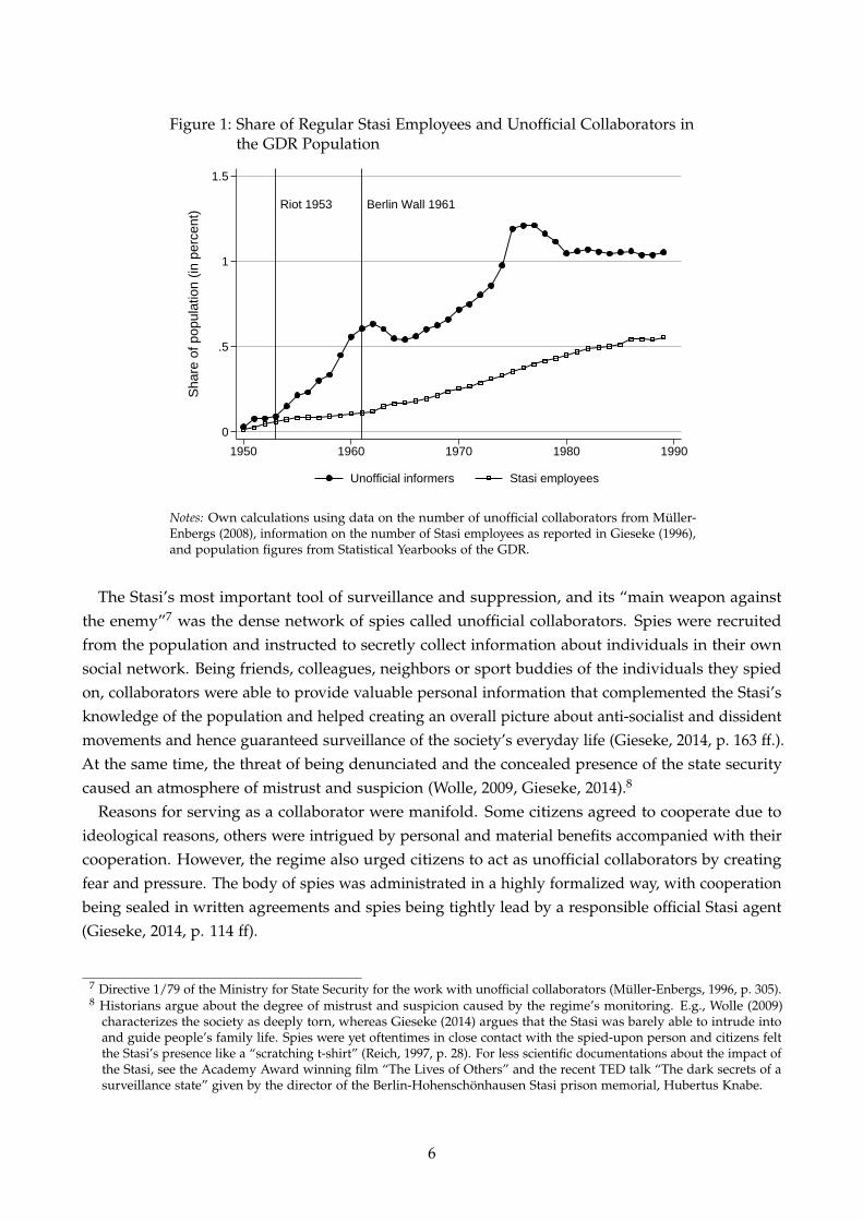
Figure 1: Share of Regular Stasi Employees and Unofficial Collaborators inthe GDR Population

Riot 1953 Berlin Wall 1961

0

.5

1

1.5S

hare

of p

opul

atio

n (in

per

cent

)

1950 1960 1970 1980 1990

Unofficial informers Stasi employees

Notes: Own calculations using data on the number of unofficial collaborators from Muller-Enbergs (2008), information on the number of Stasi employees as reported in Gieseke (1996),and population figures from Statistical Yearbooks of the GDR.

The Stasi’s most important tool of surveillance and suppression, and its “main weapon againstthe enemy”7 was the dense network of spies called unofficial collaborators. Spies were recruitedfrom the population and instructed to secretly collect information about individuals in their ownsocial network. Being friends, colleagues, neighbors or sport buddies of the individuals they spiedon, collaborators were able to provide valuable personal information that complemented the Stasi’sknowledge of the population and helped creating an overall picture about anti-socialist and dissidentmovements and hence guaranteed surveillance of the society’s everyday life (Gieseke, 2014, p. 163 ff.).At the same time, the threat of being denunciated and the concealed presence of the state securitycaused an atmosphere of mistrust and suspicion (Wolle, 2009, Gieseke, 2014).8

Reasons for serving as a collaborator were manifold. Some citizens agreed to cooperate due toideological reasons, others were intrigued by personal and material benefits accompanied with theircooperation. However, the regime also urged citizens to act as unofficial collaborators by creatingfear and pressure. The body of spies was administrated in a highly formalized way, with cooperationbeing sealed in written agreements and spies being tightly lead by a responsible official Stasi agent(Gieseke, 2014, p. 114 ff).

7 Directive 1/79 of the Ministry for State Security for the work with unofficial collaborators (Muller-Enbergs, 1996, p. 305).8 Historians argue about the degree of mistrust and suspicion caused by the regime’s monitoring. E.g., Wolle (2009)

characterizes the society as deeply torn, whereas Gieseke (2014) argues that the Stasi was barely able to intrude intoand guide people’s family life. Spies were yet oftentimes in close contact with the spied-upon person and citizens feltthe Stasi’s presence like a “scratching t-shirt” (Reich, 1997, p. 28). For less scientific documentations about the impact ofthe Stasi, see the Academy Award winning film “The Lives of Others” and the recent TED talk “The dark secrets of asurveillance state” given by the director of the Berlin-Hohenschonhausen Stasi prison memorial, Hubertus Knabe.

6

https://www.ted.com/talks/hubertus_knabe_the_dark_secrets_of_a_surveillance_state

https://www.ted.com/talks/hubertus_knabe_the_dark_secrets_of_a_surveillance_state

3 Data

In this section, we briefly describe the various data sources collected for our empirical analysis.Section 3.1 presents information on our explanatory variable, the spy density in a county. Section 3.2and Section 3.3 describe the data used to construct outcome measures and control variables. Detailedinformation on all variables are provided in Appendix Table B.3. The Data Appendix B also providesdetails on the harmonization of territorial county border changes over time.

3.1 Spy data

Information on the number of spies in each county is based on official Stasi records, published by theAgency of the Federal Commissioner for the Stasi Records (BStU) and compiled in Muller-Enbergs(2008). Although the Stasi was able to destroy part of its files in late 1989, much information waspreserved when protesters started to occupy Stasi offices across the country. In addition, numerousshredded files could be restored after reunification. Since 1991, individual Stasi records are publiclyavailable for personal inspection as well as requests from researchers and the media.

Given that the Stasi saw unofficial collaborators as their main weapon of surveillance, we choosethe county-level share of unofficial collaborators in the population as our main measure of theintensity of surveillance. Most regular Stasi officers were based in the headquarter in Berlin, andonly 10-12 percent of them were employed at the county level. In contrast, the majority of allunofficial collaborators were attached to county offices. The Stasi differentiated between three typesof unofficial collaborators: (i) collaborators for political-operative penetration, homeland defense,or special operations as well as leading informers, (ii) collaborators providing logistics and (iii)societal collaborators, i.e., individuals publicly known as loyal to the state. We use the first categoryof unofficial collaborators to construct our measure of surveillance density, as those were activelyinvolved in spying and are by far the largest and most relevant group of collaborators. If an Object ofSpecial Interest with a separate Stasi office was located in a county, we add the unofficial collaboratorsattached to these object offices to the county’s number of spies.9 As information on the total numberof spies are not given for each year in every county, we use the average share of spies from 1980 to1988 as our measure of surveillance. For further details on our main explanatory variable, see DataAppendix B.

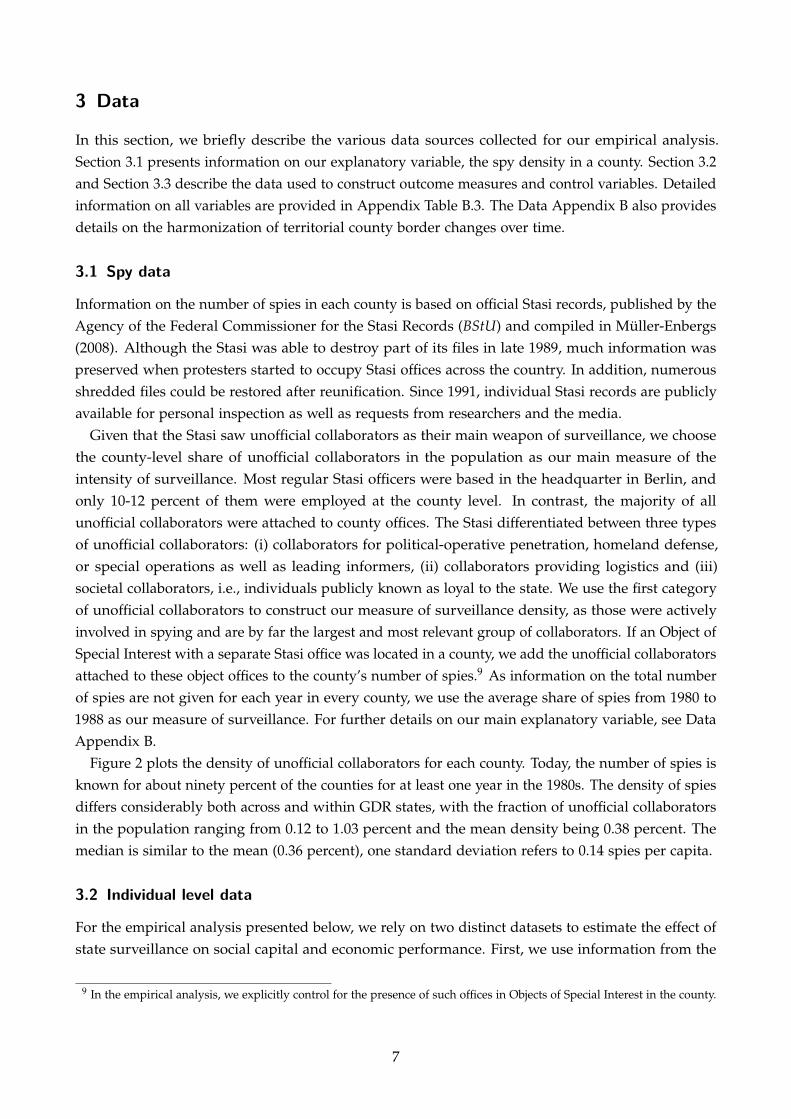
Figure 2 plots the density of unofficial collaborators for each county. Today, the number of spies isknown for about ninety percent of the counties for at least one year in the 1980s. The density of spiesdiffers considerably both across and within GDR states, with the fraction of unofficial collaboratorsin the population ranging from 0.12 to 1.03 percent and the mean density being 0.38 percent. Themedian is similar to the mean (0.36 percent), one standard deviation refers to 0.14 spies per capita.

3.2 Individual level data

For the empirical analysis presented below, we rely on two distinct datasets to estimate the effect ofstate surveillance on social capital and economic performance. First, we use information from the

9 In the empirical analysis, we explicitly control for the presence of such offices in Objects of Special Interest in the county.

7

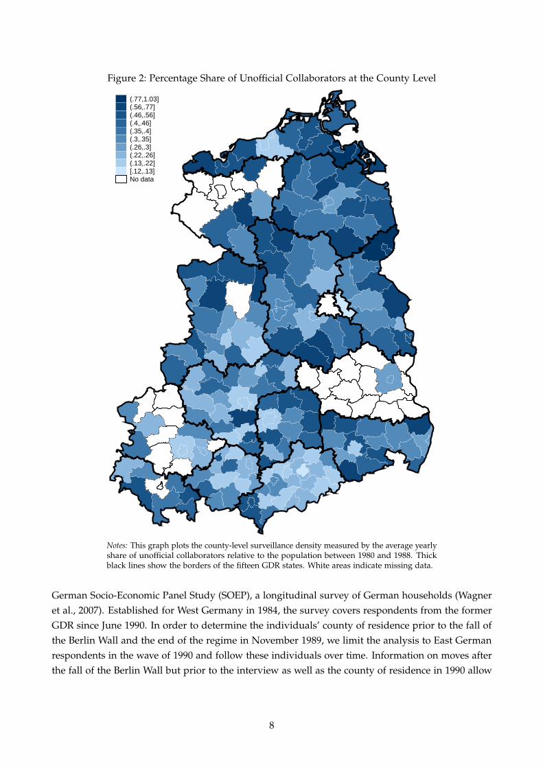
Figure 2: Percentage Share of Unofficial Collaborators at the County Level

(.77,1.03](.56,.77](.46,.56](.4,.46](.35,.4](.3,.35](.26,.3](.22,.26](.13,.22][.12,.13]No data

Notes: This graph plots the county-level surveillance density measured by the average yearlyshare of unofficial collaborators relative to the population between 1980 and 1988. Thickblack lines show the borders of the fifteen GDR states. White areas indicate missing data.

German Socio-Economic Panel Study (SOEP), a longitudinal survey of German households (Wagneret al., 2007). Established for West Germany in 1984, the survey covers respondents from the formerGDR since June 1990. In order to determine the individuals’ county of residence prior to the fall ofthe Berlin Wall and the end of the regime in November 1989, we limit the analysis to East Germanrespondents in the wave of 1990 and follow these individuals over time. Information on moves afterthe fall of the Berlin Wall but prior to the interview as well as the county of residence in 1990 allow

8

us to identify the individuals’ respective counties of residence prior to November 1989. By exploitinga variety of different waves of the survey we are able to observe various measures of social capital aswell as current gross labor income (see Section 4.2 and Data Appendix B).

In order to proxy interpersonal trust, we use two standard measures provided in the SOEP: (i) trustin strangers (see, e.g., Glaeser et al., 2000), and (ii) negative reciprocity (see, e.g., Dohmen et al., 2009).To capture trust in the political system, we investigate two measures as well. First, we take the surveyquestion about the intention to vote if federal elections were held next Sunday. The question capturesthe stated preferences to participate in the most important election. We also use a measure of revealedpreferences, i.e., electoral turnout, below. Second, we exploit the question whether individuals areengaged in local politics. Apart from these variables measuring social capital, we also take reportedmonthly gross labor income as a measure of individual economic performance. Moreover, we usethe rich information of the SOEP to construct a set of individual control variables: gender, age,household size, marital status, level of education and learned profession. For the underlying surveyquestions, data years and exact variable definitions, see Data Appendix B.

3.3 County level data

For the second dataset, we compiled county-level data on various measures of economic performance(self-employment, patents, unemployment, population) as well as electoral turnout as a proxy forsocial capital. We collected county-level data for two time-periods, data from the 1990s and 2000sas well as pre-World War II data. Post-reunification data come from official administrative records;historical data come from various sources (see Data Appendix B for details).

In addition to our outcome variables, we further collect various county-level variables that we useas control variables to check the sensitivity of our estimates. These control variables are used in bothindividual and county level models.

In total, we construct three sets of control variables. The first set measures the strengths of theopposition to the regime. As mentioned in Section 2, the national uprising on and around June 17,1953 constituted the most prominent rebellion against the regime before the large demonstrationsin 1989. The riot markedly changed the regime’s awareness for internal conflicts and triggered theexpansion of the Stasi spy network (cf. Figure 1). We use differences in regional intensity of theriot to proxy the strength of the opposition. Specifically, we construct three control variables: (i) acategorical variable measuring the strike intensity with values “none”, “strike”, “demonstration”,“riot”, and “liberation of prisoners”, (ii) a dummy variable indicating whether the regime declared astate of emergency in the county and (iii) a dummy equal to one if the Soviet military intervened inthe county (for details on the source and the construction of the variables, see Appendix Table B.3).

The second set of controls takes into account that the Stasi tried to protect certain firms in theindustrial sectors. Hence, our industry controls comprise (i) the share of employees in the industrialsector in 1989 and (ii) a dummy variable indicating whether a large enterprise from the uranium,coal, potash, oil or chemical industry was located in the county.

The third set of controls is intended to pick up historical and potentially persistent countydifferences in terms of economic performance and political ideology. It will be used in the modelson the individual level in the absence of pre-treatment information on the outcomes. Our pre World

9

War II controls include (i) the mean share of Nazi and Communist votes in the federal elections of1928, 1930 and the two 1932 elections to capture political extremism (Voigtlander and Voth, 2012), (ii)average electoral turnout in the same elections to proxy institutional trust, (iii) the regional share ofprotestants in 1925 in order to control for differences in work ethic and/or education (Becker andWoßmann, 2009), (iv) the share of self-employed in 1933 to capture regional entrepreneurial spirit and(v) the unemployment rate in 1933 to capture pre-treatment differences in economic performance.

4 Research designs

We present two research designs to identify the causal effect of spying on social capital and economicperformance. First, we lay out a very simple linear model as a benchmark and discuss potentialthreats to identification and likely biases (Section 4.1). Based on this discussion, we propose twoempirical approaches intended to overcome endogeneity problems (Sections 4.2 and 4.3).

4.1 Linear model

To identify the long-term effects of surveillance, we regress various measures of social capital andeconomic performance on our measure of surveillance intensity. The simplest model takes thefollowing form

Yj = α + βSPYDENSc + V ′j ξ + ε j, (1)

where Yj measures an outcome that may either vary at the individual or county level, j ∈ [i, c]. Ourmain regressor is the spy density in county c, defined as the average number of spies per capitain each county of the GDR in the 1980s.10 Vector Vj may contain control variables. In this simplemodel, identification comes from cross-sectional variation in the intensity of surveillance across GDRcounties (see Jacob and Tyrell, 2010, and Friehe et al., 2015, for empirical applications of this model).Two main threats to identification are obvious: (i) selection out of treatment and (ii) omitted variablebias. We discuss these concerns in turn.

Selection out of treatment. If people moved away from counties with a high spying density, wewould face a selection problem that could bias our estimates. However, the authoritarian regimecontrolled and limited external and internal migration in a very strict way, making residential sortinga secondary concern.

First, leaving the East German territory without permission was illegal throughout the existenceof the GDR. Refugees could be sentenced to lengthy terms of imprisonment. However, about threemillion citizens had escaped to West Germany up until the early 1960s, which was the main reasonfor the construction of the Berlin Wall and the expansion of border fortifications in August 1961.Consequently, the large-scale installation of land-mines at the borderland and the regime’s order forsoldiers to shoot at refugees trying to pass the border led to a sharp drop in the number of refugees.The regime also often punished those individuals who applied for emigration visas, exposing people

10 Results do not change when using the density of specific years as a regressor.

10

to considerable harassment in working and private life (Kowalczuk, 2009). Between 1962 and 1988,around 18,000 individuals (0.1 percent of the population) managed to leave East Germany eachyear, either by authorized migration (Ubersiedler) or illegal escape (see Panel (a) in Figure A.1 in theAppendix). The share of refugees on the total number of migrants was around one third and thuseven smaller.

Second, due to considerable housing shortages, residential mobility within the GDR was highlyrestricted. All living space was administered by the GDR authorities: In every municipality, a localhousing agency (Amt fur Wohnungswesen) decided on the allocation of all houses and flats, whetherprivately, cooperatively or publicly owned. Every individual looking for a new apartment hadto file an application at the local housing agency. Processing times often lasted several years andassignment to a new flat was usually subject to economic, political or social interests of the regime(Grashoff, 2011, p. 13f.). From 1975 to 1988, the average number of yearly applications was 755,000,constituting around 4.5 applications per 100 citizens (Steiner, 2006).11 Panel (b) of Figure A.1 in theAppendix shows the extent of residential mobility in the GDR. Mobility of East German citizens hadbeen considerably lower compared to mobility in West Germany. Having data on county populationand the number of spies in multiple years in the 1980s, we can directly test whether the spy densityaffected the population. Reassuringly, we estimate a zero effect of the log number of spies on logpopulation in a model including county and year fixed effects. Hence, selection out of treatmentdoes not seem to be an issue in our setting.

Confounding variables. The second, more serious threat to identification are regional confoundersthat have affected the allocation of Stasi spies in the 1980s and that affect our outcomes of interestafter the fall of the Iron Curtain. Astonishingly, there is very little knowledge on what determinedthe regional spy density. There is some anecdotal evidence that the Stasi was particularly active inregions with strategically important industry clusters. In contrast, and a bit surprisingly, previousresearch could not establish a clear correlation between the size of the Stasi and the size of theopposition at the county level (Gieseke, 1995, p. 190).

Before looking at the effects of spying on social capital and economic outcomes, we try to explainthe regional variation in the spy density, which will be our treatment variable later on. We run asimple OLS regression of the spy density on four sets of potential explanatory variables and checkthe explanatory power of the model as indicated by the R2 measure. Table 1 shows the results,while full regression outputs are shown in Appendix Table A.1. We start off by explaining the spydensity with a constant and a dummy variable, which is equal to one if one of the seven “Objects ofSpecial Interest”, that is, a large public company of strategic importance, was located in the county.12

In the next specification, we add dummy variables for the fifteen GDR states. The R2 measure incolumn (2) shows that around 25 percent of the county-level variation can be explained by differencesacross GDR states. This is suggestive evidence in line with the claim of historians that county offices

11 Some citizens tried to elude the governmental allocation by illegal and unseen movements into dilapidated flats. Thereare no official records about the actual number of illegal squatters. Estimates for the city of Rostock show that the shareof squatters within the population was small, amounting to 0.28 percent in early 1990 (Grashoff, 2011, p. 76).

12 As described in Section 3.1, the Stasi maintained offices in these objects, which recruited their own spies. As we add thespies working in these objects to the number of spies in the respective county offices, we control for “Objects of SpecialInterest” with a dummy variable in all regressions below.

11

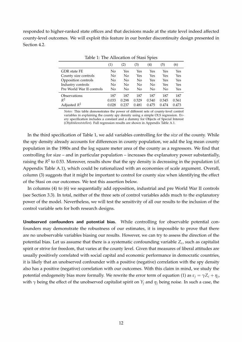
responded to higher-ranked state offices and that decisions made at the state level indeed affectedcounty-level outcomes. We will exploit this feature in our border discontinuity design presented inSection 4.2.

Table 1: The Allocation of Stasi Spies(1) (2) (3) (4) (5) (6)

GDR state FE No Yes Yes Yes Yes YesCounty size controls No No Yes Yes Yes YesOpposition controls No No No Yes Yes YesIndustry controls No No No No Yes YesPre World War II controls No No No No No Yes

Observations 187 187 187 187 187 187R2 0.033 0.298 0.529 0.540 0.545 0.561Adjusted R2 0.028 0.237 0.481 0.475 0.474 0.473

Notes: This table demonstrates the power of different sets of county-level controlvariables in explaining the county spy density using a simple OLS regression. Ev-ery specification includes a constant and a dummy for Objects of Special Interest(Objektdienststellen). Full regression results are shown in Appendix Table A.1.

In the third specification of Table 1, we add variables controlling for the size of the county. Whilethe spy density already accounts for differences in county population, we add the log mean countypopulation in the 1980s and the log square meter area of the county as a regressors. We find thatcontrolling for size – and in particular population – increases the explanatory power substantially,raising the R2 to 0.53. Moreover, results show that the spy density is decreasing in the population (cf.Appendix Table A.1), which could be rationalized with an economies of scale argument. Overall,column (3) suggests that it might be important to control for county size when identifying the effectof the Stasi on our outcomes. We test this assertion below.

In columns (4) to (6) we sequentially add opposition, industrial and pre World War II controls(see Section 3.3). In total, neither of the three sets of control variables adds much to the explanatorypower of the model. Nevertheless, we will test the sensitivity of all our results to the inclusion of thecontrol variable sets for both research designs.

Unobserved confounders and potential bias. While controlling for observable potential con-founders may demonstrate the robustness of our estimates, it is impossible to prove that thereare no unobservable variables biasing our results. However, we can try to assess the direction of thepotential bias. Let us assume that there is a systematic confounding variable Zc, such as capitalistspirit or strive for freedom, that varies at the county level. Given that measures of liberal attitudes areusually positively correlated with social capital and economic performance in democratic countries,it is likely that an unobserved confounder with a positive (negative) correlation with the spy densityalso has a positive (negative) correlation with our outcomes. With this claim in mind, we study thepotential endogeneity bias more formally. We rewrite the error term of equation (1) as ε j = γZc + ηj,with γ being the effect of the unobserved capitalist spirit on Yj and ηj being noise. In such a case, the

12

OLS estimate would be given by:

βOLS =Cov(SPYDENSc, ε j)

Var(SPYDENSc)

= β + γCov(SPYDENSc, Zc)

Var(SPYDENSc)+

Cov(SPYDENSc, ηj)

Var(SPYDENSc)︸︷︷︸=0

.

If, as argued above, the effect of capitalist spirit on the outcome γ and the covariance betweencapitalist spirit and the spying density Cov(SPYDENSc, Zc) have the same sign, and if, as suggestedby the theory of social capital, β < 0, the estimate βOLS will be biased towards zero and underestimatethe negative effect of spying on our outcomes.

In the following subsections, we present two research designs which are intended to better accountfor unobserved confounders and limit the potential endogeneity bias.

4.2 Border discontinuity design

Our first identification strategy exploits the territorial-administrative structure of the Stasi and thefact that about 25 percent of the county-level variation in the spy density can be explained with GDRstate fixed effects (cf. Table 1, column (2)). As the Stasi county offices are subordinate to the stateoffice, different GDR states administered different average levels of spy densities across states. Weuse the resulting discontinuities along state borders as a source of exogenous variation. We followDube et al. (2010) and limit our analysis to all contiguous counties that straddle a GDR state border,thus identifying the effect of spy density on our outcome variables by comparing county pairs oneither side of a state border.13 The identifying assumption is that the county on the lower-spy sideof the border is similar to the county on the higher-spy side in all other relevant characteristics.While such an assumption can be quite strong in similar border research designs, it might be lesscritical in our case given that we focus on post-GDR outcomes and many GDR state borders do notexist anymore. In fact, after reunification the fifteen GDR states merged into six federal states, andaround half of the counties straddling a GDR border in our sample belong to the same federal statein post-reunification Germany.

Formally, we regress individual outcome i in county c, which is part of a border pair b, on the spydensity in county c and border pair dummies νb:

Yicb = α + βSPYDENSc + X ′iδ + K′cφ + νb + ε icb. (2)

As outcome variable, Yicb, we use trust in strangers, extent of negative reciprocity, intention to votein elections, engagement in local politics and individual gross income (see Section 3.2).

The identifying assumption in the border discontinuity design is that counties on either side of aborder differ systematically in their spy density since they belonged to different GDR states. Apartfrom that, there should be no systematic difference between the counties straddling a former state

13 If a county has several direct neighbors on the other side of the state border, we duplicate the observation. See belowfor a discussion.

13

border. However, there might be persistent compositional or historical differences within county-border pairs which affected the spy allocation in the 1980s as well as the post-reunification outcomes.For that reason, we add two sets of control variables as a sensitivity check. First, vector Xi accountsfor compositional differences in the population and includes individual information provided by theSOEP on age, gender, marital status, education and learned profession. Second, vector Kc controlsfor potential county-level differences within a border pair. It is important to understand that in orderto invalidate our research design, these differences must (i) have influenced the spy allocation in the1980s and (ii) affect outcome variables after reunification, making these factors time-persistent perdefinition. As a consequence, we include the county size, opposition, industry and pre-World War IIcontrols that we use above to explain the variation in spy density (cf. Table 1). In addition, we add adummy variable indicating whether an Object of Special Interest was present in the county since weadd the spies attached to this object to the county-level spies (see Sections 3.1 and 4.1).

We use the cross-sectional weights provided by the SOEP to make the sample representative forthe whole population. Given that we duplicate observations in counties that neighbor multiplecounties in a different state, we adjust cross-sectional weights by dividing them through the numberof duplications in our baseline specification and cluster standard errors at the border pair and theindividual level. We test the robustness of our results by (i) disregarding cross-sectional weights andonly accounting for duplications and (ii) by using original cross-sectional weights, not adjusting forduplicates. Results (shown in Appendix Table A.2) prove to be robust to these modifications.

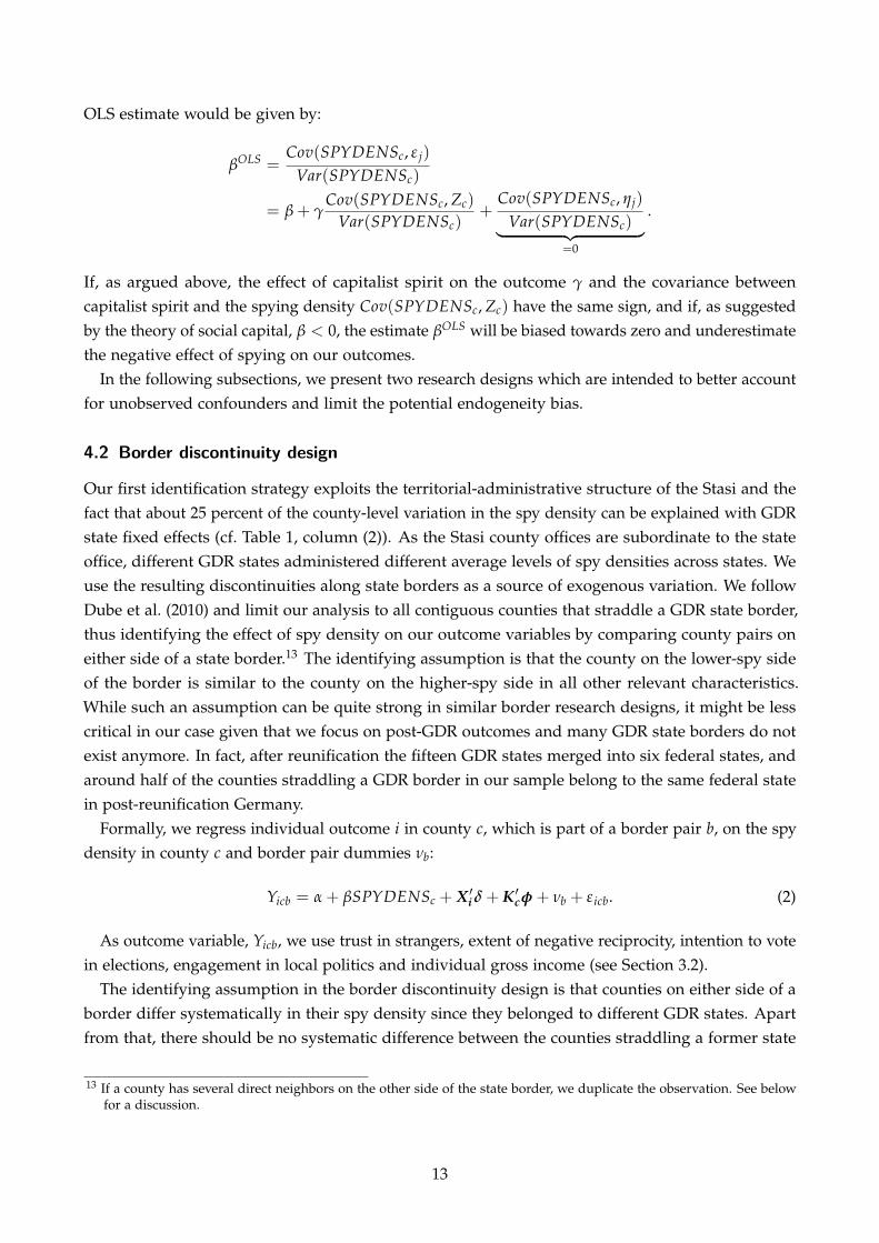
Table 2 provides a test of the validity of our research design by checking whether countiesstraddling a state border are indeed similar. Based on the GDR state average spy density, we assignone county in a border pair to either the higher- or the lower-spy state side. Table 2 shows thedifferences between higher and lower-spying side counties in terms of the spy density and all othercontrol variables used in regression equation (2). We also test whether the differences are statisticallysignificant using a t-test.14 We find that the spy density is indeed significantly higher in countieslocated in higher-spying GDR states. Apart from population, all other control variables seem to bewell balanced between the higher and lower spy density side. The fact that the county population isslightly higher on the lower-spy side is in line with the results from Table A.1: the spy density waslower in cities. For that reason, we control for population and county size in all specifications.

4.3 Panel data design

In Section 4.1, we discussed that time-persistent confounders that have affected the spy allocationand are still affecting post-reunification outcomes are a potential threat to identification. Given thatthe social capital measures obtained from the SOEP are only observed post-treatment, we cannotaccount for these time-persistent potential confounders by including county fixed effects.

However, certain outcomes such as measures of economic performance or political participationcan be observed pre-treatment. Using county-level outcome variables from the late 1920s and early1930s, we apply a panel data research design following Moser et al. (2014) that allows us to includecounty fixed effects to account for any time-invariant confounder.15 The panel data model reads as

14 Note that we use the same weights as in the regression.15 Note that many (though not all) potential confounders are likely to be time-invariant by definition, since they must

14

Table 2: Descriptive Statistics in the Border Pair SampleMean by spy density Difference

Mean SD Low-density High-density ∆ p-value

Spy density 0.36 0.13 0.34 0.38 -0.04 0.04

County variablesLog mean population 1980s 11.14 0.72 11.23 11.04 0.19 0.13Log county size 6.14 0.52 6.10 6.19 -0.10 0.28Dummy: Object of Special Interest 0.03 0.17 0.01 0.04 -0.03 0.31Share indust. employment 1989 45.70 12.15 45.85 45.55 0.30 0.89Dummy: Important industries 1989 0.25 0.44 0.19 0.31 -0.12 0.11Mean electoral turnout 1928–1932 84.10 3.64 83.69 84.52 -0.83 0.19Mean vote share KPD 1928–1932 15.45 6.83 15.71 15.20 0.52 0.66Mean vote share NSDAP 1928–1932 25.36 3.84 25.54 25.17 0.36 0.59Share self-employed 1933 15.75 2.52 15.92 15.57 0.35 0.43Share protestants 1925 91.77 3.85 91.23 92.30 -1.07 0.11Share unemployed 1933 16.80 5.45 17.16 16.44 0.72 0.45Uprising intensity 1953: None 0.29 0.46 0.27 0.31 -0.04 0.57Uprising intensity 1953: Strike 0.25 0.44 0.24 0.27 -0.03 0.69Uprising intensity 1953: Demonstration 0.13 0.34 0.12 0.15 -0.03 0.62Uprising intensity 1953: Riot 0.25 0.43 0.31 0.18 0.13 0.07Uprising intensity 1953: Prisoner liberation 0.07 0.26 0.06 0.09 -0.03 0.51Dummy: State of emergency 1953 0.75 0.43 0.79 0.72 0.07 0.32Dummy: Military intervention 1953 0.57 0.50 0.54 0.60 -0.06 0.49

Individual characteristics (in 1990)Male (in percent) 46.56 49.89 45.89 47.52 -1.64 0.29Age 46.58 18.72 46.75 46.32 0.44 0.80Household size 2.72 1.16 2.67 2.80 -0.13 0.20Share of singles 21.08 40.79 22.66 18.80 3.86 0.23Share of married 59.29 49.13 56.92 62.71 -5.79 0.11Other marital status 19.63 39.72 20.42 18.49 1.94 0.45Share of low-skilled 45.45 49.80 42.92 49.11 -6.19 0.33Share of medium-skilled 34.42 47.52 34.34 34.52 -0.18 0.94Share of high-skilled 20.13 40.10 22.74 16.37 6.36 0.20Learned profession: Blue-collar worker 51.50 49.98 49.41 54.51 -5.10 0.16Learned profession: Self-employed 2.62 15.98 3.24 1.73 1.51 0.15Learned profession: White-collar worker 23.51 42.41 25.08 21.23 3.85 0.35Learned profession: Civil servant 0.25 5.01 0.09 0.49 -0.40 0.25Learned profession: Other/unknown 22.12 41.51 22.18 22.04 0.14 0.96

Notes: The contiguous border pair sample covers 134 counties. Lower-spying and higher-spying counties are determined bymeans of the population-weighted GDR state average of the county-level spy density in the border pair sample. Lower-spyingcounties include 1,131 individuals, higher-spying counties 748 individuals. Descriptive statistics on individual characteristicsare based on the 1990 wave of the SOEP data and calculated using cross-sectional weights, adjusted for duplications of countiesthat are part of multiple border pairs. The corresponding p-values are based on OLS regressions of individual characteristicson an indicator variable for lower-/higher spy density counties, clustering standard errors at the county and person level. Forinformation on all variables, see Appendix Table B.3.

follows:

Yct = α + ∑t

βtSPYDENSc × τt + L′ctζ + ρc + τt + εct. (3)

Outcomes Yct are county c’s election turnout, self-employment rate, number of patents per capita,unemployment rate and log population in year t (see Section 3.3).

have affected the spy allocation in the 1980s and outcomes measure in the 1990s and 2000s.

15

We allow the effect of spying to evolve over time by interacting the time-invariant spy densitySPYDENSc with year dummies τt. Coefficients βt, ∀t ≥ 1989 show the treatment effect afterreunification and demonstrate the potential persistence of the effect. Moreover, coefficients βt, ∀t <1989 provide a direct test of the identifying assumption. If the surveillance levels in the 1980s hadan effect on social capital or economic outcomes prior to fall of the Iron Curtain, this would be anindication that spies were not allocated randomly with respect to the outcome variable. Hence, weneed to have flat, insignificant pre-trends to defend our identifying assumption.16

Year fixed effects τt account for trends in outcome variables over time. In our preferred specification,we even allow for heterogeneous and flexible trends by region (see below). County fixed effectsρc account for persistent confounding variables such as geographic location or regional liberalism.Note that identification in this panel model is somewhat more subtle than in the standard casesince the Stasi density is constant across the panel and identification cannot be within-county as aconsequence. Instead, the model is identified by exploiting cross-sectional variation in post-treatmentadjustment paths. The interactions of the spy density with the year dummies thus capture thepotential relationship between state surveillance in the 1980s and different adjustment paths afterreunification relative to the initial base levels prior to the treatment.

Although we account for county fixed effects, we test the robustness of our results and includeseveral sets of control variables, which are captured in Lct. In a first specification, and as done above,we control for the presence of an Object of Special Interest in county c by interacting a dummyvariable with year dummies after the treatment (t ≥ 1989). Second, we account for both countysize and regional trends. Clearly, rural and urban jurisdiction are likely to show different economicdevelopments in the 1990s and 2000s independent of the Stasi density. The same is true for certainregions. Given that both population and GDR states explain up to 50 percent of the spy densityvariation (cf. Table 1), it is crucial to account for both regional and county-size trends. Concretely, weadd GDR state times year fixed effects to the model17 as well as size controls (log mean populationin the 1980s and log county area) interacted with a dummy indicating the post-treatment period. Inour richest and preferred specification, we also add the opposition and industry controls used inTable (cf. Table 1)—each of them interacted with a post-treatment dummy. Lastly, we apply two othersensitivity checks: First, we add current population to the model, given that it is a potential outcomethat might affect regional adjustment paths. Second, we control for federal and state transfers as wellas investment subsidies paid to East German counties after reunification.

5 Results

In the following section, we present the empirical results. First, we focus on the effect of thespy density on measures of interpersonal and institutional trust (Section 5.1). In Section 5.2, weinvestigate how governmental surveillance affects economic performance. Last, we test the theoretical

16 We omit the spy density for the last pre-treatment year and normalize βt to zero in the respective year. With theexception of the regression for population, our pre-treatment variables are measured prior to World War II. Forunemployment we only observe one pre-treatment year (1933). While this is sufficient to identify county fixed effects,we cannot test for pre-trends regarding regional unemployment in this model specification.

17 For the pre-war periods, we use German states and Prussian provinces from the time of the Weimar Republic.

16

mechanism between government surveillance, social capital, and economic performance using thespy density as an instrument for trust (see Section 5.3).

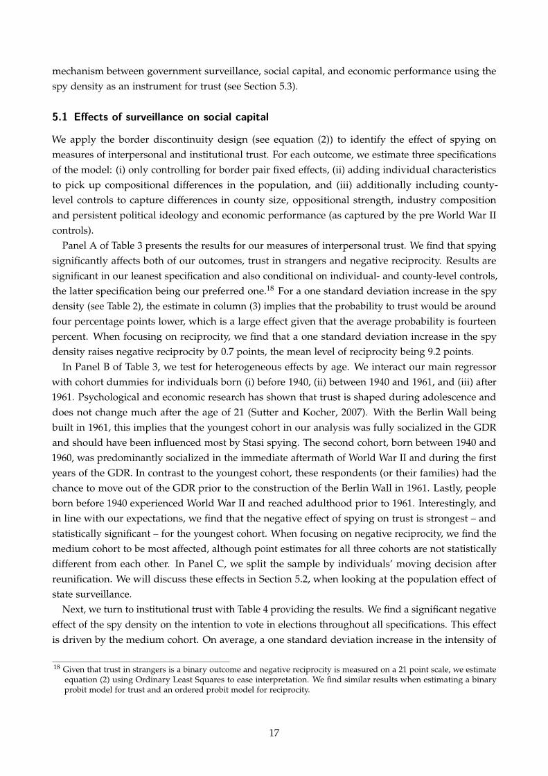
5.1 Effects of surveillance on social capital

We apply the border discontinuity design (see equation (2)) to identify the effect of spying onmeasures of interpersonal and institutional trust. For each outcome, we estimate three specificationsof the model: (i) only controlling for border pair fixed effects, (ii) adding individual characteristicsto pick up compositional differences in the population, and (iii) additionally including county-level controls to capture differences in county size, oppositional strength, industry compositionand persistent political ideology and economic performance (as captured by the pre World War IIcontrols).

Panel A of Table 3 presents the results for our measures of interpersonal trust. We find that spyingsignificantly affects both of our outcomes, trust in strangers and negative reciprocity. Results aresignificant in our leanest specification and also conditional on individual- and county-level controls,the latter specification being our preferred one.18 For a one standard deviation increase in the spydensity (see Table 2), the estimate in column (3) implies that the probability to trust would be aroundfour percentage points lower, which is a large effect given that the average probability is fourteenpercent. When focusing on reciprocity, we find that a one standard deviation increase in the spydensity raises negative reciprocity by 0.7 points, the mean level of reciprocity being 9.2 points.

In Panel B of Table 3, we test for heterogeneous effects by age. We interact our main regressorwith cohort dummies for individuals born (i) before 1940, (ii) between 1940 and 1961, and (iii) after1961. Psychological and economic research has shown that trust is shaped during adolescence anddoes not change much after the age of 21 (Sutter and Kocher, 2007). With the Berlin Wall beingbuilt in 1961, this implies that the youngest cohort in our analysis was fully socialized in the GDRand should have been influenced most by Stasi spying. The second cohort, born between 1940 and1960, was predominantly socialized in the immediate aftermath of World War II and during the firstyears of the GDR. In contrast to the youngest cohort, these respondents (or their families) had thechance to move out of the GDR prior to the construction of the Berlin Wall in 1961. Lastly, peopleborn before 1940 experienced World War II and reached adulthood prior to 1961. Interestingly, andin line with our expectations, we find that the negative effect of spying on trust is strongest – andstatistically significant – for the youngest cohort. When focusing on negative reciprocity, we find themedium cohort to be most affected, although point estimates for all three cohorts are not statisticallydifferent from each other. In Panel C, we split the sample by individuals’ moving decision afterreunification. We will discuss these effects in Section 5.2, when looking at the population effect ofstate surveillance.

Next, we turn to institutional trust with Table 4 providing the results. We find a significant negativeeffect of the spy density on the intention to vote in elections throughout all specifications. This effectis driven by the medium cohort. On average, a one standard deviation increase in the intensity of

18 Given that trust in strangers is a binary outcome and negative reciprocity is measured on a 21 point scale, we estimateequation (2) using Ordinary Least Squares to ease interpretation. We find similar results when estimating a binaryprobit model for trust and an ordered probit model for reciprocity.

17

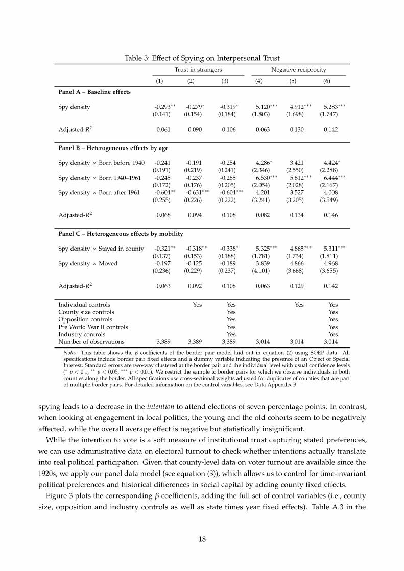
Table 3: Effect of Spying on Interpersonal TrustTrust in strangers Negative reciprocity

(1) (2) (3) (4) (5) (6)

Panel A – Baseline effects

Spy density -0.293∗∗ -0.279∗ -0.319∗ 5.120∗∗∗ 4.912∗∗∗ 5.283∗∗∗

(0.141) (0.154) (0.184) (1.803) (1.698) (1.747)

Adjusted-R2 0.061 0.090 0.106 0.063 0.130 0.142

Panel B – Heterogeneous effects by age

Spy density × Born before 1940 -0.241 -0.191 -0.254 4.286∗ 3.421 4.424∗

(0.191) (0.219) (0.241) (2.346) (2.550) (2.288)Spy density × Born 1940–1961 -0.245 -0.237 -0.285 6.530∗∗∗ 5.812∗∗∗ 6.444∗∗∗

(0.172) (0.176) (0.205) (2.054) (2.028) (2.167)Spy density × Born after 1961 -0.604∗∗ -0.631∗∗∗ -0.604∗∗∗ 4.201 3.527 4.008

(0.255) (0.226) (0.222) (3.241) (3.205) (3.549)

Adjusted-R2 0.068 0.094 0.108 0.082 0.134 0.146

Panel C – Heterogeneous effects by mobility

Spy density × Stayed in county -0.321∗∗ -0.318∗∗ -0.338∗ 5.325∗∗∗ 4.865∗∗∗ 5.311∗∗∗

(0.137) (0.153) (0.188) (1.781) (1.734) (1.811)Spy density × Moved -0.197 -0.125 -0.189 3.839 4.866 4.968

(0.236) (0.229) (0.237) (4.101) (3.668) (3.655)

Adjusted-R2 0.063 0.092 0.108 0.063 0.129 0.142

Individual controls Yes Yes Yes YesCounty size controls Yes YesOpposition controls Yes YesPre World War II controls Yes YesIndustry controls Yes YesNumber of observations 3,389 3,389 3,389 3,014 3,014 3,014

Notes: This table shows the β coefficients of the border pair model laid out in equation (2) using SOEP data. Allspecifications include border pair fixed effects and a dummy variable indicating the presence of an Object of SpecialInterest. Standard errors are two-way clustered at the border pair and the individual level with usual confidence levels(∗ p < 0.1, ∗∗ p < 0.05, ∗∗∗ p < 0.01). We restrict the sample to border pairs for which we observe individuals in bothcounties along the border. All specifications use cross-sectional weights adjusted for duplicates of counties that are partof multiple border pairs. For detailed information on the control variables, see Data Appendix B.

spying leads to a decrease in the intention to attend elections of seven percentage points. In contrast,when looking at engagement in local politics, the young and the old cohorts seem to be negativelyaffected, while the overall average effect is negative but statistically insignificant.

While the intention to vote is a soft measure of institutional trust capturing stated preferences,we can use administrative data on electoral turnout to check whether intentions actually translateinto real political participation. Given that county-level data on voter turnout are available since the1920s, we apply our panel data model (see equation (3)), which allows us to control for time-invariantpolitical preferences and historical differences in social capital by adding county fixed effects.

Figure 3 plots the corresponding β coefficients, adding the full set of control variables (i.e., countysize, opposition and industry controls as well as state times year fixed effects). Table A.3 in the

18

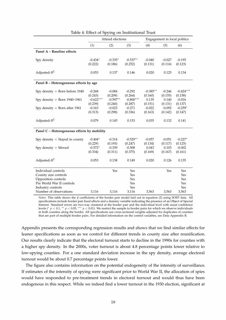
Table 4: Effect of Spying on Institutional TrustAttend elections Engagement in local politics

(1) (2) (3) (4) (5) (6)

Panel A – Baseline effects

Spy density -0.434∗ -0.335∗ -0.537∗∗ -0.040 -0.027 -0.195(0.222) (0.186) (0.252) (0.131) (0.116) (0.123)

Adjusted-R2 0.053 0.137 0.146 0.020 0.125 0.134

Panel B – Heterogeneous effects by age

Spy density × Born before 1940 -0.268 -0.084 -0.292 -0.385∗∗ -0.246 -0.424∗∗∗

(0.243) (0.209) (0.264) (0.160) (0.155) (0.158)Spy density × Born 1940–1961 -0.622∗∗∗ -0.597∗∗ -0.800∗∗∗ 0.135 0.140 -0.016

(0.239) (0.240) (0.287) (0.151) (0.131) (0.137)Spy density × Born after 1961 -0.163 -0.023 -0.271 -0.022 -0.092 -0.259∗

(0.313) (0.298) (0.336) (0.163) (0.142) (0.147)

Adjusted-R2 0.079 0.145 0.153 0.035 0.132 0.141

Panel C – Heterogeneous effects by mobility

Spy density × Stayed in county -0.404∗ -0.314 -0.529∗∗ -0.057 -0.051 -0.227∗

(0.229) (0.193) (0.247) (0.134) (0.117) (0.125)Spy density × Moved -0.572∗ -0.339 -0.508 0.043 0.103 -0.002

(0.334) (0.311) (0.375) (0.169) (0.167) (0.161)

Adjusted-R2 0.053 0.138 0.149 0.020 0.126 0.135

Individual controls Yes Yes Yes YesCounty size controls Yes YesOpposition controls Yes YesPre World War II controls Yes YesIndustry controls Yes YesNumber of observations 3,116 3,116 3,116 3,563 3,563 3,563

Notes: This table shows the β coefficients of the border pair model laid out in equation (2) using SOEP data. Allspecifications include border pair fixed effects and a dummy variable indicating the presence of an Object of SpecialInterest. Standard errors are two-way clustered at the border pair and the individual level with usual confidencelevels (∗ p < 0.1, ∗∗ p < 0.05, ∗∗∗ p < 0.01). We restrict the sample to border pairs for which we observe individualsin both counties along the border. All specifications use cross-sectional weights adjusted for duplicates of countiesthat are part of multiple border pairs. For detailed information on the control variables, see Data Appendix B.

Appendix presents the corresponding regression results and shows that we find similar effects forleaner specifications as soon as we control for different trends in county size after reunification.Our results clearly indicate that the electoral turnout starts to decline in the 1990s for counties witha higher spy density. In the 2000s, voter turnout is about 4.8 percentage points lower relative tolow-spying counties. For a one standard deviation increase in the spy density, average electoralturnout would be about 0.7 percentage points lower.

The figure also contains information on the potential endogeneity of the intensity of surveillance.If estimates of the intensity of spying were significant prior to World War II, the allocation of spieswould have responded to pre-treatment trends in electoral turnout and would thus have beenendogenous in this respect. While we indeed find a lower turnout in the 1930 election, significant at

19

Figure 3: Effect of Spying on Electoral Turnout

-10

-5

0

5

05/1924 1989 1999 2009

Notes: The graph plots the point estimates and corresponding 95 % confidence intervals ofthe spy density interacted with year dummies; see regression model (3). The specificationincludes county fixed effects and state times year fixed effects as well as controls for Objectsof Special Interest, county size, opposition and industry composition. See specification (6)in Table A.3 for details.

the ten percent level, the remaining pre-treatment effects both before and after 1930 are insignificantand small. This suggests that the spy allocation was not systematically determined by pre World WarII trends in institutional trust, which is crucial for establishing causality in our panel model.

5.2 Effects of surveillance on economic performance

Theoretically, we expect government surveillance to deteriorate social capital, which in turn leadsto lower economic performance. While we have demonstrated the first part of this mechanism inthe previous section, we now turn to the economic effects of state surveillance. First, we look at thedirect effect of spying on economic outcomes, hence we estimate reduced form effects.

We begin by analyzing the effect of spying on entrepreneurial activity, given that lacking trustresults in extensive monitoring of “possible malfeasance by partners, employees, and suppliers [and]less time to devote to innovation in new products or processes” (Knack and Keefer, 1997). Indeed,many studies have shown that more trustful people are more likely to become entrepreneurs (Welter,2012, Caliendo et al., 2014). Hence, we consider two outcomes related to entrepreneurial activity,county-level self-employment rates and the number of patents per 100,000 inhabitants.

Figures 4 and 5 plot the respective regression estimates; full regression results are shown inAppendix Tables A.4 and A.5. We find that the self-employment rate is significantly lower (at theten percent level) the higher the county’s spy density. This negative effect is quite persistent andvaries around −2.5 percentage points.19 This estimate implies that for a one standard deviation

19 However, as shown in Appendix Table A.4, we lose precision when including county size controls.

20

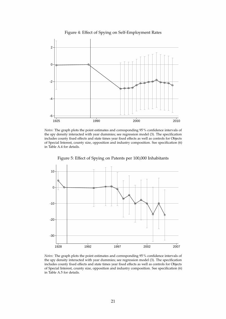
Figure 4: Effect of Spying on Self-Employment Rates

-6

-4

-2

0

2

1925 1990 2000 2010


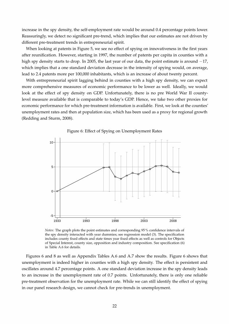
Figure 5: Effect of Spying on Patents per 100,000 Inhabitants

-30

-20

-10

0

10

1928 1992 1997 2002 2007


21

increase in the spy density, the self-employment rate would be around 0.4 percentage points lower.Reassuringly, we detect no significant pre-trend, which implies that our estimates are not driven bydifferent pre-treatment trends in entrepreneurial spirit.

When looking at patents in Figure 5, we see no effect of spying on innovativeness in the first yearsafter reunification. However, starting in 1997, the number of patents per capita in counties with ahigh spy density starts to drop. In 2005, the last year of our data, the point estimate is around −17,which implies that a one standard deviation decrease in the intensity of spying would, on average,lead to 2.4 patents more per 100,000 inhabitants, which is an increase of about twenty percent.

With entrepreneurial spirit lagging behind in counties with a high spy density, we can expectmore comprehensive measures of economic performance to be lower as well. Ideally, we wouldlook at the effect of spy density on GDP. Unfortunately, there is no pre World War II county-level measure available that is comparable to today’s GDP. Hence, we take two other proxies foreconomic performance for which pre-treatment information is available. First, we look at the counties’unemployment rates and then at population size, which has been used as a proxy for regional growth(Redding and Sturm, 2008).

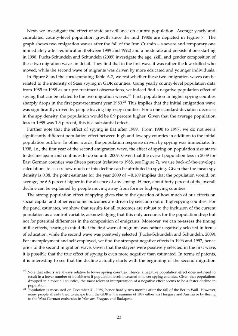
Figure 6: Effect of Spying on Unemployment Rates

-5

0

5

10

1933 1993 1998 2003 2008


Figures 6 and 8 as well as Appendix Tables A.6 and A.7 show the results. Figure 6 shows thatunemployment is indeed higher in counties with a high spy density. The effect is persistent andoscillates around 4.7 percentage points. A one standard deviation increase in the spy density leadsto an increase in the unemployment rate of 0.7 points. Unfortunately, there is only one reliablepre-treatment observation for the unemployment rate. While we can still identify the effect of spyingin our panel research design, we cannot check for pre-trends in unemployment.

22

Next, we investigate the effect of state surveillance on county population. Average yearly andcumulated county-level population growth since the mid 1980s are depicted in Figure 7. Thegraph shows two emigration waves after the fall of the Iron Curtain – a severe and temporary oneimmediately after reunification (between 1989 and 1992) and a moderate and persistent one startingin 1998. Fuchs-Schundeln and Schundeln (2009) investigate the age, skill, and gender composition ofthese two migration waves in detail. They find that in the first wave it was rather the low-skilled whomoved, while the second wave of migrants was driven by more educated and younger individuals.

In Figure 8 and the corresponding Table A.7, we test whether these two emigration waves can berelated to the intensity of Stasi spying in GDR counties. Using yearly county-level population datafrom 1985 to 1988 as our pre-treatment observations, we indeed find a negative population effect ofspying that can be related to the two migration waves.20 First, population in higher spying countiessharply drops in the first post-treatment year 1989.21 This implies that the initial emigration wavewas significantly driven by people leaving high-spy counties. For a one standard deviation decreasein the spy density, the population would be 0.9 percent higher. Given that the average populationloss in 1989 was 1.5 percent, this is a substantial effect.

Further note that the effect of spying is flat after 1989. From 1990 to 1997, we do not see asignificantly different population effect between high and low spy counties in addition to the initialpopulation outflow. In other words, the population response driven by spying was immediate. In1998, i.e., the first year of the second emigration wave, the effect of spying on population size startsto decline again and continues to do so until 2009. Given that the overall population loss in 2009 forEast German counties was fifteen percent (relative to 1988, see Figure 7), we use back-of-the-envelopecalculations to assess how much of this decline can be attributed to spying. Given that the mean spydensity is 0.38, the point estimate for the year 2009 of −0.169 implies that the population would, onaverage, be 6.6 percent higher in the absence of any spying. Hence, about forty percent of the overalldecline can be explained by people moving away from former high-spying counties.

The strong population effect of spying gives rise to the question of how much of our effects onsocial capital and other economic outcomes are driven by selection out of high-spying counties. Forthe panel estimates, we show that results for all outcomes are robust to the inclusion of the currentpopulation as a control variable, acknowledging that this only accounts for the population drop butnot for potential differences in the composition of emigrants. Moreover, we can re-assess the timingof the effects, bearing in mind that the first wave of migrants was rather negatively selected in termsof education, while the second wave was positively selected (Fuchs-Schundeln and Schundeln, 2009).For unemployment and self-employed, we find the strongest negative effects in 1996 and 1997, henceprior to the second migration wave. Given that the stayers were positively selected in the first wave,it is possible that the true effect of spying is even more negative than estimated. In terms of patents,it is interesting to see that the decline actually starts with the beginning of the second migration

20 Note that effects are always relative to lower spying counties. Hence, a negative population effect does not need toresult in a lower number of inhabitants if population levels increased in lower spying counties. Given that populationsdropped in almost all counties, the most relevant interpretation of a negative effect seems to be a faster decline inpopulation.

21 Population is measured on December 31, 1989, hence hardly two months after the fall of the Berlin Wall. However,many people already tried to escape from the GDR in the summer of 1989 either via Hungary and Austria or by fleeingto the West German embassies in Warsaw, Prague, and Budapest.

23

Figure 7: Average County-Level Population Growth in East Germany

November 9, 1989-15

-10

-5

0

Pop

ulat

ion

grow

th (

in p

erce

nt)

1985 1990 1995 2000 2005 2010

Yearly growth Growth relative to 1988

Notes: The graph shows yearly and cumulative average population growth for East Germancounties from 1985 to 2009. Cumulative growth is measured relative to the year 1988.

Figure 8: Effect of Spying on Log Population

-.3

-.2

-.1

0

.1

1985 1990 1995 2000 2005 2010


wave. Hence, it is possible that the effect of spying on patents is of second-order and triggered by theemigration of young and highly educated people.

24

In terms of social capital, we can go a bit further in assessing the potential selection effect. First,note that Table 2 indicates that the initial level in terms of education and learned occupation was notstatistically different between higher and lower spy density counties. Second, we largely estimatethe intention-to-treat effect by assigning individuals the spy density of the county they lived induring the GDR. Unfortunately, we cannot observe individuals who moved to the West in the periodfrom 1989 to June 1990, the month when the 1990 survey was conducted. Given the immediatepopulation response in higher spying counties in 1989, it seems fair to assume that people who movedimmediately after the fall of the Wall (or even before) were particularly affected by spying. Hence,we expect our intention to treat effects of spying on social capital to be slightly underestimated.

As a last robustness check, we interact the spy density with a dummy variable indicating whetherthat individual moved out of the 1989 county of residence; see Panels C of Tables 3 and 4. Ourresults show no significantly different effects between movers and stayers.22 This suggests that thecompositions of movers is not different from stayers in terms of social capital and our findings arenot driven by selection of movers.

Table 5: Effect of Spying on Monthly Gross Labor IncomeReduced form 2SLS

(1) (2) (3) (4) (5)Dependent variable Income Income Income Trust Income

Spy density -1.043∗ -0.776∗ -0.915∗∗ -0.744∗∗∗

(0.560) (0.423) (0.416) (0.245)Trust in strangers 1.354∗

(0.725)

Individual controls Yes Yes Yes YesCounty size controls Yes Yes YesOpposition controls Yes Yes YesPre World War II controls Yes Yes YesIndustry controls Yes Yes Yes

Number of observations 1,773 1,773 1,773 1,743 1,743Adjusted-R2 0.084 0.313 0.341 0.134F-Test 9.237

Notes: This table shows the β coefficients of the border pair model laid out in equation (2) usingSOEP data. All specifications include border pair fixed effects and a dummy variable indicatingthe presence of an Object of Special Interest. Standard errors are two-way clustered at the borderpair and the individual level with usual confidence levels (∗ p < 0.1, ∗∗ p < 0.05, ∗∗∗ p < 0.01).We restrict the sample to border pairs for which we observe individuals in both counties alongthe border. All specifications use cross-sectional weights adjusted for duplicates of counties thatare part of multiple border pairs. For detailed information on the control variables, see DataAppendix B.

5.3 Linking surveillance, social capital and economic performance

In the previous two sections, we provided evidence of negative effects of spying on social capital andeconomic performance. In a last step, we aim at documenting the theoretical mechanism betweengovernment surveillance, social capital, and economic performance. We use gross labor incomereported in the SOEP as our measure of economic performance. First, we estimate the reduced

22 Given that the group of movers is much smaller, we do not obtain statistically significant effects for them.

25

form effect of spying on income (see Table 5, columns (1) to (3)). As expected, we find a negativesignificant effect of the spy density on log gross income of −0.915. The effect implies that a onestandard deviation increase in the spy density leads to a gross income loss of twelve percent. Totest the suggested channel with surveillance affecting trust, and trust affecting income, we run atwo-stage least squares regression of income on trust using the spy density as an instrument. Column(4) of Table 5 shows the first stage result of the regression.23 The F-test of the first-stage regression is9.2, which suggests that the instrument has reasonable power. The second stage results are presentedin column (5). Using the change in trust induced by a one standard deviation decrease in surveillance,the first stage implies a ten percent increase in the probability to trust strangers, which in turnincreases gross income by 15.1 percent.

6 Conclusion

In this paper, we estimate the effect of state mass surveillance on social capital and economicperformance by exploiting county-level variation in the number of spies per capita in the formersocialist German Democratic Republic. To account for the potentially non-random regional allocationof spies, we implement two different research designs. First, we exploit discontinuities at stateborders arising from the administrative territorial structure of the Ministry for State Security, orStasi. For the second research design, we set up a long-term panel with pre World War II measuresof social capital and economic performance. This allows us to control for county fixed effects andidentify the effect of cross-sectional spy density variation through different adjustments paths afterthe breakdown of the regime and the reunification. Moreover, we are able to inspect potentialpre-treatment trends in outcome variables, which would invalidate our identifying assumption.

The results of our analysis show that more intense state surveillance had negative and long-lastingeffects on both social capital and economic performance. Our estimates imply that an abolishmentof all spying activities would have led to an increase in electoral turnout of 1.8 percentage points.Moreover, it would have increased regional innovativeness and entrepreneurship through morepatents per capita and higher self-employment rates. Eventually, the average unemployment ratewould have been about 1.8 percentage points lower, which is equivalent to a ten percent dropcompared to the average in East Germany. We also find that Stasi spying can explain a large partof the decline in population levels in East Germany. Hence, we show that the former East Germanregime did not only have a long-lasting impact on political preferences (Alesina and Fuchs-Schundeln,2007), but it also eroded institutional and interpersonal trust, which in turn has long-lasting negativeeffects on the society and the economy.

23 As found in Table 3, spying has a significantly negative effect on trust. Note that the point estimate is twice as highand more significant despite the smaller sample. This can be explained by the fact the 2SLS sample is restricted toindividuals with positive labor income who are, on average, younger compared to the full estimation sample. In fact,the magnitude of the first-stage estimate is comparable to the one found for the youngest cohort.

26

References

Acemoglu, D., Naidu, S., Restrepo, P. and Robinson, J. A. (2015). Democracy Does Cause Growth.mimeo.

Alesina, A. and Fuchs-Schundeln, N. (2007). Goodbye Lenin (or Not?): The Effect of Communism onPeople’s Preferences, American Economic Review 97(4): 1507–1528.

Algan, Y. and Cahuc, P. (2010). Inherited Trust and Growth, American Economic Review 100(5): 2060–2092.

Arendt, H. (1951). The Origins of Totalitarianism, Harcourt, Brace and Company, New York.

Arrow, K. J. (1972). Gifts and Exchanges, Philosophy & Public Affairs 1(4): 343–362.

Becker, S., Boeckh, K., Hainz, C. and Woßmann, L. (2015). The Empire Is Dead, Long Live theEmpire! Long-Run Persistence of Trust and Corruption in the Bureaucracy, The Economic Journal(forthcoming). doi: 10.1111/ecoj.12220.

Becker, S. O. and Woßmann, L. (2009). Was Weber Wrong? A Human Capital Theory of ProtestantEconomic History, The Quarterly Journal of Economics 124(2): 531–596.

Caliendo, M., Fossen, F. and Kritikos, A. S. (2014). Personality characteristics and the decisions tobecome and stay self-employed, Small Business Economics 42(4): 787–814.

Dohmen, T., Falk, A., Huffman, D. and Sunde, U. (2009). Homo Reciprocans: Survey Evidence OnBehavioural Outcomes, The Economic Journal 119(3): 592–612.

Dube, A., Lester, T. W. and Reich, M. (2010). Minimum wage effects across state borders: Estimatesusing contiguous counties, Review of Economics and Statistics 92(4): 945–964.

Falter, J. W. and Hanisch, D. (1990). Election and Social Data of the Districts and Municipalities ofthe German Empire from 1920 to 1933, GESIS Data Archive, Cologne (ZA8013). doi: 10.4232/1.8013.

Friehe, T., Pannenberg, M. and Wedow, M. (2015). Let Bygones be Bygones? Socialist Regimes andPersonalities in Germany, SOEPpapers 776.

Fuchs-Schundeln, N. and Schundeln, M. (2009). Who stays, who goes, who returns? East – Westmigration within Germany since reunification, Economics of Transition 17: 703–738.

Gieseke, J. (1995). Diskussion, in K.-D. Henke and R. Engelmann (eds), Aktenlage. Die Bedeutungder Unterlagen des Staatssicherheitsdienstes fur die Zeitgeschichtsforschung, Ch. Links Verlag, Berlin,pp. 189–192.

Gieseke, J. (1996). Die hauptamtlichen Mitarbeiter des Ministeriums fur Staatssicherheit (MfS-Handbuch).

Gieseke, J. (2014). The History of the Stasi: East Germany’s Secret Police, 1945–1990, Berghahn Books,New York, Oxford.

27

Glaeser, E. L., Laibson, D. I., Scheinkman, J. A. and Soutter, C. L. (2000). Measuring Trust, TheQuarterly Journal of Economics 115(3): 811–846.

Goodchild, M. F. and Lam, N. S.-N. (1980). Areal Interpolation: A Variant of the Traditional SpatialProblem, Geo-Processing 1: 297–312.

Grashoff, U. (2011). Schwarzwohnen. Die Unterwanderung der staatlichen Wohnraumlenkung in der DDR,V&R unipress, Gottingen.

Guiso, L., Sapienza, P. and Zingales, L. (2006). Does Culture Affect Economic Outcomes?, Journal ofEconomic Perspectives 20(2): 23–48.

Hall, R. E. and Jones, C. I. (1999). Why do Some Countries Produce So Much More Output PerWorker than Others?, The Quarterly Journal of Economics 114(1): 83–116.

Horsch, H. (1997). “Hat nicht wenigstens die Stasi die Stimmung im Lande gekannt?” MfS undSED im Bezirk Karl-Marx-Stadt. Die Entmachtung der Staatssicherheit in den Regionen, Teil 3, BFinformiert 19/1997.

Jacob, M. and Tyrell, M. (2010). The Legacy of Surveillance: An Explanation for Social Capital Erosionand the Persistent Economic Disparity between East and West Germany. mimeo, presented at theSciences Po/IZA Workshop on “Trust, Civic Spirit and Economic Performance” in June 2010.

King, G., Rosen, O., Tanner, M. and Wagner, A. F. (2008). Ordinary Economic Voting Behavior in theExtraordinary Election of Adolf Hitler, The Journal of Economic History 68(4): 951–996.

Knack, S. and Keefer, P. (1997). Does Social Capital Have an Economic Payoff? A Cross-CountryInvestigation, The Quarterly Journal of Economics 112(4): 1251–1288.

Kowalczuk, I.-S. (2009). Endspiel. Die Revolution von 1989 in der DDR, C.H.Beck.

Mauro, P. (1995). Corruption and Growth, The Quarterly Journal of Economics 110(3): 681–712.

Moser, P., Voena, A. and Waldinger, F. (2014). German Jewish Emigres and US Invention, AmericanEconomic Review 104(10): 3222–3255.

Muller-Enbergs, H. (1996). Inoffizielle Mitarbeiter des Ministeriums fur Staatssicherheit. Richtlinien undDurchfuhrungsbestimmungen, Ch. Links Verlag, Berlin.

Muller-Enbergs, H. (2008). Inoffizielle Mitarbeiter des Ministeriums fur Staatssicherheit. Teil 3: Statistik,Ch. Links Verlag, Berlin.

Nunn, N. (2008). The Long-Term Effects of Africa’s Slave Trades, The Quarterly Journal of Economics123(1): 139–176.

Nunn, N. and Wantchekon, L. (2011). The Slave Trade and the Origins of Mistrust in Africa, AmericanEconomic Review 101(7): 3221–3252.

28

Putnam, R. D. (1995). Bowling Alone: America’s Declining Social Capital, Journal of Democracy6(1): 65–78.

Redding, S. J. and Sturm, D. (2008). The Costs of Remoteness: Evidence from German Division andReunification, American Economic Review 98(5): 1766–1797.

Reich, J. (1997). Sicherheit und Feigheit – der Kafer im Brennglas, in S. Suckut (ed.), Staatspartei undStaatssicherheit. Zum Verhaltnis von SED und MfS, Ch. Links Verlag, Berlin, pp. 25–37.

Ritter, J. and Lapp, P. J. (1997). Die Grenze. Ein deutsches Bauwerk, Ch. Links Verlag, Berlin.

Rodrik, D., Subramanian, A. and Trebbi, F. (2004). Institutions Rule: The Primacy of Institutions OverGeography and Integration in Economic Development, Journal of Economic Growth 9(2): 131–165.

Rudolph, H. (1990). Beschaftigungsstrukturen in der DDR vor der Wende, Mitteilungen aus derArbeitsmarkt- und Berufsforschung 4: 474–503.

Ruhle, J. and Holzweißig, G. (1988). Der 13. August 1961. Die Mauer von Berlin, 3 edn, EditionDeutschland Archiv, Koln.

Sobel, J. (2002). Can We Trust Social Capital?, Journal of Economic Literature 40(1): 139–154.

Steiner, A. (2006). Statistische Ubersichten zur Sozialpolitik in Deutschland seit 1945 – BandSBZ/DDR.

Streb, J., Baten, J. and Yin, S. (2006). Technological and geographical knowledge spillover in theGerman empire 1877–1918, Economic History Review LIX(2): 347–373.

Sutter, M. and Kocher, M. G. (2007). Trust and trustworthiness across different age groups, Gamesand Economic Behavior 59(2): 364–382.

Tabellini, G. (2010). Culture and Institutions: Economic Development in the Regions of Europe,Journal of the European Economic Association 8(4): 677–716.

Voigtlander, N. and Voth, H.-J. (2012). Persecution Perpetuated: The Medieval Origins of Anti-SemiticViolence in Nazi Germany, The Quarterly Journal of Economics 127(3): 1339–1392.

Wagner, G. G., Frick, J. R. and Schupp, J. (2007). The German Socio-Economic Panel Study (SOEP):Scope, Evolution and Enhancements, Schmollers Jahrbuch: Journal of Applied Social Science Studies127(1): 139–170.

Welter, F. (2012). All you need is trust? A critical review of the trust and entrepreneurship literature,International Small Business Journal 30(3): 193–212.

Wolf, N. (2009). Was Germany Ever United? Evidence from Intra- and International Trade, 1885–1933,The Journal of Economic History 69(3): 846–881.

Wolle, S. (2009). Die heile Welt der Diktatur. Herrschaft und Alltag in der DDR 1971–1989, Ch. LinksVerlag, Berlin.

29

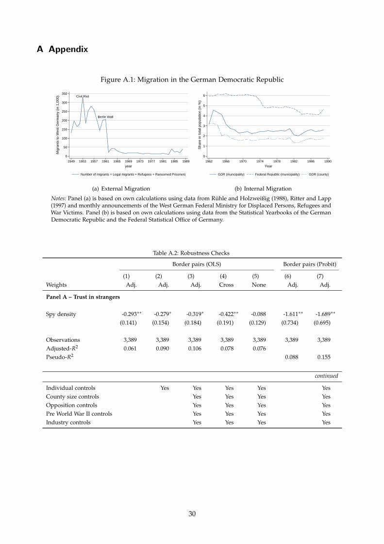
A Appendix

Figure A.1: Migration in the German Democratic Republic

Civil Riot

Berlin Wall

0

50

100

150

200

250

300

350

Mig

rant

s to

Wes

t Ger

man

y (in

1,0

00)

1949 1953 1957 1961 1965 1969 1973 1977 1981 1985 1989

year

Number of migrants = Legal migrants + Refugees + Ransomed Prisoners

(a) External Migration

0

1

2

3

4

5

6

Sha

re in

tota

l pop

ulat

ion

(in %

)

1962 1966 1970 1974 1978 1982 1986 1990

Year

GDR (muncipality) Federal Republic (municipality) GDR (county)

(b) Internal Migration

Notes: Panel (a) is based on own calculations using data from Ruhle and Holzweißig (1988), Ritter and Lapp(1997) and monthly announcements of the West German Federal Ministry for Displaced Persons, Refugees andWar Victims. Panel (b) is based on own calculations using data from the Statistical Yearbooks of the GermanDemocratic Republic and the Federal Statistical Office of Germany.

Table A.2: Robustness Checks

Border pairs (OLS) Border pairs (Probit)

(1) (2) (3) (4) (5) (6) (7)Weights Adj. Adj. Adj. Cross None Adj. Adj.

Panel A – Trust in strangers

Spy density -0.293∗∗ -0.279∗ -0.319∗ -0.422∗∗ -0.088 -1.611∗∗ -1.689∗∗

(0.141) (0.154) (0.184) (0.191) (0.129) (0.734) (0.695)

Observations 3,389 3,389 3,389 3,389 3,389 3,389 3,389Adjusted-R2 0.061 0.090 0.106 0.078 0.076Pseudo-R2 0.088 0.155

continued

Individual controls Yes Yes Yes Yes YesCounty size controls Yes Yes Yes YesOpposition controls Yes Yes Yes YesPre World War II controls Yes Yes Yes YesIndustry controls Yes Yes Yes Yes

30

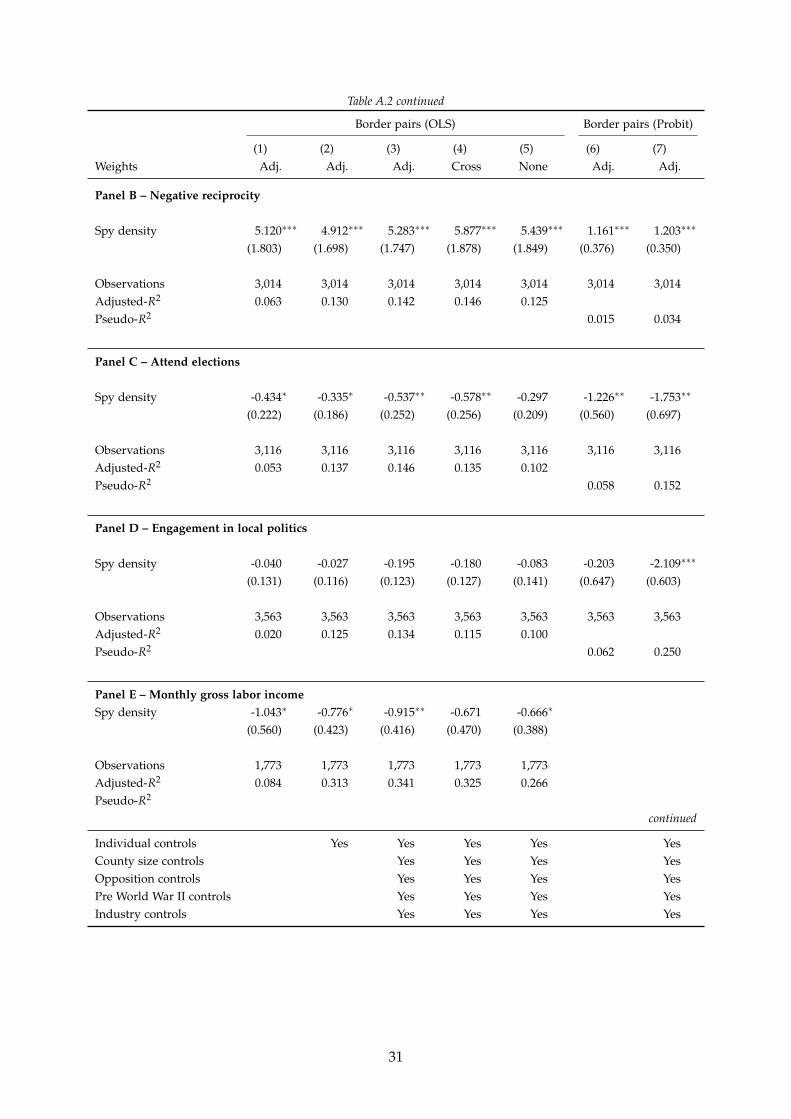
Table A.2 continued



Panel B – Negative reciprocity

Spy density 5.120∗∗∗ 4.912∗∗∗ 5.283∗∗∗ 5.877∗∗∗ 5.439∗∗∗ 1.161∗∗∗ 1.203∗∗∗

(1.803) (1.698) (1.747) (1.878) (1.849) (0.376) (0.350)


Panel C – Attend elections

Spy density -0.434∗ -0.335∗ -0.537∗∗ -0.578∗∗ -0.297 -1.226∗∗ -1.753∗∗

(0.222) (0.186) (0.252) (0.256) (0.209) (0.560) (0.697)


Panel D – Engagement in local politics

Spy density -0.040 -0.027 -0.195 -0.180 -0.083 -0.203 -2.109∗∗∗

(0.131) (0.116) (0.123) (0.127) (0.141) (0.647) (0.603)


Panel E – Monthly gross labor incomeSpy density -1.043∗ -0.776∗ -0.915∗∗ -0.671 -0.666∗

(0.560) (0.423) (0.416) (0.470) (0.388)

Observations 1,773 1,773 1,773 1,773 1,773Adjusted-R2 0.084 0.313 0.341 0.325 0.266Pseudo-R2

continued


31

Table A.2 continued




Notes: This table shows the β coefficients of the border pair model laid out in equation (2) using SOEP data. Allspecifications include border pair fixed effects and a dummy variable indicating the presence of an Object ofSpecial Interest. Standard errors are two-way clustered at the border pair and the individual level in specifications(1)-(5) and one-way clustered at the border pair level only in specifications (6)-(7). We use the usual confidencelevels (∗ p < 0.1, ∗∗ p < 0.05, ∗∗∗ p < 0.01). We restrict the sample to border pairs for which we observe individualsin both counties along the border. Columns (1)-(3) and (6)-(7) present estimates using cross-sectional weights,adjusted for duplications of counties that are part of multiple border pairs. Estimates in column (4) use unadjustedcross-sectional weights, column (5) shows unweighted regression results but adjusts for duplicates. Specifications(6)-(7) present ordered probit results if negative reciprocity is the outcome variable. For detailed information onthe control variables, see Data Appendix B.

32

Table A.1: The Allocation of Stasi Spies – Full Regression Results(1) (2) (3) (4) (5) (6)

Dummy: Object of Special Interest 0.160 0.172 0.261∗∗∗ 0.267∗∗∗ 0.265∗∗∗ 0.272∗∗∗

(0.124) (0.114) (0.067) (0.069) (0.070) (0.076)Log mean population 1980s -0.134∗∗∗ -0.144∗∗∗ -0.148∗∗∗ -0.135∗∗∗

(0.015) (0.016) (0.016) (0.021)Log county size -0.006 -0.002 0.001 0.003

(0.011) (0.012) (0.012) (0.014)Uprising intensity 1953: Strike 0.004 -0.001 -0.005

(0.024) (0.026) (0.027)Uprising intensity 1953: Demonstration 0.002 -0.006 -0.014

(0.026) (0.027) (0.031)Uprising intensity 1953: Riot -0.030 -0.035 -0.041

(0.037) (0.038) (0.038)Uprising intensity 1953: Prisoner liberation 0.002 -0.005 -0.015

(0.034) (0.035) (0.038)Dummy: Military intervention 1953 0.037 0.037 0.045∗

(0.023) (0.023) (0.024)Dummy: State of emergency 1953 -0.014 -0.009 -0.009

(0.026) (0.027) (0.029)Share indust. employment 1989 0.001 0.001

(0.001) (0.001)Dummy: Important industries 1989 -0.003 -0.011

(0.022) (0.022)Mean electoral turnout 1928–1932 0.001

(0.006)Mean vote share NSDAP 1928–1932 0.006∗∗

(0.003)Mean vote share KPD 1928–1932 -0.000

(0.003)Share protestants 1925 -0.001

(0.001)Share unemployed 1933 0.001

(0.004)Share self-employed 1933 0.004

(0.009)GDR state FE No Yes Yes Yes Yes Yes

Observations 187 187 187 187 187 187R2 0.033 0.298 0.529 0.540 0.545 0.561Adjusted R2 0.028 0.237 0.481 0.475 0.474 0.473

Notes: This table shows the simple OLS coefficients of regressing the mean county-level spy density in the 1980s on differentsets of control variables. For details on the source and construction of the variables, see Appendix Table B.3.

33

Table A.3: Effect of Spying on Electoral Turnout(1) (2) (3) (4) (5) (6) (7) (8)

Spy density × 05/1924 0.327 0.327 0.327 -1.305 -1.305 -1.305 -1.343 -1.305(1.513) (1.515) (1.516) (1.460) (1.462) (1.463) (1.453) (1.462)

Spy density × 12/1924 0.341 0.341 0.341 -0.972 -0.972 -0.972 -1.022 -0.972(1.418) (1.420) (1.421) (1.452) (1.454) (1.455) (1.442) (1.454)

Spy density × 1928 2.316 2.316 2.316 0.354 0.354 0.354 0.357 0.354(1.659) (1.661) (1.662) (1.581) (1.583) (1.584) (1.584) (1.583)

Spy density × 1930 -2.379∗ -2.379∗ -2.379∗ -2.192∗ -2.192∗ -2.192∗ -2.183∗ -2.192∗

(1.217) (1.219) (1.219) (1.164) (1.166) (1.166) (1.166) (1.165)Spy density × 07/1932 -0.479 -0.479 -0.479 -0.239 -0.239 -0.239 -0.231 -0.239

(0.809) (0.811) (0.811) (0.580) (0.580) (0.581) (0.581) (0.580)Spy density × 1990 -2.367 -1.888 -5.534∗∗ -0.554 -0.745 -0.480 -0.510

(2.290) (2.340) (2.647) (2.101) (2.166) (2.162) (2.166)Spy density × 1994 -2.753 -2.894 -6.540∗∗ -2.710 -2.901 -2.635 -2.667

(2.298) (2.340) (2.740) (2.212) (2.278) (2.256) (2.223)Spy density × 1998 -6.205∗∗∗ -6.505∗∗∗ -10.151∗∗∗ -1.585 -1.776 -1.511 -1.558 -0.866

(2.228) (2.202) (2.640) (1.975) (2.037) (2.036) (2.072) (2.071)Spy density × 2002 0.638 0.963 -2.683 -3.988∗ -4.179∗∗ -3.914∗ -3.919∗ -3.082

(2.109) (2.170) (2.641) (2.041) (2.092) (2.086) (2.047) (2.087)Spy density × 2005 0.167 0.500 -3.147 -3.726∗ -3.917∗ -3.652∗ -3.592∗ -2.643

(1.993) (2.053) (2.513) (2.067) (2.124) (2.134) (2.038) (2.166)Spy density × 2009 2.666 2.924 -0.723 -4.878∗∗ -5.069∗∗ -4.804∗∗ -4.644∗∗ -2.971

(2.264) (2.335) (2.779) (2.190) (2.268) (2.269) (2.201) (2.273)

Post × Object of SI x Year FE Yes Yes Yes Yes Yes Yes YesPost × County size controls Yes Yes Yes Yes Yes YesState × Year FE Yes Yes Yes Yes YesPost × Opposition controls Yes Yes Yes YesPost × Industry controls Yes Yes YesLog current population YesPost × Transfers Yes

Observations 2232 2232 2232 2232 2232 2232 2230 1858Adjusted R2 0.826 0.826 0.829 0.919 0.920 0.921 0.923 0.930

Notes: This table shows the β coefficients of the panel data model laid out in equation (3). All specifications include district and year fixedeffects. Standard errors are clustered at the district level with the usual confidence levels (∗ p < .1, ∗∗ p < .05, ∗∗∗ p < .01). The Stasishare-year interaction for November 1932 is omitted. The district of East Berlin is excluded from the data because East and West Berlincannot be separated after reunification. Post is a dummy for the period after the fall of the Berlin Wall (t ≥ 1989). Object of SI stands forObject of Special Interest. County size controls include log county area and log mean 1980s population. State refers to GDR states in the1980s and post-reunification, and to Weimar provinces prior to World War II. For detailed information on the control variables, see DataAppendix B.

34

Table A.4: Effect of Spying on Self-Employment Rates(1) (2) (3) (4) (5) (6) (7) (8)

Spy density × 1925 -1.353 -1.353 -1.353 -0.083 -0.083 -0.083 0.023 -0.083(1.326) (1.330) (1.330) (1.437) (1.439) (1.439) (1.441) (1.440)

Spy density × 1996 -3.694∗∗∗ -4.155∗∗∗ -2.938∗ -2.188 -2.468 -2.837∗ -2.769∗ -2.773∗

(1.220) (1.117) (1.512) (1.455) (1.517) (1.540) (1.421) (1.532)Spy density × 1997 -3.751∗∗∗ -4.197∗∗∗ -2.979∗ -2.132 -2.412 -2.782∗ -2.708∗ -2.733∗

(1.259) (1.164) (1.558) (1.485) (1.544) (1.565) (1.454) (1.557)Spy density × 1998 -3.626∗∗∗ -4.061∗∗∗ -2.843∗ -2.125 -2.405 -2.774∗ -2.704∗ -2.755∗

(1.259) (1.170) (1.571) (1.479) (1.536) (1.557) (1.453) (1.556)Spy density × 1999 -3.534∗∗∗ -3.949∗∗∗ -2.731∗ -2.070 -2.349 -2.719∗ -2.652∗ -2.705∗

(1.264) (1.203) (1.607) (1.474) (1.529) (1.545) (1.445) (1.541)Spy density × 2000 -3.504∗∗∗ -3.914∗∗∗ -2.697 -1.777 -2.056 -2.426 -2.366 -2.433

(1.294) (1.229) (1.633) (1.460) (1.517) (1.538) (1.437) (1.532)Spy density × 2001 -3.060∗∗ -3.431∗∗∗ -2.213 -1.546 -1.826 -2.196 -2.145 -2.218

(1.301) (1.234) (1.633) (1.489) (1.545) (1.565) (1.469) (1.558)Spy density × 2002 -2.973∗∗ -3.332∗∗∗ -2.115 -1.523 -1.803 -2.173 -2.133 -2.160

(1.320) (1.241) (1.629) (1.493) (1.547) (1.567) (1.477) (1.555)Spy density × 2003 -2.859∗∗ -3.214∗∗ -1.996 -1.399 -1.678 -2.048 -2.022 -2.041

(1.366) (1.286) (1.669) (1.528) (1.582) (1.599) (1.513) (1.594)Spy density × 2004 -2.851∗∗ -3.213∗∗ -1.995 -1.355 -1.635 -2.004 -1.992 -1.946

(1.397) (1.317) (1.691) (1.541) (1.597) (1.614) (1.526) (1.600)Spy density × 2005 -2.475∗ -2.779∗∗ -1.562 -1.154 -1.434 -1.804 -1.810 -1.728

(1.407) (1.348) (1.716) (1.558) (1.611) (1.625) (1.540) (1.614)Spy density × 2006 -2.799∗∗ -3.086∗∗ -1.868 -1.434 -1.714 -2.083 -2.107 -2.021

(1.416) (1.354) (1.715) (1.571) (1.620) (1.635) (1.558) (1.627)Spy density × 2007 -2.623∗ -2.935∗∗ -1.717 -1.494 -1.774 -2.143 -2.184 -2.132

(1.397) (1.311) (1.676) (1.562) (1.612) (1.630) (1.560) (1.619)Spy density × 2008 -2.305∗ -2.560∗∗ -1.342 -1.542 -1.822 -2.192 -2.251 -2.186

(1.354) (1.297) (1.668) (1.542) (1.593) (1.611) (1.539) (1.601)Spy density × 2009 -2.248∗ -2.484∗ -1.266 -1.781 -2.061 -2.430 -2.507 -2.413

(1.348) (1.299) (1.676) (1.539) (1.593) (1.611) (1.541) (1.612)



Notes: This table shows the β coefficients of the panel data model laid out in equation (3). All specifications include district andyear fixed effects. Standard errors are clustered at the district level with the usual confidence levels (∗ p < .1, ∗∗ p < .05, ∗∗∗

p < .01). The Stasi share-year interaction for 1933 is omitted. The district of East Berlin is excluded from the data because Eastand West Berlin cannot be separated after reunification. Post is a dummy for the period after the fall of the Berlin Wall (t ≥ 1989).Object of SI stands for Object of Special Interest. County size controls include log county area and log mean 1980s population. Staterefers to GDR states in the 1980s and post-reunification, and to Weimar provinces prior to World War II. For detailed informationon the control variables, see Data Appendix B.

35

Table A.5: Effect of Spying on Patents per 100,000 Inhabitants(1) (2) (3) (4) (5) (6) (7) (8)

Spy density × 1928 3.685∗ 3.685∗ 3.685∗ 4.285 4.285 4.285 4.289 4.285(1.947) (1.952) (1.953) (2.887) (2.891) (2.892) (2.895) (2.893)

Spy density × 1993 -5.397 -4.891 -0.411 -2.008 -0.966 -0.373 -0.396(3.968) (4.463) (5.511) (5.898) (5.834) (5.850) (6.050)

Spy density × 1995 -5.673 -3.361 1.118 -1.118 -0.076 0.516 0.507 0.714(3.930) (5.416) (5.857) (6.659) (6.296) (6.051) (6.132) (6.097)

Spy density × 1996 -6.545 -5.109 -0.629 -0.958 0.084 0.677 0.678 0.519(4.366) (5.668) (6.146) (6.825) (6.446) (6.228) (6.340) (6.302)

Spy density × 1997 -6.956∗ -6.052 -1.572 -2.673 -1.631 -1.038 -1.029 -1.134(4.074) (5.128) (5.462) (5.722) (5.411) (5.249) (5.378) (5.332)

Spy density × 1998 -13.326∗∗∗ -13.433∗∗ -8.954 -8.741 -7.699 -7.106 -7.102 -7.578(4.577) (5.471) (6.239) (6.380) (5.974) (5.722) (5.803) (5.678)

Spy density × 1999 -9.876∗∗ -9.350 -4.870 -6.416 -5.374 -4.781 -4.782 -5.261(4.725) (5.848) (6.576) (6.708) (6.284) (6.061) (6.183) (6.036)

Spy density × 2000 -13.226∗∗∗ -13.858∗∗ -9.378 -11.724∗ -10.682∗ -10.089∗ -10.102∗ -10.335∗

(5.032) (5.862) (6.603) (6.572) (6.052) (5.833) (5.925) (5.832)Spy density × 2001 -9.948∗ -10.716 -6.236 -9.451 -8.409 -7.816 -7.846 -7.741

(5.593) (6.538) (7.167) (6.868) (6.515) (6.327) (6.456) (6.282)Spy density × 2002 -10.802 -13.265∗ -8.785 -11.676 -10.633 -10.041 -10.088 -9.837

(6.556) (7.870) (8.427) (8.366) (7.911) (7.681) (7.751) (7.561)Spy density × 2003 -15.861∗∗ -18.940∗∗ -14.460∗ -18.417∗ -17.375∗ -16.782∗ -16.852∗ -16.317∗

(6.109) (8.013) (8.282) (9.498) (8.928) (8.560) (8.602) (8.391)Spy density × 2004 -9.422 -12.959 -8.479 -11.568 -10.526 -9.934 -10.027 -9.194

(6.665) (7.905) (8.410) (8.674) (8.220) (7.984) (8.091) (7.935)Spy density × 2005 -10.239 -15.291∗ -10.811 -18.778∗∗ -17.736∗∗ -17.143∗∗ -17.267∗∗ -16.280∗∗

(6.992) (8.377) (8.877) (8.548) (8.114) (7.921) (7.987) (7.855)



Notes: This table shows the β coefficients of the panel data model laid out in equation (3). All specifications include district and year fixedeffects. Standard errors are clustered at the district level with the usual confidence levels (∗ p < .1, ∗∗ p < .05, ∗∗∗ p < .01). The Stasishare-year interaction for 1929 is omitted. The district of East Berlin is excluded from the data because East and West Berlin cannot beseparated after reunification. Post is a dummy for the period after the fall of the Berlin Wall (t ≥ 1989). Object of SI stands for Object ofSpecial Interest. County size controls include log county area and log mean 1980s population. State refers to GDR states in the 1980s andpost-reunification, and to Weimar provinces prior to World War II. For detailed information on the control variables, see Data Appendix B.

36

Table A.6: Effect of Spying on Unemployment Rates(1) (2) (3) (4) (5) (6) (7) (8)

Spy density × 1996 19.852∗∗∗ 21.075∗∗∗ 10.195∗∗∗ 4.287∗ 4.734∗ 4.838∗ 4.741∗∗ 4.916∗∗

(3.054) (3.016) (3.296) (2.453) (2.510) (2.466) (2.327) (2.465)Spy density × 1997 19.187∗∗∗ 20.269∗∗∗ 9.388∗∗∗ 4.377∗ 4.824∗ 4.928∗ 4.822∗∗ 4.990∗∗

(3.071) (3.058) (3.303) (2.515) (2.564) (2.524) (2.387) (2.517)Spy density × 1998 18.163∗∗∗ 19.101∗∗∗ 8.220∗∗ 2.440 2.887 2.991 2.891 3.042

(2.988) (2.940) (3.242) (2.448) (2.494) (2.465) (2.315) (2.461)Spy density × 1999 18.245∗∗∗ 19.261∗∗∗ 8.380∗∗∗ 1.977 2.424 2.528 2.433 2.574

(2.891) (2.825) (3.189) (2.345) (2.409) (2.379) (2.223) (2.377)Spy density × 2000 19.055∗∗∗ 20.078∗∗∗ 9.197∗∗∗ 2.650 3.097 3.202 3.119 3.221

(2.895) (2.827) (3.215) (2.379) (2.451) (2.423) (2.279) (2.418)Spy density × 2001 19.968∗∗∗ 21.204∗∗∗ 10.324∗∗∗ 3.188 3.635 3.739 3.675 3.734

(2.916) (2.825) (3.193) (2.416) (2.496) (2.464) (2.335) (2.466)Spy density × 2002 19.610∗∗∗ 20.811∗∗∗ 9.931∗∗∗ 2.932 3.379 3.483 3.438 3.504

(2.893) (2.841) (3.185) (2.459) (2.544) (2.515) (2.367) (2.519)Spy density × 2003 21.232∗∗∗ 22.497∗∗∗ 11.617∗∗∗ 3.529 3.976 4.081 4.061 4.086

(3.121) (3.081) (3.397) (2.586) (2.660) (2.629) (2.506) (2.629)Spy density × 2004 22.038∗∗∗ 23.330∗∗∗ 12.450∗∗∗ 3.975 4.422 4.526∗ 4.531∗ 4.567∗

(3.154) (3.137) (3.458) (2.655) (2.732) (2.704) (2.584) (2.701)Spy density × 2005 21.394∗∗∗ 22.625∗∗∗ 11.744∗∗∗ 4.584∗ 5.031∗ 5.136∗ 5.175∗∗ 5.187∗

(2.926) (2.999) (3.357) (2.585) (2.674) (2.648) (2.528) (2.638)Spy density × 2006 21.777∗∗∗ 23.246∗∗∗ 12.366∗∗∗ 4.719∗ 5.166∗ 5.270∗ 5.342∗∗ 5.298∗∗

(3.014) (2.972) (3.381) (2.642) (2.714) (2.689) (2.594) (2.683)Spy density × 2007 21.949∗∗∗ 23.237∗∗∗ 12.357∗∗∗ 4.504∗ 4.951∗ 5.055∗ 5.159∗ 5.025∗

(2.971) (2.927) (3.379) (2.670) (2.743) (2.722) (2.626) (2.727)Spy density × 2008 20.640∗∗∗ 21.914∗∗∗ 11.034∗∗∗ 3.448 3.895 3.999 4.138∗ 3.969

(2.872) (2.766) (3.249) (2.494) (2.574) (2.553) (2.447) (2.561)Spy density × 2009 19.308∗∗∗ 20.537∗∗∗ 9.657∗∗∗ 3.264 3.711 3.816 3.985∗ 3.916

(2.727) (2.653) (3.118) (2.460) (2.547) (2.523) (2.404) (2.531)



Notes: This table shows the β coefficients of the panel data model laid out in equation (3). All specifications include district and yearfixed effects. Standard errors are clustered at the district level with the usual confidence levels (∗ p < .1, ∗∗ p < .05, ∗∗∗ p < .01). The Stasishare-year interaction for 1933 is omitted. The district of East Berlin is excluded from the data because East and West Berlin cannot beseparated after reunification. Post is a dummy for the period after the fall of the Berlin Wall (t ≥ 1989). Object of SI stands for Object ofSpecial Interest. County size controls include log county area and log mean 1980s population. State refers to GDR states in the 1980s andpost-reunification, and to Weimar provinces prior to World War II. For detailed information on the control variables, see Data AppendixB.

37

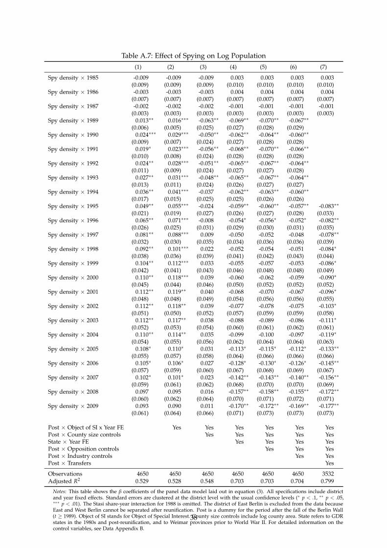
Table A.7: Effect of Spying on Log Population(1) (2) (3) (4) (5) (6) (7)

Spy density × 1985 -0.009 -0.009 -0.009 0.003 0.003 0.003 0.003(0.009) (0.009) (0.009) (0.010) (0.010) (0.010) (0.010)

Spy density × 1986 -0.003 -0.003 -0.003 0.004 0.004 0.004 0.004(0.007) (0.007) (0.007) (0.007) (0.007) (0.007) (0.007)

Spy density × 1987 -0.002 -0.002 -0.002 -0.001 -0.001 -0.001 -0.001(0.003) (0.003) (0.003) (0.003) (0.003) (0.003) (0.003)

Spy density × 1989 0.013∗∗ 0.016∗∗∗ -0.063∗∗ -0.069∗∗ -0.070∗∗ -0.067∗∗

(0.006) (0.005) (0.025) (0.027) (0.028) (0.029)Spy density × 1990 0.024∗∗∗ 0.029∗∗∗ -0.050∗∗ -0.062∗∗ -0.064∗∗ -0.060∗∗

(0.009) (0.007) (0.024) (0.027) (0.028) (0.028)Spy density × 1991 0.019∗ 0.023∗∗∗ -0.056∗∗ -0.068∗∗ -0.070∗∗ -0.066∗∗

(0.010) (0.008) (0.024) (0.028) (0.028) (0.028)Spy density × 1992 0.024∗∗ 0.028∗∗∗ -0.051∗∗ -0.065∗∗ -0.067∗∗ -0.064∗∗

(0.011) (0.009) (0.024) (0.027) (0.027) (0.028)Spy density × 1993 0.027∗∗ 0.031∗∗∗ -0.048∗∗ -0.065∗∗ -0.067∗∗ -0.064∗∗

(0.013) (0.011) (0.024) (0.026) (0.027) (0.027)Spy density × 1994 0.036∗∗ 0.041∗∗∗ -0.037 -0.062∗∗ -0.063∗∗ -0.060∗∗

(0.017) (0.015) (0.025) (0.025) (0.026) (0.026)Spy density × 1995 0.049∗∗ 0.055∗∗∗ -0.024 -0.059∗∗ -0.060∗∗ -0.057∗∗ -0.083∗∗

(0.021) (0.019) (0.027) (0.026) (0.027) (0.028) (0.033)Spy density × 1996 0.065∗∗ 0.071∗∗∗ -0.008 -0.054∗ -0.056∗ -0.052∗ -0.082∗∗

(0.026) (0.025) (0.031) (0.029) (0.030) (0.031) (0.035)Spy density × 1997 0.081∗∗ 0.088∗∗∗ 0.009 -0.050 -0.052 -0.048 -0.078∗∗

(0.032) (0.030) (0.035) (0.034) (0.036) (0.036) (0.039)Spy density × 1998 0.092∗∗ 0.101∗∗∗ 0.022 -0.052 -0.054 -0.051 -0.084∗

(0.038) (0.036) (0.039) (0.041) (0.042) (0.043) (0.044)Spy density × 1999 0.104∗∗ 0.112∗∗∗ 0.033 -0.055 -0.057 -0.053 -0.086∗

(0.042) (0.041) (0.043) (0.046) (0.048) (0.048) (0.049)Spy density × 2000 0.110∗∗ 0.118∗∗∗ 0.039 -0.060 -0.062 -0.059 -0.090∗

(0.045) (0.044) (0.046) (0.050) (0.052) (0.052) (0.052)Spy density × 2001 0.112∗∗ 0.119∗∗ 0.040 -0.068 -0.070 -0.067 -0.096∗

(0.048) (0.048) (0.049) (0.054) (0.056) (0.056) (0.055)Spy density × 2002 0.112∗∗ 0.118∗∗ 0.039 -0.077 -0.078 -0.075 -0.103∗

(0.051) (0.050) (0.052) (0.057) (0.059) (0.059) (0.058)Spy density × 2003 0.112∗∗ 0.117∗∗ 0.038 -0.088 -0.089 -0.086 -0.111∗

(0.052) (0.053) (0.054) (0.060) (0.061) (0.062) (0.061)Spy density × 2004 0.110∗∗ 0.114∗∗ 0.035 -0.099 -0.100 -0.097 -0.119∗

(0.054) (0.055) (0.056) (0.062) (0.064) (0.064) (0.063)Spy density × 2005 0.108∗ 0.110∗ 0.031 -0.113∗ -0.115∗ -0.112∗ -0.133∗∗

(0.055) (0.057) (0.058) (0.064) (0.066) (0.066) (0.066)Spy density × 2006 0.105∗ 0.106∗ 0.027 -0.128∗ -0.130∗ -0.126∗ -0.145∗∗

(0.057) (0.059) (0.060) (0.067) (0.068) (0.069) (0.067)Spy density × 2007 0.102∗ 0.101∗ 0.023 -0.142∗∗ -0.143∗∗ -0.140∗∗ -0.156∗∗

(0.059) (0.061) (0.062) (0.068) (0.070) (0.070) (0.069)Spy density × 2008 0.097 0.095 0.016 -0.157∗∗ -0.158∗∗ -0.155∗∗ -0.172∗∗

(0.060) (0.062) (0.064) (0.070) (0.071) (0.072) (0.071)Spy density × 2009 0.093 0.090 0.011 -0.170∗∗ -0.172∗∗ -0.169∗∗ -0.177∗∗

(0.061) (0.064) (0.066) (0.071) (0.073) (0.073) (0.073)

Post × Object of SI x Year FE Yes Yes Yes Yes Yes YesPost × County size controls Yes Yes Yes Yes YesState × Year FE Yes Yes Yes YesPost × Opposition controls Yes Yes YesPost × Industry controls Yes YesPost × Transfers Yes

Observations 4650 4650 4650 4650 4650 4650 3532Adjusted R2 0.529 0.528 0.548 0.703 0.703 0.704 0.799

Notes: This table shows the β coefficients of the panel data model laid out in equation (3). All specifications include districtand year fixed effects. Standard errors are clustered at the district level with the usual confidence levels (∗ p < .1, ∗∗ p < .05,∗∗∗ p < .01). The Stasi share-year interaction for 1988 is omitted. The district of East Berlin is excluded from the data becauseEast and West Berlin cannot be separated after reunification. Post is a dummy for the period after the fall of the Berlin Wall(t ≥ 1989). Object of SI stands for Object of Special Interest. County size controls include log county area. State refers to GDRstates in the 1980s and post-reunification, and to Weimar provinces prior to World War II. For detailed information on thecontrol variables, see Data Appendix B.

38

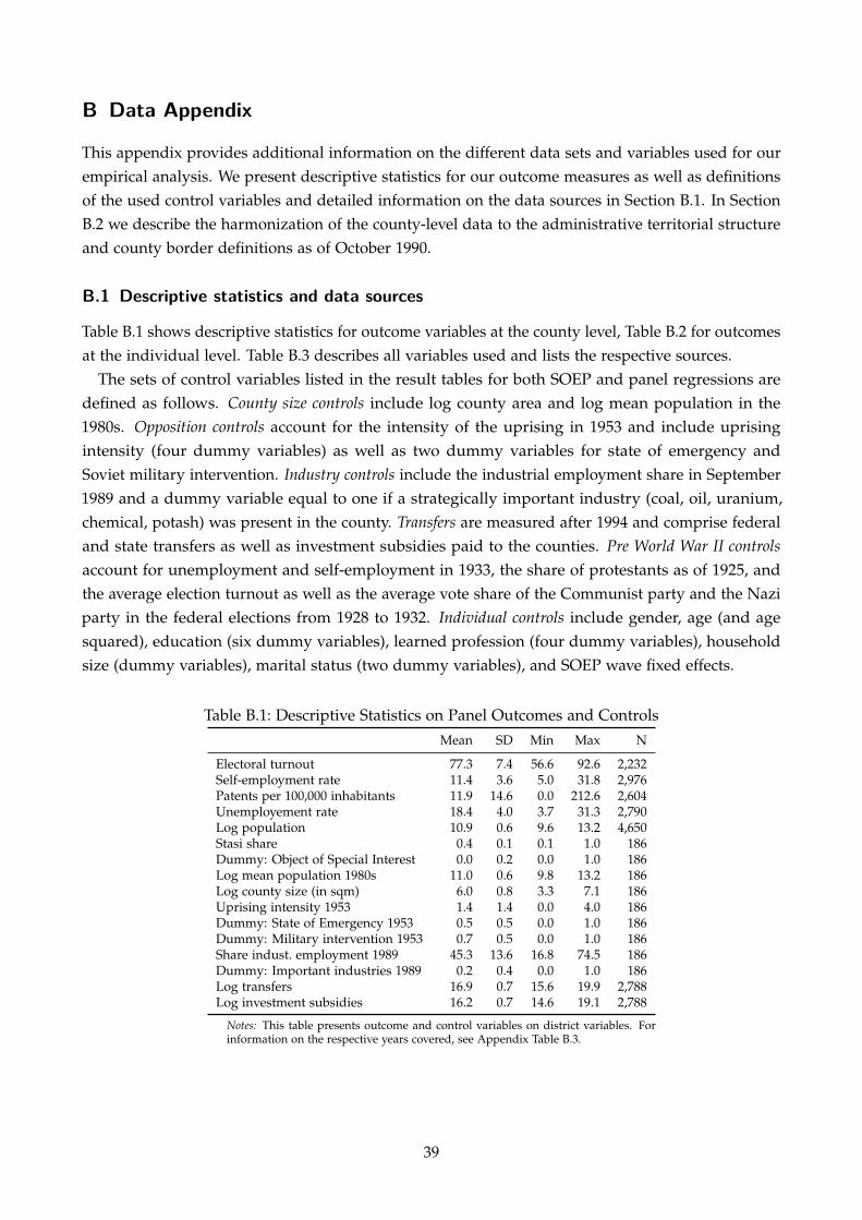
B Data Appendix

This appendix provides additional information on the different data sets and variables used for ourempirical analysis. We present descriptive statistics for our outcome measures as well as definitionsof the used control variables and detailed information on the data sources in Section B.1. In SectionB.2 we describe the harmonization of the county-level data to the administrative territorial structureand county border definitions as of October 1990.

B.1 Descriptive statistics and data sources

Table B.1 shows descriptive statistics for outcome variables at the county level, Table B.2 for outcomesat the individual level. Table B.3 describes all variables used and lists the respective sources.

The sets of control variables listed in the result tables for both SOEP and panel regressions aredefined as follows. County size controls include log county area and log mean population in the1980s. Opposition controls account for the intensity of the uprising in 1953 and include uprisingintensity (four dummy variables) as well as two dummy variables for state of emergency andSoviet military intervention. Industry controls include the industrial employment share in September1989 and a dummy variable equal to one if a strategically important industry (coal, oil, uranium,chemical, potash) was present in the county. Transfers are measured after 1994 and comprise federaland state transfers as well as investment subsidies paid to the counties. Pre World War II controlsaccount for unemployment and self-employment in 1933, the share of protestants as of 1925, andthe average election turnout as well as the average vote share of the Communist party and the Naziparty in the federal elections from 1928 to 1932. Individual controls include gender, age (and agesquared), education (six dummy variables), learned profession (four dummy variables), householdsize (dummy variables), marital status (two dummy variables), and SOEP wave fixed effects.

Table B.1: Descriptive Statistics on Panel Outcomes and ControlsMean SD Min Max N

Electoral turnout 77.3 7.4 56.6 92.6 2,232Self-employment rate 11.4 3.6 5.0 31.8 2,976Patents per 100,000 inhabitants 11.9 14.6 0.0 212.6 2,604Unemployement rate 18.4 4.0 3.7 31.3 2,790Log population 10.9 0.6 9.6 13.2 4,650Stasi share 0.4 0.1 0.1 1.0 186Dummy: Object of Special Interest 0.0 0.2 0.0 1.0 186Log mean population 1980s 11.0 0.6 9.8 13.2 186Log county size (in sqm) 6.0 0.8 3.3 7.1 186Uprising intensity 1953 1.4 1.4 0.0 4.0 186Dummy: State of Emergency 1953 0.5 0.5 0.0 1.0 186Dummy: Military intervention 1953 0.7 0.5 0.0 1.0 186Share indust. employment 1989 45.3 13.6 16.8 74.5 186Dummy: Important industries 1989 0.2 0.4 0.0 1.0 186Log transfers 16.9 0.7 15.6 19.9 2,788Log investment subsidies 16.2 0.7 14.6 19.1 2,788

Notes: This table presents outcome and control variables on district variables. Forinformation on the respective years covered, see Appendix Table B.3.

39

Table B.2: Descriptive Statistics on SOEP OutcomesMean SD Min Max N

Dummy: Trust in strangers 0.14 0.35 0.00 1.00 3,389× Born before 1940 0.18 0.38 0.00 1.00 895× Born 1940–1961 0.14 0.34 0.00 1.00 1,867× Born after 1961 0.11 0.31 0.00 1.00 627× Stayed in county 0.15 0.36 0.00 1.00 2,713× Moved 0.11 0.31 0.00 1.00 676

Negative reciprocity 9.22 4.23 3.00 21.00 3,014× Born before 1940 8.80 4.41 3.00 21.00 754× Born 1940–1961 9.10 4.11 3.00 21.00 1,673× Born after 1961 10.09 4.25 3.00 21.00 587× Stayed in county 9.26 4.20 3.00 21.00 2,443× Moved 9.03 4.40 3.00 21.00 571

Dummy: Attend elections 0.71 0.45 0.00 1.00 3,116× Born before 1940 0.80 0.40 0.00 1.00 789× Born 1940–1961 0.69 0.46 0.00 1.00 1,732× Born after 1961 0.65 0.48 0.00 1.00 595× Stayed in county 0.69 0.46 0.00 1.00 2,484× Moved 0.77 0.42 0.00 1.00 632

Dummy: Engagement in local politics 0.11 0.31 0.00 1.00 3,563× Born before 1940 0.13 0.33 0.00 1.00 926× Born 1940–1961 0.12 0.32 0.00 1.00 1,959× Born after 1961 0.06 0.24 0.00 1.00 678× Stayed in county 0.11 0.32 0.00 1.00 2,890× Moved 0.09 0.29 0.00 1.00 673

Log monthly gross labor income 7.52 0.66 4.09 9.52 1,773× Born before 1940 5.81 0.44 5.03 6.92 15× Born 1940–1961 7.52 0.66 4.09 9.21 1,215× Born after 1961 7.56 0.62 5.01 9.52 543× Stayed in county 7.50 0.65 4.09 9.52 1,358× Moved 7.57 0.72 5.01 9.21 415

Notes: This table presents descriptives statistics on SOEP outcome variables. For infor-mation on the respective years covered, see Appendix Table B.3.

Table B.3: Data sources and variable construction

Variable Years Source

Panel A – Stasi data (see Section 3.1)

Spy density 1980–1988 The main explanatory variable of interest, regional spy density, is calculated asthe average spy density at the county level in the period 1980–1988 (see Section3.1 for details). Data on spies, called unofficial collaborators, are based onofficial Stasi records published by the Agency of the Federal Commissioner forthe Stasi Records (Bundesbeauftragter fur die Unterlagen des Staatssicherheitsdienstesder ehemaligen Deutschen Demokratischen Republik, BStU) and compiled by Muller-Enbergs (2008). Population figures come from the Statistical Yearbooks of theGDR.

continued

40

Table B.3 continued


Our measure of spy density covers unofficial collaborators for political-operativepenetration, homeland defense, or special operations, as well as leading inform-ers (IM zur politisch-operativen Durchdringung und Sicherung des Verantwortungs-bereiches, IM der Abwehr mit Feindverbindung bzw. zur unmittelbaren Bearbeitung imVerdacht der Feindtatigkeit stehender Personen, IM im besonderen Einsatz, Fuhrungs-IM). In cases where Stasi held offices in Objects of Special Interest, the numberof spies attached to these offices was added to the number of spies in therespective county.

Panel B – Individual SOEP data (see Section 3.2)

Attend elections 2005, 2009 The question exploited reads as follows: “If the next election to the German‘Bundestag’ were next Sunday, would you vote?”. Response options weregiven on a five-point scale to allow respondents to express different levels ofconviction (not) to vote (“in no case”, “probably not”, “possibly”, “probably”,“in any case”). We construct a zero/one dummy grouping the former three andthe latter two response options.

Engagement inlocal politics 2001, 2007 Respondents are questioned about their involvement in citizen’s groups, politi-

cal parties and local governments (the question reads: “Which of the followingactivities do you take part in during your free time?”). Response options varyon a four point scale indicating weekly, monthly, less often or no involvement atall. We construct a zero/one dummy variable indicating whether respondentsare involved at all. Note that information on individuals’ engagement in localpolitics is provided in additional waves as well. We choose the years of 2001and 2007 to cover similar points in time with all of our four measures of socialcapital.

Labor income 2003, 2008 Information on current monthly gross labor income is provided in every wavefor East German respondents since 1992. As we aim to identify the directrelationship between surveillance, trust, and economic performance, we focuson those two waves in which both trust and wages can be observed.

Reciprocity 2005, 2010 We use three statements on negative reciprocity, response options varying ona seven-point scale. We follow Dohmen et al. (2009) by combining the threequestions into one single measure. The respective questions read as follows: (i)“If I suffer a serious wrong, I will take revenge as soon as possible, no matterwhat the cost,” (ii) “If somebody puts me in a difficult position, I will do thesame to him/her,” and (iii) “If somebody offends me, I will offend him/herback.”

Trust in strangers 2003, 2008 The question on interpersonal trust reads as follows: “If one is dealing withstrangers, it is better to be careful before one can trust them.” Response optionswere given on a four-point scale, allowing the respondents to totally or slightlyagree, or totally or slightly disagree with the given statements. To simplifyinterpretation of our estimates we group the first and latter two answers.

Control variables The set of control variables includes information on the respondents’ age, sex,household size, marital status, education and learned profession. As differentmeasures of social capital are measured in various waves of the survey; samplesslightly differ for the outcome variables of interest.

continued

41

Table B.3 continued


Panel C – County-level data (see Section 3.3)

Election turnout 1924–1932 We use election turnout in the federal elections in the Weimar Republic in05/1924, 12/1924, 1928, 1930, 07/1932 and 11/1932. The data is provided inthe replication data of King et al. (2008), available at the Harvard Dataverse,handle: hdl/1902.1/11193.

1990–2009 Data on regional election turnout in the federal elections in 1990, 1994, 1998,2002, 2005 and 2009 are provided by the Federal Returning Officer (Bun-deswahlleiter).

Industry controls 1989 Industry composition is measured by means of the share of employees in theindustrial sector as of September 1989, reported in Rudolph (1990). We furthercollect information from various sources whether large enterprises from theuranium, coal, potash, oil or chemical industry were located in the respectivecounty. We construct a zero/one dummy based on this data.

Patents 1928–1929 We approximate county-level patent filings in 1928 and 1929 with data onhigh-value patents provided by Jochen Streb. High-value patents are defined aspatents with a life span of at least ten years (Streb et al., 2006).

1993–2005 Information on post re-unification patent filings come from the German Patentand Trade Mark Office (Deutsches Patent- und Markenamt). Yearly data areprovided for 1995–2005; for 1992–1994 the aggregated number of patents isgiven. We assign the average number of patents to the year of 1993.

Political ideology 1928–1932 We proxy historic political ideology by the mean vote shares of the Communistparty (Kommunistische Partei Deutschlands, KPD) and the Nazi party (National-sozialistische Deutsche Arbeiterpartei, NSDAP) in the federal elections in 1928, 1930,07/1932 and 11/1932 to construct two distinct measures of political ideology.Data on Weimar Republic election results are based on King et al. (2008).

Population 1925–1933 Population figures for the Weimar Republic are obtained from King et al. (2008)and Falter and Hanisch (1990).

1980–1989 Data collected from the Statistical Yearbooks of the German Democratic Repub-lic (Statistische Jahrbucher der Deutschen Demokratischen Republik).

1990–2009 Collected from the Regional Database Germany (Regionaldatenbank Deutschland),the Statistical Offices of the Federal States (Statistische Landesamter) and theWorking Group Regional Accounts (Arbeitskreis Volkswirtschaftliche Gesamtrech-nungen der Lander).

Religion 1925 The share of protestants in the population was published in the 1925 censusof the Weimar Republic (Volkszahlung 1925). Our data stems from King et al.(2008).

Revenues 1995–2009 Data on revenues are obtained from the Regional Database Germany (Region-aldatenbank Deutschland). Revenues cover monetary transfers from the federaland state level (allgemeine Zuweisungen und Umlagen von Bund, Land, Gemein-den/Gemeindeverbanden) as well as investment subsidies granted to the counties(Zuweisungen und Zuschusse fur Investitionsforderungen).

continued

42

Table B.3 continued


Self-employment 1925, 1933 County-level self-employment rates from the 1925 and 1933 censuses of theWeimar Republic (Volks- und Berufszahlung 1925 und 1933). Data for 1925 areobtained from Falter and Hanisch (1990); data for 1933 from King et al. (2008).Note that numbers for 1925 refer to households and should be considered asan approximation of the self-employment rate.

1996–2009 County-level data on the share of self-employed is available in the INKAR database of the Federal Institute for Research on Building, Urban Affairs and SpatialDevelopment (Bundesinstitut fur Bau-, Stadt- und Raumforschung, BBSR).

Unemployment 1933 County-level unemployment rates are based on the 1933 census of the WeimarRepublic (Volks- und Berufszahlung 1933), provided in King et al. (2008).

1996–2009 Monthly county-level unemployment rates are made available from March 1996to December 2009 by the Federal Employment Agency (Bundesagentur fur Arbeit).We calculate yearly means from this data.

Uprising 1953 We use cartographic statistics published by the former West German FederalMinistry of Intra-German Relations (Bundesministerium fur gesamtdeutsche Fragen)to create two dummy variables indicating whether the regime declared a state ofemergency and whether the Soviet military intervened in the particular county.In addition, the data provides an ordinal, additive measure of strike intensity(“none”, “strike”, “demonstration”, “riot”, “liberation of prisoners”). The mapis available in the archives of the Federal Foundation for the Reappraisal of theSED Dictatorship (Bundesstiftung zur Aufarbeitung der SED-Diktatur), signature:EA 111 1889.

B.2 Redrawn county borders and data harmonization

We combine county-level data from various sources and decades in this study. Since 1925, the firstyear in our data set, county borders have been redrawn multiple times. To account for these territorialchanges, we harmonize all county-level data to borders as of October 1990.

The Federal Institute for Research on Building, Urban Affairs and Spatial Development (BBSR)provides population and area weighting factors for all county border reforms from 1991 onwardsto harmonize the data. We rely on population weights because population shares yield the mostaccurate harmonization of different border definitions with regard to our outcomes, which are mainlydriven by people, not space. The outlined procedure is important as the number of East Germancounties was gradually reduced from 216 at the time of the German reunification to 87 in 2009 (theboroughs of East Berlin counting as one single county). Of course, this harmonization is only validwhen looking at county-level aggregates and not individual data. The panel dimension of the SOEP,however, allows us to identify individuals’ county of residence prior to the fall of the Berlin Wall.

Unfortunately, there are no administrative weighting factors available for the harmonization ofcounty borders prior to reunification. However, there were only minor territorial reforms between1953 and 1990, the period we cover with our GDR data. In ten cases, neighboring counties weremerged together. In five cases, bigger cities became independent from the surrounding county(Stadtkreise). We manually account for these administrative changes using detailed maps and otherhistorical sources. When merging two counties, we always use the maximum for each of the three

43

riot variables (state of emergency, Soviet military intervention, strike intensity). In case new countieswere constituted, we assign historical values of the emitting county to the created one.

When harmonizing data from the Weimar Republic with county borders as of 1990, considerableadministrative territorial reforms have to be taken into account. Due to the lack of adequatepopulation weighting factors, the harmonization is based on geospatial area weighting factors(Goodchild and Lam, 1980). We merge the corresponding shapefiles from the Weimar Republic withthe shapefile for 1990 to determine weighting factors that allow to adjust the historical data to thecounty borders as of 1990. Given that most of our outcomes and control variables refer to people andnot space, it needs to be stressed that this procedure is afflicted with some degree of imprecision.Given the long time span, the numerous territorial reforms, and the lack of population weightingfactors, this procedure is, however, the most accurate harmonization procedure we can apply.

44

The Economic Costs of Mass Surveillance: Insights from ...ftp.iza.org/dp9245.pdf · The Economic...

Documents

Transcript of The Economic Costs of Mass Surveillance: Insights from ...ftp.iza.org/dp9245.pdf · The Economic...