
The Cost of Privatization Hagit Attiya Eshcar Hillel Technion & EPFLTechnion.
1
1
Computational PhotographyComputational PhotographyComputer Science 203.4790Semester B 2009-2010Lecture: Sunday 12:00-15:00 Room: 303
Dr. Hagit [email protected]: 415Office Hours: by appointment
Course Internet Site: http://cs.haifa.ac.il/courses/compPhoto
2
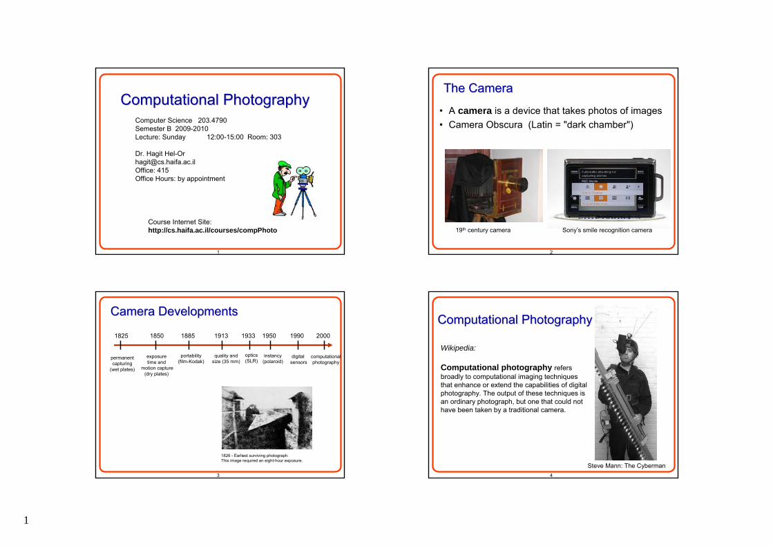
The CameraThe Camera
• A camera is a device that takes photos of images • Camera Obscura (Latin = "dark chamber")
19th century camera Sony’s smile recognition camera
3
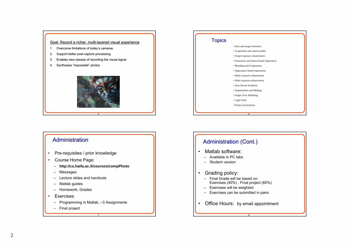
Camera DevelopmentsCamera Developments
1825 19901913
permanent capturing
(wet plates)
1850
exposuretime and
motion capture(dry plates)
digital sensors
quality and size (35 mm)
1885
portability(film-Kodak)
1933
optics (SLR)
1950
instancy(polaroid)
2000
computationalphotography
1826 - Earliest surviving photograph. This image required an eight-hour exposure.
4
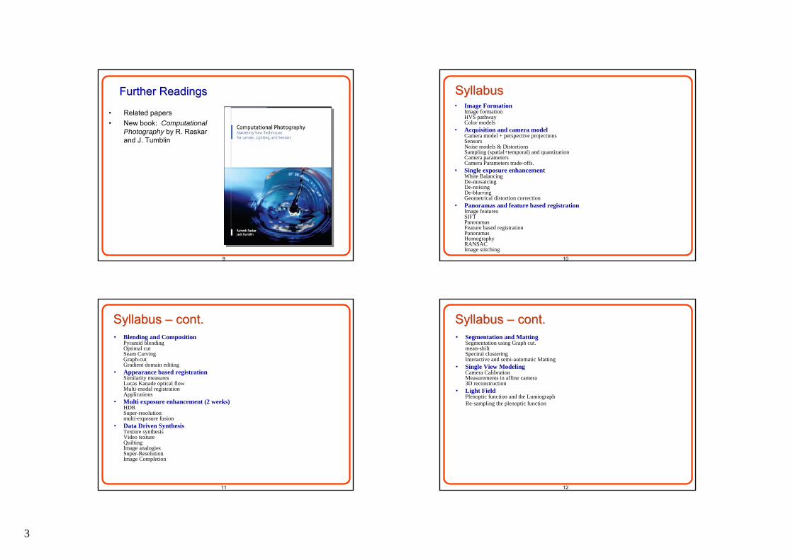
Computational PhotographyComputational Photography
Wikipedia:
Computational photography refers broadly to computational imaging techniques that enhance or extend the capabilities of digital photography. The output of these techniques is an ordinary photograph, but one that could not have been taken by a traditional camera.
Steve Mann: The Cyberman
2
5
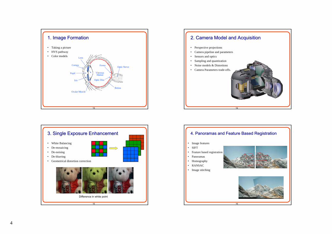
Goal: Record a richer, multiGoal: Record a richer, multi--layered visual experiencelayered visual experience1.1. Overcome limitations of todayOvercome limitations of today’’s camerass cameras
2.2. Support better postSupport better post--capture processingcapture processing
3.3. Enables new classes of recording the visual signal Enables new classes of recording the visual signal
4.4. Synthesize Synthesize ““impossibleimpossible”” photosphotos
6
TopicsTopics
• Project presentation
• Light Field
• Single View Modeling
• Segmentation and Matting
• Data Driven Synthesis
• Multi exposure enhancement
• Multi exposure enhancement
• Appearance-based registration
• Blending and Composition
• Panoramas and feature-based registration
• Single exposure enhancement
• Acquisition and camera model
• Intro and image formation
7
AdministrationAdministration
• Pre-requisites / prior knowledge• Course Home Page:
– http://cs.haifa.ac.il/courses/compPhoto– Messages – Lecture slides and handouts – Matlab guides– Homework, Grades
• Exercises: – Programming in Matlab, ~3 Assignments– Final project
8
Administration (Cont.)Administration (Cont.)
• Matlab software:– Available in PC labs– Student version
• Grading policy: – Final Grade will be based on:
Exercises (40%) , Final project (60%)– Exercises will be weighted – Exercises can be submitted in pairs
• Office Hours: by email appointment
3
9
Further ReadingsFurther Readings
• Related papers• New book: Computational
Photography by R. Raskarand J. Tumblin
10
SyllabusSyllabus• Image Formation
Image formation HVS pathwayColor models
• Acquisition and camera modelCamera model + perspective projectionsSensorsNoise models & DistortionsSampling (spatial+temporal) and quantizationCamera parametersCamera Parameters trade-offs.
• Single exposure enhancementWhite BalancingDe-mosaicingDe-noisingDe-blurringGeometrical distortion correction
• Panoramas and feature based registrationImage featuresSIFTPanoramasFeature based registrationPanoramasHomographyRANSAC Image stitching
11
Syllabus Syllabus –– cont.cont.• Blending and Composition
Pyramid blendingOptimal cutSeam CarvingGraph-cutGradient domain editing
• Appearance based registrationSimilarity measures Lucas Kanade optical flowMulti-modal registrationApplications
• Multi exposure enhancement (2 weeks)HDRSuper-resolutionmulti-exposure fusion
• Data Driven SynthesisTexture synthesisVideo textureQuiltingImage analogiesSuper-ResolutionImage Completion
12
Syllabus Syllabus –– cont.cont.• Segmentation and Matting
Segmentation using Graph cut.mean-shiftSpectral clusteringInteractive and semi-automatic Matting
• Single View ModelingCamera CalibrationMeasurements in affine camera3D reconstruction
• Light FieldPlenoptic function and the LumiographRe-sampling the plenoptic function
4
13
1. Image Formation1. Image Formation
• Taking a picture• HVS pathway• Color models
Optic NerveFovea
Vitreous
Optic Disc
Lens
Pupil
Cornea
Ocular MuscleRetina
Humor
Iris
14
2. Camera Model and Acquisition2. Camera Model and Acquisition
• Perspective projections• Camera pipeline and parameters• Sensors and optics• Sampling and quantization• Noise models & Distortions • Camera Parameters trade-offs.
15
3. Single Exposure Enhancement3. Single Exposure Enhancement
• White Balancing• De-mosaicing• De-noising• De-blurring• Geometrical distortion correction
Difference in white point
16
4. Panoramas and Feature Based Registration4. Panoramas and Feature Based Registration
• Image features• SIFT• Feature based registration• Panoramas• Homography• RANSAC • Image stitching
5
17
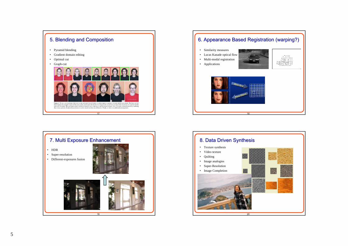
5. Blending and Composition5. Blending and Composition
• Pyramid blending• Gradient domain editing• Optimal cut• Graph-cut
18
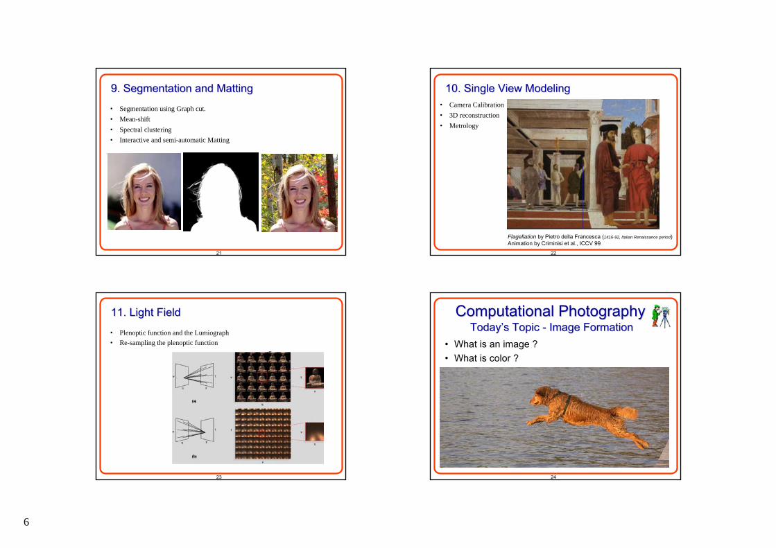
6. Appearance Based Registration (warping?)6. Appearance Based Registration (warping?)
• Similarity measures • Lucas Kanade optical flow• Multi-modal registration• Applications
19
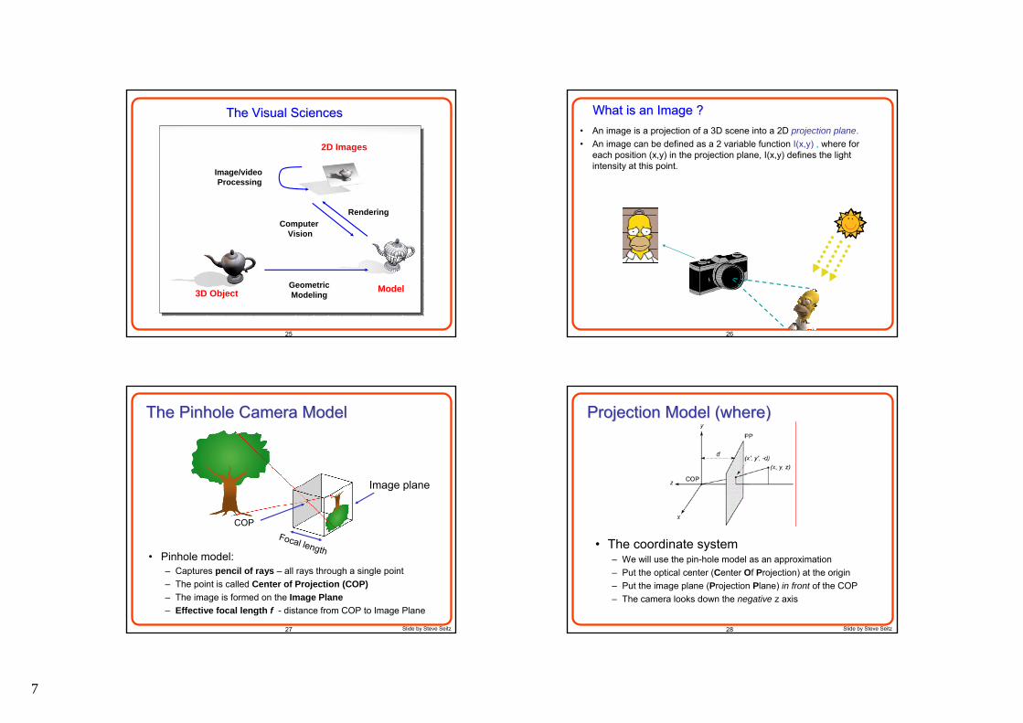
7. Multi Exposure Enhancement 7. Multi Exposure Enhancement
• HDR• Super-resolution• Different-exposures fusion
20
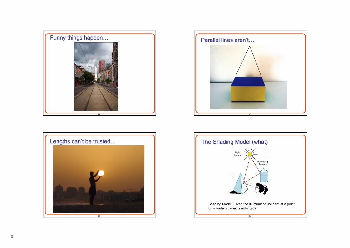
8. Data Driven Synthesis 8. Data Driven Synthesis • Texture synthesis• Video texture• Quilting• Image analogies• Super-Resolution• Image Completion
6
21
9. Segmentation and Matting 9. Segmentation and Matting
• Segmentation using Graph cut.• Mean-shift• Spectral clustering• Interactive and semi-automatic Matting
22
10. Single View Modeling10. Single View Modeling• Camera Calibration• 3D reconstruction• Metrology
Flagellation by Pietro della Francesca (1416-92, Italian Renaissance period)Animation by Criminisi et al., ICCV 99
23
11. Light Field11. Light Field
• Plenoptic function and the Lumiograph• Re-sampling the plenoptic function
24
Computational PhotographyComputational PhotographyTodayToday’’s Topic s Topic -- Image FormationImage Formation
• What is an image ?• What is color ?
7
25
Computer Vision
Rendering
Image/video Processing
Model3D ObjectGeometric Modeling
2D Images
The Visual SciencesThe Visual Sciences
26
What is an Image ?What is an Image ?• An image is a projection of a 3D scene into a 2D projection plane.• An image can be defined as a 2 variable function I(x,y) , where for
each position (x,y) in the projection plane, I(x,y) defines the light intensity at this point.
27
The Pinhole Camera ModelThe Pinhole Camera Model
• Pinhole model:– Captures pencil of rays – all rays through a single point– The point is called Center of Projection (COP)– The image is formed on the Image Plane– Effective focal length f - distance from COP to Image Plane
Slide by Steve Seitz
COP
Image plane
Focal length
28
Projection Model (where)Projection Model (where)
• The coordinate system– We will use the pin-hole model as an approximation– Put the optical center (Center Of Projection) at the origin– Put the image plane (Projection Plane) in front of the COP– The camera looks down the negative z axis
Slide by Steve Seitz
8
29
Funny things happenFunny things happen……
30
Parallel lines arenParallel lines aren’’tt……
31
Lengths canLengths can’’t be trusted...t be trusted...
32
The Shading Model (what)The Shading Model (what)
Shading Model: Given the illumination incident at a point on a surface, what is reflected?
9
33
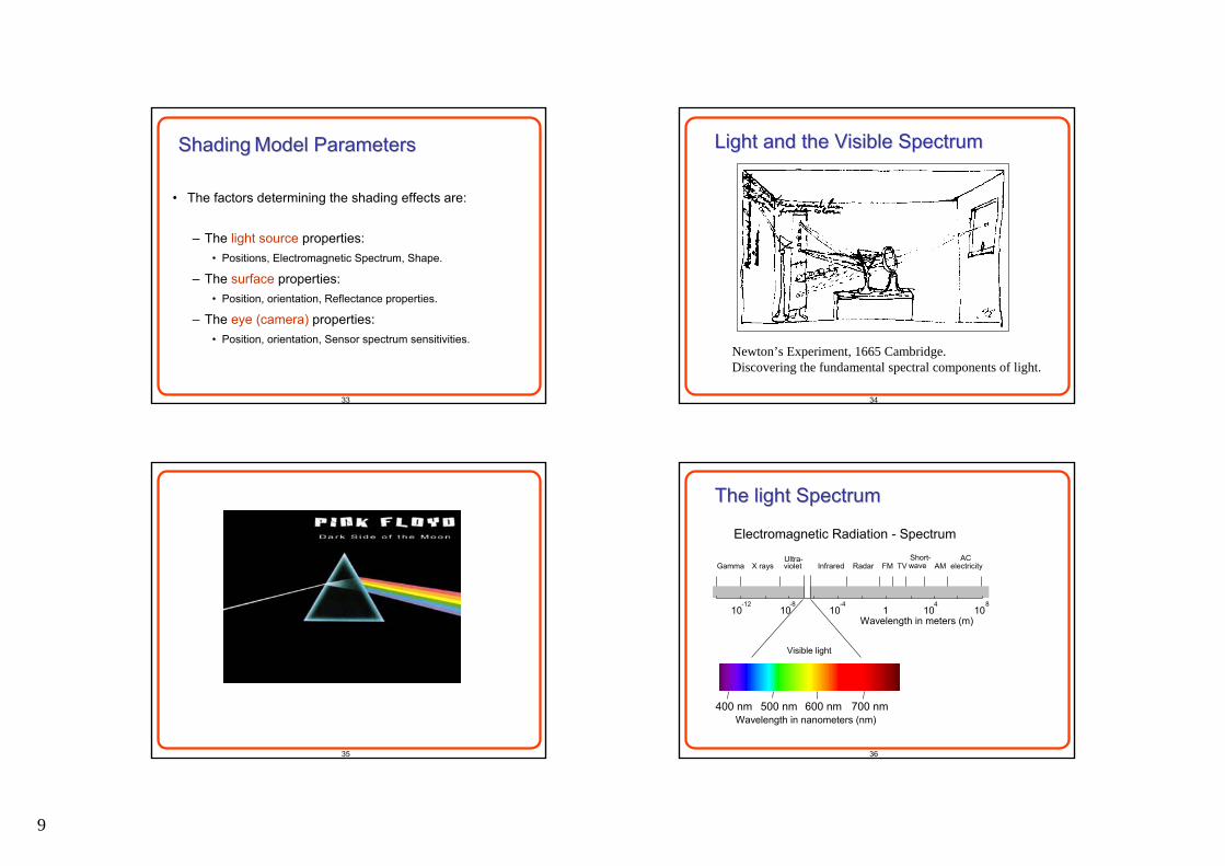
ShadingShading Model ParametersModel Parameters
• The factors determining the shading effects are:
– The light source properties:• Positions, Electromagnetic Spectrum, Shape.
– The surface properties:• Position, orientation, Reflectance properties.
– The eye (camera) properties:• Position, orientation, Sensor spectrum sensitivities.
34
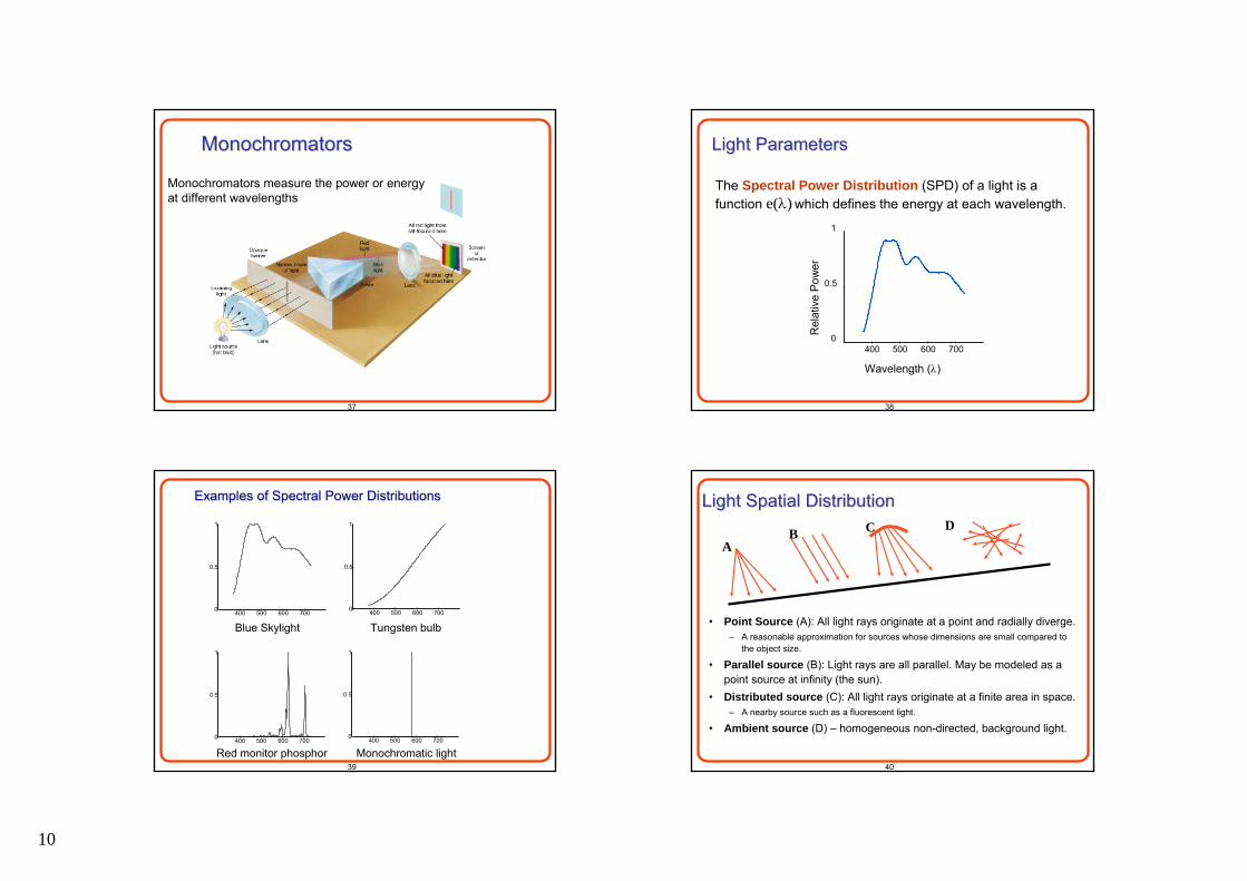
Newton’s Experiment, 1665 Cambridge.Discovering the fundamental spectral components of light.
Light and the Visible SpectrumLight and the Visible Spectrum
35 36
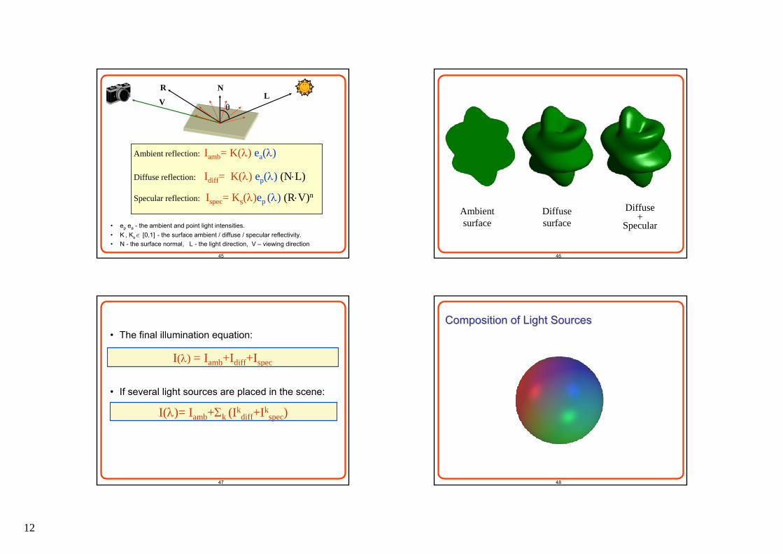
The light SpectrumThe light Spectrum
Electromagnetic Radiation - Spectrum
Gamma X rays Infrared Radar FM TV AMUltra-violet
10-12
10-8
10-4
104
1 108
electricityACShort-
wave
400 nm 500 nm 600 nm 700 nmWavelength in nanometers (nm)
Wavelength in meters (m)
Visible light
10
37
MonochromatorsMonochromators
Monochromators measure the power or energy at different wavelengths
38
The Spectral Power Distribution (SPD) of a light is a function e(λ) which defines the energy at each wavelength.
Wavelength (λ)
400 500 600 7000
0.5
1
Rel
ativ
e P
ower
Light ParametersLight Parameters
39
ExamplesExamples of Spectral Power Distributionsof Spectral Power Distributions
Blue Skylight Tungsten bulb
Red monitor phosphor Monochromatic light
400 500 600 7000
0.5
1
400 500 600 7000
0.5
1
400 500 600 7000
0.5
1
400 500 600 7000
0.5
1
40
Light Spatial DistributionLight Spatial Distribution
• Point Source (A): All light rays originate at a point and radially diverge.– A reasonable approximation for sources whose dimensions are small compared to
the object size.
• Parallel source (B): Light rays are all parallel. May be modeled as a point source at infinity (the sun).
• Distributed source (C): All light rays originate at a finite area in space.– A nearby source such as a fluorescent light.
• Ambient source (D) – homogeneous non-directed, background light.
AB C D
11
41
Specular reflectionmirror like reflection at the surface
Diffuse (lambertian) reflection reflected randomly between color particlesreflection is equal in all directions
Incident light Specular reflection
Diffuse reflection
normal
Surface ParametersSurface Parameters
42
Different Types of Surfaces
43
400 500 600 700
0.2
0.40.6
0.81
400 500 600 700
0.2
0.40.6
0.81
400 500 600 700
0.20.4
0.60.8
1
400 500 600 700
0.20.4
0.60.8
1
Surface Body Reflectances (albedo)
Yellow Red
Blue Gray
Wavelength (nm)
Spectral Property of Diffuse SurfacesSpectral Property of Diffuse Surfaces
44
θ
NL
R
V
Ambient reflection: Iamb= K(λ) ea(λ)
Diffuse reflection: Idiff= K(λ) ep(λ) (N⋅L)
Specular reflection: Ispec= Ks(λ)ep (λ) (R⋅V)n
• ea ep - the ambient and point light intensities. • K , Ks ∈ [0,1] - the surface ambient / diffuse / specular reflectivity. • N - the surface normal, L - the light direction, V – viewing direction
Surface propertiesLight properties
geometry
12
45
θ
NL
R
V
Ambient reflection: Iamb= K(λ) ea(λ)
Diffuse reflection: Idiff= K(λ) ep(λ) (N⋅L)
Specular reflection: Ispec= Ks(λ)ep (λ) (R⋅V)n
• ep ea - the ambient and point light intensities. • K , Ks ∈ [0,1] - the surface ambient / diffuse / specular reflectivity. • N - the surface normal, L - the light direction, V – viewing direction
46
Diffusesurface
Ambientsurface
Diffuse +
Specular
47
I(λ) = Iamb+Idiff+Ispec
• The final illumination equation:
• If several light sources are placed in the scene:
I(λ)= Iamb+Σk (Ikdiff+Ik
spec)
48
Composition of Light SourcesComposition of Light Sources
13
49
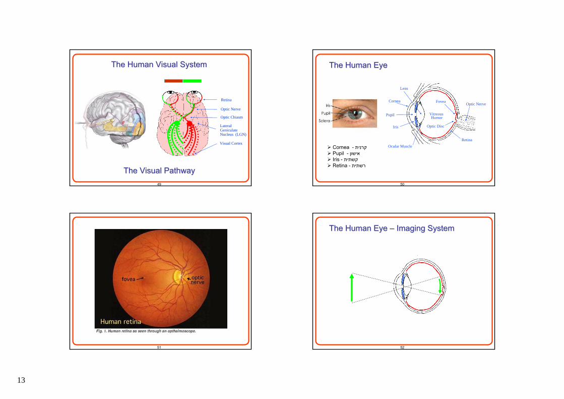
The Visual PathwayThe Visual Pathway
Retina
Optic Nerve
Optic Chiasm
LateralGeniculateNucleus (LGN)
Visual Cortex
The Human Visual SystemThe Human Visual System
50
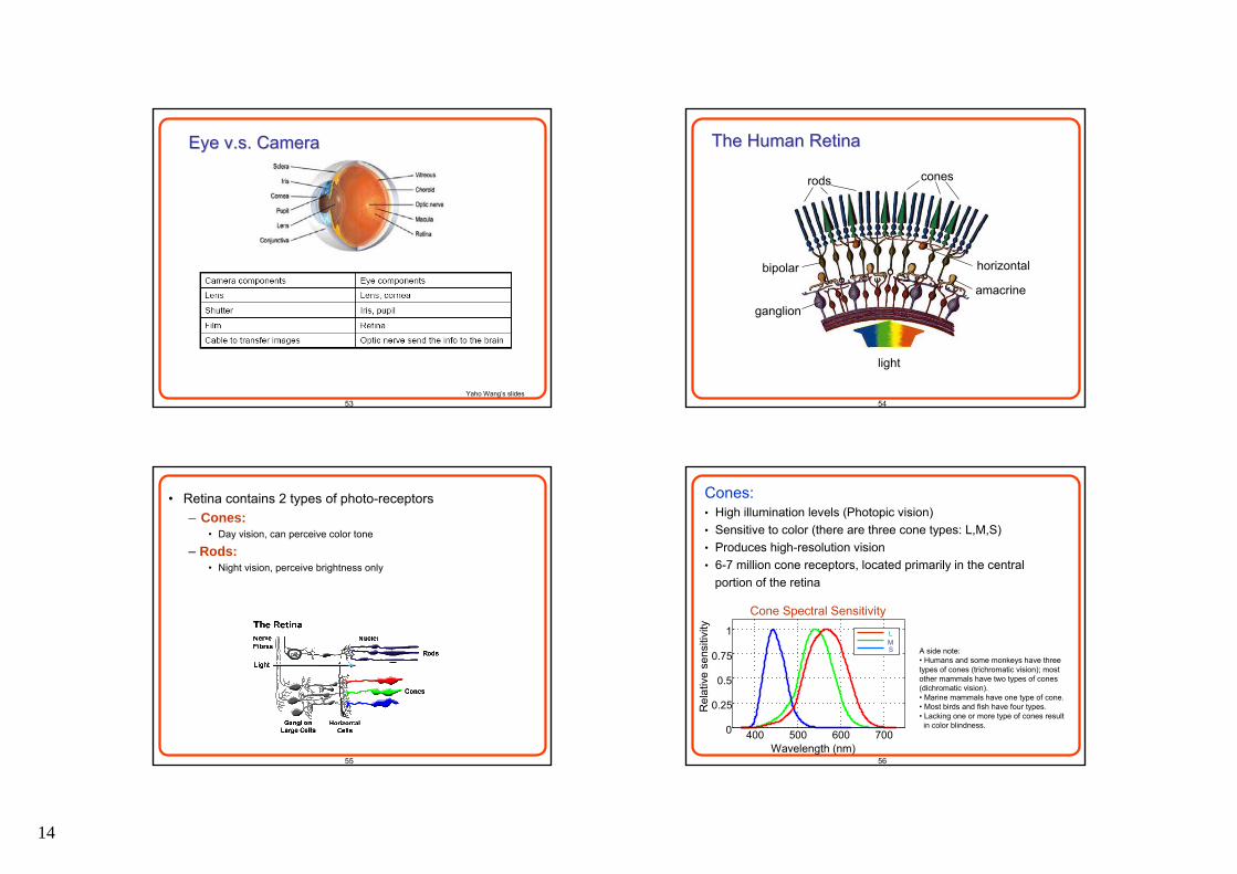
Optic NerveFovea
Vitreous
Optic Disc
Lens
Pupil
Cornea
Ocular MuscleRetina
Humor
Iris
The Human EyeThe Human Eye
Cornea - קרנית Pupil - אישו ן Iris - קשתית Retina - רשתית
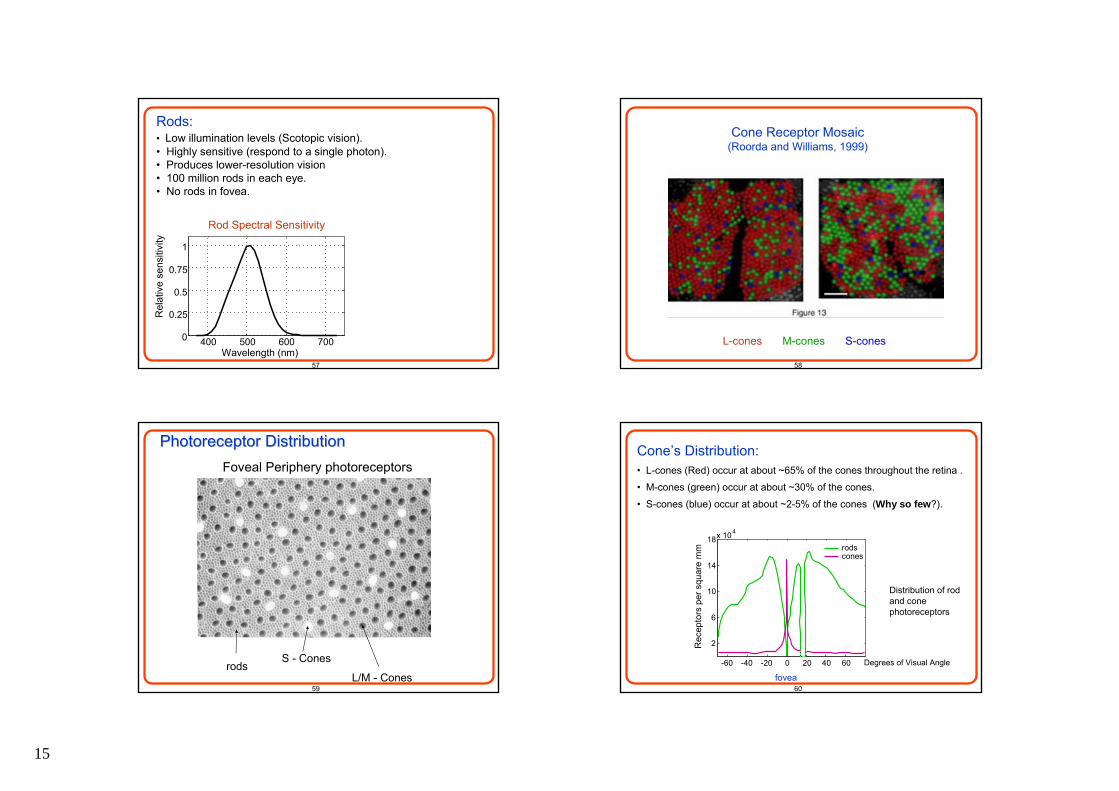
51 52
The Human Eye The Human Eye –– Imaging SystemImaging System
14
53
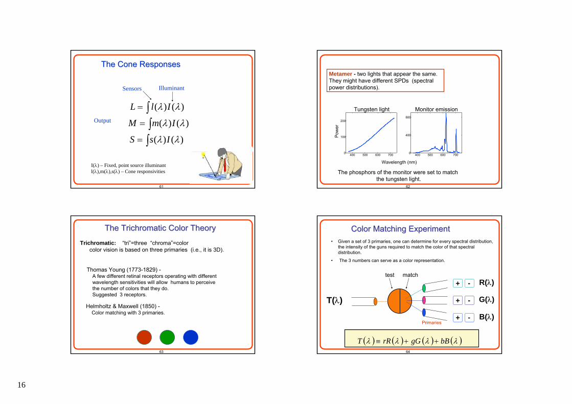
Eye Eye v.sv.s. Camera. Camera
Yaho Wang’s slides54
light
rods cones
horizontal
amacrine
bipolar
ganglion
The Human RetinaThe Human Retina
55
• Retina contains 2 types of photo-receptors– Cones:
• Day vision, can perceive color tone
– Rods: • Night vision, perceive brightness only
56
Cones:• High illumination levels (Photopic vision)• Sensitive to color (there are three cone types: L,M,S)• Produces high-resolution vision• 6-7 million cone receptors, located primarily in the central
portion of the retina
Wavelength (nm)
Rel
ativ
e se
nsiti
vity
Cone Spectral Sensitivity
400 500 600 7000
0.25
0.5
0.75
1ML
SM
A side note:• Humans and some monkeys have three types of cones (trichromatic vision); most other mammals have two types of cones (dichromatic vision).• Marine mammals have one type of cone.• Most birds and fish have four types. • Lacking one or more type of cones result in color blindness.
15
57
Rods:• Low illumination levels (Scotopic vision).• Highly sensitive (respond to a single photon).• Produces lower-resolution vision• 100 million rods in each eye.• No rods in fovea.
Wavelength (nm)
Rel
ativ
e se
nsiti
vity
400 500 600 7000
0.25
0.5
0.75
1
Rod Spectral Sensitivity
58
Cone Receptor Mosaic(Roorda and Williams, 1999)
L-cones M-cones S-cones
59
rodsS - Cones
L/M - Cones
Foveal Periphery photoreceptors
Photoreceptor Distribution Photoreceptor Distribution
60
Distribution of rod and cone photoreceptors
Degrees of Visual Angle
Rec
epto
rs p
er s
quar
e m
m
-60 -40 -20 0 20 40 60
2
6
10
14
18x 104
rodscones
Cone’s Distribution:• L-cones (Red) occur at about ~65% of the cones throughout the retina .
• M-cones (green) occur at about ~30% of the cones.
• S-cones (blue) occur at about ~2-5% of the cones (Why so few?).
fovea
16
61
The Cone ResponsesThe Cone Responses
IlluminantSensors
I(λ) – Fixed, point source illuminantl(λ),m(λ),s(λ) – Cone responsivities
Output∫= )()( λλ IlL
∫= )()( λλ ImM
∫= )()( λλ IsS
62
Metamer - two lights that appear the same. They might have different SPDs (spectral power distributions).
400 500 600 7000
400
800
400 500 600 7000
100
200
Wavelength (nm)
Pow
er
The phosphors of the monitor were set to match the tungsten light.
Tungsten light Monitor emission
63
The The TrichromaticTrichromatic Color TheoryColor Theory
Thomas Young (1773-1829) -A few different retinal receptors operating with different wavelength sensitivities will allow humans to perceivethe number of colors that they do.Suggested 3 receptors.
Helmholtz & Maxwell (1850) -Color matching with 3 primaries.
Trichromatic: “tri”=three “chroma”=colorcolor vision is based on three primaries (i.e., it is 3D).
64
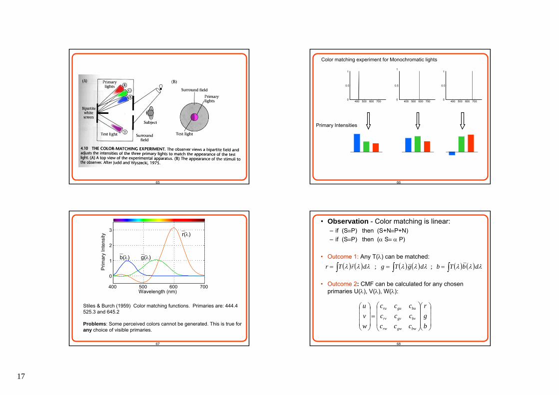
Color Matching ExperimentColor Matching Experiment
+ -
+ -
+ -
test match
Primaries
• Given a set of 3 primaries, one can determine for every spectral distribution, the intensity of the guns required to match the color of that spectral distribution.
• The 3 numbers can serve as a color representation.
( ) ( ) ( ) ( )λλλλ bBgGrRT ++≡
R(λ)
G(λ)
B(λ)
T(λ)
17
65 66
Color matching experiment for Monochromatic lights
400 500 600 7000
0.5
1
400 500 600 7000
0.5
1
400 500 600 7000
0.5
1
Primary Intensities
67
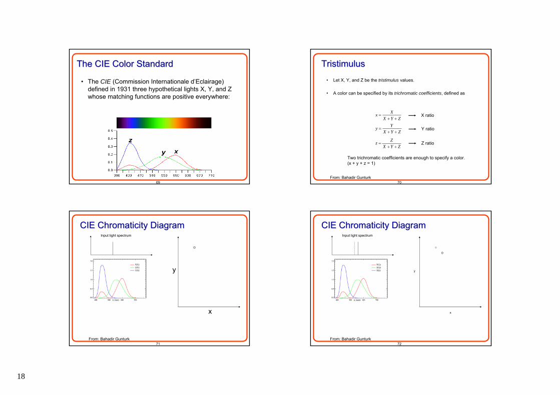
r(λ)
g(λ)b(λ)
400 500 600 700
0
1
2
3
Wavelength (nm)
Prim
ary
Inte
nsity
Stiles & Burch (1959) Color matching functions. Primaries are: 444.4 525.3 and 645.2
Problems: Some perceived colors cannot be generated. This is true for any choice of visible primaries.
68
• Observation - Color matching is linear:– if (S≡P) then (S+N≡P+N) – if (S≡P) then (α S≡ α P)
• Outcome 1: Any T(λ) can be matched:
• Outcome 2: CMF can be calculated for any chosen primaries U(λ), V(λ), W(λ):
( ) ( ) ( ) ( ) ( ) ( ) λλλλλλλλλ dbTbdgTgdrTr ∫∫∫ === ;;
⎟⎟⎟
⎠
⎞
⎜⎜⎜
⎝
⎛
⎟⎟⎟
⎠
⎞
⎜⎜⎜
⎝
⎛
=⎟⎟⎟
⎠
⎞
⎜⎜⎜
⎝
⎛
bgr
ccccccccc
wvu
bwgwrw
bvgvrv
buguru
18
69
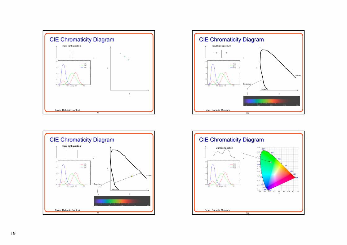
• The CIE (Commission Internationale d’Eclairage) defined in 1931 three hypothetical lights X, Y, and Z whose matching functions are positive everywhere:
The CIE Color StandardThe CIE Color Standard
70
TristimulusTristimulus• Let X, Y, and Z be the tristimulus values.
• A color can be specified by its trichromatic coefficients, defined as
XxX Y Z
=+ +
YyX Y Z
=+ +
ZzX Y Z
=+ +
X ratio
Y ratio
Z ratio
Two trichromatic coefficients are enough to specify a color. (x + y + z = 1)
From: Bahadir Gunturk
71
CIE Chromaticity DiagramCIE Chromaticity DiagramInput light spectrum
x
y
From: Bahadir Gunturk72
CIE Chromaticity DiagramCIE Chromaticity DiagramInput light spectrum
x
y
From: Bahadir Gunturk
19
73
CIE Chromaticity DiagramCIE Chromaticity DiagramInput light spectrum
x
y
From: Bahadir Gunturk74
CIE Chromaticity DiagramCIE Chromaticity DiagramInput light spectrum
Boundary
x
y
380nm
700nm
From: Bahadir Gunturk
75
CIE Chromaticity DiagramCIE Chromaticity DiagramInput light spectrum
Boundary
x
y
380nm
700nm
From: Bahadir Gunturk
Input light spectrum
76
CIE Chromaticity DiagramCIE Chromaticity DiagramLight composition
From: Bahadir Gunturk
20
77
CIE Chromaticity DiagramCIE Chromaticity DiagramLight composition
Light composition
From: Bahadir Gunturk78
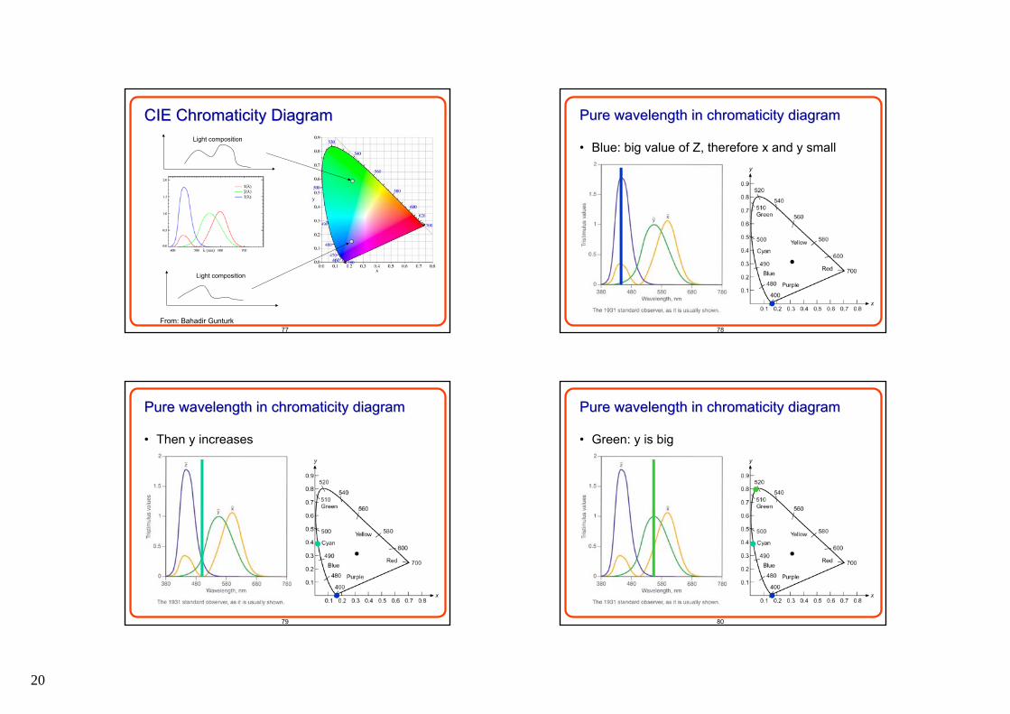
Pure wavelength in chromaticity diagramPure wavelength in chromaticity diagram
• Blue: big value of Z, therefore x and y small
79
Pure wavelength in chromaticity diagramPure wavelength in chromaticity diagram
• Then y increases
80
Pure wavelength in chromaticity diagramPure wavelength in chromaticity diagram
• Green: y is big
21
81
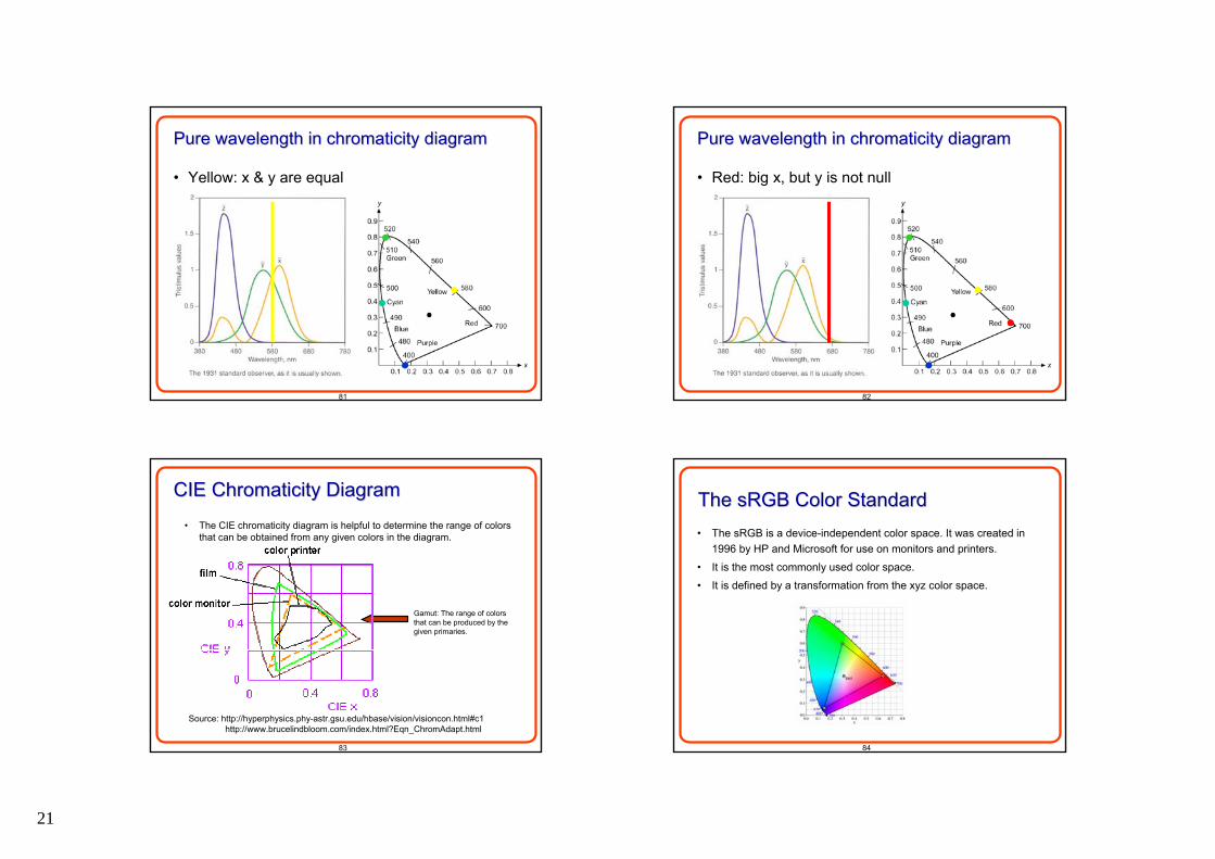
Pure wavelength in chromaticity diagramPure wavelength in chromaticity diagram
• Yellow: x & y are equal
82
Pure wavelength in chromaticity diagramPure wavelength in chromaticity diagram
• Red: big x, but y is not null
83
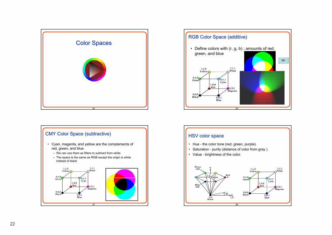
CIE Chromaticity DiagramCIE Chromaticity Diagram• The CIE chromaticity diagram is helpful to determine the range of colors
that can be obtained from any given colors in the diagram.
Source: http://hyperphysics.phy-astr.gsu.edu/hbase/vision/visioncon.html#c1
Gamut: The range of colors that can be produced by the given primaries.
http://www.brucelindbloom.com/index.html?Eqn_ChromAdapt.html
84
• The sRGB is a device-independent color space. It was created in 1996 by HP and Microsoft for use on monitors and printers.
• It is the most commonly used color space.
• It is defined by a transformation from the xyz color space.
The The sRGBsRGB Color StandardColor Standard
22
85
Color SpacesColor Spaces
86
RGB Color Space (additive)RGB Color Space (additive)
• Define colors with (r, g, b) ; amounts of red, green, and blue
87
CMY Color Space (subtractive)CMY Color Space (subtractive)
• Cyan, magenta, and yellow are the complements of red, green, and blue– We can use them as filters to subtract from white– The space is the same as RGB except the origin is white
instead of black
88
HSV color spaceHSV color space
• Hue - the color tone (red, green, purple).• Saturation - purity (distance of color from gray ).• Value - brightness of the color.
23
89
HSV HSV -- a more intuitive color spacea more intuitive color space
Value
Saturation
Hue
90
Opponent ColorsOpponent Colors
Blue-Yellow
LMS
L+M-S
++- +- +++
L-M L+M+S
Red-Green Black-White
Opponent process - possible neural connections:
-
B-Y+
Y-B+
R-G+
G-R+
R-
G+ B-
Y+
Ganglion cells / LGN cells Cortical cells
Color Contrast detectors Color edge detectors
91
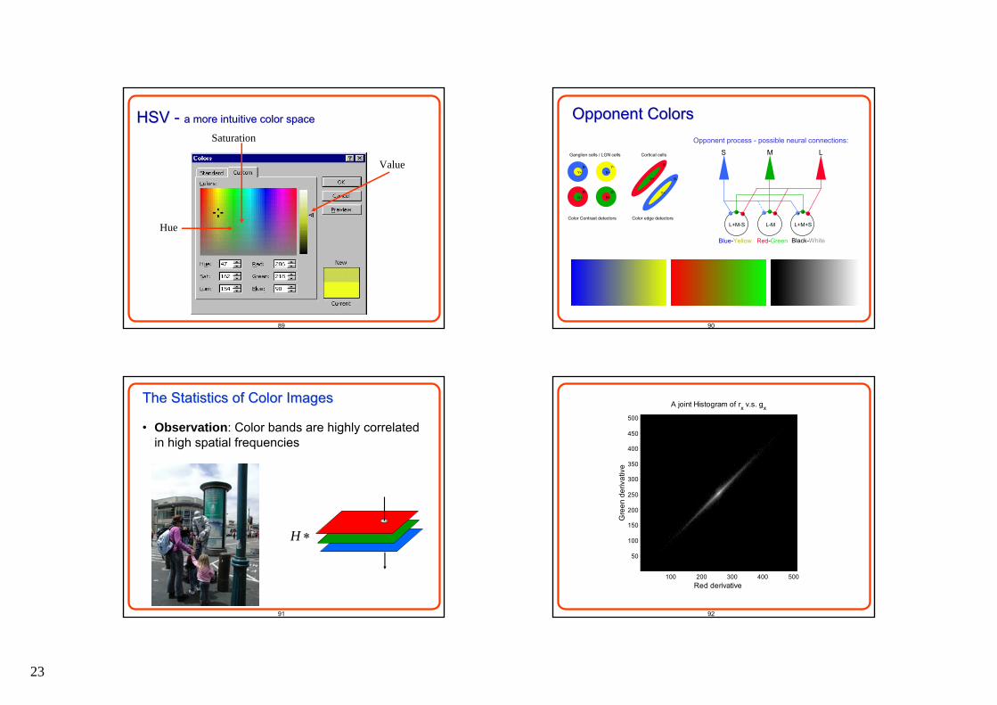
The Statistics of Color ImagesThe Statistics of Color Images
• Observation: Color bands are highly correlated in high spatial frequencies
∗H
92
A joint Histogram of rx v.s. gx
Red derivative
Gre
en d
eriv
ativ
e
100 200 300 400 500
50
100
150
200
250
300
350
400
450
500
24
93
A joint Histogram of gx v.s. bx
Green derivative
Blu
e de
rivat
ive
100 200 300 400 500
50
100
150
200
250
300
350
400
450
500
94
A joint Histogram of rx v.s. bx
Red derivative
Blu
e de
rivat
ive
100 200 300 400 500
50
100
150
200
250
300
350
400
450
500
95 96
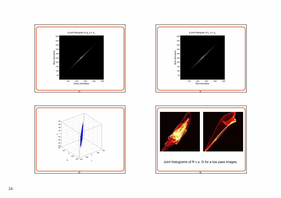
Joint histograms of R v.s. G for a low pass images.
25
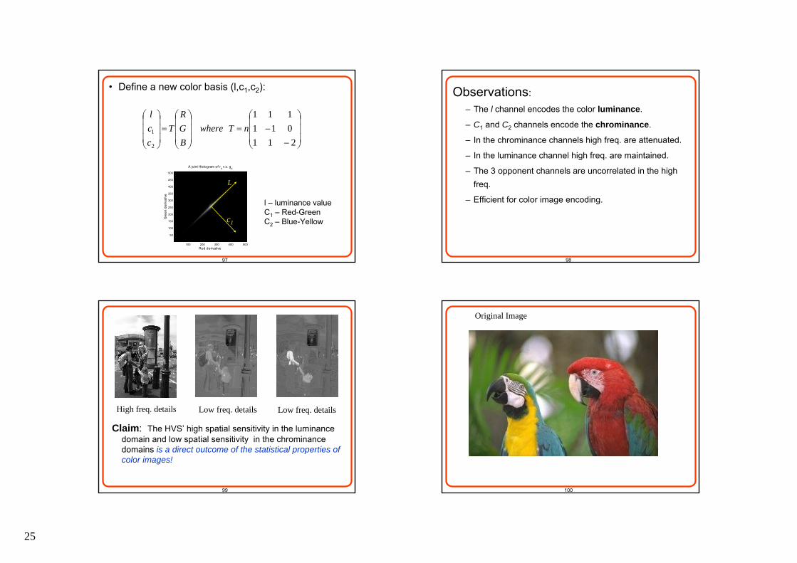
97
• Define a new color basis (l,c1,c2):
⎟⎟⎟
⎠
⎞
⎜⎜⎜
⎝
⎛
−−=
⎟⎟⎟
⎠
⎞
⎜⎜⎜
⎝
⎛=
⎟⎟⎟
⎠
⎞
⎜⎜⎜
⎝
⎛
211011111
2
1 nTwhereBGR
Tccl
l – luminanceC1- red/greenC2 – blue/yellowA joint Histogram of rx v.s. gx
Red derivative
Gre
en d
eriv
ativ
e
100 200 300 400 500
50
100
150
200
250
300
350
400
450
500
L
c1
l – luminance valueC1 – Red-GreenC2 – Blue-Yellow
98
Observations:– The l channel encodes the color luminance.
– C1 and C2 channels encode the chrominance.
– In the chrominance channels high freq. are attenuated.
– In the luminance channel high freq. are maintained.
– The 3 opponent channels are uncorrelated in the high freq.
– Efficient for color image encoding.
99
High freq. details Low freq. details Low freq. details
Claim: The HVS’ high spatial sensitivity in the luminance domain and low spatial sensitivity in the chrominance domains is a direct outcome of the statistical properties of color images!
100
Original Image
26
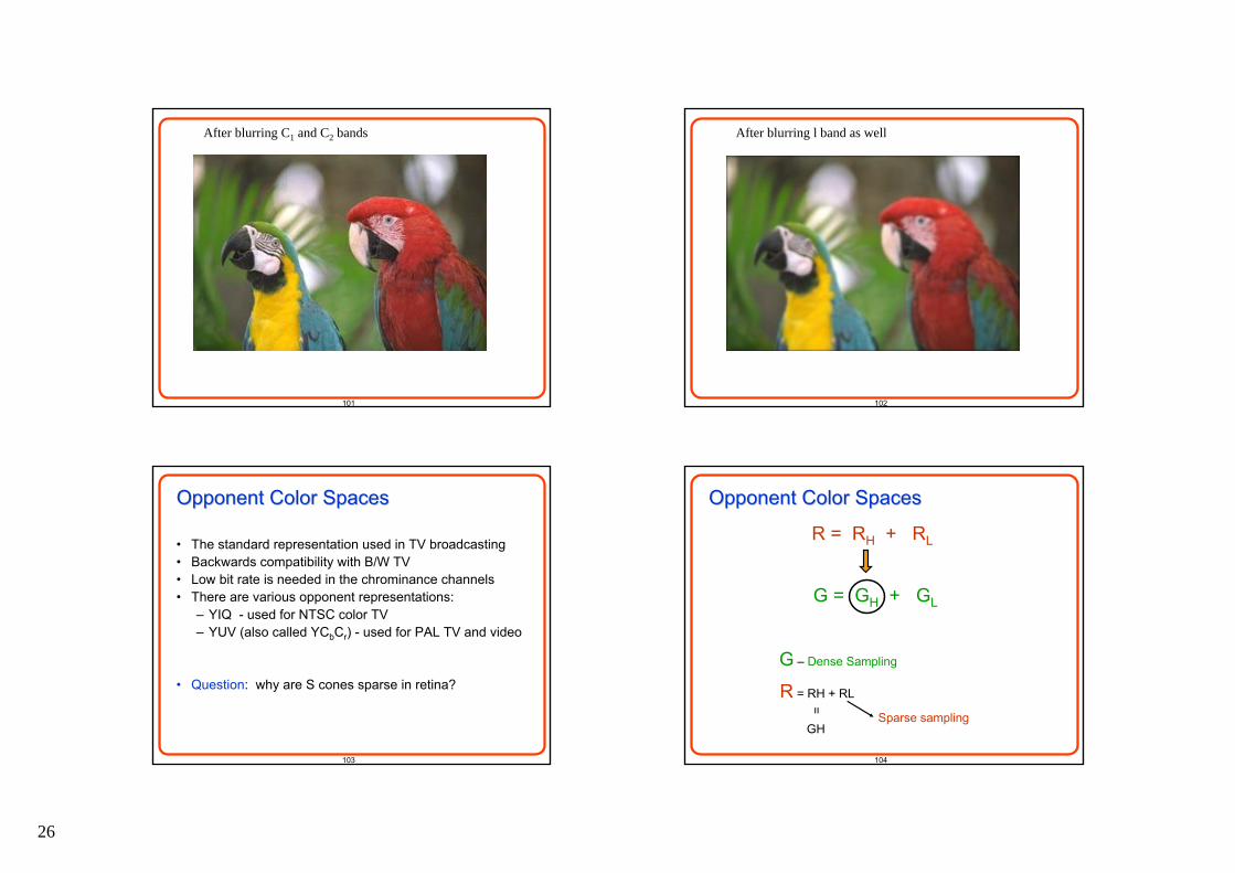
101
After blurring C1 and C2 bands
102
After blurring l band as well
103
Opponent Color SpacesOpponent Color Spaces
• The standard representation used in TV broadcasting• Backwards compatibility with B/W TV• Low bit rate is needed in the chrominance channels• There are various opponent representations:
– YIQ - used for NTSC color TV – YUV (also called YCbCr) - used for PAL TV and video
• Question: why are S cones sparse in retina?
104
Opponent Color SpacesOpponent Color Spaces
R = RH + RL
G = GH + GL
Sparse sampling
G – Dense Sampling
R = RH + RL
=
GH
27
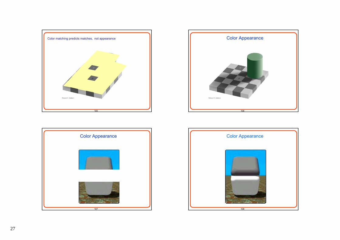
105
Color matching predicts matches, not appearanceColor matching predicts matches, not appearance
106
Color Appearance
107
Color Appearance
108
Color Appearance
28
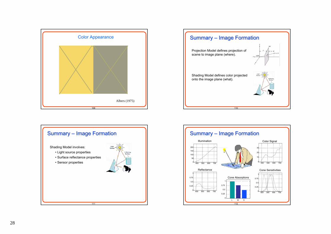
109
Color Appearance
Albers (1975)
110
Summary Summary –– Image FormationImage Formation
Projection Model defines projection ofscene to image plane (where).
Shading Model defines color projectedonto the image plane (what).
111
Summary Summary –– Image FormationImage Formation
Shading Model involves:• Light source properties• Surface reflectance properties• Sensor properties
112
Summary Summary –– Image FormationImage Formation
0
0.25
0.5
0.75
1
L M S
Cone Absorptions
Reflectance
Illumination Color Signal
Cone Sensitivities
400 500 600 7000
0.25
0.5
0.75
1
400 500 600 7000
10
20
30
400 500 600 7000
50
100
150
200
400 500 600 7000
0.25
0.5
0.75
1