Scanning Force Microscopy: Imaging & Cellular...

Fakultät für Physik und Geowissenschaften

Biophysics Lab Course WS 2012/13

Scanning Force MicroscopyImaging & Cellular Elasticity

:

Steve PawlizakRoom: 132Phone: (0341) 97 32713E-Mail: [email protected]

Linnéstraße 5, 04103 LeipzigFax: (0341) 97 32479www.uni-leipzig.de/~pwm

Tutors:

50 µm

100 µm

100µm

(Imag

e: S

teve

Paw

lizak

, 200

8)Abteilung:Physik der weichen Materie(Soft Matter Physics)

Institut fürExperimentelle Physik I

Prof. Dr. Josef A. Käs

Institute forExperimental Physics I Thomas Fuhs

Room: 115Phone: (0341) 97 32486E-Mail: [email protected]

Biophysics Lab Course Scanning Force Microscopy: Imaging & Cellular Elasticity

This lab experiment gives an introduction into scanning force microscopy (SFM) and demon-strates one of its biophysical applications as a tool for studying elastic properties (rheology)of biological cells, especially of their cytoskeleton. The understanding of material properties ofcells is an essential precondition to investigate the interplay between mechanics and biochemistry,which regulates cell functions and cell behavior.Scanning force microscopy – known from surface analysis of solid state bodies – uses the can-tilever, a microscopical leaf spring with a tip at its end, to probe a sample on nanometer scalemechanically.In this lab experiment, the material constants of a cantilever are to be determined first. Subse-quently, the local height and elasticity of cells shall be measured. The elasticity will be evaluatedusing the Hertz model.

Preparation for this Experiment:Before starting with the experiments, there will be a short pre-lab test to ensure that you arewell prepared. That is why, you should:

• read this tutorial thoroughly and additionally you may have a look at the given referenceliterature.

• inform yourself about cell biological background, especially about components of a celland the cytoskeleton (e.g. biophysics lecture, www.softmatterphysics.com, Wikipedia).

• inform yourself about phase contrast microscopy.

Bring a USB stick for storing your data that you will collect during your measurements.

Experimental and Analysis Tasks:Adjust the scanning unit (mounting the cantilever) and approach the cantilever onto thesample.

1. Determine the cantilever’s material constants (sensitivity 𝑠 and spring constant 𝑘).

2. Image two cells using phase contrast microscopy and scanning force microscopy. Recordheight- and error-image. Create 3D views and cross-sections.

3. Determine the tilt angle of the substrate plane for two cells with respect to the horizontalplane (𝑧 = 0).

4. Determine the local height of two cells at different positions on the cell surface (at least 5points for each cell).

5. Determine the local elasticity 𝐾 of two cells at different positions on the cell surface (atleast 5 points for each cell). Compare this to the elasticity of the glass surface. If it isreasonable, you might calculate a mean elasticity �̄�.

6. Compare your trace and retrace curves. Compare your trace curves on glass to those onthe cell surface. Describe the differences and explain where they come from.

To conclude this experiment and to get a grade, you are supposed to hand in a protocol whichshould contain the well-known sections: background and theory, materials and method (exper-imental techniques), execution of measurements (summary of the experiments you have done),data analysis and discussion of results, and error sources. Include the taken pictures and givedetailed figure captions. Since there will not be any final oral examination, your grade willstrongly depend on the quality of your protocol, but also on your preparation (pre-lab test) andexperimental skills.

2

www.softmatterphysics.com


1 General InformationThe precursor to the scanning force microscope (SFM), the scanning tunneling microscope, wasdeveloped by Binnig and Rohrer in the early 1980s und earned them the Nobel Prize forPhysics in 1986. The first SFM was invented by Binnig, Quate and Gerber in 1986. TheSFM is also known as atomic force microscope (AFM) which refers to the interactions betweenprobe and sample on the atomic level. The attractive Van-der-Waals-forces and repellentelectric charges (Pauli-repulsion) can be described by the Lennard-Jones potential.There are two main applications for scanning force microscopy:

• imaging samples with up to nanometer resolution (see section 3)

• measuring forces in the piconewton regime (see section 4)

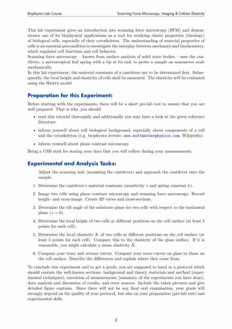
chip

cantilever

tip with bead

(a) Schematic representation

0.5 mm

(b) Image by reflected-light microscopy

Figure 1: Commercial cantilever, consisting of chip and leaf spring with tip, modified by gluing a 6 µmpolystyrene bead onto the tip. (Images taken from diploma thesis of Steve Pawlizak, 2009.)

2 Assembly (JPK NanoWizard® BioAFM)The core piece of an SFM is a soft elastic leaf spring, the cantilever (see front page). It extendsfrom an approximately 4 mm long chip, shown in Fig. 1. At its very end it has a sharp pyramidaltip. As soon as the cantilever comes very close to the sample or substrate, the leaf spring bends,i.e. the tip is moved upward or downward due to its interaction with the sample. This bendingis detected with high precision by a laser beam which is directed onto the cantilever and reflectedonto a position-sensitive four-quadrant photodiode (see Fig. 2). Initially, the laser spot is alignedto the center of the diode. When the cantilever bends, the reflection angle of the laser changesand the laser spot moves on the diode, which is measured as a change of the photo voltage calleddeflection 𝑢C of the cantilever.Cantilever, laser, and photodiode are mounted on the SFM scanning unit (SFM head). The SFMhead is placed on the microscope table over the sample. It can be moved in three dimensionsby a set of piezoelectrical elements1. A computer is connected via a controller box to the SFMhead for adjusting the piezo positions, data collection and analysis.Our SFM setup, the JPK NanoWizard® BioAFM (JPK Instruments, Berlin), has the greatadvantage of permitting the simultaneous usage of a variety of light microscopy techniques (e.g.phase contrast) together with the SFM. This is especially helpful for biological research.To avoid damaging living cells during the measurement and in order to have a well-definedgeometrical shape of the probe for the calculation of the elastic moduli, we glue a polystyrenebead (𝑑 = 6 µm) to the tip of the cantilever.

1A piezoelectric element is a device made from a material (crystals or ceramics) that expands or contracts indirect proportion to an applied electric field. They are used for precise movement and positioning.

3


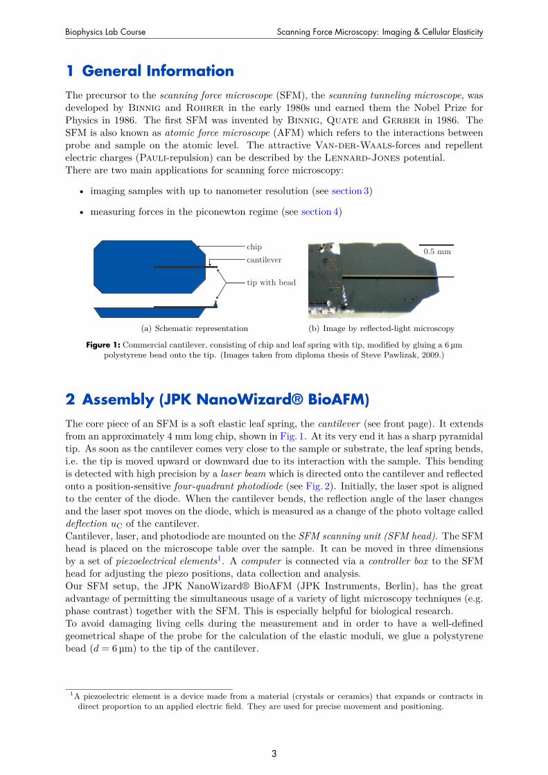
A B

C D

quadrantphotodiode

laser

cantilever chip (mountedon the AFM glass block)

verticallydeflectedcantilever

sample (e.g. cell)

substrate (e.g. coverslip)

AFM controller

heightadjustmentvia z-piezo

reflectionoff center

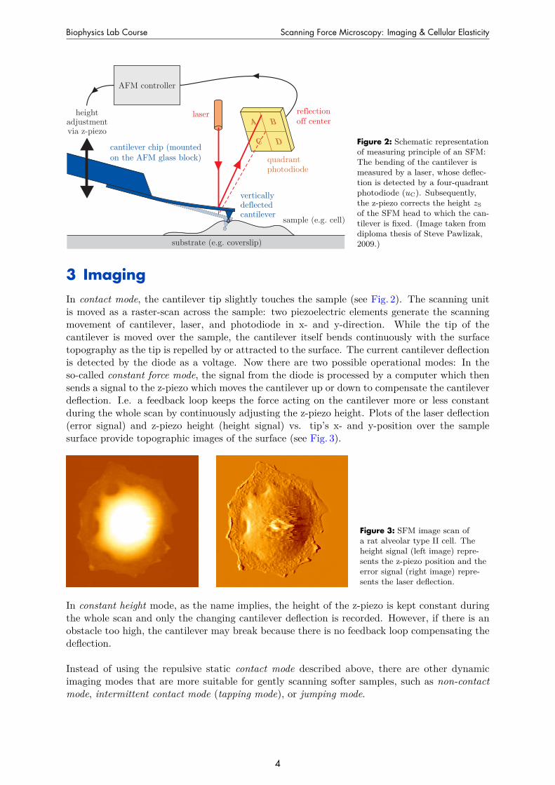
Figure 2: Schematic representationof measuring principle of an SFM:The bending of the cantilever ismeasured by a laser, whose deflec-tion is detected by a four-quadrantphotodiode (𝑢C). Subsequently,the z-piezo corrects the height 𝑧Sof the SFM head to which the can-tilever is fixed. (Image taken fromdiploma thesis of Steve Pawlizak,2009.)

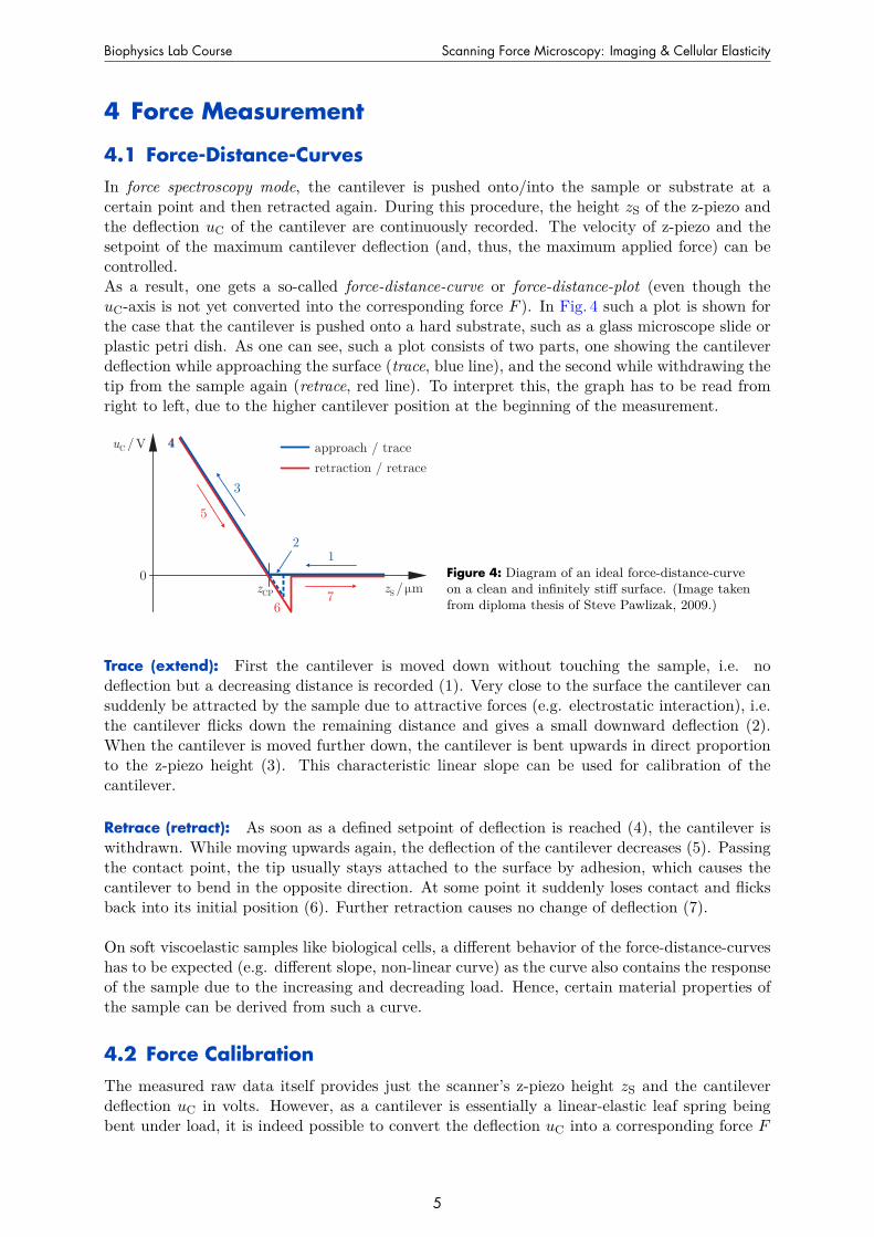
3 ImagingIn contact mode, the cantilever tip slightly touches the sample (see Fig. 2). The scanning unitis moved as a raster-scan across the sample: two piezoelectric elements generate the scanningmovement of cantilever, laser, and photodiode in x- and y-direction. While the tip of thecantilever is moved over the sample, the cantilever itself bends continuously with the surfacetopography as the tip is repelled by or attracted to the surface. The current cantilever deflectionis detected by the diode as a voltage. Now there are two possible operational modes: In theso-called constant force mode, the signal from the diode is processed by a computer which thensends a signal to the z-piezo which moves the cantilever up or down to compensate the cantileverdeflection. I.e. a feedback loop keeps the force acting on the cantilever more or less constantduring the whole scan by continuously adjusting the z-piezo height. Plots of the laser deflection(error signal) and z-piezo height (height signal) vs. tip’s x- and y-position over the samplesurface provide topographic images of the surface (see Fig. 3).

Figure 3: SFM image scan ofa rat alveolar type II cell. Theheight signal (left image) repre-sents the z-piezo position and theerror signal (right image) repre-sents the laser deflection.

In constant height mode, as the name implies, the height of the z-piezo is kept constant duringthe whole scan and only the changing cantilever deflection is recorded. However, if there is anobstacle too high, the cantilever may break because there is no feedback loop compensating thedeflection.

Instead of using the repulsive static contact mode described above, there are other dynamicimaging modes that are more suitable for gently scanning softer samples, such as non-contactmode, intermittent contact mode (tapping mode), or jumping mode.

4


4 Force Measurement

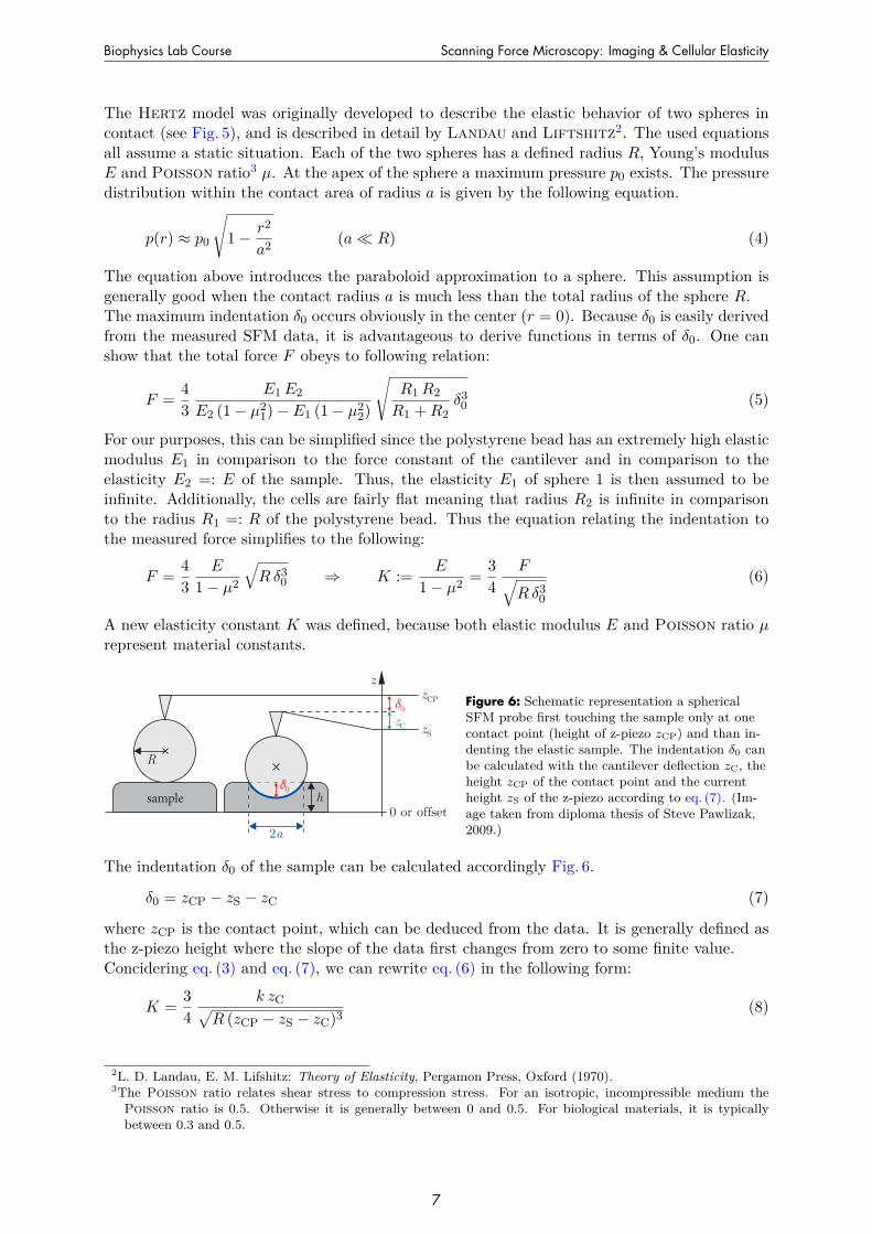
4.1 Force-Distance-CurvesIn force spectroscopy mode, the cantilever is pushed onto/into the sample or substrate at acertain point and then retracted again. During this procedure, the height 𝑧S of the z-piezo andthe deflection 𝑢C of the cantilever are continuously recorded. The velocity of z-piezo and thesetpoint of the maximum cantilever deflection (and, thus, the maximum applied force) can becontrolled.As a result, one gets a so-called force-distance-curve or force-distance-plot (even though the𝑢C-axis is not yet converted into the corresponding force 𝐹 ). In Fig. 4 such a plot is shown forthe case that the cantilever is pushed onto a hard substrate, such as a glass microscope slide orplastic petri dish. As one can see, such a plot consists of two parts, one showing the cantileverdeflection while approaching the surface (trace, blue line), and the second while withdrawing thetip from the sample again (retrace, red line). To interpret this, the graph has to be read fromright to left, due to the higher cantilever position at the beginning of the measurement.

0

uC /V

zS /µm

retraction / retrace

approach / trace

12

3

5

4

67

4

zCP

Figure 4: Diagram of an ideal force-distance-curveon a clean and infinitely stiff surface. (Image takenfrom diploma thesis of Steve Pawlizak, 2009.)

Trace (extend): First the cantilever is moved down without touching the sample, i.e. nodeflection but a decreasing distance is recorded (1). Very close to the surface the cantilever cansuddenly be attracted by the sample due to attractive forces (e.g. electrostatic interaction), i.e.the cantilever flicks down the remaining distance and gives a small downward deflection (2).When the cantilever is moved further down, the cantilever is bent upwards in direct proportionto the z-piezo height (3). This characteristic linear slope can be used for calibration of thecantilever.

Retrace (retract): As soon as a defined setpoint of deflection is reached (4), the cantilever iswithdrawn. While moving upwards again, the deflection of the cantilever decreases (5). Passingthe contact point, the tip usually stays attached to the surface by adhesion, which causes thecantilever to bend in the opposite direction. At some point it suddenly loses contact and flicksback into its initial position (6). Further retraction causes no change of deflection (7).

On soft viscoelastic samples like biological cells, a different behavior of the force-distance-curveshas to be expected (e.g. different slope, non-linear curve) as the curve also contains the responseof the sample due to the increasing and decreading load. Hence, certain material properties ofthe sample can be derived from such a curve.

4.2 Force CalibrationThe measured raw data itself provides just the scanner’s z-piezo height 𝑧S and the cantileverdeflection 𝑢C in volts. However, as a cantilever is essentially a linear-elastic leaf spring beingbent under load, it is indeed possible to convert the deflection 𝑢C into a corresponding force 𝐹

5


using only two material constants.

Recording a force-distance-curve on a substrate that appears to be infinitely hard in comparisonto the bending stiffness of the cantilever produces a characteristic graph, as shown in Fig. 4.This graph describes only the deflection behavior of the cantilever depending on the movementof the z-piezo, and it does not contain any information about the substrate itself. In fact, thelinear relationship can be used to determine a material constant called the sensitivity 𝑠 of thecantilever:

𝑠 := − 1slope = − ∆𝑧S

∆𝑢C[𝑠] = nm

V (1)

Knowing the sensitivity 𝑠, one can easily convert the cantilever deflection 𝑢C into a correspondinglength value:

𝑧C = 𝑠 𝑢C (2)

In the range of linear-elastic bending of the cantilever, Hook’s law is valid, relating the length𝑧C to the applied force 𝐹 via the cantilever’s spring constant 𝑘:

𝐹 = 𝑘 𝑧C [𝑘] = mNm (3)

However, a reliable calibration of 𝑘 is necessary to calculate 𝐹 . There are several methods to dothis. One approach is to calculate a theoretical spring constant based on the exact dimensionof the leaf spring measured by electron microscopy and material properties. Another approachis to push the cantilever against very stiff substrate and then against a softer known referencespring. The unknown 𝑘 is then calculated by rule of proportion from the ratio of the accordingsensitivity values. A third approach is based on adding masses to the cantilever and measureits deflection due to gravity.Our method of choice is the so-called thermal noise technique which is already implemented intoour SFM software and fully automated. In brief, the software measures the thermal fluctuationsof the free cantilever over time. Fourier transformation of the noise data yields the powerspectrum showing the resonance peak of the cantilever. This peak is fitted with a Lorenz curve.The area under this curve corresponds to

⟨︀𝑧2⟩︀

which is proportial to the energy 𝐸 = 12𝑘

⟨︀𝑧2⟩︀

of a harmonic oscillator. According to the equipartition theorem, this energy is equal to thethermal energy 𝐸 = 1

2𝑘B𝑇 . With these two equations, the spring constant 𝑘 can be calculated.

5 Analysis (Hertz Model)In our case, the main reason for doing force measurements is to obtain information about theelastic (or viscoelastic) properties of biological cells. A measure for elasticity is the elasticmodulus 𝐸 (Young’s modulus). The so-called Hertz model is commonly used to derive 𝐸 fromSFM indentation experiments.

z

r0

d ( )r2

d ( )r1

R1

R2

2a

Figure 5: Schematic represen-tation of two elastic spheres(radii 𝑅1, 𝑅2) touching ea-chother. The contact area hasa diameter of 2𝑎. The localindentations 𝛿1, 𝛿2 dependon the distance 𝑟 to the cen-ter (apex). (Image by StevePawlizak, 2009.)

6


The Hertz model was originally developed to describe the elastic behavior of two spheres incontact (see Fig. 5), and is described in detail by Landau and Liftshitz2. The used equationsall assume a static situation. Each of the two spheres has a defined radius 𝑅, Young’s modulus𝐸 and Poisson ratio3 𝜇. At the apex of the sphere a maximum pressure 𝑝0 exists. The pressuredistribution within the contact area of radius 𝑎 is given by the following equation.

𝑝(𝑟) ≈ 𝑝0

√︃1 − 𝑟2

𝑎2 (𝑎 ≪ 𝑅) (4)

The equation above introduces the paraboloid approximation to a sphere. This assumption isgenerally good when the contact radius 𝑎 is much less than the total radius of the sphere 𝑅.The maximum indentation 𝛿0 occurs obviously in the center (𝑟 = 0). Because 𝛿0 is easily derivedfrom the measured SFM data, it is advantageous to derive functions in terms of 𝛿0. One canshow that the total force 𝐹 obeys to following relation:

𝐹 = 43

𝐸1 𝐸2𝐸2 (1 − 𝜇2

1) − 𝐸1 (1 − 𝜇22)

√︃𝑅1 𝑅2

𝑅1 + 𝑅2𝛿3

0 (5)

For our purposes, this can be simplified since the polystyrene bead has an extremely high elasticmodulus 𝐸1 in comparison to the force constant of the cantilever and in comparison to theelasticity 𝐸2 =: 𝐸 of the sample. Thus, the elasticity 𝐸1 of sphere 1 is then assumed to beinfinite. Additionally, the cells are fairly flat meaning that radius 𝑅2 is infinite in comparisonto the radius 𝑅1 =: 𝑅 of the polystyrene bead. Thus the equation relating the indentation tothe measured force simplifies to the following:

𝐹 = 43

𝐸

1 − 𝜇2

√︁𝑅 𝛿3

0 ⇒ 𝐾 := 𝐸

1 − 𝜇2 = 34

𝐹√︁𝑅 𝛿3

0

(6)

A new elasticity constant 𝐾 was defined, because both elastic modulus 𝐸 and Poisson ratio 𝜇represent material constants.

z

δ0

zC

zCP

zS

R

2a

δ0

h

0 or offset

sample

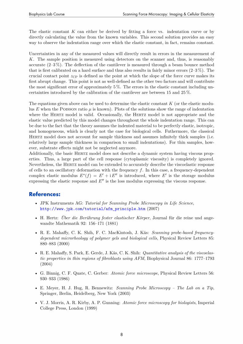
Figure 6: Schematic representation a sphericalSFM probe first touching the sample only at onecontact point (height of z-piezo 𝑧CP) and than in-denting the elastic sample. The indentation 𝛿0 canbe calculated with the cantilever deflection 𝑧C, theheight 𝑧CP of the contact point and the currentheight 𝑧S of the z-piezo according to eq. (7). (Im-age taken from diploma thesis of Steve Pawlizak,2009.)

The indentation 𝛿0 of the sample can be calculated accordingly Fig. 6.

𝛿0 = 𝑧CP − 𝑧S − 𝑧C (7)

where 𝑧CP is the contact point, which can be deduced from the data. It is generally defined asthe z-piezo height where the slope of the data first changes from zero to some finite value.Concidering eq. (3) and eq. (7), we can rewrite eq. (6) in the following form:

𝐾 = 34

𝑘 𝑧C√︀𝑅 (𝑧CP − 𝑧S − 𝑧C)3 (8)

2L. D. Landau, E. M. Lifshitz: Theory of Elasticity, Pergamon Press, Oxford (1970).3The Poisson ratio relates shear stress to compression stress. For an isotropic, incompressible medium the

Poisson ratio is 0.5. Otherwise it is generally between 0 and 0.5. For biological materials, it is typicallybetween 0.3 and 0.5.

7


The elastic constant 𝐾 can either be derived by fitting a force vs. indentation curve or bydirectly calculating the value from the known variables. This second solution provides an easyway to observe the indentation range over which the elastic constant, in fact, remains constant.

Uncertainties in any of the measured values will directly result in errors in the measurement of𝐾. The sample position is measured using detectors on the scanner and, thus, is reasonablyaccurate (2–3 %). The deflection of the cantilever is measured through a beam bounce methodthat is first calibrated on a hard surface and thus also results in fairly minor errors (2–3 %). Thecrucial contact point 𝑧CP is defined as the point at which the slope of the force curve makes itsfirst abrupt change. This point is not as well-defined as the other two factors and will contributethe most significant error of approximately 5 %. The errors in the elastic constant including un-certainties introduced by the calibration of the cantilever are between 15 and 25 %.

The equations given above can be used to determine the elastic constant 𝐾 (or the elastic modu-lus 𝐸 when the Poisson ratio 𝜇 is known). Plots of the solutions show the range of indentationwhere the Hertz model is valid. Occasionally, the Hertz model is not appropriate and theelastic value predicted by this model changes throughout the whole indentation range. This canbe due to the fact that the theory assumes the indented material to be perfectly elastic, isotropic,and homogeneous, which is clearly not the case for biological cells. Futhermore, the classicalHertz model does not account for sample thickness and assumes infinitely thick samples (i.e.relatively large sample thickness in comparison to small indentations). For thin samples, how-ever, substrate effects might not be neglected anymore.Additionally, the basic Hertz model does not describe a dynamic system having viscous prop-erties. Thus, a large part of the cell response (cytoplasmic viscosity) is completely ignored.Nevertheless, the Hertz model can be extended to accurately describe the viscoelastic responseof cells to an oscillatory deformation with the frequency 𝑓 . In this case, a frequency-dependentcomplex elastic modulus 𝐸*(𝑓) = 𝐸′ + i 𝐸′′ is introduced, where 𝐸′ is the storage modulusexpressing the elastic response and 𝐸′′ is the loss modulus expressing the viscous response.

References:• JPK Instruments AG: Tutorial for Scanning Probe Microscopy in Life Science,

http://www.jpk.com/tutorial/afm_principle.htm (2007)

• H. Hertz: Über die Berührung fester elastischer Körper, Journal für die reine und ange-wandte Mathematik 92: 156–171 (1881)

• R. E. Mahaffy, C. K. Shih, F. C. MacKintosh, J. Käs: Scanning probe-based frequency-dependent microrheology of polymer gels and biological cells, Physical Review Letters 85:880–883 (2000)

• R. E. Mahaffy, S. Park, E. Gerde, J. Käs, C. K. Shih: Quantitative analysis of the viscoelas-tic properties in thin regions of fibroblasts using AFM, Biophysical Journal 86: 1777–1793(2004)

• G. Binnig, C. F. Quate, C. Gerber: Atomic force microscope, Physical Review Letters 56:930–933 (1986)

• E. Meyer, H. J. Hug, R. Bennewitz: Scanning Probe Microscopy – The Lab on a Tip,Springer, Berlin, Heidelberg, New York (2003)

• V. J. Morris, A. R. Kirby, A. P. Gunning: Atomic force microscopy for biologists, ImperialCollege Press, London (1999)

8

http://www.jpk.com/tutorial/afm_principle.htm


6 Hints for Data Analysis

6.1 Light Microscopy ImagesMicroscope images (*.jpg) taken by a CCD camera are meaningless without a scale bar whichindicates the size of the shown objects. To include a scale bar, the actual magnification orresolution of the used imaging assembly has to be determined. This can be done by takinga reference image of a microscope slide with 10 µm scale (grating with 2 mm total length and0.01 mm interval width) using the very same combination of camera, objective and cameramount. Afterwards, the corresponding number of pixels in the graphic file is counted with anyimage processing software.

6.2 SFM Image ScansSFM image scans are saved in a proprietary JPK file format (*.jpk) and have to be post-processed to create common graphic files like JPEG (*.jpg). After your experiments you willhave time to create different cross-sections and 3d views using the “JPK SPM Data Processing”software. If you want to edit your JPK files at home, you could use “Gwyddion”, which is anopen source software for SPM data visualization and analysis. Windows- and Linux-versionscan be downloaded for free from http://gwyddion.net/.Do not forget to include some important scan parameters (IGain, PGain, setpoint, line rate,scan size, scan resolution in pixel) into your protocol.

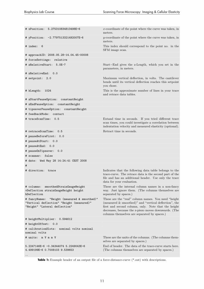
6.3 Force-Distance-CurvesForce-distance-curves are saved in a proprietary JPK file format (*.jpk-force). Using the batchscript jpk-force-legacy-export, they must be converted into plain ASCII text files (*.out) whichcan be imported into any scientific graphing and data analysis software you like (e.g. ORIGIN).Each text file has two sections, first one with the data of the trace curve and the second one withthe data of the retrace curve. You can use the splitforcefile script to create separate text filesfor trace and retrace curves. For your analysis, the columns “height (measured & smoothed)”and “vertical deflection” of the trace curves are of interest only.Every output file has a defined header containing some important parameters of the relatedforce-distance-curve like relative setpoint, index and 𝑥-𝑦-position. Especially, relative setpoint,z-length and scan time should be mentioned in your protocol. Tab. 1 shows an example header.

6.4 Evaluation StepsA. Find the contact points of the glass curves

1. Plot “vertical deflection” 𝑢C vs. “height (measured & smoothed)” 𝑧S.

2. Remove the offset in the vertical deflection 𝑢C.

3. Plot offset-corrected “vertical deflection” 𝑢C vs. “height (measured & smoothed)” 𝑧S.

4. Fit the linear part of the curve and determine the point of intersection with the height-axis.This gives you the 𝑧-component of your position vector �⃗�𝑖.

5. Determine the plane through three contact points and calculate its tilt angle towards thenormal plane with �⃗� = (0, 0, 1).

9

http://gwyddion.net/


B. Determine the local cell heights

1. Plot “vertical deflection” 𝑢C vs. “height (measured & smoothed)” 𝑧S.

2. Remove the offset in the vertical deflection 𝑢C.

3. Plot offset-corrected “vertical deflection” 𝑢C vs. “height (measured & smoothed)” 𝑧S.

4. Read contact point from the graph. This gives you the 𝑧-component of your positionvector �⃗�𝑖.

5. Now you have the substrate plane and some cell surface vectors. Calculate the the distancebetween the cell surface and the plane.

C. Determine the local cell elasticities

1. Convert the height-axis into indentation 𝛿0 using equ. (7) and convert the vertical deflectioninto force 𝐹 using equ. (3).

2. Plot 𝐹 2/3 vs. 𝛿0 to see if you have a linear range where the Hertz model applies.

3. To determine 𝐾 either fit the linear range in 𝐹 2/3-𝛿0-diagram or fit the Hertz model tothe curve in 𝐹 -𝛿0-diagram.

4. Additionally, you may plot 𝐾 vs. 𝛿0 using equ. (6) to check in which range 𝐾 actuallyremains constant during the indentation.

For each evaluation step, you should include the graphs with fittings and the equations forcalculations into your protocol. It is not sufficient to state only the final results (tilt angle,height and elasticity).

10


# xPosition: 5.275310834813498E-6 𝑥-coordinate of the point where the curve was taken, inmeters.

# yPosition: -2.7797513321492007E-6 𝑦-coordinate of the point where the curve was taken, inmeters.

# index: 6 This index should correspond to the point no. in theSFM image scan.

# approachID: 2008.05.28-14.04.45-00008

# forceSettings: relative

# zRelativeStart: 5.0E-7 Start−End gives the z-Length, which you set in theparameters, in meters.

# zRelativeEnd: 0.0

# setpoint: 2.0 Maximum vertical deflection, in volts. The cantileverbends until its vertical deflection reaches this setpointyou chose.

# kLength: 1024 This is the approximate number of lines in your traceand retrace data tables.

# zStartPauseOption: constantHeight

# zEndPauseOption: constantHeight

# tipsaverPauseOption: constantHeight

# feedbackMode: contact

# traceScanTime: 0.5 Extand time in seconds. If you tried different tracescan times, you could investigate a correlation betweenindentation velocity and measured elasticity (optional).

# retraceScanTime: 0.5 Retract time in seconds.# pauseBeforeFirst: 0.0

# pauseAtStart: 0.0

# pauseAtEnd: 0.0

# pauseOnTipsaver: 0.0

# scanner: false

# date: Wed May 28 14:24:41 CEST 2008

#

# direction: trace Indicates that the following data table belongs to thetrace-curve. The retrace data is the second part of thefile and has an additional header. Use only the tracedata for your evaluation.

# columns: smoothedStrainGaugeHeightvDeflection strainGaugeHeight heighthDeflection

These are the internal column names in a non-fancyway. Just ignore them. (The columns themselves areseparated by spaces.)

# fancyNames: "Height (measured & smoothed)""Vertical deflection" "Height (measured)""Height" "Lateral deflection"

These are the “real” column names. You need “height(measured & smoothed)” and “vertical deflection”, thefirst and second column, only. Note that the heightdecreases, because the z-piezo moves downwards. (Thecolumns themselves are separated by spaces.)

# heightMultiplier: 0.594612

# heightOffset: 0.0

# calibrationSlots: nominal volts nominalnominal volts

# units: m V m m V These are the units of the columns. (The columns them-selves are separated by spaces.)

5.2247146E-6 -0.34344074 5.2249043E-64.499199E-6 0.7008103 9.539653

End of header. The data of the trace-curve starts here.(The columns themselves are separated by spaces.)

...Table 1: Example header of an output file of a force-distance-curve (*.out) with descriptions.

11

Scanning Force Microscopy: Imaging & Cellular...

Documents

Transcript of Scanning Force Microscopy: Imaging & Cellular...