
Prairie Hydrological Model Study - usask.ca · Prairie Hydrological Model Study ... impacts...
126
i Prairie Hydrological Model Study Final Report Centre for Hydrology Report No. 7 John Pomeroy, Xing Fang, Cherie Westbrook, Adam Minke, Xulin Guo, and Tom Brown Centre for Hydrology University of Saskatchewan 117 Science Place Saskatoon, SK S7N 5C8 January, 2010 Centre for Hydrology Report #7
Transcript of Prairie Hydrological Model Study - usask.ca · Prairie Hydrological Model Study ... impacts...

i
Prairie Hydrological Model Study Final Report
Centre for Hydrology Report No. 7 John Pomeroy, Xing Fang, Cherie Westbrook, Adam Minke, Xulin Guo, and Tom Brown
Centre for Hydrology University of Saskatchewan
117 Science Place Saskatoon, SK
S7N 5C8
January, 2010
Centre for Hydrology Report #7

ii
Prairie Hydrological Model Study Final Report
- By -
John Pomeroy, Xing Fang, Cherie Westbrook, Adam Minke, Xulin Guo, and Tom Brown
© Centre for Hydrology, University of Saskatchewan,
Saskatoon, Saskatchewan January, 2010

i
Executive Summary This report describes the development of the Prairie Hydrological Model (PHM), a model that is suitable for hydrological process simulations in the prairie pothole region of Western Canada. The model considers all major prairie hydrological cycle, wetland storage, and runoff generation mechanisms and is capable of addressing the influences of changing land use, wetland drainage and climate variability. The purpose of this report is to describe the model, examine the performance of the model, and to demonstrate the model as a predictive tool for prairie hydrology. This purpose is achieved by using the model to analyze the impacts of wetland drainage and restoration as well as changes in surrounding upland land use on downstream hydrology. This focus on wetland drainage impacts required the development and testing of a new volume-area-depth (v-a-h) method for estimating wetland volume in the prairie pothole region. The method was incorporated into the PHM and improved the model’s ability to estimate wetland volume. The Cold Regions Hydrological Model platform (CRHM) is a computational toolbox developed by the University of Saskatchewan to set up and run physically based, flexible, object oriented hydrological models. CRHM was used to create the PHM for Smith Creek Research Basin (~400 km2), Saskatchewan. Two types of PHM runs were performed to estimate the basin hydrology. The non-LiDAR (Light Detection and Ranging) runs used a photogrammetric based DEM (digital elevation model) to estimate drainage area and hydrograph calibration to determine maximum depressional storage. The LiDAR runs used a fine-scale LiDAR derived DEM to determine drainage area and maximum depressional storage; use of LiDAR information meant that calibration was not required to set any parameter value. In both cases all non-topographic parameters were determined from basin observations, remote sensing and field surveys. Both LiDAR and non-LiDAR model predictions of winter snow accumulation were very similar and compared quite well with the distributed snow survey results. The simulations were able to effectively capture the natural sequence of snow redistribution and relocate snow from ‘source’ areas (e.g. fallow and stubble fields) to ‘sink’ or ‘drift’ areas (e.g. tall vegetated wetland area and deeply incised channels). This is a vital process in controlling the water balance of prairie basins as most water in wetlands and prairie river channels is the result of redistribution of snow by wind and subsequent snowmelt runoff. Soil moisture status is an important factor in determining the spring surface runoff and in controlling agricultural productivity. Unfrozen soil moisture content at a point during melt was adequately simulated from both modelling approaches. Both modelling approaches were capable of matching the spring streamflow hydrographs with good accuracy; the non-LiDAR approach performed slightly better than the LiDAR approach because the streamflow hydrograph was calibrated, whereas no calibration was involved in the LiDAR simulation. However, the LiDAR approach to simulation shows promise for application to ungauged basins or to changing basins and demonstrates that prairie hydrology can be simulated based on our current understanding of physical principles and good basin data that provides “real” parameters. The approach uses a

ii
LiDAR DEM, SPOT 5 satellite images and involved automated basin parameters delineation techniques and a new wetland depth-area-volume calculation. The new wetland depth-area-volume calculation used a LiDAR-derived DEM to estimate maximum depressional storage, a substantial improvement over estimates generated from simpler area-volume methods. This was likely due to the inclusion of information on depression morphology when calculating volume. Further, the process to retrieve the coefficients from a LiDAR DEM was automated and wetland storage was estimated at a broad spatial scale. A GIS model was created that can automatically extract the elevation and area data necessary for use in the new depth-area-volume method. Using the Prairie Hydrological Model, PHM, a series of scenarios on changing land use and wetland and drainage conditions was created from 2007-08 meteorological data. The scenario simulations were used to calculate cumulative spring basin discharge, total winter snow accumulation, blowing snow transport and sublimation, cumulative infiltration, and spring surface depression storage status. From these simulations, spring streamflow volumes decreased by 2% with complete conversion to agriculture and by 79% with complete restoration of wetlands; conversely it increased by 41% with complete conversion to forest cover and by 117% with complete wetland drainage. The greatest sensitivity was to further drainage of wetlands which substantially increased streamflow. Additional sensitivity analysis of scenarios on basin streamflow using historical (29-year periods: 1965-82 and 1993-2005) meteorology and initial conditions and current land use was carried out. Results showed that the effects of land use change and wetland drainage alteration on cumulative basin spring discharge volume and peak daily spring discharge were highly variable from year to year and depended on the flow condition. For both forest conversion and agricultural conversion and wetland drainage scenarios increased the long-term average peak discharge from current conditions, whereas wetland restoration reduced it. Forest conversion, agricultural conversion and wetland drainage scenarios increased the long-term average spring discharge volume by 1%, 19%, and 36% respectively; whilst the wetland restoration scenario reduced volumes by 45%. Several recommendations were made regarding the modelling challenges faced by this study and value of local meteorological data collection and using a LiDAR generated DEM for Prairie hydrological modelling purposes. It is recommended that similar studies be conducted in other geographic areas of the prairies where climate, soils, wetland configuration and drainage may produce differing results.

iii
Acknowledgements
The authors would like to thank Dr. Kevin Shook and Mr. Michael Solohub of the Centre for Hydrology for useful advice, discussion and assistance in field work. Funding was provided through Prairie Habitat Joint Venture Policy Committee, Agriculture and Agri-Food Canada, Prairie Provinces Water Board, Saskatchewan Watershed Authority, Manitoba Water Stewardship, Ducks Unlimited Canada, the Canada Research Chairs Programme, and the Drought Research Initiative (DRI), a network funded by the Canadian Foundation for Climate and Atmosphere Sciences (CFCAS). Various archived GIS data provided by Ducks Unlimited Canada, hydrometric data acquired by Water Survey of Canada, and historical soil moisture data provided by Manitoba Water Stewardship were essential to this research. The permission of Mr. Don Werle of Langenburg, Saskatchewan to have a meteorological station operated on his land is gratefully acknowledged. The cooperation and support of various land owners and producers in Smith Creek Research Basin and the support of the Smith Creek Advisory Committee and the Langenburg Regional Economic Development Authority made this study not only possible but pleasurable. We thank you all for your patience and good will.

iv

v
Table of Contents
Executive Summary …………………………………………………………………….. i Acknowledgements …………………………………………………………………….. iii List of Figures ………………………………………………………………………….. vii List of Tables …………………………………………………………………………… x 1 Introduction …………………………………………………………………….. 1 2 Literature Review on Canadian Prairie Hydrology ……………………………. 3
2.1 Prairie Hydrological Cycle ………………………………………………… 3 2.2 Prairie Runoff Generation …………………………………………………. 6 2.3 Land Cover and Wetland Effects on Prairie Hydrology …………………... 8
3 Study Site and Field Observations ……………………………………………. 11
3.1 Site Description …………………………………………………………… 11 3.2 Field Data Observations …………………………………………………... 12 3.3 LiDAR and non-LiDAR DEM ……………………………………………. 23 3.4 Remote Sensing of the Basin ……………………………………………… 23
4 Prairie Hydrological Model …………………………………………………… 25
4.1 Model Description ………………………………………………………… 25 4.2 Model Equations …………………………………………………………... 29
4.2.1 Snow Accumulation ……………………………………………... 29 4.2.2 Snowmelt ………………………………………………………... 32
4.2.3 Infiltration ……………………………………………………….. 35 4.2.4 Evaporation ……………………………………………………… 37
5 Modelling Parameterization Methods …………………………………………. 38
5.1 Determination and Estimation of Parameter ………………………………. 38 5.1.1 Sub-basin and HRU Determination ……………………………… 38 5.1.2 Basin Physiographic Parameters ………………………………… 39 5.1.3 Albedo and Canopy Parameters …………………………………. 39 5.1.4 Blowing Snow and Frozen Soil Parameters ……………………... 43 5.1.5 Routing Parameters ……………………………………………… 43 5.1.6 Wetland Module Parameters …………………………………….. 46
5.2 Simplified Volume-Area-Depth Method for Wetland Storage Estimation ... 52 5.2.1 Measurement of Actual Wetland Volume ……………………….. 52 5.2.2 Theory for Applying the Simplified V-A-h Method to a LiDAR DEM …………………………………………………………………… 52 5.2.3 LiDAR V-A-h Method …………………………………………... 53

vi
5.2.4 Automation of the LiDAR V-A-h Method ………………………. 55 5.2.5 Case Study ……………………………………………………….. 55 5.2.6 Comparison between LiDAR V-A-h and V-A Methods ………… 57
6 Modelling Results ……………………………………………………………… 58
6.1 Comparison between the Calibrated and Uncalibrated Simulations ………. 58 6.1.1 Winter Snowpack Prediction and Comparison …………………... 58 6.1.2 Spring Soil Moisture Prediction and Comparison ……………...... 69 6.1.3 Spring Streamflow Prediction and Comparison …………………. 70
6.2 Comparison of Wetland Storage Estimation using the LiDAR V-A-h and V-A Methods ………………………………………………………………………... 73
6.2.1 Assessing Volume Error for the Study Wetlands ………………... 73 6.2.2 Comparison between the LiDAR V-A-h to V-A Methods ………. 74
7 Sensitivity Analysis of Smith Creek Scenario Simulations …...……………….. 76
7.1 Scenario Description ……………………………………………………….. 76 7.1.1 2007-2008 Scenario Simulations …… ……………………….... 76 7.1.2 Historical Scenarios Simulations ………………………………… 77 7.2 Results of Scenario Simulations …………………………………………… 92 7.2.1 2007-2008 Scenario Simulations Results ……………………... 92 7.2.2 Historical Scenarios Simulations Results ………………………... 96
8 Conclusions and Recommendations …..……………………………………… 104
8.1 Conclusions ……………………………………………………………….. 104 8.2 Recommendations ………………………………………………………… 107
List of References …………………………………………………………………….. 108

vii
List of Figures Figure 1 Prairie hydrological cycle ……………………………………………………… 3 Figure 2 Non-contributing areas of drainage basins as delineated by PFRA …………… 7 Figure 3 Observed springtime water levels in pond 109, St. Denis NWA during 1997-
2005 ……………………………………………………………………………... 8 Figure 4 Water balance of Creighton Tributary of Bad Lake Basin, Saskatchewan …… 9 Figure 5 Study site ……………………………………………………………………... 11 Figure 6 Website daily weather summary for Smith Creek ……………………………. 12 Figure 7 Meteorological data during 31October 2007-30 April 2008 at Smith Creek SC-1
station …………………………………………………………………………... 14 Figure 8 Meteorological data during 31October 2008-1 May 2009 at Smith Creek SC-1
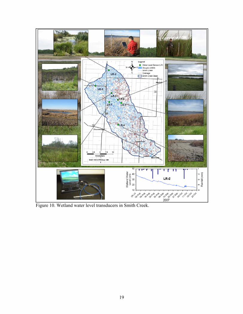
station ……………………………………………………………………………16 Figure 9 Rain gauge stations in Smith Creek ……………………………………………18 Figure 10 Wetland water level transducers in Smith Creek ……………………………. 19 Figure 11 Soil and vegetation surveys in Smith Creek ………………………………….20 Figure 12 Snow survey transects in Smith Creek ……………………………………….21 Figure 13 Historical data during 1975-2006 …………………………………………….22 Figure 14 DEMs …………………………………………………………………………23 Figure 15 SPOT 5 10-m multispectral images …………………………………………. 24 Figure 16 Flowchart of physically based hydrological modules for PHM …………….. 26 Figure 17 Flowchart of a wetland module of soil moisture balance calculation with
wetland or depression storage and fill-and-spill ………………………………...28 Figure 18 Cross-sectional view of control volume for blowing snow mass fluxes ……. 29 Figure 19 Cross-sectional view of control volume for snowmelt energies ……………. 33 Figure 20 CRHM modelling structure ………………………………………………… 39

viii
Figure 21 Pre-processing procedure for deriving sub-basins at Smith Creek Research Basin …………………………………………………………………………… 40
Figure 22 Pre-processing procedure for generating HRU classification at Smith Creek
Research Basin …………………………………………………………………. 41 Figure 23 Routing sequence …………………………………………………………… 46 Figure 24 Flowchart of an automated procedure used by the uncalibrated modelling for
estimating maximum surface depression storage ……………………………… 49 Figure 25 ArcGIS 3D “cut/fill” analysis ………………………………………………. 50 Figure 26 Generalized wetland illustrating area and depth measurements required for
applying the simplified V-A-h method to a LiDAR DEM ……………………... 53 Figure 27 Plan view of wetland S104 at SDNWA with relevant, closed contours (white),
and the contour representing the spill point of the wetland (grey) …………….. 54 Figure 28 SDNWA study site ………………………………………………………….. 56 Figure 29. Simulation of snow accumulation development for Smith Creek Research
Basin during 31 October 2007-30 April 2008 …………………………………. 59 Figure 30 Simulation of snow accumulation development for Smith Creek Research
Basin during 31 October 2008-30 April 2009 …………………………………. 61 Figure 31 Revised Simulation of snow accumulation development for Smith Creek
Research Basin during 31 October 2008-30 April 2009 ………………………. 64 Figure 32 Comparisons of the observed and simulated snow accumulation (SWE) during
2008 simulation period for seven HRUs in the sub-basin 1 of Smith Creek Research Basin …………………………………………………………………. 67
Figure 33 Comparisons of the observed and simulated snow accumulation (SWE) during
2009 simulation period for seven HRUs in the sub-basin 1 of Smith Creek Research Basin …………………………………………………………………. 68
Figure 34 Comparisons of the observed and simulated volumetric spring soil moisture
from the main weather station in the Smith Creek Research Basin …………… 70 Figure 35 Comparisons of the observed and simulated spring daily mean discharge in the
Smith Creek Research Basin ………………………………………………….. 71 Figure 36 Comparisons of the observed and simulated spring daily mean discharge in the
Smith Creek Research Basin using meteorological data from Yorkton ……… 73

ix
Figure 37 LiDAR V-A-h method error assessment …………………………………….. 74 Figure 38 Volume estimated through the LiDAR V-A-h method, Wiens method and
Gleason method ……………………………………….……………………….. 75 Figure 39 Development of Smith Creek current scenarios ……………………………. 78 Figure 40 Development of Smith Creek historical scenarios …………………………. 89 Figure 41 Scenarios of Smith Creek springtime basin discharge ……………………… 93 Figure 42 Scenarios of total winter snow accumulation at Smith Creek basin ……….. 93 Figure 43 Scenarios of total blowing snow transport at Smith Creek basin …………… 94 Figure 44 Scenarios of total blowing snow sublimation at Smith Creek basin …………94 Figure 45 Scenarios of total infiltration at Smith Creek basin ………………………… 95 Figure 46 Scenarios of total springtime surface depression storage at Smith Creek
basin ……………… …………………………………………………………... 95 Figure 47 Simulations of scenarios of Smith Creek cumulative spring discharge during 1965-82 and 1993-2005 periods ……………………………………………………… 98 Figure 48 Sensitivity of the Smith Creek cumulative spring discharge during 1965-82 and
1993-2005 periods ……………………………………………………………. 99 Figure 49 Effect of long-term land use and drainage change on Smith Creek cumulative
spring discharge ………………………………………………………………. 100 Figure 50 Simulations of scenarios of Smith Creek peak daily spring discharge during
1965-82 and 1993-2005 periods ……………………………………………… 101 Figure 51 Sensitivity of the Smith Creek peak daily spring discharge during 1965-82 and
1993-2005 periods ……………………………………………………………. 102 Figure 52 Effect of long-term land use and drainage change on Smith Creek peak daily
spring discharge ………………………………………………………………. 103

x
List of Tables Table 1 Blowing snow transport and sublimation losses for fallow and stubble fields of
1 km length in Saskatchewan …………………………………………………… 8 Table 2 Basin physiographic parameters ………………………………………………. 42 Table 3 Albedo and canopy parameters ………………………………………………... 42 Table 4 Blowing snow and frozen soil parameters …………………………………….. 43 Table 5 Parameters for runoff routing between HRUs within the sub-basins (RBs) ….. 44 Table 6 Routing distribution parameter between HRUs within the sub-basins (RBs) … 44 Table 7 Parameters for channel routing between the sub-basins (RBs) ……………….. 44 Table 8 Parameters of soil recharge layer, soil column, and subsurface and groundwater
drainage for the wetland module ………………………………………………. 46 Table 9 Parameters of surface depression storage for the wetland module …………… 48 Table 10 Evaluation of snowpack simulations ………………………………………… 69 Table 11 Evaluation of volumetric spring soil moisture predictions ………………….. 70 Table 12 Evaluation of simulating spring basin discharge …………………………….. 71 Table 13 Evaluation of simulating spring basin discharge using meteorological data from
Yorkton ………………………………………………………………………… 72 Table 14 Changes of HRU area, fall soil saturation, and sdmax for the scenarios of
‘complete forest cover’ at the initial stage ……………………………………... 79 Table 15 Changes of HRU area, fall soil saturation, and sdmax for the scenarios of
‘primarily agricultural land use’ at the initial stage ……………………………. 80 Table 16 Changes of HRU area, fall soil saturation, and sdmax for the scenarios of ‘high
natural wetland extent/poorly drained’ at the initial stage …………………....... 81 Table 17 Changes of HRU area, fall soil saturation, and sdmax for the scenarios of
‘minimal wetland extent/well drained’ at the initial stage …………………....... 82 Table 18 Changes of HRU area, fall soil saturation, and sdmax for the scenarios of
‘complete forest cover’ at the mature stage ……………………………………. 83

xi
Table 19 Changes of HRU area, fall soil saturation, and sdmax for the scenarios of ‘primarily agricultural land use’ at the mature stage …………………………... 84
Table 20 Changes of HRU area, fall soil saturation, and sdmax for the scenarios of ‘high
natural wetland extent/poorly drained’ at the mature stage …………………… 85 Table 21 Changes of HRU area, fall soil saturation, and sdmax for the scenarios of
‘minimal wetland extent/well drained’ at the mature stage ……………………. 86 Table 22 Changes of routing distribution parameter between HRUs within the sub-basins
for the scenarios of ‘high natural wetland extent/poorly drained’ at both initial and mature stages …………………………………………………………………… 87
Table 23 Changes of routing distribution parameter between HRUs within the sub-basins
for the scenarios of ‘minimal wetland extent/well drained’ at both initial and mature stages …………………………………………………………………… 88
Table 24 Changes of HRU area (km2) for historical scenarios of ‘forest conversion’,
‘agricultural conversion’, ‘wetland restoration’, and ‘wetland drainage’ ……… 90 Table 25 Changes of routing distribution parameter between HRUs within the sub-basins
for historical scenarios of ‘forest conversion’, ‘agricultural conversion’, ‘wetland restoration’, and ‘wetland drainage’ …………………………………………… 91

1
1. Introduction The Canadian Prairies cover the southern part of the provinces of Alberta, Saskatchewan, and Manitoba and are the northern limit of the North American Great Plains. The northern fringe of the Prairies is covered by Parkland, which was a mixed deciduous forest, wetland, and grassland complex that has been largely cultivated to cereal grains and oilseeds or converted to pasture since European settlement over 100 years ago. The Prairies are characterized by relatively low precipitation especially in the southwest part due to the atmospheric flow barrier imposed by the Rocky Mountains and experience frequent water deficits and low soil moisture reserves (Agriculture and Agri-Food Canada, 1998). Annual precipitation in the prairie region of Saskatchewan ranges from 300-400 mm (Pomeroy et al., 2007a), about one third of which occurs as snowfall (Gray and Landine, 1988). The Prairies are a cold region and exhibit classical cold regions hydrology with continuous snowcover and frozen soils over much of the region in the winter. Great variation in hydrology exists across the Prairies, with fairly well-drained, semi-arid basins in the southwest part and with many wetlands and lakes in the Parklands of the sub-humid north central and eastern parts. The hydrology of the central Prairies is characterized by: long periods of winter (usually 4-5 months) with occasional mid-winter melts
(frequent in the southwest and infrequent in the northeast), with the snowcover modified by wind redistribution and sublimation of blowing snow (Pomeroy et al., 1993),
high surface runoff from the major spring snowmelt event as a result of frozen state mineral soils at the time and the relatively rapid release of water from snowpacks (Gray et al., 1985),
deep soils characterized by good water-holding capacity and high unfrozen infiltration rates (Elliott and Efetha, 1999),
most rainfall occurring in spring and early summer from large frontal systems and the most intense rainfall in summer from convective storms over small areas (Gray, 1970),
very low levels of soil moisture, plant growth, evaporation and runoff from mid-summer to fall due to low rainfall (Granger and Gray, 1989),
poorly-drained stream networks such that large areas are internally drained and do not contribute to the major river systems (Martin, 2001).
The Prairie landscape is characterized by numerous small post-glacial depressions known locally as “sloughs” or “potholes” that are important wetlands for wildlife and for groundwater recharge. The majority of these wetlands do not drain to any natural external drainage system (LaBaugh et al., 1998) and are internally drained forming closed basins (Hayashi et al., 2003). In normal conditions these internally drained basins are considered non-contributing areas (Godwin and Martin, 1975). Depressional wetlands occasionally connect to one another during wet conditions through the “fill and spill” mechanism (van der Kamp and Hayashi, 2009). Their water balance is influenced by redistribution of snow from adjacent upland areas, incident precipitation, local snowmelt runoff, evapotranspiration, groundwater exchange, and antecedent status of soil and depressional storage (Fang and Pomeroy, 2008; van der Kamp and Hayashi, 2009).

2
Depending on the water balance, these wetlands vary from being shallow and seasonal to deeper and relatively permanent. The depressional wetlands are important hydrological elements as they have great storage capacity (Hayashi et al., 2003) which can regulate peak runoff. They are also valuable habitats for North American waterfowl (Smith et al., 1964). However, hydrology of these wetlands is very sensitive to changes in air temperature, seasonal precipitation and other climatic variability (Poiani et al., 1995; Fang and Pomeroy, 2008; van der Kamp et al., 2008). Land use alteration in surrounding upland areas can produce noticeable impacts on snowpack trapped by wetland vegetation, surface runoff to wetlands, and wetland pond level (van der Kamp et al., 2003; Fang and Pomeroy, 2008). Substantial efforts have been made to investigate the hydrological processes governing prairie wetlands in terms of surface and subsurface hydrological processes, dynamics of wetland storage, and surface runoff (Woo and Rowsell, 1993; Hayashi et al., 1998; Berthold et al., 2004; Spence, 2007; van der Kamp and Hayashi, 2009). Hydrological modelling systems have been developed to focus on predicting water balance for large scale basins with considerable wetland storage (Vining, 2002; St. Laurent and Valeo, 2007; Wang et al., 2008), whereas physically based models integrating more cold regions hydrological processes have been assembled to simulate hydrological processes for the individual closed wetland basin (Su et al., 2000; Pomeroy et al., 2007b; Fang and Pomeroy, 2008). In light of the hydrological and ecological importance of prairie wetlands, the objectives of this study are to: 1. develop a physically based, modular Prairie Hydrological Model that includes land use, wetland drainage and storage effects on streamflow generation, wetland storage and other hydrological variables and states; 2. develop an automated basin delineation technique using LiDAR DEM; 3. evaluate the model performance in hydrological simulations by comparing with observations of snow accumulation, soil moisture, wetland characteristics, and streamflow; 4. compare the model simulation using parameters derived from coarse photogrammetric based DEM, SPOT 5 imagery, and Upper Assiniboine Study method in estimating depression storage with the model simulation using parameters estimated from SPOT 5 image, high resolution LiDAR DEM, and automated techniques for basin delineation and basin surface storage; 5. develop and test a simplified volume-area-depth method for wetland storage calculation using a LiDAR DEM; 6. use the Prairie Hydrological Model and driving hydrometeorology and landcover information to create scenarios of land use and wetland drainage change and estimate the corresponding hydrological sensitivity.

3
2. Literature Review on Canadian Prairie Hydrology 2.1 Prairie Hydrological Cycle The main processes in the prairie hydrological cycle are shown in Figure 1. Snow is an important water resource on the Prairies. Approximately one third of annual precipitation occurs as snowfall, which produces 80% or more of annual local surface runoff (Gray and Landine, 1988). There are three scales describing the spatial variability of snow accumulation – micro (10 to 100 m), meso (100 m to 10 km), and macro (10 to 1,000 km) (Pomeroy and Gray, 1995). In the Canadian prairie environment, snow accumulation is highly heterogeneous at micro and meso scales, due to wind redistribution of snow, also known as blowing snow. Redistribution is primarily from open, well exposed sites to sheltered or vegetated sites. There are three modes of movement involved in the transport of blowing snow – creep, saltation, and suspension (Pomeroy and Gray, 1995). Blowing snow transport forms snowdrifts, usually in sloughs, drainage channels or river valleys; this windblown snow provides an important source of runoff and controls streamflow peak and duration (Pomeroy et al., 2007a). Even though small scale heterogeneity in snow accumulation is caused by snow transport, sublimation of blowing snow contributes substantially to over-winter ablation. Seasonal sublimation of blowing snow consumes 15%-40% of seasonal snowfall on the Canadian Prairies (Pomeroy and Gray, 1995). Blowing snow in the open environments can transport and sublimate as much as 75% of annual snowfall from open, exposed fallow fields in southern Saskatchewan, how much of this can end up in a drift depends on field size, temperature, humidity and wind speed (Pomeroy and Gray, 1995). The blowing snow process is largely affected by local topography and surficial vegetation cover (Pomeroy et al., 1993; Fang and Pomeroy, 2009), because both induce variations in
Figure 1. Prairie hydrological cycle: left – winter processes, right – summer processes.

4
wind speed which in turn affects wind redistribution of snow. In absence of vegetation cover, a leeward slope has much higher snow accumulation than does a windward slope (Steppuhn, 1981; Pomeroy and Gray, 1995). Others (e.g. Lapen and Martz, 1996) have similar findings, suggesting that the spatial distribution of snow depth in a Prairie agricultural landscape is strongly affected by the orientation of slopes and their relative position to other topographic features. Different land covers impose variations in surface roughness, which in turn cause wind speeds to change and affect the spatial distribution of snow accumulation. Pomeroy et al. (1990) found that southern Saskatchewan wheat stubble fields had substantially smaller losses to blowing snow than did fallow fields. Vegetation height in these agricultural fields plays an important role. As the stubble height increases from 1 to 40 cm on agricultural fields near to Regina, the loss to blowing snow decreases by 22% of the mean seasonal snowfall (Pomeroy et al., 1990). At Bad Lake, Saskatchewan, snow accumulation into coulees with tall shrubs was increased by approximately 50% to 100% above that contributed by the seasonal snowfall, the increase attributed to transport of blowing snow (Pomeroy et al., 1998). Snowmelt is one of the most important hydrological events on the Prairies. Melting water from snow recharges the soil moisture and groundwater storage through infiltration and replenishes reservoirs, lakes, and rivers through surface runoff (Norum et al., 1976). The amount of water from snowmelt is controlled by energy exchange at the snow surface, and meltwater is produced when the snowpack is isothermal at a temperature of 0○C (Male and Gray, 1981). Seasonal rainfall mainly occurs in the period from May to early July in the prairie region and provides water for the growth of crops. Most of the rainfall is consumed by seasonal evapotranspiration, which leads to little surface runoff during the summer period. The primary mechanisms for most rainfall events during spring and early summer on the Prairies are frontal weather systems, while the most intense short duration rainfalls are associated with local-scale convective storms (Gray, 1970). A detailed study of rainfall was conducted in a semi-arid area of southwestern Saskatchewan – the Bad Lake Research Basin, emphasizing the spatial and temporal variability of rainfall in this region with indications for gauging network design for a prairie basin (Dyck and Gray, 1976). Infiltration is the process by which water flows through soils, involving a three-step sequence: entry of water into the soil surface, transmission through the soil, and diminishing storage capacity in soils (Musgrave and Holtan, 1964). The process is governed by the combined influence of gravity and capillary forces (Gray, 1970; Kane and Stein, 1983). In the winter, infiltration on the Prairies is into frozen soils. Through intense field studies of snowmelt infiltration carried out on agricultural land in west-central Saskatchewan, Gray et al. (1985) proposed a classification that separates the frozen prairie soils to three groups depending on their infiltrability: restricted, limited, and unlimited. It is a widely used classification (e.g. Gray et al., 1986, 2001; Zhao and Gray, 1997) that has been extended to boreal and tundra soils. Unlimited class soils are extremely porous and include coarse sands and gravels or cracked clays; all melting water infiltrates to these soils, resulting in no surface runoff. Restricted class soils are completely saturated, and include wet heavy clays or soils with an impeding layer such as

5
an ice lens resulting from a mid-winter melt; as a result they are impermeable so that all snowmelt water goes to runoff. Limited class soils are unsaturated soils of moderate texture that can infiltrate 10% - 90% of snowmelt water with higher quantities for drier soils. The unsaturated frozen soil system is by far the most complex soil system with two solid components: soil and ice, and two fluid components: water and air and yet it is very common in natural systems (Kane and Stein, 1983). Infiltration into such a system is a complicated process involving coupled heat and mass flow with phase changes (Zhao and Gray, 1997; Zhao et al., 1997; Gray et al., 2001). Infiltration into unsaturated frozen soils can be described by two regimes: a transient regime and a quasi-steady-state regime. The transient regime follows immediately after the application of water; the infiltration rate decreases rapidly during this regime. The transient regime is followed by quasi-steady-state regime in which changes in the infiltration rate with time are relatively small (Zhao and Gray, 1997; Zhao et al., 1997). The soil moisture content in the previous fall and the occurrence of major melt events in mid-winter are extremely important in controlling snowmelt runoff rates in the subsequent spring (Pomeroy et al., 2007a). Field investigations conducted in the western and central regions of Saskatchewan indicate that the infiltration of snowmelt water is enhanced up to six-fold by sub-soiling, or ripping, to a depth of 60 cm (Pomeroy et al., 1990). In the summertime, infiltration from rainfall is enhanced when the soil is thawed and this usually leads to minimal surface runoff. Limited runoff is due to the combined effects of infrequent rainfall, and rainfalls of short duration as well as the high infiltration capacity of prairie soils which are most often unsaturated at the surface. Evapotranspiration is driven by the net radiation to the surface and by convection of water vapour from wet surfaces and plant stomata to the relatively dry atmosphere. In winter, both radiation and convection are relatively low and plant stomata are not exposed, thus evaporative water loss during winter is much lower compared to the summer evapotranspiration. During summer, evapotranspiration consumes most rainfall on the Prairies and occurs quickly via direct wet surface evaporation from water bodies, rainfall intercepted on plant canopies and wet soil surfaces; it occurs more slowly as unsaturated surface evaporation from bare soils and as transpiration from plant stomata (Granger and Gray, 1989). Evapotranspiration, directly from bare soils and indirectly by transpiration, withdraws soil moisture reserves and eventually results in soil desiccation if there are no further inputs of water from rain or groundwater outflows. On average, seasonal evapotranspiration loss is close to seasonal rainfall in Saskatchewan, with amounts less than rainfall occurring in exceptionally wet or cool years, especially in the east and north of the agricultural region. Locally higher rates of evapotranspiration occur from sloughs and wetlands, where redistribution of spring snowmelt runoff water into topographic depressions or groundwater outflows provide for wet surface conditions through much of the summer (van der Kamp et al., 2003). Groundwater recharge usually occurs in water filled depressions such as sloughs, wetlands and pothole lakes through the infiltration of ponded water into the soil column and deep percolation below the rooting depth (Hayashi et al., 2003). Much of the infiltration water for shallow groundwater recharge is exhausted by evapotranspiration by plants; grasses in particular have deep roots (Parsons et al., 2004). This leads to very low

6
and steady deep groundwater flow rates; 5-40 mm year-1 is a reported range of annual groundwater recharge rates in the prairie (van der Kamp and Hayashi, 1998). 2.2 Prairie Runoff Generation The Prairies are characterized by numerous small depressional wetlands also known as “sloughs” or “potholes”. The majority of the depressional wetlands do not integrate to any natural external drainage system (LaBaugh et al., 1998) and are often internally drained forming closed basins (Hayashi et al., 2003); in normal conditions these basins are termed non-contributing areas (Godwin and Martin, 1975) and are illustrated in Figure 2. Other areas do drain to streams. These wetlands occasionally connect to one another through a fill-and-spill runoff mechanism (Spence and Woo, 2003) under very wet conditions (van der Kamp and Hayashi, 2009). The seasonality of Prairie water supply is marked. In fall and winter, water is stored as snow, and lake and ground ice; in early spring, water supplies are derived from rapid snowmelt resulting in most runoff; in late spring and early summer, water is stored as soil moisture and surface water, whose stores are sustained and sometimes replenished by rainfall. Snowmelt water contributes 80% or more of annual surface runoff for Prairie streams (Gray and Landine, 1988). However, due to the aridity and gentle topography of prairie landscapes, natural drainage systems are poorly developed, disconnected and sparse, resulting in surface runoff that is both infrequent and spatially restricted (Gray, 1970). Recent artificial drainage activities have increased runoff to streams and wetlands in some regions. Flow in the main prairie rivers originates in the Rocky Mountains. Pomeroy et al. (2007a) indicated that the springtime peak stream discharge of North Saskatchewan River at Deer Creek is related to the prairie and parkland snowmelt, whereas the peak discharge in the early summer is due to snowmelt in the Rocky Mountains. Surface runoff generation is affected by the climate variation over the Prairies. Much of the Canadian prairie region lies in the Palliser Triangle, where droughts frequently develop, and water resources are under tremendous stress during droughts. A synthetic drought analysis at a typical semi-arid prairie site suggests that spring stream discharge drops substantially under warmer and drier conditions and ceases completely when winter precipitation decreases by 50% or winter/spring air temperatures rise by 5 ºC during drought (Fang and Pomeroy, 2007). Water supply to wetlands, which are excellent wildlife habitat, is in shortage during drought due to lower discharge of surface runoff from local catchments. Figure 3 shows the water level of a typical wetland pond at St. Denis NWA near Saskatoon and shows much lower spring pond levels in a drought period compared to a non-drought period due to suppressed snowmelt runoff.

7
Figure 2. Non-contributing areas of drainage basins as delineated by PFRA (image from
Pomeroy et al., 2007a).

8
Figure 3. Observed springtime water levels in pond 109, St. Denis NWA during 1997-
2005 (Fang and Pomeroy, 2008). Water level data acquired from van der Kamp et al., 2006.
2.3 Landcover and Wetland Effects on Prairie Hydrology Landcover exerts great control on the prairie hydrology and is an essential factor affecting snow accumulation process in the southern agricultural region. Table 1 shows blowing snow sublimation and transport losses for fallow and stubble fields in various parts of Saskatchewan (Pomeroy and Gray, 1995). Stubble fields have substantially less loss to transport and sublimation of blowing snow when comparing to fallow fields, about 31-60% and 14-24% less transport and sublimation losses, respectively. Thus, the seasonal snow accumulation in stubble fields approximately ranges 1.1-2.1 times that in fallow fields with greater difference in the more southern agricultural region. Table 1. Blowing snow transport and sublimation losses for fallow and stubble fields of 1
km length in Saskatchewan (winter is Nov – Mar). Station Snowfall
(mm) Winter Temp. (oC)
Winter Wind Speed (m/s)
Land Use
Transport (mm)
Sublimation (mm)
Accumulation (mm)
Prince Albert
103 -11.6 4.5 Stubble Fallow
9 13
24 28
70 62
Yorkton 125 -10.6 4.7 Stubble Fallow
10 16
19 29
96 80
Regina 113 -8.9 6.0 Stubble Fallow
21 41
38 46
54 26
Swift Current
132 -6.7 6.6 Stubble Fallow
15 38
29 38
88 56
Figure 4 shows the landcover effect on a prairie water balance for a year with near normal precipitation. The water balance is for Creighton Tributary of the Bad Lake

9
Research Basin in south-western Saskatchewan; the water balance for each landcover and a spatially area-weighted average for the whole basin are shown. 85 % of basin area (11.4 km2) is cultivated field (Gray et al., 1985), with 31% summer fallow (fall-spring 1974-75) then grain crop (summer 1975), 54% stubble (fall-spring 1974-75) then grain crop (summer 1975), 15% brush coulee where there is a seasonal stream. The water balance was calculated from observations and model output from the Cold Regions Hydrological Model set up for upland prairies (Pomeroy et al., 2007a). Over the winter, the coulee (a ‘sink’ of blowing snow) gains snow by 85 mm, while the fallow and stubble fields (‘source’ of blowing snow) lose snow by 22 mm and 8 mm, respectively. During spring snowmelt, runoff is 5 times higher than infiltration on fallow fields due to nearly saturated frozen soils, and 6 times higher than infiltration in the coulee due to deep snowpacks and frozen soils, but infiltration is slightly higher than runoff on the stubble fields due to dry soils from the previous year’s cropping, resulting in reduced runoff. During the growing season in early June, the fallow field has lost a net 85 mm of soil moisture since fall, while soil moisture in the stubble field remains relatively constant with infiltration from snowmelt balancing evaporation in fall, spring and early summer. Runoff is dominated by the coulee, with the fallow field also making a large contribution (Pomeroy et al., 2007a).
Figure 4. Water balance of Creighton Tributary of Bad Lake Basin, Saskatchewan (from
Pomeroy et al., 2007a). Land use in the catchments of prairie wetlands plays a vital role in controlling the water supply to the wetlands. Studies have been conducted in an upland prairie wetland area – St. Denis NWA, Saskatchewan to investigate the effects of land use on the surface soil hydraulic properties and hydrological processes (Bodhinayake and Si, 2004; van der Kamp et al., 2003). They indicate that wetlands within the areas converted from

10
cultivated fields to grasslands have lower surface runoff from melting snow compared to the wetlands within the cultivated areas. Even though more snow is trapped in wetlands within the grasslands area (van der Kamp et al., 2003), the soil cracks or macropores develop after long undisturbed period, resulting in unlimited soil infiltrability that enables all melting water to infiltrate into soils in the grasslands (Gray et al., 2001). This leads to the drying out of wetlands (van der Kamp et al., 1999). This finding has application in prairie wetland hydrology. In the semi-arid south-western prairies, water shortages could be alleviated if agricultural cropland is retained in the vicinity of wetlands, so that wetlands can be replenished from spring snowmelt runoff due to snow redistribution and local runoff. Summer fallow acreage increases should increase water availability in such wetlands. While in the relatively moist north-eastern prairies, the magnitude of annual spring flooding could be lessened if the wetlands are surrounded by natural grasslands which retain snow and do not generate much spring runoff, so that the wetland can remain relatively dry in order to store storm waters and reduce flood peaks. Prairie landscapes are characterized by formerly glaciated depressions. These depressions vary in size from 1 m2 to 100 km2 and often retain water on the surface; small depressions are regarded as a surface depressional storage term by hydrologists (Hansen, 2000); whereas large depressions are seen as wetlands or lakes. The water balance of these wetlands or lakes is influenced by redistribution of snow by wind from adjacent upland areas, precipitation, evapotranspiration, snowmelt runoff, groundwater exchange, and antecedent status of soil and depressional storage (Fang and Pomeroy, 2008; van der Kamp and Hayashi, 2009). Large depressions are very important elements in surface hydrology as they have great retention capacity (Hayashi et al., 2003). These have a significant influence on the basin’s runoff repose and timing; the wetlands and lakes in the upper-basin can delay runoff at the basin outlet substantially (Spence, 2000). Surface runoff water flows from the basin headwaters during snowmelt and intense rainfall events to the wetlands and lakes in the upstream areas. This water remains stored in the upper basin until surface storage is satisfied. After storage is satisfied, additional surface water spills and flows to the wetlands and lakes further downstream in a cascade fashion, ultimately reaching the outlet. This is common in basins that are dominated by wetlands or lakes and is identified as the fill-and-spill runoff mechanism (Spence and Woo, 2003). The fill-and-spill runoff mechanism is affected by both the location and size of available surface storage in a basin, which in turn is influenced by hydrological processes within the landscape units in the basin and inputs from upstream landscape units (Spence and Woo, 2006). These landscape units are termed hydrological response units by their behaviour and are described by the temporal pattern of their functions (Spence and Woo, 2006). The fill-and-spill runoff system can also affect the contributing area of basin. Spence (2006) found that besides the magnitude of precipitation and evaporation loss and storage capacity of lakes, the contributing area of a basin varied as a function of relative location of lakes within basin and size of the lakes, which resulted in different basin streamflow regimes.

11
3. Study Site and Field Observations 3.1 Site Description This study was conducted in the Smith Creek Research Basin (SCRB), which is located in the eastern Saskatchewan, approximately 60 km southeast of the City of Yorkton as shown in Figure 5. The SCRB is estimated to have a gross contributing area of about 445 km2 based on Ducks Unlimited Canada (DUC) basin delineation shown in Figure 5(b) and is situated between the Rural Municipalities of Churchbridge and Langenburg. Agricultural cropland and pasture are the dominant land uses, with considerable amounts of wetland, native grassland and woodland. Soil textures mainly consist of loam (Saskatchewan Soil Survey, 1991). The basin is characterized by low relief with elevations varying from 490 m above sea level in the south basin outlet area to 548 m in the northern basin; slopes are gentle and range from 2 to 5%. The 30-year (1971-2000) annual average air temperature at Yorkton Airport is 1.6 °C, with monthly means of -17.9 °C in January and +17.8 °C in July; the 30-year mean annual precipitation at Yorkton Airport is 450.9 mm, of which 106.4 mm occurs mostly as snow in winter (November-April) (Environment Canada, 2009). Frozen soils and wind redistribution of snow develop over the winter, and snowmelt and meltwater runoff normally occur in the early spring with the peak basin streamflow usually happening in the latter part of April. The spring snowmelt runoff is the main annual streamflow event in the basin and much of this runoff accumulates in the seasonal wetlands and roadside ditches. Summer convective storms are common with a high spatial variability across the basin. Many water control structures such as road culvert gates exist in the basin and are operated by local farmers to regulate the runoff in their cropland areas; the gates are closed during extremely high runoff periods, i.e. during fast snowmelts or intense rain storms but remain open otherwise. Many wetlands have been drained in recent decades.
SaskatchewanAlberta
Manitoba
Ontario
MinnesotaMontana
IdahoWyoming
CANADA
UNITED STATES
Iowa
North Dakota
South Dakota
Nebraska
UtahColorado
Saskatoon
Yorkton
SCRB
500 km
(a) (b)
Figure 5. Study site. (a) Extent of northern prairie wetland region (grey shaded area) in Canada and the United States (Winter, 1989) and the location of Smith Creek Research Basin (SCRB), and (b) basin area and field observations of rainfall (SCR), water level (LR), hydrometeorology (SC) and streamflow (SG).

12
3.2 Field Data Observations The field measurement stations at SCRB consist of one Water Survey of Canada stream depth gauge, a main meteorological station, 10 rain gauge stations, and 7 water level transducers shown in Figure 5(b). The main meteorological station (SC-1) was set up in July 2007 and includes the measurements of:
• air temperature (ºC) • radiation (W/m2: incoming short, long, outgoing short, long, and net-all wave) • relative humidity (%) • wind speed (m/s) and direction (º) • soil moisture (dimensionless and fractional number, 0-40 cm) • soil temperature (ºC: 0-20 cm) • snow depth (cm) • rainfall, and snowfall (mm)
Also, a website http://128.233.99.232/command=RTMC&screen=SmithCreek is now running that displays daily weather observations in Smith Creek (Figure 6). This is fed by a telemetry system using a digital cell phone interface with the station datalogger. The data is able to inform both investigators and farmers about recent weather observations and soil moisture status.
Figure 6. Website daily weather summary for Smith Creek.

13
Figures 7 and 8 show the dataset used in the model, including air temperature, relative humidity, vapour pressure (kPa), wind speed, precipitation, and radiation. These are hourly data for two field seasons: 2007-08 and 2008-09. It should be noted that the vapour pressure is calculated from air temperature and relative humidity. Quality control was conducted to ensure continuity and reduce errors in the dataset. A few data gaps were caused by power outages at the weather station and missing data were estimated by using Yorkton airport weather station meteorological data. Quality control involved setting any relative humidity above 100% (due to supersaturation) to equal 100%. The snowfall was corrected for wind-undercatch using the Alter-shield algorithm of MacDonald and Pomeroy (2007). In the basin, 10 rainfall stations (SCR) were launched in the summer of 2007. These stations shown in Figure 9 include a tipping bucket rain gauge and standard storage rain gauge. The tipping bucket rain gauge measures 5-minute rainfall data over time, giving information on rainfall events, whereas the storage rain gauge records the cumulative rainfall over a certain period with high accuracy. These rain gauge stations were operated during growing season (May-October) of 2008 and early growing season of 2009 and provide useful information on the spatial variability of rainfall across the basin. Seven water level stations (LR) were set up in the summer of 2007 (Figure 10) and each station is instrumented with electronic pressure transducers which are able to automatically measure and record hourly water levels. The water level stations continue to measure before the “freeze-up”, giving good estimates of antecedent wetland storage condition for winter. The water level data for two seasons: 2007 and 2008 were collected. A stream gauge located at the basin outlet is operated by Water Survey of Canada and has been recording basin streamflow discharge since 1975. Field surveys of soil properties and vegetation were conducted in the fall of 2007 and 2008 (Figure 11). Soil samples were collected from the 18 field transects located nearby the rain gauge and water level stations and were later used to determine the soil moisture and porosity. These transects were selected to represent characteristic basin land uses: summer fallow, grain stubble, grassland, woodland, wetland, and drainage channel. Vegetation height, type, and density were recorded from the same field transects. In addition, snow surveys were taken from the same field transects over the winter of 2007-08 and 2008-09 (Figure 12). Each survey comprises of 420 samples of snow depth and 102 samples of snow density; the depth and density were used to estimate the water equivalent of snowpack. Archive weather data from 1950s-present in the nearby area: Yorkton, Langenburg, and Russell were also obtained from Environment Canada Weather Office database. These data include air temperature, relative humidity, wind speed, precipitation, and sunshine hour at either hourly or daily time interval. Historical fall soil moisture content data from 1950s-present measured in the area: Yorkton, Langenburg, Russell, and Runnymede were acquired from Manitoba Water Stewardship. In addition, historical streamflow data was obtained from Water Survey Canada database and includes daily discharge at outlet of Smith Creek: Marchwell during 1975-2006. Some of these historical data are shown in Figure 13.

14
Air Temperature at Smith Creek Weather Station SC-1
-40.00
-30.00
-20.00
-10.00
0.00
10.00
20.00
30.00
31/1
0/07
14/1
1/07
28/1
1/07
12/1
2/07
26/1
2/07
09/0
1/08
23/0
1/08
06/0
2/08
20/0
2/08
05/0
3/08
19/0
3/08
02/0
4/08
16/0
4/08
30/0
4/08
(°C)
Relative Humidity at Smith Creek Weather Station SC-1
0102030405060708090
100
31/10
/07
14/11
/07
28/11
/07
12/12
/07
26/12
/07
09/01
/08
23/01
/08
06/02
/08
20/02
/08
05/03
/08
19/03
/08
02/04
/08
16/04
/08
30/04
/08
(%)
Vapour Pressure at Smith Creek Weather Station SC-1
0.000.100.200.300.400.500.600.700.800.901.00
31/1
0/07
07/1
1/07
14/1
1/07
21/1
1/07
28/1
1/07
05/1
2/07
12/1
2/07
19/1
2/07
26/1
2/07
02/0
1/08
09/0
1/08
16/0
1/08
23/0
1/08
30/0
1/08
06/0
2/08
13/0
2/08
20/0
2/08
27/0
2/08
05/0
3/08
12/0
3/08
19/0
3/08
26/0
3/08
02/0
4/08
09/0
4/08
16/0
4/08
23/0
4/08
30/0
4/08
(kPa
)
(a)
(b)
(c)
Figure 7. Meteorological data during 31October 2007-30 April 2008 at Smith Creek SC-1
station: (a) air temperature (b) relative humidity (c) vapour pressure (d) wind speed (e) cumulative rainfall and snowfall (f) incident and reflected short-wave and net all-wave radiation.

15
Radiation at Smith Creek Weather Station SC-1
-200.00
0.00
200.00
400.00
600.00
800.00
1000.00
31/1
0/20
07
14/1
1/20
07
28/1
1/20
07
12/1
2/20
07
26/1
2/20
07
09/0
1/20
08
23/0
1/20
08
06/0
2/20
08
20/0
2/20
08
05/0
3/20
08
19/0
3/20
08
02/0
4/20
08
16/0
4/20
08
30/0
4/20
08
(W/m
2 )
Incident Short-waveReflected Short-waveNet All-wave
Wind Speed at Smith Creek Weather Station SC-1
0.00
2.00
4.00
6.00
8.00
10.00
12.00
14.00
16.00
31/10
/07
07/11
/07
14/11
/07
21/11
/07
28/11
/07
05/12
/07
12/12
/07
19/12
/07
26/12
/07
02/01
/08
09/01
/08
16/01
/08
23/01
/08
30/01
/08
06/02
/08
13/02
/08
20/02
/08
27/02
/08
05/03
/08
12/03
/08
19/03
/08
26/03
/08
02/04
/08
09/04
/08
16/04
/08
23/04
/08
30/04
/08
(m/s
)
Cumulative Rainfall and Snowfall at Smith Creek Weather Station SC-1
0
20
40
60
80
100
120
31/1
0/07
07/1
1/07
14/1
1/07
21/1
1/07
28/1
1/07
05/1
2/07
12/1
2/07
19/1
2/07
26/1
2/07
02/0
1/08
09/0
1/08
16/0
1/08
23/0
1/08
30/0
1/08
06/0
2/08
13/0
2/08
20/0
2/08
27/0
2/08
05/0
3/08
12/0
3/08
19/0
3/08
26/0
3/08
02/0
4/08
09/0
4/08
16/0
4/08
23/0
4/08
30/0
4/08
(mm
)
Cumulative RainfallCumulative Snowfall
(f)
(e)
(d)
Figure 7. Concluded.

16
Vapour Pressure at Smith Creek Weather Station SC-1
0.000.100.200.300.400.500.600.700.800.901.00
31/10
/08
14/11
/08
28/11
/08
12/12
/08
26/12
/08
09/01
/09
23/01
/09
06/02
/09
20/02
/09
06/03
/09
20/03
/09
03/04
/09
17/04
/09
01/05
/09
(kP
a)
Relative Humidity at Smith Creek Weather Station SC-1
0102030405060708090
100
31/10
/08
14/11
/08
28/11
/08
12/12
/08
26/12
/08
09/01
/09
23/01
/09
06/02
/09
20/02
/09
06/03
/09
20/03
/09
03/04
/09
17/04
/09
01/05
/09
(%)
Air Temperature at Smith Creek Weather Station SC-1
-40.00
-30.00
-20.00
-10.00
0.00
10.00
20.00
30.00
31/10
/08
14/11
/08
28/11
/08
12/12
/08
26/12
/08
09/01
/09
23/01
/09
06/02
/09
20/02
/09
06/03
/09
20/03
/09
03/04
/09
17/04
/09
01/05
/09
(°C)
(a)
(b)
(c)
Figure 8. Meteorological data during 31October 2008-1 May 2009 at Smith Creek SC-1
station: (a) air temperature (b) relative humidity (c) vapour pressure (d) wind speed (e) cumulative rainfall and snowfall (f) incident and reflected short-wave and net all-wave radiation.

17
Cumulative Rainfall and Snowfall at Smith Creek Weather Station SC-1
0
20
40
60
80
100
120
31/10
/08
14/11
/08
28/11
/08
12/12
/08
26/12
/08
09/01
/09
23/01
/09
06/02
/09
20/02
/09
06/03
/09
20/03
/09
03/04
/09
17/04
/09
01/05
/09
(mm
)
Cumulative RainfallCumulative Snowfall
Radiation at Smith Creek Weather Station SC-1
-200.00
0.00
200.00
400.00
600.00
800.00
1000.00
31/10
/08
14/11
/08
28/11
/08
12/12
/08
26/12
/08
09/01
/09
23/01
/09
06/02
/09
20/02
/09
06/03
/09
20/03
/09
03/04
/09
17/04
/09
01/05
/09
(W/m
2 )
Incident Short-waveReflected Short-waveNet All-wave
Wind Speed at Smith Creek Weather Station SC-1
0.00
2.00
4.00
6.00
8.00
10.00
12.00
14.00
31/10
/08
14/11
/08
28/11
/08
12/12
/08
26/12
/08
09/01
/09
23/01
/09
06/02
/09
20/02
/09
06/03
/09
20/03
/09
03/04
/09
17/04
/09
01/05
/09
(m/s
)
(f)
(e)
(d)
Figure 8. Concluded.

18
Figure 9. Rain gauge stations in Smith Creek.
19
Figure 10. Wetland water level transducers in Smith Creek.

20
Figure 11. Soil and vegetation surveys in Smith Creek.

21
Figure 12. Snow survey transects in Smith Creek.

22
Figure 13. Historical data during 1975-2006: (a) mean annual air temperature from
Yorkton (b) total annual precipitation from Yorkton (c) daily discharge in Smith Creek near Marchwell.
Mean Annual Air Temperature at Yorkton
-1
0
1
2
3
4
5
1975
1977
1979
1981
1983
1985
1987
1989
1991
1993
1995
1997
1999
2001
2003
2005
Mea
n A
nnua
l Tem
pera
ture
(°C
)
Discharge of Smith Creek from 1975-2006(Gauge 05ME007: "Smith Creek near Marchwell")
0
5
10
15
20
25
1975 1980 1985 1990 1995 2000 2005
Year
Disc
harg
e (m
3 /s)
Total Annual Rainfall and Snowfall at Yorkton
0
100
200
300
400
500
600
1975
1977
1979
1981
1983
1985
1987
1989
1991
1993
1995
1997
1999
2001
2003
2005
Total Rainfall (mm)Total Snowfall (mm SWE)
23
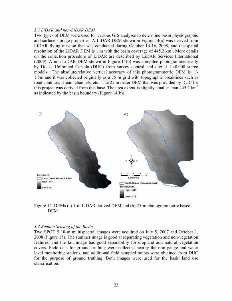
3.3 LiDAR and non-LiDAR DEM Two types of DEM were used for various GIS analyses to determine basin physiographic and surface storage properties. A LiDAR DEM shown in Figure 14(a) was derived from LiDAR flying mission that was conducted during October 14-16, 2008, and the spatial resolution of the LiDAR DEM is 1 m with the basin coverage of 445.2 km2. More details on the collection procedure of LiDAR are described by LiDAR Services International (2009). A non-LiDAR DEM shown in Figure 14(b) was compiled photogrammetrically by Ducks Unlimited Canada (DUC) from survey control and digital 1:40,000 stereo models. The absolute/relative vertical accuracy of this photogrammetric DEM is +/- 1.5m and it was collected originally as a 75 m grid with topographic breaklines such as road contours, stream channels, etc. The 25 m raster DEM that was provided by DUC for this project was derived from this base. The area extent is slightly smaller than 445.2 km2 as indicated by the basin boundary (Figure 14(b)).
(a) (b)
Figure 14. DEMs (a) 1-m LiDAR derived DEM and (b) 25-m photogrammetric based
DEM. 3.4 Remote Sensing of the Basin Two SPOT 5 10-m multispectral images were acquired on July 5, 2007 and October 1, 2008 (Figure 15). The summer image is good at separating vegetation and non-vegetation features, and the fall image has good separability for cropland and natural vegetation covers. Field data for ground truthing were collected nearby the rain gauge and water level monitoring stations, and additional field sampled points were obtained from DUC for the purpose of ground truthing. Both images were used for the basin land use classification.

24
Figure 15. SPOT 5 10-m multispectral images. (a) 2007 summer image and (b) 2008 fall
image.

25
4. Prairie Hydrological Model 4.1 Model Description The Cold Regions Hydrological Model platform (CRHM) was used to develop the Prairie Hydrological Model (PHM). CRHM is a “state-of-the-art” physically-based hydrological model and is based on a modular, object-oriented structure in which component modules represent basin descriptions, observations, or physically-based algorithms for calculating hydrological processes. The component modules have been developed based on the results of over 40 years of research by the University of Saskatchewan and National Water Research Institute in prairie, boreal, mountain and arctic environments. A full description of CRHM is provided by Pomeroy et al. (2007b). CRHM permits the assembly of a purpose-built model from a library of processes, and interfaces the model to the basin based on a user selected spatial resolution. The hydrological processes are simulated on landscape units called hydrological response units (HRU). HRUs are defined as spatial units of mass and energy balance calculation corresponding to hydrobiophysical landscape units, within which processes and states are represented by single sets of parameters, state variables, and fluxes. HRUs can be finely scaled (hillslope segment), or coarsely scaled (sub-basin). HRUs in the prairies typically correspond to agricultural fields (stubble or fallow fields), natural cover (grassland or forest woodland), and bodies of water (lake or pond) (Fang and Pomeroy, 2008). CRHM has shown good simulations in a semi-arid, well-drained prairie basin (Fang and Pomeroy, 2007) and in a sub-humid, poorly and internally drained prairie basin (Fang and Pomeroy, 2008). A set of physically based modules was linked in a sequential fashion to simulate the hydrological processes for the Smith Creek Research Basin. Figure 16 shows the schematic of these modules, and these modules include: 1. observation module: reads the meteorological data (temperature, wind speed, relative humidity, vapour pressure, precipitation, and radiation), providing these inputs to other modules; 2. interception module: divides precipitation between rainfall and snowfall depending on air temperature, and apportions precipitation to canopy modules (if used) or directly to the soil surface or snowpack.3 3. Garnier and Ohmura’s radiation module (Garnier and Ohmura, 1970): calculates the theoretical global radiation, direct and diffuse solar radiation, as well as maximum sunshine hours based on latitude, elevation, ground slope, and azimuth, providing radiation inputs to sunshine hour module, energy-budget snowmelt module, net all-wave radiation module; 4. sunshine hour module: estimates sunshine hours from incoming short-wave radiation and maximum sunshine hours, generating inputs to energy-budget snowmelt module, net all-wave radiation module; 5. Gray and Landine’s albedo module (Gray and Landine, 1987): estimates snow albedo throughout the winter and into the melt period and also indicates the beginning of melt for the energy-budget snowmelt module;

26
Garnier and Ohmura’s radiation module
Observationmodule
Sunshine hourmodule
Interception module
PBSM
Gray and Landine’s
Albedo module
EBSM
All-wave radiation module
Gray’s snowmelt infiltration module, Green-Ampt infiltration
Granger’s evaporation module, Priestley and Taylor
evaporation module
Soil moisture balance calculation with
wetland/depression storage and fill-and-spill module
Muskingum routing module
Global radiation
Max. sunshine
Temperature, WindspeedRelative HumidityVapour PressurePrecipitation
Sunshine hour
Rainfall Snowfall
SWE
albedo
snowmeltShort- and long-wave radiation Snow INF
Rain INF runoff
evapSoil moisture in recharge and rooting zones
Walmsley’s windflow module
Adjusted windspeed
Long-wavemodule
Canopy effect adjustment for
radiation module
Adjusted short- andlong-wave radiation
Figure 16. Flowchart of physically based hydrological modules for PHM. 6. longwave radiation module: estimates incoming longwave radiation for canopy energy balance estimation under clear or cloudy skies, using the modification of Brutsaert’s clear-sky longwave formulation by Sicart et al. (2006). 7. PBSM module or Prairie Blowing Snow Model (Pomeroy and Li, 2000): simulates the wind redistribution of snow and estimates snow accumulation throughout the winter period; 8. Walmsley’s windflow module (Walmsley et al., 1989): adjusts the wind speed change due to local topographic features and provides the feedback of adjusted wind speed to the PBSM module; 9. EBSM module or Energy-Budget Snowmelt Model (Gray and Landine, 1988): estimates snowmelt by calculating the energy balance of radiation, sensible heat, latent heat, ground heat, advection from rainfall, and change in internal energy; 10. canopy adjustment for radiation module (Sicart et al., 2004): adjusts the net all-wave radiation energy where woodland imposes effects of tree canopy on amount of radiation energy for melting snowpack underneath; 11. all-wave radiation module: calculates net all-wave radiation from the short-wave radiation and provides inputs to the evaporation module; 12. infiltration module (two types): Gray’s snowmelt infiltration (Gray et al., 1985) estimates snowmelt infiltration into frozen soils, Green-Ampt infiltration and redistribution expression (Ogden and Saghafian, 1997) estimates rainfall infiltration into

27
unfrozen soils, both infiltration algorithms update moisture content in the soil column from soil moisture balance with wetland/depression component module; 13. evaporation module (two types): Granger’s evaporation expression (Granger and Gray, 1989) estimates actual evaporation from unsaturated surfaces, Priestley and Taylor evaporation expression (Priestley and Taylor, 1972) estimates evaporation from saturated surfaces or water body, both evaporation update moisture content in the soil column, and Priestley and Taylor evaporation also updates moisture content in the wetland or depression from soil moisture balance with wetland or depression component module; 14. Muskingum routing module – the Muskingum method is based on a variable discharge-storage relationship (Chow, 1964) and is used to route the runoff between HRUs in the RB. The routing storage constant is estimated from the averaged length of HRU to main channel and averaged flow velocity; the average flow velocity is calculated by Manning’s equation (Chow, 1959) based on averaged HRU length to main channel, average change in HRU elevation, overland flow depth and HRU roughness; 15. soil moisture balance calculation with wetland or depression storage and fill-and-spill module: this is a newly developed module, specifically for basins such as Smith Creek, with prominent wetland storage and drainage attributes. This new wetland module was developed by modifying a soil moisture balance model, which calculates soil moisture balance and drainage (Dornes et al., 2008). This model was modified from an original soil moisture balance routine developed by Leavesley et al., (1983). The changes are to make this algorithm more consistent with what is known about prairie water storage and drainage (Pomeroy et al., 2007a). Figure 17 shows a flowchart of the wetland module. The soil moisture balance model divides the soil column into two layers; the top layer is called the recharge zone. Inputs to the soil column layers are derived from infiltration from both snowmelt and rainfall. Evapotranspiration withdraws moisture from both soil column layers. Evaporation only occurs from the recharge zone, and water for transpiration is taken out of the entire soil column. Excess water from both soil column layers satisfies groundwater flow requirements before being discharged to subsurface flow (representing flow in macropores that occurs in cracking clay, very coarse soils and in organic soils). The movement of runoff, subsurface discharge and groundwater discharge between HRUs is calculated by a routing module. Two new components - depression and pond – were added to the soil moisture balance model to model wetland drainage. Depressional storage represents small scale (sub-HRU) transient water storage on the surface of fields, pastures and woodlands. Pond storage represents water storage that dominates a HRU in wet conditions, though the pond can be permitted to dry up in drought conditions. The inputs to depressional storage are from surface runoff and overland flow after the soil column is saturated. After the depressional storage is filled, overland flow is generated via the fill-and-spill process, in which over-topping of the depression results in runoff but minimal leakage of water from the depression to sub-surface storage is permitted before it overtops. Evaporation is permitted from depressional storage. Pond storage works in a similar manner to depressional storage, except that the pond area does not have a soil column, and inputs are derived from uphill surface runoff and infiltration. In the wetland module, both depressions and ponds have storage capacity; the difference is that depressional storage represents ephemeral wetlands or drained wetlands on cultivated fields, whilst pond storage characterizes a large permanent or non-drained wetland or lake.

28
Ifpond
Snowmelt Rainfall
Snowmelt Infiltration
Rainfall Infiltration
Recharge Zone
Soil Column
Evapotranspiration
SubsurfaceDischarge
Groundwater GroundwaterDischarge
Ifsoil column
is full
Yes
No
No Yes
Saturated OverlandFlow = 0
SaturatedOverland
Flow
Ifdepression
NoRunoff
YesRunoff to
Depression
Depression
Evaporation
GroundwaterGroundwaterDischarge
SubsurfaceDischarge
Ifdepression
is full
NoNo fill-and-spill
Yesfill-and-spill
Snowmelt Rainfall
Snowmelt Infiltration
Rainfall Infiltration
Wetland Pond
Evaporation
Groundwater
Ifpond is full
No fill-and-spill
No
Yesfill-and-spill
SubsurfaceDischarge
GroundwaterDischarge
Surface Runoff
Figure 17. Flowchart of a wetland module of soil moisture balance calculation with wetland or depression storage and fill-and-spill.
29
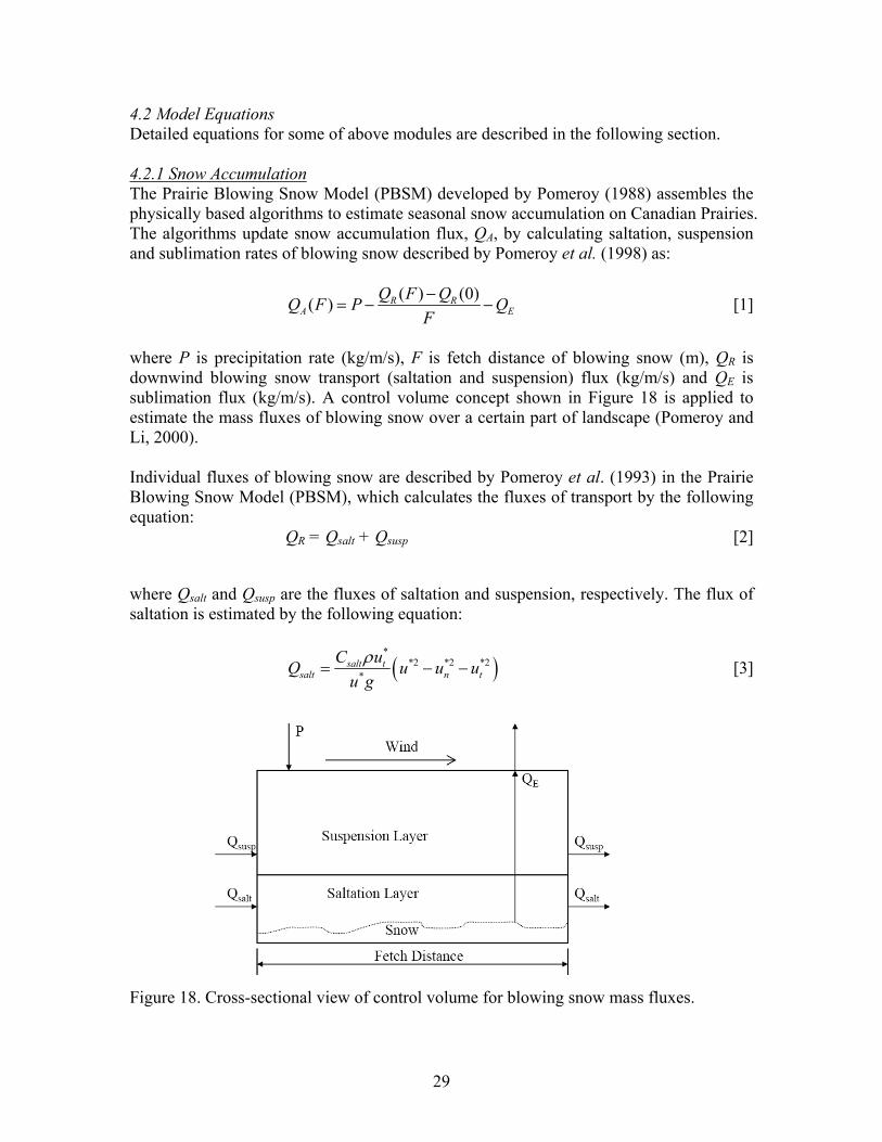
4.2 Model Equations Detailed equations for some of above modules are described in the following section. 4.2.1 Snow Accumulation The Prairie Blowing Snow Model (PBSM) developed by Pomeroy (1988) assembles the physically based algorithms to estimate seasonal snow accumulation on Canadian Prairies. The algorithms update snow accumulation flux, QA, by calculating saltation, suspension and sublimation rates of blowing snow described by Pomeroy et al. (1998) as:
( ) (0)( ) R R
A EQ F QQ F P Q
F−
= − − [1]
where P is precipitation rate (kg/m/s), F is fetch distance of blowing snow (m), QR is downwind blowing snow transport (saltation and suspension) flux (kg/m/s) and QE is sublimation flux (kg/m/s). A control volume concept shown in Figure 18 is applied to estimate the mass fluxes of blowing snow over a certain part of landscape (Pomeroy and Li, 2000). Individual fluxes of blowing snow are described by Pomeroy et al. (1993) in the Prairie Blowing Snow Model (PBSM), which calculates the fluxes of transport by the following equation:
QR = Qsalt + Qsusp [2]
where Qsalt and Qsusp are the fluxes of saltation and suspension, respectively. The flux of saltation is estimated by the following equation:
( )*
*2 *2 *2*
salt tsalt n t
C uQ u u uu gρ
= − − [3]
Figure 18. Cross-sectional view of control volume for blowing snow mass fluxes.

30
Where: Qsalt = saltation transport rate (kg/m/s), Csalt = empirical constant (0.68 m/s), ρ = atmospheric density (kg/m3), g = gravitational acceleration (m/s2), u* = atmospheric friction velocity (m/s), un
* = friction velocity applied to non-erodible surface elements (m/s), and ut
* = friction velocity applied to the snow surface (m/s). Equation [3] was formulated by Pomeroy and Gray (1990) to apply Bagnold’s framework (1954) for calculating the transport rate of saltating sand to saltating snow. Equation [3] includes the total atmospheric shear stress, τ, shear stress applied to non-erodible surface elements, τn, and shear stress applied to erodible surface elements, τt, to estimate the mean weight of saltating snow. The various types of shear stress are related to the corresponding friction velocity – u*, un
*, and ut*. The friction velocity is calculated as a
function of the wind profile:
*
0
ln[ ]zu ku zz
= [4]
where: uz = wind speed at height of z (m/s), k = von Kármán’s constant (0.4), z0 = aerodynamic roughness height (m). The non-erodible friction velocity, un
*, was found to equal zero for complete snow covers without exposed vegetation; the threshold friction velocity, ut
*, is the friction velocity at which transport ceases and was found in the range of 0.07-0.25 m s-1 for fresh, loose snow and higher range of 0.25-1.0 m s-1 for old, dense snow (Pomeroy and Gray, 1990). The flux of suspension is estimated by the following equation:
*
*
0
( ) ln( )bz
susph
u zQ z dzk z
η= ∫ [5]
where: Qsusp = suspension transport rate (kg/m/s), u* = atmospheric friction velocity (m/s), k = von Kármán’s constant, zb = upper boundary of suspension (m), h* = lower boundary of suspension (m), η(z) = mass concentration of suspended snow (kg/m3) at height z, and z0 = aerodynamic roughness height (m).

31
Pomeroy and Gray (1990), fitting wind speed measurements, found an expression for the aerodynamic roughness height over complete snow covers as a function of friction velocity, u*:
2*
0 0.12032uz
g= [6]
The lower boundary of suspension, h*, which defines the saltation-suspension interface was found to relate to friction velocity, u*:
1.27* *0.08436h u= [7] Pomeroy and Male (1992) developed an expression relating the mass concentration of suspended snow to height, z, and friction velocity, u*: * 0.544 0.544( ) 0.8exp[ 1.55(4.784 )]z u zη − −= − − [8] PBSM models the sublimation rate based on the energy equilibrium of radiation, convection of snow particles, water vaporation from snow particles, and sublimation (Schmidt, 1991). The sublimation rate is approximated by the following equation:
2 - -1
1-1
sr
T
s s
T s
L MQrTNu RTdm
L L MdtTNu RT D Sh
π σλ
λ ρ
⎛ ⎞⎜ ⎟⎝ ⎠=
⎛ ⎞ +⎜ ⎟⎝ ⎠
[9]
where: r = radius of a snow particle possessing mass m, σ = ambient atmospheric undersaturation of water vapour with respect to ice, Qr = radiative energy absorbed by the particle, Ls = latent heat of sublimation (2.838 × 10⁶ J kg-1), M = molecular weight of water (18.01 kg mol-1), λT = thermal conductivity of the atmosphere (λT = 0.00063T + 0.0673), Nu = Nusselt number, R = universal gas constant (8313 J mol-1 K-1), T = ambient atmospheric temperature, ρs = saturation density of water vapour at T, D = diffusivity of water vapour, and Sh = Sherwood number. A relation between the threshold friction velocity, ut
*, and air temperature (°C), T at 2-m height was derived by Li and Pomeroy (1997a):

32
2
* 0.35150 8200tT Tu = + + [10]
The Equation [10] provides a direct method to calculate threshold condition for blowing transport from meteorological data. Li and Pomeroy (1997b) found that the probability of blowing snow occurrence to follow a cumulative normal distribution with regard to the mean wind speed, umean, and the standard deviation δ of wind speed, u, as:
2
2( )
2
0
1 exp2
meanu uu
p duδ
δ π
−−
= ∫ [11]
They found the mean wind speed and the standard deviation of wind speed were as functions of snow conditions and air temperature based on extensive study on the Canadian prairies. For wet snow, the values of 21 and 7 m s-1 were found for the mean and standard deviation of wind speed, respectively. For dry snow packs, the mean and variance of wind speed were associated to air temperature (°C), T, and snow age index, I, as follows: 20.365 0.00706 0.9 11.2meanu T T I= + + + [12] 20.145 0.00196 4.3T Tδ = + + [13] Equation [11] allows the application of blowing snow fluxes calculation from the meteorological data and provides a technique for approximating areal blowing snow fluxes from a point. The estimation of snow mass balance using this technique was conducted in the Canadian arctic and prairie regions (Pomeroy and Li, 2000). 4.2.2 Snowmelt Snowmelt involves phase changes and hence the energy equation is traditionally taken as the physical framework for snowmelt estimations (Granger et al., 1977; Gray and Landine, 1988). The energy equation is based upon the law of conservation of energy to a control volume of snow, and this volume has a snow-ground interface and a snow-air interface as its lower and upper boundaries, respectively (Figure 19). The energy budget for calculating snowmelt involves energy and mass fluxes in radiation, convection, conduction, and advection along with a change in internal energy. The equation for the energy budget is expressed as:
Qm = Qn + Qh + Qe + Qg + Qp + QA – ∆U/∆t [14] where: Qm = energy flux available for snowmelt (W m-2), Qn = net radiation flux (W m-2), Qh = convective flux of sensible heat (W m-2), Qe = convective flux of latent heat (W m-2), Qg = conductive flux of ground flux (W m-2),

33
Qp = advection from rain in vertical direction (W m-2), QA = small-scale advection from patches of soils in horizontal direction (W m-2),
∆U/∆t = rate of change in internal energy (W m-2).
Figure 19. Cross-sectional view of control volume for snowmelt energies. Individual terms in the energy budget equation can be determined by existing equations. Net radiation, Qn, is the total of the net short-wave, Qsn, and net long-wave, Qln, expressed as: Qn = Qsn + Qln [15] where the net-long wave is normally negative and the energy fluxes directed towards the snow pack are considered as positive. The net-short wave is the sum of the incident short-wave flux, Qs, received by the surface and reflected short-wave flux, Qr, by the surface; the reflectance short-wave energy is a fraction of the incident short-wave, which is expressed as the albedo of snow, αs, normally in the range of 0.65-0.95 depending on the age of snow. Thus, the net-short wave is expressed as: Qsn = Qs(1 – αs) [16] The incident short-wave flux, Qs, is total of its direct beam, Qdrs, and diffuse, Qdfs components, expressed as: Qs = Qdrs + Qdfs [17] With cloud cover, the amount of direct beam short-wave flux is reduced and found to be a function of the direct beam short-wave radiation under clear sky, Qdro, as:
[ ( ) ]cdrs dro
nQ Q a bN
= + [18]

34
where n/N is the sunshine ratio; a, b, and c are coefficients and are found to equal 0.024, 0.974, and 1.35, respectively, for the southwestern prairie region of Saskatchewan (Granger and Gray, 1990). The direct beam short-wave radiation under clear sky, Qdro, is estimated by the expression developed by Garnier and Ohmura (1970). The atmospheric constituents (e.g. dust particles, water droplets, and ice crystals) reduce the transmissivity for beam radiation and increase the scattering and diffusion. Granger and Gray (1990) derived a relation for estimating the diffuse flux with cloud cover, Qdfs, as a function of diffuse radiation under clear sky, Qdfo, and the sunshine ratio, n/N, as:
2[2.68 2.2( ) 3.85( ) ]dfs dfon nQ QN N
= + − [19]
The clear-sky diffuse radiation, Qdfo, can be the expression derived by Granger and Gray (1990) that relates Qdfo to the atmospheric pressure ratio, cosine of the angle of incidence of the sun’s rays on a slope, and day of year. The net-long wave flux, Qln, is the sum of the downward radiation emitted by the atmosphere, Ql↓, and the upward radiation emitted by the surface, Ql↑. Due to the influence of diurnal changing temperature on the internal energy content of shallow snowcovers, it is important to incorporate the long-wave into the snowmelt estimation. Granger and Gray (1990) developed an expression for calculating the net long-wave flux under cloud cover, Qln, for the southwestern prairie region of Saskatchewan as:
ln ln [0.25 0.75( )]onQ QN
= + [20]
where n/N is the sunshine ratio; Qlno is the clear sky net long-wave radiation, estimated by the following expression relating to the clear sky short-wave radiation, Qso: ln 4.25 0.24o soQ Q= − − [21]
Male and Gray (1981) outlined simplified bulk transfer expressions for calculating convective sensible heat flux Qh and latent heat flux Qe:
Qh = DhUz(Ta – Ts) and [22] Qe = DeUz(es – ea) [23] where: Dh = bulk transfer coefficient for sensible heat transfer (kJ/m3·°C), De = bulk transfer coefficient for latent heat transfer (kJ/m3·°C), Uz = wind speed at a reference height (m/s), Ta, Ts = temperature of the air and the snow surface, respectively (°C), es, ea = vapour pressures of the air and snow surface, respectively (mb). Internal energy U is estimated by the following equations (Male and Gray, 1981):
U = d(ρiCPi +ρlCPl +ρvCPv)Tm [24]

35
where: d = depth of snow (m), ρ = density (Kg/m3), CP = specific heat (KJ/kg·°C), Tm = mean snow temperature (°C), and i, l, v = ice, liquid and vapor phases, respectively.
When rain falls on a melting snow pack where the rain does not freeze, the advection flux from rain is estimated by the following equation (Male and Gray, 1981):
Qp = 4.2(Tr – Ts)Pr [25] where: Tr = temperature of the rain (°C), Ts = snow temperature (°C), and Pr = depth of rain (mm/day). The amount of melt can be calculated from Qm by the equation:
m
w f
QMBhρ
= [26]
where: ρw = density of water (1000 kg m-3), B = fraction of ice in a unit of wet snow (0.95 → 0.97), hf = latent heat of fusion of ice (333.5 kJ kg-1). 4.2.3 Infiltration i. Snowmelt Infiltration On Canadian Prairies Granger et al. (1984) developed an empirical equation for estimating cumulative infiltration (INF) of limited infiltrability frozen soils based on the SWE and average pre-melt water and ice content of 0-300 mm soil layer (SI). Gray et al. (1985) successfully derived its expression as:
0.5845 (1 )IINF S SWE= ⋅ − ⋅ [27]
Zhao et al. (1997) developed a physically-based finite difference numerical model, HAWTS (Heat And Water Transport in frozen Soils). The model estimates moisture movement related to sensible and latent heat transfers in frozen soils based on a set of partial differential equations. Zhao and Gray (1999) developed a parametric form of the HAWTS model that describes cumulative infiltration into frozen unsaturated soils of limited infiltrability as:
0.452.92 1.64 0.440 0
273.15(1 )273.15
II
TINF C S S t−−⎛ ⎞= ⋅ ⋅ − ⋅ ⋅⎜ ⎟
⎝ ⎠ [28]

36
where C is a constant and is found to be 2.10 and 1.14 for the prairie soils and forest soils, respectively (Gray et al., 2001). S0 is the surface saturation (mm3 mm-3) and is assumed to be between 0.75 and 1.00, and approximately equal to 1 in most situations when infiltration rate is low and snowmelt is rapid (Gray et al., 2001). SI is the average soil saturation of top 40 cm soil layer at the start of infiltration (mm3 mm-3) and is estimated from the average pre-melt volumetric moisture content (water + ice) (θI) divided by the soil porosity (Φ). θI can be approximated from the fall soil moisture θf based on empirical expressions developed on Canadian agricultural region (Gray et al., 1985) as:
5.08 1.05I fθ θ= − + (for fallow fields) [29] 0.294 0.957I fθ θ= + (for stubble fields) [30]
TI is the average initial temperature of top 40 cm of soil (K). t0 is the infiltration opportunity time (h) and approximately equals the time required to melt the snow cover and is estimated by the following equation:
0SWEt tMelt
≅ = [31]
The assumptions made for the parametric equation are that soil is homogeneous and isotropic, distributions of initial soil temperature and moisture are uniform, and meltwater has a constant head at the soil surface (Zhao and Gray, 1999). ii. Rainfall Infiltration The rainfall infiltration rate according to the original Green and Ampt (1911) equation for a single ponding event is
1θ θψ −⎛ ⎞= − +⎜ ⎟⎝ ⎠
s ip s ff K
F [32]
where: fp = potential infiltration rate (cm/s), Ks = soil saturated hydraulic conductivity (cm/s), ψf = suction at wetting front (negative pressure head), θi = initial moisture content (dimensionless),
θs = saturated moisture content (dimensionless) and F = cumulative infiltration (cm). Rearranging gives the cumulative infiltration F as a function of infiltration rate fp
1
θ θψ −= −
+
s if
p
s
F fK
[33]

37
4.2.4 Evaporation Actual evaporation from natural non-saturated surfaces is estimated according to the evaporation expression of Granger and Gray (1989)
( )( ) ( )
γγ γ
∗Δ −= +
Δ + Δ +c g A
Gk Q Q GEEG G
[34]
where: Q* = net radiation (W m-2), Qg = ground heat flux (W m-2), Kc = unit conversion coefficient to provide evaporate in mm/day, ∆ = slope of the saturation vapour pressure curve (kPa/○C), γ = psychrometric constant (kPa ○C-1),
G = relative evaporation, EA = drying power (mm/day).
Details for each term above are discussed by Granger and Gray (1989; 1990). Potential evaporation over horizontally uniform saturated surfaces is estimated by the expression of Priestley and Taylor (1972)
( )*gPE Q Qα
γΔ
= −Δ + [35]
where: Q* = net radiation (W m-2), Qg = ground heat flux (W m-2), ∆ = slope of the saturation vapour pressure curve (kPa/○C), γ = psychrometric constant (kPa ○C-1),
α = dimensionless empirical correction coefficient (1.26).

38
5. Modelling Parameterization Methods A pre-processing procedure was taken to estimate the values for the parameters in CRHM. The procedure was essentially a model parameterization based on field observations, lookup table values, and analysis of remote sensing and GIS. Two types of modelling approaches: non-LiDAR calibrated and LiDAR-based uncalibrated were involved. The calibrated modelling used a coarse photogrammetric based DEM as input, while the uncalibrated modelling utilized the LiDAR derived DEM in the analysis. They have the same methods for deriving all parameter values except for surface depression storage. In the calibrated modelling, surface depression storage in the upland area was calibrated and surface depression storage in the wetland area was estimated by an area-volume regression equation, while uncalibrated modelling used an automated procedure with a depth-area-volume relationship (Hayashi and van der Kamp, 2000; Minke et al., in review). The basin area with the uncalibrated modelling based on LiDAR was likely more accurate than the coarse scale basin area used in the calibrated model. The details on estimating the model parameters are described in the following sections. 5.1 Determination and Estimation of Parameters 5.1.1 Sub-basin and HRU Determination For modelling large basins such as Smith Creek Research Basin (SCRB), CRHM has a new component feature called “representative basins” (RB), in which a set of physically based modules are assembled with a certain arrangement of HRUs to represent a sub-basin. Streamflow output from a number of RBs are then routed along the main stream through lakes, wetlands and channel. Both calibrated and uncalibrated approaches divided the SCRB into five sub-basins, which are represented by five RBs (Figure 20). Figure 21 shows the procedure used by calibrated and uncalibrated approaches for extracting sub-basins. Both modelling approaches employed same automated basin delineation technique “TOPAZ” (Garbrecht and Martz, 1993; 1997), while a 25-m photogrammetric based DEM and a 1-m LiDAR DEM were used for the calibrated and uncalibrated approaches, respectively. Both DEM inputs were resampled to 50-m for a computational efficiency reason. The calibrated approach failed to delineate the TOPAZ channel and sub-basin segments due to the poor quality of the photogrammetric based DEM, and the five sub-basins were manually defined by examining the Ducks Unlimited Canada (DUC) aerial photography and satellite imagery, and drainage networks GIS data. The uncalibrated approach was able to generate TOPAZ channel and sub-basin segments, which were aggregated to five sub-basins. Within each RB, seven hydrological responses units (HRUs) were derived from a supervised land use classification based on two SPOT 5 10-m multispectral images that were acquired on 5 July 2007 and 1 October 2008. Figure 22 illustrates the process involving the generation of HRUs for the SCRB. Fallow, stubble, grassland/pasture, wetland (shrubs), open water, woodland, and town/road were produced from the supervised classification. A post-classification accuracy analysis was conducted using ground truthing points acquired from field surveys and DUC land use segmentation,

39
66.7% of overall accuracy was achieved. In addition, Smith Creek drainage network GIS data (2000) was used to extract the river channel. For both modelling approaches, fallow, stubble, grassland, wetland, open water, woodland, and river channel HRUs were aggregated from the supervised classification and DUC drainage network data.
RB 1•Fallow HRU•Stubble HRU•Grassland HRU•River Channel HRU•Open Water HRU•Woodland HRU•Wetland HRU
Physically-based hydrological modules
RB 2•Same seven HRUs
Sub-basin 1
Sub-basin 2
Sub-basin 3
Sub-basin 4
Sub-basin 5
Muskingumrouting betweensub-basins
RB 3•Same seven HRUs
RB 4•Same seven HRUs
RB 5•Same seven HRUs
Figure 20. CRHM modelling structure. Five Sub-basins are simulated by modelling
structure “Representative Basin” (RB); same seven hydrological response units (HRUs) exist in each RB. Modelling structure of Muskingum routing connects all five RBs.
5.1.2 Basin Physiographic Parameters Both modelling approaches used a number of parameters for basin physical characteristics for the seven HRUs, including HRU area, HRU elevation, latitude, and ground slope (Table 2). HRU area was determined from SPOT 5 land use classification and DUC drainage networks GIS data. The average elevation for HRU at different sub-basins was determined from the DEM and HRU classification. The latitude (geographic centre of SCRB) was measured from a GPS. The average ground slope was approximated from the reported slope values in Saskatchewan Soil Survey (1991) for use in correcting incoming solar radiation. As these corrections were small in this flat landscape, the soil survey slopes were sufficiently accurate. 5.1.3 Albedo and Canopy Parameters For both modelling approaches a list of albedo parameters for bare ground and snow, as well as the canopy parameter LAI (leaf area index) was developed for the HRUs. The values of these parameters are shown in Table 3. The albedo parameters 0.17 and 0.85 were determined for bare ground and snow respectively, based on recommended values by Male and Gray (1981). The canopy parameter, LAI, was used to model canopy effects on radiation for snowmelt. Small values of LAI (0.001) were set for fallow, stubble,

40
grassland, river channel, open water and wetland HRUs, 0.4 was assigned to woodland HRUs, representing a typical LAI value for aspen trees during the winter at SCRB.
Manualsub-basindelineation
Sub-basinaggregationfrom TOPAZsub-basinsegments
Calibrated Approach Uncalibrated Approach
(a)
(f)(e)
(c) (d)
(b)
TOPAZautomateddelineation
TOPAZautomateddelineation
Figure 21. Pre-processing procedure for deriving sub-basins at Smith Creek Research
Basin. (a) 50-m resampled photogrammetric based DEM, (b) 50-m resampled LiDAR DEM, (c) TOPAZ channel and sub-basin segments from the calibrated non-LiDAR approach, (d) TOPAZ channel and sub-basin segments from the Uncalibrated LiDAR approach, (e) sub-basins from the calibrated non-LiDAR approach, and (f) sub-basins from the uncalibrated LiDAR approach.

41
(a) (b)
(e)(d)(c)
Supervised landuse classification
Generation of seven HRUs
Figure 22. Pre-processing procedure for generating HRU classification at Smith Creek
Research Basin. (a) 2007 summer SPOT 5 10-m multispectral image, (b) 2008 fall SPOT 5 10-m multispectral image, (c) supervised land use classification for the basin derived from the calibrated non-LiDAR approach, (d) supervised land use classification for the basin derived from the uncalibrated LiDAR approach, and (e) Ducks Unlimited Canada drainage networks in 2000.

42
Table 2. Basin physiographic parameters. HRU area values shown inside parentheses are derived from the uncalibrated LiDAR approach and the values outside parentheses are extracted from the calibrated non-LiDAR approach.
HRU Area (km2) HRU Elevation (m)
HRU Name Sub-
basin 1 Sub-
basin 2 Sub-
basin 3 Sub-
basin 4 Sub-
basin 5 Sub-
basin 1 Sub-
basin 2 Sub-
basin 3 Sub-
basin 4 Sub-
basin 5 Latitude
(º) Ground Slope (º)
Fallow 5.1
(6.3) 3.3
(1.7) 2.3
(2.1) 4.1
(3.1) 0.6
(0.3) 530 528 526 520 510 51.1 4
Stubble 81.2
(121.9) 61.1
(31.0) 54.7
(34.5) 34.2
(21.8) 10.7 (6.3) 528 526 524 514 505 51.1 4
Grassland 19.2
(22.6) 6.5
(2.7) 7.3
(5.5) 2.4
(1.4) 1.1
(0.7) 528 526 524 514 505 51.1 4 River Channel
0.6 (0.8)
0.3 (0.2)
0.6 (0.5)
0.4 (0.2)
0.1 (0.1) 526 520 512 510 500 51.1 4
Open Water 9.1
(10.5) 3.3
(0.9) 0.7
(0.5) 0.5
(0.4) 0.1
(0.1) 527 522 518 512 502 51.1 0
Woodland 41.4
(49.0) 27.0
(12.4) 16.0
(12.7) 12.4 (9.2)
5.1 (3.1) 527 522 518 512 502 51.1 0
Wetland 16.9
(23.2) 9.7
(2.6) 3.6
(2.7) 2.5
(1.8) 1.0
(0.5) 527 522 518 512 502 51.1 0 Table 3. Albedo and canopy parameters.
HRU Name Bare Ground Albedo Snow Albedo LAI Fallow 0.17 0.85 0.001 Stubble 0.17 0.85 0.001 Grassland 0.17 0.85 0.001 River Channel 0.17 0.85 0.001 Open Water 0.17 0.85 0.001 Woodland 0.17 0.85 0.4 Wetland 0.17 0.85 0.001

43
5.1.4 Blowing Snow and Frozen Soil Parameters Both calibrated and uncalibrated modelling used the same method for estimating blowing snow and frozen soil parameters shown in Table 4. Blowing snow fetch distance is the upwind distance without disruption to the flow of snow. A computer program “FetchR” (Lapen and Martz, 1993) was used to estimate the fetch for the large exposed areas fallow, stubble and grassland HRUs from the DEM and vegetation classification, resulting in fetches of 1000 m, 1000 m, and 500 m respectively. For river channel, open water, woodland and wetland HRUs, a 300 m fetch length was assigned. The vegetation height, stalk density and stalk diameter were calculated based on vegetation survey measurements. The distribution factor parameterizes the allocation of blowing snow transport from aerodynamically smoother (or windier) HRU to aerodynamically rougher (or calmer) ones and was decided according to the prairie landscape aerodynamic sequencing (Fang and Pomeroy, 2009). Lower values indicate lower aerodynamic roughness (or higher wind speed) and higher value means greater roughness (or lower wind speed). The values presented in Table 4 allow snow to be transported from fallow and open water to stubble HRUs and then to grassland and woodland HRUs, and subsequently to river channel and wetland HRUs according to what was observed in the field. A frozen soil infiltration parameter reflecting fall soil saturation was determined from the soil porosity and observed fall soil moisture. The soil porosity was estimated from soil texture, which is predominately loam in the basin. Fall soil moisture was approximated from gravimetric measurement of soil survey samples. Table 4 shows values of 100% for river channel and open water HRUs, indicating that both are saturated. Table 4. Blowing snow and frozen soil parameters. Initial fall soil saturation values inside parentheses are for the fall of 2008 and values outside parentheses are for the fall of 2007.
HRU Name Fetch (m)
Vegetation Height (m)
Stalk Density (#/m2)
Stalk Diameter (m)
Distribution Factor
Initial Fall Soil Saturation (%)
Fallow 1000 0.001 320 0.003 0.1 46 (55) Stubble 1000 0.12 320 0.003 0.5 50 (58) Grassland 500 0.4 320 0.003 1 54 (65) River Channel 300 0.7 1 0 2 100 (100) Open Water 300 0.001 1 0 0.5 100 (100) Woodland 300 6 100 0.01 1 53 (49) Wetland 300 1.5 100 0.01 3 87 (91) 5.1.5 Routing Parameters Both modelling approaches used the same method to determine routing parameters. Parameters for routing surface runoff between HRUs within sub-basins (RBs) are shown in Tables 5 and 6, and parameters for routing channel flow between five RBs are shown in Table 7. These parameters were used in the Muskingum routing module (Chow, 1964). For the routing within RBs, the routing length is the distance from each HRU to the main channel; for the routing between RBs, the routing length is the main channel length in each sub-basin, and both types of routing length were estimated from DUC drainage networks GIS data. Manning’s equation (Chow, 1959) was used to calculate the average flow velocity; the parameters used in the equation include hydraulic radius, longitudinal friction slope, and Manning’s roughness coefficient. Hydraulic radius was determined

44
Table 5. Parameters for runoff routing between HRUs within the sub-basins (RBs). Routing Length to Stream (m)
HRU Name
Sub-basin
1
Sub-basin
2
Sub-basin
3
Sub-basin
4
Sub-basin
5 Manning's Roughness
Hydraulic Radius
(m)
Longitudinal friction
Slope (º)
Dimensionless Weighting
Factor Fallow 6000 5000 5000 4000 2000 0.04 0.01 0.001 0.25 Stubble 6000 5000 5000 4000 2000 0.05 0.01 0.001 0.25 Grassland 6000 5000 5000 4000 2000 0.11 0.01 0.001 0.25 River Channel 6000 5000 5000 4000 2000 0.035 0.01 0.001 0.25 Open Water 6000 5000 5000 4000 2000 0.11 0.01 0.00002 0.25 Woodland 6000 5000 5000 4000 2000 0.2 0.01 0.00002 0.25 Wetland 6000 5000 5000 4000 2000 0.2 0.01 0.00002 0.25 Table 6. Routing distribution parameter between HRUs within the sub-basins (RBs).
HRU Name Fallow Stubble GrasslandRiver
Channel Open Water Woodland Wetland Fallow 0 0 0 0.28 0.13 0.38 0.21 Stubble 0 0 0 0.28 0.13 0.38 0.21 Grassland 0 0 0 0.28 0.13 0.38 0.21 Open Water 0 0 0 1 0 0 0 Woodland 0 0 0 0.45 0.21 0 0.34 Wetland 0 0 0 0 1 0 0 River Channel 0 0 0 0 0 0 0 Table 7. Parameters for channel routing between the sub-basins (RBs). The values of area
and routing length inside parentheses are derived from the uncalibrated modelling and the values outside parentheses are determined from calibrated modelling.
Sub-basin Area (km2)
Routing Length (m)
Manning's Roughness
Hydraulic Radius (m)
Longitudinal friction Slope (º)
Dimensionless Weighting Factor
1 173.5 (234.3) 8000 (15000) 0.035 1 0.002 0.25 2 111.1 (51.7) 10000 (10000) 0.035 0.67 0.002 0.25 3 85.2 (58.5) 20000 (13000) 0.035 1 0.004 0.25 4 56.6 (37.9) 8000 (8000) 0.035 0.67 0.002 0.25 5 18.7 (11.0) 7000 (7000) 0.035 1 0.001 0.25
from flow depth based on the channel shape. Longitudinal friction slope was calculated from the DEM and DUC drainage networks GIS data; the average change in elevation over a routing length was approximated. Manning’s roughness coefficient was estimated based on the channel’s condition. The storage constant was estimated from the average flow velocity and routing length. The dimensionless weighting factor controls the level of attenuation, ranging from 0 (maximum attenuation) to 0.5 (no attenuation), so 0.25 was used for the basin. The routing sequence is illustrated in Figure 23. For the routing within RBs, runoff generated in the upland fallow, stubble, and grassland HRUs is routed to the upland woodland HRU, and is then routed to wetland, open water, and river channel

45
HRUs. Runoff from the wetland HRU is accumulated in the open water HRU, which connects to the river channel HRU. The routing distribution parameter shown in Table 6 is used to partition amount of runoff between HRUs and the values were determined from a modified Hack’s law length-area relationship (Granger et al., 2002). For each non-river channel HRU, the land use polygons from the supervised classification shown in Figure 22 were used to extract total polygon area and the longest linear length within the polygon. The extracted area and longest length were graphed on a log-log plot to generate the modified Hack’s law length-area relationship: 0.55591.2815L A= (fallow HRU) [36]
0.53911.3486L A= (stubble HRU) [37] 0.54611.2965L A= (grassland HRU) [38] 0.5421.2947L A= (open water HRU) [39] 0.53561.3587L A= (woodland HRU) [40] 0.551.2588L A= (wetland HRU) [41]
where L (km) is Hack’s law length for each HRU and A (km2) is total area for each HRU. For the river channel HRU, the original Hack’s law length-are relationship (Hack, 1957) was used:
0.61.4L A= (river channel HRU) [42] where L (km) is Hack’s law length for river channel HRU and A (km2) is the average sub-basin area. The routing distribution parameter was calculated using the estimated Hack’s law length. For instance, the routing distribution parameters for runoff from fallow HRU to river channel, open water, woodland, and wetland HRUs are:
_ river channelfallow river channel
river channel open water woodland wetland
Ldistrib RouteL L L L→ =
+ + + [43]
_ open waterfallow open water
river channel open water woodland wetland
Ldistrib Route
L L L L→ =+ + +
[44]
_ woodlandfallow woodland
river channel open water woodland wetland
Ldistrib RouteL L L L→ =
+ + + [45]
_ wetlandfallow wetland
river channel open water woodland wetland
Ldistrib RouteL L L L→ =
+ + + [46]
The zero values in Table 6 indicate no routing for the non-river channel HRUs and imply outlet of each sub-basin (RB) for the river channel HRU. For the routing between RBs, runoff from each RB outlet flows to the main channel, which is connected in the sequence shown in Figure 23(b). This sequence was decided from the observed channel flow order in the field.

46
Fallow
River Channel
Open Water
Stubble Grassland
Woodland
WetlandRB outlet
RB 1
RB 2
RB 4
RB 3RB 5 Smith Creek
basin outlet
(a) (b) Figure 23. Routing sequence. (a) Between HRUs within the sub-basin (RB) and (b)
between RBs. 5.1.6 Wetland Module Parameters Table 8 shows parameters for soil recharge layer, soil column, subsurface and groundwater drainage. For the soil column, the maximum water holding capacity was determined from multiplying the rooting zone depth by soil porosity; the initial value of available water in the soil column was estimated by multiplying the maximum water holding capacity by volumetric soil moisture content. The soil recharge layer is the shallow top layer of the soil column, approximately 60 mm; the initial value of available water in the soil recharge layer was determined by multiplying the maximum water holding capacity and volumetric soil moisture content. It should be noted that the model treats river channel, open water, and wetland HRUs as having no soil column, but permanent surface ponding. Subsurface and groundwater drainage factors control the rate of flow in the subsurface and groundwater domains; these rates are slow in the prairie environment (Hayashi et al., 1998) and were estimated from the saturated hydraulic conductivity based on soil texture. Both modelling approaches used these same methods. Table 8. Parameters of soil recharge layer, soil column, and subsurface and groundwater
drainage for the wetland module. Initial values of available water in soil recharge layer and soil column inside parentheses are for the fall of 2008 and the values outside parentheses are for the fall of 2007.
Soil Recharge Layer Soil Column
HRU Name
Initial Value of Available
Water (mm)
Maximum Water Holding Capacity
(mm)
Initial Value of Available Water
(mm)
Maximum Water Holding Capacity
(mm)
Subsurface and Groundwater
Drainage Factor (mm day-1)
Fallow 28 (33) 60 276 (330) 600 0.001 Stubble 30 (35) 60 300 (348) 600 0.001 Grassland 32 (39) 60 324 (390) 600 0.001 River Channel 0 0 0 0 0.001 Open Water 0 0 0 0 0.001 Woodland 32 (29) 60 318 (294) 600 0.001 Wetland 0 0 0 0 0.001

47
Besides differences in basin area from the improved DEM derived from LiDAR, the major difference between the calibrated and uncalibrated modelling is the method used for estimating the surface depression capacity. Table 9 shows the parameters describing surface depression storage. For the calibrated modelling, the maximum surface depression storage in the wetland area (wetland and open water HRUs) was estimated from the average value of individual wetland storage as determined from a surface area- volume relation for prairie wetlands (Wiens, 2001). The relationship was slightly modified to derive values in the appropriate SI units required by the model
1.22
max
1000 2.8510000
A
sdA
⎡ ⎤⎛ ⎞⎢ ⎥⎜ ⎟
⎝ ⎠⎢ ⎥⎣ ⎦= [47]
max
1000 7.1 9.9710000
A
sdA
⎡ ⎤⎛ ⎞ +⎜ ⎟⎢ ⎥⎝ ⎠⎣ ⎦= [48]
where sdmax (mm) is the maximum surface depression storage, and A [m2] is the wetland surface area which was obtained from DUC wetland GIS inventory (2000). Equation [47] is for wetlands with surface area up to 700,000 m2, and Equation [48] is for wetlands with surface area greater than 700,000 m2. The calibrated non-LiDAR approach found the maximum surface depression storage in the upland area (fallow, stubble, grassland, and woodland HRUs) by comparing the simulated and observed hydrographs and optimising the storage value to match the hydrographs. For the uncalibrated LiDAR DEM based modelling, an automated procedure involving LiDAR DEM and various ArcGIS tools was used to extract initial depth, area and volume of surface depression which were in turn input into a depth-area-volume relationship, yielding final depth, area and volume of surface depression. The procedure is illustrated in Figure 24. The LiDAR DEM was resampled from its original 1-m spatial resolution to 10-m, and a “fill pits” was used to created a depressionless DEM from the 10-m LiDAR DEM; both were used as inputs to the ArcGIS 3D spatial analyst “cut/fill” feature. The “cut/fill” detects changes on area and volume of a surface between two periods due to addition or removal of material. If a surface is characterized as “cut” from erosion, it is categorized into ‘net loss’, and if a surface is identified as “fill” from deposition, then it is regarded as ‘net gain’, and ‘unchanged’ is another category if there is no change on the area and volume of a surface. Using both the original DEM and the depressionless DEM in the “cut/fill” created a virtual surface during two periods and generated only one category ‘net gain’, which comprises the Smith Creek basin “cut/fill” surface depressions shown in Figure 25. A comparison between the “cut/fill” depressions and DUC wetland inventory was made in the northern part of basin which is of great interest of farmers and various researchers (Figure 25(d)). It showed good agreement between these two approaches; even though the “cut/fill” output had more coverage, it is reasonable considering DUC wetland data was collected in 2000 during drought conditions. DUC sub-basin wetland GIS inventory and the basin “cut/fill” surface depressions were input in the ArcGIS “Intersect” tool, producing area and volume of sub-basin “cut/fill” surface

48
Table 9. Parameters of surface depression storage for the wetland module. The values inside parentheses are derived from the uncalibrated LiDAR DEM information and the values outside parentheses are determined from calibrated modelling.
Initial Value of Surface Depression Storage (mm) Maximum Surface Depression Storage Capacity (mm) HRU Name Sub-basin 1 Sub-basin 2 Sub-basin 3 Sub-basin 4 Sub-basin 5 Sub-basin 1 Sub-basin 2 Sub-basin 3 Sub-basin 4 Sub-basin 5 Fall of 2007 Fallow 0 (0) 0 (0) 0 (0) 0 (0) 0 (0) 70 (61) 70 (67) 70 (69) 70 (67) 70 (69) Stubble 0 (0) 0 (0) 0 (0) 0 (0) 0 (0) 70 (61) 70 (67) 70 (69) 70 (67) 70 (69) Grassland 0 (0) 0 (0) 0 (0) 0 (0) 0 (0) 70 (86) 70 (100) 70 (95) 70 (104) 70 (102) River Channel 54 (54) 54 (54) 54 (54) 54 (54) 54 (54) 200 (200) 200 (200) 200 (200) 200 (200) 200 (200) Open Water 59 (86) 56 (101) 56 (107) 54 (104) 52 (99) 221 (317) 208 (374) 208 (395) 202 (386) 195 (366) Woodland 0 (0) 0 (0) 0 (0) 0 (0) 0 (0) 140 (78) 140 (86) 140 (90) 140 (88) 140 (87) Wetland 59 (86) 56 (101) 56 (107) 54 (104) 52 (99) 221 (317) 208 (374) 208 (395) 202 (386) 195 (366) Fall of 2008 Fallow 0 (0) 0 (0) 0 (0) 0 (0) 0 (0) 70 (61) 70 (67) 70 (69) 70 (67) 70 (69) Stubble 0 (0) 0 (0) 0 (0) 0 (0) 0 (0) 70 (61) 70 (67) 70 (69) 70 (67) 70 (69) Grassland 0 (0) 0 (0) 0 (0) 0 (0) 0 (0) 70 (86) 70 (100) 70 (95) 70 (104) 70 (102) River Channel 76 (76) 76 (76) 76 (76) 76 (76) 76 (76) 200 (200) 200 (200) 200 (200) 200 (200) 200 (200) Open Water 84 (120) 79 (142) 79 (150) 77 (147) 74 (139) 221 (317) 208 (374) 208 (395) 202 (386) 195 (366) Woodland 0 (0) 0 (0) 0 (0) 0 (0) 0 (0) 140 (78) 140 (86) 140 (90) 140 (88) 140 (87) Wetland 84 (120) 79 (142) 79 (150) 77 (147) 74 (139) 221 (317) 208 (374) 208 (395) 202 (386) 195 (366)

49
LiDAR DEM (10 m) LiDAR depressionless DEM (10 m)“fill pits”
ArcGIS “3D cut/fill” tool
• Net Gain
• Unchanged
• Net Loss
• Net Gain (basin “3D cut/fill”surface depressions)
• Volume
•Area
DUC Smith Creek sub-basin wetland
GIS inventory
Smith Creek current sub-basin supervised landuse
classification
Estimated volume and area from “3D cut/fill” for Smith
Creek sub-basin wetland area
ArcGIS “Intersect” toolArcGIS “Intersect”tool
Estimated volume and area from “3D cut/fill” for each landuse at
Smith Creek sub-basin
ArcGIS “Erase” tool
Estimated volume and area from “3D cut/fill” for Smith
Creek sub-basin upland area
max maxmax 1 2 /
×=
+A dV
p
max 3 _ /= D cut fillA A
(3D cut/fill crude estimation for volume)3 _ / 3 _ / 3 _ /= ×D cut fill D cut fill D cut fillV d A
Maximum volume (m3) estimation from a simplified depth-area-volume method:
solve ‘d3D_cut/fill’ inversely
3 _ /3 _ /
3 _ /
= D cut fillD cut fill
D cut fill
Vd
Amax 3 _ / _ _= +D cut filld d fall depth adjustment
wetland area:
upland area:max 3 _ /= D cut filld d
shape coefficient: 1.723.36
===
ppp
if Amax < 10,000 m2
if 10,000 m2 <= Amax <= 100,000 m2
if Amax > 100,000 m2
Maximum surface depressionstorage sdmax (mm) in CRHM:
max maxmax
max
1000 10001 2 /
= × = ×+
V dsdA p
Figure 24. Flowchart of an automated procedure used by the uncalibrated modelling for
estimating maximum surface depression storage.

50
(d)
Figure 25. ArcGIS 3D “cut/fill” analysis. (a) Original Smith Creek basin 10-m LiDAR
DEM, (b) filled depression-less Smith Creek basin 10-m LiDAR DEM, (c) Smith Creek basin “cut/fill” surface depressions, the dark outline showing the northern part of Smith Creek Research Basin, and (d) comparison between “cut/fill” output (in red) and DUC 2000 wetland data (in black slash) in the northern part of Smith Creek Research Basin.

51
depressions in the wetland area. The sub-basin supervised land use classification and the basin “cut/fill” surface depressions were together input in the ArcGIS “Intersect” tool, generating area and volume of “cut/fill” depressions for each land use. These were then filtered using the DUC sub-basin wetland GIS inventory to “Erase” wetland portions. Final results were the area and volume of sub-basin “cut/fill” surface depressions in the upland area. The volume of “cut/fill” surface depressions (V3D_cut/fill (m3)) results from the product of depth (d3D_cut/fill (m)) and area (A3D_cut/fill (m2)), thus the depth of “cut/fill” surface depressions was calculated based on Equation [49]:
3 _ /3 _ /
3 _ /
D cut fillD cut fill
D cut fill
Vd
A= [49]
Then, a simpiled depth-area-volume relationship (Brooks and Hayashi, 2002) was used to calculate the maximum surface depression volume (Vmax (m3)) according to Equation [50]:
max maxmax 1 2 /
A dVp
×=
+ [50]
where Amax (m2) and dmax (m) are the maximum surface area and depth of depressions, respectively, and p (dimensionless) is the shape coefficient of depressions. Rearranging the Equation [50], the maximum surface depression storage sdmax (mm) was estimated based on Equation [51]:
max maxmax
max
1000 10001 2 /
V dsdA p
= × = ×+
[51]
where dmax is estimated from the depth of “cut/fill” surface depressions d3D_cut/fill calculated by Equation [49]. d3D_cut/fill was assumed to be the maximum for the depressions in the upland area, but was adjusted for the depressions in the wetland area due to the inability of the LiDAR signal to penetrate water stored in the permanent wetland. The average fall depth from the monitored wetlands shown in Fig. 1b was added to get dmax in the wetland area. A3D_cut/fill was assumed to be the maximum. The shape coefficient p varied with area of each wetland; for wetlands smaller than 10,000 m2, p = 1.72 was used, the average value estimated from Smith Creek wetland volume analysis (Minke et al., in review). For larger wetlands, values of 3.3 and 6 for p reported by Hayashi and van der Kamp (2000) were used. The maximum surface depression storage in the wetland and upland areas was determined from average value of individual “cut/fill” surface depression storage in these areas using Equation [51] and is shown in Table 9. For both modelling approaches, the maximum storage of the river channel HRU was estimated from the DUC drainage networks GIS data, assuming that the channel has a parabolic cross-section. For the river channel, open water and wetland HRUs, the initial surface depression storage was approximated by the product of maximum storage and average percentage of fall storage capacity of the monitored wetlands. The initial surface

52
depression storage for the upland area was set as zero due to its ephemeral nature of storage and persistent drying up in the fall. 5.2 Simplified Volume-Area-Depth Method for Wetland Storage Estimation This section focuses on the development of a simplified volume-area-depth method for estimating the wetland storage based on the detailed field study, and this method was evaluated on a number of wetlands on a small basin scale. 5.2.1 Measurement of Actual Wetland Volume At SCRB, 14 wetlands were selected for a detailed topographic survey. Topographic data were available for 13 wetlands at St. Denis National Wildlife Area (SDNWA), Saskatchewan, the data were provided by Dr. Masaki Hayashi (University of Calgary) and Dr. Garth van der Kamp (Environment Canada). Survey data were used to generate a three-dimensional, 1-m resolution DEM for each wetland in Surfer, version 8 (Golden Software, Golden, CO, USA). The actual volume and surface area were calculated at 0.05 m height intervals, starting at 0.1 m above the lowest elevation in the wetland to the boundary of the DEM using the grid volume function in Surfer. 5.2.2 Theory for Applying the Simplified V-A-h Method to a LiDAR DEM Hayashi and van der Kamp (2000) suggested a simplified Volume-Area-Depth (V-A-h) method that could be used to derive the scaling constant (s) and shape coefficient (p) when detailed survey data are not available. The simplified V-A-h method only requires concurrent measurements of surface area and depth at two points in time. Equations [52] and [53] were used to calculate the s and p coefficients
1
2
1
2
log2
log
hh
pAA
⎛ ⎞⎛ ⎞⎜ ⎟⎜ ⎟
⎝ ⎠⎜ ⎟= ⎜ ⎟⎛ ⎞⎜ ⎟⎜ ⎟⎜ ⎟⎝ ⎠⎝ ⎠ [52]
12
1p
As
h⎛ ⎞⎜ ⎟⎝ ⎠
⎛ ⎞⎜ ⎟
= ⎜ ⎟⎜ ⎟⎝ ⎠ [53]
where A1 and A2 (m2) are the surface area measurements at the depths, h1 and h2 (m). Hayashi and van der Kamp (2000) suggested that a constant p value, 2.0 for small natural wetlands, could be used when time and resources are limited. If a constant p value is assumed, then it would only be necessary to calculate the s coefficient. Since the LiDAR pulse is transmitted in the near-infrared, the DEM does not provide information on the height of water (h2) when data were acquired (Figure 26). However, through GIS analysis

53
of the LiDAR DEM it is possible to measure A1, A2, and ∆h. Equation [54] was used to solve for h2
22
1
2
1
phh
AA
⎛ ⎞⎜ ⎟⎜ ⎟Δ
= ⎜ ⎟⎜ ⎟⎛ ⎞⎜ ⎟−⎜ ⎟⎜ ⎟⎝ ⎠⎝ ⎠ [54]
The total depth (h1) can be estimated by summing Δh and h2. Thus, based on this theory, the necessary inputs were generated to calculate the s coefficient and to estimate volume through the simplified V-A-h method.
Figure 26. Generalized wetland illustrating area and depth measurements required for
applying the simplified V-A-h method to a LiDAR DEM. 5.2.3 LiDAR V-A-h Method The theory discussed above provided a framework for utilizing the simplified V-A-h method to estimate wetland volume from a LiDAR DEM. While the equations to estimate total wetland depth and the s coefficient have been presented, there is still a need to develop a reliable process for extracting the wetland measurements (A1, A2, and Δh) required for the LiDAR V-A-h method. 26 study wetlands excluding S125s at SDNWA were used to develop the LiDAR V-A-h method. This analysis is divided into two sections: the first outlines the measurement of surface area and Δh from LiDAR derived elevation contours, and the second section presents the process for selecting a p coefficient that are used for estimating wetland depth, the s coefficient and volume.

54
Elevation Contours Research has shown that ‘filling’ a DEM can provide surface area and depth measurements (Martz and De Jong, 1988), and common GIS algorithms for ‘filling’ a DEM are time consuming for high resolution data (Planchon and Darboux, 2001). In light of this shortfall, the technique of using elevation contours to measure surface area and changes in depth was developed for the LiDAR V-A-h method. Elevation contours were created at 5 cm intervals in ArcGIS (ESRI, Redlands, CA, USA) from the bare-earth 1-m resolution LiDAR derived DEM. For each study wetland, the contours of interest were from the water surface to the point where water would spill from the depression (Figure 27). These contours were individually selected and exported to a new file. Each contour line was converted to a polygon so area could be calculated with the geometry function. The ET GeoWizards toolset (ET Spatial Techniques, Pretoria, South Africa) was installed in ArcGIS and the ‘clean gap’ function was used to complete the non-closed contour lines.
Figure 27. Plan view of wetland S104 at SDNWA with relevant, closed contours (white),
and the contour representing the spill point of the wetland (grey). Selection of p Coefficient Hayashi and van der Kamp (2000) suggested that a p value of 2.0 would likely represent seasonal wetlands with smooth depressions such as those found at SDNWA. However, wetlands across the prairie pothole region range from ephemeral to semi-permanent with depressions resembling a range of shapes from cones to flat pans. Therefore, p values were determined from an average of the actual p values derived from the full V-A-h method. At SCRB, three wetlands (W3, W8, and W10) had p values <1.5, which represents a depression with a low slope. The average p of the remaining 11 wetlands at SCRB was 1.83. At SDNWA, a p value of 2.0 adequately represented all of the wetlands except for three wetlands (i.e. S90, S97, and S120). These three wetlands had an average p of 3.14 due to their steep sides and flat bottom (Hayashi and van der Kamp, 2000). 5.2.4 Automation of the LiDAR V-A-h Method

55
The data collection process described above was automated so the necessary data for volume estimation could be rapidly acquired for multiple wetlands. An ArcGIS model was built to extract elevation and area data. Input data for the model were the LiDAR DEM and a GIS file that delineates the extent of each wetland. The model has five main steps: 1) Contours are created at 5 cm intervals from the LiDAR DEM. 2) The wetland extents are buffered and used to clip the contours so only the relevant data are analyzed. 3) The contour data are split into a separate file for each wetland based on the buffered wetland extent. 4) Contour lines are converted to a polygon format so that area can be calculated. 5) The elevation and area data are exported to a dBase spreadsheet. A Visual Basic script was created to automate the calculations necessary for the LiDAR V-A-h method. There are six main steps to the script: 1) The dBase file is opened in Microsoft Excel for analysis. 2) Unnecessary columns of data added during the GIS processing are deleted, leaving only the elevation and area data. 3) Data are sorted by surface area from largest to smallest, and the script then prompts the user to enter the minimum surface area to be analyzed. All rows of data containing smaller area measurements are deleted. 4) The user is prompted to enter the Hayashi-van der Kamp p coefficient. 5) The elevation and area data are arranged so that every possible combination of A1 and A2 is used to calculate an s coefficient. 6) Volume and area are estimated at 5 cm height intervals using the average s coefficient. Vmax is reached at the height where the estimated area equaled the contour derived Amax. 5.2.5 Case Study The LiDAR V-A-h method was implemented at St. Denis National Wildlife Area (SDNWA) to test its performance and assess if the model could be used to accurately estimate storage at a large spatial scale. SDNWA was selected for this case study because there were many wetlands with the actual volumes known and the site is only ~4 km2. Presently, it is not feasible to implement the LiDAR V-A-h method for the entire SCRB due to the number of wetlands required for the analysis. Model set-up was completed through the following steps: 1) The LiDAR DEM and the GIS file containing the 58 delineated wetland extents were selected as input (Figure 28). 2) The buffer distance was set to 35 m. 3) The contour files for each wetland were selected so the model could run in batch mode. 4) The output filename for each polygon was specified manually.

56
Figure 28. SDNWA study site. (a) air photo (1997) with wetlands delineated and buffered,
wetlands with actual volumes indicated by cross-hatching and (b) elevation contours derived from LiDAR DEM.
The GIS model took approximately 70 minutes to process for the entire study site, with the majority of time needed to split the contour data by wetland location. The Visual

57
Basic script was implemented from a blank spreadsheet that was located in the same folder as the dBase files. The code was modified to contain the current folder’s pathname so the script would be able to identify the spreadsheets to open and analyze. When running the script the first dBase file was opened, the user was asked for the smallest surface area measurement to keep and the p coefficient, the new columns of data were generated, and then the user was prompted to save the file. On average, each spreadsheet was analyzed in ~10 seconds. If anomalous contour data were encountered the script would stop and the file was deleted manually. This was the case for three wetlands (D1, S86 and S134) because the contour data were incomplete. Of the thirteen wetlands with actual volume data, three were not analyzed (D1, S125s and S1). Pond S1 was excluded because of an island present in the middle, which required manual processing. Pond S125s and S125n were analyzed as one wetland (S125n&s).
5.2.6 Comparison between LiDAR V-A-h and V-A Methods A comparison of wetland volume estimation using LiDAR V-A-h and V-A methods was conducted. The V-A method had two sets of equations: one equation was developed for the Upper Assiniboine River Basin study (Manitoba Conservation, 2000) which has been used to estimate wetland storage across Saskatchewan (Wiens, 2001; Saskatchewan Watershed Authority, 2008). The equation for computing volume for wetlands smaller than 70 ha is
1.222.85V A= [55] where A is in hectares and V is in cubic decametres. The second set of equations was developed for the three major physiographic regions in the prairie pothole region by the United States Geological Survey (USGS) (Gleason et al., 2007). These regions are the glaciated plains (Equation [56]), Prairie Coteau (Equation [57]), and Missouri Coteau (Equation [58])
1.47420.25V A= [56] 1.56110.458V A= [57] 1.5420.398V A= [58]
where A is in hectares and V is in hectare-metres. Volume was calculated with each equation to ensure that the appropriate physiographic equation does in fact provide the best estimate of volume. The V-A equations were applied to surface area measurements derived from the topographic survey and were used to estimate volume at hmax.

58
6. Modelling Results 6.1 Comparison between the Calibrated and Uncalibrated Simulations The winter snowpack, snowmelt, spring soil moisture, and spring basin streamflow were simulated for two periods: 1 November 2007 to 8 May 2008 and 1 November 2008 to 9 May 2009. The simulations were carried out for both calibrated (based on coarse photogrammetric based DEM) and uncalibrated (based on LiDAR derived DEM) modelling approaches. The performance of these simulations was evaluated against the observations and comparison between the calibrated and uncalibrated predictions was also conducted. To assess the performance of model, two statistical measures, root mean square difference (RMSD) and model bias (MB), were calculated as
21 ( )= −∑ s oRMSD X Xn
[59]
1= −∑∑
s
o
XMB
X [60]
where n is number of samples, Xo, and Xs are the observed and simulated values, respectively. The RMSD is a weighted measure of the difference between observation and simulation and has the same units as the observed and simulated values. The MB indicates the ability of the model to reproduce the water balance; a positive value or a negative value of MB implies model overprediction or underprediction, respectively. 6.1.1 Winter Snowpack Prediction and Comparison The prediction of winter snowpack (SWE) for the 2007-08 and 2008-09 simulation periods is shown in Figures 29 and 30. All five sub-basins show the development of reasonable blowing snow ‘source’ and ‘sink’ areas. Commencing in the middle of January and ending in the beginning of April, snow was transported from fallow, stubble, and open water HRUs (‘source’ areas) to grassland, woodland, wetland and deep incised river channels (‘sink’ areas). For the 2007-08 simulation period, the maximum pre-melt ranged from 60 mm to 70 mm for fallow, stubble, and open water HRUs; the grassland and woodland HRUs had approximately 100 mm maximum pre-melt SWE, and the wetland HRU had about 140-160 mm maximum pre-melt SWE. There was about 230 mm maximum pre-melt SWE for the river channel HRU, about three times more than that in fallow, stubble, and open water HRUs (Figure 29). For the 2008-09 simulation period, the maximum snow accumulation was predicted about 10 days earlier compared to the 2007-08 simulation period; the reason for this is that 12.6 mm rainfall occurred on 22 March 2009, which drastically reduced the albedo of snowpack and subsequently started melt earlier. This early melt was not observed in the field, and thus 2009 spring snowmelt was delayed for all HRUs to the observed major melt starting date. The revised 2008-09 simulation of SWE corresponding to this delay melt is shown in Figure 31. The fallow, stubble, and open water HRUs had about 60-80 mm maximum pre-melt; the grassland and woodland HRUs had approximately 100 mm maximum pre-melt SWE.

59
Figure 29. Simulation of snow accumulation development for Smith Creek Research
Basin during 31 October 2007-30 April 2008: (a) sub-basin 1 (b) sub-basin 2 (c) sub-basin 3 (d) sub-basin 4 (e) sub-basin 5.

60
Figure 29. Continued.

61
Figure 29. Concluded.
Figure 30. Simulation of snow accumulation development for Smith Creek Research
Basin during 31 October 2008-30 April 2009: (a) sub-basin 1 (b) sub-basin 2 (c) sub-basin 3 (d) sub-basin 4 (e) sub-basin 5.

62
Figure 30. Continued.

63
Figure 30. Concluded.

64
Figure 31. Revised simulation of snow accumulation development for Smith Creek
Research Basin during 31 October 2008-30 April 2009: (a) sub-basin 1 (b) sub-basin 2 (c) sub-basin 3 (d) sub-basin 4 (e) sub-basin 5.

65
Figure 31. Continued.

66
Figure 31. Concluded.
The maximum pre-melt SWE for the wetland HRU ranged from 130 mm to 160 mm; the river channel HRU had about 210-220 mm maximum pre-melt SWE, showing that wetland and river channel are the major ‘snow sinks’. For both calibrated and uncalibrated modelling, the simulated SWE during the February-April of 2008 and 2009 were evaluated against observations. For the simulation in 2008 simulation period, three comparisons during the pre-melt period: 7 February, 28 February, and 20 March and four comparisons during the melt period: 11-14 April were conducted. Three comparisons during the pre-melt period: 5 February, 3 March, and 20 March and four comparisons during the melt period: 3-9 April were carried out for the simulation in 2009 simulation period. Figure 32 and 33 show the comparisons of the observed SWE and the simulated SWE for fallow, stubble, grassland, river channel, open water, woodland and wetland HRUs in sub-basin 1. For the 2008 simulation period, the calibrated and uncalibrated simulations had very similar results and both were generally in good agreement with the observations for most HRUs; except for fallow, stubble, grassland and open water HRUs during the melt period. For the 2009 simulation period with the delay melt starting date, very comparable results were found between the calibrated and uncalibrated simulations, which matched the observations fairly well in the pre-melt period for all HRUs. During the melt period, there was some moderate difference between the simulated and observed SWE for fallow, stubble, and open water HRUs, and the simulations were generally comparable to the observations for grassland, river channel, woodland, and wetland HRUs.

67
Figure 32. Comparisons of the observed and simulated snow accumulation (SWE) during
2008 simulation period for seven HRUs in the sub-basin 1 of Smith Creek Research Basin. (a) fallow, (b) stubble, (c) grassland, (d) river channel, (e) open water, (f) woodland, and (g) wetland.

68
Figure 33. Comparisons of the observed and simulated snow accumulation (SWE) during
2009 simulation period for seven HRUs in the sub-basin 1 of Smith Creek Research Basin. (a) fallow, (b) stubble, (c) grassland, (d) river channel, (e) open water, (f) woodland, and (g) wetland.
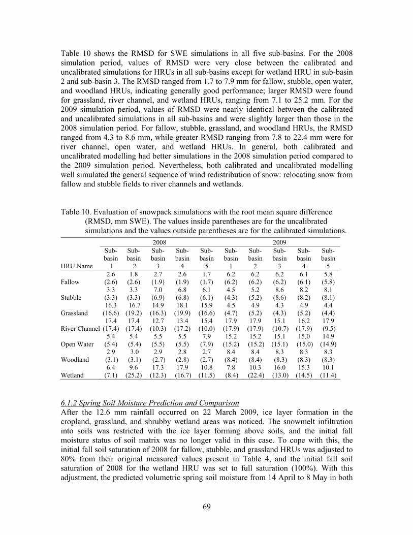
69
Table 10 shows the RMSD for SWE simulations in all five sub-basins. For the 2008 simulation period, values of RMSD were very close between the calibrated and uncalibrated simulations for HRUs in all sub-basins except for wetland HRU in sub-basin 2 and sub-basin 3. The RMSD ranged from 1.7 to 7.9 mm for fallow, stubble, open water, and woodland HRUs, indicating generally good performance; larger RMSD were found for grassland, river channel, and wetland HRUs, ranging from 7.1 to 25.2 mm. For the 2009 simulation period, values of RMSD were nearly identical between the calibrated and uncalibrated simulations in all sub-basins and were slightly larger than those in the 2008 simulation period. For fallow, stubble, grassland, and woodland HRUs, the RMSD ranged from 4.3 to 8.6 mm, while greater RMSD ranging from 7.8 to 22.4 mm were for river channel, open water, and wetland HRUs. In general, both calibrated and uncalibrated modelling had better simulations in the 2008 simulation period compared to the 2009 simulation period. Nevertheless, both calibrated and uncalibrated modelling well simulated the general sequence of wind redistribution of snow: relocating snow from fallow and stubble fields to river channels and wetlands. Table 10. Evaluation of snowpack simulations with the root mean square difference
(RMSD, mm SWE). The values inside parentheses are for the uncalibrated simulations and the values outside parentheses are for the calibrated simulations.
6.1.2 Spring Soil Moisture Prediction and Comparison After the 12.6 mm rainfall occurred on 22 March 2009, ice layer formation in the cropland, grassland, and shrubby wetland areas was noticed. The snowmelt infiltration into soils was restricted with the ice layer forming above soils, and the initial fall moisture status of soil matrix was no longer valid in this case. To cope with this, the initial fall soil saturation of 2008 for fallow, stubble, and grassland HRUs was adjusted to 80% from their original measured values present in Table 4, and the initial fall soil saturation of 2008 for the wetland HRU was set to full saturation (100%). With this adjustment, the predicted volumetric spring soil moisture from 14 April to 8 May in both
2008 2009
HRU Name
Sub-basin
1
Sub-basin
2
Sub-basin
3
Sub-basin
4
Sub-basin
5
Sub-basin
1
Sub-basin
2
Sub-basin
3
Sub-basin
4
Sub-basin
5
Fallow 2.6
(2.6) 1.8
(2.6) 2.7
(1.9) 2.6
(1.9) 1.7
(1.7) 6.2
(6.2) 6.2
(6.2) 6.2
(6.2) 6.1
(6.1) 5.8
(5.8)
Stubble 3.3
(3.3) 3.3
(3.3) 7.0
(6.9) 6.8
(6.8) 6.1
(6.1) 4.5
(4.3) 5.2
(5.2) 8.6
(8.6) 8.2
(8.2) 8.1
(8.1)
Grassland 16.3
(16.6) 16.7 (19.2)
14.9 (16.3)
18.1 (19.9)
15.9 (16.6)
4.5 (4.7)
4.9 (5.2)
4.3 (4.3)
4.9 (5.2)
4.4 (4.4)
River Channel 17.4
(17.4) 17.4
(17.4) 12.7
(10.3) 13.4
(17.2) 15.4
(10.0) 17.9
(17.9) 17.9
(17.9) 15.1
(10.7)16.2
(17.9) 17.9 (9.5)
Open Water 5.4
(5.4) 5.4
(5.4) 5.5
(5.5) 5.5
(5.5) 7.9
(7.9) 15.2
(15.2) 15.2
(15.2)15.1
(15.1) 15.0
(15.0) 14.9
(14.9)
Woodland 2.9
(3.1) 3.0
(3.1) 2.9
(2.7) 2.8
(2.8) 2.7
(2.7) 8.4
(8.4) 8.4
(8.4) 8.3
(8.3) 8.3
(8.3) 8.3
(8.3)
Wetland 6.4
(7.1) 9.6
(25.2) 17.3
(12.3) 17.9
(16.7)10.8
(11.5) 7.8
(8.4) 10.3
(22.4)16.0
(13.0)15.3
(14.5) 10.1
(11.4)

70
2008 and 2009 was tested against the observations from the main weather station (Figure 34). Earlier observations cannot be used because of partially frozen soil. Both calibrated and uncalibrated simulations had identical results; simulated values were generally higher than observed in the 2008 simulation and lower than the observed in the 2009 simulation period (Figure 34). Table 11 shows the RMSD for spring soil moisture predictions in both 2008 and 2009. The calibrated and uncalibrated had the same performance; the RMSD were 0.011 and 0.009 for 2008 and 2009, respectively, indicating on average, the difference between the observed and simulated volumetric soil moisture was 1.1% and 0.9%. This difference is within the range of variability expected from small scale variations and measurement errors.
Figure 34. Comparisons of the observed and simulated volumetric spring soil moisture
from the main weather station in the Smith Creek Research Basin. (a) 2008 simulation period and (b) 2009 simulation period.
Table 11. Evaluation of volumetric spring soil moisture predictions with the root mean
square difference (RMSD) in 2008 and 2009 simulation periods. Year Calibrated Simulation Uncalibrated Simulation 2008 0.011 0.011 2009 0.009 0.009
6.1.3 Spring Streamflow Prediction and Comparison For both calibrated and uncalibrated modelling, the simulations of spring streamflow were compared to the observations for both 2008 and 2009 simulation periods. Figure 35 shows the comparisons among the observed daily mean basin discharge and calibration and uncalibrated simulations. For the 2008 simulation period, both calibrated and uncalibrated simulations had good timing of the peak daily discharge (Figure 35(a)); the peak daily discharge was one day ahead and two days late compared to the observed one. The observed peak daily discharge was 4.65 m3 s-1, which is very comparable to the

71
calibrated (4.47 m3 s-1) and uncalibrated (4.68 m3 s-1) simulations (Table 12). On average, relatively small differences between the observed daily discharge and the simulations were found; Table 12 shows that the RMSD were 0.03 and 0.12 m3 s-1 for the calibrated and uncalibrated simulations, respectively. Both simulations predicted 27 days of spring streamflow, which is three days shorter than the observed streamflow duration. MB listed in Table 12 for the calibrated and uncalibrated simulations was -0.12 and -0.32, suggesting that the calibrated and uncalibrated simulations underestimated the cumulative basin discharge by 12% and 32%. The calibrated simulation appears to be better than the uncalibrated one, but the key parameter sdmax in the upland area was calibrated by comparing the simulated discharge to the observed one, which without doubt makes the calibrated simulation closer to the observation. On the other hand, the uncalibrated simulation used the sdmax estimated from automated processes, which are subject to cumulative errors. The underestimation of seasonal discharge and discharge at the end of the spring period suggests that additional parameterisation of drained wetlands is needed in future versions of CRHM and PHM. Table 12. Evaluation of simulating spring basin discharge with root mean square
difference (RMSD, m3 s-1), model bias (MB), peak discharge (m3 s-1), and duration of discharge (day) in 2008 and 2009 simulation periods. CS, US, and Obs are calibrated simulation, uncalibrated simulation, and observation, respectively.
RMSD (m3/s) MB
Peak Discharge (m3/s)
Duration (Day)
Year CS US CS US Obs CS US Obs CS US 2008 0.03 0.12 -0.12 -0.32 4.65 4.47 4.68 30 27 27 2009 0.27 0.33 -0.30 -0.56 6.22 6.85 6.29 40 20 20
Figure 35. Comparisons of the observed and simulated spring daily mean discharge in the
Smith Creek Research Basin. (a) 2008 simulation period and (b) 2009 simulation period.

72
For the 2009 simulation period, as explained in previous section, the starting date for major snowmelt was delayed for all HRUs and fall soil moisture status for cropland, grassland, and wetland HRUs was adjusted to high or full saturation due to the rainfall event on 22 March 2009. The calibrated simulation predicted the peak daily discharge two days earlier than the observed one, while the uncalibrated had the same timing for peak daily discharge as did the observation (Figure 35(b)). The calibrated and uncalibrated simulations of peak discharge were 6.85 and 6.29 m3 s-1, respectively, which were quite similar to the observed (i.e. 6.22 m3 s-1; Table 12). RMSD were 0.27 and 0.33 m3 s-1 for the calibrated and uncalibrated simulations, respectively, indicating that on average, the difference between the observation and calibrated simulation was slightly smaller. The simulated duration of spring streamflow was 20 days shorter than the observed one. For the cumulative basin spring discharge, the simulated magnitude was lower by 30% and 56% for the calibrated and uncalibrated simulations, respectively. The relatively large difference in the timing and the magnitude of the basin discharge between simulations and observation is attributed to the nature of representation of wetlands in the model. That is, only single type of wetland HRU was set up for the entire basin. This might be oversimplified as there are other types of wetland (e.g. drained wetland vs. intact wetland). This issue will be discussed more in the following recommendation section of this report. An additional model test was conducted using the meteorological data from Yorkton Airport, Saskatchewan with the same modelling parameters and structure. The meteorological data include hourly air temperature, relative humidity, vapour pressure, wind speed, daily precipitation, and estimated hourly incoming shortwave radiation using a simple method presented by Annandale et al. (2002). The purpose is to assess the importance and usefulness of a weather station in the basin. Figure 36 illustrates the comparisons among the calibrated and uncalibrated simulations and observations of spring daily basin discharge in 2008 and 2009 simulation periods. For the 2008 simulation period, the calibrated and uncalibrated simulated peak daily discharge was 5.73 and 5.17 m3 s-1, respectively, which was still comparable to the observed (4.65 m3 s-1; Table 13). Both simulations predicted the timing of peak daily discharge by about seven days late compared to the observation. RMSD were 0.19 and 0.13 m3 s-1 for the calibrated and uncalibrated simulations, respectively; MB present in Table 13 for the calibrated and uncalibrated simulations was 0.36 and -0.10, showing the simulations still had relatively good performance. However, for the 2009 simulation period, much higher peak daily discharge was predicted in calibrated (53.20 m3 s-1) and uncalibrated (53.20 m3 s-1) simulations shown in Figure 36(b). The timing for the peak discharge was simulated as14 days late compared to the observed. Table 13 shows large values of RMSD for the calibrated (2.45 m3 s-1) and uncalibrated (2.15 m3 s-1) simulations, and the calibrated and uncalibrated simulations overestimated the cumulative basin discharge by 438% and 375% as indicated by the values of MB. Overall, the model performance using the meteorological data from Yorkton is not acceptable even though all the model structure and parameters

73
were kept unchanged. Thus, it is important and imperative to have a station collecting weather information within the basin. Table 13. Evaluation of simulating spring basin discharge using meteorological data from
Yorkton, with root mean square difference (RMSD, m3 s-1), model bias (MB), peak discharge (m3 s-1), and duration of discharge (day) in 2008 and 2009 simulation periods. CS, US, and Obs are calibrated simulation, uncalibrated simulation, and observation, respectively.
RMSD (m3/s) MB
Peak Discharge (m3/s)
Year CS US CS US Obs CS US 2008 0.19 0.13 0.36 -0.10 4.65 5.73 5.172009 2.45 2.15 4.38 3.75 6.22 53.20 48.36
Figure 36. Comparisons of the observed and simulated spring daily mean discharge in the
Smith Creek Research Basin using meteorological data from Yorkton. (a) 2008 simulation period and (b) 2009 simulation period.
6.2 Comparison of Wetland Storage Estimation using the LiDAR V-A-h and V-A Methods 6.2.1 Assessing Volume Error for the Study Wetlands Volumes estimated by the LiDAR V-A-h method for the 11 study wetlands at SDNWA were compared to the actual volumes. The topography of each wetland varied, with relatively high topographic slope at SDNWA, so there were many area measurements extracted for each wetland. Depending on how many area measurements were obtained from the DEM, there were either one or multiple s coefficients calculated for each wetland. When using the automated method, the Visual Basic script was able to generate every possible s coefficient near-instantaneously. For each wetland, there was an s coefficient that was most accurate and produced the lowest root-mean-squared (RMS) volume error (Verr) (Figure 37(a)). However, when the actual wetland volumes are not

74
known, it is not possible to identify the most accurate s coefficient. Therefore, every possible combination of A1 and A2 were analyzed and the average s coefficient was used to estimate volume. The average volume error was 15%, ranging from 2% to 44% (Figure 37(b)).
Figure 37. LiDAR V-A-h method error assessment. (a) Minimum root-mean-squared
(RMS) volume error produced by the LiDAR V-A-h method and (b) RMS volume error produced by using an average s coefficient in the LiDAR V-A-h method.
6.2.2 Comparison between the LiDAR V-A-h to V-A Methods The maximum volume estimated by the LiDAR V-A-h method was compared to maximum volume estimated by the two V-A equations. Maximum volume estimated by the LiDAR V-A-h method was, on average, more accurate than that estimated through the Wiens (2001) and Gleason et al. (2007) V-A equations (Figure 38). When comparing the estimated volume to the actual, the Wiens equation consistently underestimated Vmax. This was most evident for wetlands at SDNWA, especially the large wetlands (Figure 38(b)). Since the equation was developed for the Upper Assiniboine River Basin, it seems

75
that the regression equation did not suite the rolling moraine topography of SDNWA. The appropriate V-A equation for SDNWA was the Prairie Coteau physiographic equation (Equation [46]). While this equation adequately estimated the volumes of large wetlands (i.e. ~4,500 m3) (Figure 38(b)), it consistently underestimated the volume of small wetlands (Figure 38(a)).
Figure 38. Volume estimated through the LiDAR V-A-h method, Wiens method and
Gleason method for (a) small and (b) large wetlands at SDNWA.

76
7. Sensitivity Analysis of Smith Creek Scenario Simulations 7.1 Scenario Description Two types of scenarios: a land use scenario and a drainage scenario were created. In the land use scenario, scenarios range from ‘complete forest cover’ to ‘primarily agricultural land use’; while ‘high natural wetland extent/poorly drained’ and ‘minimal wetland extent/well drained’ are the spectrums of the drainage scenario. The ‘complete forest cover’ scenario involves conversion of fallow and stubble fields to tree woodland; whereas grassland and tree woodland are converted to fallow and stubble in the ‘primarily agricultural land use’. The ‘high natural wetland extent/poorly drained’ scenario converts fallow and stubble to wetland and open water at the 1958 extent, and correspondingly reduces the river channel to the 1958 network. The ‘minimal wetland extent/well drained’ scenario focuses on losing wetland and open water to increase fallow and stubble fields. In both drainage scenarios, there is an alteration of channel drainage condition. 7.1.1 2007-2008 Scenario Simulations The 2007-2008 scenarios simulations were conducted in CRHM using the LiDAR-DEM derived parameters (basin area, sub-basin area, HRU area, sdmax) without any calibration. The CRHM simulation during 31 October 2007 to 8 May 2008 was used as baseline. In each scenario, four levels of change: 25%, 50%, 75%, and “extreme” full change (~100%) were generated. In addition, two stages: initial stage and mature stage were differentiated for each level of change. At the initial stage, the new target HRU inherits the original converting HRU’s surface and soil properties. For instance, when converting fallow and stubble HRUs to woodland HRU at the initial stage, the new woodland HRU would inherit properties from fallow and stubble HRUs, such as fall soil saturation (θ) and maximum surface depression storage (sdmax). Values of these parameters are based on area-weighted estimation shown in Equations [61] and [62].
_ _
_
_
( )( ) ( ) ( )
( )( ) ( ) ( )
( )( ) (
Woodland new Woodland old
Fallow old
Stubble old
Area WoodlandArea Woodland Area Fallow Area Stubble
Area FallowArea Woodland Area Fallow Area Stubble
Area StubbleArea Woodland Area
θ θ
θ
θ
=+ Δ + ΔΔ
++ Δ + ΔΔ
++ Δ ) ( )Fallow Area Stubble+ Δ
[61]
_ _
_
_
( )_ max _ max( ) ( ) ( )
( )_ max( ) ( ) ( )
( )_ max
Woodland new Woodland old
Fallow old
Stubble old
Area Woodlandsd sdArea Woodland Area Fallow Area Stubble
Area FallowsdArea Woodland Area Fallow Area Stubble
Area StubblesdA
=+ Δ + ΔΔ
++ Δ + ΔΔ
+( ) ( ) ( )rea Woodland Area Fallow Area Stubble+ Δ + Δ
[62]

77
Compared to the initial stage, the new target HRU evolves to its own properties and does not inherit the original converting HRU’s properties at the mature stage. For example, when converting fallow and stubble HRUs to woodland HRU at the mature stage, θWoodland_new = θWoodland_old and sd_maxWoodland_new = sd_maxWoodland_old. In total, 32 2007-2008 scenario simulations were created and are described in Figure 39. HRU area, fall soil saturation, and sdmax were changed and are presented in Table 14 to 17 for the initial stage scenarios of ‘complete forest cover’, ‘primarily agricultural land use’, ‘high natural wetland extent/poorly drained’, and ‘minimal wetland extent/well drained’. Table 18 to 21 show the HRU area, fall soil saturation, and sdmax for these four scenarios at the mature stage. In addition, for both drainage scenarios, channel drainage condition was altered by changing the routing distribution parameter that is discussed in the Section 5.1.5. Table 22 to 23 list the values for the routing distribution parameter between HRUs within each sub-basin. Higher values indicate more runoff is routed from other HRUs. In the scenario of ‘high natural wetland extent/poorly drained’, the routing distribution parameter for river channel HRUs ranges from 0.28 (fallow, stubble, and grassland HRUs) and 0.45 (woodland HRU) in the ‘normal case’ to 0.07 (fallow, stubble, and grassland HRUs) and 0.10 (woodland HRU) in the extreme full change level (1958 channel drainage condition). In the scenario of ‘minimal wetland extent/well drained’, the routing distribution parameter for river channel HRUs ranges from 0.28 (fallow, stubble, and grassland HRUs) and 0.45 (woodland HRU) in the ‘normal case’ to 0.40 (fallow, stubble, and grassland HRUs) and 0.86 (woodland HRU) in the complete conversion case. 7.1.2 Historical Scenarios Simulations The historical scenarios simulations were carried out in CRHM based on the LiDAR-DEM derived parameters (basin area, sub-basin area, sdmax). The current supervised land use classification was used as the basis for HRU area alteration. Meteorology during 1965-82 and 1993-2005 periods was input for the simulations; initial fall soil moisture status was estimated from the average measured data in the nearby area (i.e. Yorkton, Russell, Langenburg, and Runnymede) during these periods. Initial fall surface depression storage (sdint) during these two historical periods was approximated by using the total rainfall in September and October as an index. The purpose of the historical scenarios simulations is not to reproduce the spring basin hydrograph, but to examine the sensitivity of the spring basin discharge to the changes in land use and drainage. The flowchart of historical scenarios is shown in Figure 40. Four scenarios: ‘forest conversion’, ‘agricultural conversion’, ‘wetland restoration’, and ‘wetland drainage’ were created, and 116 scenario simulations were generated for 29-year period (i.e. 1965-82 and 1993-2005). Table 24 to 25 show the changes in HRU area and routing distribution parameter corresponding to these four scenarios.

78
Land UseSmith Creek 2007-2008 Scenarios
Drainage
Complete forest coverconverting fallow andstubble fields to treewoodland
Primarily agriculturalland useconverting grasslandand tree woodland tofallow and stubble
High natural wetlandextent/poorly drainedconverting fallow andstubble fields towetland and openwater to 1958 leveland reducing riverchannel to 1958 level
Minimal wetland extent/well drainedconverting wetland andopen water to fallowand stubble fields
25% conversion
50% conversion
75% conversion
complete (~100%) conversion
Two stages:Initial stageMature Stage
Four levels:
25% conversion
50% conversion
75% conversion
complete (~100%) conversion
Two stages:Initial stageMature Stage
Four levels:
25% conversion
50% conversion
75% conversion
complete (~100%) conversion
Two stages:Initial stageMature Stage
Four levels: 25% conversion
50% conversion
75% conversion
complete (~100%) conversion
Two stages:Initial stageMature Stage
Four levels:
Figure 39. Development of Smith Creek 2007-2008 scenarios.

79
Table 14. Changes of HRU area, fall soil saturation, and sdmax for the scenarios of ‘complete forest cover’ at the initial stage. Note that bold italic values are area-weighted estimation.
HRU Area (km2) Fall Soil Saturation (%) sdmax (mm)
Sub-basin 1 2 3 4 5 Sub-basin 1 2 3 4 5 Sub-basin 1 2 3 4 5
2007-08 Normal Case 2007-08 Normal Case 2007-08 Normal Case
fallow 6.30 1.70 2.10 3.10 0.30 fallow 46.00 46.00 46.00 46.00 46.00 fallow 61.00 67.00 69.00 67.00 69.00
stubble 121.90 31.00 34.50 21.80 6.30 stubble 50.00 50.00 50.00 50.00 50.00 stubble 61.00 67.00 69.00 67.00 69.00
woodland 49.00 12.40 12.70 9.20 3.00 woodland 53.00 53.00 53.00 53.00 53.00 woodland 78.00 86.00 90.00 88.00 87.00
25% Conversion 25% Conversion 25% Conversion
fallow 4.75 1.30 1.60 2.35 0.25 fallow 46.00 46.00 46.00 46.00 46.00 fallow 61.00 67.00 69.00 67.00 69.00
stubble 91.45 23.28 25.90 16.38 4.75 stubble 50.00 50.00 50.00 50.00 50.00 stubble 61.00 67.00 69.00 67.00 69.00
woodland 81.00 20.53 21.80 15.38 4.60 woodland 51.74 51.73 51.66 51.60 51.91 woodland 71.28 78.48 81.23 79.57 80.74
50% Conversion 50% Conversion 50% Conversion
fallow 3.20 0.90 1.10 1.60 0.20 fallow 46.00 46.00 46.00 46.00 46.00 fallow 61.00 67.00 69.00 67.00 69.00
stubble 61.00 15.55 17.30 10.95 3.20 stubble 50.00 50.00 50.00 50.00 50.00 stubble 61.00 67.00 69.00 67.00 69.00
woodland 113.00 28.65 30.90 21.55 6.20 woodland 51.19 51.19 51.10 51.00 51.39 woodland 68.37 75.22 77.63 75.97 77.71
75% Conversion 75% Conversion 75% Conversion
fallow 1.65 0.50 0.60 0.85 0.15 fallow 46.00 46.00 46.00 46.00 46.00 fallow 61.00 67.00 69.00 67.00 69.00
stubble 30.55 7.83 8.70 5.53 1.65 stubble 50.00 50.00 50.00 50.00 50.00 stubble 61.00 67.00 69.00 67.00 69.00
woodland 145.00 36.78 40.00 27.73 7.80 woodland 50.89 50.88 50.80 50.67 51.08 woodland 66.74 73.41 75.67 73.97 75.92
Complete (~100%) Conversion Complete (~100%) Conversion Complete (~100%) Conversion
fallow 0.10 0.10 0.10 0.10 0.10 fallow 46.00 46.00 46.00 46.00 46.00 fallow 61.00 67.00 69.00 67.00 69.00
stubble 0.10 0.10 0.10 0.10 0.10 stubble 50.00 50.00 50.00 50.00 50.00 stubble 61.00 67.00 69.00 67.00 69.00
woodland 177.00 44.90 49.10 33.90 9.40 woodland 50.69 50.69 50.61 50.46 50.87 woodland 65.71 72.25 74.43 72.70 74.74

80
Table 15. Changes of HRU area, fall soil saturation, and sdmax for the scenarios of ‘primarily agricultural land use’ at the initial stage. Note that bold italic values are area-weighted estimation.
HRU Area (km2) Fall Soil Saturation (%) sdmax (mm)
Sub-basin 1 2 3 4 5 Sub-basin 1 2 3 4 5 Sub-basin 1 2 3 4 5
2007-08 Normal Case 2007-08 Normal Case 2007-08 Normal Case
fallow 6.30 1.70 2.10 3.10 0.30 fallow 46.00 46.00 46.00 46.00 46.00 fallow 61.00 67.00 69.00 67.00 69.00
stubble 121.90 31.00 34.50 21.80 6.30 stubble 50.00 50.00 50.00 50.00 50.00 stubble 61.00 67.00 69.00 67.00 69.00
grassland 22.60 2.80 5.50 1.40 0.70 grassland 54.00 54.00 54.00 54.00 54.00 grassland 86.00 100.00 95.00 104.00 102.00
woodland 49.00 12.40 12.70 9.20 3.00 woodland 53.00 53.00 53.00 53.00 53.00 woodland 78.00 86.00 90.00 88.00 87.00
25% Conversion 25% Conversion 25% Conversion
fallow 7.41 1.93 2.38 3.26 0.35 fallow 47.09 46.86 46.86 46.35 47.10 fallow 63.92 69.59 71.64 68.14 72.15
stubble 138.64 34.52 38.72 24.24 7.12 stubble 50.40 50.32 50.36 50.31 50.37 stubble 63.36 69.19 71.45 69.31 71.37
grassland 16.98 2.13 4.15 1.08 0.55 grassland 54.00 54.00 54.00 54.00 54.00 grassland 86.00 100.00 95.00 104.00 102.00
woodland 36.78 9.33 9.55 6.93 2.28 woodland 53.00 53.00 53.00 53.00 53.00 woodland 78.00 86.00 90.00 88.00 87.00
50% Conversion 50% Conversion 50% Conversion
fallow 8.51 2.17 2.66 3.42 0.41 fallow 47.90 47.54 47.53 46.67 47.91 fallow 66.08 71.62 73.72 69.17 74.46
stubble 155.39 38.03 42.94 26.68 7.94 stubble 50.71 50.59 50.65 50.57 50.66 stubble 65.21 70.98 73.42 71.21 73.25
grassland 11.35 1.45 2.80 0.75 0.40 grassland 54.00 54.00 54.00 54.00 54.00 grassland 86.00 100.00 95.00 104.00 102.00
woodland 24.55 6.25 6.40 4.65 1.55 woodland 53.00 53.00 53.00 53.00 53.00 woodland 78.00 86.00 90.00 88.00 87.00
75% Conversion 75% Conversion 75% Conversion
fallow 9.62 2.40 2.94 3.58 0.46 fallow 48.53 48.09 48.08 46.96 48.52 fallow 67.74 73.26 75.41 70.10 76.24
stubble 172.13 41.55 47.16 29.12 8.76 stubble 50.97 50.81 50.89 50.79 50.89 stubble 66.70 72.47 75.04 72.78 74.78
grassland 5.73 0.78 1.45 0.43 0.25 grassland 54.00 54.00 54.00 54.00 54.00 grassland 86.00 100.00 95.00 104.00 102.00
woodland 12.33 3.18 3.25 2.38 0.83 woodland 53.00 53.00 53.00 53.00 53.00 woodland 78.00 86.00 90.00 88.00 87.00
Complete (~100%) Conversion Complete (~100%) Conversion Complete (~100%) Conversion
fallow 10.73 2.63 3.22 3.74 0.52 fallow 49.02 48.54 48.53 47.23 49.01 fallow 69.06 74.61 76.81 70.96 77.64
stubble 188.87 45.07 51.38 31.56 9.58 stubble 51.18 50.99 51.08 50.97 51.09 stubble 67.92 73.72 76.39 74.11 76.05
grassland 0.10 0.10 0.10 0.10 0.10 grassland 54.00 54.00 54.00 54.00 54.00 grassland 86.00 100.00 95.00 104.00 102.00
woodland 0.10 0.10 0.10 0.10 0.10 woodland 53.00 53.00 53.00 53.00 53.00 woodland 78.00 86.00 90.00 88.00 87.00

81
Table 16. Changes of HRU area, fall soil saturation, and sdmax for the scenarios of ‘high natural wetland extent/poorly drained’ at the initial stage. Note that bold italic values are area-weighted estimation.
HRU Area (km2) Fall Soil Saturation (%) sdmax (mm)
Sub-basin 1 2 3 4 5 Sub-basin 1 2 3 4 5 Sub-basin 1 2 3 4 5
2007-08 Normal Case 2007-08 Normal Case 2007-08 Normal Case
fallow 6.30 1.70 2.10 3.10 0.30 fallow 46.00 46.00 46.00 46.00 46.00 fallow 61.00 67.00 69.00 67.00 69.00
stubble 121.90 31.00 34.50 21.80 6.30 stubble 50.00 50.00 50.00 50.00 50.00 stubble 61.00 67.00 69.00 67.00 69.00
wetland 23.20 2.60 2.70 1.80 0.50 wetland 87.00 87.00 87.00 87.00 87.00 wetland 317.00 374.00 395.00 386.00 366.00
open water 10.50 1.00 0.50 0.40 0.10 open water 100.00 100.00 100.00 100.00 100.00 open water 317.00 374.00 395.00 386.00 366.00
river channel 0.80 0.20 0.50 0.20 0.10 river channel 100.00 100.00 100.00 100.00 100.00 river channel 200.00 200.00 200.00 200.00 200.00
25% Conversion 25% Conversion 25% Conversion
fallow 5.90 1.61 1.90 3.02 0.28 fallow 46.00 46.00 46.00 46.00 46.00 fallow 61.00 67.00 69.00 67.00 69.00
stubble 115.92 29.60 31.47 20.56 5.94 stubble 50.00 50.00 50.00 50.00 50.00 stubble 61.00 67.00 69.00 67.00 69.00
wetland 27.79 3.67 5.03 2.75 0.78 wetland 80.64 75.85 69.10 73.76 72.96 wetland 274.49 284.23 243.16 275.63 258.46
open water 12.47 1.46 1.50 0.81 0.22 open water 100.00 100.00 100.00 100.00 100.00 open water 276.39 277.19 176.53 224.70 202.59
river channel 0.63 0.17 0.41 0.17 0.09 river channel 100.00 100.00 100.00 100.00 100.00 river channel 200.00 200.00 200.00 200.00 200.00
50% Conversion 50% Conversion 50% Conversion
fallow 5.51 1.51 1.70 2.94 0.25 fallow 46.00 46.00 46.00 46.00 46.00 fallow 61.00 67.00 69.00 67.00 69.00
stubble 109.93 28.20 28.44 19.33 5.58 stubble 50.00 50.00 50.00 50.00 50.00 stubble 61.00 67.00 69.00 67.00 69.00
wetland 32.37 4.74 7.36 3.69 1.06 wetland 76.08 69.73 62.53 67.31 66.34 wetland 244.03 234.93 187.43 221.78 207.73
open water 14.43 1.92 2.50 1.21 0.34 open water 100.00 100.00 100.00 100.00 100.00 open water 246.85 226.63 132.75 171.37 154.53
river channel 0.46 0.14 0.31 0.14 0.07 river channel 100.00 100.00 100.00 100.00 100.00 river channel 200.00 200.00 200.00 200.00 200.00
75% Conversion 75% Conversion 75% Conversion
fallow 5.11 1.42 1.50 2.85 0.23 fallow 46.00 46.00 46.00 46.00 46.00 fallow 61.00 67.00 69.00 67.00 69.00
stubble 103.95 26.80 25.41 18.09 5.22 stubble 50.00 50.00 50.00 50.00 50.00 stubble 61.00 67.00 69.00 67.00 69.00
wetland 36.96 5.80 9.68 4.64 1.34 wetland 72.66 65.86 59.11 63.48 62.48 wetland 221.13 203.77 158.48 189.90 178.20
open water 16.40 2.37 3.49 1.62 0.46 open water 100.00 100.00 100.00 100.00 100.00 open water 224.38 195.57 113.98 144.80 131.54
river channel 0.29 0.10 0.22 0.10 0.06 river channel 100.00 100.00 100.00 100.00 100.00 river channel 200.00 200.00 200.00 200.00 200.00
Complete (~100%) Conversion Complete (~100%) Conversion Complete (~100%) Conversion
fallow 4.72 1.33 1.30 2.77 0.20 fallow 46.00 46.00 46.00 46.00 46.00 fallow 61.00 67.00 69.00 67.00 69.00
stubble 97.96 25.40 22.38 16.86 4.86 stubble 50.00 50.00 50.00 50.00 50.00 stubble 61.00 67.00 69.00 67.00 69.00
wetland 41.00 6.60 12.00 5.30 1.80 wetland 70.91 65.77 57.07 64.18 53.96 wetland 205.95 189.76 140.88 177.73 142.99
open water 18.90 3.10 4.50 2.30 0.40 open water 100.00 100.00 100.00 100.00 100.00 open water 200.82 159.35 103.32 113.19 171.20
river channel 0.12 0.07 0.12 0.07 0.04 river channel 100.00 100.00 100.00 100.00 100.00 river channel 200.00 200.00 200.00 200.00 200.00

82
Table 17. Changes of HRU area, fall soil saturation, and sdmax for the scenarios of ‘minimal wetland extent/well drained’ at the initial stage. Note that bold italic values are area-weighted estimation.
HRU Area (km2) Fall Soil Saturation (%) sdmax (mm)
Sub-basin 1 2 3 4 5 Sub-basin 1 2 3 4 5 Sub-basin 1 2 3 4 5
2007-08 Normal Case 2007-08 Normal Case 2007-08 Normal Case
fallow 6.30 1.70 2.10 3.10 0.30 fallow 46.00 46.00 46.00 46.00 46.00 fallow 61.00 67.00 69.00 67.00 69.00
stubble 121.90 31.00 34.50 21.80 6.30 stubble 50.00 50.00 50.00 50.00 50.00 stubble 61.00 67.00 69.00 67.00 69.00
wetland 23.20 2.60 2.70 1.80 0.50 wetland 87.00 87.00 87.00 87.00 87.00 wetland 317.00 374.00 395.00 386.00 366.00
open water 10.50 1.00 0.50 0.40 0.10 open water 100.00 100.00 100.00 100.00 100.00 open water 317.00 374.00 395.00 386.00 366.00
25% Conversion 25% Conversion 25% Conversion
fallow 6.82 1.75 2.15 3.13 0.31 fallow 49.43 47.34 46.93 46.43 46.83 fallow 80.50 76.23 76.06 70.16 75.02
stubble 129.76 31.80 35.20 22.27 6.39 stubble 52.48 51.01 50.77 50.82 50.54 stubble 76.50 74.70 75.51 73.72 73.36
wetland 17.43 1.98 2.05 1.38 0.40 wetland 87.00 87.00 87.00 87.00 87.00 wetland 317.00 374.00 395.00 386.00 366.00
open water 7.90 0.78 0.40 0.33 0.10 open water 100.00 100.00 100.00 100.00 100.00 open water 317.00 374.00 395.00 386.00 366.00
50% Conversion 50% Conversion 50% Conversion
fallow 7.34 1.81 2.19 3.16 0.31 fallow 52.37 48.60 47.81 46.84 47.63 fallow 97.24 84.93 82.83 73.26 80.79
stubble 137.61 32.59 35.91 22.74 6.49 stubble 54.69 51.98 51.52 51.61 51.07 stubble 90.23 82.02 81.77 80.16 77.59
wetland 11.65 1.35 1.40 0.95 0.30 wetland 87.00 87.00 87.00 87.00 87.00 wetland 317.00 374.00 395.00 386.00 366.00
open water 5.30 0.55 0.30 0.25 0.10 open water 100.00 100.00 100.00 100.00 100.00 open water 317.00 374.00 395.00 386.00 366.00
75% Conversion 75% Conversion 75% Conversion
fallow 7.86 1.86 2.24 3.19 0.32 fallow 54.93 49.78 48.66 47.25 48.39 fallow 111.76 93.13 89.31 76.29 86.34
stubble 145.47 33.39 36.61 23.21 6.58 stubble 56.65 52.90 52.23 52.36 51.58 stubble 102.47 88.99 87.79 86.34 81.70
wetland 5.88 0.73 0.75 0.53 0.20 wetland 87.00 87.00 87.00 87.00 87.00 wetland 317.00 374.00 395.00 386.00 366.00
open water 2.70 0.33 0.20 0.18 0.10 open water 100.00 100.00 100.00 100.00 100.00 open water 317.00 374.00 395.00 386.00 366.00
Complete (~100%) Conversion Complete (~100%) Conversion Complete (~100%) Conversion
fallow 8.38 1.91 2.29 3.22 0.32 fallow 57.17 50.90 49.48 47.65 49.13 fallow 124.48 100.88 95.53 79.27 91.68
stubble 153.32 34.19 37.31 23.68 6.68 stubble 58.41 53.77 52.92 53.09 52.08 stubble 113.47 95.64 93.58 92.28 85.69
wetland 0.10 0.10 0.10 0.10 0.10 wetland 87.00 87.00 87.00 87.00 87.00 wetland 317.00 374.00 395.00 386.00 366.00
open water 0.10 0.10 0.10 0.10 0.10 open water 100.00 100.00 100.00 100.00 100.00 open water 317.00 374.00 395.00 386.00 366.00

83
Table 18. Changes of HRU area, fall soil saturation, and sdmax for the scenarios of ‘complete forest cover’ at the mature stage. HRU Area (km2) Fall Soil Saturation (%) sdmax (mm)
Sub-basin 1 2 3 4 5 Sub-basin 1 2 3 4 5 Sub-basin 1 2 3 4 5
2007-08 Normal Case 2007-08 Normal Case 2007-08 Normal Case
fallow 6.30 1.70 2.10 3.10 0.30 fallow 46.00 46.00 46.00 46.00 46.00 fallow 61.00 67.00 69.00 67.00 69.00
stubble 121.90 31.00 34.50 21.80 6.30 stubble 50.00 50.00 50.00 50.00 50.00 stubble 61.00 67.00 69.00 67.00 69.00
woodland 49.00 12.40 12.70 9.20 3.00 woodland 53.00 53.00 53.00 53.00 53.00 woodland 78.00 86.00 90.00 88.00 87.00
25% Conversion 25% Conversion 25% Conversion
fallow 4.75 1.30 1.60 2.35 0.25 fallow 46.00 46.00 46.00 46.00 46.00 fallow 61.00 67.00 69.00 67.00 69.00
stubble 91.45 23.28 25.90 16.38 4.75 stubble 50.00 50.00 50.00 50.00 50.00 stubble 61.00 67.00 69.00 67.00 69.00
woodland 81.00 20.53 21.80 15.38 4.60 woodland 53.00 53.00 53.00 53.00 53.00 woodland 78.00 86.00 90.00 88.00 87.00
50% Conversion 50% Conversion 50% Conversion
fallow 3.20 0.90 1.10 1.60 0.20 fallow 46.00 46.00 46.00 46.00 46.00 fallow 61.00 67.00 69.00 67.00 69.00
stubble 61.00 15.55 17.30 10.95 3.20 stubble 50.00 50.00 50.00 50.00 50.00 stubble 61.00 67.00 69.00 67.00 69.00
woodland 113.00 28.65 30.90 21.55 6.20 woodland 53.00 53.00 53.00 53.00 53.00 woodland 78.00 86.00 90.00 88.00 87.00
75% Conversion 75% Conversion 75% Conversion
fallow 1.65 0.50 0.60 0.85 0.15 fallow 46.00 46.00 46.00 46.00 46.00 fallow 61.00 67.00 69.00 67.00 69.00
stubble 30.55 7.83 8.70 5.53 1.65 stubble 50.00 50.00 50.00 50.00 50.00 stubble 61.00 67.00 69.00 67.00 69.00
woodland 145.00 36.78 40.00 27.73 7.80 woodland 53.00 53.00 53.00 53.00 53.00 woodland 78.00 86.00 90.00 88.00 87.00
Complete (~100%) Conversion Complete (~100%) Conversion Complete (~100%) Conversion
fallow 0.10 0.10 0.10 0.10 0.10 fallow 46.00 46.00 46.00 46.00 46.00 fallow 61.00 67.00 69.00 67.00 69.00
stubble 0.10 0.10 0.10 0.10 0.10 stubble 50.00 50.00 50.00 50.00 50.00 stubble 61.00 67.00 69.00 67.00 69.00
woodland 177.00 44.90 49.10 33.90 9.40 woodland 53.00 53.00 53.00 53.00 53.00 woodland 78.00 86.00 90.00 88.00 87.00

84
Table 19. Changes of HRU area, fall soil saturation, and sdmax for the scenarios of ‘primarily agricultural land use’ at the mature stage. HRU Area (km2) Fall Soil Saturation (%) sdmax (mm)
Sub-basin 1 2 3 4 5 Sub-basin 1 2 3 4 5 Sub-basin 1 2 3 4 5
2007-08 Normal Case 2007-08 Normal Case 2007-08 Normal Case
fallow 6.30 1.70 2.10 3.10 0.30 fallow 46.00 46.00 46.00 46.00 46.00 fallow 61.00 67.00 69.00 67.00 69.00
stubble 121.90 31.00 34.50 21.80 6.30 stubble 50.00 50.00 50.00 50.00 50.00 stubble 61.00 67.00 69.00 67.00 69.00
grassland 22.60 2.80 5.50 1.40 0.70 grassland 54.00 54.00 54.00 54.00 54.00 grassland 86.00 100.00 95.00 104.00 102.00
woodland 49.00 12.40 12.70 9.20 3.00 woodland 53.00 53.00 53.00 53.00 53.00 woodland 78.00 86.00 90.00 88.00 87.00
25% Conversion 25% Conversion 25% Conversion
fallow 7.41 1.93 2.38 3.26 0.35 fallow 46.00 46.00 46.00 46.00 46.00 fallow 61.00 67.00 69.00 67.00 69.00
stubble 138.64 34.52 38.72 24.24 7.12 stubble 50.00 50.00 50.00 50.00 50.00 stubble 61.00 67.00 69.00 67.00 69.00
grassland 16.98 2.13 4.15 1.08 0.55 grassland 54.00 54.00 54.00 54.00 54.00 grassland 86.00 100.00 95.00 104.00 102.00
woodland 36.78 9.33 9.55 6.93 2.28 woodland 53.00 53.00 53.00 53.00 53.00 woodland 78.00 86.00 90.00 88.00 87.00
50% Conversion 50% Conversion 50% Conversion
fallow 8.51 2.17 2.66 3.42 0.41 fallow 46.00 46.00 46.00 46.00 46.00 fallow 61.00 67.00 69.00 67.00 69.00
stubble 155.39 38.03 42.94 26.68 7.94 stubble 50.00 50.00 50.00 50.00 50.00 stubble 61.00 67.00 69.00 67.00 69.00
grassland 11.35 1.45 2.80 0.75 0.40 grassland 54.00 54.00 54.00 54.00 54.00 grassland 86.00 100.00 95.00 104.00 102.00
woodland 24.55 6.25 6.40 4.65 1.55 woodland 53.00 53.00 53.00 53.00 53.00 woodland 78.00 86.00 90.00 88.00 87.00
75% Conversion 75% Conversion 75% Conversion
fallow 9.62 2.40 2.94 3.58 0.46 fallow 46.00 46.00 46.00 46.00 46.00 fallow 61.00 67.00 69.00 67.00 69.00
stubble 172.13 41.55 47.16 29.12 8.76 stubble 50.00 50.00 50.00 50.00 50.00 stubble 61.00 67.00 69.00 67.00 69.00
grassland 5.73 0.78 1.45 0.43 0.25 grassland 54.00 54.00 54.00 54.00 54.00 grassland 86.00 100.00 95.00 104.00 102.00
woodland 12.33 3.18 3.25 2.38 0.83 woodland 53.00 53.00 53.00 53.00 53.00 woodland 78.00 86.00 90.00 88.00 87.00
Complete (~100%) Conversion Complete (~100%) Conversion Complete (~100%) Conversion
fallow 10.73 2.63 3.22 3.74 0.52 fallow 46.00 46.00 46.00 46.00 46.00 fallow 61.00 67.00 69.00 67.00 69.00
stubble 188.87 45.07 51.38 31.56 9.58 stubble 50.00 50.00 50.00 50.00 50.00 stubble 61.00 67.00 69.00 67.00 69.00
grassland 0.10 0.10 0.10 0.10 0.10 grassland 54.00 54.00 54.00 54.00 54.00 grassland 86.00 100.00 95.00 104.00 102.00
woodland 0.10 0.10 0.10 0.10 0.10 woodland 53.00 53.00 53.00 53.00 53.00 woodland 78.00 86.00 90.00 88.00 87.00
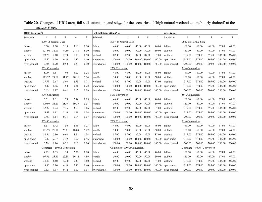
85
Table 20. Changes of HRU area, fall soil saturation, and sdmax for the scenarios of ‘high natural wetland extent/poorly drained’ at the mature stage.
HRU Area (km2) Fall Soil Saturation (%) sdmax (mm)
Sub-basin 1 2 3 4 5 Sub-basin 1 2 3 4 5 Sub-basin 1 2 3 4 5
2007-08 Normal Case 2007-08 Normal Case 2007-08 Normal Case
fallow 6.30 1.70 2.10 3.10 0.30 fallow 46.00 46.00 46.00 46.00 46.00 fallow 61.00 67.00 69.00 67.00 69.00
stubble 121.90 31.00 34.50 21.80 6.30 stubble 50.00 50.00 50.00 50.00 50.00 stubble 61.00 67.00 69.00 67.00 69.00
wetland 23.20 2.60 2.70 1.80 0.50 wetland 87.00 87.00 87.00 87.00 87.00 wetland 317.00 374.00 395.00 386.00 366.00
open water 10.50 1.00 0.50 0.40 0.10 open water 100.00 100.00 100.00 100.00 100.00 open water 317.00 374.00 395.00 386.00 366.00
river channel 0.80 0.20 0.50 0.20 0.10 river channel 100.00 100.00 100.00 100.00 100.00 river channel 200.00 200.00 200.00 200.00 200.00
25% Conversion 25% Conversion 25% Conversion
fallow 5.90 1.61 1.90 3.02 0.28 fallow 46.00 46.00 46.00 46.00 46.00 fallow 61.00 67.00 69.00 67.00 69.00
stubble 115.92 29.60 31.47 20.56 5.94 stubble 50.00 50.00 50.00 50.00 50.00 stubble 61.00 67.00 69.00 67.00 69.00
wetland 27.79 3.67 5.03 2.75 0.78 wetland 87.00 87.00 87.00 87.00 87.00 wetland 317.00 374.00 395.00 386.00 366.00
open water 12.47 1.46 1.50 0.81 0.22 open water 100.00 100.00 100.00 100.00 100.00 open water 317.00 374.00 395.00 386.00 366.00
river channel 0.63 0.17 0.41 0.17 0.09 river channel 100.00 100.00 100.00 100.00 100.00 river channel 200.00 200.00 200.00 200.00 200.00
50% Conversion 50% Conversion 50% Conversion
fallow 5.51 1.51 1.70 2.94 0.25 fallow 46.00 46.00 46.00 46.00 46.00 fallow 61.00 67.00 69.00 67.00 69.00
stubble 109.93 28.20 28.44 19.33 5.58 stubble 50.00 50.00 50.00 50.00 50.00 stubble 61.00 67.00 69.00 67.00 69.00
wetland 32.37 4.74 7.36 3.69 1.06 wetland 87.00 87.00 87.00 87.00 87.00 wetland 317.00 374.00 395.00 386.00 366.00
open water 14.43 1.92 2.50 1.21 0.34 open water 100.00 100.00 100.00 100.00 100.00 open water 317.00 374.00 395.00 386.00 366.00
river channel 0.46 0.14 0.31 0.14 0.07 river channel 100.00 100.00 100.00 100.00 100.00 river channel 200.00 200.00 200.00 200.00 200.00
75% Conversion 75% Conversion 75% Conversion
fallow 5.11 1.42 1.50 2.85 0.23 fallow 46.00 46.00 46.00 46.00 46.00 fallow 61.00 67.00 69.00 67.00 69.00
stubble 103.95 26.80 25.41 18.09 5.22 stubble 50.00 50.00 50.00 50.00 50.00 stubble 61.00 67.00 69.00 67.00 69.00
wetland 36.96 5.80 9.68 4.64 1.34 wetland 87.00 87.00 87.00 87.00 87.00 wetland 317.00 374.00 395.00 386.00 366.00
open water 16.40 2.37 3.49 1.62 0.46 open water 100.00 100.00 100.00 100.00 100.00 open water 317.00 374.00 395.00 386.00 366.00
river channel 0.29 0.10 0.22 0.10 0.06 river channel 100.00 100.00 100.00 100.00 100.00 river channel 200.00 200.00 200.00 200.00 200.00
Complete (~100%) Conversion Complete (~100%) Conversion Complete (~100%) Conversion
fallow 4.72 1.33 1.30 2.77 0.20 fallow 46.00 46.00 46.00 46.00 46.00 fallow 61.00 67.00 69.00 67.00 69.00
stubble 97.96 25.40 22.38 16.86 4.86 stubble 50.00 50.00 50.00 50.00 50.00 stubble 61.00 67.00 69.00 67.00 69.00
wetland 41.00 6.60 12.00 5.30 1.80 wetland 87.00 87.00 87.00 87.00 87.00 wetland 317.00 374.00 395.00 386.00 366.00
open water 18.90 3.10 4.50 2.30 0.40 open water 100.00 100.00 100.00 100.00 100.00 open water 317.00 374.00 395.00 386.00 366.00
river channel 0.12 0.07 0.12 0.07 0.04 river channel 100.00 100.00 100.00 100.00 100.00 river channel 200.00 200.00 200.00 200.00 200.00

86
Table 21. Changes of HRU area, fall soil saturation, and sdmax for the scenarios of ‘minimal wetland extent/well drained’ at the mature stage.
HRU Area (km2) Fall Soil Saturation (%) sdmax (mm)
Sub-basin 1 2 3 4 5 Sub-basin 1 2 3 4 5 Sub-basin 1 2 3 4 5
2007-08 Normal Case 2007-08 Normal Case 2007-08 Normal Case
fallow 6.30 1.70 2.10 3.10 0.30 fallow 46.00 46.00 46.00 46.00 46.00 fallow 61.00 67.00 69.00 67.00 69.00
stubble 121.90 31.00 34.50 21.80 6.30 stubble 50.00 50.00 50.00 50.00 50.00 stubble 61.00 67.00 69.00 67.00 69.00
wetland 23.20 2.60 2.70 1.80 0.50 wetland 87.00 87.00 87.00 87.00 87.00 wetland 317.00 374.00 395.00 386.00 366.00
open water 10.50 1.00 0.50 0.40 0.10 open water 100.00 100.00 100.00 100.00 100.00 open water 317.00 374.00 395.00 386.00 366.00
25% Conversion 25% Conversion 25% Conversion
fallow 6.82 1.75 2.15 3.13 0.31 fallow 46.00 46.00 46.00 46.00 46.00 fallow 61.00 67.00 69.00 67.00 69.00
stubble 129.76 31.80 35.20 22.27 6.39 stubble 50.00 50.00 50.00 50.00 50.00 stubble 61.00 67.00 69.00 67.00 69.00
wetland 17.43 1.98 2.05 1.38 0.40 wetland 87.00 87.00 87.00 87.00 87.00 wetland 317.00 374.00 395.00 386.00 366.00
open water 7.90 0.78 0.40 0.33 0.10 open water 100.00 100.00 100.00 100.00 100.00 open water 317.00 374.00 395.00 386.00 366.00
50% Conversion 50% Conversion 50% Conversion
fallow 7.34 1.81 2.19 3.16 0.31 fallow 46.00 46.00 46.00 46.00 46.00 fallow 61.00 67.00 69.00 67.00 69.00
stubble 137.61 32.59 35.91 22.74 6.49 stubble 50.00 50.00 50.00 50.00 50.00 stubble 61.00 67.00 69.00 67.00 69.00
wetland 11.65 1.35 1.40 0.95 0.30 wetland 87.00 87.00 87.00 87.00 87.00 wetland 317.00 374.00 395.00 386.00 366.00
open water 5.30 0.55 0.30 0.25 0.10 open water 100.00 100.00 100.00 100.00 100.00 open water 317.00 374.00 395.00 386.00 366.00
75% Conversion 75% Conversion 75% Conversion
fallow 7.86 1.86 2.24 3.19 0.32 fallow 46.00 46.00 46.00 46.00 46.00 fallow 61.00 67.00 69.00 67.00 69.00
stubble 145.47 33.39 36.61 23.21 6.58 stubble 50.00 50.00 50.00 50.00 50.00 stubble 61.00 67.00 69.00 67.00 69.00
wetland 5.88 0.73 0.75 0.53 0.20 wetland 87.00 87.00 87.00 87.00 87.00 wetland 317.00 374.00 395.00 386.00 366.00
open water 2.70 0.33 0.20 0.18 0.10 open water 100.00 100.00 100.00 100.00 100.00 open water 317.00 374.00 395.00 386.00 366.00
Complete (~100%) Conversion Complete (~100%) Conversion Complete (~100%) Conversion
fallow 8.38 1.91 2.29 3.22 0.32 fallow 46.00 46.00 46.00 46.00 46.00 fallow 61.00 67.00 69.00 67.00 69.00
stubble 153.32 34.19 37.31 23.68 6.68 stubble 50.00 50.00 50.00 50.00 50.00 stubble 61.00 67.00 69.00 67.00 69.00
wetland 0.10 0.10 0.10 0.10 0.10 wetland 87.00 87.00 87.00 87.00 87.00 wetland 317.00 374.00 395.00 386.00 366.00
open water 0.10 0.10 0.10 0.10 0.10 open water 100.00 100.00 100.00 100.00 100.00 open water 317.00 374.00 395.00 386.00 366.00

87
Table 22. Changes of routing distribution parameter between HRUs within the sub-basins for the initial and mature stage scenarios of ‘high natural wetland extent/poorly drained’.
HRU fallow stubble grassland river channel open water woodland wetland 2007-08 Normal Case fallow 0 0 0 0.28 0.13 0.38 0.21 stubble 0 0 0 0.28 0.13 0.38 0.21 grassland 0 0 0 0.28 0.13 0.38 0.21 open water 0 0 0 1 0 0 0 woodland 0 0 0 0.45 0.21 0 0.34 wetland 0 0 0 0 1 0 0 river channel 0 0 0 0 0 0 0 25% Conversion fallow 0 0 0 0.22 0.15 0.38 0.25 stubble 0 0 0 0.22 0.15 0.38 0.25 grassland 0 0 0 0.22 0.15 0.38 0.25 open water 0 0 0 1 0 0 0 woodland 0 0 0 0.36 0.24 0 0.39 wetland 0 0 0 0 1 0 0 river channel 0 0 0 0 0 0 0 50% Conversion fallow 0 0 0 0.16 0.18 0.37 0.29 stubble 0 0 0 0.16 0.18 0.37 0.29 grassland 0 0 0 0.16 0.18 0.37 0.29 open water 0 0 0 1 0 0 0 woodland 0 0 0 0.26 0.28 0 0.46 wetland 0 0 0 0 1 0 0 river channel 0 0 0 0 0 0 0 75% Conversion fallow 0 0 0 0.14 0.16 0.45 0.25 stubble 0 0 0 0.14 0.16 0.45 0.25 grassland 0 0 0 0.14 0.16 0.45 0.25 open water 0 0 0 1 0 0 0 woodland 0 0 0 0.25 0.28 0 0.46 wetland 0 0 0 0 1 0 0 river channel 0 0 0 0 0 0 0 Complete (~100%) Conversion fallow 0 0 0 0.07 0.24 0.31 0.38 stubble 0 0 0 0.07 0.24 0.31 0.38 grassland 0 0 0 0.07 0.24 0.31 0.38 open water 0 0 0 1 0 0 0 woodland 0 0 0 0.10 0.35 0 0.55 wetland 0 0 0 0 1 0 0 river channel 0 0 0 0 0 0 0

88
Table 23. Changes of routing distribution parameter between HRUs within the sub-basins for the initial and mature stage scenarios of ‘minimal wetland extent/well drained’.
HRU fallow stubble grassland river channel open water woodland wetland 2007-08 Normal Case fallow 0 0 0 0.28 0.13 0.38 0.21 stubble 0 0 0 0.28 0.13 0.38 0.21 grassland 0 0 0 0.28 0.13 0.38 0.21 open water 0 0 0 1 0 0 0 woodland 0 0 0 0.45 0.21 0 0.34 wetland 0 0 0 0 1 0 0 river channel 0 0 0 0 0 0 0 25% Conversion fallow 0 0 0 0.30 0.12 0.39 0.19 stubble 0 0 0 0.30 0.12 0.39 0.19 grassland 0 0 0 0.30 0.12 0.39 0.19 open water 0 0 0 1 0 0 0 woodland 0 0 0 0.49 0.20 0 0.32 wetland 0 0 0 0 1 0 0 river channel 0 0 0 0 0 0 0 50% Conversion fallow 0 0 0 0.32 0.10 0.41 0.17 stubble 0 0 0 0.32 0.10 0.41 0.17 grassland 0 0 0 0.32 0.10 0.41 0.17 open water 0 0 0 1 0 0 0 woodland 0 0 0 0.54 0.18 0 0.28 wetland 0 0 0 0 1 0 0 river channel 0 0 0 0 0 0 0 75% Conversion fallow 0 0 0 0.34 0.08 0.45 0.13 stubble 0 0 0 0.34 0.08 0.45 0.13 grassland 0 0 0 0.34 0.08 0.45 0.13 open water 0 0 0 1 0 0 0 woodland 0 0 0 0.62 0.15 0 0.23 wetland 0 0 0 0 1 0 0 river channel 0 0 0 0 0 0 0 Complete (~100%) Conversion fallow 0 0 0 0.40 0.03 0.53 0.03 stubble 0 0 0 0.40 0.03 0.53 0.03 grassland 0 0 0 0.40 0.03 0.53 0.03 open water 0 0 0 1 0 0 0 woodland 0 0 0 0.86 0.07 0 0.07 wetland 0 0 0 0 1 0 0 river channel 0 0 0 0 0 0 0
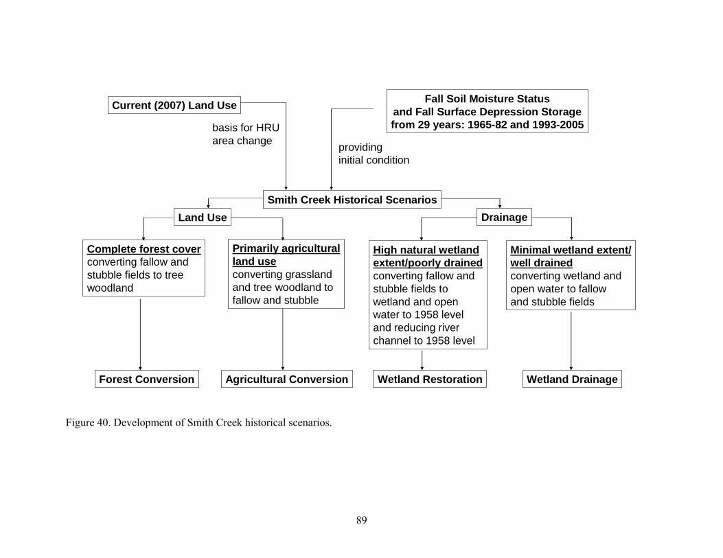
89
Land UseSmith Creek Historical Scenarios
Drainage
Complete forest coverconverting fallow andstubble fields to treewoodland
Primarily agriculturalland useconverting grasslandand tree woodland tofallow and stubble
High natural wetlandextent/poorly drainedconverting fallow andstubble fields towetland and openwater to 1958 leveland reducing riverchannel to 1958 level
Minimal wetland extent/well drainedconverting wetland andopen water to fallowand stubble fields
Forest Conversion Agricultural Conversion Wetland Restoration Wetland Drainage
Current (2007) Land Use Fall Soil Moisture Statusand Fall Surface Depression Storagefrom 29 years: 1965-82 and 1993-2005basis for HRU
area change providinginitial condition
Figure 40. Development of Smith Creek historical scenarios.
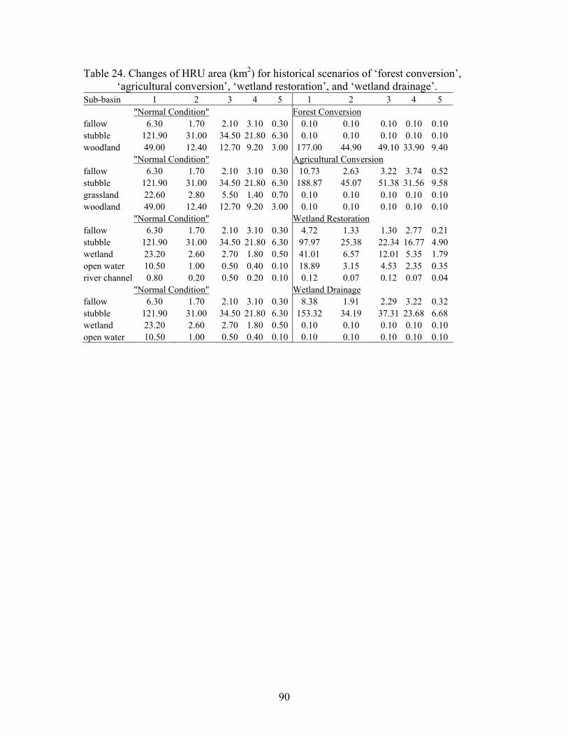
90
Table 24. Changes of HRU area (km2) for historical scenarios of ‘forest conversion’, ‘agricultural conversion’, ‘wetland restoration’, and ‘wetland drainage’.
Sub-basin 1 2 3 4 5 1 2 3 4 5 "Normal Condition" Forest Conversion fallow 6.30 1.70 2.10 3.10 0.30 0.10 0.10 0.10 0.10 0.10 stubble 121.90 31.00 34.50 21.80 6.30 0.10 0.10 0.10 0.10 0.10 woodland 49.00 12.40 12.70 9.20 3.00 177.00 44.90 49.10 33.90 9.40 "Normal Condition" Agricultural Conversion fallow 6.30 1.70 2.10 3.10 0.30 10.73 2.63 3.22 3.74 0.52 stubble 121.90 31.00 34.50 21.80 6.30 188.87 45.07 51.38 31.56 9.58 grassland 22.60 2.80 5.50 1.40 0.70 0.10 0.10 0.10 0.10 0.10 woodland 49.00 12.40 12.70 9.20 3.00 0.10 0.10 0.10 0.10 0.10 "Normal Condition" Wetland Restoration fallow 6.30 1.70 2.10 3.10 0.30 4.72 1.33 1.30 2.77 0.21 stubble 121.90 31.00 34.50 21.80 6.30 97.97 25.38 22.34 16.77 4.90 wetland 23.20 2.60 2.70 1.80 0.50 41.01 6.57 12.01 5.35 1.79 open water 10.50 1.00 0.50 0.40 0.10 18.89 3.15 4.53 2.35 0.35 river channel 0.80 0.20 0.50 0.20 0.10 0.12 0.07 0.12 0.07 0.04 "Normal Condition" Wetland Drainage fallow 6.30 1.70 2.10 3.10 0.30 8.38 1.91 2.29 3.22 0.32 stubble 121.90 31.00 34.50 21.80 6.30 153.32 34.19 37.31 23.68 6.68 wetland 23.20 2.60 2.70 1.80 0.50 0.10 0.10 0.10 0.10 0.10 open water 10.50 1.00 0.50 0.40 0.10 0.10 0.10 0.10 0.10 0.10

91
Table 25. Changes of routing distribution parameter between HRUs within the sub-basins for historical scenarios of ‘forest conversion’, ‘agricultural conversion’, ‘wetland restoration’, and ‘wetland drainage’.
HRU fallow stubble grassland river channel open water woodland wetland "Normal Condition" fallow 0 0 0 0.28 0.13 0.38 0.21 stubble 0 0 0 0.28 0.13 0.38 0.21 grassland 0 0 0 0.28 0.13 0.38 0.21 open water 0 0 0 1 0 0 0 woodland 0 0 0 0.45 0.21 0 0.34 wetland 0 0 0 0 1 0 0 river channel 0 0 0 0 0 0 0 Forest Conversion fallow 0 0 0 0.28 0.13 0.38 0.21 stubble 0 0 0 0.28 0.13 0.38 0.21 grassland 0 0 0 0.28 0.13 0.38 0.21 open water 0 0 0 1 0 0 0 woodland 0 0 0 0.45 0.21 0 0.34 wetland 0 0 0 0 1 0 0 river channel 0 0 0 0 0 0 0 Agricultural Conversion fallow 0 0 0 0.28 0.13 0.38 0.21 stubble 0 0 0 0.28 0.13 0.38 0.21 grassland 0 0 0 0.28 0.13 0.38 0.21 open water 0 0 0 1 0 0 0 woodland 0 0 0 0.45 0.21 0 0.34 wetland 0 0 0 0 1 0 0 river channel 0 0 0 0 0 0 0 Wetland Restoration fallow 0 0 0 0.07 0.24 0.31 0.38 stubble 0 0 0 0.07 0.24 0.31 0.38 grassland 0 0 0 0.07 0.24 0.31 0.38 open water 0 0 0 1 0 0 0 woodland 0 0 0 0.10 0.35 0 0.55 wetland 0 0 0 0 1 0 0 river channel 0 0 0 0 0 0 0 Wetland Drainage fallow 0 0 0 0.40 0.03 0.53 0.03 stubble 0 0 0 0.40 0.03 0.53 0.03 grassland 0 0 0 0.40 0.03 0.53 0.03 open water 0 0 0 1 0 0 0 woodland 0 0 0 0.86 0.07 0 0.07 wetland 0 0 0 0 1 0 0 river channel 0 0 0 0 0 0 0

92
7.2 Results of Scenario Simulations 7.2.1 2007-2008 Scenarios Simulations Results The results of 2007-2008 scenario simulations are shown in Figures 41 to 46. In each figure, there are five values corresponding to five levels of conversion at a stage; the ‘2007-08 normal case’ is indicated by the value at no conversion, and value at 100% of conversion implies the complete conversion, with other three values present at 25%, 50%, and 75%. The sensitivity of springtime discharge, total winter snow accumulation, blowing snow transport and sublimation, total infiltration, and springtime surface depression storage is assessed for the entire basin. There is a trend for springtime basin discharge to increase with increasing forest cover at both initial and mature stages, shown in Figure 41(a). Increases in spring discharge of 57% (initial stage) and 41% (mature stage) were estimated for complete conversion to forest cover. This is a very different result than is generated in many other parts of the world where increasing forest cover is associated with reduced runoff. The reason for this is that there is less loss to blowing snow sublimation (Figure 44(a)) and subsequently more snow accumulation in the forest (Figure 42(a)) even though both infiltration and springtime surface depression storage are increased as cropland is converted to woodland shown in Figure 45(a) and Figure 46(a). Smith Creek forests are deciduous and so have no winter interception losses in contrast to large interception losses associated with evergreen forests. The impact of increased snow accumulation in woodland on runoff outweighs the countering impact of increased infiltration and surface depression storage. For each level of conversion to woodland (25% to 100%), basin discharge at the initial stage is always greater than that at mature stage. The difference in discharge between two stages is mainly caused by differences in surface depression storage. The scenarios for conversion to ‘primarily agricultural land use’ show the reverse results compared to the scenarios of conversion to ‘complete forest cover’; that is, there is less discharge as a result of the conversion. For complete conversion to agricultural land use, there are decreases in spring discharge of 9% (initial stage) and 2% (mature stage). Interestingly, spring discharge shows a low sensitivity to various levels of conversion for ‘primarily agricultural land use’ (Figure 41(b)). Both infiltration (Figure 45(b)) and springtime surface depression storage (Figure 46(b)) decrease under conversion to cropland, but there is a greater decrease in winter snow accumulation (Figure 42(b)) due to enhanced blowing snow sublimation (Figure 44(b)) favoured by shorter plants. Compared to the initial stage of conversion, the basin discharge is higher at various levels of conversion at the mature stage shown in Figure 41(b). This is due to cropland possessing antecedent sdmax from grassland and woodland at the initial stage of conversion, which is higher than cropland’s own sdmax, whereas at the mature stage of conversion, cropland finally establishes its own sdmax. For scenarios of conversion to ‘high natural wetland extent/poorly drained’, the winter snow accumulation showed a small increase (Figure 42(c)) due to suppression of blowing snow sublimation by taller vegetation (Figure 44(c)). In addition, infiltration is reduced (Figure 45(c)), which favours more runoff, but there is more surface depressional storage

93
Smith Creek Springtime Basin Discharge
0
1
2
3
4
5
6
0 25 50 75 100
Percentage of Conversion (%)
Tota
l Bas
in D
ishc
arge
(100
0 da
m3 )
minimal wetland extent (initial stage)
minimall wetland extent (mature stage)
Smith Creek Springtime Basin Discharge
0
0.5
1
1.5
2
2.5
3
0 25 50 75 100
Percentage of Conversion (%)
Tota
l Bas
in D
ishc
arge
(100
0 da
m3 )
primarily agricultural land use (initial stage)
primarily agricultural land use (mature stage)
Smith Creek Springtime Basin Discharge
0
0.5
1
1.5
2
2.5
3
3.5
4
4.5
0 25 50 75 100
Percentage of Conversion (%)
Tota
l Bas
in D
ishc
arge
(100
0 da
m3 )
complete forest cover (initial stage)
complete forest cover (mature stage)
Smith Creek Springtime Basin Discharge
0
0.5
1
1.5
2
2.5
3
0 25 50 75 100
Percentage of Conversion (%)
Tota
l Bas
in D
ishc
arge
(100
0 da
m3 )
high natural wetland extent (initial stage)
high natural wetland extent (mature stage)
(a)
(c) (d)
(b)
Figure 41. Scenarios of Smith Creek 2008 springtime basin discharge: (a) ‘complete
forest cover’, (b) ‘primarily agricultural land use’, (c) ‘high natural wetland extent/poorly drained’, and (d) ‘minimal wetland extent/well drained’.
Total Winter Snow Accumulation at Smith Creek Basin
91
92
93
94
95
96
97
98
99
100
101
0 25 50 75 100
Percentage of Conversion (%)
Tota
l Bas
in S
now
Acc
umul
atio
n (m
m S
WE)
complete forest cover (initial stage)
complete forest cover (mature stage)
Total Winter Snow Accumulation at Smith Creek Basin
91.8
92
92.2
92.4
92.6
92.8
93
93.2
93.4
93.6
93.8
0 25 50 75 100
Percentage of Conversion (%)
Tota
l Bas
in S
now
Acc
umul
atio
n (m
m S
WE)
high natural wetland extent (initial stage)
high natural wetland extent (mature stage)
(a)
(c) Total Winter Snow Accumulation at Smith Creek Basin
86
87
88
89
90
91
92
93
0 25 50 75 100
Percentage of Conversion (%)
Tota
l Bas
in S
now
Acc
umul
atio
n (m
m S
WE)
minimal wetland extent (initial stage)
minimal wetland extent (mature stage)
Total Winter Snow Accumulation at Smith Creek Basin
86
87
88
89
90
91
92
93
0 25 50 75 100
Percentage of Conversion (%)
Tota
l Bas
in S
now
Acc
umul
atio
n (m
m S
WE)
primarily agricultural land use (initial stage)
primarily agricultural land use (mature stage)
(b)
(d)
Figure 42. Scenarios of total winter 2007-2008 snow accumulation at Smith Creek basin:
(a) ‘complete forest cover’, (b) ‘primarily agricultural land use’, (c) ‘high natural wetland extent/poorly drained’, and (d) ‘minimal wetland extent/well drained’.

94
Total Blowing Snow Transport at Smith Creek Basin
0
0.01
0.02
0.03
0.04
0.05
0.06
0.07
0 25 50 75 100
Percentage of Conversion (%)
Tota
l Bas
in B
low
ing
Snow
Tr
ansp
ort (
mm
SW
E)
high natural wetland extent (initial stage)
high natural wetland extent (mature stage)
Total Blowing Snow Transport at Smith Creek Basin
0
0.01
0.02
0.03
0.04
0.05
0.06
0.07
0 25 50 75 100
Percentage of Conversion (%)
Tota
l Bas
in B
low
ing
Snow
Tr
ansp
ort (
mm
SW
E)
complete forest cover (initial stage)
complete forest cover (mature stage)
(a)
(c)
Total Blowing Snow Transport at Smith Creek Basin
0
0.01
0.02
0.03
0.04
0.05
0.06
0.07
0.08
0.09
0.1
0 25 50 75 100
Percentage of Conversion (%)
Tota
l Bas
in B
low
ing
Snow
Tr
ansp
ort (
mm
SW
E)
primarily agricultural land use (initial stage)
primarily agricultural land use (mature stage)
(b)
Total Blowing Snow Transport at Smith Creek Basin
0.061
0.062
0.063
0.064
0.065
0.066
0.067
0.068
0.069
0 25 50 75 100
Percentage of Conversion (%)To
tal B
asin
Blo
win
g Sn
ow
Tran
spor
t (m
m S
WE)
minimal wetland extent (initial stage)
minimal wetland extent (mature stage)
(d)
Figure 43. Scenarios of 2007-2008 seasonal blowing snow transport at Smith Creek basin:
(a) ‘complete forest cover’, (b) ‘primarily agricultural land use’, (c) ‘high natural wetland extent/poorly drained’, and (d) ‘minimal wetland extent/well drained’.
Total Blowing Snow Sublimation at Smith Creek Basin
0
1
2
3
4
5
6
7
8
9
0 25 50 75 100
Percentage of Conversion (%)
Tota
l Bas
in B
low
ing
Snow
Su
blim
atio
n (m
m S
WE)
high natural wetland extent (initial stage)
high natural wetland extent (mature stage)
Total Blowing Snow Sublimation at Smith Creek Basin
0
1
2
3
4
5
6
7
8
9
0 25 50 75 100
Percentage of Conversion (%)
Tota
l Bas
in B
low
ing
Snow
Su
blim
atio
n (m
m S
WE)
complete forest cover (initial stage)
complete forest cover (mature stage)
(a)
(c)
Total Blowing Snow Sublimation at Smith Creek Basin
0
2
4
6
8
10
12
14
0 25 50 75 100
Percentage of Conversion (%)
Tota
l Bas
in B
low
ing
Snow
Su
blim
atio
n (m
m S
WE)
primarily agricultural land user (initial stage)
primarily agricultural land use (mature stage)
(b)
Total Blowing Snow Sublimation at Smith Creek Basin
8.4
8.6
8.8
9
9.2
9.4
9.6
0 25 50 75 100
Percentage of Conversion (%)
Tota
l Bas
in B
low
ing
Snow
Su
blim
atio
n (m
m S
WE)
minimal wetland extent (initial stage)
minimal wetland extent (mature stage)
(d)
Figure 44. Scenarios of 2007-2008 seasonal blowing snow sublimation at Smith Creek: (a)
‘complete forest cover’, (b) ‘primarily agricultural land use’, (c) ‘high natural wetland extent/poorly drained’, and (d) ‘minimal wetland extent/well drained’.

95
Total Infiltration at Smith Creek Basin
31
31.5
32
32.5
33
33.5
34
34.5
35
35.5
36
0 25 50 75 100
Percentage of Conversion (%)
Tota
l Bas
in In
filtra
tion
(mm
SW
E)
complete forest cover (initial stage)
complete forest cover (mature stage)
Total Infiltration at Smith Creek Basin
30
30.2
30.4
30.6
30.8
31
31.2
31.4
31.6
31.8
0 25 50 75 100
Percentage of Conversion (% )
Tota
l Bas
in In
filtr
atio
n (m
m
SWE)
primarily agricultural land use (initial stage)
primarily agricultural land use (mature stage)
Total Infiltration at Smith Creek Basin
29
29.5
30
30.5
31
31.5
32
0 25 50 75 100
Percentage of Conversion (% )
Tota
l Bas
in In
filtra
tion
(mm
S
WE
)
high natural wetland extent (initial stage)
high natural wetland extent (mature stage)
Total Infiltration at Smith Creek Basin
31.2
31.4
31.6
31.8
32
32.2
32.4
32.6
32.8
0 25 50 75 100
Percentage of Conversion (% )To
tal B
asin
Infil
tratio
n (m
m
SW
E)
minimal wetland extent (initial stage)
minimal wetland extent (mature stage)
(a)
(d)(c)
(b)
Figure 45. Scenarios of 2008 spring (total) infiltration at Smith Creek basin: (a)
‘complete forest cover’, (b) ‘primarily agricultural land use’, (c) ‘high natural wetland extent/poorly drained’, and (d) ‘minimal wetland extent/well drained’.
Total Springtime Surface Depression Storage at Smith Creek Basin
55.5
56
56.5
57
57.5
58
58.5
0 25 50 75 100
Percentage of Conversion (% )
Tota
l Spr
ingt
ime
Surfa
ce
Dep
ress
ion
Sto
rage
(mm
SW
E) complete forest cover (initia l stage)
complete forest cover (mature stage)
Total Springtime Surface Depression Storage at Smith Creek Basin
54.5
55
55.5
56
56.5
57
0 25 50 75 100
Percentage of Conversion (% )
Tota
l Spr
ingt
ime
Surfa
ce
Dep
ress
ion
Sto
rage
(mm
SW
E)
primarily agricultural land use (initial stage)
primarily agricultural land use (mature stage)
Total Springtime Surface Depression Storage at Smith Creek Basin
0
10
20
30
40
50
60
70
0 25 50 75 100
Percentage of Conversion (% )
Tota
l Spr
ingt
ime
Surfa
ce
Dep
ress
ion
Sto
rage
(mm
SW
E)
high natural wetland extent (initia l stage)
high natural wetland extent (mature stage)
Total Springtime Surface Depression Storage at Smith Creek Basin
0
10
20
30
40
50
60
0 25 50 75 100
Percentage of Conversion (% )
Tota
l Spr
ingt
ime
Surfa
ce
Dep
ress
ion
Sto
rage
(mm
SW
E)
minimal wetland extent (initia l stage)
minimal wetland extent (mature stage)
(a)
(d)(c)
(b)
Figure 46. Scenarios of 2008 springtime surface depression storage at Smith Creek basin:
(a) ‘complete forest cover’, (b) ‘primarily agricultural land use’, (c) ‘high natural wetland extent/poorly drained’, and (d) ‘minimal wetland extent/well drained’.
96
to hold the runoff, especially for the conversion at the mature stage shown in Figure 46(c). These factors counterbalance each other somewhat resulting in spring basin discharge dropping by 79% at the mature stage (Figure 41(c)). On the other hand, spring basin discharge shows a high sensitivity for scenarios of conversion to ‘minimal wetland extent/well drained’ (Figure 41(d)). Although when converting wetland/open water to cropland the basin accumulates less snow (Figure 42(d)), because of greater sublimation losses (Figure 44(d)), the loss of surface depression storage capacity overwhelms the effect of decreasing snow accumulation on runoff generation. Consequently, far more discharge is generated for the basin – an increase of 117% in spring discharge at the mature stage is estimated for complete wetland drainage in the basin. Woodland and grassland cover about 119 km2 at Smith Creek basin (~393 km2) and wetland and open water cover about 43 km2. The fall soil moisture contents for woodland and grassland were very similar to cropland, whereas wetland and open water have much higher values. In addition, sdmax for wetland/open water is much higher than that for cropland, woodland or grassland. Hence, changing wetland/open water conditions causes a much larger impact on cumulative spring basin discharge than does altering woodland/grassland conditions, even though these latter HRUs cover relatively small areas of the basin. 7.2.2 Historical Scenarios Simulations Results i. Cumulative Spring Discharge The scenario simulation results of cumulative spring discharge in Smith Creek during the 29-year period: 1965-82 and 1993-2005 are shown in Figure 47. Keep in mind that the cumulative spring discharge under “normal condition” is only a simulated hypothetical basin discharge using the current land use fixed from year to year with the historical meteorology, and initial (fall) conditions recorded during the 29-year period. Since land use and drainage have changed over 29 years the “normal condition” did not actually occur consistently over this period of time, it is only used as a reference point for evaluating the hydrological changes due to land use and drainage. Figure 47 shows the cumulative spring discharge for Smith Creek under various scenarios, ranging from land use scenarios (i.e. forest conversion versus agricultural conversion) to drainage scenarios (i.e. wetland restoration versus wetland drainage). The figure also demonstrates the variable changes of discharge not only in high flow years, but also in low flow and medium flow years. Results for the sensitivity of total basin spring discharge to changes in land use and drainage are shown in Figure 48, which plots the changes in discharge in comparison to discharge. For the forest conversion scenario shown in Figure 48(a), there is a variable effect on the cumulative spring discharge, which can either increase or decrease dramatically for low to moderate flows (total spring discharge between 0 and 10,000 dam3). However there is a slight trend for cumulative spring discharge to decrease upon forest conversion for moderate to high flows. For agricultural conversion, similar to the

97
forest conversion scenario, there is a variable effect on the cumulative spring discharge for the low flows, but the total spring discharge increases for moderate and high flows (Figure 48(b)). Cumulative spring discharge shows very dramatic changes for the drainage scenario in comparison to smaller changes associated with agricultural or forest land use conversion. That is, the total spring discharge decreases with wetland restoration (Figure 48(c)) and increases with wetland drainage (Figure 48(d)). The greatest impact for both scenarios occurs for moderate spring discharges (around 10,000 dam3) for which the spring discharge drops by 6,000 to 8,000 dam3 when restoring wetland storage and reducing channel drainage and rises by 3,000 to 8,000 dam3 when increasing channel drainage and removing wetland storage. Changes moderate for higher flow seasons, likely due to limitations of available storage changes in response to drainage changes. Overall, the long-term impact of land use and drainage change during the 29-year period (1965-82 and 1993-2005) on the Smith Creek cumulative spring discharge is shown in Figure 49. The basin spring streamflow is most sensitive to changes in wetland storage and channel drainage condition; there would be an average decrease for restoring wetland and an average increase for draining wetland by more than 2,000 dam3 during this long-term period. This leads to a 45% drop in the total basin spring discharge for wetland restoration and a 36% rise for wetland drainage. For the same period, there would be a very small effect (an average 1% increase) on the basin spring discharge from converting cropland to forest and a moderate increase (19% increase) for conversion of woodland to agricultural land use (Figure 49). ii. Peak Daily Discharge Peak daily spring discharge in Smith Creek during 29 year periods: 1965-82 and 1993-2005 was simulated for various land use and drainage scenarios is shown in Figure 50. During this 29 year periods, the peak daily discharge in spring tends to increase for forest conversion, agricultural conversion, and wetland drainage scenarios and decreases for the wetland restoration scenario. The reason for the increases in the peak discharge when converting cropland to forest is that the hydrograph under this conversion tends to become sharper and less attenuated. In other words, the spring hydrograph develops a shorter duration and higher peak. Both the agricultural conversion and wetland drainage, tend to increase the total spring discharge volume, which leads to higher peak discharge. Conversely, wetland restoration results in reduced peak spring discharge due to increased wetland capacity for storing runoff and subsequent decreasing the seasonal discharge volume.

98
Scenarios of Smith Creek Cumulative Spring Discharge
05
1015202530354045
1965
-6619
66-67
1967
-6819
68-69
1969
-7019
70-71
1971
-7219
72-73
1973
-7419
74-75
1975
-7619
76-77
1977
-7819
78-79
1979
-8019
80-81
1981
-8219
93-94
1994
-9519
95-96
1996
-9719
97-98
1998
-9919
99-20
0020
00-01
2001
-0220
02-03
2003
-0420
04-05
Sprin
g D
isch
arge
(100
0 da
m3 ) "Normal Condition"
Forest ConversionAgricultural ConversionWetland RestorationWetland Drainage
Figure 47. Simulations of scenarios of Smith Creek cumulative spring discharge during 1965-82 and 1993-2005 periods.

99
Wetland Restoration Scenario
-9-8-7-6-5-4-3-2-101
0 5 10 15 20 25 30 35 40 45
Cumulative Spring Discharge (1000 dam3)
Chan
ge in
Dis
char
ge
Vol
ume
(100
0 da
m3 )
Wetland Drainage Scenario
0123456789
0 5 10 15 20 25 30 35 40 45
Cumulative Spring Discharge (1000 dam3)
Chan
ge in
Dis
char
ge
Vol
ume
(100
0 da
m3 )
Forest Conversion Scenario
-4
-2
0
2
4
6
8
0 5 10 15 20 25 30 35 40 45
Cumulative Spring Discharge (1000 dam3)
Cha
nge
in D
isch
arge
Vo
lum
e (1
000
dam
3 )
Agricultural Conversion Scenario
-3-2-1012345
0 5 10 15 20 25 30 35 40 45
Cumulative Spring Discharge (1000 dam3)
Cha
nge
in D
isch
arge
Vo
lum
e (1
000
dam
3 )
(a) (b)
(c) (d)
Figure 48. Sensitivity of the Smith Creek cumulative spring discharge during 1965-82 and 1993-2005 periods: (a) forest conversion scenario, (b) agricultural conversion scenario, (c) wetland restoration scenario, and (d) wetland drainage scenario.

100
Long-term Impact of Land Use and Drainage Change(1965-82 & 1993-2005)
-4
-3
-2
-1
0
1
2
3
Forest Conversion AgriculturalConversion
Wetland Restoration Wetland Drainage
Cha
nge
in D
isch
arge
Vol
ume
(100
0 da
m3 )
Figure 49. Effect of long-term land use and drainage change on Smith Creek cumulative
spring discharge. Results for the sensitivity of peak daily spring discharge to changes in land use and drainage are shown in Figure 51. The figure shows the effects on land use and drainage change on the peak daily discharge for a variety of seasonal discharge volumes. There is a variable effect on the peak daily discharge for low flows, (spring discharge volume between 0 and 10,000 dam3) when converting all cropland to forest cover. There are some drops but predominately increases in peak daily discharge for the low flow conditions (Figure 51(a)). The peak daily discharge increases sharply on conversion to forest to cropland for moderate and high flows (spring discharge volume > 10,000 dam3), with the highest impact occurring for the highest measured spring discharge volume. This is likely due to the forest cover synchronizing melt runoff compared to the mixed open landscapes. When converting to cropland, a variable effect on the peak daily discharge is found for the low flow seasons (Figure 51(b)). There were some decreases in the peak discharge but majority showed an increase. Figure 51(b) also showed a variable effect of agricultural conversion on the peak discharge for moderate flows with some increases and some decreases; the greatest impact occurring for the spring discharge around 15,000 dam3, with smaller impacts for high flows. In the drainage scenario shown in Figure 51(c) and (d), restoring wetland and draining wetland tended to effectively reduce and raise the peak daily discharge for the low flow, respectively. Effects of restoring wetland and reducing channel drainage on decreasing the peak discharge are overwhelmed for the moderate and high flows (Figure 51(c)). Interestingly, removing wetland and increasing channel drainage reduced the peak daily discharge for the moderate flow (Figure 51(d)), which is counterintuitive. This is attributed to the fact that the length of channel increases and consequently takes longer time for streamflow to travel to the basin outlet, and the hydrograph becomes more attenuated. Drainage has similar effects on the peak discharge, a 1.6 m3 s-1 increase. The wetland restoration on average contributes to a decrease in the peak discharge by about 2.6 m3 s-1.

101
Scenarios of Smith Creek Peak Daily Spring Discharge
0
10
20
30
40
50
60
1965
-6619
66-67
1967
-6819
68-69
1969
-7019
70-71
1971
-7219
72-73
1973
-7419
74-75
1975
-7619
76-77
1977
-7819
78-79
1979
-8019
80-81
1981
-8219
93-94
1994
-9519
95-96
1996
-9719
97-98
1998
-9919
99-20
0020
00-01
2001
-0220
02-03
2003
-0420
04-05
Peak
Dai
ly D
isch
arge
(m3 /s
) "Normal Condition"Forest ConversionAgricultural ConversionWetland RestorationWetland Drainage
Figure 50. Simulations of scenarios of Smith Creek peak daily spring discharge during 1965-82 and 1993-2005 periods.

102
Wetland Drainage Scenario
-4
-2
0
2
4
6
0 5 10 15 20 25 30 35 40 45
Cumulative Spring Discharge (1000 dam3)
Cha
nge
in P
eak
Daily
Di
scha
rge
(m3 /s
)
Wetland Restoration Scenario
-12-10-8-6-4-20246
0 5 10 15 20 25 30 35 40 45
Cumulative Spring Discharge (1000 dam3)
Chan
ge in
Pea
k D
aily
D
isch
arge
(m3 /s
)
Agricultural Conversion Scenario
-4
-2
0
2
4
6
8
10
0 5 10 15 20 25 30 35 40 45
Cumulative Spring Discharge (1000 dam3)
Cha
nge
in P
eak
Daily
Di
scha
rge
(m3 /s
)
Forest Conversion Scenario
-5
0
5
10
15
20
25
30
0 5 10 15 20 25 30 35 40 45
Cumulative Spring Discharge (1000 dam3)
Chan
ge in
Pea
k D
aily
D
isch
arge
(m3 /s
)
(a) (b)
(c) (d)
Figure 51. Sensitivity of the Smith Creek peak daily spring discharge during 1965-82 and 1993-2005 periods: (a) forest conversion
scenario, (b) agricultural conversion scenario, (c) wetland restoration scenario, and (d) wetland drainage scenario.

103
Long-term Impact of Land Use and Drainage Change(1965-82 & 1993-2005)
-3
-2
-1
0
1
2
3
4
Forest Conversion AgriculturalConversion
Wetland Restoration Wetland Drainage
Cha
nge
in P
eak
Dai
ly D
isch
arge
(m3 /s
)
Figure 52. Effect of long-term land use and drainage change on Smith Creek peak daily
spring discharge. Overall, the long-term impact of land use and drainage change during the 29-year period (1965-82 and 1993-2005) on the Smith Creek peak daily spring discharge is shown in Figure 52. The forest conversion, agricultural conversion, and wetland drainage scenarios all lead to higher peak daily discharge, whereas wetland restoration contributes to reducing the peak discharge. During this long-term period, forest conversion has the highest increase in the peak discharge, by about 3.5 m3 s-1, and both agricultural conversion and wetland land use scenarios are equally important in affecting the basin peak daily spring discharge compared to drainage scenarios shown in Figure 52. It should be noted that the complex response of peak discharge to drainage and restoration shown in Fig. 51 requires that substantial caution be exercised in interpreting Fig. 52.

104
8. Conclusions and Recommendations 8.1 Conclusions The Canadian Prairie pothole region is characterized by numerous post-glacial surface depressions. These surface depressions form wetlands which are an important factor in controlling streamflow generation and the water balance. The ability of wetlands to trap blowing snow in winter and store runoff water is crucial to hydrological cycling on the Prairies, and has posed a substantial challenge to hydrological modelling. A Prairie Hydrological Model (PHM) was developed by adding a new module in the Cold Regions Hydrological Model platform (CRHM) to deal with wetland water storage. Both the calibrated (based on the photogrammetric based DEM) and uncalibrated (based on the LiDAR derived DEM) modelling approaches were involved in model parameterization and were used to predict water balance in the Smith Creek Research Basin, Saskatchewan. Both calibrated and uncalibrated predictions of winter snow accumulation were very similar and compared quite well with many of the distributed field observations. The simulations were able to effectively capture the prairie blowing snow sequence (Fang and Pomeroy, 2009) and relocate snow from ‘source’ areas (e.g. fallow and stubble fields) to ‘sink’ or ‘drift’ areas (e.g. tall vegetated wetland area and deeply incised channels). This is a vital process in governing the water balance of prairie basins as the majority of water in wetlands and prairie river channels has been shown previously to be the result of redistribution of snow by wind (Fang and Pomeroy, 2008; 2009) and subsequent snowmelt runoff. However, poorer streamflow predictions were noticed for the 2009 melt period. The 12.6 mm rainfall on 22 March 2009 was followed by days with high incoming solar radiation but no substantial snowmelt. The PHM albedo module reduced the albedo in response to the rainfall event resulting in rapid snowmelt and runoff generation over the post rainfall sunny period - well ahead of actual melt and runoff generation. A delay start for melt was imposed in the PHM energy-budget snowmelt module to match the onset of snowmelt. Rainfall events such as the one on 22 March 2009 are rare in the prairie environment during early spring (Male and Gray, 1981) and have been seldom studied. Fang and Pomeroy (2007) suggested that they will become more common under climate warming scenarios predicted for Saskatchewan in the mid-21st century. Therefore, further investigations of snow albedo dynamics in the early spring rainfall events are needed. Soil moisture status is also an important factor in determining the spring surface runoff (Gray et al., 1985; Zhao and Gray, 1997) and is crucial for agricultural production. Soil moisture content at a point during early spring was adequately simulated from both modelling approaches but could not be verified for the whole basin. No difference between the two modelling approaches was found because both approaches used the same method for predicting soil moisture status.
105
Both modelling approaches were capable of matching the streamflow hydrographs with good accuracy in the 2008 simulation period; the calibrated approach performed slightly better than the uncalibrated approach because the depressional storage was calibrated to optimise the streamflow hydrograph, whereas no calibration was involved in the uncalibrated simulation. The estimated parameters were kept the same for both calibrated and uncalibrated simulations in the 2009 simulation period, where the hydrographs produced had a generally similar shape to observed one, but were of lower magnitude. Seasonal discharge volumes were underestimated. The hydrograph simulations in 2009 were largely affected by uncertainty of the rain on snow modelling mentioned above and model’s single wetland HRU representation for the entire basin. An additional test on the model performance in predicting Smith Creek spring streamflow using Yorkton meteorology indicates that having meteorology information from within the basin is quite important to accuracy of basin water balance predictions. The uncalibrated modelling approach utilized LiDAR DEM, SPOT 5 satellite images, stream networks and wetland inventory GIS data and involved automated basin parameters delineation techniques and simplified wetland depth-area-volume calculation. This process can be regarded as a model parameterization procedure. Through this process, basin physiographic parameters such as basin area and elevation and important hydrological process parameters such as blowing snow fetch distance, wetland surface depression storage, and surface runoff and channel flow routing parameters were derived successfully. Although the calibrated modelling approach can produce better hydrograph matching, its applicability to other basins is restricted by the nature of calibration and difficulties in regionalizing depressional storage values that substantially deviate from true values and are a characteristic of local topography. On the other hand, the uncalibrated parameterization process did not rely on parameter calibration, suggesting that this whole pre-modelling parameterization method can be applied to other prairie basins as long as detailed meteorology, basin land use, and physiography data are available. It is expected that these will be available in the near future for much of the Prairies. The simplified LiDAR V-A-h method was developed to derive wetland characteristics. While total wetland depth cannot be measured directly from the LiDAR DEM, multiple area measurements and the change in depth between them can be extracted through a simple GIS analysis of the DEM. If a constant p value is assumed, the total depth of the wetland, and thus the s coefficient can be estimated and used in the simplified V-A-h method to estimate volume. Estimations of Vmax made with these data outperformed estimates generated with the V-A equations (Wiens, 2001; Gleason et al., 2007). This was likely due to the inclusion of information on depression morphology when calculating volume. Further, the process to retrieve the coefficients from a LiDAR DEM was automated and wetland storage was estimated at a broad spatial scale. A GIS model and Visual Basic script were created that can automatically extract the elevation and area data necessary for use in the simplified V-A-h method. Although the model still requires user input such as the minimum area to retain and the p coefficient, the process to retrieve the data is quite fast and allows for a large area to be analyzed in a short period of time. The

106
SDNWA case study illustrated that the LiDAR V-A-h method can be applied to a small prairie watershed to accurately predict wetland water storage. Using the Prairie Hydrological Model, PHM, a series of scenarios on changing land use and wetland and drainage conditions was created from 2007-08 meteorological data. The scenario simulations were used to calculate cumulative spring basin discharge, total winter snow accumulation, blowing snow transport and sublimation, cumulative infiltration, and spring surface depression storage status. The results showed these processes were sensitive to the land use change and to altering wetland and drainage conditions. From these simulations, spring streamflow decreased by 2% with complete conversion to agriculture and 79% with complete restoration of wetlands; conversely it increased 41% with complete conversion to forest cover and by 117% with complete wetland drainage. Wetland changes had a stronger effect on discharge volumes than land use changes. The greatest sensitivity was to further drainage of wetlands which substantially increased streamflow. An additional sensitivity analysis of the effect of various scenarios on basin streamflow using historical (i.e. 29-year periods: 1965-82 and 1993-2005) meteorology, fall conditions was carried out with current land use and drainage as the reference condition. Results showed that the effects of land use change and wetland drainage alteration on cumulative basin spring discharge volume and peak daily spring discharge were highly variable from year to year and depended on the spring discharge volume. Both land use scenarios: forest conversion and agricultural conversion increased peak discharge. In contrast wetland restoration and wetland drainage scenarios reduced and raised peak discharge, respectively. However there was considerable variation in these relationships with opposing behaviour found for moderate discharge volume seasons. Forest conversion and agricultural conversion increased the long-term average spring discharge volume by small amounts: 1% and 19%, respectively. Larger impacts were found from drainage alteration scenarios. That is, restoring wetlands reduced spring discharge volumes by 45%, and draining wetlands caused a 36% increase. The differences between these long term averages and the 2007-2008 reference year shows the importance of long term investigation of basin response to land use and drainage changes.

107
8.2 Recommendations Recommendation 1: To model a prairie basin with substantial wetland drainage development, a greater variety of wetland representations are needed and these need to include both hydraulic and hydrological characteristics of wetlands. That is, a model should not only have ‘intact wetland’ representation, but also include ‘drained wetland’ representations. Drained wetlands do not display fill and spill behaviour but have linear reservoir characteristics that will require specification of stage-outflow relationships. In the ‘drained wetland’, several sub-classes should be made to differentiate the hydraulic characteristics of newly drained wetlands from established drained wetland. It is anticipated that including more wetland classes in the model would improve the prediction for the cumulative volume of basin discharge and for hydrograph recession curves. Consideration of the hydraulic behaviour of drained wetlands might also provide an additional wetland management tool. Recommendation 2: It is important and imperative to collect meteorology information within or very near to a basin to have a reasonable prediction of water balance in the prairie environment. This is problematic given the sparse meteorological measurement network in Saskatchewan. Recommendation 3: The benefits derived from using a LiDAR derived DEM in prairie hydrological modelling are high. Canadian prairie basins are characterized by many depressions; using a conventional low quality DEM (even photogrammetrically derived) would not be accurate enough to produce prairie channel networks or estimate the basin area. Therefore, a LiDAR derived DEM is highly recommended for hydrological modelling in prairie basins. Applying various automated GIS tools with LiDAR DEM can generate reasonable channel networks and quantify basin surface depressional storage. There is no other way to confidently quantify wetland depressional storage in the Prairie environment and this quantification is crucial to estimating stream hydrology. Recommendation 4: At Smith Creek, wetland restoration and drainage appear to have stronger controls on stream discharge volume than do land use changes, but land use changes have stronger controls on peak discharge. This conclusion has strong policy implications but has been determined for only one basin in the Prairies. Basins in other parts of the Prairies with differing wetland configurations, drainage, soils, vegetation and climate should be investigated to see if this is a general conclusion or one that is specific to the region around Smith Creek.

108
List of References Agriculture and Agri-Food Canada. 1998. Drought in the Palliser Triangle.
PFRA Publications. Retrieved: March 20, 2007. [Web Page]. Available at: http://www.agr.gc.ca/pfra/publications_e.htm.
Annandale, J.G., Jovanovic, N.Z., Benadé, N. and Allen, R.G. 2002. Software for missing data error analysis of Penman-Monteith reference evapotranspiration. Irrigation Science 21: 57-67.
Bagnold, R.A. 1954. The Physics of Blown Sand and Desert Dunes. Chapman & Hall: London, 265.
Berthold, S., Bentley, L.R. and Hayashi, M. 2004. Integrated hydrogeological and geophysical study of depression-focused groundwater recharge in the Canadian prairies. Water Resources Research 40: W06505.
Bodhinayake, W. and Si, B.C. 2004. Near-saturated surface soil hydraulic properties under different land uses in the St Denis National Wildlife Area, Saskatchewan, Canada. Hydrological Processes 18: 2835-2850.
Chow, V.T. 1959. Open Channel Hydraulics. McGraw-Hill, Inc. New York, USA. Chow, V.T. 1964. Handbook of Applied Hydrology. McGraw-Hill, Inc. New York, USA. Dornes, P.F., Pomeroy, J.W., Pietroniro, A., Carey, S.K. and Quinton, W.L. 2008.
Influence of landscape aggregation in modelling snow-cover ablation and snowmelt runoff in a sub-arctic mountainous environment. Hydrological Sciences Journal, 53(4), 725-740.
Dyck, G.E. and Gray, D.M. 1976. Investigation of the areal variability within the Bad Lake Watershed, Saskatchewan. 1975/76 Final Report. Division of Hydrology, University of Saskatchewan, Saskatoon. 32 pp.
Elliott, J.A. and Efetha, A.A. 1999. Influence of tillage and cropping system on soil organic matter, structure and infiltration in a rolling landscape. Canadian Journal of Soil Science 79: 457–463.
Environment Canada. 2009. Canadian climate normals 1971-2000. Retrieved: September 10, 2009. [Web Page]. Available at: http://www.climate.weatheroffice.ec.gc.ca/climate_normals/index_e.html.
Fang, X. and Pomeroy, J.W. 2007. Snowmelt runoff sensitivity analysis to drought on the Canadian Prairies. Hydrological Processes 21: 2594-2609.
Fang, X. and Pomeroy, J. W. 2008. Drought impacts on Canadian prairie wetland snow Hydrology. Hydrological Processes 22: 2858-2873.
Fang, X. and Pomeroy, J.W. 2009. Modelling blowing snow redistribution to prairie wetlands. Hydrological Processes 23: 2557-2569.
Garbrecht, J. and Martz, L.W. 1993. Network and subwatershed parameters extracted from digital elevation models: The Bills Creek experience. Water Resource Bulletin 29: 909-916.
Garbrecht, J. and Martz, L.W. 1997. The assignment of drainage direction over flat surfaces in raster digital elevation models. Journal of Hydrology 193: 204-213.
Garnier, B.J. and Ohmura, A. 1970. The evaluation of surface variations in solar radiation income. Solar Energy 13: 21-34.
Gleason, R.A., Tangen, B.A., Laubhan, M.K., Kermes, K.E. and Euliss, N.H. 2007.

109
Estimating water storage capacity of existing and potentially restorable wetland depressions in a subbasin of the Red river of the north. U.S. Geological Survey, U.S. Department of the Interior Open-file report 2007-1159.
Godwin, R.B. and Martin, F.R.J. 1975. Calculation of gross and effective drainage areas for the Prairie Provinces. In: Canadian Hydrology Symposium - 1975 Proceedings, 11-14 August 1975, Winnipeg, Manitoba. Associate Committee on Hydrology, National Research Council of Canada, pp. 219-223.
Granger, R.J., Chanasyk, D.S., Male, D.H. and Norum, D.I. 1977. Thermal regime of prairie snowcover. Soil Science Society of America Journal 41: 839-842.
Granger, R.J., Gray, D.M. and Dyck, G.E. 1984. Snowmelt infiltration to frozen Prairie soils. Canadian Journal of Earth Science 21: 669-677.
Granger, R.J. and Gray, D.M. 1989. Evaporation from natural non-saturated surfaces. Journal of Hydrology 111: 21–29.
Granger, R.J. and Gray, D.M. 1990. A net radiation model for calculating daily snowmelt in open environments. Nordic Hydrology 21: 217-234.
Granger, R.J., Pomeroy, J.W. and Parviainen, J. 2002. Boundary-layer integration approach to advection of sensible heat to a patchy snow cover. Hydrological Processes 16: 3559-3569.
Gray, D.M. 1970. Handbook on the Principles of Hydrology: with special emphasis directed to Canadian conditions in the discussions, applications and presentation of data. New York: Water Information Center, Inc..
Gray, D.M., Landine, P.G. and Granger, R.J. 1985. Simulating infiltration into frozen Prairie soils in stream flow models. Canadian Journal of Earth Science 22: 464-474.
Gray, D.M., Granger, R.J. and Landine, P.G. 1986. Modelling snowmelt infiltration and runoff in a prairie environment. In Kane, D.L. (Ed.), Proceedings of the Symposium: Cold Regions Hydrology. Maryland: American Water Resources Association, pp. 427-438.
Gray, D.M. and Landine, P.G. 1987. Albedo model for shallow prairie snow covers. Canadian Journal of Earth Sciences 24: 1760-1768.
Gray, D.M. and Landine, P.G. 1988. An energy-budget snowmelt model for the Canadian Prairies. Canadian Journal of Earth Sciences 25: 1292-1303.
Gray, D.M., Toth, B., Zhao, L., Pomeroy, J.W. and Granger, R.J. 2001. Estimating areal snowmelt infiltration into frozen soils. Hydrological Processes 15: 3095-3111.
Green, W.H. and Ampt, G.A. 1911. Studies on soil physics: 1. Flow of air and water through soils. Journal of Agricultural Science 4: 1-24.
Hack, J.T. 1957. Studies of longitudinal stream profiles in Virginia and Maryland. US Geological Survey Professional Paper, 294-B.
Hansen, B. 2000. Estimation of surface runoff and water-covered area during filling of surface microrelief depressions. Hydrological Processes 14: 1235-1243.
Hayashi, M., van der Kamp, G. and Rudolph, D.L. 1998. Water and solute transfer between a prairie wetland and adjacent uplands, 1. Water balance. Journal of Hydrology 207: 42-55.
Hayashi, M. and van der Kamp, G. 2000. Simple equations to represent the volume-area-depth relations of shallow wetlands in small topographic depressions. Journal of Hydrology 237: 74-85.

110
Hayashi, M., van der Kamp, G. and Schmidt, R. 2003. Focused infiltration of snowmelt water in partially frozen soil under small depressions. Journal of Hydrology 270: 214-229.
Kane, D.L. and Stein, J. 1983. Water movement into seasonally frozen soils. Water Resource Research 19: 1547-1557.
LaBaugh, J.W., Winter, T.C. and Rosenberry, D.O. 1998. Hydrologic functions of prairie wetlands, Great Plains Research 8, 17-37.
Lapen, D.R. and Martz, L.W. 1993. The measurement of two simple topographic indices of wind sheltering exposure from raster digital elevation models. Computer & Geosciences 19: 769-779.
Lapen, D.R. and Martz, L.W. 1996. An investigation of the spatial association between snow depth and topography in a Prairie agricultural landscape using digital terrain analysis. Journal of Hydrology 184: 277-298.
Leavesley, G.H., Lichty, R.W., Troutman, B.M. and Saindon, L.G. 1983. Precipitation-runoff modelling system: user’s manual. US Geological Survey Water Resources Investigations Report 83-4238. 207 pp.
Li, L. and Pomeroy, J.W. 1997a. Estimates of threshold wind speed for snow transport using meteorological data. Journal of Applied Meteorology 36: 205-213.
Li, L. and Pomeroy, J.W. 1997b. Probability of occurrence of blowing snow. Journal of Geophysical Research 102: 21,955-21,964.
LiDAR Services International. 2009. Manitoba Water Stewardship and Saskatchewan Water Authority October 2008 LiDAR Survey Report. LiDAR Services International Inc., 40 pp.
MacDonald, J. and Pomeroy, J.W. 2007. Gauge undercatch of two common snowfall gauges in a prairie environment. In Proceedings of the 64th Eastern Snow Conference, St. John’s, Newfoundland, Canada, 29 May-1 June, 2007, 119-126.
Male, D.H. and Gray, D.M. 1981. Snowcover ablation and runoff. In Gray, D.M. and Male, D.H. (Eds.), Handbook of Snow: principles, processes, management & use. Ontario: Pergamon Press Canada Ltd., pp. 360-436.
Manitoba Conservation, Environment Canada, Sask Water. 2000. Upper Assiniboine River Basin Study, Main Report. Manitoba, 125 pp.
Martin, F.R.J. 2001. Addendum No. 8 to Hydrology Report #104, Agriculture and Agri-Food Canada PFRA Technical Service: Regina, Saskatchewan, 109 pp. PFRA Hydrology Division, 1983, The Determination of Gross and Effective Drainage areas in the Prairie Provinces, Hydrology Report #104, Agriculture Canada, PFRA Engineering Branch: Regina, Saskatchewan, 22 pp.
Martz, L.W. and De Jong, E. 1988. CATCH: A FORTRAN program for measuring catchment area from a digital elevation model. Computers & Geosciences 14: 627-640.
Minke, A.G., Westbrook, C.J. and van der Kamp, G. Simplified volume-area-depth method for estimating water storage of prairie potholes. Wetlands: in review.
Musgrave, G.W. and Holtan, H.N.1964. Infiltration. In Chow, V.T. (Ed.), Handbook of Applied Hydrology: A Compendium of Water-resources Technology. New York: McGraw-Hill, Inc., Section 12.
Norum, D.I., Gray, D.M. and Male, D.H. 1976. Melt of shallow prairie snowpacks: basis for a physical model. Canadian Agricultural Engineering 18: 2-6.

111
Ogden, F.L. and Saghafian, B. 1997. Green and Ampt infiltration with redistribution. Journal of Irrigation and Drainage Engineering 123: 386-393.
Parsons, D.F., Hayashi, M. and van der Kamp, G. 2004. Infiltration and solute transport under a seasonal wetland: bromide tracer experiments in Saskatoon, Canada. Hydrological Processes 18: 2011-2027.
Planchon, O. and Darboux, F. 2001. A fast, simple and versatile algorithm to fill the depressions of digital elevation models. Cantena 46: 159-176.
Poiani, K.A., Johnson, W.C. and Kittel, T.G.F. 1995. Sensitivity of a prairie wetland to increased temperature and seasonal precipitation changes. Water Resources Bulletin 31: 283-294.
Pomeroy, J.W. 1988. Wind transport of snow. Ph.D. Thesis, University of Saskatchewan, Saskatoon, Saskatchewan. 226 pp.
Pomeroy, J.W. and Gray, D.M. 1990. Saltation of snow. Water Resources Research 26: 1583-1594.
Pomeroy, J.W., Nicholaichuk, W., Gray, D.M., McConkey, B., Granger, R.J. and Landine, P.G. 1990. Snow management and meltwater enhancement final report. NHRI Contribution No. CS-90021.
Pomeroy, J.W. and Male, D.H. 1992. Steady-state suspension of snow. Journal of Hydrology 136: 275-301.
Pomeroy, J.W., Gray, D.M. and Landine, P.G. 1993. The prairie blowing snow models: characteristics, validation, operation. Journal of Hydrology 144: 165-192.
Pomeroy, J.W. and Gray, D.M. 1995. Snowcover Accumulation, Relocation and Management. NHRI Science Report No. 7, Environment Canada, Saskatoon. 144 pp.
Pomeroy, J.W., Gray, D.M., Shook, K.R., Toth, B., Essery, R.L.H., Pietroniro, A. and Hedstrom, N. 1998. An evaluation of snow accumulation and ablation processes for land surface modelling. Hydrological Processes 12: 2339-2367.
Pomeroy, J.W. and Li, L. 2000. Prairie and Arctic areal snow cover mass balance using a blowing snow model. Journal of Geophysical Research 105: 26619-26634.
Pomeroy, J.W., de Boer, D. and Martz, L.W. 2007a. Hydrology and water resources. In Thraves, B., Lewry, M.L., Dale, J.E. and Schlichtmann, H. (Eds.), Saskatchewan: Geographic Perspectives. Regina: CRRC, pp. 63-80.
Pomeroy, J.W., Gray, D.M., Brown, T., Hedstrom, N.R., Quinton, W., Granger, R.J. and Carey, S. 2007b. The Cold Regions Hydrological Model, a platform for basing process representation and model structure on physical evidence. Hydrological Processes 21: 2650-2667.
Priestley, C.H.B. and Taylor, R.J. 1972. On the assessment of surface heat flux and evaporation using large-scale parameters. Monthly Weather Review 100: 81-92.
Saskatchewan Soil Survey. 1991. The soils of Langenburg (181) Fertile Belt (183) Churchbridge (211) Saltcoats (213) rural municipalities, Saskatchewan. Saskatchewan Institute of Pedology, Saskatoon, Saskatchewan, Publication S208.
Schmidt, R.A. 1991. Sublimation of snow intercepted by an artificial conifer. Agricultural and Forest Meteorology 54: 1-27.
Sicart, J-E, J.W. Pomeroy, R.L.H. Essery and D. Bewley. 2006. Incoming longwave radiation to melting snow: observations, sensitivity and estimation in northern environments. Hydrological Processes, 20, 3697-3708.

112
Sicart, J.E., Pomeroy, J.W., Essery, R.L.H., Hardy, J., Link, T. and Marks, D. 2004. A sensitivity study of daytime net radiation during snowmelt to forest canopy and atmospheric conditions. Journal of Hydrometeorology 5: 774-784.
Smith, A.G., Stoudt, J.H. and Gollop, J.B. 1964. Prairie potholes and marshes. In Linduska, J.P. (Ed.), Waterfowl Tomorrow. Washington, DC: US Fish and Wildlife Service, pp. 39-50.
Spence, C. 2000. The effect of storage on runoff from a headwater subarctic shield basin. Arctic 53(3): 237-247.
Spence, C. and Woo, M. -K. 2003. Hydrology of subarctic Canadian shield: soil-filled valleys. Journal of Hydrology 279: 151-166.
Spence, C. 2006. Hydrological processes and streamflow in a lake dominated watercourse. Hydrological Processes 20: 3665-3681.
Spence, C. and Woo, M. -K. 2006. Hydrology of subarctic Canadian Shield: heterogeneous headwater basins. Journal of Hydrology 317: 138-154.
Spence, C. 2007. On the relation between dynamic storage and runoff: A discussion on thresholds, efficiency, and function. Water Resources Research 43: W12416.
Steppuhn, H. 1981. Snow and agriculture. In Gray, D.M. and Male, D.H. (Eds.). Handbook of Snow: principles, processes, management & use. Ontario: Pergamon Press Canada Ltd., pp. 60-125.
Saskatchewan Watershed Authority. 2008. Methodology to assess the water volume impact of wetland drainage in the Waldsea, Deadmoose, Houghton, and Fishing lake watersheds. Saskatchewan Government, Saskatchewan Watershed Authority, Regina, Saskatchewan, Canada.
St. Laurent, M.E. and Valeo, C. 2007. Large-scale distributed watershed modelling for reservoir operations in cold boreal regions. Canadian Journal of Civil Engineering 34: 525-538.
Su, M., Stolte, W.J. and van der Kamp, G. 2000. Modelling Canadian prairie wetland hydrology using a semi-distributed streamflow model. Hydrological Processes 14: 2405-2422.
van der Kamp, G. and Hayashi, M. 1998. The groundwater recharge function of small wetlands in the semi-arid Northern Prairies. Great Plains Research 8: 39-56.
van der Kamp, G., Stolte, W.J. and Clark, R.G. 1999. Drying out of small prairie wetlands after conversion of their catchments from cultivation to permanent brome grass. Hydrological Sciences Journal 44: 387-397.
van der Kamp, G., Hayashi, M. and Gallén, D. 2003. Comparing the hydrology of grassed and cultivated catchments in the semi-arid Canadian prairies. Hydrological Processes 17: 559-575.
van der Kamp, G., Schmidt, R., and Bayne, D. 2006. Pond water levels at St. Denis NWA. Personal Communication.
van der Kamp, G., Keir, D. and Evans, M.S. 2008. Long-term water level changes in closed basin lakes of the Canadian prairies. Canadian Water Resources Journal 33: 23-38.
van der Kamp, G. and Hayashi, M. 2009. Groundwater-wetland ecosystem interaction in the semiarid glaciated plains of North America. Hydrogeology Journal 17: 203-214.
Vining, K. C. 2002. Simulation of streamflow and wetland storage, Starkweather Coulee

113
subbasin, North Dakota, water years 1981-98. US Geological Survey, Bismarck, North Dakota: Water-Resources Investigations Report 02-4113.
Walmsley, J.L., Taylor, P.A. and Salmon, J.R. 1989. Simple guidelines for estimating windspeed variations due to small-scale topographic features – an update, Climatological Bulletin 23: 3-14.
Wang, X., Yang, W. and Melesse, A.M. 2008. Using hydrologic equivalent wetland concept within SWAT to estimate streamflow in watersheds with numerous wetlands. Transactions of the ASABE 51: 55-72.
Wiens, L.H. 2001. A surface area-volume relationship for prairie wetlands in the upper Assiniboine River basin, Saskatchewan. Canadian Water Resources Journal 26: 503-513.
Winter, T.C. 1989. Hydrologic studies of potholes in the northern prairies. In van der Valk, A. (Ed.), Northern Prairie Wetlands. Iowa: Iowa State University Press, Ames, pp.17-54.
Woo, M.K. and Rowsell, R.D. 1993. Hydrology of a prairie slough. Journal of Hydrology 146: 175-207.
Zhao, L. and Gray, D.M. 1997. A parametric expression for estimating infiltration into frozen soils. Hydrological Processes 11: 1761-1775.
Zhao, L., Gray, D.M. and Male, D.H. 1997. Numerical analysis of simultaneous heat and mass transfer during infiltration into frozen ground. Journal of Hydrology 200: 345-363.
Zhao, L. and Gray, D.M. 1999. Estimating snowmelt infiltration into frozen soils. Hydrological Processes 13: 1827-1842.