i

Powering the Future: Model of a Hydroelectric Roller-Compacted Concrete Gravity Dam

Steven Bhardwaj Scott Birney

Michael Cullinan Faruq Siddiqui, Advisor

Dept. of Engineering Swarthmore College

May 3 2006

ii

Table of Contents Acknowledgements iv. Abstract v. List of Tables vi. List of Figures vii.

1. Introduction 1 1.1 Goals 2

2. Project Specifications 3 2.1 Structural Design Constraints 3 2.2 Initial Dam Design Parameters 4 2.3 Turbine Selection 4

3. Design 7 3.1 Framing 7 3.2 Flooring and Walls 7 3.3 Bolts & Connections 8 3.4 Selection of RCC Compaction Method 8 3.5 RCC Consistency tests 13 3.6 Design of Concrete Forms 13 3.7 Structural Load Calculations 14 3.8 Dam Load Calculation 15 3.9 Water Load Calculation 15 3.10 Dynamic Load Calculation 16 3.11 Load Distribution 16 3.12 Dam Section Design 18 3.13 Design Loads 19 3.14 Loading Conditions 20 3.15 Gravity Dam Method of Analysis 21 3.16 Stability Considerations 22 3.17 Dam Design Calculations 24 3.18 Miscellaneous Appurtenances and Procedures 24 3.19 Water Flow Calculations 26 3.20 Crossflow Turbine Design Calculations 28 3.21 Frame Design 36 3.22 Plywood and Connection Design 41 3.23 Turbine Parameter Selection and Construction 44 3.24 Turbine Setup 46 3.25 Stepped Spillway 47

4. Results and Analysis 52 4.1 Actual Performance of the Structure 52 4.2 Turbine Results 54

5. Conclusions 60 6. References 61

Appendix I: RCC Mix Design Calculations Appendix II: Gravity Dam Section Design

iii

Appendix III: Structural Drawings Appendix IV: Turbine Drawings Appendix V: Moment Distribution Spreadsheet Appendix VI: Initial Multiframe Model Results Appendix VII: Final Multiframe Model Results Appendix VIII: Compactive Stress Analysis

iv

Acknowledgements

Faruq Siddiqui

Grant Smith Frederick Orthlieb

Carr Everbach Edmond Jaoudi Richard Mabry

Tim Dolen Aloysius Obodoako

Samuel Garcia

v

Abstract

In this project, a model hydroelectric roller-compacted concrete gravity dam and low-head turbine system was designed and constructed. In order accomplish this, a structure to contain

both the reservoir and the dam was designed and constructed. This support structure was constructed using UNISTRUT® so that it could be easily constructed and adjusted. Plywood

and rubber were also used to create a water tight reservoir. The support structure was designed so that it could hold 3.5 tons and provide a pressure head of 3.5 feet to the turbine. The dam

for this project was designed using roller compacted concrete (RCC) because RCC is an important new innovation in dam construction. RCC dams allow quicker and more economical

construction than conventional concrete dams, and are more reliable than earthen dams. The dam was designed to be 6.5 feet wide, 14 inches high, and to have 1 inch lifts. The dam

section was meant to model a 50 foot high gravity dam. A mix design was selected of 9% Type III Portland cement, 50% coarse aggregate, 35% fine aggregate, 6% water, and less than

1% superplasticizer by weight. For the power generation aspect of this project a crossflow turbine was selected because of its ability to run at low heads and flow rates as well as its

manufacturability. Overall, the crossflow turbine was able to produce 12.8 watts of power at a 33.5% efficiency. Also, the turbine was able to run at a maximum efficiency of close to 43%

at lower heads.

vi

List of Tables 1. Turbine Types and Selection Considerations (Water) 5 2. Estimated Fresh Concrete Stresses at Lift Joint, Full-Scale and Model 12 3. Pipe Size Selection 44 4. Deflection Measurements of Actual Structure 52

vii

List of Figures 1. Crossflow Turbine 5 2. Crossflow Turbine Assembly 6 3. Assembled Crossflow Turbine 6 4. Typical UNISTRUT® connections and channel bolt use on plywood 8 5. Pneumatic Hammer with Circular Tamping Head 9 6. Compaction of Wet Density Specimens 10 7. Test Mixes 10 8. Lateral Deformation in Consistency Tests 13 9. Adjustable Downstream Form 14 10. Cross Section Design 15 11. Basic Influence Areas 16 12. Influence areas for initial design 17 13. Dam Section with Dimensions 18 14. Design Loads on Dam Section 19 15. Schematic of Water Circulation System 25 16. Schematic of Turbine setup 26 17. Path of Water inside Turbine 28 18. Velocity Diagram 29 19. Curvature of Blades 33 20. Initial frame design with two girders 36 21. Column-leg and extension for sidewall support 38 22. Double UNISTRUT® supporting two sheets of plywood 39 23. Autocad® diagram of final frame design 39 24. Cross-bracing on 7 ft side of structure 40 25. Wood bracing and spacer 40 26. Top view of plywood floor of reservoir 42 27. ANSYS plot of stress concentrations 43 28. ANSYS plot of deflection 43 29. Completed Nozzle and Turbine 45 30. Turbine setup 45 31. Turbine Operation 47 32. Schematic of Nappe Flow 48 33. Nappe Flow on Dam 49 34. Schematic of Skimming Flow 50 35. Transition Flow 50 36. Deformed connection of spandrel girder under full water load 53 37. Concrete Section 53 38. Flow Rate at Different Heads 55 39. Power Measurement Setup 55 40. Power Measurements for Different Heads 56 41. Calculated Efficiencies at Different Heads 57 42. Power Produced at Different Speeds for Different Heads 58 43. Efficiencies at Different Speeds for Different Heads 59

1

1. Introduction Currently, the U.S. Army Corps of Engineers estimates that there are 50,000 small

dams in the United States. However, according to the Federal Energy Commission, only 1,400

of these have been developed to produce power. The Public Service Administration predicts

that development of current small dams into hydroelectric dams could produce 159.3 billion

kWh of power per year, 84.7 billion of which would be at dams producing less than 5000 kW.

They also estimate that creating new hydro electric sites could produce up to 396.0 billion kWh

of power per year. Even if only 10 percent of these small dams are developed, the United

States could save the equivalent of 180 million barrels of oil every year. Therefore, the

development of small hydro electric sites has the potential to both reduce our dependence on

foreign oil and to provide a cleaner source of renewable energy (Lyon-Allen).

In order to study this problem further, we developed our own micro-hydro power

production scheme complete with a roller compacted concrete dam and a small crossflow

turbine. A crossflow turbine was selected because of its ease of manufacturing and it

applicability to low head and low flow power schemes. For these reasons, crossflow turbines

are commonly used in developing countries as a cheap source of power. Examples of this can

be seen throughout Africa and South America where large crossflow turbines have been places

in streams to provide power to entire villages (Fraenkel).

Roller compacted concrete (RCC) is a type of concrete material developed for use in

dams, with many economic and engineering advantages in the modern world. RCC can be

placed faster, and its components are cheaper than mass concrete. It basically consists of a

lean concrete mix, placed via standard earthmoving methods, with bulldozers and vibratory

rollers. The main difference between RCC and soil-cement is that RCC is designed to develop

properties similar to mass concrete.

Development of RCC dams is rooted in economic developments in the 1950s and 60s.

Construction of mass concrete dams requires the casting of large monolithic blocks with

extensive formwork and relatively slow construction rates. The labor-intensive mass concrete

process was quickly becoming uneconomical with the increasing cost of labor. This caused a

significant decline in concrete gravity dam construction in the US in the late 60s and 70s.

At the same time, advances in geotechnical engineering caused earthen embankments

to decrease in cost, leading to a growing dependence on earthen dams. However, earthen dams

2

have consistently been more prone to failure than concrete gravity dams. While hundreds of

earthen embankments of all sizes periodically fail, no concrete dam higher than 50’ has failed

in the US since St. Francis Dam in 1928. (Hansen) Thus, RCC grew out of both geotechnical

engineers’ and traditional concrete dam engineers’ efforts to save on costs by finding a hybrid

construction method. Selection of RCC dam designs is often quoted as saving up to 33% of

the overall project cost (Hansen), a performance level which puts it is at the cutting edge of

civil engineering today.

1.1 Goals

The primary goal for the structure was to support the maximum dynamic construction,

static water, and static concrete loads with minimal deflection and/or movement. A secondary

goal was to contain the water reservoir by supporting the plywood that comprises both the

floor and side walls of the reservoir. A final function of the structure was to raise the entire

dam and reservoir system to a sufficient height to gain the necessary pressure head.

The primary goal for the dam was to effectively support the operating loads with the

desired factor of safety. A secondary goal was to effect a quick and smooth construction

phase.

The goal for the turbine was to produce measurable power levels at a reasonable efficiency.

We hoped to be able to produce enough electricity to power 10 small light bulbs and to run the

turbine at close to 50% efficiency. Also, we wanted set up a system that could be used to

determine the most efficient operating speed of the turbine.

3

2. Project Specifications The project is a hydroelectric gravity dam model made of RCC concrete supported by a

structural frame and running a low head crossflow turbine with a recirculating water supply.

2.1 Structural Design Constraints

The project was subject to multiple constraints when considering the design and

construction of the hydroelectric dam. The principal constraint was time. The project had an

inflexible deadline of May 1st for full completion and functionality. Due to the use of concrete

in the construction of the dam, the structural portion of the project had to be completed by the

last week of February at the latest. This was necessary in order to have sufficient time to pour

the concrete, let it cure to full strength, and still have time to test the model with a full reservoir

and working turbine. In order to accommodate the specific time constraint, a frame design was

arranged based upon a very simple loading scheme (as detailed in Section 3), and its behavior

was modeled using Multiframe® and theoretical hand calculations.

Another important design constraint involved the actual space in which to construct the

model. Due to demands of the chosen method of modeling, the entire dam, reservoir, and

turbine assembly takes up approximately 70-80 square feet of floor space. In order to have

room to actually construct and work with the model, a space of over 100 square feet was

necessary. On such a small campus that type of free space is not common, which posed a

unique challenge to the group. Not only did we have to find a space that we could occupy for

an entire semester, but it also had to have a drainage system in the event of an accidental spill

and easy access for a concrete mixer for the dam construction. Possible sites for construction

included Wharton basement, under the Clothier grandstand, an office in Parrish basement,

Papazian basement, and finally the basement of Hicks. The final site was chosen thanks to the

flexibility of the engineering professors who were uninvolved with the project, but were still

willing to give up a large portion of their laboratory space in order for us to work at the site

that was best suited to the needs of our project.

A final constraint on the structural portion of the project was the cost of materials. Part

of the consideration of this cost was the level of reusability of the materials. Choices were

made to minimize the cost while maximizing the reusable portions of the structure so that the

purchases would be more of an investment rather than a one-time cost.

4

2.2 Initial Dam Design Parameters

The general design parameters of the model dam, width and height, were initially

determined by basic logistical considerations. Space constraints limited the width of the dam

to about six feet. It was also desirable for the dam to be sufficiently high to allow a useful

amount of head to be generated for the turbine. However, as the width of a dam decreases

relative to height, the effect of abutment conditions on internal stresses increases, explaining

the use of arch dams in narrow gorges. Thus, a width to height ratio of ~5.5 for the model was

selected so that a straight gravity dam design would be appropriate.

The structural design was based upon multiple parameters defined by functional

requirements of the dam and turbine. The dimensions of the dam and reservoir were the key

factors in the determination of the surface area of the support structure. The pressure head

needed by the turbine was the main factor in the height of said support structure. In order to

produce acceptable levels of power, the turbine needed a pressure head of at least 3.5 feet.

Therefore the structure had to be at an elevation that left ample room for the turbine to function

3.5 ft below the level of the water. The final addition to the design parameters derives from a

simple safety issue. As the design of the structure progressed, it was quickly realized that in

order to work on some sections of the dam it would be necessary to stand on the structure

itself. In order to accommodate these eccentric and sometimes dynamic construction loads, it

was necessary to add extensive bracing in both horizontal planes to keep the movement of the

structure to a minimum.

2.3 Turbine Selection

Overall, there are five types of commonly used turbines, the Francis turbine, the Kaplan

turbine, the Pelton wheel, the Turgo turbine and the crossflow turbine. Of these, only the

Kaplan turbine and the crossflow turbine are suitable for use at low heads. Therefore, these

were the only two types of turbines seriously considered for use in this project since there is

only about three and a half feet of head on which to run the turbine. Generally, Kaplan

turbines are used in very large hydroelectric plants. They require a spiral casing in order to get

the water to flow radially as it enters the turbine. Kaplan turbines also have blades with a

complicated curvature that are specially cast for each individual turbine. Therefore, because of

5

the spiral casing and blade casting needed for the Kaplan turbine, it was not very practical to

build a Kaplan turbine here at Swarthmore. However, a crossflow turbine can be constructed

much more easily. In fact, the crossflow turbine has come in to widespread use in the

production of micro-hydro power in developing nations because of its ease of manufacturing.

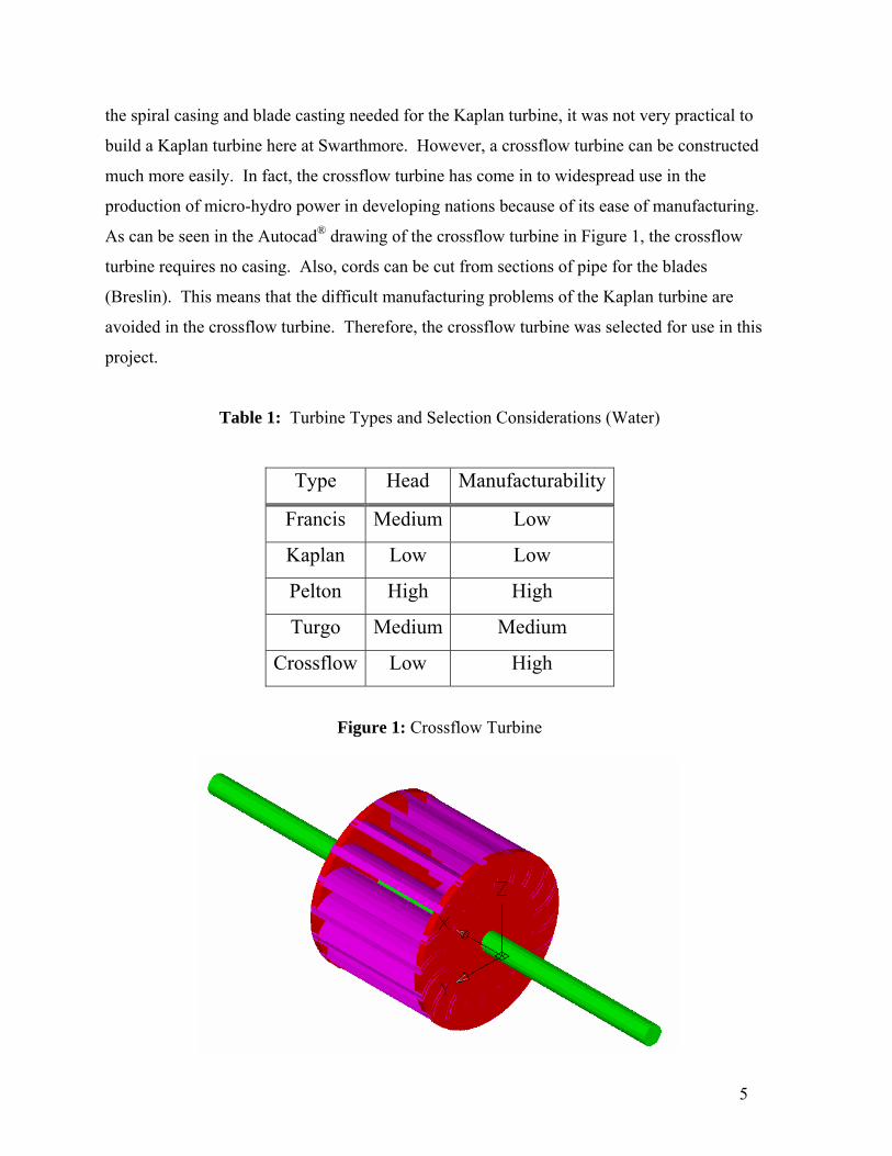
As can be seen in the Autocad® drawing of the crossflow turbine in Figure 1, the crossflow

turbine requires no casing. Also, cords can be cut from sections of pipe for the blades

(Breslin). This means that the difficult manufacturing problems of the Kaplan turbine are

avoided in the crossflow turbine. Therefore, the crossflow turbine was selected for use in this

project.

Table 1: Turbine Types and Selection Considerations (Water)

Type Head Manufacturability

Francis Medium Low

Kaplan Low Low

Pelton High High

Turgo Medium Medium

Crossflow Low High

Figure 1: Crossflow Turbine

6

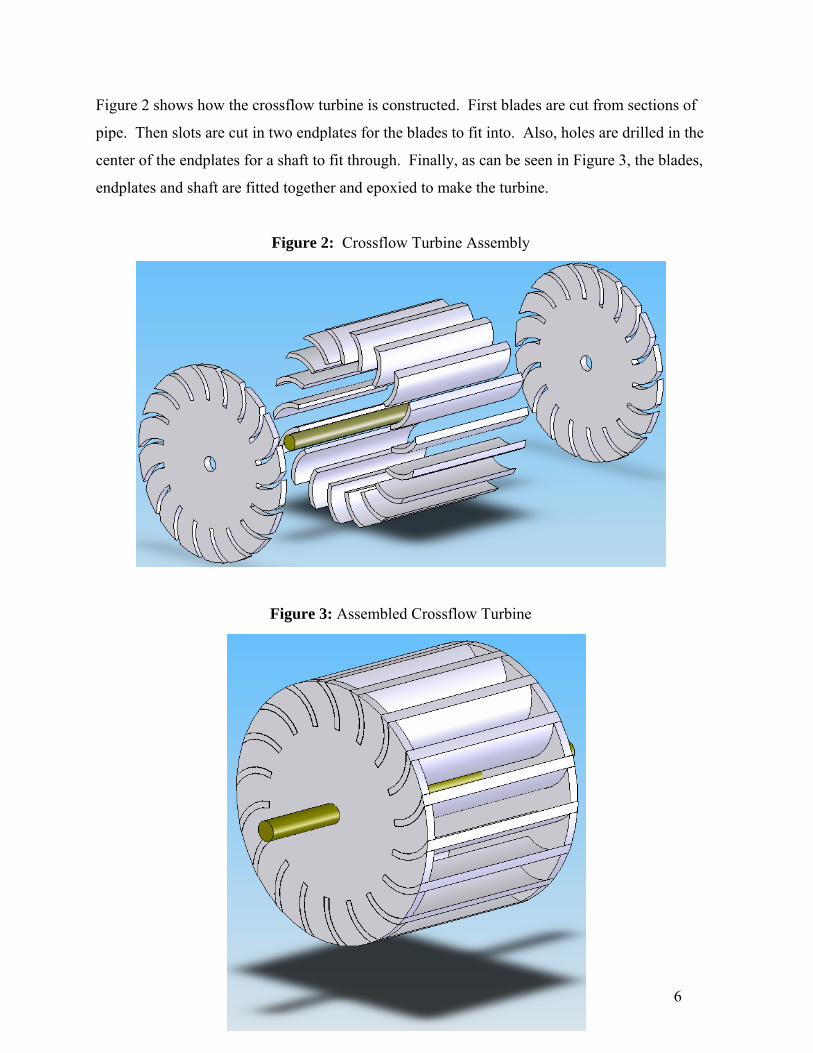
Figure 2 shows how the crossflow turbine is constructed. First blades are cut from sections of

pipe. Then slots are cut in two endplates for the blades to fit into. Also, holes are drilled in the

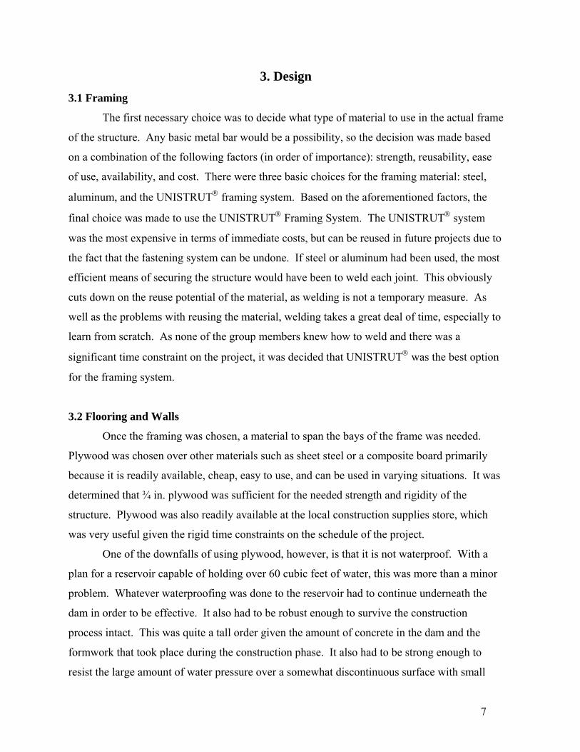
center of the endplates for a shaft to fit through. Finally, as can be seen in Figure 3, the blades,

endplates and shaft are fitted together and epoxied to make the turbine.

Figure 2: Crossflow Turbine Assembly

Figure 3: Assembled Crossflow Turbine

7

3. Design 3.1 Framing

The first necessary choice was to decide what type of material to use in the actual frame

of the structure. Any basic metal bar would be a possibility, so the decision was made based

on a combination of the following factors (in order of importance): strength, reusability, ease

of use, availability, and cost. There were three basic choices for the framing material: steel,

aluminum, and the UNISTRUT® framing system. Based on the aforementioned factors, the

final choice was made to use the UNISTRUT® Framing System. The UNISTRUT® system

was the most expensive in terms of immediate costs, but can be reused in future projects due to

the fact that the fastening system can be undone. If steel or aluminum had been used, the most

efficient means of securing the structure would have been to weld each joint. This obviously

cuts down on the reuse potential of the material, as welding is not a temporary measure. As

well as the problems with reusing the material, welding takes a great deal of time, especially to

learn from scratch. As none of the group members knew how to weld and there was a

significant time constraint on the project, it was decided that UNISTRUT® was the best option

for the framing system.

3.2 Flooring and Walls

Once the framing was chosen, a material to span the bays of the frame was needed.

Plywood was chosen over other materials such as sheet steel or a composite board primarily

because it is readily available, cheap, easy to use, and can be used in varying situations. It was

determined that ¾ in. plywood was sufficient for the needed strength and rigidity of the

structure. Plywood was also readily available at the local construction supplies store, which

was very useful given the rigid time constraints on the schedule of the project.

One of the downfalls of using plywood, however, is that it is not waterproof. With a

plan for a reservoir capable of holding over 60 cubic feet of water, this was more than a minor

problem. Whatever waterproofing was done to the reservoir had to continue underneath the

dam in order to be effective. It also had to be robust enough to survive the construction

process intact. This was quite a tall order given the amount of concrete in the dam and the

formwork that took place during the construction phase. It also had to be strong enough to

resist the large amount of water pressure over a somewhat discontinuous surface with small

8

bolts sticking up out of the plywood and sharp corners where the waterproofing material would

have no support beneath it. Given these demands and the consequences of a failure of the

waterproofing, a 1/8 in. rubber membrane was chosen to serve as a waterproof layer for the

reservoir floor and walls. It is more than adequate to withstand the water pressure over the

small discontinuities that exist on the floor and walls of the reservoir.

3.3 Bolts & Connections

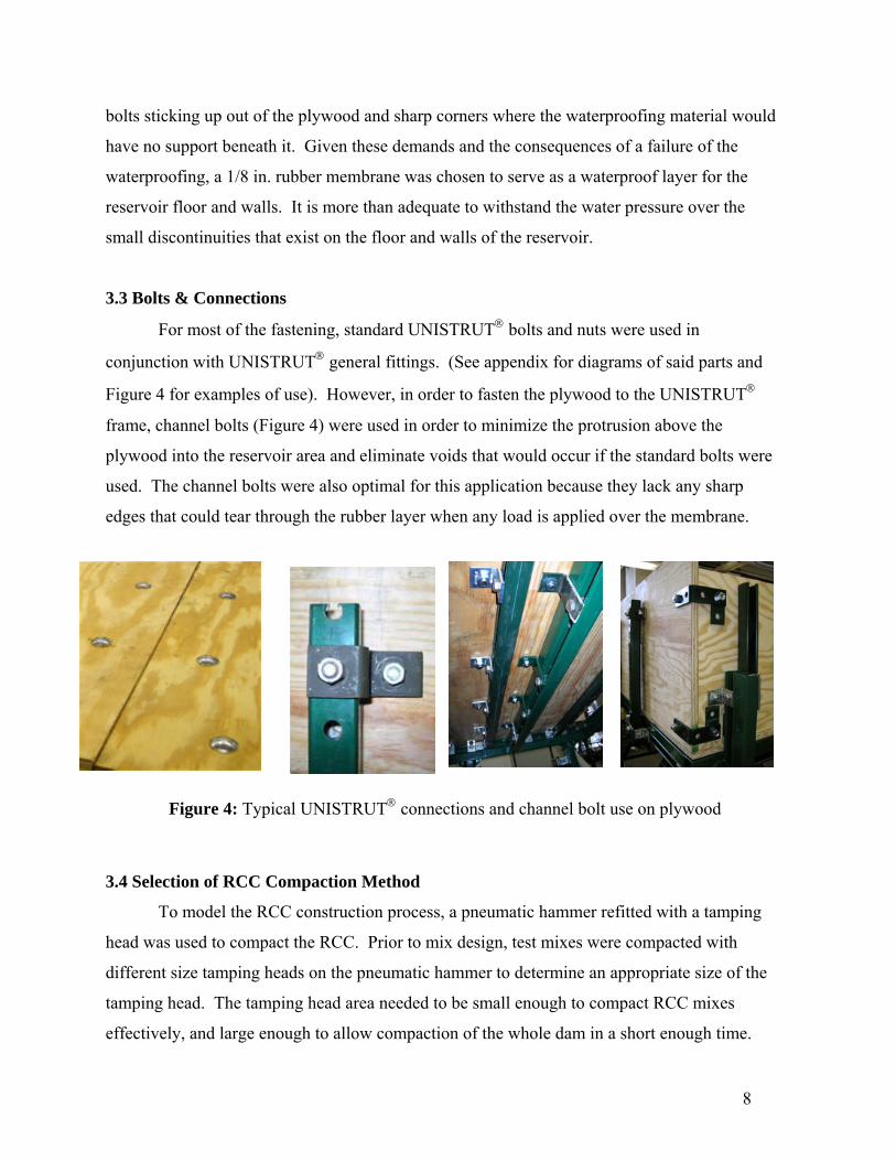
For most of the fastening, standard UNISTRUT® bolts and nuts were used in

conjunction with UNISTRUT® general fittings. (See appendix for diagrams of said parts and

Figure 4 for examples of use). However, in order to fasten the plywood to the UNISTRUT®

frame, channel bolts (Figure 4) were used in order to minimize the protrusion above the

plywood into the reservoir area and eliminate voids that would occur if the standard bolts were

used. The channel bolts were also optimal for this application because they lack any sharp

edges that could tear through the rubber layer when any load is applied over the membrane.

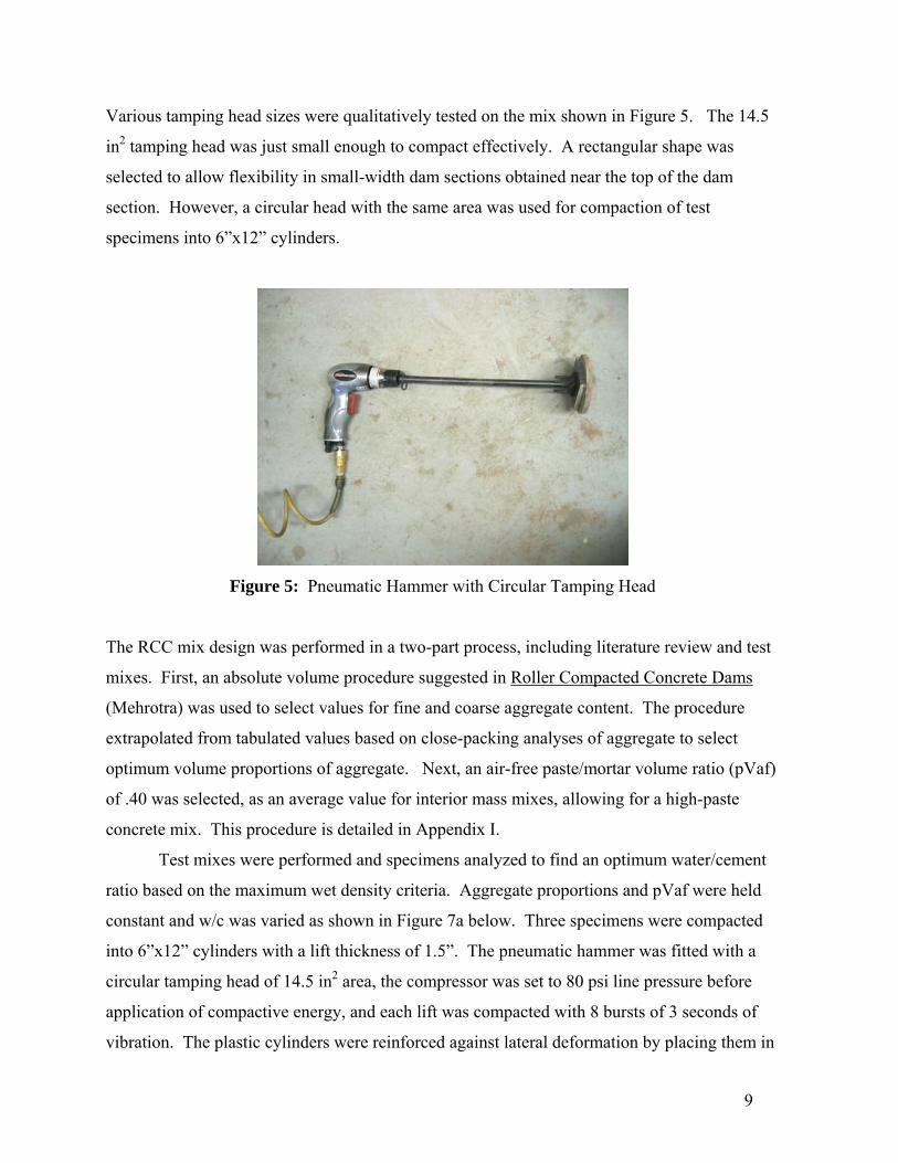
3.4 Selection of RCC Compaction Method

To model the RCC construction process, a pneumatic hammer refitted with a tamping

head was used to compact the RCC. Prior to mix design, test mixes were compacted with

different size tamping heads on the pneumatic hammer to determine an appropriate size of the

tamping head. The tamping head area needed to be small enough to compact RCC mixes

effectively, and large enough to allow compaction of the whole dam in a short enough time.

Figure 4: Typical UNISTRUT® connections and channel bolt use on plywood

9

Various tamping head sizes were qualitatively tested on the mix shown in Figure 5. The 14.5

in2 tamping head was just small enough to compact effectively. A rectangular shape was

selected to allow flexibility in small-width dam sections obtained near the top of the dam

section. However, a circular head with the same area was used for compaction of test

specimens into 6”x12” cylinders.

Figure 5: Pneumatic Hammer with Circular Tamping Head

The RCC mix design was performed in a two-part process, including literature review and test

mixes. First, an absolute volume procedure suggested in Roller Compacted Concrete Dams

(Mehrotra) was used to select values for fine and coarse aggregate content. The procedure

extrapolated from tabulated values based on close-packing analyses of aggregate to select

optimum volume proportions of aggregate. Next, an air-free paste/mortar volume ratio (pVaf)

of .40 was selected, as an average value for interior mass mixes, allowing for a high-paste

concrete mix. This procedure is detailed in Appendix I.

Test mixes were performed and specimens analyzed to find an optimum water/cement

ratio based on the maximum wet density criteria. Aggregate proportions and pVaf were held

constant and w/c was varied as shown in Figure 7a below. Three specimens were compacted

into 6”x12” cylinders with a lift thickness of 1.5”. The pneumatic hammer was fitted with a

circular tamping head of 14.5 in2 area, the compressor was set to 80 psi line pressure before

application of compactive energy, and each lift was compacted with 8 bursts of 3 seconds of

vibration. The plastic cylinders were reinforced against lateral deformation by placing them in

10

5-gallon cylinders and placing stone of >1” diameter and sand in between the cylinder wall and

the bucket wall. Each specimen was weighed and the weight of the plastic cylinder subtracted

to find its density. Upon removal from the plastic cylinders, the dimensions of the specimens

were measured, and the density calculated. The water/cement ratio producing the maximum

wet density was selected.

Figure 6: Compaction of Wet Density Specimens

Two lifts of the selected mix were then compacted into a larger mold for visual

observation. Through the plexiglass side window it was observed that significantly more voids

appeared in the concrete at 1” below the compaction surface. Thus, a fourth cylinder was cast

with a 1” lift thickness. That cylinder had an even higher wet density, therefore the 1” lift

thickness was selected.

152.5

153

153.5

154

0.4 0.5 0.6 0.7 0.8w/c (mass)

Den

sity

(lb/

ft3)

Wet density,1.5" lifts

Wet Density,1" lifts

Figure 7a: Test Mixes, Density vs. w/c

11

02000400060008000

0.4 0.45 0.5 0.55 0.6 0.65 0.7 0.75 0.8w/c (mass)

Com

pres

sive

S

treng

th (p

si)

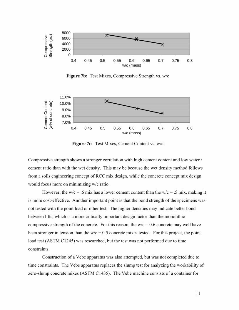
Figure 7b: Test Mixes, Compressive Strength vs. w/c

7.0%8.0%9.0%

10.0%11.0%

0.4 0.45 0.5 0.55 0.6 0.65 0.7 0.75 0.8w/c (mass)

Cem

ent C

onte

nt

(w%

of c

oncr

ete)

Figure 7c: Test Mixes, Cement Content vs. w/c

Compressive strength shows a stronger correlation with high cement content and low water /

cement ratio than with the wet density. This may be because the wet density method follows

from a soils engineering concept of RCC mix design, while the concrete concept mix design

would focus more on minimizing w/c ratio.

However, the w/c = .6 mix has a lower cement content than the w/c = .5 mix, making it

is more cost-effective. Another important point is that the bond strength of the specimens was

not tested with the point load or other test. The higher densities may indicate better bond

between lifts, which is a more critically important design factor than the monolithic

compressive strength of the concrete. For this reason, the w/c = 0.6 concrete may well have

been stronger in tension than the w/c = 0.5 concrete mixes tested. For this project, the point

load test (ASTM C1245) was researched, but the test was not performed due to time

constraints.

Construction of a Vebe apparatus was also attempted, but was not completed due to

time constraints. The Vebe apparatus replaces the slump test for analyzing the workability of

zero-slump concrete mixes (ASTM C1435). The Vebe machine consists of a container for

12

concrete mounted on a vibrating table. A vertical surcharge load is applied to the concrete, it is

vibrated, and the time until paste rises to the surface of the container is measured. This

apparatus would have allowed closer comparison with literature values for RCC mixes.

However, the effect of the pneumatic hammer was estimated in a more analytical way,

by attaching accelerometers to the tamping head as it compacted concrete. At the point of

impact with the soil, the tamping head and connection bar were modeled as a free body, only

being accelerated by the normal force of the fresh concrete. Gravity is considered negligible.

Thus, the maximum upward force and pressure on the tamping head was given by

maxmaPArea

= (Eq. 1)

where amax is the maximum upward acceleration observed by the accelerometer.

Vibratory stresses at the lift joint were estimated by modeling the dynamic load as a

static distributed load. The calculated tamping head pressure is combined with the Boussinesq

solution for a rectangular distributed loading on the surface of a linear elastic homogenous

isotropic half-space. (Poulos et al) These calculations are shown in Appendix VIII. The

results for stresses at a one-inch depth beneath the center of the tamping head are compared

with experimental values for vibratory stresses in actual RCC at a one-foot depth in Table 2.

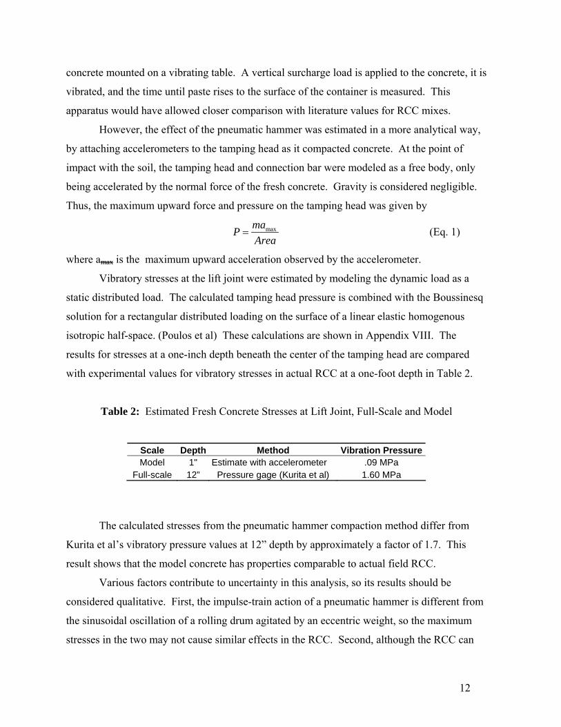
Table 2: Estimated Fresh Concrete Stresses at Lift Joint, Full-Scale and Model

Scale Depth Method Vibration Pressure Model 1" Estimate with accelerometer .09 MPa

Full-scale 12” Pressure gage (Kurita et al) 1.60 MPa

The calculated stresses from the pneumatic hammer compaction method differ from

Kurita et al’s vibratory pressure values at 12” depth by approximately a factor of 1.7. This

result shows that the model concrete has properties comparable to actual field RCC.

Various factors contribute to uncertainty in this analysis, so its results should be

considered qualitative. First, the impulse-train action of a pneumatic hammer is different from

the sinusoidal oscillation of a rolling drum agitated by an eccentric weight, so the maximum

stresses in the two may not cause similar effects in the RCC. Second, although the RCC can

13

probably be considered an infinite half-space in the lower lifts of the dam, horizontal stresses

dissipation is limited by the rigid forms in the higher, shorter lifts. Thus, stresses may be

higher in those higher lifts. Third, the lower lifts bounded on the underside by bedrock or a

cold joint will distribute stress differently and may also be affected by aggregate interlock

phenomena. However, the analysis does show qualitative correlation with the stresses in full-

scale RCC compaction.

3.5 RCC Consistency tests

The timing of lift placement was a necessary parameter for the design of the

compaction method and the downstream forms. Too long of a wait allows the formation of a

cold joint, while too short a wait causes lower unsupported layers to deform laterally under the

adjustable downstream form. To test this, a testing procedure was devised to directly assess

the ability of lower layers to resist deformation under compactive loads. The base was

removed from four 6”x12” cylinders, and two 4”x1” notches were cut into the base. Then the

cylinders were placed upside down and a layer was compacted into each. After a specified

wait time, a second layer was compacted. To remove support from the bottom layer, the

cylinder was twisted out from around the concrete layers, and replaced right-side up, thus

leaving the bottom layer unsupported. Deformation in the bottom layer was observed as the

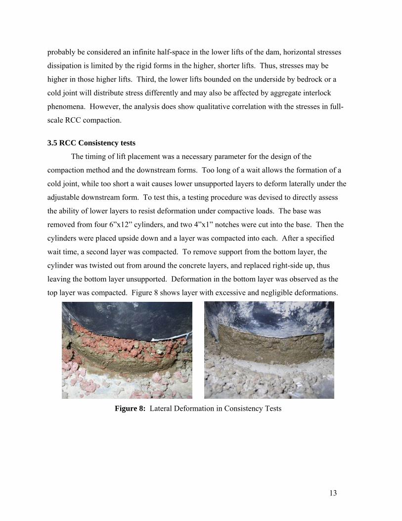
top layer was compacted. Figure 8 shows layer with excessive and negligible deformations.

Figure 8: Lateral Deformation in Consistency Tests

14

Based on these tests and an approximate setting time of 60 minutes for Type III cement

(Panarese), a three-step adjustable form design was selected, and a time window between lifts

of 45 to 60 minutes.

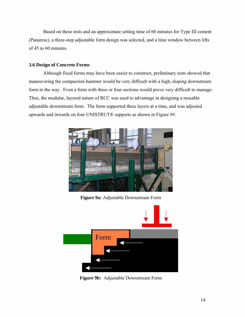
3.6 Design of Concrete Forms

Although fixed forms may have been easier to construct, preliminary tests showed that

maneuvering the compaction hammer would be very difficult with a high, sloping downstream

form in the way. Even a form with three or four sections would prove very difficult to manage.

Thus, the modular, layered nature of RCC was used to advantage in designing a reusable

adjustable downstream form. The form supported three layers at a time, and was adjusted

upwards and inwards on four UNISTRUT® supports as shown in Figure ##.

Figure 9a: Adjustable Downstream Form

Figure 9b: Adjustable Downstream Form

Form

15

3.7 Structural Load Calculations

The load calculations for the structure were fairly basic. There were only three loads to

consider in the calculations, the concrete dam, the water in the reservoir, and the self-weight of

the structure. It should be noted that dynamic construction loads were also considered, but due

to time constraints were not fully calculated in the design phase. This was deemed to be

appropriate due to the relatively smaller magnitude of these loads in comparison to the post-

construction loading.

3.8 Dam Load Calculation

The distributed load of the dam and its foundation was complicated by the fact that its

cross-section is an asymmetric trapezoid (see Figure 1-A). Across the width of the structure

the dam load was equally distributed, but across the length of the structure it is somewhat more

complicated. In the interests of time, the basic design calculations approximated this

asymmetric trapezoidal cross-section with a symmetric rectangular cross-section (see Figure 1-

B). For the purpose of the calculation of the load value, a density of 150 lb/ft^3 was used for

the concrete.

Figure 10-A: original cross-section

Figure 10-B: modified cross-section used to calculate design loading

16

3.9 Water Load Calculation

The water load was distributed equally over the rectangular area of the reservoir. The

load value was found by multiplying the volume (ft^3) of the water by its density (see equation

2). The resulting load was applied to both the plywood surface and the framing members.

* wMax load V ρ= (Eq.2)

3.10 Dynamic Load Calculation

Upon discussion, it was decided that the expected dynamic loads were not large enough

to be significant factors in any of the design calculations except for stabilization purposes.

Therefore a detailed dynamic calculation was not carried out due to time constraints.

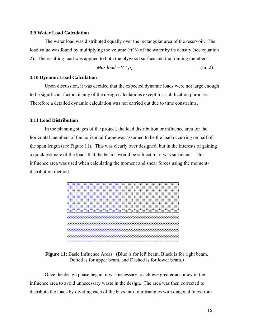
3.11 Load Distribution

In the planning stages of the project, the load distribution or influence area for the

horizontal members of the horizontal frame was assumed to be the load occurring on half of

the span length (see Figure 11). This was clearly over designed, but in the interests of gaining

a quick estimate of the loads that the beams would be subject to, it was sufficient. This

influence area was used when calculating the moment and shear forces using the moment-

distribution method.

Once the design phase began, it was necessary to achieve greater accuracy in the

influence area to avoid unnecessary waste in the design. The area was then corrected to

distribute the loads by dividing each of the bays into four triangles with diagonal lines from

Figure 11: Basic Influence Areas. (Blue is for left beam, Black is for right beam, Dotted is for upper beam, and Dashed is for lower beam.)

17

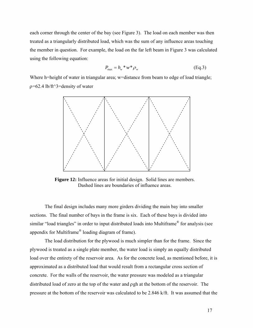
each corner through the center of the bay (see Figure 3). The load on each member was then

treated as a triangularly distributed load, which was the sum of any influence areas touching

the member in question. For example, the load on the far left beam in Figure 3 was calculated

using the following equation:

max * *w wP h w ρ= (Eq.3)

Where h=height of water in triangular area; w=distance from beam to edge of load triangle;

ρ=62.4 lb/ft^3=density of water

The final design includes many more girders dividing the main bay into smaller

sections. The final number of bays in the frame is six. Each of these bays is divided into

similar “load triangles” in order to input distributed loads into Multiframe® for analysis (see

appendix for Multiframe® loading diagram of frame).

The load distribution for the plywood is much simpler than for the frame. Since the

plywood is treated as a single plate member, the water load is simply an equally distributed

load over the entirety of the reservoir area. As for the concrete load, as mentioned before, it is

approximated as a distributed load that would result from a rectangular cross section of

concrete. For the walls of the reservoir, the water pressure was modeled as a triangular

distributed load of zero at the top of the water and ρgh at the bottom of the reservoir. The

pressure at the bottom of the reservoir was calculated to be 2.846 k/ft. It was assumed that the

Figure 12: Influence areas for initial design. Solid lines are members. Dashed lines are boundaries of influence areas.

18

outward pressure of the concrete would never exceed the pressure from the water, so the water

pressure was the overriding factor.

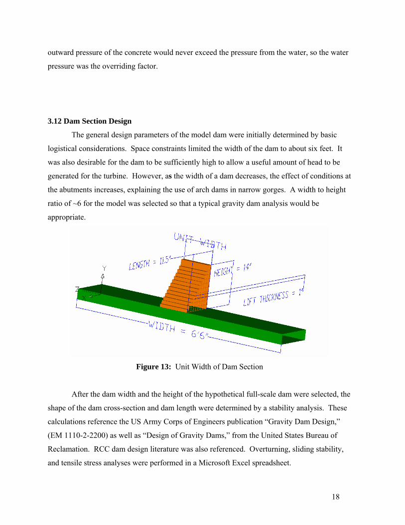
3.12 Dam Section Design

The general design parameters of the model dam were initially determined by basic

logistical considerations. Space constraints limited the width of the dam to about six feet. It

was also desirable for the dam to be sufficiently high to allow a useful amount of head to be

generated for the turbine. However, as the width of a dam decreases, the effect of conditions at

the abutments increases, explaining the use of arch dams in narrow gorges. A width to height

ratio of ~6 for the model was selected so that a typical gravity dam analysis would be

appropriate.

Figure 13: Unit Width of Dam Section

After the dam width and the height of the hypothetical full-scale dam were selected, the

shape of the dam cross-section and dam length were determined by a stability analysis. These

calculations reference the US Army Corps of Engineers publication “Gravity Dam Design,”

(EM 1110-2-2200) as well as “Design of Gravity Dams,” from the United States Bureau of

Reclamation. RCC dam design literature was also referenced. Overturning, sliding stability,

and tensile stress analyses were performed in a Microsoft Excel spreadsheet.

19

Because the concrete mix design was performed concurrently with the dam section

design, the material properties for the final RCC mix were unavailable during the design

process. Thus, the stresses in the dam were evaluated conservatively at first, and compared

with experimental values for the lift interface bond strength and other properties of the

concrete mix subsequent to constructing the model.

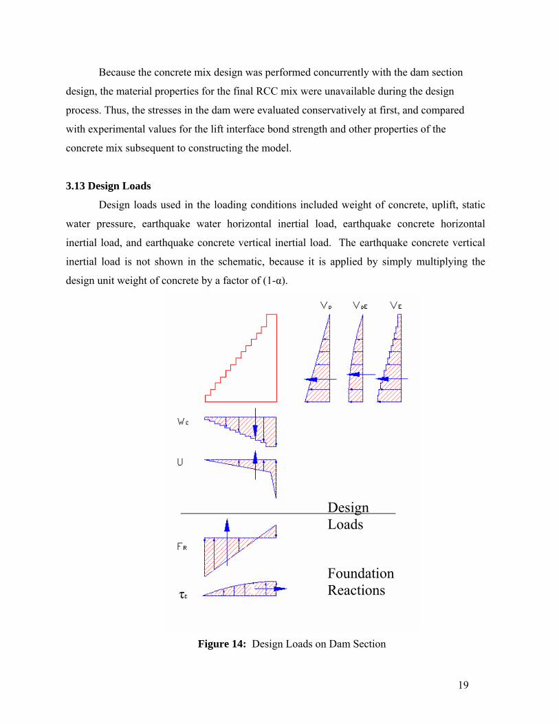
3.13 Design Loads

Design loads used in the loading conditions included weight of concrete, uplift, static

water pressure, earthquake water horizontal inertial load, earthquake concrete horizontal

inertial load, and earthquake concrete vertical inertial load. The earthquake concrete vertical

inertial load is not shown in the schematic, because it is applied by simply multiplying the

design unit weight of concrete by a factor of (1-α).

Figure 14: Design Loads on Dam Section

Design Loads

Foundation Reactions

20

3.14 Loading Conditions

Two sets of loading conditions were considered for the analysis of both the model-scale

dam as well as the hypothetical full-scale dam, for a total of four analyses. These are the usual

or normal operation condition, and the extreme loading condition. Figure ## shows a

schematic diagram of all forces acting on the dam for normal operation (usual loading) on the

full-scale dam. A description of the loading conditions is shown below.

Full-Scale Load Condition No. 1 - Usual loading condition

(a) Pool elevation at spillway crest

(b) Uplift (drains operational)

Full-Scale Load Condition No. 2 - Extreme loading condition

(a) Pool elevation at spillway crest

(b) Uplift (drains operational)

(c) Maximum Credible Earthquake inertial loading

Model-Scale Load Condition No. 1 - Usual loading condition

(a) Pool elevation at flow height above spillway crest

(b) Zero uplift

(c) Impact disturbance loading

Model-Scale Load Condition No. 2 - Extreme loading condition

(a) Pool elevation at flow height above spillway crest

(b) Full uplift

(c) Impact disturbance loading

Earthquake values were determined for a Design Basis Earthquake and a Maximum

Credible Earthquake, based on the eastern PA region. Since some portions of eastern PA are

coded “2A” by the Army Corps of Engineers’ Uniform Building Code Seismic Zone Map, and

this value corresponds to an α = 0.15, this value was selected as the DBE acceleration. The

MCE acceleration was taken from the USGS Seismic Hazard Map of PA, with an α = 0.20.

For the model analysis, inertial loads were assumed to account for people or objects impacting

the support structure.

In the absence of drains in the foundation, hydraulic uplift pressure is considered to act

over the entire base, decreasing linearly from full hydrostatic pressure at the upstream face to

21

zero pressure at the downstream face. However, this loading makes design uneconomical, and

in practice, foundation drains are used to mitigate the effects of uplift. Drains are horizontal

transverse pipes cast near the base of the dam at regular intervals to draw and release

pressurized water from inside the upstream face before full hydrostatic pressure can build up

within the concrete.

With drains effective, uplift decreases from full hydrostatic pressure at the upstream

face to a fraction of the full uplift value at the line of drains. Thus, from the line of drains to

the downstream face, uplift pressure is equal to (1 – efficiencydrains)*(full uplift value). Uplift

(U) is shown in Figure 14 above. The highest allowable design drains efficiency is 66%.

Thus, to select a more conservative design for the model dam, a drains efficiency of 40% was

assumed for the usual and unusual loadings in the full-scale analysis. For the model analysis,

the expected usual loading condition was zero uplift, and an extreme condition of full uplift

was considered as well.

3.15 Gravity Dam Method of Analysis

For design based on overturning, sliding, and allowable stress, the dam was modeled

according to the gravity method for stress and stability analysis. This method is commonly

used for preliminary design of dams, as well as for some final designs of straight gravity dams.

See Appendix II for calculation examples and tabulated values.

The gravity dam method requires the following five assumptions:

1. The concrete in the dam is a homogenous, isotropic, and uniformly elastic material.

This assumption should be accurate for normal elastic behavior of RCC in

compression. However, the bond between layers of RCC at lift joints is a critical

factor. Thus, the lift joints are critical failure surfaces for analysis of tensile and sliding

failure states. But, the properties of the concrete at all locations but the lift interface is

considered homogenous. Thus, this first assumption is considered valid for analysis of

stress distributions, although the bond strength is considered in selecting the failure

surface and the allowable stress.

2. There are no differential movements of foundation or abutments due to water loads on the

reservoir walls and floors.

22

This second group of assumptions is certainly sound for the model-scale dam, and is

considered valid for the hypothetical full-scale dam.

3. All loads are carried by the gravity action of vertical, parallel side cantilevers which

receive no support from the adjacent elements on either side. (These cantilevers are shown

as transverse sections of the dam, with a thickness of unit width.)

This is commonly the principal sticking point for requiring a three-dimensional finite

element analysis, a “Trial-Load Twist Analysis,” or some other 3D method. Long

dams may have no way to release the buildup of bending moments and flexural stresses

between adjacent cantilever sections. Longitudinally transmitted shear forces and

flexural stresses between the cantilevers result from temperature strains acting against

internal and foundation restraints. For the model-scale dam, the rubber abutments

would release any such stresses. With respect to the full-scale dam, this paper can be

considered a preliminary analysis neglecting longitudinally transmitted stresses.

4. Unit vertical pressures, or normal stresses on horizontal planes, vary uniformly as a

straight line from the upstream face to the downstream face.

5. Horizontal shear stresses have a parabolic variation across horizontal planes from the

upstream face to the downstream face of the dam.

According to the USBR report, the final two assumptions are valid except for

horizontal planes near the base where stresses reflect foundation yielding. And, in

those cases as well, the effects can usually be neglected for small and medium height

dams.

3.16 Stability Considerations

There are three basic stability requirements for a gravity dam, in all loading states:

1. Safety against overturning at any horizontal plane through or beneath the structure

2. Safety against sliding on horizontal or near-horizontal plane through or beneath the

structure

3. Allowable unit stresses in the concrete or foundation are not exceeded

Those requirements are accounted for by the following methods:

23

Safety against Overturning

The location of the resultant of forces acting above a horizontal section of the dam,

excepting the non-uplift vertical reaction, is determined. The distance x of the resultant from

the downstream toe of this section is found by Equation 4,

Mx

V= ∑∑

(Eq. 4)

where M refers to moments of all forces about the toe, and V refers to the sum of all

horizontal forces. For safety against overturning, the Army Corps design guide requires that

this resultant lie within the central third of the dam section for usual loading conditions, and

within the dam section for extreme loading conditions.

The resultant being within the central third means that the entire horizontal section is in

compression, with no flexural tension occurring in the cantilever. This result follows from

assumption (4) of the gravity method. With exactly zero compression in the upstream end of

the section, the FR distribution flattens from a trapezoid into a triangle, whose centroid is a

distance of L/3 from the downstream end. If the resultant moves past the toe, the means that

the FR resultant is tension, and the section is unstable.

Safety against Sliding

(Eq. 5)

Sliding safety factor Q is calculated as the ratio of resisting to driving forces, according to

equation (2). C is the unit cohesion at the failure surface and A is the area of failure surface. φ

is the angle of internal friction at the failure surface. N refers to the downward normal forces

transmitted to the foundation. U is uplift, which is in opposition to N and thus decreases the

magnitude of the friction term in the calculation. Finally, V is the sum of horizontal loads on

the dam section.

Allowable stress

Concrete is strong in compression, so exceeding compressive stress is not a concern in

designing a medium-small concrete gravity dam. However, concrete is weak in tension, and a

( ) tanCA N UQ

Vϕ+ +

= ∑ ∑∑

24

gravity dam depends on its weight to resist moments and forces placed upon it; there is no

structural tension reinforcement in gravity dams. RCC dams are especially vulnerable at joints

between lifts. Even if the monolithic concrete has a high strength, if there are significant latent

voids between lifts, the effective area in tension becomes very small. Thus, the Army Corps

engineering manual on Roller Compacted Concrete (Army Corps, RCC, Table 4-3) provides

empirical equations published by Robert Cannon in 1996 to estimate the tensile strength at lift

joints of RCC with different characteristics.

Since a Vebe table was unavailable to assess the consistence of the RCC, the most

conservative relation of ft to f‘c available in the table was used. For a Vebe time of > 30 sec,

less workable consistency, without a bedding mortar layer, a design lift joint tensile strength of

ft = .015*f’c was used.

3.17 Dam Design Calculations

Design calculations for the model-extreme and full-scale-extreme loading conditions

are shown in Appendix II, along with a full tabulation of values for all loading conditions.

3.18 Miscellaneous Appurtenances and Procedures

Since it is very difficult to embed appurtenances into RCC, especially flexible ones like

PVC piping, the horizontal penstock was cast in a block of conventional concrete directly on

bedrock before casting of RCC.

RCC dams are vulnerable to seepage along the lift joints. For this reason, most RCC

dams include a 1.5’ to 3’ thick layer of conventional or precast facing concrete, and sometimes

even a plastic liner. Since this would have been difficult on the model scale, sealing of the

upstream face was accomplished with a spray-on primer and a 1/8” coating of asphalt and

solvent-based elastic sealant. This tar was also used to seal the rubber seams in the reservoir

and the wooden plunge pool for the spillway.

Problems with the air compressor during construction required the treating of a cold

joint when construction resumed. First, the surface was wire brushed and air-blown clean.

Then, a 1:1 volume ratio sand/cement grout was prepared and a ¼” layer was troweled onto the

previous layer’s cured surface. This provided a maximum bond between the cured and fresh

concrete layers.

25

After construction, a 20” width of the downstream face was covered with grout to make

a stepped spillway. To make a well-leveled spillway precisely at the designed 14” above

bedrock, a handheld wheel grinder was used to precisely level that portion of the crest.

Adjacent portions of the crest were then raised with a small amount of grout to allow the water

to rise to the design 14.5” above bedrock.

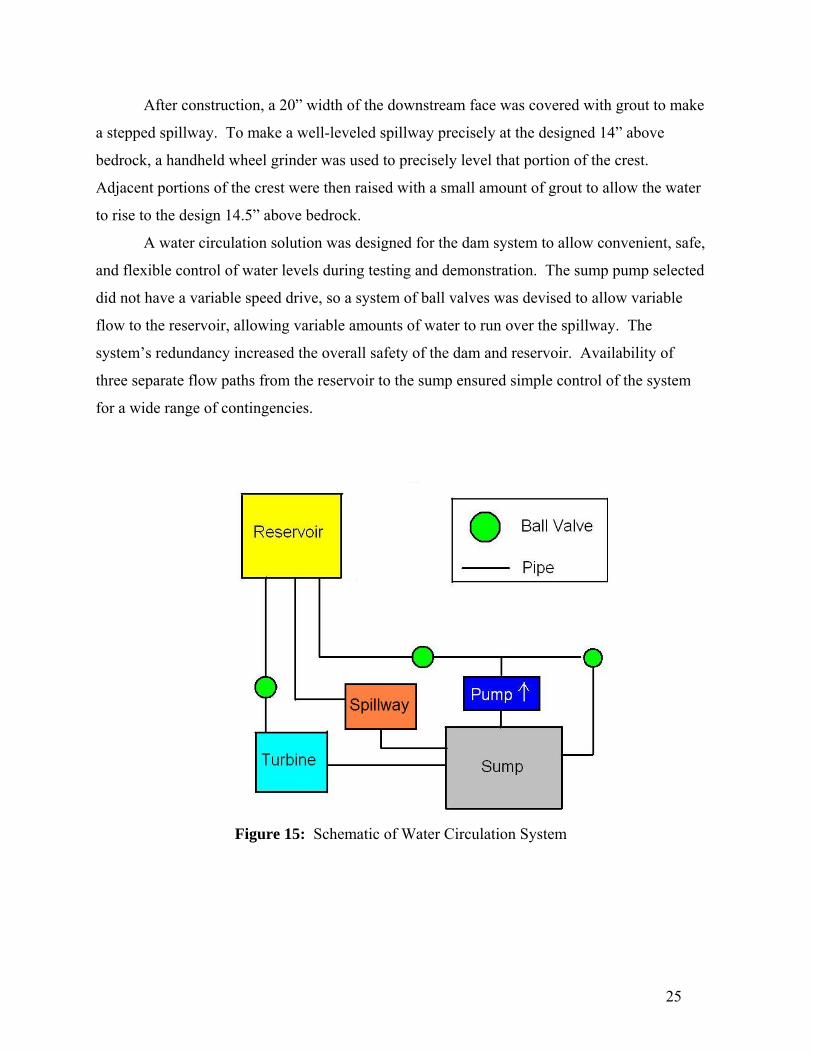
A water circulation solution was designed for the dam system to allow convenient, safe,

and flexible control of water levels during testing and demonstration. The sump pump selected

did not have a variable speed drive, so a system of ball valves was devised to allow variable

flow to the reservoir, allowing variable amounts of water to run over the spillway. The

system’s redundancy increased the overall safety of the dam and reservoir. Availability of

three separate flow paths from the reservoir to the sump ensured simple control of the system

for a wide range of contingencies.

Figure 15: Schematic of Water Circulation System

26

3.17 Water Flow Calculations

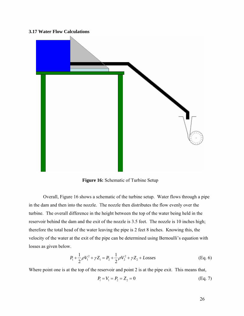
Figure 16: Schematic of Turbine Setup

Overall, Figure 16 shows a schematic of the turbine setup. Water flows through a pipe

in the dam and then into the nozzle. The nozzle then distributes the flow evenly over the

turbine. The overall difference in the height between the top of the water being held in the

reservoir behind the dam and the exit of the nozzle is 3.5 feet. The nozzle is 10 inches high;

therefore the total head of the water leaving the pipe is 2 feet 8 inches. Knowing this, the

velocity of the water at the exit of the pipe can be determined using Bernoulli’s equation with

losses as given below.

2 21 1 1 2 2 2

1 12 2

P V Z P V Z Lossesρ γ ρ γ+ + = + + + (Eq. 6)

Where point one is at the top of the reservoir and point 2 is at the pipe exit. This means that,

1 1 2 2 0P V P Z= = = = (Eq. 7)

27

Therefore, 2 2

2 21 2 2L

V VlZ f Kg D g

⎛ ⎞= + +⎜ ⎟⎝ ⎠

(Eq. 8)

Where f is the friction factor and LK is the sum of the coefficients of minor losses. The length

of the pipe was estimated to be 4 feet 4 inches given the length of the dam as well as the fact

that the pipe slopes down at a 45 degree angle. The minor loss coefficients were taken to be

0.5 for the entrance and 0.4 for each of the 45 degree angles (Munson 453). Therefore,

1.3LK = . Also, the pipe has a diameter of 2 inches and a roughness of zero because it is

plastic. Therefore,

( ) ( )2

24.332.67 2.31/ 6 2 32.2

Vf⎛ ⎞

= +⎜ ⎟⎜ ⎟⎝ ⎠

(Eq. 9)

Assuming a friction factor of zero, 2

2

2

5

74.67V = 8.64 ft/s

Re 1.2 10

V

VDρμ

=

= = ×

(Eq. 10)

Given a Reynolds number of 51.2 10× and smooth pipe, the friction factor from the moody

diagram is 0.0172 (Munson 436). Substituting this back into Bernoulli’s equation, the velocity

is reduced to 7.9 ft/s. This velocity returns a Reynolds number of 51.1 10× and a friction factor

of 0.0176. Using this friction factor in the Bernoulli relation, the velocity is again 7.9 ft/s.

Therefore, 7.9 ft/s is the theoretical velocity of the water as it exits the pipe. This velocity can

then be used to determine the volume flow of the water as it leaves the pipe because,

2

4Q D Vπ= (Eq. 11)

Therefore, with a velocity of 7.9 ft/s and a pipe diameter of 2 inches, the volume flow of the

water at the exit of the pipe should be 0.172 ft3/s. By knowing the volume flow and the head

of the water entering the turbine, the turbine can then be optimized to run most efficiently as

shown below.

28

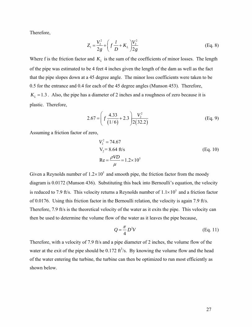
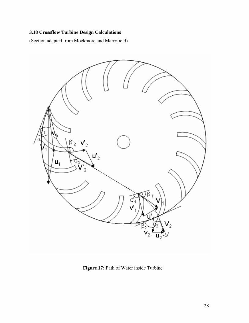
3.18 Crossflow Turbine Design Calculations

(Section adapted from Mockmore and Marryfield)

Figure 17: Path of Water inside Turbine

29

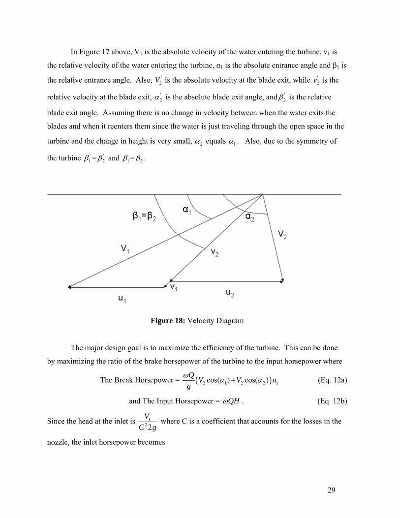
In Figure 17 above, V1 is the absolute velocity of the water entering the turbine, v1 is

the relative velocity of the water entering the turbine, α1 is the absolute entrance angle and β1 is

the relative entrance angle. Also, '2V is the absolute velocity at the blade exit, while '

2v is the

relative velocity at the blade exit, '2α is the absolute blade exit angle, and '

2β is the relative

blade exit angle. Assuming there is no change in velocity between when the water exits the

blades and when it reenters them since the water is just traveling through the open space in the

turbine and the change in height is very small, '2α equals '

1α . Also, due to the symmetry of

the turbine '1β = '

2β and 1β = 2β .

Figure 18: Velocity Diagram

The major design goal is to maximize the efficiency of the turbine. This can be done

by maximizing the ratio of the brake horsepower of the turbine to the input horsepower where

The Break Horsepower = ( )2 1 2 2 1cos( ) cos( )Q V V ugω α α+ (Eq. 12a)

and The Input Horsepower = QHω . (Eq. 12b)

Since the head at the inlet is 12 2V

C g where C is a coefficient that accounts for the losses in the

nozzle, the inlet horsepower becomes

30

12 2QV

C gω . (Eq. 12c)

From the velocity diagram (Figure 18) it can be seen that

2 2 2 2 2cos( ) cos( )V v uα β= − (Eq. 13) and 1 1 1 1 1cos( ) cos( )v V uβ α= − . (Eq. 14)

Also,

2 1v vψ= (Eq. 15)

where ψ a coefficient accounting for the friction loss in the turbine (typically equal to about

0.98). Therefore, substituting (13), (14), and (15) into the break horsepower equation and

rearranging terms, the horsepower output becomes

( )1 21 1 1

1

cos( )cos( ) 1cos( )

Qu V ug

ω βα ψβ

⎛ ⎞⎛ ⎞⎛ ⎞− +⎜ ⎟⎜ ⎟⎜ ⎟⎜ ⎟⎝ ⎠ ⎝ ⎠⎝ ⎠

. (Eq. 16)

Therefore, the efficiency of the turbine which is the ratio of the break horsepower to the input

horsepower is 2

1 2 11

1 1 1

2 cos( )1 cos( )cos( )

C u ueV V

βψ αβ

⎛ ⎞⎛ ⎞⎛ ⎞= + −⎜ ⎟⎜ ⎟⎜ ⎟⎝ ⎠⎝ ⎠⎝ ⎠

. (Eq. 17a)

However, because 1β = 2β , the efficiency simplifies to

( )2

1 11

1 1

2 1 cos( )C u ueV V

ψ α⎛ ⎞ ⎛ ⎞

= + −⎜ ⎟ ⎜ ⎟⎝ ⎠ ⎝ ⎠

. (Eq. 17b)

Treating 1

1

uV

as a variable and differentiating both sides of equation (16b) by 1

1

uV

we find that

( )2 11

11

1

2 1 cos( ) 2 ue CVu

V

ψ α⎛ ⎞∂

= + −⎜ ⎟⎛ ⎞ ⎝ ⎠∂ ⎜ ⎟⎝ ⎠

. (Eq. 18)

Therefore, setting 1

1

euV

∂⎛ ⎞

∂ ⎜ ⎟⎝ ⎠

equal to zero to find the maximum and solving for 1

1

uV

we find that

1

1

uV

= 1cos( )2α . (Eq. 19)

Substituting this back into equation (17b) we find that

31

( )2 21

1 1 cos ( )2Maxe C ψ α= + . (Eq. 20)

Therefore, the efficiency is maximized when α1 = 0. However, is not possible to achieve an

entrance angle of zero degrees. In fact, Donat Banki, one of the pioneers in the development of

the crossflow turbine, found that the smallest angle that is easy to achieve is about 16º.

Therefore, α1 was set to 16º in our design. Substituting this back into equation (20) and using

0.98 and an estimate for C and ψ, the maximum efficiency of the turbine becomes 87.8%.

Rearranging equation (19) we find that

1 1 11 cos( )2

u V α= . (Eq. 21)

Therefore, using equation (21) and the velocity diagram (Figure 18),

1 1tan( ) 2 tan( )β α= . (Eq. 22)

Substituting 1 16α = ° into equation (22) and solving for 1β , we find that 1β is approximately

equal to 30°. Also, if we assume a negligible shock loss at the entrance, then '2β must equal

90° because the inner tip of the blade must be radial. Therefore, all of the design angles of the

blades are known for the Crossflow turbine.

Next, equations for the size of the turbine must be determined. In general, the

tangential velocity of a rotating circular object is equal to the rotational speed of the object

times the perimeter of the rotating object. Therefore,

11 (12)(60)

D Nu π= (Eq. 23)

where 1u is the tangential velocity in feet per second, 1D is the diameter in inches and N is the

rotational speed in rotations per minute. Combining equation 23 with equation 21, we find that

11 1

1 cos( )2 (12)(60)

D NV πα = . (Eq. 24)

Also, from Bernoulli’s equation we know that 2 21 2V C gH= (Eq. 25a). Therefore,

1 21 (2 )V C gH= (Eq. 25b). Substituting equation (25b) back into equation (24), we find that

32

1 2 11

1 (2 ) cos( )2 (12)(60)

D NC gH πα = . (Eq. 26)

Substituting C = 0.98 and 1α = 16° in to equation (26) and solving for 1D the equation

becomes 1 2

1862HD

N= . (Eq. 27)

The length of the crossflow turbine can also be determined by knowing the volume flow and

the head of the water as well as the diameter of the turbine. First, the volume flow is equal to

the velocity of the water through the nozzle times the nozzle area. Therefore,

( )1 22144

oCs LQ gH⎛ ⎞= ⎜ ⎟⎝ ⎠

(Eq. 28)

where os is the nozzle thickness in inches and L is the nozzle width in inches. However, the

thickness of the nozzle can generally be expressed as a fraction of the turbine diameter,

1os kD= (Eq. 29) where k as been experimentally determined to be about 0.087 (mean value

determined by Dr. Banki). Therefore, substituting equation (27) into equation (28) and solving

for L we find that

1 21

210.6QLD H

= . (Eq. 30)

The curvature of the blade can found from Figure 5 where the blade is a cord of a circle

whose center lies at the intersection of a line perpendicular to the relative velocity at the blade

entrance (line AC) and a line perpendicular to the relative velocity at the blade exit (line BC).

From Figure 5, it can be seen that

( ) ( ) ( ) ( ) ( )2 2 2 2

12 cosOB BC AO AC AOAC β+ = + − . (Eq. 31)

However, 1 2AO = r , BO = r , and AC = BC = ρ . Therefore,

( ) ( )( )

2 21 2

1 12 cos

r r

rρ

β

⎡ ⎤−⎣ ⎦= (Eq. 32)

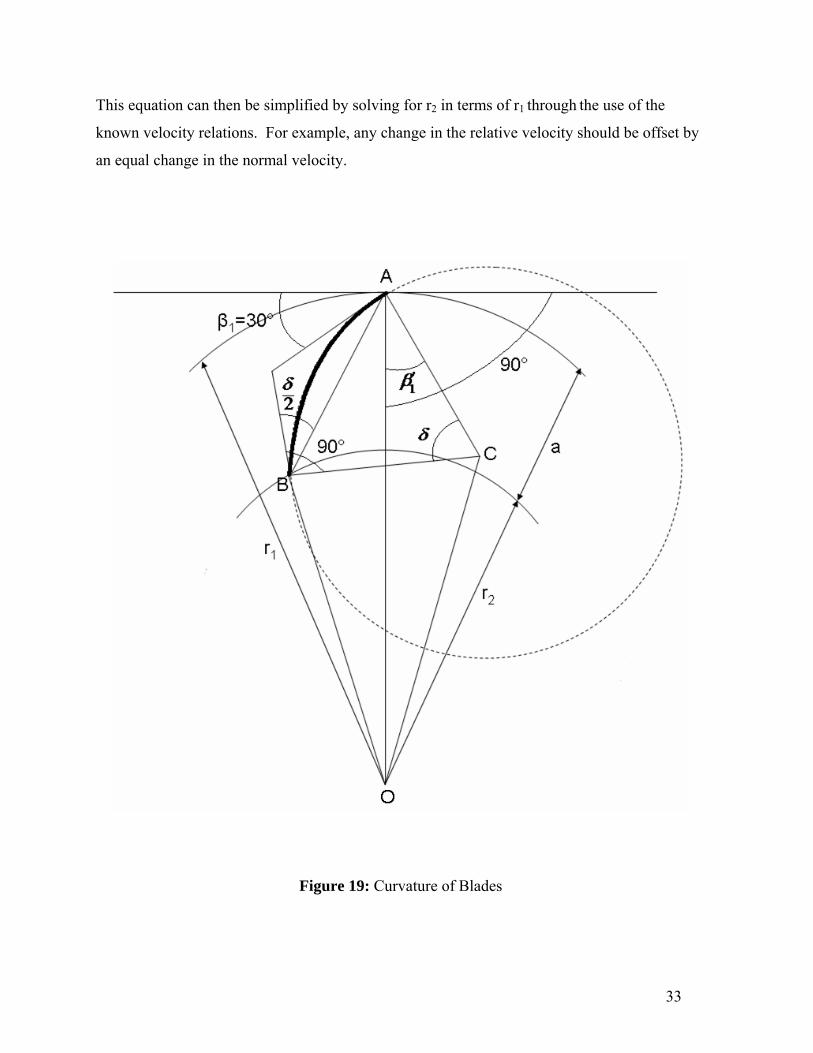
33

This equation can then be simplified by solving for r2 in terms of r1 through the use of the

known velocity relations. For example, any change in the relative velocity should be offset by

an equal change in the normal velocity.

Figure 19: Curvature of Blades

34

Therefore,

( ) ( ) ( ) ( )2 22 2' '1 2 1 2v v u u− = − (Eq. 33a)

or ( ) ( ) ( ) ( )2 22 2 ' '1 1 2 20 v u v u= − − + . (Eq. 33b)

Also, because mass must be conserved, the volume flow at the entrance and exit of the blade

must be equal therefore

' 12 1

2

sv vs

⎛ ⎞= ⎜ ⎟

⎝ ⎠ (Eq. 34)

Where s1 is the jet width at the blade entrance and s2 is the jet width at the blade exit.

However, the jet thickness can also be expressed in terms of the blade spacing. Therefore, if

the jet thickness is measured at a right angle to the relative velocity,

1 1 1sin( )s t β= (35a) and 2 2 2sin( )s t β= (Eq. 35b)

Where t1 is the blade spacing at the blade entrance and t2 is the blade spacing at the blade exit.

However, 22 1

1

rt tr

⎛ ⎞= ⎜ ⎟⎝ ⎠

and 2 90β = so equation (35b) becomes

22

1

rs tr

⎛ ⎞= ⎜ ⎟

⎝ ⎠ . (Eq. 36)

Therefore, Substituting equations (35a) and (36) into equation (34), equation (34) becomes

' 12 1 1

2

sin( )rv vr

β⎛ ⎞

= ⎜ ⎟⎝ ⎠

. (Eq. 37)

Also, the normal velocities are scaled by their distance from the center of rotation due to

differences in centrifugal forces. Therefore,

' 22 1

1

ru ur

⎛ ⎞= ⎜ ⎟

⎝ ⎠. (Eq. 38)

Substituting these values of '2v and '

2u into equation (33b), the equation becomes

2 22 2 2 2 21 21 1 1 1 1

2 1

0 sin ( )r rv u v ur r

β⎛ ⎞ ⎛ ⎞

= − + + −⎜ ⎟ ⎜ ⎟⎝ ⎠ ⎝ ⎠

. (Eq. 39)

Multiplying through by 2

1

rr

⎛ ⎞⎜ ⎟⎝ ⎠

and dividing through by 21u the equation becomes

35

4 2 2 222 1 2 1

11 1 1 1

0 1 sin ( )r v r vr u r u

β⎡ ⎤⎛ ⎞ ⎛ ⎞ ⎛ ⎞ ⎛ ⎞⎢ ⎥= − − −⎜ ⎟ ⎜ ⎟ ⎜ ⎟ ⎜ ⎟⎢ ⎥⎝ ⎠ ⎝ ⎠ ⎝ ⎠ ⎝ ⎠⎣ ⎦

. (Eq. 40)

From equation (21), 1 1 11 cos( )2

u V α= and from equation (3) 1 1 1 1 1cos( ) cos( )v V uβ α= − ,

therefore, 1 1cos( )v β = 1 1 1 1 1 1 11 1cos( ) cos( ) cos( )2 2

V V V uα α α− = = . This means that,

1

1 1

1cos( )

vu β

= . (Eq. 41)

Substituting this into equation (40), the equation becomes 4 2 2 2

22 21

1 1 1 1

1 10 1 sin ( )cos( ) cos( )

r rr r

ββ β

⎡ ⎤⎛ ⎞ ⎛ ⎞ ⎛ ⎞ ⎛ ⎞⎢ ⎥= − − −⎜ ⎟ ⎜ ⎟ ⎜ ⎟ ⎜ ⎟⎢ ⎥⎝ ⎠ ⎝ ⎠ ⎝ ⎠ ⎝ ⎠⎣ ⎦

. (Eq. 42)

Since, 1 30β = and 1 16α = , equation (41) simplifies to

4 2

2 2

1 1

0 0.33 0.332r rr r

⎛ ⎞ ⎛ ⎞= + −⎜ ⎟ ⎜ ⎟⎝ ⎠ ⎝ ⎠

. (Eq. 43)

Therefore, 2

2

1

0.453rr

⎛ ⎞=⎜ ⎟

⎝ ⎠ (Eq. 44)

and

2 10.66r r= . (Eq. 45)

Substituting equation (45) back into equation (32), equation (32) simplifies to

10.326rρ = . (Eq. 46)

36

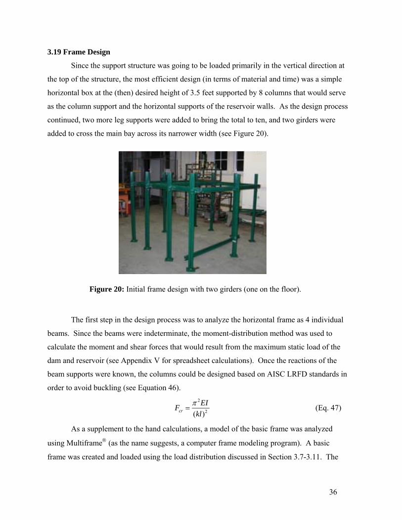
3.19 Frame Design

Since the support structure was going to be loaded primarily in the vertical direction at

the top of the structure, the most efficient design (in terms of material and time) was a simple

horizontal box at the (then) desired height of 3.5 feet supported by 8 columns that would serve

as the column support and the horizontal supports of the reservoir walls. As the design process

continued, two more leg supports were added to bring the total to ten, and two girders were

added to cross the main bay across its narrower width (see Figure 20).

The first step in the design process was to analyze the horizontal frame as 4 individual

beams. Since the beams were indeterminate, the moment-distribution method was used to

calculate the moment and shear forces that would result from the maximum static load of the

dam and reservoir (see Appendix V for spreadsheet calculations). Once the reactions of the

beam supports were known, the columns could be designed based on AISC LRFD standards in

order to avoid buckling (see Equation 46). 2

2( )crEIF

klπ

= (Eq. 47)

As a supplement to the hand calculations, a model of the basic frame was analyzed

using Multiframe® (as the name suggests, a computer frame modeling program). A basic

frame was created and loaded using the load distribution discussed in Section 3.7-3.11. The

Figure 20: Initial frame design with two girders (one on the floor).

37

Multiframe element library does not include the UNISTRUT® sections, and a reasonable

approximation, a 1 5/8 in square HSS member was used in the analysis. The stiffness of the

HSS member is slightly higher than the UNISTRUT® channel, so an additional factor of safety

was included when choosing a sufficient UNISTRUT® member.

The moments and shear forces given by the results of this model (see Appendix VI for

model and results) were then used to choose the type of UNISTRUT® member for each part of

the frame. Specifications for each type of UNISTRUT® member are determined by

UNISTRUT® and are listed in the UNISTRUT® catalogue.

The final choice for the simple horizontal frame and the ten column legs was to use a

double section of UNISTRUT® (see Figure 20) oriented side by side but facing the opposite

direction. Two 7 ft sections and two 6.23 ft sections formed the horizontal frame, and the

column legs were cut at a length of 5.25 ft. The centerline of the frame was then set at a height

of 3.5 ft from the ground. This height resulted from a miscommunication between sections of

the project and was later corrected. The two girders that were added to reduce deflection in the

main bay used the double UNISTRUT® channel as well in order to have sufficient strength and

rigidity.

As will happen with any design process, the design of the final structure is significantly

different from the original. This was definitely the case in this project. However, the design

was inadequate for reasons other than structural integrity. The initial design was more than

adequate for the loading conditions. However, it was necessary to add members in strategic

locations to facilitate placement of other pieces of the project.

The first adjustment from the initial design was to raise the height of the horizontal

frame from a height of 3.5 ft. to a height of 4.5 ft. The turbine needed the extra height in order

to allow room for the discharge water to collect in a tub directly below the turbine before it is

pumped back into the reservoir. There was a miscommunication between the mechanical

engineer and the structural engineer about the necessary height. Fortunately, due to the

flexibility of the UNISTRUT® framing system, it was fairly easy to quickly correct the mistake

and raise the frame to the correct height.

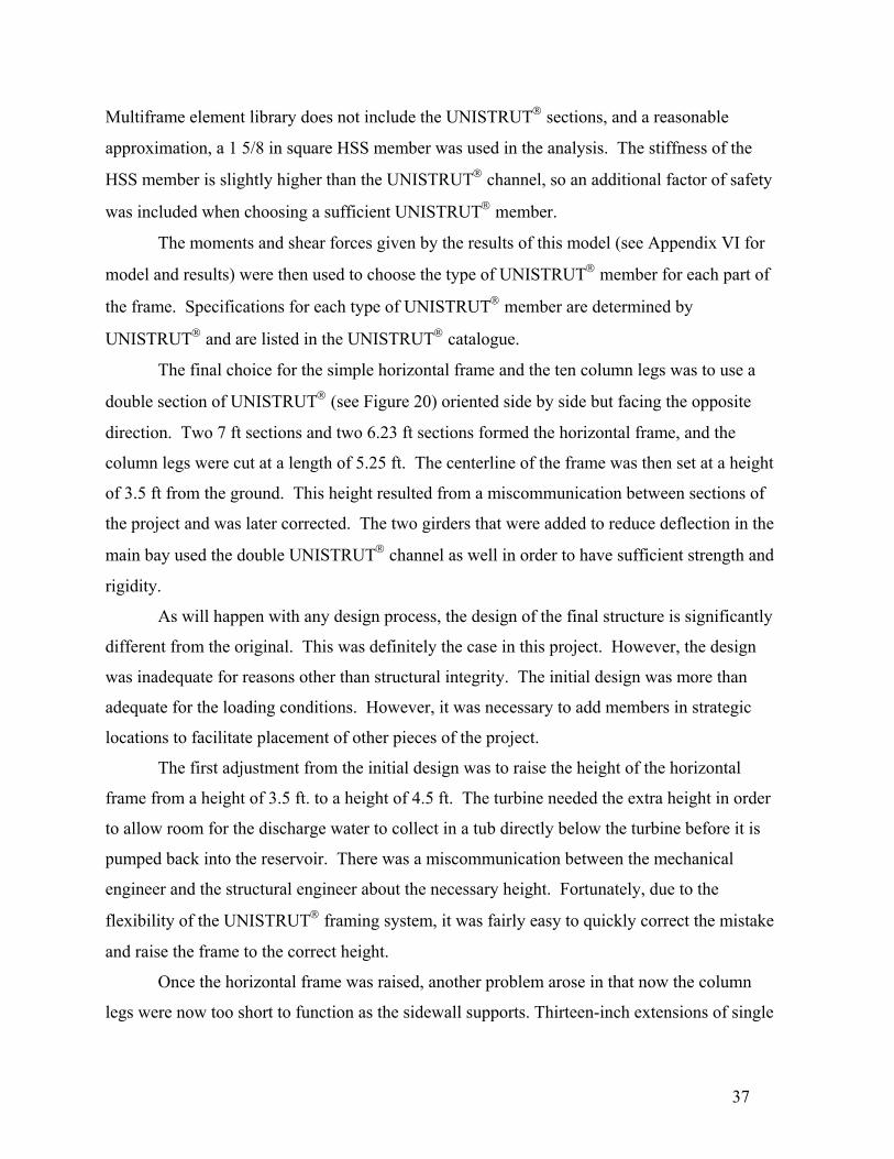
Once the horizontal frame was raised, another problem arose in that now the column

legs were now too short to function as the sidewall supports. Thirteen-inch extensions of single

38

channel UNISTRUT® were added to the existing column legs in order to compensate for this

problem (see Figure 21). On the 6.5 ft section of the reservoir wall, two extensions of 2 ft had

to be added to either side of the single column leg in order to obtain sufficient support.

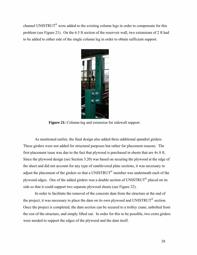
As mentioned earlier, the final design also added three additional spandrel girders.

These girders were not added for structural purposes but rather for placement reasons. The

first placement issue was due to the fact that plywood is purchased in sheets that are 4x 8 ft.

Since the plywood design (see Section 3.20) was based on securing the plywood at the edge of

the sheet and did not account for any type of cantilevered plate sections, it was necessary to

adjust the placement of the girders so that a UNISTRUT® member was underneath each of the

plywood edges. One of the added girders was a double section of UNISTRUT® placed on its

side so that it could support two separate plywood sheets (see Figure 22).

In order to facilitate the removal of the concrete dam from the structure at the end of

the project, it was necessary to place the dam on its own plywood and UNISTRUT® section.

Once the project is completed, the dam section can be secured to a trolley crane, unbolted from

the rest of the structure, and simply lifted out. In order for this to be possible, two extra girders

were needed to support the edges of the plywood and the dam itself.

Figure 21: Column-leg and extension for sidewall support.

39

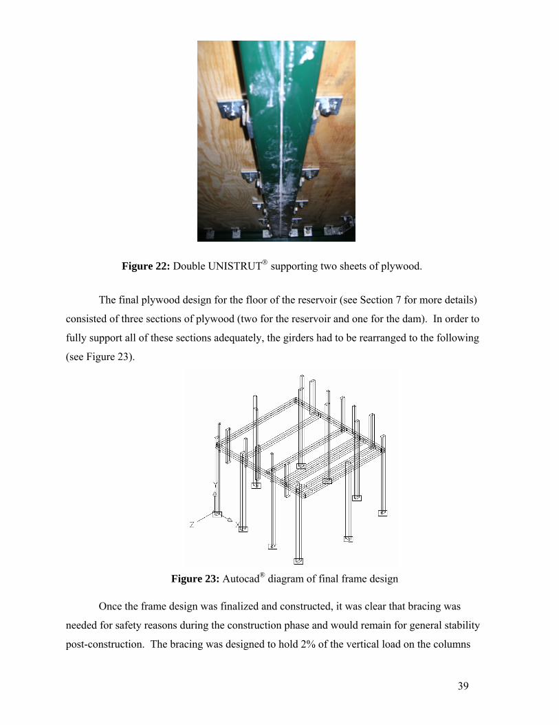
The final plywood design for the floor of the reservoir (see Section 7 for more details)

consisted of three sections of plywood (two for the reservoir and one for the dam). In order to

fully support all of these sections adequately, the girders had to be rearranged to the following

(see Figure 23).

Once the frame design was finalized and constructed, it was clear that bracing was

needed for safety reasons during the construction phase and would remain for general stability

post-construction. The bracing was designed to hold 2% of the vertical load on the columns

Figure 22: Double UNISTRUT® supporting two sheets of plywood.

Figure 23: Autocad® diagram of final frame design

40

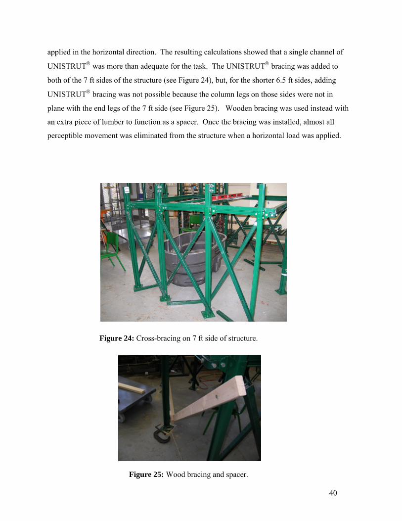
applied in the horizontal direction. The resulting calculations showed that a single channel of

UNISTRUT® was more than adequate for the task. The UNISTRUT® bracing was added to

both of the 7 ft sides of the structure (see Figure 24), but, for the shorter 6.5 ft sides, adding

UNISTRUT® bracing was not possible because the column legs on those sides were not in

plane with the end legs of the 7 ft side (see Figure 25). Wooden bracing was used instead with

an extra piece of lumber to function as a spacer. Once the bracing was installed, almost all

perceptible movement was eliminated from the structure when a horizontal load was applied.

Figure 24: Cross-bracing on 7 ft side of structure.

Figure 25: Wood bracing and spacer.

41

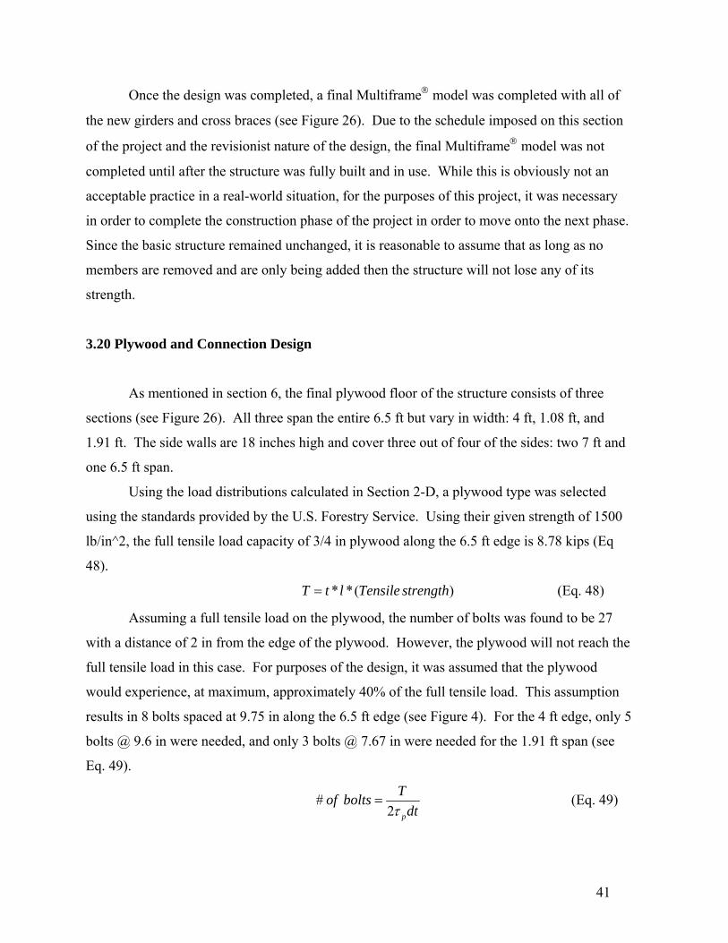
Once the design was completed, a final Multiframe® model was completed with all of

the new girders and cross braces (see Figure 26). Due to the schedule imposed on this section

of the project and the revisionist nature of the design, the final Multiframe® model was not

completed until after the structure was fully built and in use. While this is obviously not an

acceptable practice in a real-world situation, for the purposes of this project, it was necessary

in order to complete the construction phase of the project in order to move onto the next phase.

Since the basic structure remained unchanged, it is reasonable to assume that as long as no

members are removed and are only being added then the structure will not lose any of its

strength.

3.20 Plywood and Connection Design

As mentioned in section 6, the final plywood floor of the structure consists of three

sections (see Figure 26). All three span the entire 6.5 ft but vary in width: 4 ft, 1.08 ft, and

1.91 ft. The side walls are 18 inches high and cover three out of four of the sides: two 7 ft and

one 6.5 ft span.

Using the load distributions calculated in Section 2-D, a plywood type was selected

using the standards provided by the U.S. Forestry Service. Using their given strength of 1500

lb/in^2, the full tensile load capacity of 3/4 in plywood along the 6.5 ft edge is 8.78 kips (Eq

48).

* *( )T t l Tensile strength= (Eq. 48)

Assuming a full tensile load on the plywood, the number of bolts was found to be 27

with a distance of 2 in from the edge of the plywood. However, the plywood will not reach the

full tensile load in this case. For purposes of the design, it was assumed that the plywood

would experience, at maximum, approximately 40% of the full tensile load. This assumption

results in 8 bolts spaced at 9.75 in along the 6.5 ft edge (see Figure 4). For the 4 ft edge, only 5

bolts @ 9.6 in were needed, and only 3 bolts @ 7.67 in were needed for the 1.91 ft span (see

Eq. 49).

#2 p

Tof boltsdtτ

= (Eq. 49)

42

The numbers and spacing of the bolts is based upon the shearing strength of the

plywood. Pull out Shearing failure is one of two possible failure modes of the plywood-

UNISTRUT® connection. The second failure mode is punching shear failure (see Eq. 50).

In this specific loading case, the shear failure is the controlling mode.

# * * tof bolts D t τ= (Eq. 50)

In order to fully understand the behavior of the plywood under the full static load of the

water and concrete, a plate model was developed and run in ANSYS. This model also

identified the highest concentrations of stress under loading for the plywood, which confirmed

the proper placement of the UNISTRUT® girders and number of connections. The ANSYS

model is based upon a Shell 63 element in the ANSYS library. It is a simple 4-node element

that can be used when modeling a 2-D plate. In order to create the model, each bay of the

frame must be modeled as a separate element.

The original ANSYS model was created based on the initial design of two girders

crossing the main bay of the frame. Therefore, there should be three separate elements in the

model. However, in order to include the correct loading, separate elements had to be created

for the dam sections and the water sections, so the final model has four elements. Once an

element is created and its physical properties are defined, it must be meshed before the loads

can be defined. Once the distributed loads calculated in Section 2 are defined on the model, it

Figure 26: Top view of plywood floor of reservoir. The lines of bolts crossing the frame define the three sections of plywood.

43

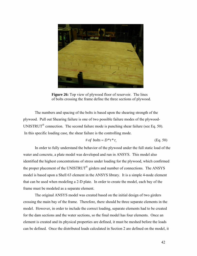
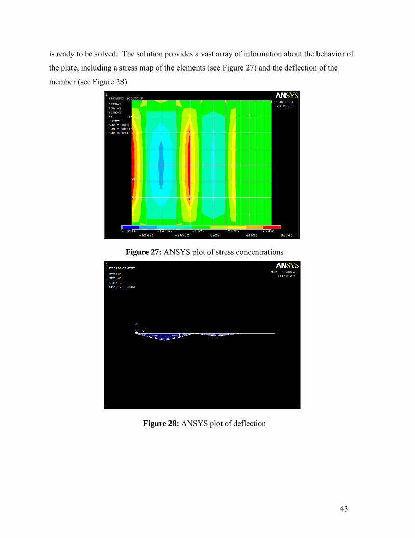
is ready to be solved. The solution provides a vast array of information about the behavior of

the plate, including a stress map of the elements (see Figure 27) and the deflection of the

member (see Figure 28).

Figure 27: ANSYS plot of stress concentrations

Figure 28: ANSYS plot of deflection

44

3.21 Turbine Parameter Selection and Construction

From the expected head and volume flow of the water coming from the dam, the length

and curvature of the blades as well as the diameter of the endplates can be determined using

the equations derived in the previous section. Because, the blades are to be manufactured out

of sections of pipe, the radius of curvature is fixed depending on the pipe size. The endplate

diameter, runner length and the turbine’s rotational speed can then be calculated based on this

curvature. The endplate diameter is calculated from equation (46) and the fact that 1 12r D= .

Once 1D is known, the rotational speed can be calculated from equation (27) and the Runner

length can be calculated from equation (30). (In general, 1 inch is added to the runner length to

in order to give sufficient clearance between the nozzle and the endplates)

Table 3: Pipe Size Selection

Nominal Pipe

Size I.D.

Runner Radius of

Curvature

Endplate

Diameter RPM

Runner

Length

1/2 0.662 0.331 2.03 794 10.53

3/4 0.824 0.412 2.53 638 8.66

1 1.049 0.5245 3.22 501 7.02

1 1/4 1.38 0.69 4.23 381 5.57

1 1/2 1.61 0.805 4.94 327 4.92

2 2.067 1.0335 6.34 254 4.05

2 1/2 2.469 1.2345 7.57 213 3.56

3 3.068 1.534 9.41 171 3.06

4 4.026 2.013 12.35 131 2.57

6 6.065 3.0325 18.60 87 2.04

Overall, Mockmore and Marryfield found that the crossflow turbine was most efficient

between 200 and 300 RPMs. Therefore, the nominal pipe size of 2 inches was selected for this

project. This pipe was then cut into sections of the appropriate length and a milling machine

was used to cut appropriate size cords of the pipe for the blades. Two endplates were also

made by trimming pieces of stock aluminum on the lath until they were the appropriate size.

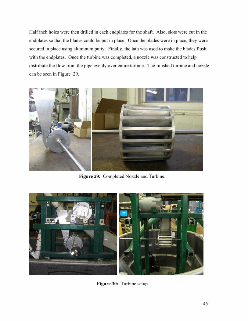
45

Half inch holes were then drilled in each endplates for the shaft. Also, slots were cut in the

endplates so that the blades could be put in place. Once the blades were in place, they were

secured in place using aluminum putty. Finally, the lath was used to make the blades flush

with the endplates. Once the turbine was completed, a nozzle was constructed to help

distribute the flow from the pipe evenly over entire turbine. The finished turbine and nozzle

can be seen in Figure 29.

Figure 29: Completed Nozzle and Turbine.

Figure 30: Turbine setup

46

3.26 Turbine Setup

The turbine setup was done using a UNISTRUT® frame. The frame consisted of four

legs which were held in place with 6 cross members. As can be seen in Figure 30, the nozzle is

supported by two UNISTRUT® cross members. Each of the tabs of the nozzle rests on one of

the cross members and bolts hold the nozzle in place. A pipe from the dam connects to the top

of the nozzle through an expansion into a larger piece of tubing. This tubing is then fit to the

shape of the nozzle in order to make the transition from the pipe to the nozzle as smooth as

possible.

The turbine itself rests on two other UNISTRUT® pieces. Each end of the shaft that

connects to the turbine is set in ball barring which are bolted into the UNISTRUT® frame. The

shaft is then connected to the generator through a timing belt which is used to transfer

mechanical energy from the turbine to the generator. A timing belt was selected because the

teeth in the belt and the pulleys allow relatively low tension to be used in the belt. This makes

the belt system much easier to setup and run. A pulley ratio of 24:7 was used in order to step

the speed of the turbine up to the required speed for the motor to run effectively.

The motor was set on two pieces of UNISTRUT® and bolted into UNISTRUT®

connectors. These connectors were then bolted onto two other pieces of UNISTRUT®. This

setup was necessary to prevent the motor from shaking during operation. Instead, the stand

effectively absorbed the motor vibrations and allowed the motor and belt system to run

smoothly and effectively.

The motor itself is a shunt wound motor that runs at around 525 RPM. This motor was

selected because it runs at low speeds and because it has variable field strength. It was

important to select a motor that runs at low speeds because the turbine runs between 150 and

350 RPM. Therefore, in order to avoid an extremely large gear ratio in the belt system a low

speed motor was needed. Also, it was important that the field strength on the motor could be

varied because this allowed the speed of the turbine to be varied while keeping the head

constant. Therefore, the optimal speed of the turbine at each head could be determined.

47

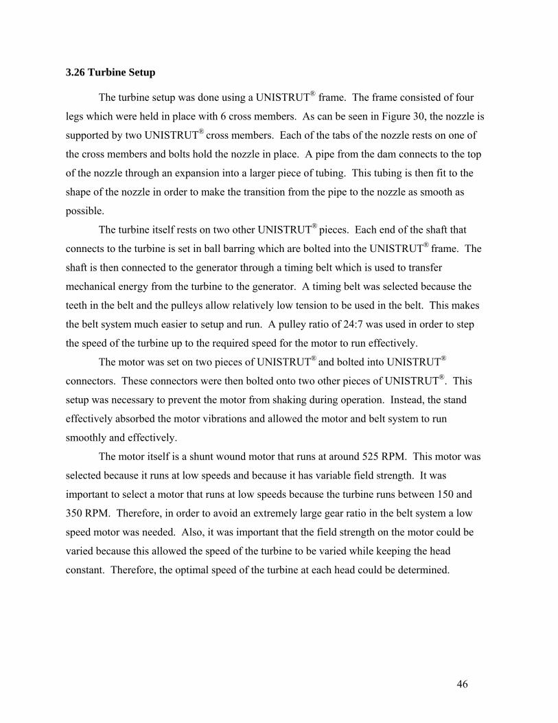
Figure 31: Turbine Operation

Overall, the turbine operated very smoothly. Almost all of the water from the nozzle

ended up flowing through the turbine and transferring its energy to the turbine. This is the

result of the close fit between the nozzle and the turbine. The nozzle was curved so that the

entrance of the water onto the turbine equaled the angle of the blade at the entrance point.

Also, a semicircular section of the nozzle was cutout so that the turbine could fit in close to the

nozzle. There was some leakage at the top of the nozzle. However, this loss was negligible

compared to the amount of water that actually flowed through the turbine.

3.27 Stepped Spillway Stepped spillways are a becoming an ever popular way for handling flood releases in

RCC dams because they are simple and economical to build. RCC dams are laid in lifts;

therefore, steps already exist on the downstream face of the dam. This means that the steps

just need a thin layer of conventional concrete to be added to protect the dam against erosion

and the stepped spillway is basically ready. The stepped spillway also dissipates significant

amounts of energy as the water travels down it. Energy dissipation in the spillway is important

for a couple of different reasons. First of all, energy dissipation along the spillway can help

reduce downstream erosion. Energy dissipation in the spillway also reduces the amount of

energy dissipation that needs to occur at the toe of the dam. Therefore, this energy dissipation

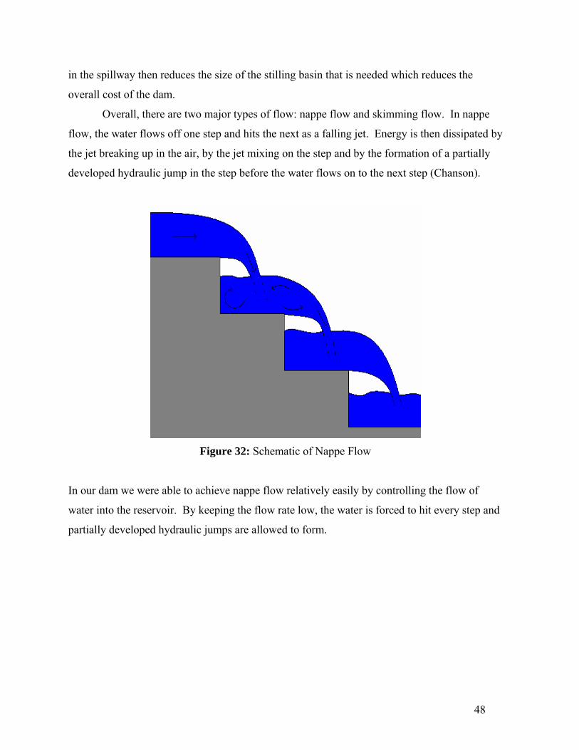
48

in the spillway then reduces the size of the stilling basin that is needed which reduces the

overall cost of the dam.

Overall, there are two major types of flow: nappe flow and skimming flow. In nappe

flow, the water flows off one step and hits the next as a falling jet. Energy is then dissipated by

the jet breaking up in the air, by the jet mixing on the step and by the formation of a partially

developed hydraulic jump in the step before the water flows on to the next step (Chanson).

Figure 32: Schematic of Nappe Flow

In our dam we were able to achieve nappe flow relatively easily by controlling the flow of

water into the reservoir. By keeping the flow rate low, the water is forced to hit every step and

partially developed hydraulic jumps are allowed to form.

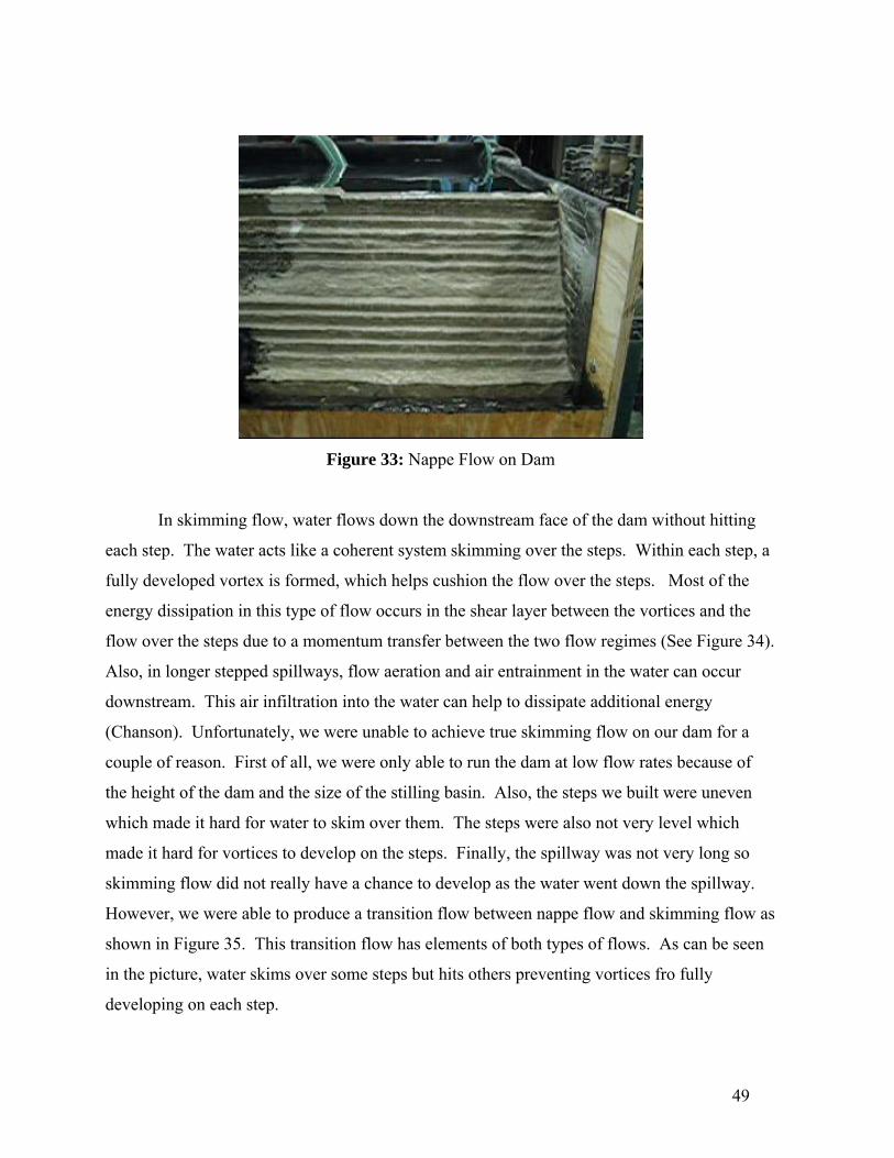
49

Figure 33: Nappe Flow on Dam

In skimming flow, water flows down the downstream face of the dam without hitting

each step. The water acts like a coherent system skimming over the steps. Within each step, a

fully developed vortex is formed, which helps cushion the flow over the steps. Most of the

energy dissipation in this type of flow occurs in the shear layer between the vortices and the

flow over the steps due to a momentum transfer between the two flow regimes (See Figure 34).

Also, in longer stepped spillways, flow aeration and air entrainment in the water can occur

downstream. This air infiltration into the water can help to dissipate additional energy

(Chanson). Unfortunately, we were unable to achieve true skimming flow on our dam for a

couple of reason. First of all, we were only able to run the dam at low flow rates because of

the height of the dam and the size of the stilling basin. Also, the steps we built were uneven

which made it hard for water to skim over them. The steps were also not very level which

made it hard for vortices to develop on the steps. Finally, the spillway was not very long so

skimming flow did not really have a chance to develop as the water went down the spillway.

However, we were able to produce a transition flow between nappe flow and skimming flow as

shown in Figure 35. This transition flow has elements of both types of flows. As can be seen

in the picture, water skims over some steps but hits others preventing vortices fro fully

developing on each step.

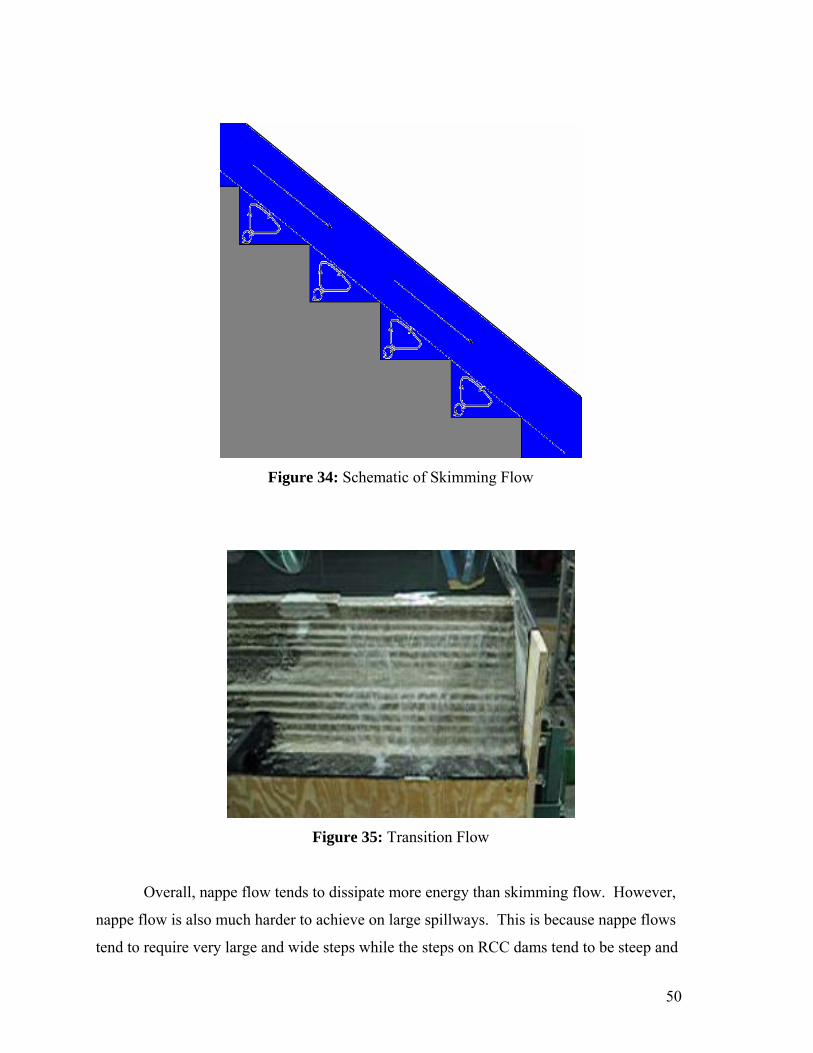
50

Figure 34: Schematic of Skimming Flow

Figure 35: Transition Flow

Overall, nappe flow tends to dissipate more energy than skimming flow. However,

nappe flow is also much harder to achieve on large spillways. This is because nappe flows

tend to require very large and wide steps while the steps on RCC dams tend to be steep and

51

narrow. Also, nappe flows require relatively low flow rates, therefore nappe flows can not be

achieved in large release that are usually required for flood control. This means that skimming

flow is the much more common flow regime on large stepped spillways.

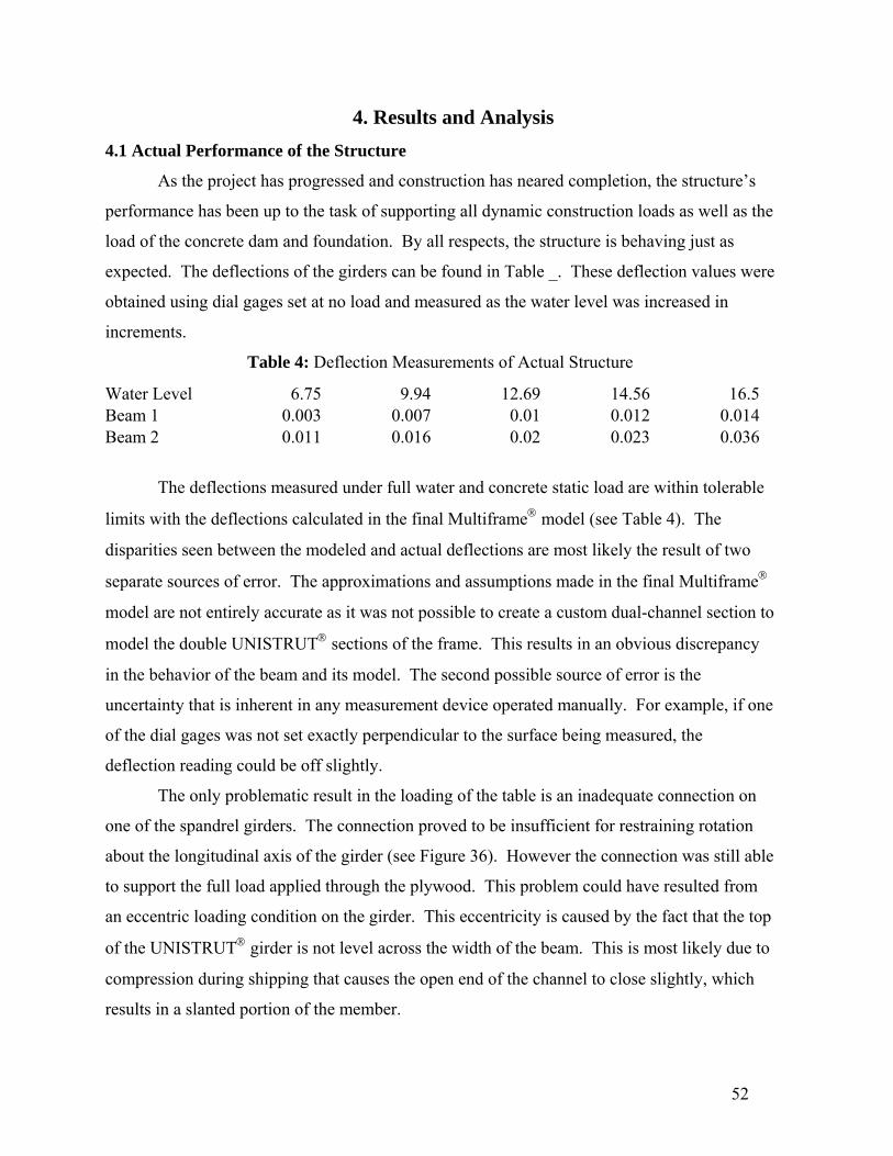
52

4. Results and Analysis 4.1 Actual Performance of the Structure

As the project has progressed and construction has neared completion, the structure’s

performance has been up to the task of supporting all dynamic construction loads as well as the

load of the concrete dam and foundation. By all respects, the structure is behaving just as

expected. The deflections of the girders can be found in Table _. These deflection values were

obtained using dial gages set at no load and measured as the water level was increased in

increments.

Table 4: Deflection Measurements of Actual Structure

Water Level 6.75 9.94 12.69 14.56 16.5Beam 1 0.003 0.007 0.01 0.012 0.014Beam 2 0.011 0.016 0.02 0.023 0.036

The deflections measured under full water and concrete static load are within tolerable

limits with the deflections calculated in the final Multiframe® model (see Table 4). The

disparities seen between the modeled and actual deflections are most likely the result of two

separate sources of error. The approximations and assumptions made in the final Multiframe®

model are not entirely accurate as it was not possible to create a custom dual-channel section to

model the double UNISTRUT® sections of the frame. This results in an obvious discrepancy

in the behavior of the beam and its model. The second possible source of error is the

uncertainty that is inherent in any measurement device operated manually. For example, if one

of the dial gages was not set exactly perpendicular to the surface being measured, the

deflection reading could be off slightly.

The only problematic result in the loading of the table is an inadequate connection on

one of the spandrel girders. The connection proved to be insufficient for restraining rotation

about the longitudinal axis of the girder (see Figure 36). However the connection was still able

to support the full load applied through the plywood. This problem could have resulted from

an eccentric loading condition on the girder. This eccentricity is caused by the fact that the top

of the UNISTRUT® girder is not level across the width of the beam. This is most likely due to

compression during shipping that causes the open end of the channel to close slightly, which

results in a slanted portion of the member.

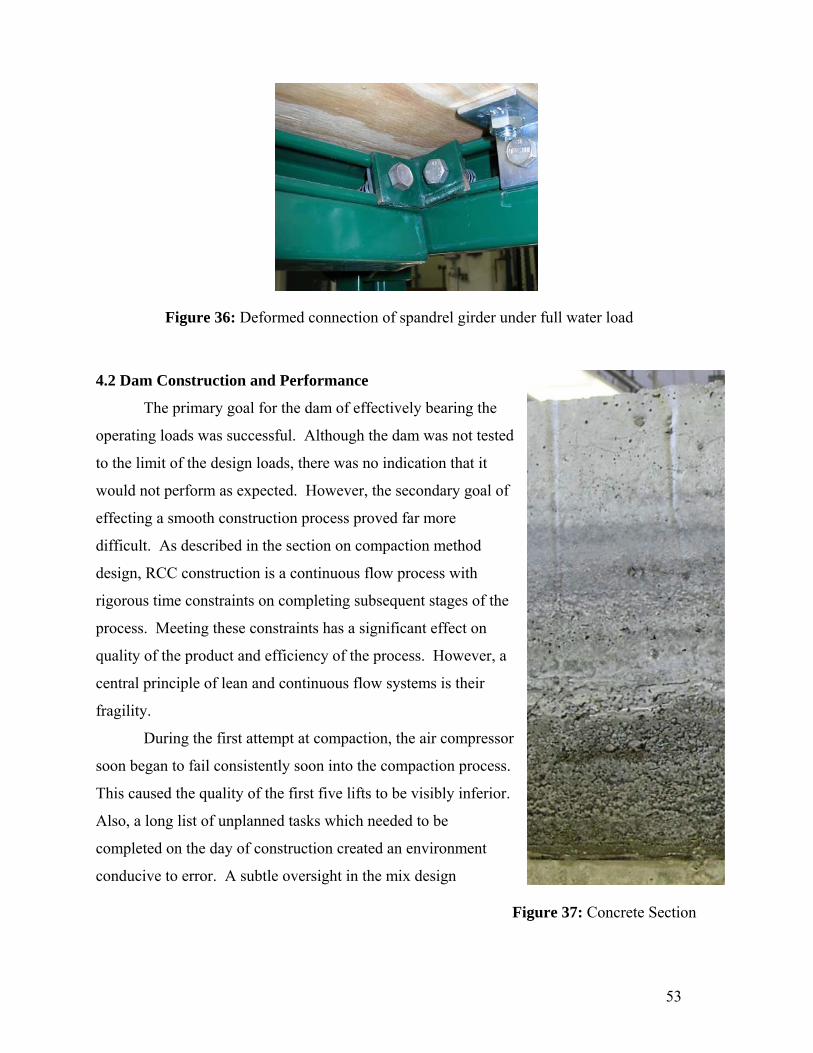
53

4.2 Dam Construction and Performance

The primary goal for the dam of effectively bearing the

operating loads was successful. Although the dam was not tested

to the limit of the design loads, there was no indication that it

would not perform as expected. However, the secondary goal of

effecting a smooth construction process proved far more

difficult. As described in the section on compaction method

design, RCC construction is a continuous flow process with

rigorous time constraints on completing subsequent stages of the

process. Meeting these constraints has a significant effect on

quality of the product and efficiency of the process. However, a

central principle of lean and continuous flow systems is their

fragility.

During the first attempt at compaction, the air compressor

soon began to fail consistently soon into the compaction process.

This caused the quality of the first five lifts to be visibly inferior.

Also, a long list of unplanned tasks which needed to be

completed on the day of construction created an environment

conducive to error. A subtle oversight in the mix design

Figure 36: Deformed connection of spandrel girder under full water load

Figure 37: Concrete Section

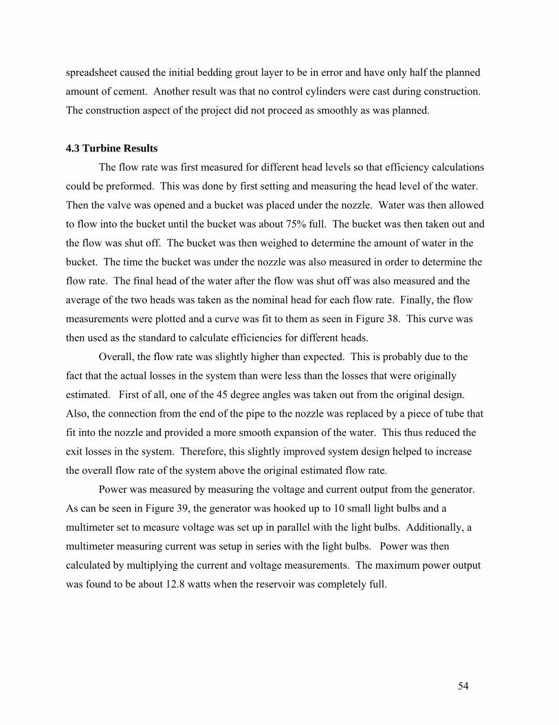
54

spreadsheet caused the initial bedding grout layer to be in error and have only half the planned

amount of cement. Another result was that no control cylinders were cast during construction.

The construction aspect of the project did not proceed as smoothly as was planned.

4.3 Turbine Results

The flow rate was first measured for different head levels so that efficiency calculations

could be preformed. This was done by first setting and measuring the head level of the water.

Then the valve was opened and a bucket was placed under the nozzle. Water was then allowed

to flow into the bucket until the bucket was about 75% full. The bucket was then taken out and

the flow was shut off. The bucket was then weighed to determine the amount of water in the

bucket. The time the bucket was under the nozzle was also measured in order to determine the

flow rate. The final head of the water after the flow was shut off was also measured and the

average of the two heads was taken as the nominal head for each flow rate. Finally, the flow

measurements were plotted and a curve was fit to them as seen in Figure 38. This curve was

then used as the standard to calculate efficiencies for different heads.

Overall, the flow rate was slightly higher than expected. This is probably due to the

fact that the actual losses in the system than were less than the losses that were originally

estimated. First of all, one of the 45 degree angles was taken out from the original design.

Also, the connection from the end of the pipe to the nozzle was replaced by a piece of tube that

fit into the nozzle and provided a more smooth expansion of the water. This thus reduced the

exit losses in the system. Therefore, this slightly improved system design helped to increase

the overall flow rate of the system above the original estimated flow rate.

Power was measured by measuring the voltage and current output from the generator.

As can be seen in Figure 39, the generator was hooked up to 10 small light bulbs and a

multimeter set to measure voltage was set up in parallel with the light bulbs. Additionally, a

multimeter measuring current was setup in series with the light bulbs. Power was then

calculated by multiplying the current and voltage measurements. The maximum power output

was found to be about 12.8 watts when the reservoir was completely full.

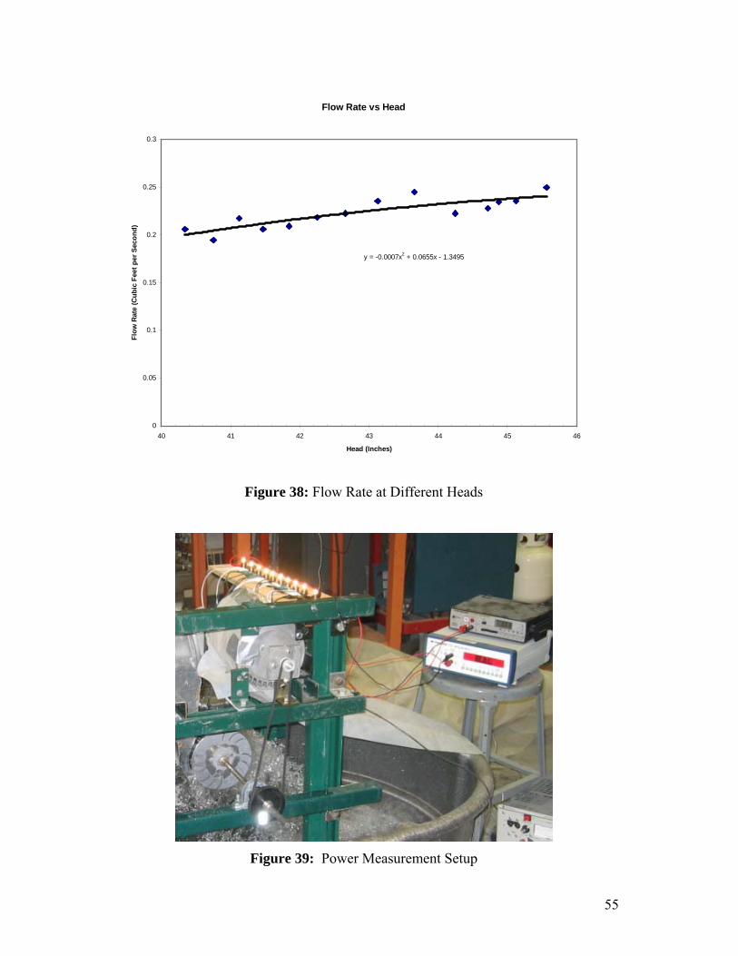
55

Flow Rate vs Head

y = -0.0007x2 + 0.0655x - 1.3495

0

0.05

0.1

0.15

0.2

0.25

0.3

40 41 42 43 44 45 46

Head (Inches)

Flow

Rat

e (C

ubic

Fee

t per

Sec

ond)

Figure 38: Flow Rate at Different Heads

Figure 39: Power Measurement Setup

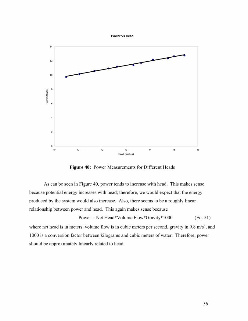
56

Power vs Head

0

2

4

6

8

10

12

14

40 41 42 43 44 45 46

Head (Inches)

Pow

er (W

atts

)

Figure 40: Power Measurements for Different Heads

As can be seen in Figure 40, power tends to increase with head. This makes sense

because potential energy increases with head; therefore, we would expect that the energy

produced by the system would also increase. Also, there seems to be a roughly linear

relationship between power and head. This again makes sense because

Power = Net Head*Volume Flow*Gravity*1000 (Eq. 51)

where net head is in meters, volume flow is in cubic meters per second, gravity in 9.8 m/s2, and

1000 is a conversion factor between kilograms and cubic meters of water. Therefore, power

should be approximately linearly related to head.

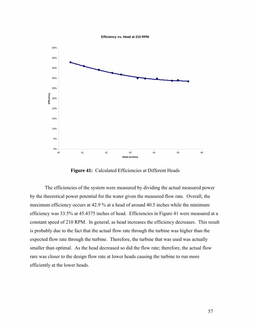
57

Efficiency vs. Head at 210 RPM

0%

5%

10%

15%

20%

25%

30%

35%

40%

45%

50%

40 41 42 43 44 45 46

Head (inches)

Effic

ienc

y

Figure 41: Calculated Efficiencies at Different Heads

The efficiencies of the system were measured by dividing the actual measured power

by the theoretical power potential for the water given the measured flow rate. Overall, the

maximum efficiency occurs at 42.9 % at a head of around 40.5 inches while the minimum

efficiency was 33.5% at 45.4375 inches of head. Efficiencies in Figure 41 were measured at a

constant speed of 210 RPM. In general, as head increases the efficiency decreases. This result

is probably due to the fact that the actual flow rate through the turbine was higher than the

expected flow rate through the turbine. Therefore, the turbine that was used was actually

smaller than optimal. As the head decreased so did the flow rate; therefore, the actual flow

rare was closer to the design flow rate at lower heads causing the turbine to run more

efficiently at the lower heads.

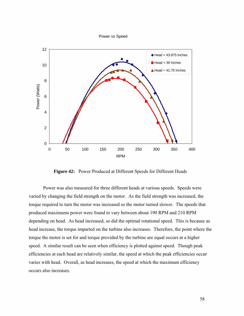
58

Power vs Speed

0

2

4

6

8

10

12

0 50 100 150 200 250 300 350 400

RPM

Pow

er (W

atts

)

Head = 43.875 Inches

Head = 39 Inches

Head = 41.75 Inches

Figure 42: Power Produced at Different Speeds for Different Heads

Power was also measured for three different heads at various speeds. Speeds were

varied by changing the field strength on the motor. As the field strength was increased, the

torque required to turn the motor was increased so the motor turned slower. The speeds that

produced maximums power were found to vary between about 190 RPM and 210 RPM

depending on head. As head increased, so did the optimal rotational speed. This is because as

head increase, the torque imparted on the turbine also increases. Therefore, the point where the

torque the motor is set for and torque provided by the turbine are equal occurs at a higher

speed. A similar result can be seen when efficiency is plotted against speed. Though peak

efficiencies at each head are relatively similar, the speed at which the peak efficiencies occur

varies with head. Overall, as head increases, the speed at which the maximum efficiency

occurs also increases.

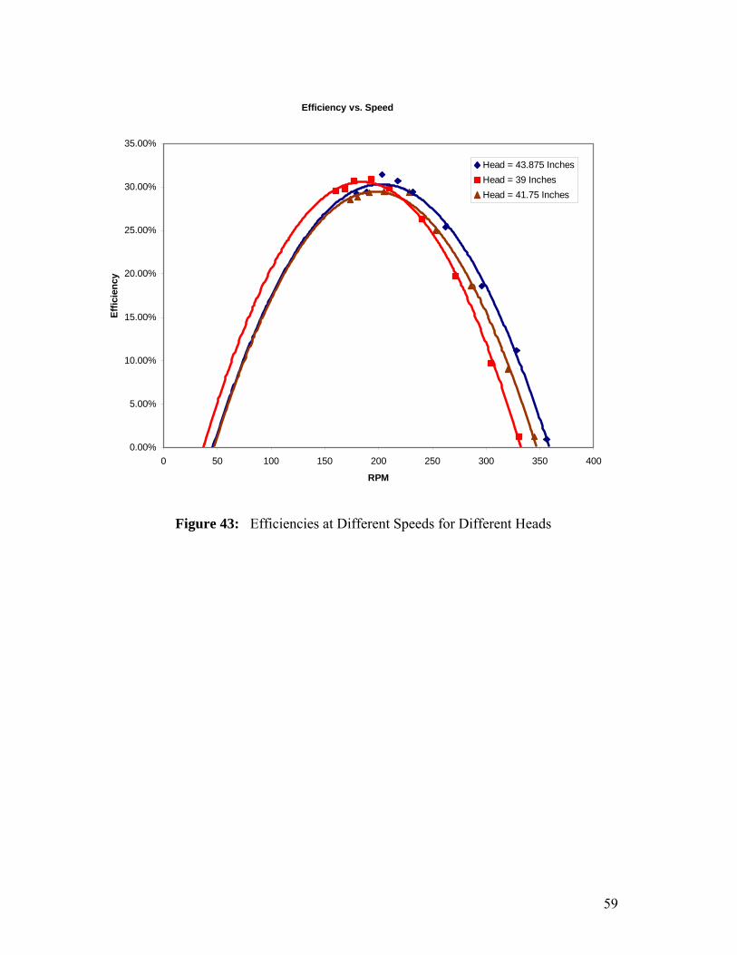
59

Efficiency vs. Speed

0.00%

5.00%

10.00%

15.00%

20.00%

25.00%

30.00%

35.00%

0 50 100 150 200 250 300 350 400

RPM

Effic

ienc

y

Head = 43.875 InchesHead = 39 InchesHead = 41.75 Inches

Figure 43: Efficiencies at Different Speeds for Different Heads

60

5. Conclusions The process of following a project from conception through design and construction

offers many insights into the engineering design process and the level of detail necessary for a

successful design. One of the most important lessons is the importance of continuous, clear

communication between all parties involved in the project. This seems to be an easy objective,

but it quickly becomes complicated as the level of detail increases in the project. Multiple

setbacks in this project were the direct result of poor communication within the team.

The importance of flexibility in a design was very clear as the project progressed. It is

even more important when the level of experience is low, as it is impossible to predict some of

the obstacles that arise in design from reading a textbook. The use of the UNISTRUT framing

system proved to be invaluable for its flexibility to adjust as the design changed and evolved

over the course of the semester. If welded steel or aluminum had been used, it would have

been almost impossible to complete the project in the same amount of time, if at all.

The ability to model complex frames and 3-D models in Multiframe and ANSYS is

another invaluable skill gained from the completion of this project. Those two programs are

such powerful tools to aid in the design process.

Difficulties encountered in the dam casting process emphasized to the students that

extensive preparations must be made before a large continuous flow process is begun. Such

processes are fragile and demanding, and time invested up front is sure to pay off in a simpler

and stabler process.

Also, the importance and difficulty of estimating the time requirements for complex

projects must be considered. The scope of large engineering projects will necessarily test the

boundaries of the engineer’s area of expertise. This makes time estimates and project planning

more crucial and more difficult at the same time.

61

6. References ACI Committee 207. Roller-Compacted Mass Concrete. ACI 207.5R-99. American Concrete

Institute, 1999. American Society for Testing and Materials. ASTM Standard C1245, C1176, C1435, C470. Breslin, W.R. Small Michell (Banki) Turbine: A Construction Manual. Volunteers In Technical Assistance. Arlington, Virginia: 1980. Chanson, Hubert. “Stepped Spillway and Air Entrainment.” Canadian Journal of Civil Engineering, Volume 20. June 1993. pp. 422-435. Dolen, Timothy (Interview). USBR Materials Engineering and Research Laboratory, Research Civil Engineer, Technical Specialist. 2-28, 2006. Fraenkel, Paish, Bokalders, Harvey, Brown, Edwards “Micro-hydro power, A Guide for Development Workers.” Intermediate Technology Publications. London: 1997. Hansen, Kenneth D.; Reinhardt, William G. Roller-Compacted Concrete Dams. USA,

McGraw-Hill, 1991. Hunsaker, J.C., and B.G. Rightmire. Engineering Applications of Fluid Mechanics. McGraw-Hill. New York: 1947. Japikse, David and Nicholas C. Baines. Introduction to Turbomachinery. Concepts ETI. New York: 1997. Kurita, Morio; Aoyagi, Yukio; Endo, Takao; Okumura, Tadahiko. “Compaction Characteristics of Roller Compacted Concrete.” Roller Compacted Concrete II. American Society of Civil Engineers, CA, 1988. Lyon-Allen, Mary. “Developing a Small Hydroelectric Dam Potential.” Community Service Administration. Washington D.C.: 1979. Mabry, Richard (Interview). Geotechnical Design Engineer, URS Griner. Febuary 24, 2006. Munson, Bruce R., Donald F. Young, and Theodore H. Okiishi. Fundamentals of Fluid Mechanics. John Wiley & Sons. Hoboken, NJ: 2002. Mockmore, C.A., and Fred Marryfield. “The Banki Water Turbine.” Bulletin #25. Engineering Experiment station, Oregon State College. Corvallis, Oregon. February 1949. Poulos, H.G.; Davis, E.H. Elastic solutions for soil and rock mechanics. New York, Wiley, 1974.

62

Prandtl, Ludwig. Essentials of Fluid Dynamics. Hafner Publishing. New York: 1952. Streeter, Victor L., and E. Benjamin Wylie, Fluid Mechanics. McGraw-Hill. New York: 19 Siddiqui, Faruq (Interviews). Swarthmore College, Department of Engineering. Professor. Spring 2003 – Spring 2006 United States Army Corps of Engineers. Roller Compacted Concrete. EM 1110-2-2006. Washington DC, January 2000. www.usace.army.mil/usace-docs/eng-manuals/em1110-2-2006/toc.htm United States Army Corps of Engineers. Gravity Dam Design. EM 1110-2-2200. Washington

DC, June 1995. www.usace.army.mil/usace-docs/eng-manuals/em1110-2-2200/toc.htm

United States Bureau of Reclamation. Design of Gravity Dams. Denver, Colorado, 1976. "Water turbine." Wikipedia, The Free Encyclopedia. 25 Mar 2006, 10:46 UTC. 28 Mar 2006, 02:42 <http://en.wikipedia.org/w/index.php?title=Water_turbine&oldid=45401930>.