Photometric visual servoing for omnidirectional cameras

Guillaume Caron∗ Eric Marchand† El Mustapha Mouaddib‡

Abstract

2D visual servoing consists in using data provided by a vision sensor for controllingthe motions of a dynamic system. Most of visual servoing approaches has relied onthe geometric features that have to be tracked and matched in the image acquiredby the camera. Recent works have highlighted the interest of taking into accountthe photometric information of the entire image. This approach was tackled withimages of perspective cameras. We propose, in this paper, to extend this technique tocentral cameras. This generalization allows to apply this kind of method to catadioptriccameras and wide field of view cameras. Several experiments have been successfullydone with a fisheye camera in order to control a 6 degrees of freedom (dof) robot andwith a catadioptric camera for a mobile robot navigation task.

Autonomous Robots, 2013

1 Introduction

Visual servoing uses the information provided by a vision sensor to control the movements ofa dynamic system ([22, 9, 11]). Considering 2D visual servoing, geometric features are usuallycomputed from image measurements and then, tracked and matched in the images acquiredby the camera. The visual servoing control law allows to move the camera to a referenceposition minimizing the error between desired visual features and their correspondencesdetected in the current image.

Geometric features (points, lines, circles, moments) have been widely used for visualservoing. These features and their different representations can bring interesting propertiesfor the servoing process, such as, when well chosen, a nice decoupling between the cameradegrees of freedom ([8]). However, detecting, tracking and matching image measurementsand the corresponding visual features effectively is still a difficult problem ([26]). To deal withthis issue, it is possible to directly use the image as a whole rather than extract geometricalfeatures. This leads to direct visual servoing scheme ([30, 16, 12, 15, 23]). It withdraws

∗Universite de Picardie Jules Verne, MIS laboratory, Amiens, France Guillaume.Caron@u-picardie.fr†Universite de Rennes 1, IRISA, INRIA Rennes - Bretagne Atlantique, Lagadic marchand@irisa.fr‡Universite de Picardie Jules Verne, MIS laboratory, Amiens, France mouaddib@u-picardie.fr

1

the detection and matching problems and, moreover, allows to consider more informationleading to higher accuracy.

Such idea was initially proposed in [30] and in [16]. These works, although no featureswere extracted from the images, do not directly use the image intensity since an eigenspacedecomposition is performed to reduce the dimensionality of image data. The control is thenperformed in the eigenspace and the related interaction matrix that links the variation of theeigenspace to the camera motion is learnt offline. This learning process has two drawbacks:it has to be done for each new object/scene and requires the acquisition of many images ofthe scene at various camera positions.

Photometric features, i.e. pixel intensities of the entire image, have been proposed todirectly be used as input of the control scheme by [12]. In that case, the goal is to minimizethe error between the current and desired image. The visual feature is nothing but the imageitself. The analytic formulation of the interaction matrix that links the variation of the imageintensity to the camera motion was exhibited in [12]. [6] used also a direct intensity basedvisual servoing approach. A direct tracking process based on the image intensity is consideredto estimate the homography between current and desired image. A control law that uses theparameters of this homography as visual feature is then proposed. An interesting kernel-based approach, which also considers the pixels intensity, has been recently proposed in [23].However, only the translations and the rotation around the optical axis have been considered.

This paper addresses the problem of photometric visual servoing for central omnidirec-tional cameras using image intensity as visual feature. It extends the work of [12] investigat-ing different image representations and models directly induced by omnidirectional vision.Indeed, omnidirectional images can be elevated on the sphere of the unified projection modelfor central cameras ([3]).

Previous works were done on the omnidirectional visual servoing to control robotics arms([33]) as well as mobile robots ([28, 34, 5]).

We propose to formulate the omnidirectional photometric visual servoing on the sphereof this model, which is better adapted to the omnidirectional image geometry and low levelprocessing ([17]). We also considered the image plane representation for a fair comparisonprocess.

Many authors point out the interest of considering a large field of view (catadioptriccamera, non-overlapping cameras...) for mobile robot navigation as ([1, 24, 29]), to cite afew papers about the topic:

• First, omnidirectional view provide a complete view of the camera environment whichincreases thechances of sensing non uniform zones of the environment, photometric visual servo-ing, as introduced in [12], being particularly efficient in these conditions.

• Second, translations have less impact on the acquired images and convergence. Rota-tion of the camera leads to a simple rotation in the image whereas with a perspectivecamera this may lead to a complete lack of shared information. We thus usually havea smaller disparity (distance between the projection of a physical point in the current

2

and desired image) in omnidirectional images, leading to a smaller error between thetwo images, which allows an easier convergence of the control law.

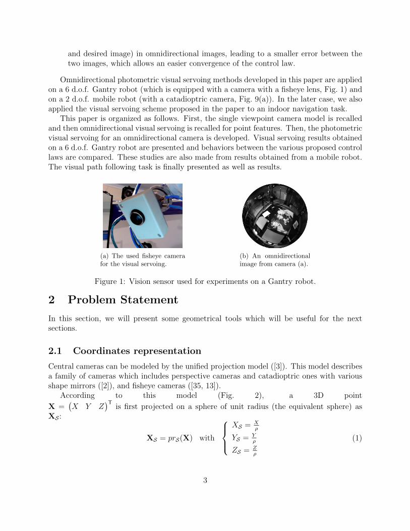
Omnidirectional photometric visual servoing methods developed in this paper are appliedon a 6 d.o.f. Gantry robot (which is equipped with a camera with a fisheye lens, Fig. 1) andon a 2 d.o.f. mobile robot (with a catadioptric camera, Fig. 9(a)). In the later case, we alsoapplied the visual servoing scheme proposed in the paper to an indoor navigation task.

This paper is organized as follows. First, the single viewpoint camera model is recalledand then omnidirectional visual servoing is recalled for point features. Then, the photometricvisual servoing for an omnidirectional camera is developed. Visual servoing results obtainedon a 6 d.o.f. Gantry robot are presented and behaviors between the various proposed controllaws are compared. These studies are also made from results obtained from a mobile robot.The visual path following task is finally presented as well as results.

(a) The used fisheye camerafor the visual servoing.

(b) An omnidirectionalimage from camera (a).

Figure 1: Vision sensor used for experiments on a Gantry robot.

2 Problem Statement

In this section, we will present some geometrical tools which will be useful for the nextsections.

2.1 Coordinates representation

Central cameras can be modeled by the unified projection model ([3]). This model describesa family of cameras which includes perspective cameras and catadioptric ones with variousshape mirrors ([2]), and fisheye cameras ([35, 13]).

According to this model (Fig. 2), a 3D point

X =(X Y Z

)Tis first projected on a sphere of unit radius (the equivalent sphere) as

XS :

XS = prS(X) with

XS = X

ρ

YS = Yρ

ZS = Zρ

(1)

3

where XS =(XS YS ZS

)Tand ρ =

√X2 + Y 2 + Z2.

This parameterization is redundant on a sphere since a coordinate can be written as acombination of others. Hence, two angular coordinates (azimuth and elevation) are sufficient

to represent a point on a sphere S =(φ θ

)Twith:

S =

{φ = arccos(ZS) = arccos(Z / ρ)θ = arctan(YS / XS) = arctan(Y / X)

(2)

The spherical projection is followed by a perspective projection on the image plane (Fig. 2)

as x =(x y 1

)Tby using parameter ξ which depends intrinsically on the omnidirectional

camera type. The final relation between the 3D point and its normalized image point is:x = prξ(X)

with :

x = XSZS+ξ

= XZ+ξρ

= cos(θ) sin(φ)cos(φ)+ξ

y = YSZS+ξ

= YZ+ξρ

= sin(θ) sin(φ)cos(φ)+ξ

(3)

The image point is obtained by:

u =

uv1

=

px 0 u00 py v00 0 1

xy1

= Kx, (4)

where (px, py) are the product of the focal length and horizontal (resp. vertical) size of apixel and (u0, v0) are the principal point coordinates. They are part of the projection modelparameters γ = {px, py, u0, v0, ξ} that are supposed to be known after a calibration process.

The projection function is invertible as pr−1ξ and allows to retrieve the point on the spherecorresponding to x:

XS = pr−1ξ (x) =

ξ+√

1+(1−ξ2)(x2+y2)x2+y2+1

x

ξ+√

1+(1−ξ2)(x2+y2)x2+y2+1

y

ξ+√

1+(1−ξ2)(x2+y2)x2+y2+1

− ξ

. (5)

This equation is used to obtain points coordinates on the unit sphere of the model in Carte-sian representation which can be transformed to the angular representation using equation(2).

As we have seen, the unified model is based on an equivalence sphere as intermediaterepresentation place. This place, will be used to do the visual servoing. Then, we have newpossibilities to model the image and we will be interested in:

1. Cartesian representation x or u (two coordinates) on the 2D image plane

2. Cartesian representation XS (three coordinates) on the 3D equivalence sphere

3. Spherical representation S (two coordinates) on the 3D equivalence sphere

4

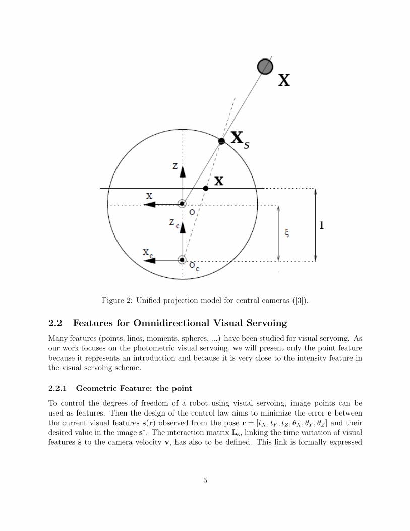
Figure 2: Unified projection model for central cameras ([3]).

2.2 Features for Omnidirectional Visual Servoing

Many features (points, lines, moments, spheres, ...) have been studied for visual servoing. Asour work focuses on the photometric visual servoing, we will present only the point featurebecause it represents an introduction and because it is very close to the intensity feature inthe visual servoing scheme.

2.2.1 Geometric Feature: the point

To control the degrees of freedom of a robot using visual servoing, image points can beused as features. Then the design of the control law aims to minimize the error e betweenthe current visual features s(r) observed from the pose r = [tX , tY , tZ , θX , θY , θZ ] and theirdesired value in the image s∗. The interaction matrix Ls, linking the time variation of visualfeatures s to the camera velocity v, has also to be defined. This link is formally expressed

5

as:s = Lsv (6)

where v =(υ ω

)Tis composed of the linear and angular camera velocities, υ = [υX , υY , υZ ]

andω = [ωX , ωY , ωZ ], respectively. A control law is designed to try to have an exponentialdecoupled decrease of the error e = s(r)− s∗:

v = −λL+s e (7)

with λ a tunable gain to modify the convergence rate and L+s , the pseudo-inverse of a

model of Ls. We mention “a model of Ls” because it cannot be exactly known due tonever perfect knowledge of camera parameters or scene structure. Hence, if a representation(cartesian image plane, cartesian spherical or pure spherical) leads to a better behavior(convergence, residual decrease, camera trajectory), it will mean that this representation isa better modeling of the perfect interaction matrix than others.

2.2.2 Photometric Feature: the intensity

The visual features considered in photometric visual servoing are the luminance of each pointof the image. This approach has already been developed in the case of perspective images.It needs to solve two problems: the interaction matrix and the image gradient.

We consider that the luminance I at a constant pixel location x = (x, y) for all x belongingto the image domain and for a given pose r. Thus, we have:

s(r) = I(r) = (I1, I2, · · · , IN)T (8)

where Ii is the row vector containing pixel intensities of the image line number i. i is varyingfrom 1 to N , the image height. Ii has a size equal to M, the image width. The size of thevector I(r) is equal to N ×M , i.e. the number of image pixels.

We have thus to minimize the difference between current and desired images:

e = I(r)− I∗(r∗), (9)

The control law is then, as in a classical visual servoing scheme, given by:

v = −λL+I (I(r)− I∗(r∗)) (10)

Nevertheless, considering visual servoing as an optimization problem ([25]), [12] formulatephotometric servoing control law using a Levenberg-Marquardt like optimization technique.It has been shown that it ensures better convergence than other kind of control laws. So,instead of using a Gauss-Newton like control law (eq. (7)), this control law is used in thecurrent work:

v = −λ (H + µ diag(H))−1 LTI (I(r)− I∗(r∗)) (11)

6

with H = LTI LI, considering LI is the interaction matrix related to luminance of image I. If

µ is very high this control law behaves like a steepest descent whereas a very low value forµ leads eq. (11) to behave like eq. (10).

As for any pure image based visual servoing approach, only local stability can be obtainedin the photometric visual servoing since redundant visual features are used ([9]). However,as pointed out in the latter reference, this domain is quite large in practice.

2.3 Gradient Computation

As mentioned in the previous section, we need to compute some gradients (geometrical,temporal and image gradient). These gradients depend on the coordinates representationand the used features. Since we will use the equivalence sphere as a work space, we will haveother possibilities and schemes than traditional ones to estimate these gradients.

3 Omnidirectional Photometric Visual Servoing

This section describes three representations for omnidirectional photometric visual servoing:the image plane Cartesian representation, the spherical Cartesian representation and thespherical representation. Photometric visual servoing formulations for each representationare successively proposed and validated in simulation. They are faced in the discussion onsimulation results that ends the section.

3.1 Image Plane Visual Servoing: Cartesian Representation

3.1.1 Interaction Matrix for Geometrical Servoing

When considering points as visual features, i.e.x = (x, y), the interaction matrix Lx, that links the point velocity to the camera veloc-ity v is given by ([9]):

Lx =∂x

∂X

∂X

∂r(12)

For the image plane, the partial derivatives ∂x∂X

are computed from eq. (3) and lead tothe interaction matrix for a point in the omnidirectional image plane.

The second jacobian, ∂X∂r

, is well known for points ([19]) and does not depend on theprojection model which is encapsulated in the first Jacobian. Then, Lx is ([4]):

Lx =(L1 | L2

)(13)

with

L1 =

(−1+x2(1−ξ(α+ξ))+y2

ρ(α+ξ)ξxyρ

αxρ

ξxyρ

−1+y2(1−ξ(α+ξ))+x2ρ(α+ξ)

αyρ

)(14)

7

and

L2 =

(xy − (1+x2)α−ξy2

α+ξy

(1+y2)α−ξx2α+ξ

−xy −x

)(15)

where α =√

1 + (1− ξ2)(x2 + y2) and ρ defined ineq. (3).

3.1.2 Interaction Matrix for Photometric Servoing

The interaction matrix LI(x) formulation is defined under temporal luminance consistancy([12]):

I(x + dx, t+ dt) = I(x, t) (16)

assuming dx is small. If it is small enough, and considering a Lambertian scene, the opticalflow constraint equation (OFCE) is valid ([21]):

∇ITx + It = 0 (17)

with ∇I the spatial gradient of I(x, t) and It = ∂I(x,t)∂t

, is the temporal gradient. Forthe omnidirectional image plane photometric visual servoing (IP-VS), the knowledge of Lx

(a) (b)

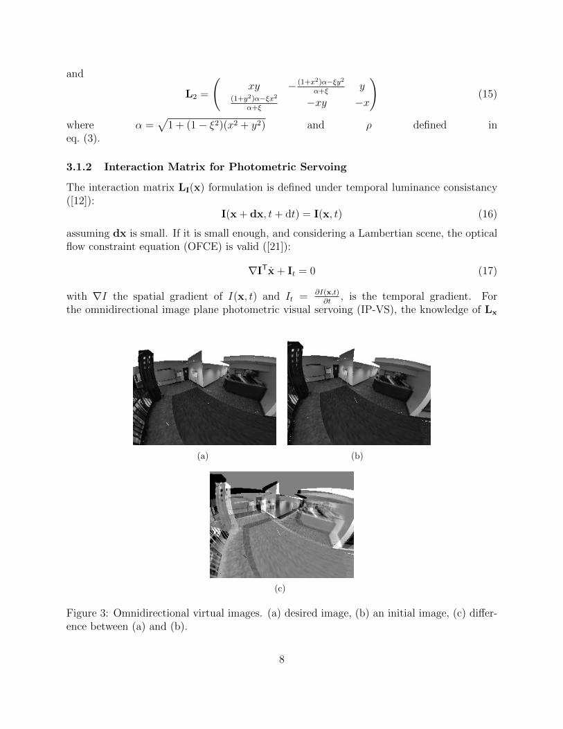
(c)

Figure 3: Omnidirectional virtual images. (a) desired image, (b) an initial image, (c) differ-ence between (a) and (b).

8

(eq. (13)) leads to:It = −∇ITLxv. (18)

And similarly to [12], we get the interaction matrix LI(x) related to I at pixel x:

LI(x) = −∇ITLx, (19)

where Lx is given by eq. (13).

3.1.3 Photometric Gradient Computation

On the image plane and in the case of perspective image, the image gradients ∇I are com-puted using the same neighborhood for all image point: a square regularly sampled. Forinstance, in [12], it is approximated by a convolution of I with two Gaussian derivatives.

In omnidirectional images, we can use the same approach to compute the gradients. But,the image geometry is different, i.e. resolution and orientation are not constant. For thisreason, many works have been done to adapt image processing tools for these images, andfor gradient computation. One of these approaches, consists in adapting the neighborhood([17]). The reader can find more details and a discussion about these technics in ([7]). In thelatter work, no particular impact of adapted image gradients computation was noticeablefor the image plane representation, with convolution window size 7 × 7 as we use. Hence,for the IP-VS, image gradients ∇I were classically computed.

3.1.4 Validation

Validation is done on synthetic views of a real environment from one of the Trakmark(http://trakmark.net) datasets. We made a real-time omnidirectional OpenGL camera us-ing GPU shaders (GLSL language). The projection model of this camera is the unifiedprojection model ([3]). An obtained image is presented in figure 3(a).

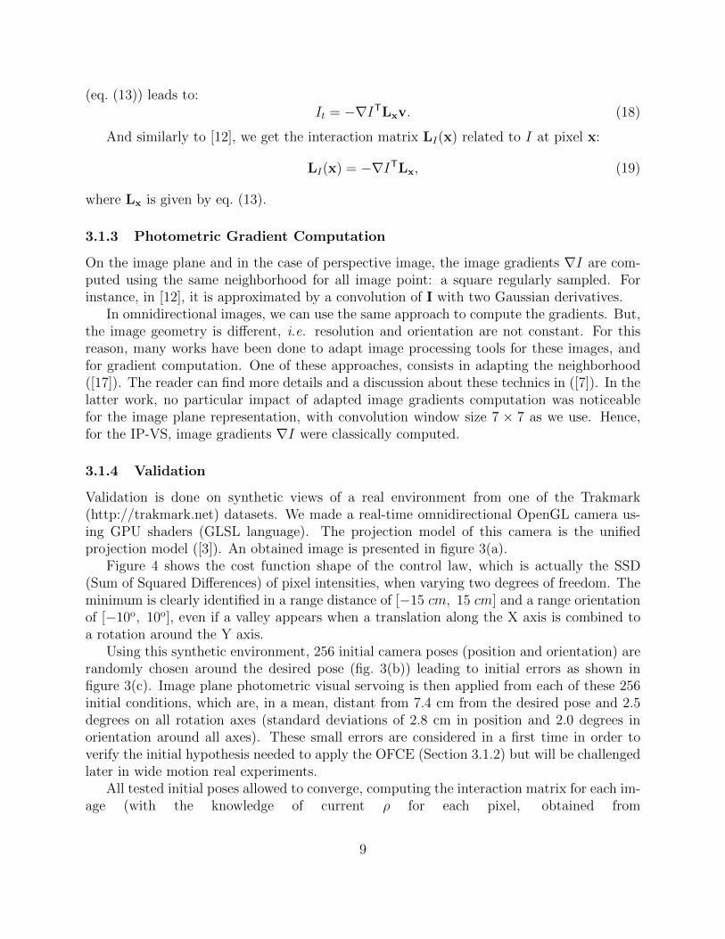
Figure 4 shows the cost function shape of the control law, which is actually the SSD(Sum of Squared Differences) of pixel intensities, when varying two degrees of freedom. Theminimum is clearly identified in a range distance of [−15 cm, 15 cm] and a range orientationof [−10o, 10o], even if a valley appears when a translation along the X axis is combined toa rotation around the Y axis.

Using this synthetic environment, 256 initial camera poses (position and orientation) arerandomly chosen around the desired pose (fig. 3(b)) leading to initial errors as shown infigure 3(c). Image plane photometric visual servoing is then applied from each of these 256initial conditions, which are, in a mean, distant from 7.4 cm from the desired pose and 2.5degrees on all rotation axes (standard deviations of 2.8 cm in position and 2.0 degrees inorientation around all axes). These small errors are considered in a first time in order toverify the initial hypothesis needed to apply the OFCE (Section 3.1.2) but will be challengedlater in wide motion real experiments.

All tested initial poses allowed to converge, computing the interaction matrix for each im-age (with the knowledge of current ρ for each pixel, obtained from

9

(a) (b)

Figure 4: Cost function shape when varying two degrees of freedom: (a) combined translationalong X and Y axes (in meters) and (b) combined translation along the X axis and rotationaround the Y axis of the camera (in meters and degrees).

(a) current IM and known depth (b) current IM and constant depth

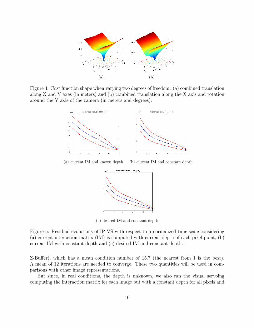
(c) desired IM and constant depth

Figure 5: Residual evolutions of IP-VS with respect to a normalized time scale considering(a) current interaction matrix (IM) is computed with current depth of each pixel point, (b)current IM with constant depth and (c) desired IM and constant depth.

Z-Buffer), which has a mean condition number of 15.7 (the nearest from 1 is the best).A mean of 12 iterations are needed to converge. These two quantities will be used in com-parisons with other image representations.

But since, in real conditions, the depth is unknown, we also ran the visual servoingcomputing the interaction matrix for each image but with a constant depth for all pixels and

10

all images. The ρ value corresponds to the mean of ρ values at the desired pose. 100 % ofthese simulations converged in a mean of 10.3 iterations for a mean conditioning of 21.2.

Finally, the computation (and inversion) of the interaction matrix for each image is abit too long to keep a standard 25 Hz frame rate and, as it is often chosen as a correct ap-proximation, assuming the camera is rather close to its optimal pose, the desired interactionmatrix with a constant depth is finally used, as it will be the case in real experiments. Withthis consideration, still 100 % of tested cases converged in a mean of 10.3 iterations for aninteraction matrix conditioning of 18.8. All these results are summed up in table 1.

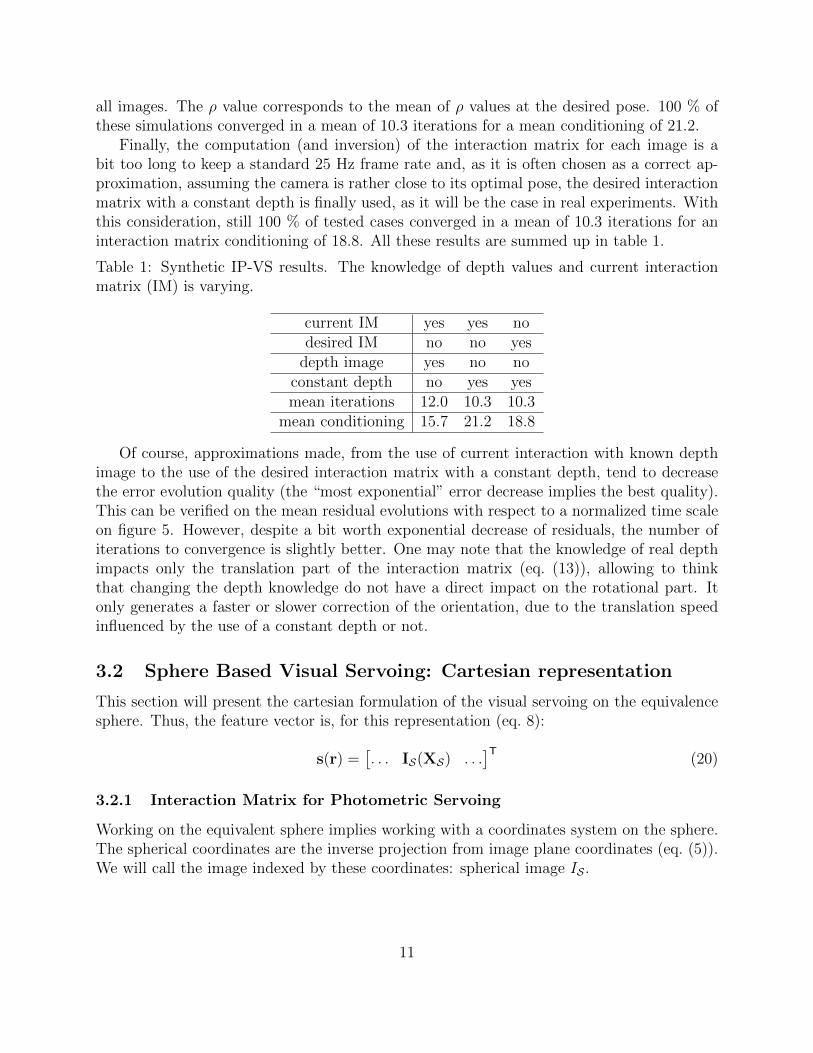
Table 1: Synthetic IP-VS results. The knowledge of depth values and current interactionmatrix (IM) is varying.

current IM yes yes nodesired IM no no yes

depth image yes no noconstant depth no yes yesmean iterations 12.0 10.3 10.3

mean conditioning 15.7 21.2 18.8

Of course, approximations made, from the use of current interaction with known depthimage to the use of the desired interaction matrix with a constant depth, tend to decreasethe error evolution quality (the “most exponential” error decrease implies the best quality).This can be verified on the mean residual evolutions with respect to a normalized time scaleon figure 5. However, despite a bit worth exponential decrease of residuals, the number ofiterations to convergence is slightly better. One may note that the knowledge of real depthimpacts only the translation part of the interaction matrix (eq. (13)), allowing to thinkthat changing the depth knowledge do not have a direct impact on the rotational part. Itonly generates a faster or slower correction of the orientation, due to the translation speedinfluenced by the use of a constant depth or not.

3.2 Sphere Based Visual Servoing: Cartesian representation

This section will present the cartesian formulation of the visual servoing on the equivalencesphere. Thus, the feature vector is, for this representation (eq. 8):

s(r) =[. . . IS(XS) . . .

]T(20)

3.2.1 Interaction Matrix for Photometric Servoing

Working on the equivalent sphere implies working with a coordinates system on the sphere.The spherical coordinates are the inverse projection from image plane coordinates (eq. (5)).We will call the image indexed by these coordinates: spherical image IS .

11

Still under constant illumination assumption(eq. (16)), the OFCE (eq. (17)) is reformulated to fit the cartesian spherical representa-tion:

∇ITS XS + ISt = 0, (21)

detailed as:∂IS∂XS

XS +∂IS∂YS

YS +∂IS∂ZS

ZS + ISt = 0. (22)

The interaction matrix LIS(XS) related to IS at spherical point XS , for cartesian sphericalphotometric visual servoing (CS-VS), is defined by:

LIS(XS) = −∇ITSLXS . (23)

LXS is given by equation (24) but the image gradient on the sphere have yet to be expressed.

3.2.2 Interaction Matrix for Geometric Servoing

This parameterization uses 3-coordinates points XSonto the equivalent sphere as defined in equation (1). The interaction matrix LXS hasbeen defined by ([20]), in a different purpose:

LXS =∂XS∂X

∂X

∂r=(1ρ(XSX

TS − I3) [XS ]×

)3×6 . (24)

3.2.3 Photometric Gradient Computation

To approximate the image gradient on the sphere, we estimate ∂IS∂XS

, ∂IS∂YS

and ∂IS∂ZS

by usinga finite difference. We need to chose values for ∆XS , ∆YS and ∆ZS and to interpolate thevalues of the intensity at this point. To compute gradients ( ∂IS

∂XS, ∂IS∂YS

, ∂IS∂ZS

) directly on thesphere, we propose to define the following sampling step:

∆XS = ∆YS = ∆ZS =

∣∣∣∣∣∣∣∣∣∣∣∣pr−1ξ

u0 + 1v01

−0

01

∣∣∣∣∣∣∣∣∣∣∣∣ . (25)

From a point(XS YS ZS

)T, three N -neighborhoods are defined, one for each axis. N

defines the neighborhood size around a point. The spherical neighborhood for the firstcoordinate, XSN , is defined by:

XSN =

(XS + k∆XS YS ZS

)T∣∣∣∣∣∣∣∣(XS + k∆XS YS ZS)T

∣∣∣∣∣∣∣∣ ,−N

2≤ k ≤ N

2, k 6= 0

. (26)

The procedure is similar for YSN and ZSN . The neighborhood computation leads to NCartesian spherical points which are projected in the omnidirectional image plane to retrieveintensities which are used to compute the gradients.

12

3.2.4 Validation

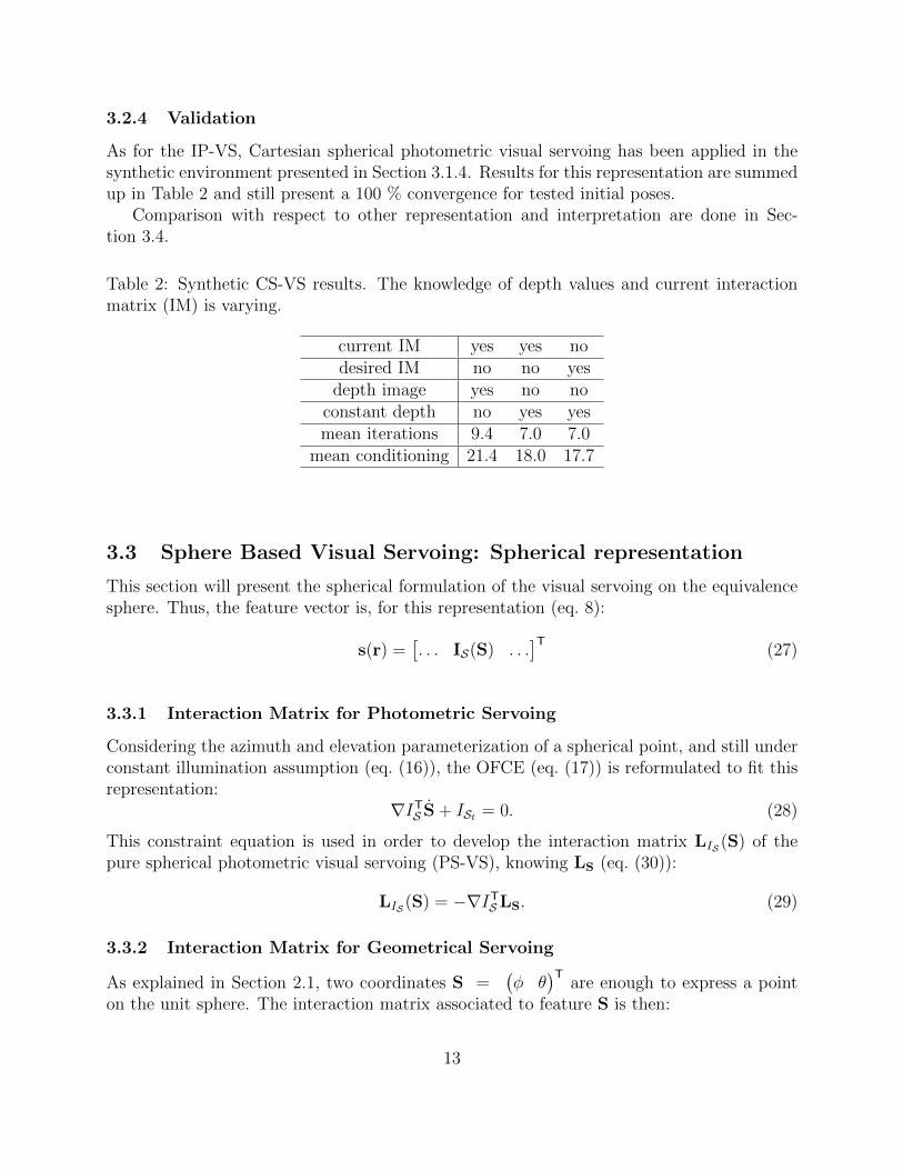
As for the IP-VS, Cartesian spherical photometric visual servoing has been applied in thesynthetic environment presented in Section 3.1.4. Results for this representation are summedup in Table 2 and still present a 100 % convergence for tested initial poses.

Comparison with respect to other representation and interpretation are done in Sec-tion 3.4.

Table 2: Synthetic CS-VS results. The knowledge of depth values and current interactionmatrix (IM) is varying.

current IM yes yes nodesired IM no no yes

depth image yes no noconstant depth no yes yesmean iterations 9.4 7.0 7.0

mean conditioning 21.4 18.0 17.7

3.3 Sphere Based Visual Servoing: Spherical representation

This section will present the spherical formulation of the visual servoing on the equivalencesphere. Thus, the feature vector is, for this representation (eq. 8):

s(r) =[. . . IS(S) . . .

]T(27)

3.3.1 Interaction Matrix for Photometric Servoing

Considering the azimuth and elevation parameterization of a spherical point, and still underconstant illumination assumption (eq. (16)), the OFCE (eq. (17)) is reformulated to fit thisrepresentation:

∇ITS S + ISt = 0. (28)

This constraint equation is used in order to develop the interaction matrix LIS (S) of thepure spherical photometric visual servoing (PS-VS), knowing LS (eq. (30)):

LIS (S) = −∇ITSLS. (29)

3.3.2 Interaction Matrix for Geometrical Servoing

As explained in Section 2.1, two coordinates S =(φ θ

)Tare enough to express a point

on the unit sphere. The interaction matrix associated to feature S is then:

13

(a) image plane (b) cartesian spherical

(c) pure spherical

Figure 6: Exponential curve fitting on residual decrease. Blue curves are mean residualsover (normalized) time and black curves, the exponential fitting.

LS =∂S

∂X

∂X

∂r=

(− cθcφ

ρ− sθcφ

ρsφρ

sθ −cθ 0sθρsφ

− cθρsφ

0 cθcφsφ

sθcφsφ

−1

)(30)

with cθ = cos θ, cφ = cosφ, sθ = sin θ, sφ = sinφ. This pure spherical formulation of visualservoing is minimal but has a singularity when sin φ = 0, i.e. when x = y = 0 inthe normalized image plane (principal point). Furthermore, this representation leads to aninteraction matrix more non linear than in the Cartesian spherical case, due to trigonometricfunctions.

3.3.3 Gradient Computation

To approximate the image gradient ∇IS on the sphere, we estimate ∂IS∂θ

and ∂IS∂φ

by usinga finite difference. We need to chose values for ∆θ, ∆φ and to interpolate the value of theintensity at this point. The reader can see [17] and our previous paper [7] to see the detailsof the direct pure spherical image gradient computation.

14

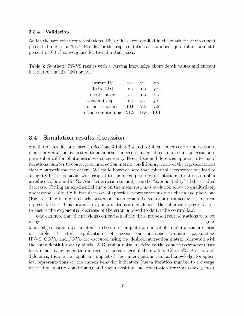
3.3.4 Validation

As for the two other representations, PS-VS has been applied in the synthetic environmentpresented in Section 3.1.4. Results for this representation are summed up in table 4 and stillpresent a 100 % convergence for tested initial poses.

Table 3: Synthetic PS-VS results with a varying knowledge about depth values and currentinteraction matrix (IM) or not.

current IM yes yes nodesired IM no no yes

depth image yes no noconstant depth no yes yesmean iterations 10.0 7.2 7.3

mean conditioning 21.3 18.0 19.1

3.4 Simulation results discussion

Simulation results presented in Sections 3.1.4, 3.2.4 and 3.3.4 can be crossed to understandif a representation is better than another between image plane, cartesian spherical andpure spherical for photometric visual servoing. Even if some differences appear in terms ofiterations number to converge or interaction matrix conditioning, none of the representationsclearly outperforms the others. We could however note that spherical representations lead toa slightly better behavior with respect to the image plane representation: iterations numberis reduced of around 23 %. Another criterion to analyze is the “exponentiality” of the residualdecrease. Fitting an exponential curve on the mean residuals evolution allow to qualitativelyunderstand a slightly better decrease of spherical representations over the image plane one(Fig. 6). The fitting is clearly better on mean residuals evolution obtained with sphericalrepresentations. This means less approximations are made with the spherical representationsto ensure the exponential decrease of the error imposed to derive the control law.

One can note that the previous comparison of the three proposed representations were ledusing goodknowledge of camera parameters. To be more complete, a final set of simulations is presentedin table 4 after application of noise on intrinsic camera parameters.IP-VS, CS-VS and PS-VS are executed using the desired interaction matrix computed withthe same depth for every pixels. A Gaussian noise is added to the camera parameters usedfor virtual image generation in terms of percentages of their value: 1% to 5%. As the table4 denotes, there is no significant impact of the camera parameters bad knowledge for spher-ical representations on the chosen behavior indicators (mean iteration number to converge,interaction matrix conditioning and mean position and orientation error at convergence).

15

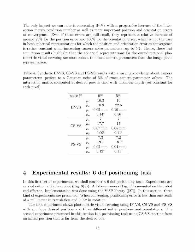
The only impact we can note is concerning IP-VS with a progressive increase of the inter-action matrix condition number as well as more important position and orientation errorsat convergence. Even if these errors are still small, they represent a relative increase ofaround 20% for the position error and 400% for the orientation error, which is not the casein both spherical representations for which the position and orientation error at convergenceis rather constant when increasing camera noise parameters, up to 5%. Hence, these lastsimulation results highlight that the spherical representations for the omnidirectional pho-tometric visual servoing are more robust to noised camera parameters than the image planerepresentation.

Table 4: Synthetic IP-VS, CS-VS and PS-VS results with a varying knowledge about cameraparameters: perfect to a Gaussian noise of 5% of exact camera parameter values. Theinteraction matrix computed at desired pose is used with unknown depth (set constant foreach pixel).

noise % 0% 5%

IP-VS

µi 10.3 10µc 18.8 22.6µt 0.05 mm 0.19 mmµo 0.14o 0.56o

CS-VS

µi 7 7µc 17.7 17µt 0.07 mm 0.05 mmµo 0.09o 0.11o

PS-VS

µi 7.3 7.2µc 19.1 18.7µt 0.05 mm 0.04 mmµo 0.12o 0.11o

4 Experimental results: 6 dof positioning task

In this first set of experiments, we shall consider a 6 dof positioning task. Experiments arecarried out on a Gantry robot (Fig. 8(b)). A fisheye camera (Fig. 1) is mounted on the robotend-effector. Implementation was done using the ViSP library ([27]). In this section, threekind of experiments are presented. When converging, positioning error is less than one tenthof a millimeter in translation and 0.02o in rotation.

The first experiment shows photometric visual servoing using IP-VS, CS-VS and PS-VSwith a unique desired position and three different initial positions and orientations. Thesecond experiment presented in this section is a positioning task using CS-VS starting froman initial position that is far from the desired one.

16

For all experiments, the interaction matrix is computed only at the desired position.Furthermore, the depth Z is an unknown parameter and is supposed constant for all pixels,along the motion of the camera. The achievement of experiments shows the method is robustto a coarse estimation of Z.

Experiments were led using a Sony Vaio laptop with an Intel Centrino 1.2 GHz micro-processor, 2 GB RAM and running Windows XP, for image acquisition and computation ofcontrol vectors. Without any particular code optimization, the loop can been closed at 20 Hzfor images of 640x480 pixels, which is close to standard camera acquisition framerate. Betterimplementation and the use of the GPU could easily make the processing faster. Since thereare no geometrical features to extract, track and match, the image processing step is quitestraightforward (gradient computation) and is timeless.

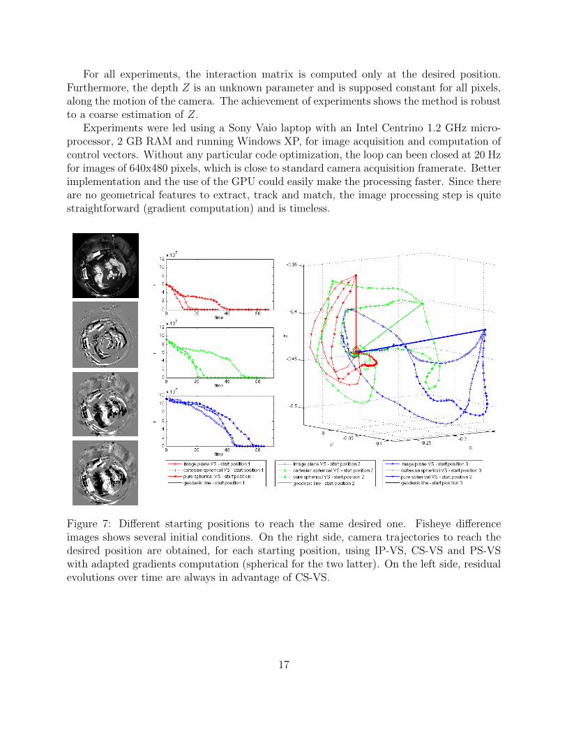
Figure 7: Different starting positions to reach the same desired one. Fisheye differenceimages shows several initial conditions. On the right side, camera trajectories to reach thedesired position are obtained, for each starting position, using IP-VS, CS-VS and PS-VSwith adapted gradients computation (spherical for the two latter). On the left side, residualevolutions over time are always in advantage of CS-VS.

17

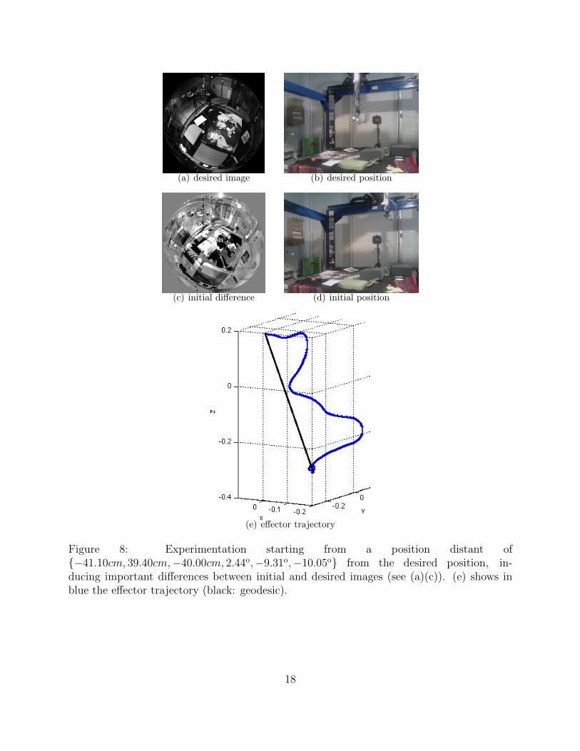
(a) desired image (b) desired position

(c) initial difference (d) initial position

(e) effector trajectory

Figure 8: Experimentation starting from a position distant of{−41.10cm, 39.40cm,−40.00cm, 2.44o,−9.31o,−10.05o} from the desired position, in-ducing important differences between initial and desired images (see (a)(c)). (e) shows inblue the effector trajectory (black: geodesic).

18

4.1 Behavior evaluation for different initial poses

IP-VS, CS-VS and PS-VS are compared using standard image gradients computation forIP-VS and Cartesian spherical, resp. pure spherical gradients for CS-VS, resp. PS-VS.These gradients computations are theoretically and practically more valid than other com-putations ([7]). Results are presented in Figure 7.

Omnidirectional photometric visual servoing is done from three different initial positionsto a unique desired position. Errors {∆X ,∆Y ,∆Z ,∆RX

,∆RY,∆RZ

} between desired and ini-tial positions are respectively {0cm, 0cm,−8.2cm, 0o, 0o, 0o}, {−8.7cm,−0.1cm,−4.5cm,−2.4o, 11.4o, 8.0o} and {−15.9cm,−1.6cm,−1.3cm, 2.5o, 14.6o, 7.4o}. The latter experiment is the hardest situation, with a transla-tion along the X axis and a rotation around the Y axis, leading to projective ambiguities.Hence, the shape of the cost function leads to less straight motions. Figure 7 shows initialimages of differences and the third initial position produces the most important difference.Indeed, trajectories of IP-VS, CS-VS and PS-CS are the most different for the latter ex-periment. Residuals evolution over time (Fig. 7, left), always show that CS-VS convergesfaster.

4.2 Large motion

This experiment aims to show this technique can be used for relatively large motions. CS-VSwas the only formulation allowing to converge. A possible interpretation of this result is thatthe translation in camera frame is mostly along optical axis and this representation has a Zcomponent in equations, particularly in the spherical image gradient. The initial camera posi-tion is such that the initial positioning error is {−41.1cm, 39.4cm,−40.0cm, 2.4o,−9.3o,−10.1o}.Despite important position and coupled orientations differences, which is highlighted by fig-ure 8(c), photometric visual servoing succeeds. Figure 8(e) shows resulting camera trajectoryin robot frame.

4.3 Six dof experimental results discussion

The precision at convergence is very similar to the one reached in the perspective case forwhich a comparison with a basic visual feature control law has been done. As reportedin ([12]), SURF keypoints along with a classical or statistically robust control law havebeen considered. As expected, in that case, if detection and matching succeeds with nolost features, the convergence area is larger than in the photometric case. It remains thatkeypoint matching is still a difficult issue (especially in the case of catadioptric sensor) andthat an incorrect matching could jeopardize the achievement of the task.

Furthermore, higher precision was obtained with the photometric feature rather thanwith the points, mainly for two reasons. Firstly, even when successful, geometric featurematching always features some uncertainty leading to imprecision in the repositioning task.Secondly, the photometric servoing control law is computed with dense information ratherthan sparse, leading to a higher precision thanks to feature redundancy. Let us note that, in

19

the perspective case, the final positioning precision is, in translation, ten times more precisewith the photometric feature than with SURF points.

Since similar repositioning precisions, using a photometric scheme, have been obtainedwith perspective and catadioptric cameras (on the same robot), similar conclusions in bothcases can then be extrapolated but have not been verified due to the lack of an efficientkeypoint matching algorithm on omnidirectional images.

5 Application to mobile robot navigation

This section aims to define and evaluate a path following task with a mobile robot using aset of images as waypoints. Photometric visual servoing is applied on each image, one byone, in order to follow the path. We will first tackle the positioning of a mobile robot usingone desired image and modeling the robot motion in a simple scheme.

5.1 Formulation

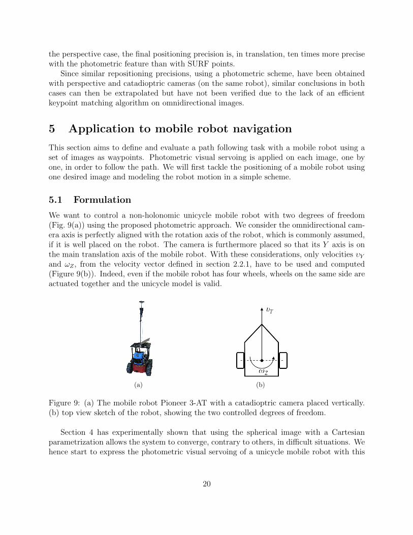
We want to control a non-holonomic unicycle mobile robot with two degrees of freedom(Fig. 9(a)) using the proposed photometric approach. We consider the omnidirectional cam-era axis is perfectly aligned with the rotation axis of the robot, which is commonly assumed,if it is well placed on the robot. The camera is furthermore placed so that its Y axis is onthe main translation axis of the mobile robot. With these considerations, only velocities υYand ωZ , from the velocity vector defined in section 2.2.1, have to be used and computed(Figure 9(b)). Indeed, even if the mobile robot has four wheels, wheels on the same side areactuated together and the unicycle model is valid.

(a) (b)

Figure 9: (a) The mobile robot Pioneer 3-AT with a catadioptric camera placed vertically.(b) top view sketch of the robot, showing the two controlled degrees of freedom.

Section 4 has experimentally shown that using the spherical image with a Cartesianparametrization allows the system to converge, contrary to others, in difficult situations. Wehence start to express the photometric visual servoing of a unicycle mobile robot with this

20

formulation. The interaction matrix linked to the intensity of a spherical point w.r.t. themobile robot camera motion is LIS(XS) = −∇ITSLXS ,with (eq. (24)):

LXS =

XSYSρ

YSY 2S−1ρ

−XSYSZSρ

0

. (31)

However, we saw, despite the large motion, PS-VS and CS-VS are rather close in termsof performance. So we define the interaction matrix between the motion of a point and thecamera velocity for the pure spherical representation:

LS =

(− sin θ cosφ

ρ0

− cos θρ sinφ

−1

). (32)

This interaction matrix, deduced from equation (30), shows a decoupling property betweenthe control of the translational and rotational velocities ([34]). This matrix substitutes thegeometrical interaction matrix in equation (29) to get the interaction matrix linked to theintensity of a spherical point w.r.t. the camera motion.

5.2 Experiments

Pure spherical and Cartesian representations are compared. The former clearly shows theo-retical advantages and the latter is practically more efficient in a six d.o.f. control, when alarge motion is considered.

As in the six d.o.f. visual servoing, the desired omnidirectional image as a whole is thetarget to be reached, wherever are a particular object within the scene or within the image.Considering the mobile robot, the robot seems to move toward a target but this is inherentto the non-holonomic constraints of the considered system. Indeed, if a holonomic systemwas considered any kind of motion in any direction could have been considered as it was thecase with the six d.o.f gantry robot.

5.2.1 Validation and evaluation experiments

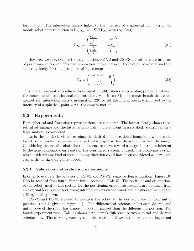
In order to evaluate the behavior of CS-VS and PS-VS, a unique desired position (Figure 10)is to be reached from four different initial positions (Tab. 5). The positions and orientationsof the robot, used in this section for the positioning error measurement, are obtained froman external localization tool, using infrared makers on the robot and a camera placed at theceiling, looking down.

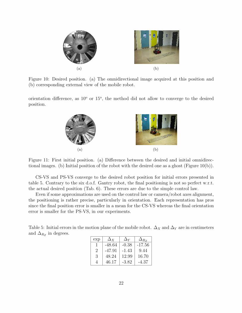
CS-VS and PS-VS succeed to position the robot at the desired place for four initialpositions (one is given in figure 11). The difference of orientation between desired andinitial pose of the robot has a more important impact than the difference in position. Thefourth experimentation (Tab. 5) shows here a weak difference between initial and desiredorientations. The servoing converges in this case but if we introduce a more important

21

(a) (b)

Figure 10: Desired position. (a) The omnidirectional image acquired at this position and(b) corresponding external view of the mobile robot.

orientation difference, as 10o or 15o, the method did not allow to converge to the desiredposition.

(a) (b)

Figure 11: First initial position. (a) Difference between the desired and initial omnidirec-tional images. (b) Initial position of the robot with the desired one as a ghost (Figure 10(b)).

CS-VS and PS-VS converge to the desired robot position for initial errors presented intable 5. Contrary to the six d.o.f. Gantry robot, the final positioning is not so perfect w.r.t.the actual desired position (Tab. 6). These errors are due to the simple control law.

Even if some approximations are used on the control law or camera/robot axes alignment,the positioning is rather precise, particularly in orientation. Each representation has prossince the final position error is smaller in a mean for the CS-VS whereas the final orientationerror is smaller for the PS-VS, in our experiments.

Table 5: Initial errors in the motion plane of the mobile robot. ∆X and ∆Y are in centimetersand ∆RZ

in degrees.exp ∆X ∆Y ∆RZ

1 -48.64 -0.38 -17.562 -47.91 -1.43 9.443 48.24 12.99 16.704 46.17 -3.82 -4.37

22

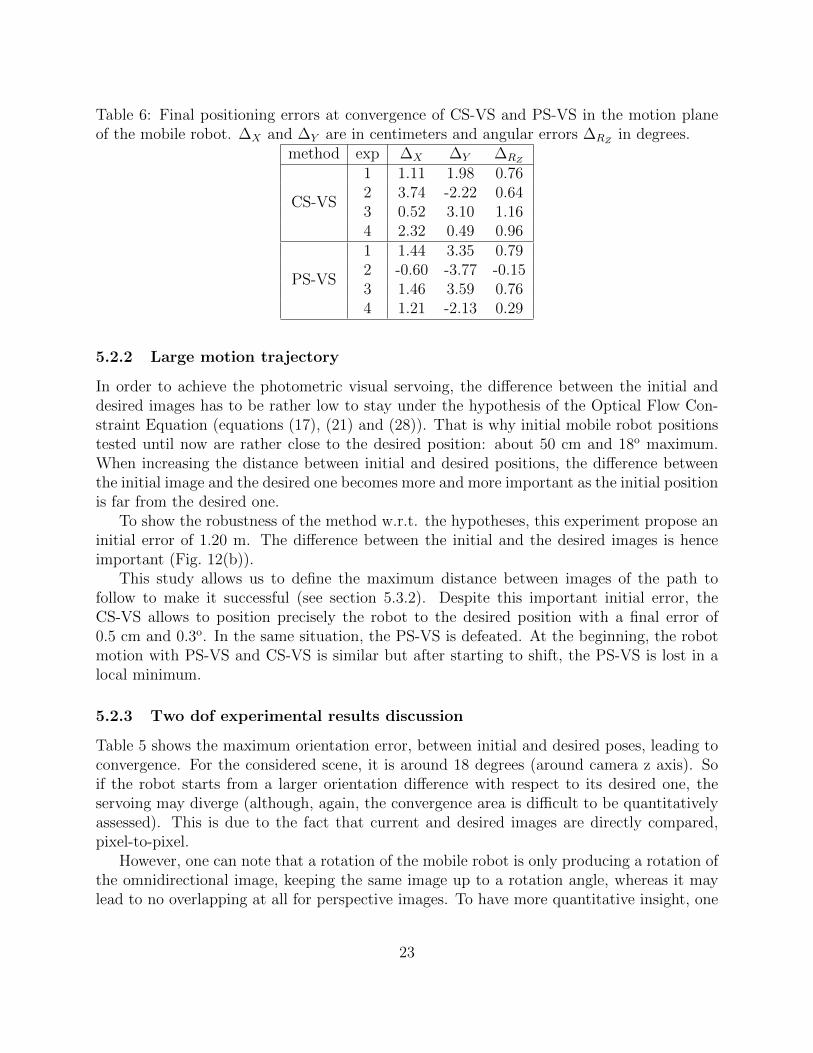
Table 6: Final positioning errors at convergence of CS-VS and PS-VS in the motion planeof the mobile robot. ∆X and ∆Y are in centimeters and angular errors ∆RZ

in degrees.method exp ∆X ∆Y ∆RZ

CS-VS

1 1.11 1.98 0.762 3.74 -2.22 0.643 0.52 3.10 1.164 2.32 0.49 0.96

PS-VS

1 1.44 3.35 0.792 -0.60 -3.77 -0.153 1.46 3.59 0.764 1.21 -2.13 0.29

5.2.2 Large motion trajectory

In order to achieve the photometric visual servoing, the difference between the initial anddesired images has to be rather low to stay under the hypothesis of the Optical Flow Con-straint Equation (equations (17), (21) and (28)). That is why initial mobile robot positionstested until now are rather close to the desired position: about 50 cm and 18o maximum.When increasing the distance between initial and desired positions, the difference betweenthe initial image and the desired one becomes more and more important as the initial positionis far from the desired one.

To show the robustness of the method w.r.t. the hypotheses, this experiment propose aninitial error of 1.20 m. The difference between the initial and the desired images is henceimportant (Fig. 12(b)).

This study allows us to define the maximum distance between images of the path tofollow to make it successful (see section 5.3.2). Despite this important initial error, theCS-VS allows to position precisely the robot to the desired position with a final error of0.5 cm and 0.3o. In the same situation, the PS-VS is defeated. At the beginning, the robotmotion with PS-VS and CS-VS is similar but after starting to shift, the PS-VS is lost in alocal minimum.

5.2.3 Two dof experimental results discussion

Table 5 shows the maximum orientation error, between initial and desired poses, leading toconvergence. For the considered scene, it is around 18 degrees (around camera z axis). Soif the robot starts from a larger orientation difference with respect to its desired one, theservoing may diverge (although, again, the convergence area is difficult to be quantitativelyassessed). This is due to the fact that current and desired images are directly compared,pixel-to-pixel.

However, one can note that a rotation of the mobile robot is only producing a rotation ofthe omnidirectional image, keeping the same image up to a rotation angle, whereas it maylead to no overlapping at all for perspective images. To have more quantitative insight, one

23

(a) (b)

(c)

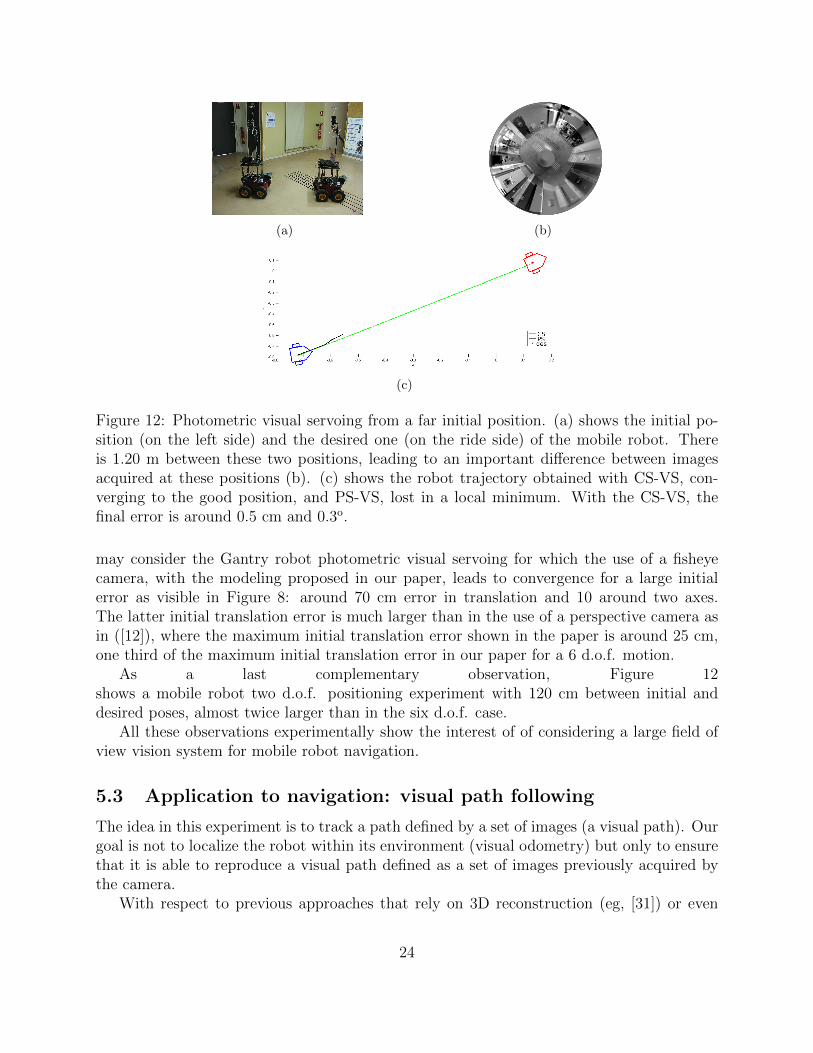
Figure 12: Photometric visual servoing from a far initial position. (a) shows the initial po-sition (on the left side) and the desired one (on the ride side) of the mobile robot. Thereis 1.20 m between these two positions, leading to an important difference between imagesacquired at these positions (b). (c) shows the robot trajectory obtained with CS-VS, con-verging to the good position, and PS-VS, lost in a local minimum. With the CS-VS, thefinal error is around 0.5 cm and 0.3o.

may consider the Gantry robot photometric visual servoing for which the use of a fisheyecamera, with the modeling proposed in our paper, leads to convergence for a large initialerror as visible in Figure 8: around 70 cm error in translation and 10 around two axes.The latter initial translation error is much larger than in the use of a perspective camera asin ([12]), where the maximum initial translation error shown in the paper is around 25 cm,one third of the maximum initial translation error in our paper for a 6 d.o.f. motion.

As a last complementary observation, Figure 12shows a mobile robot two d.o.f. positioning experiment with 120 cm between initial anddesired poses, almost twice larger than in the six d.o.f. case.

All these observations experimentally show the interest of of considering a large field ofview vision system for mobile robot navigation.

5.3 Application to navigation: visual path following

The idea in this experiment is to track a path defined by a set of images (a visual path). Ourgoal is not to localize the robot within its environment (visual odometry) but only to ensurethat it is able to reproduce a visual path defined as a set of images previously acquired bythe camera.

With respect to previous approaches that rely on 3D reconstruction (eg, [31]) or even

24

on appearance-based approaches ([32]), the learning step of the approach is simple. It doesnot require any feature extraction nor scene reconstruction: no image processing is done,only raw images are stored. The robot is driven manually along a desired path. While therobot is moving, the images acquired by the camera are stored chronologically thus defininga trajectory in the image space. Let us call I∗0 , . . . , I

∗N the key images that define this visual

path.The vehicle is initially positioned close to the initial position of the learned visual path

(defined by the image I∗0 ). The navigation is performed using a visual servoing task. In[31, 14, 32, 10] the considered control schemes are either pose-based control law or considerclassical visual servoing process based on the use of visual features extracted from the currentand key images (I and I∗k).

In this work the approach proposed in the previous section is used to navigate from awaypoint (key-image) to another.

Considering reasonable mean distances and orientation differences between waypoints, wepropose to apply the photometric visual servoing for the visual path following. A difficultyis to decide if a waypoint is reached to try to reach the next one. It is then necessary toknow when the current and desired images are the most similar. The ZNCC: Zero-meanNormalized Cross Correlation ([18]) is a good criterion for this issue. The SSD, i.e thecost function of the control law, has the drawback, in the navigation application, to beshifted when an illumination changing appears. This is not a problem for photometric visualservoing since even if the minimal value is not always the same, the corresponding optimalposition is the same. So, a fixed threshold on the SSD measure to know if the desired imageis reached would become wrong since the scene illumination can change. The ZNCC has, onthe contrary, the same value even if the global illumination changes. So, if the ZNCC betweenthe current and the desired image is greater than an experimentally chosen threshold (0.7 inexperimentations) and corresponding to a quasi perfect alignment between two images, theservoing is considered ended for the desired image associated to the waypoint. The robotlooks then for the next waypoint.

5.3.1 Visual path following

In this context, we considered that the translation velocity is a constant, leading to a one dofcontrol problem, i.e. the rotation velocity. Thus, from the interaction matrix of a Cartesianpoint of a spherical image for a unicycle mobile robot (eq. (31)), we directly obtain the oneconcerning the rotation dof only:

LXS =

YS−XS

0

. (33)

The latter interaction matrix does not depend anymore on the point deepness ρ which has tobe noted (it was approximated before). The composition of this Jacobian with the Cartesianspherical gradients leads to the interaction matrix linked to the intensity of a spherical pointw.r.t. the mobile camera motion.

25

Dealing with the pure spherical formulation, the interaction matrix for a point for thevisual path following is:

LS =

(0

−1

), (34)

which does not depend on the 3D point deepness too. The latter interaction matrix isfurthermore constant, anywhere on the sphere. The photometric interaction matrix forthe pure spherical representation is then obtained from the composition between the purespherical gradients and the Jacobian of equation (34).

The advantage to consider the translation velocity as a constant is to lose the deepnessparameter ρ of the interaction matrix. It only depends now on information directly obtainedfrom the image: the backprojection of a pixel coordinates on the sphere and the sphericalgradient.

5.3.2 Experimental results

Validation on a short curved path The visual memory is composed by an image se-quence acquired in a learning stage in which the robot is manually driven. Omnidirectionalimages are acquired with 30 cm or 10o between them, using odometers of the robot. These30 cm and 10o distances are empirically deduced from table 5. The experimentation isled over a curved trajectory of 3.5 m with 20 reference images. The interaction matricescomputation is then done offline before starting the path following.

The path following, done by successive photometric visual servoing on each referenceimage, leads to slightly different trajectories if the spherical representation is used or theCartesian one (Fig. 13). Positions and orientations of the robot are obtained with theexternal localization tool previously mentioned.

Application to a round trip After the validation of the visual path following in a smallarea but for a highly curved path, we changed the environment of the robot and also usedanother omnidirectional camera which is more compact. In this experiment, key images arestill acquired every 30 cm or 10o but along a path of 20 m. The goal of the robot is to go tothe end of its visual path and then to come back at its original position following the inversevisual path. So a total path length of 40 m has to be traveled. In addition to this morechallenging path length, the environment is now rather textureless and natural light troughwindows at the end of the path is varying. People are also walking in the environment causingits partial occlusion. Despite these much more challenging conditions than in the previousexperiment, the omnidirectional photometric visual path following succeeds with a correctprecision in execution of the path as figure 14 qualitatively shows. It also demonstrates thata precise localization of the camera/robot along the path is not necessary to precisely achievea navigation task.

26

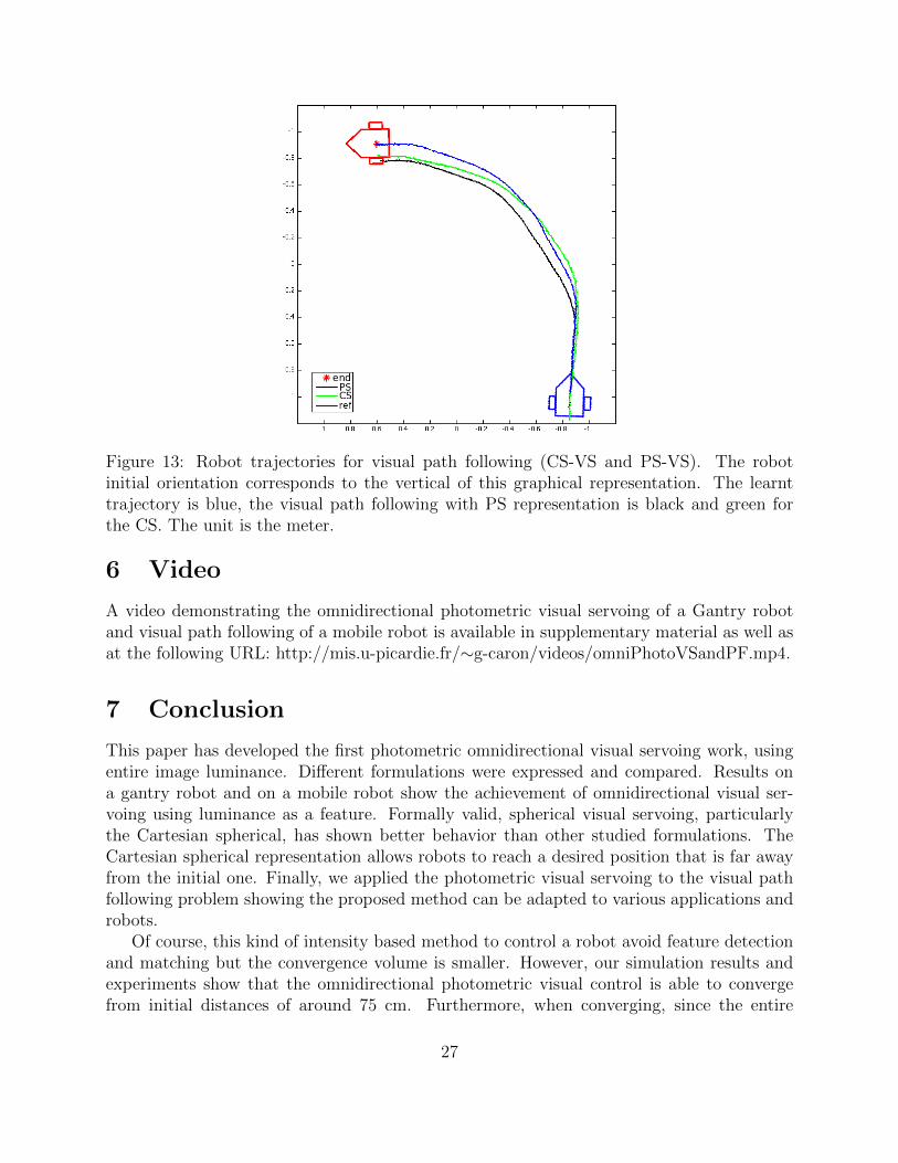
Figure 13: Robot trajectories for visual path following (CS-VS and PS-VS). The robotinitial orientation corresponds to the vertical of this graphical representation. The learnttrajectory is blue, the visual path following with PS representation is black and green forthe CS. The unit is the meter.

6 Video

A video demonstrating the omnidirectional photometric visual servoing of a Gantry robotand visual path following of a mobile robot is available in supplementary material as well asat the following URL: http://mis.u-picardie.fr/∼g-caron/videos/omniPhotoVSandPF.mp4.

7 Conclusion

This paper has developed the first photometric omnidirectional visual servoing work, usingentire image luminance. Different formulations were expressed and compared. Results ona gantry robot and on a mobile robot show the achievement of omnidirectional visual ser-voing using luminance as a feature. Formally valid, spherical visual servoing, particularlythe Cartesian spherical, has shown better behavior than other studied formulations. TheCartesian spherical representation allows robots to reach a desired position that is far awayfrom the initial one. Finally, we applied the photometric visual servoing to the visual pathfollowing problem showing the proposed method can be adapted to various applications androbots.

Of course, this kind of intensity based method to control a robot avoid feature detectionand matching but the convergence volume is smaller. However, our simulation results andexperiments show that the omnidirectional photometric visual control is able to convergefrom initial distances of around 75 cm. Furthermore, when converging, since the entire

27

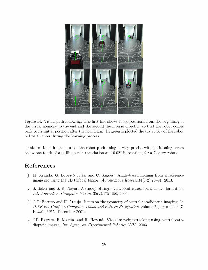
Figure 14: Visual path following. The first line shows robot positions from the beginning ofthe visual memory to the end and the second the inverse direction so that the robot comesback to its initial position after the round trip. In green is plotted the trajectory of the robotred part center during the learning process.

omnidirectional image is used, the robot positioning is very precise with positioning errorsbelow one tenth of a millimeter in translation and 0.02o in rotation, for a Gantry robot.

References

[1] M. Aranda, G. Lopez-Nicolas, and C. Sagues. Angle-based homing from a referenceimage set using the 1D trifocal tensor. Autonomous Robots, 34(1-2):73–91, 2013.

[2] S. Baker and S. K. Nayar. A theory of single-viewpoint catadioptric image formation.Int. Journal on Computer Vision, 35(2):175–196, 1999.

[3] J. P. Barreto and H. Araujo. Issues on the geometry of central catadioptric imaging. InIEEE Int. Conf. on Computer Vision and Pattern Recognition, volume 2, pages 422–427,Hawaii, USA, December 2001.

[4] J.P. Barreto, F. Martin, and R. Horaud. Visual servoing/tracking using central cata-dioptric images. Int. Symp. on Experimental Robotics VIII., 2003.

28

[5] H. Becerra, G. Lopez-Nicolas, and C. Sagues. Omnidirectional visual control of mobilerobots based on the 1D trifocal tensor. Robotics and Autonomous Systems, 58(6):796–808, 2010.

[6] S. Benhimane and E. Malis. Homography-based 2d visual tracking and servoing. Int.Journal of Robotics Research, 26(7):661–676, 2007.

[7] G. Caron, E. Marchand, and E. Mouaddib. Omnidirectional photometric visual servoing.In IEEE/RSJ Int. Conf. on Intelligent Robots and Systems, pages 6202–6207, Taipei,Taiwan, October 2010.

[8] F. Chaumette. Image moments: a general and useful set of features for visual servoing.IEEE Trans. on Robotics, 20(4):713–723, August 2004.

[9] F. Chaumette and S. Hutchinson. Visual servo control, Part I: Basic approaches. IEEERobotics and Automation Magazine, 13(4):82–90, December 2006.

[10] Z. Chen and S.T. Birchfield. Qualitative vision-based path following. IEEE Transactionson Robotics, 25(3):749–754, 2009.

[11] G. Chesi and K Hashimoto, editors. Visual servoing via advanced numerical methods.LNCIS 401. Springer, 2010.

[12] C. Collewet and E. Marchand. Photometric visual servoing. IEEE Trans. on Robotics,27(4):828–834, 2011.

[13] J. Courbon, Y. Mezouar, L. Eck, and P. Martinet. A generic fisheye camera model forrobotic applications. In IEEE/RSJ Int. Conf. on Intelligent Robots and System, pages1683–1688, San Diego, USA, October 2007.

[14] J. Courbon, Y. Mezouar, and P. Martinet. Autonomous navigation of vehicles from avisual memory using a generic camera model. IEEE Trans. on Intelligent TransportationSystems, 10(3):392–402, 2009.

[15] A. Dame and E. Marchand. Mutual information-based visual servoing. IEEE Trans. onRobotics, 27(5):958–969, 2011.

[16] K. Deguchi. A direct interpretation of dynamic images with camera and object motionsfor vision guided robot control. Int. Journal on Computer Vision, 37(1):7–20, 2000.

[17] C. Demonceaux and P. Vasseur. Omnidirectional image processing using geodesic met-ric. In Int. Conf. on Image Processing, pages 221–224, Cairo, Egypt, November 2009.

[18] L. Di Stephano, S. Mattoccia, and F. Tombari. ZNCC-based template matching usingbounded partial correlation. Pattern Recognition Letters, 26:2129–2134, 2005.

[19] B. Espiau, F. Chaumette, and P. Rives. A new approach to visual servoing in robotics.IEEE Trans. on Robotics and Automation, 8(3):313–326, June 1992.

29

[20] T. Hamel and R. Mahony. Visual servoing of an under-actuated dynamic rigid-body sys-tem: An image-based approach. IEEE Trans. on Robotics and Automation, 18(2):187–198, 2002.

[21] B. Horn and Schunck. Determining optical flow. Artificial Intelligence, 17:185–203,1981.

[22] S. Hutchinson, G. Hager, and P. Corke. A tutorial on visual servo control. IEEE Trans.on Robotics and Automation, 12:651–670, 1996.

[23] V. Kallem, M. Dewan, J.P. Swensen, G.D. Hager, and N.J. Cowan. Kernel-based visualservoing. In IEEE/RSJ Int. Conf. on Intelligent Robots and System, pages 1975–1980,San Diego, USA, October 2007.

[24] P. Lebraly, C. Deymier, O. Ait-Aider, E. Royer, and M. Dhome. Flexible extrinsiccalibration of non-overlapping cameras using a planar mirror: Application to vision-based robotics. In IEEE/RSJ Int. Conf. on Intelligent Robots and System, pages 5640–5647, Taipei, Taiwan, October 2010.

[25] E. Malis. Improving vision-based control using efficient second-order minimization tech-niques. In IEEE Int. Conf. on Robotics and Automation, volume 2, pages 1843–1848,New Orleans, April 2004.

[26] E. Marchand and F. Chaumette. Feature tracking for visual servoing purposes. Roboticsand Autonomous Systems, 52(1):53–70, July 2005.

[27] E. Marchand, F. Spindler, and F. Chaumette. Visp for visual servoing: a generic soft-ware platform with a wide class of robot control skills. IEEE Robotics and AutomationMagazine, 12(4):40–52, December 2005.

[28] G. Mariottini and D. Prattichizzo. Image-based visual servoing with central catadioptriccameras. Int. J. of Robotics Research, 27(1):41–56, 2008.

[29] M. Meilland, A. I. Comport, and P. Rives. Dense visual mapping of large scale envi-ronments for real-time localization. In IEEE/RSJ Int. Conf. on Intelligent Robots andSystem, pages 4242 –4248, San Francisco, CA, sept. 2011.

[30] S.K. Nayar, S.A. Nene, and H. Murase. Subspace methods for robot vision. IEEETrans. on Robotics and Automation, 12(5):750–758, October 1996.

[31] E. Royer, M. Lhuillier, M. Dhome, and J.M. Lavest. Monocular vision for mobile robotlocalization and autonomous navigation. Int. Journal of Computer Vision, 74(3):237–260, 2007.

[32] S. Segvic, A. Remazeilles, A. Diosi, and F. Chaumette. A mapping and localizationframework for scalable appearance-based navigation. Computer Vision and Image Un-derstanding, 113(2):172–187, February 2009.

30

[33] O. Tahri, Y. Mezouar, F. Chaumette, and P. Corke. Decoupled image-based visualservoing for cameras obeying the unified projection model. IEEE Trans. on Robotics,26(4):684–697, 2010.

[34] R. Tatsambon Fomena, H. Yoon, A. Cherubini, F. Chaumette, and S. Hutchinson.Coarsely calibrated visual servoing of a mobile robot using a catadioptric vision system.In IEEE Int. Conf. on Intelligent Robots and Systems, pages 5432–5437, St Louis, USA,October 2009.

[35] X. Ying and Z. Hu. Can we consider central catadioptric cameras and fisheye cameraswithin a unified imaging model. In Eur. Conf. on Comp. Vision, pages 442–455, Prague,Czech Republic, May 2004.

31