Modelling and Nonlinear Analysis of Aircraft Ground Manoeuvresec1099/ECoetzee_PhD_Thesis.pdf ·...
123
Modelling and Nonlinear Analysis of Aircraft Ground Manoeuvres Etienne Coetzee Department of Engineering Mathematics University of Bristol A dissertation submitted to the University of Bristol in accordance with the requirements of the degree of Doctor of Philosophy in the Faculty of Engineering. February 2011
Transcript of Modelling and Nonlinear Analysis of Aircraft Ground Manoeuvresec1099/ECoetzee_PhD_Thesis.pdf ·...
Modelling and Nonlinear Analysis of AircraftGround Manoeuvres
Etienne Coetzee
Department of Engineering Mathematics
University of Bristol
A dissertation submitted to the University of Bristol in
accordance with the requirements of the degree of
Doctor of Philosophy in the Faculty of Engineering.
February 2011

Abstract
Recent studies in the USA and Europe show that passenger numbers are doubling every 15years, with a consequent increase in traffic and a demand for new airframes. More efficient sur-face movements will alleviate congestion due to this growth. An understanding of the grounddynamics of different sized aircraft is therefore essential. The objective of this thesis is to clas-sify the ground dynamics of different sized aircraft across the entire operational and designenvelope. The nonlinear nature of the problem generally adds to the complexity of such dy-namics, where small perturbations in velocity, steering angle or brake application may lead tosignificant differences in the performance that can be achieved. The use of industrially testedmodels of the A320 and A380 are an important aspect of this work. Good agreement is shownbetween simulation results and flight test data, underpinning the validity of the models. Thesemodels are constructed in the MSC.Adams and SimMechanics software environments, whereall relevant information in terms of steering angles, clearance distances, and tyre forces areprovided. The computational challenges related to multibody simulations are highlighted, andconsequently alternative analysis methods are explored. The most widely employed analysismethods that can be used to study aircraft ground manoeuvres consist of geometric, kinematic,dynamic, and bifurcation methods. To allow for the nonlinear analysis of industrially-testedmodels in a user-friendly environment, AUTO has been integrated with Matlab in the form of aDynamical Systems Toolbox. The SimMechanics aircraft models are coupled to AUTO withinthis new toolbox, where AUTO has direct access to the states, even though the model equationsare a black-box to the user. This is an important capability that allows one to integrate exist-ing validated models with the bifurcation software, avoiding significant effort in redevelopingmodels for bifurcation analysis.
We show that widely used geometric methods for the calculation of turn widths are not applica-ble to large aircraft such as the A380, due to the asymmetric thrust and braking inputs that arerequired for the U-turn manoeuvre. Bifurcation and continuation methods, on the other hand,are shown to be effective for the analysis of this type of manoeuvre at a fraction of the costof simulations. The presence of a fold bifurcation provides new insight into the dynamics ofU-turn manoeuvres, which is not easily observed from simulation data. Kinematic equationsare used to analyse the stability of an aircraft that is being towed, where we conclude that jack-knifing can be avoided by maintaining a towing radius that is larger than the wheel base. Theyalso form the basis of the runway exit studies, from which empirical formulas are derived forsteering angle and clearance predictions. The results of the empirical method compare verywell with kinematic studies, as well as detailed dynamic model simulations, as is demonstratedwith a test case example of an A380 model. The empirical formulas can be used to great effectduring the early design phases of an aircraft programme for the prediction of steering anglesand clearance distances, when very little data is available. The greatest advantage of the pro-posed method is that any aircraft configuration or runway exit can be analysed. The steady-stateforce values that are provided from continuation methods can be used to evaluate the FAA 0.5ghigh-speed lateral ground loads regulation. A strong correlation exists between the results fromthe analysis and the measurements from an operational loads test campaign. We show that theA380 can only generate a load that is half the value stipulated by the regulation. This is due tothe nonlinear nature of the tyre properties and the overwhelming influence of the aerodynamicsat higher velocities. This analysis provides additional evidence that a lateral load factor of 0.5cannot be reached for such a large aircraft.

Acknowledgements
I would like to thank my supervisors, Prof. Bernd Krauskopf and Dr. Mark Lowenberg, for theircontinued support and encouragement. Without their guidance and expertise this PhD wouldnot have been possible. I would also like to thank my industrial supervisor at Airbus, SanjivSharma, who has supported all the nonlinear dynamics activities at Airbus since 2003. He hasbeen instrumental in advocating their use within an industrial context. I owe Airbus immensegratitude for allowing me to pursue this PhD, and I hope the results speak for themselves. I alsowould like to thank Bob Thompson at Airbus for his valuable inputs, especially with regardsto the explanation of some of the operational usage scenarios. Thanks also to James Rankinand Phani Thota who helped to lay the foundations for many of the projects that have followed.I would like to thank my family in South Africa and in the United Kingdom, who have beenright behind me every step of the way. Lastly, I would like to thank my lovely wife Sarah forher patience, and our eight week old daughter, Elana, for giving me some added incentive tocomplete this work before she was born.


“Science is built up with facts, as a house is with stones.But a collection of facts is no more a science than a heap of stones is a house.”
Henri Poincaré

Author’s Declaration
I declare that the work in this dissertation was carried out in accordance with the regulations ofthe University of Bristol. The work is original except where indicated by special reference inthe text and no part of the dissertation has been submitted for any other degree.
Any views expressed in the dissertation are those of the author and in no way represent thoseof the University of Bristol.
The dissertation has not been presented to any other University for examination either in theUnited Kingdom or overseas.
Signed:
Dated:

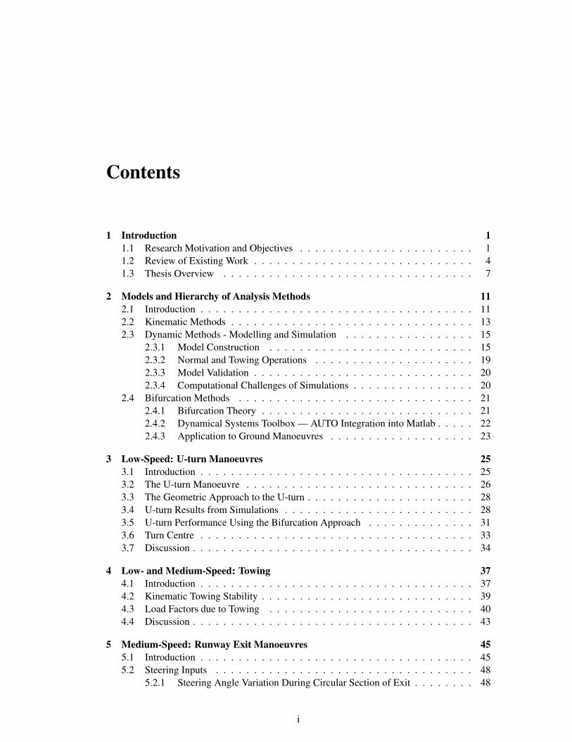
Contents
1 Introduction 11.1 Research Motivation and Objectives . . . . . . . . . . . . . . . . . . . . . . . 11.2 Review of Existing Work . . . . . . . . . . . . . . . . . . . . . . . . . . . . . 41.3 Thesis Overview . . . . . . . . . . . . . . . . . . . . . . . . . . . . . . . . . 7
2 Models and Hierarchy of Analysis Methods 112.1 Introduction . . . . . . . . . . . . . . . . . . . . . . . . . . . . . . . . . . . . 112.2 Kinematic Methods . . . . . . . . . . . . . . . . . . . . . . . . . . . . . . . . 132.3 Dynamic Methods - Modelling and Simulation . . . . . . . . . . . . . . . . . 15
2.3.1 Model Construction . . . . . . . . . . . . . . . . . . . . . . . . . . . 152.3.2 Normal and Towing Operations . . . . . . . . . . . . . . . . . . . . . 192.3.3 Model Validation . . . . . . . . . . . . . . . . . . . . . . . . . . . . . 202.3.4 Computational Challenges of Simulations . . . . . . . . . . . . . . . . 20
2.4 Bifurcation Methods . . . . . . . . . . . . . . . . . . . . . . . . . . . . . . . 212.4.1 Bifurcation Theory . . . . . . . . . . . . . . . . . . . . . . . . . . . . 212.4.2 Dynamical Systems Toolbox — AUTO Integration into Matlab . . . . . 222.4.3 Application to Ground Manoeuvres . . . . . . . . . . . . . . . . . . . 23
3 Low-Speed: U-turn Manoeuvres 253.1 Introduction . . . . . . . . . . . . . . . . . . . . . . . . . . . . . . . . . . . . 253.2 The U-turn Manoeuvre . . . . . . . . . . . . . . . . . . . . . . . . . . . . . . 263.3 The Geometric Approach to the U-turn . . . . . . . . . . . . . . . . . . . . . . 283.4 U-turn Results from Simulations . . . . . . . . . . . . . . . . . . . . . . . . . 283.5 U-turn Performance Using the Bifurcation Approach . . . . . . . . . . . . . . 313.6 Turn Centre . . . . . . . . . . . . . . . . . . . . . . . . . . . . . . . . . . . . 333.7 Discussion . . . . . . . . . . . . . . . . . . . . . . . . . . . . . . . . . . . . . 34
4 Low- and Medium-Speed: Towing 374.1 Introduction . . . . . . . . . . . . . . . . . . . . . . . . . . . . . . . . . . . . 374.2 Kinematic Towing Stability . . . . . . . . . . . . . . . . . . . . . . . . . . . . 394.3 Load Factors due to Towing . . . . . . . . . . . . . . . . . . . . . . . . . . . 404.4 Discussion . . . . . . . . . . . . . . . . . . . . . . . . . . . . . . . . . . . . . 43
5 Medium-Speed: Runway Exit Manoeuvres 455.1 Introduction . . . . . . . . . . . . . . . . . . . . . . . . . . . . . . . . . . . . 455.2 Steering Inputs . . . . . . . . . . . . . . . . . . . . . . . . . . . . . . . . . . 48
5.2.1 Steering Angle Variation During Circular Section of Exit . . . . . . . . 48
i
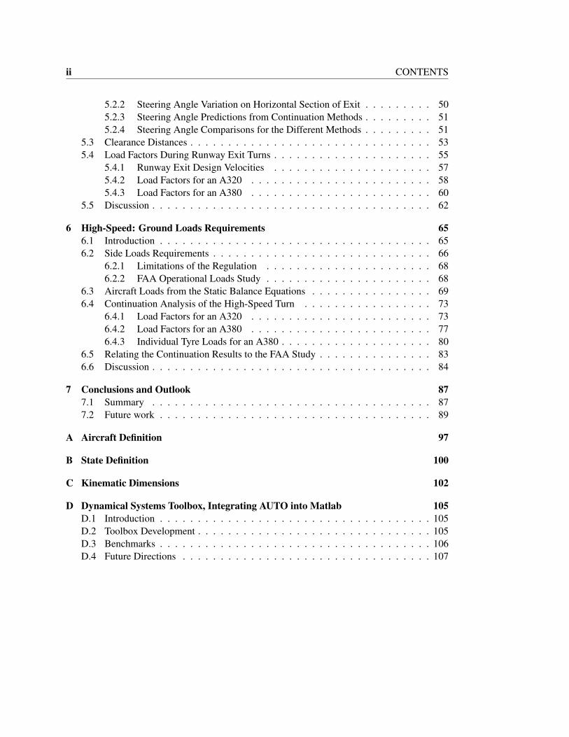
ii CONTENTS
5.2.2 Steering Angle Variation on Horizontal Section of Exit . . . . . . . . . 505.2.3 Steering Angle Predictions from Continuation Methods . . . . . . . . . 515.2.4 Steering Angle Comparisons for the Different Methods . . . . . . . . . 51
5.3 Clearance Distances . . . . . . . . . . . . . . . . . . . . . . . . . . . . . . . . 535.4 Load Factors During Runway Exit Turns . . . . . . . . . . . . . . . . . . . . . 55
5.4.1 Runway Exit Design Velocities . . . . . . . . . . . . . . . . . . . . . 575.4.2 Load Factors for an A320 . . . . . . . . . . . . . . . . . . . . . . . . 585.4.3 Load Factors for an A380 . . . . . . . . . . . . . . . . . . . . . . . . 60
5.5 Discussion . . . . . . . . . . . . . . . . . . . . . . . . . . . . . . . . . . . . . 62
6 High-Speed: Ground Loads Requirements 656.1 Introduction . . . . . . . . . . . . . . . . . . . . . . . . . . . . . . . . . . . . 656.2 Side Loads Requirements . . . . . . . . . . . . . . . . . . . . . . . . . . . . . 66
6.2.1 Limitations of the Regulation . . . . . . . . . . . . . . . . . . . . . . 686.2.2 FAA Operational Loads Study . . . . . . . . . . . . . . . . . . . . . . 68
6.3 Aircraft Loads from the Static Balance Equations . . . . . . . . . . . . . . . . 696.4 Continuation Analysis of the High-Speed Turn . . . . . . . . . . . . . . . . . 73
6.4.1 Load Factors for an A320 . . . . . . . . . . . . . . . . . . . . . . . . 736.4.2 Load Factors for an A380 . . . . . . . . . . . . . . . . . . . . . . . . 776.4.3 Individual Tyre Loads for an A380 . . . . . . . . . . . . . . . . . . . . 80
6.5 Relating the Continuation Results to the FAA Study . . . . . . . . . . . . . . . 836.6 Discussion . . . . . . . . . . . . . . . . . . . . . . . . . . . . . . . . . . . . . 84
7 Conclusions and Outlook 877.1 Summary . . . . . . . . . . . . . . . . . . . . . . . . . . . . . . . . . . . . . 877.2 Future work . . . . . . . . . . . . . . . . . . . . . . . . . . . . . . . . . . . . 89
A Aircraft Definition 97
B State Definition 100
C Kinematic Dimensions 102
D Dynamical Systems Toolbox, Integrating AUTO into Matlab 105D.1 Introduction . . . . . . . . . . . . . . . . . . . . . . . . . . . . . . . . . . . . 105D.2 Toolbox Development . . . . . . . . . . . . . . . . . . . . . . . . . . . . . . . 105D.3 Benchmarks . . . . . . . . . . . . . . . . . . . . . . . . . . . . . . . . . . . . 106D.4 Future Directions . . . . . . . . . . . . . . . . . . . . . . . . . . . . . . . . . 107
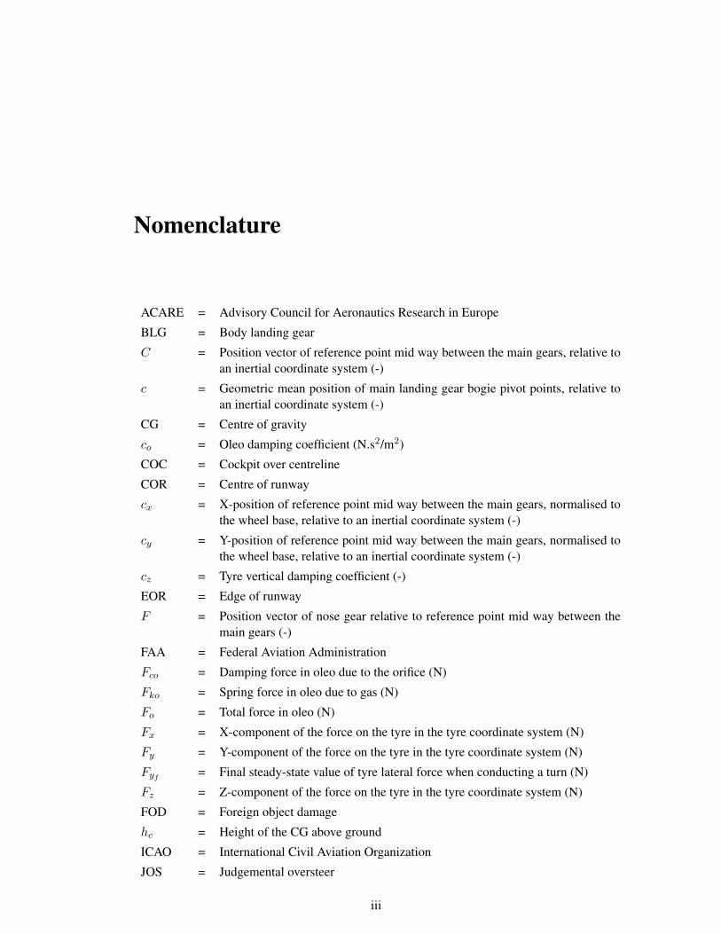
Nomenclature
ACARE = Advisory Council for Aeronautics Research in Europe
BLG = Body landing gear
C = Position vector of reference point mid way between the main gears, relative toan inertial coordinate system (-)
c = Geometric mean position of main landing gear bogie pivot points, relative toan inertial coordinate system (-)
CG = Centre of gravity
co = Oleo damping coefficient (N.s2/m2)
COC = Cockpit over centreline
COR = Centre of runway
cx = X-position of reference point mid way between the main gears, normalised tothe wheel base, relative to an inertial coordinate system (-)
cy = Y-position of reference point mid way between the main gears, normalised tothe wheel base, relative to an inertial coordinate system (-)
cz = Tyre vertical damping coefficient (-)
EOR = Edge of runway
F = Position vector of nose gear relative to reference point mid way between themain gears (-)
FAA = Federal Aviation Administration
Fco = Damping force in oleo due to the orifice (N)
Fko = Spring force in oleo due to gas (N)
Fo = Total force in oleo (N)
Fx = X-component of the force on the tyre in the tyre coordinate system (N)
Fy = Y-component of the force on the tyre in the tyre coordinate system (N)
Fyf = Final steady-state value of tyre lateral force when conducting a turn (N)
Fz = Z-component of the force on the tyre in the tyre coordinate system (N)
FOD = Foreign object damage
hc = Height of the CG above ground
ICAO = International Civil Aviation Organization
JOS = Judgemental oversteer
iii
iv CONTENTS
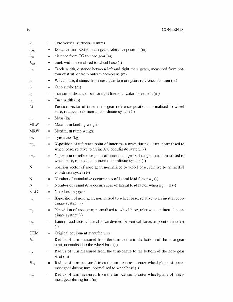
kz = Tyre vertical stiffness (N/mm)
lcm = Distance from CG to main gears reference position (m)
lcn = distance from CG to nose gear (m)
Lm = track width normalised to wheel base (-)
lm = Track width, distance between left and right main gears, measured from bot-tom of strut, or from outer wheel-plane (m)
ln = Wheel base, distance from nose gear to main gears reference position (m)
lo = Oleo stroke (m)
lt = Transition distance from straight line to circular movement (m)
ltw = Turn width (m)
M = Position vector of inner main gear reference position, normalised to wheelbase, relative to an inertial coordinate system (-)
m = Mass (kg)
MLW = Maximum landing weight
MRW = Maximum ramp weight
mt = Tyre mass (kg)
mx = X-position of reference point of inner main gears during a turn, normalised towheel base, relative to an inertial coordinate system (-)
my = Y-position of reference point of inner main gears during a turn, normalised towheel base, relative to an inertial coordinate system (-)
N = position vector of nose gear, normalised to wheel base, relative to an inertialcoordinate system (-)
N = Number of cumulative occurrences of lateral load factor ny (-)
N0 = Number of cumulative occurrences of lateral load factor when ny = 0 (-)
NLG = Nose landing gear
nx = X-position of nose gear, normalised to wheel base, relative to an inertial coor-dinate system (-)
ny = Y-position of nose gear, normalised to wheel base, relative to an inertial coor-dinate system (-)
ny = Lateral load factor: lateral force divided by vertical force, at point of interest(-)
OEM = Original equipment manufacturer
Rn = Radius of turn measured from the turn-centre to the bottom of the nose gearstrut, normalised to the wheel base (-)
rn = Radius of turn measured from the turn-centre to the bottom of the nose gearstrut (m)
Rm = Radius of turn measured from the turn-centre to outer wheel-plane of inner-most gear during turn, normalised to wheelbase (-)
rm = Radius of turn measured from the turn-centre to outer wheel-plane of inner-most gear during turn (m)
CONTENTS v
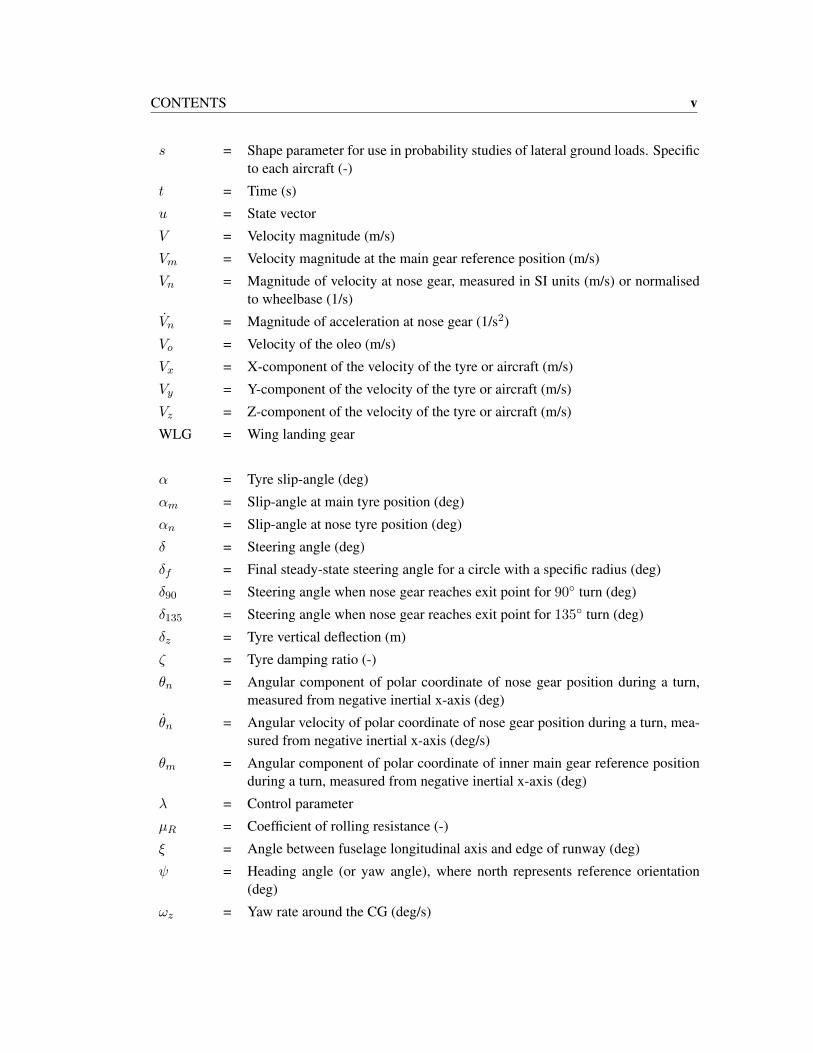
s = Shape parameter for use in probability studies of lateral ground loads. Specificto each aircraft (-)
t = Time (s)
u = State vector
V = Velocity magnitude (m/s)
Vm = Velocity magnitude at the main gear reference position (m/s)
Vn = Magnitude of velocity at nose gear, measured in SI units (m/s) or normalisedto wheelbase (1/s)
Vn = Magnitude of acceleration at nose gear (1/s2)
Vo = Velocity of the oleo (m/s)
Vx = X-component of the velocity of the tyre or aircraft (m/s)
Vy = Y-component of the velocity of the tyre or aircraft (m/s)
Vz = Z-component of the velocity of the tyre or aircraft (m/s)
WLG = Wing landing gear
α = Tyre slip-angle (deg)
αm = Slip-angle at main tyre position (deg)
αn = Slip-angle at nose tyre position (deg)
δ = Steering angle (deg)
δf = Final steady-state steering angle for a circle with a specific radius (deg)
δ90 = Steering angle when nose gear reaches exit point for 90◦ turn (deg)
δ135 = Steering angle when nose gear reaches exit point for 135◦ turn (deg)
δz = Tyre vertical deflection (m)
ζ = Tyre damping ratio (-)
θn = Angular component of polar coordinate of nose gear position during a turn,measured from negative inertial x-axis (deg)
θn = Angular velocity of polar coordinate of nose gear position during a turn, mea-sured from negative inertial x-axis (deg/s)
θm = Angular component of polar coordinate of inner main gear reference positionduring a turn, measured from negative inertial x-axis (deg)
λ = Control parameter
µR = Coefficient of rolling resistance (-)
ξ = Angle between fuselage longitudinal axis and edge of runway (deg)
ψ = Heading angle (or yaw angle), where north represents reference orientation(deg)
ωz = Yaw rate around the CG (deg/s)

Chapter 1
Introduction
1.1 Research Motivation and Objectives
The last century has seen huge strides in the progress of aviation, where the developmentof breakthrough technologies such as the metal wing, jet engines and fly-by-wire technolo-gies have given the companies developing these technologies a clear advantage. These game-changing technologies become even more pertinent when one looks at the General MarketForecast for aircraft that is published every two years by Airbus [4]. There it is shown that pas-senger numbers double every 15 years, with a consequent increased demand for new airframes.It is predicted that 24,000 new airframes will be needed by 2025 [4].
The Strategic Research Agenda [1] of the Advisory Council for Aeronautics Research in Eu-rope (ACARE) identifies the effects that such an increase in demand will have on the qualityand affordability of aircraft, the effect on the environment, safety, security and the efficiency ofthe air transport system. NASA has published a similar document in the form of the NationalPlan for Aeronautics Research and Development and Related Infrastructure [46]. Both reportshighlight similar challenges and identify the automation of aircraft movements, on the groundand in the air, as a means of meeting the objectives set out in these reports. Automation willincrease the throughput of aircraft at airports. It is envisaged that automation will enable theaircraft performance envelope to be safely enlarged, thereby giving the aircraft operators theability to customise their operations based on their market needs. Aircraft manufacturers arealso constantly striving to improve the efficiency of all aspects surrounding the operation oftheir aircraft. Obvious fuel savings can be made by decreasing the drag of the aircraft duringthe cruise phase. However, less obvious savings can be made by improving the way aircraftare operated on the ground. Recent studies indicate that efficiencies can be made if surfacemovements can be achieved through means other than that of the engines [5]. A large amountof fuel is consumed when an aircraft’s main engines are used to taxi around airports, where aforecasted total cost of fuel consumption during taxiing of around $7bn annually, is predictedby 2012 [5]. It is also predicted that this type of fuel consumption leads to CO2 emissions ofapproximately 18m tonnes per year, while Foreign Object Damage (FOD) contributes to a costof around $350m per year [5].
New operational procedures are also directed towards the reduction of noise, and taxiing conse-quently impacts the environment in terms of air and noise pollution. Several schemes for savingfuel on the ground have been proposed. The Taxibot [5] project is one such scheme, where the
1
2 Chapter 1. Introduction
engines are shut down and the pilot controls the movement of the aircraft on the ground viaa remotely controlled tug. New agile methods are needed to analyse novel architectures re-sulting from these new procedures, thus enabling the search of new optimal operating regimesfor the proposed architectures. The intended interactions amongst the Aircraft Architecturesand the Operational Environment Architectures are being envisioned and developed in projectssuch as NextGen [23] in the USA and CleanSky [20] in Europe. New competition from Japan,China, Russia and Brazil in the Single Aisle class of aircraft will only increase the need for newand innovative technologies, where the competitive advantage can be obtained by increasingand combining the functionality of the sub-systems, whilst lowering the development cost andimproving the operability of these systems. This is one reason why original equipment man-ufacturers (OEMs) such as Boeing and Airbus are putting greater focus on Architecting andIntegration roles, whilst seeking competitive advantages by utilizing the diversity that emergesthrough creating strategic partnerships in design and manufacturing [51].
Not only does automation address the goals of CleanSky, but it also increases the competitiveadvantage of the company that masters this skill. Examples of ground automation can alreadybe seen on aircraft such as the Airbus A380, which has incorporated two functions that cre-ate greater operational efficiencies for aircraft ground movements. The first is the Brake toVacate (BTV) function that reduces the time that the aircraft spends within the active area ofthe runway; and the second is the Heading Control Function (HCF), which ensures that the lastdemanded heading by the pilot is maintained [71]. In both cases, the crew workload is reduced,allowing them to concentrate on other more important tasks during the respective flight phase.Full automation on the ground is yet to be realised; the current sub-systems have only focussedon straight-line movement. Full automation will only be possible through a clear understand-ing of all the nonlinear effects that influence the lateral and yaw movement of the aircraft,especially during the turning phases of the aircraft on the ground.
Aeroplane characteristics manuals from the OEMs usually contain a baseline set of operatingprocedures that is used to demonstrate compatability with existing airport infrastructure. Thethree most common of these manoeuvres are the U-turn manoeuvre, an exit manoeuvre fromthe runway onto a taxiway, and the transition from one taxiway to another. There are severalways to conduct and interpret these manoeuvres due to the variability that is introduced by thepilot and the operating procedures of the airlines. A great deal of variance may exist in the waythat any of the ground manoeuvres is conducted, whether around the apron or during taxiing.This is due to the nonlinear nature of the landing gears [15], as well as the variance of theinputs from the pilot. A good example that highlights this variance can be found in the A380Airplane Characteristics Manual [2], which states:
“In the ground operating mode, varying airline practices may demand that moreconservative turning procedures be adopted to avoid excessive tyre wear and re-duce possible maintenance problems. Airline operating techniques will vary in thelevel of performance, over a wide range of operating circumstances throughout theworld. Variations from standard aircraft operating patterns may be necessary tosatisfy physical constraints within the maneuvering area, such as adverse grades,limited area or high risk of jet blast damage. For these reasons, ground maneu-vering requirements should be coordinated with the using airlines prior to layoutplanning”.
1.1. Research Motivation and Objectives 3
Landing gear engineers observe nonlinear phenomena such as hysteresis, backlash and stictionon a daily basis, without necessarily appreciating the full meaning behind these observations.A wheel that locks up during braking is a good example. Many conflicting requirements needto be considered during the design of a landing gear, where the weight and pavement load-ing need to be minimised, and the shock absorption maximised. The lateral stability on theground is determined by the position of the gears, along with the tyre and oleo (shock damper)characteristics. Experience has shown that the use of different tyres can mean the differencebetween a stable and an unstable aircraft. Landing gears contain highly nonlinear components,including tyres, brakes and oleos, and therefore traditional analysis is usually done at somevery specific design conditions. There is a perceived need to characterise the behaviour of thesystem over a wide variety of parameters, and this is the industrial domain where methods fromnonlinear dynamics can and should be brought to bear.
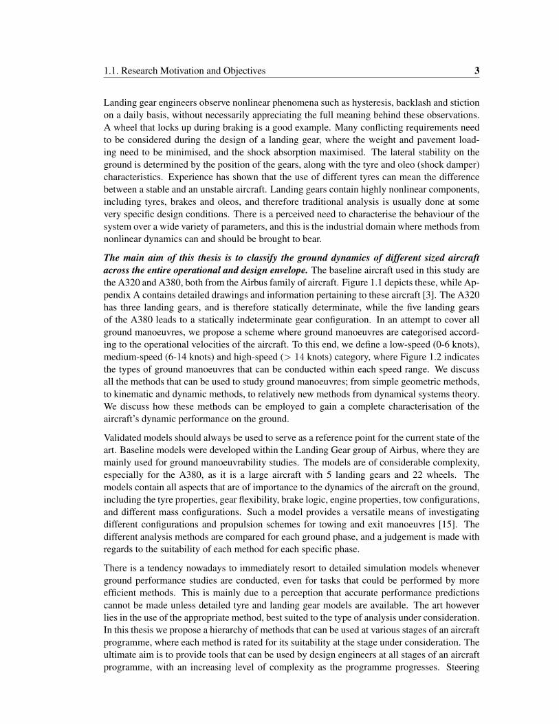
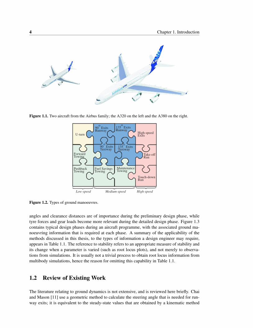
The main aim of this thesis is to classify the ground dynamics of different sized aircraftacross the entire operational and design envelope. The baseline aircraft used in this study arethe A320 and A380, both from the Airbus family of aircraft. Figure 1.1 depicts these, while Ap-pendix A contains detailed drawings and information pertaining to these aircraft [3]. The A320has three landing gears, and is therefore statically determinate, while the five landing gearsof the A380 leads to a statically indeterminate gear configuration. In an attempt to cover allground manoeuvres, we propose a scheme where ground manoeuvres are categorised accord-ing to the operational velocities of the aircraft. To this end, we define a low-speed (0-6 knots),medium-speed (6-14 knots) and high-speed (> 14 knots) category, where Figure 1.2 indicatesthe types of ground manoeuvres that can be conducted within each speed range. We discussall the methods that can be used to study ground manoeuvres; from simple geometric methods,to kinematic and dynamic methods, to relatively new methods from dynamical systems theory.We discuss how these methods can be employed to gain a complete characterisation of theaircraft’s dynamic performance on the ground.
Validated models should always be used to serve as a reference point for the current state of theart. Baseline models were developed within the Landing Gear group of Airbus, where they aremainly used for ground manoeuvrability studies. The models are of considerable complexity,especially for the A380, as it is a large aircraft with 5 landing gears and 22 wheels. Themodels contain all aspects that are of importance to the dynamics of the aircraft on the ground,including the tyre properties, gear flexibility, brake logic, engine properties, tow configurations,and different mass configurations. Such a model provides a versatile means of investigatingdifferent configurations and propulsion schemes for towing and exit manoeuvres [15]. Thedifferent analysis methods are compared for each ground phase, and a judgement is made withregards to the suitability of each method for each specific phase.
There is a tendency nowadays to immediately resort to detailed simulation models wheneverground performance studies are conducted, even for tasks that could be performed by moreefficient methods. This is mainly due to a perception that accurate performance predictionscannot be made unless detailed tyre and landing gear models are available. The art howeverlies in the use of the appropriate method, best suited to the type of analysis under consideration.In this thesis we propose a hierarchy of methods that can be used at various stages of an aircraftprogramme, where each method is rated for its suitability at the stage under consideration. Theultimate aim is to provide tools that can be used by design engineers at all stages of an aircraftprogramme, with an increasing level of complexity as the programme progresses. Steering
4 Chapter 1. Introduction
Figure 1.1. Two aircraft from the Airbus family; the A320 on the left and the A380 on the right.
U-turn
ForwardTowing
PushbackTowing
MaintenanceTowing
Fuel SavingsTowing
90o
ExitsRunway
135o
ExitsRunway
High-speedExits
Take-offRun
Touch-downRun
90o
ExitsTaxiway
135o
ExitsTaxiway
Low-speed Medium-speed High-speed
Figure 1.2. Types of ground manoeuvres.
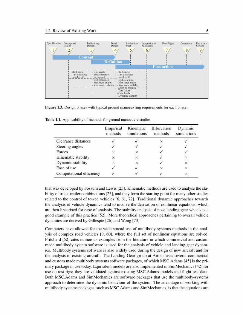
angles and clearance distances are of importance during the preliminary design phase, whiletyre forces and gear loads become more relevant during the detailed design phase. Figure 1.3contains typical design phases during an aircraft programme, with the associated ground ma-noeuvring information that is required at each phase. A summary of the applicability of themethods discussed in this thesis, to the types of information a design engineer may require,appears in Table 1.1. The reference to stability refers to an appropriate measure of stability andits change when a parameter is varied (such as root locus plots), and not merely to observa-tions from simulations. It is usually not a trivial process to obtain root locus information frommultibody simulations, hence the reason for omitting this capability in Table 1.1.
1.2 Review of Existing Work
The literature relating to ground dynamics is not extensive, and is reviewed here briefly. Chaiand Mason [11] use a geometric method to calculate the steering angle that is needed for run-way exits; it is equivalent to the steady-state values that are obtained by a kinematic method
1.2. Review of Existing Work 5
Specification
Concept
Definition
Production
ProductionStart
ConceptualDesign
PreliminaryDesign
DetailDesign
Integration &Validation
First Flight Operations
1 2 4 5 6 7 8 93
- Roll-angle- Tail-clearance
at take-off
- Roll-angle- Tail-clearance
at take-off- Exit clearance- Max steer angles- Kinematic stability
- Roll-angle- Tail-clearance
at take-off- Exit clearance- Max steer angles
- Steering torques- Tyre forces- Gear loads- Dynamic stability
- Kinematic stability
Entry IntoService
Figure 1.3. Design phases with typical ground manoeuvring requirements for each phase.
Table 1.1. Applicability of methods for ground manoeuvre studies
Empirical Kinematic Bifurcation Dynamicmethods simulations methods simulations
Clearance distances X X × XSteering angles X X X XForces × × X XKinematic stability × × X ×Dynamic stability × × X ×Ease of use X X × ×Computational efficiency X X X ×
that was developed by Fossum and Lewis [25]. Kinematic methods are used to analyse the sta-bility of truck-trailer combinations [25], and they form the starting point for many other studiesrelated to the control of towed vehicles [6, 61, 72]. Traditional dynamic approaches towardsthe analysis of vehicle dynamics tend to involve the derivation of nonlinear equations, whichare then linearised for ease of analysis. The stability analysis of nose landing gear wheels is agood example of this practice [52]. More theoretical approaches pertaining to overall vehicledynamics are derived by Gillespie [26] and Wong [73].
Computers have allowed for the wide-spread use of multibody systems methods in the anal-ysis of complex road vehicles [9, 60], where the full set of nonlinear equations are solved.Pritchard [52] cites numerous examples from the literature in which commercial and custommade multibody system software is used for the analysis of vehicle and landing gear dynam-ics. Multibody systems software is also widely used during the design of new aircraft and forthe analysis of existing aircraft. The Landing Gear group at Airbus uses several commercialand custom made multibody systems software packages, of which MSC.Adams [45] is the pri-mary package in use today. Equivalent models are also implemented in SimMechanics [42] foruse on test rigs; they are validated against existing MSC.Adams models and flight test data.Both MSC.Adams and SimMechanics are software packages that use the multibody-systemsapproach to determine the dynamic behaviour of the system. The advantage of working withmultibody systems packages, such as MSC.Adams and SimMechanics, is that the equations are
6 Chapter 1. Introduction
automatically derived; hence, an environment is created where the engineers can focus on theengineering aspects of the task in hand, and not necessarily on the derivation of the equationsof motion. Such packages provide a complete framework within which models can be builtand simulated. Multibody models are not only used for simulations, but also for bifurcationanalysis, as is demonstrated in this thesis.
Thota et al. [64] showed how nonlinear geometric effects have a significant influence on theonset of nose gear vibrations. Tyres create the most significant nonlinear effects in traditionalroad vehicles [50], and similar effects were found in aircraft tyres at low velocities [13, 54,55]. Klyde et al. [33] conducted specific ground tests to evaluate aircraft ground handlingcharacteristics. They showed that the aerodynamic effects are far more significant in aircraftat high velocities, when compared to cars [35]. The effect of tyre pressure on ground handlingwas also investigated in [34], as well as an assessment of the effectiveness of an augmentedsteering system [36]. Nonlinear models are also used to a great extent in the area of flightmechanics, where Thompson and McMillan [63] provide an overview of their use.
Bifurcation analysis has been used successfully to study the longitudinal motion of low-orderroad vehicle models with periodic forcing [75] and driver feedback control [39, 40]. Steady-state behaviour, periodic motions and chaotic dynamics were found in these models. The lateraldynamics of road vehicles were studied by Nguyen et al. [48, 49, 70], and they showed that theentry into a spin can be associated with a bifurcation point, indicating a loss of stability.
The first application of bifurcation and continuation methods in aerospace, was in the area offlight mechanics [43], and it is now used as an effective tool for the study of nonlinear phe-nomena in aerospace vehicles. Some examples in the field of flight mechanics can be foundin [12, 41], where the aerodynamics creates the dominant nonlinear effects. Bifurcation meth-ods have also been identified by NASA as a key technology for the analysis of aircraft flightdynamics in off-nominal conditions [38], in other words, during upset conditions. Bifurca-tion and continuation techniques have been used to study nose gear vibrations (also knownas wheel shimmy) during straight-line aircraft motion, using low-order mathematical mod-els [64, 65, 66, 67, 68].
The application of bifurcation and continuation methods, to study an aircraft turning on theground, is still quite a new subject. The original research in this area was done by the authorfor his Master’s thesis [13], which was the first practical demonstration of the usefulness ofbifurcation methods for the study of aircraft ground manoeuvres. Further studies by JamesRankin identified safe ground operating regions for the A320, with the accompanying modesthat lead to a loss of control [54, 55]. These studies used industrially developed models and asimplified mathematical model [55, 56]. This thesis expands on the statically determinate geararrangement of the A320 by analysing different ground manoeuvres and additional mass cases.The bifurcation analysis of an aircraft with a statically indeterminate gear arrangement — theA380 — is new to the field, as is the identification and comparison of the different methodsthat can be used to analyse ground manoeuvres. The advantages of these methods are that theyproduce a complete picture of the dynamics in all operating regions, and at a fraction of thecost of simulations.
It is known that the current regulation for high-speed turns is very conservative for large air-craft [57], and consequently the Federal Aviation Administration (FAA) conducted a measure-ment campaign of the operational loads that an aircraft may experience during normal opera-tions. The aim of this campaign was to identify the factors that affect the operational loads, and

1.3. Thesis Overview 7
to assess the existing certification criteria [57, 58, 59]. A further study by the FAA [69] com-pares the operational loads for a range of different sized aircraft, and showed that the lateralload factor is reduced when the size of the aircraft is increased. Empirical formulae were de-rived to calculate the statistical probability of certain load factors. The statistics for the taxi-inphase showed larger lateral load factors than the taxi-out phase, and it was recognised that cor-rections were needed to account for the change in the aircraft weight during the taxi-in phase.Another FAA study [32] was conducted to account for this weight change. Specific groundtests were also conducted to address concerns that were highlighted in the previous studies,where Finn et al. [24] performed ground tests to find the maximum lateral loads at individuallanding gears. The use of the A320 and A380 models allows us to assess the validity of theseformulae. It also allows for the identification of the main factors that reduce the lateral loadfactor with an increase in size. Rankin et al. [56] conducted simulations to ascertain the max-imum load factors that could be obtained at runway exits. The results suggest that the limitimposed in the Federal Airworthiness Regulation (FAR) is conservative for the main landinggears and possibly not stringent enough for the nose landing gear.
1.3 Thesis Overview
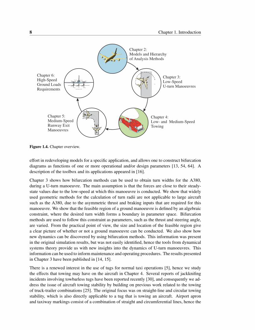
This thesis covers the most widely used operational procedures that are conducted on an aircraftduring ground movements, either under its own power or by means of a tug. The chaptersfollow from the types of manoeuvres that are identified in Figure 1.2, where the chapters areordered to start from low-speed U-turn manoeuvres, building up to high-speed turns. Figure 1.4contains an overview of the different chapters. The size of an aircraft has a significant influenceon the dynamics of an aircraft on the ground. The dynamics of an aircraft with three landinggears, such as the A320, has different dynamics than an aircraft such as the A380, which hasfive landing gears. The analysis in each chapter will highlight these differences.
In Chapter 2 we discuss the most widely employed analysis methods that can be used tostudy aircraft ground manoeuvres. The first is a kinematic method that was originally devel-oped for jackknifing studies [25]; it is suitable for clearance and steering angle investigations.The second method makes use of simulations, and shows how models are constructed in theMSC.Adams and SimMechanics software environments; all relevant information in terms ofsteering angles, clearance distances, and tyre forces are provided. We also discuss how themodels are validated. Good agreement is shown between the simulation results and flight test1
data, underpinning the validity of the models, making them suitable for ground manoeuvrestudies. The computational challenges related to multibody simulations are also highlighted.The models presented in this chapter have been published in [14, 15]. The final method isbased on bifurcation and continuation methods; it can be used to obtain turn radii, or steady-state forces on any gear or tyre. To allow for the nonlinear analysis of industrially-tested modelsin a user-friendly environment, AUTO [19] has been integrated with Matlab in the form of aDynamical Systems Toolbox. The SimMechanics models are coupled to AUTO within this newtoolbox, where AUTO has direct access to the states of the SimMechanics model, even thoughthe model equations are a black-box to the user. This is an important capability that allowsone to integrate existing validated models with the bifurcation software, avoiding significant
1Ground tests are also classified as flight tests.
8 Chapter 1. Introduction
0.5VM2
0.5VN
0.5VM1
VM2
VM1
NOSE WHEEL TYPE
0.5W W
Chapter 2:Models and Hierarchyof Analysis Methods
Chapter 3:Low-SpeedU-turn Manoeuvres
Chapter 4:Low- and Medium-SpeedTowing
Chapter 5:Medium-SpeedRunway ExitManoeuvres
Chapter 6:High-SpeedGround LoadsRequirements
Figure 1.4. Chapter overview.
effort in redeveloping models for a specific application, and allows one to construct bifurcationdiagrams as functions of one or more operational and/or design parameters [13, 54, 64]. Adescription of the toolbox and its applications appeared in [16].
Chapter 3 shows how bifurcation methods can be used to obtain turn widths for the A380,during a U-turn manoeuvre. The main assumption is that the forces are close to their steady-state values due to the low-speed at which this manoeuvre is conducted. We show that widelyused geometric methods for the calculation of turn radii are not applicable to large aircraftsuch as the A380, due to the asymmetric thrust and braking inputs that are required for thismanoeuvre. We show that the feasible region of a ground manoeuvre is defined by an algebraicconstraint, where the desired turn width forms a boundary in parameter space. Bifurcationmethods are used to follow this constraint as parameters, such as the thrust and steering angle,are varied. From the practical point of view, the size and location of the feasible region givea clear picture of whether or not a ground manoeuvre can be conducted. We also show hownew dynamics can be discovered by using bifurcation methods. This information was presentin the original simulation results, but was not easily identified, hence the tools from dynamicalsystems theory provide us with new insights into the dynamics of U-turn manoeuvres. Thisinformation can be used to inform maintenance and operating procedures. The results presentedin Chapter 3 have been published in [14, 15].
There is a renewed interest in the use of tugs for normal taxi operations [5], hence we studythe effects that towing may have on the aircraft in Chapter 4. Several reports of jackknifingincidents involving towbarless tugs have been reported recently [30], and consequently we ad-dress the issue of aircraft towing stability by building on previous work related to the towingof truck-trailer combinations [25]. The original focus was on straight-line and circular towingstability, which is also directly applicable to a tug that is towing an aircraft. Airport apronand taxiway markings consist of a combination of straight and circumferential lines, hence the
1.3. Thesis Overview 9
analysis of straight and circular manoeuvres is adequate. We do not derive the proofs for sta-bility, as this was done by Fossum and Lewis [25]. We do however show all the different waysin which jackknifing may occur. An aircraft that is towed in a forward direction is inherentlystable, while an aircraft that is being pushed back is inherently unstable. We also show thatan aircraft will converge to a stable circular movement when the nose gear trajectory is largerthan its wheel base when it being towed, while jackknifing will occur when the towing radiusis smaller than the wheel base. We use the results from a continuation analysis to determine theeffects that towing has when compared to when the aircraft moves under its own power. In thisway, we show that the forces on the aft-axles of the body gears are significantly higher whenthe aircraft is being towed; this is offset by lower forces on other parts of the gears.
In Chapter 5 we show that an exit manoeuvre is essentially a transition from a straight line toa circular trajectory, where the shape of the steering angle curve forms an exponential functionthat eventually settles into a steady-state value. This is contrary to previous approaches wherea ramp input is assumed [56]. The kinematic method is used for the initial analysis of runwayexit manoeuvres; it is however still deemed to be a difficult method for everyday use. Thereforeempirical formulae for the steering angle variation are derived. The strength of these formulaelie in their validity for any aircraft configuration. A comparison is made between the empirical,kinematic, and dynamic methods, where we conclude that the empirical and kinematic methodsare sufficient to predict the steering angle variation for a towed case, while a minor adjustmentis needed for the self-propelled case. Empirical equations are also derived for the minimumclearance distances that can be expected for 90◦ and 135◦ exits. A comparison is again madebetween the empirical, kinematic, and dynamic methods, where it is shown that the differencein the clearance predictions from the different methods are negligible. A diagram that indicatesthe feasibility of exit manoeuvres at Group V and VI airports is then constructed for any aircraftconfiguration; it gives valuable insight into the effects of wheel base and track width on theclearance distances for specific configurations. This diagram can be used as an effective toolfor design purposes. The last part of the chapter studies the dynamic forces that are generatedduring runway exit manoeuvres. Symmetric thrust with no braking is assumed. The resultsshow that the dynamic force values at the main gears are approximately 10% larger than thesteady-state values for the A320, and that the steady-state values are in fact the maximumvalues that can be obtained for the A380. Continuation methods can therefore be used toobtain the loads at the gears and the tyres for exit manoeuvres. The analysis methods andresults presented in Chapter 5 have been published in [14, 15].
In Chapter 6 we study the loads that can be generated during a high-speed turn. The originallateral ground loads requirement for an aircraft during a high-speed turn was written in themiddle of the last century, and consequently it is felt that this requirement is conservativewhen applied to large modern passenger aircraft [69]; the results from a operational loadsmeasurement campaign support this statement [69]. We assess the loads that can be generatedby an A320 and an A380, and compare the results to the original requirement. We show thatstatic balance equations and continuation methods can be used to assess the loads. Comparisonsare made between the two aircraft types, and they show significantly different dynamics interms of stability and loads. Symmetric thrust with no braking is once again assumed. Hopfbifurcations indicate a loss of stability for the A320 [13, 54, 55], while no bifurcations weredetected for the A380. The results for the A380 do however show that the nose gear tyresoperate close to a lateral load saturation point above certain velocities. An increase of thesteering angle has no effect on the turn radius above the value where the saturation occurs, and
10 Chapter 1. Introduction
consequently the radius stays close to a constant value above this saturation value. We showa strong correlation between the results from continuation analysis and the results from themeasurement campaign, and explain how an A320 can possibly obtain the lateral loads valuesthat were observed in the test campaign. The A380 can only generate a load that is half the valuestipulated by the requirement. This is due to the nonlinear nature of the tyre properties andthe overwhelming influence of the aerodynamics at high velocities. This provides additionalevidence that a lateral load factor of 0.5 cannot be reached for such a large aircraft.
In Chapter 7 we present a summary of our findings and outline directions for future work.
Chapter 2
Models and Hierarchy of Analysis Methods
2.1 Introduction
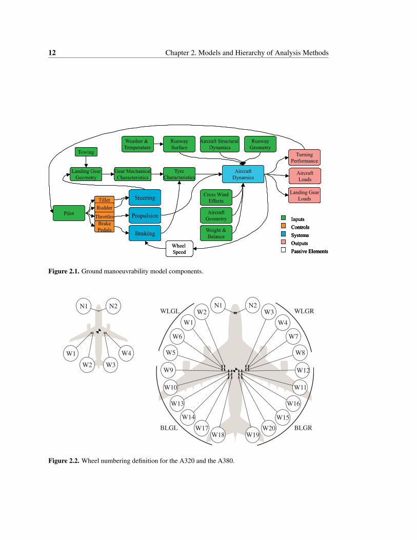
Ground manoeuvre predictions are usually made with advanced modelling and simulation tech-nologies, and they form an invaluable tool within the design process. They are used for detailedperformance predictions to test aircraft manoeuvrability under normal and abnormal condi-tions, as well as the definition of towing procedures for operators. Detailed models that containall the physical characteristics of the landing gears and tyres are used to analyse the dynamicsof an aircraft on the ground. The results from the simulations are used to obtain clearancedistances, steering angles, forces on the tyres and gears, and many other parameters of interest.
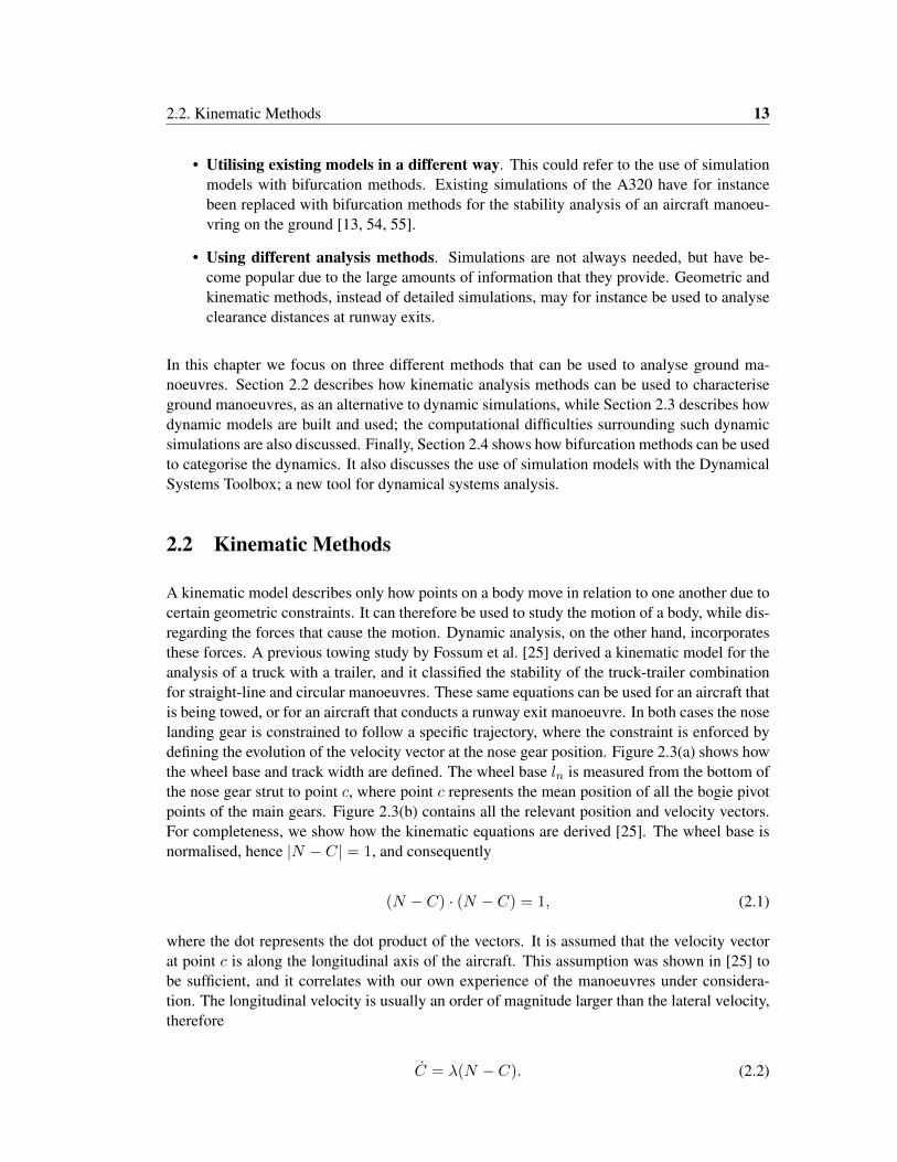
Validated models and methods therefore form the basis of the predictions. Figure 2.1 containsa schematic of typical components within an aircraft ground manoeuvrability model. In thisstudy we use validated SimMechanics models of the A320 and the A380 [13, 15, 54, 55]. TheA320 consists of three landing gears; one nose gear, and two main gears that are attached to thewings. Each gear has an axle with two wheels. The A380 has five landing gears; one nose gear,two main gears attached to the wings, and two main gears attached to the fuselage. Each winglanding gear (WLG) consists of a bogie with four wheels on each gear, while each body landinggear (BLG) consists of a bogie with six wheels. The aft axle of each BLG is steered. Six tyresare therefore present in the case of the A320 model, and 22 tyres in the A380 model. Figure 2.2contains the numbering conventions of the wheels for both the A320 and A380 models.
Despite all the advantages that simulations bring, there are drawbacks related to the run-timesof such simulations, the skills that are needed by specialist engineers to build satisfactory mod-els, as well as the availability of data during the early design phases. The costs related todynamic simulations make it necessary to evaluate all the different analysis techniques that canbe used for the specific problem at hand. The following approaches can be followed if the aimis to reduce the analysis time:
• Reduction of computational run-times. This can either be achieved by using morepowerful computational resources, or by focussing on more efficient algorithms. Re-cent work on the reformulation of the equations of motion by Udwadia and Kalaba [18]promises to ease the construction of the underlying equations, as well as provide im-provements in the run-times.
11
12 Chapter 2. Models and Hierarchy of Analysis Methods
Inputs
Controls
Systems
Outputs
Passive Elements
Tyre
Characteristics
Aircraft
Dynamics
Turning
Performance
Aircraft
Loads
Landing Gear
LoadsCross Wind
Effects
Runway
Geometry
Runway
Surface
Weather &
Temperature
Weight &
Balance
Aircraft
Geometry
Landing Gear
Geometry
Gear Mechanical
Characteristics
Pilot PropulsionThrottles
Rudder
Tiller
Brake
PedalsBraking
Steering
Wheel
Speed
Aircraft Structural
DynamicsTowing
Inputs
Controls
Systems
Outputs
Passive Elements
InputsInputs
ControlsControls
SystemsSystems
OutputsOutputs
Passive ElementsPassive Elements
Tyre
Characteristics
Aircraft
Dynamics
Turning
Performance
Aircraft
Loads
Landing Gear
LoadsCross Wind
Effects
Runway
Geometry
Runway
Surface
Weather &
Temperature
Weight &
Balance
Aircraft
Geometry
Landing Gear
Geometry
Gear Mechanical
Characteristics
Pilot PropulsionThrottles
Rudder
Tiller
Brake
Pedals
Throttles
Rudder
Tiller
Brake
PedalsBraking
Steering
Wheel
Speed
Aircraft Structural
DynamicsTowing
Figure 2.1. Ground manoeuvrability model components.
W1
N1 N2
W4
W2 W3
N1 N2
W4
W7
W1
W6
W2 W3
W12
W11
W16
W15
W20
W19
W13
W14
W17
W18
W9
W10
W5 W8
BLGL BLGR
WLGL WLGR
Figure 2.2. Wheel numbering definition for the A320 and the A380.
2.2. Kinematic Methods 13
• Utilising existing models in a different way. This could refer to the use of simulationmodels with bifurcation methods. Existing simulations of the A320 have for instancebeen replaced with bifurcation methods for the stability analysis of an aircraft manoeu-vring on the ground [13, 54, 55].
• Using different analysis methods. Simulations are not always needed, but have be-come popular due to the large amounts of information that they provide. Geometric andkinematic methods, instead of detailed simulations, may for instance be used to analyseclearance distances at runway exits.
In this chapter we focus on three different methods that can be used to analyse ground ma-noeuvres. Section 2.2 describes how kinematic analysis methods can be used to characteriseground manoeuvres, as an alternative to dynamic simulations, while Section 2.3 describes howdynamic models are built and used; the computational difficulties surrounding such dynamicsimulations are also discussed. Finally, Section 2.4 shows how bifurcation methods can be usedto categorise the dynamics. It also discusses the use of simulation models with the DynamicalSystems Toolbox; a new tool for dynamical systems analysis.
2.2 Kinematic Methods
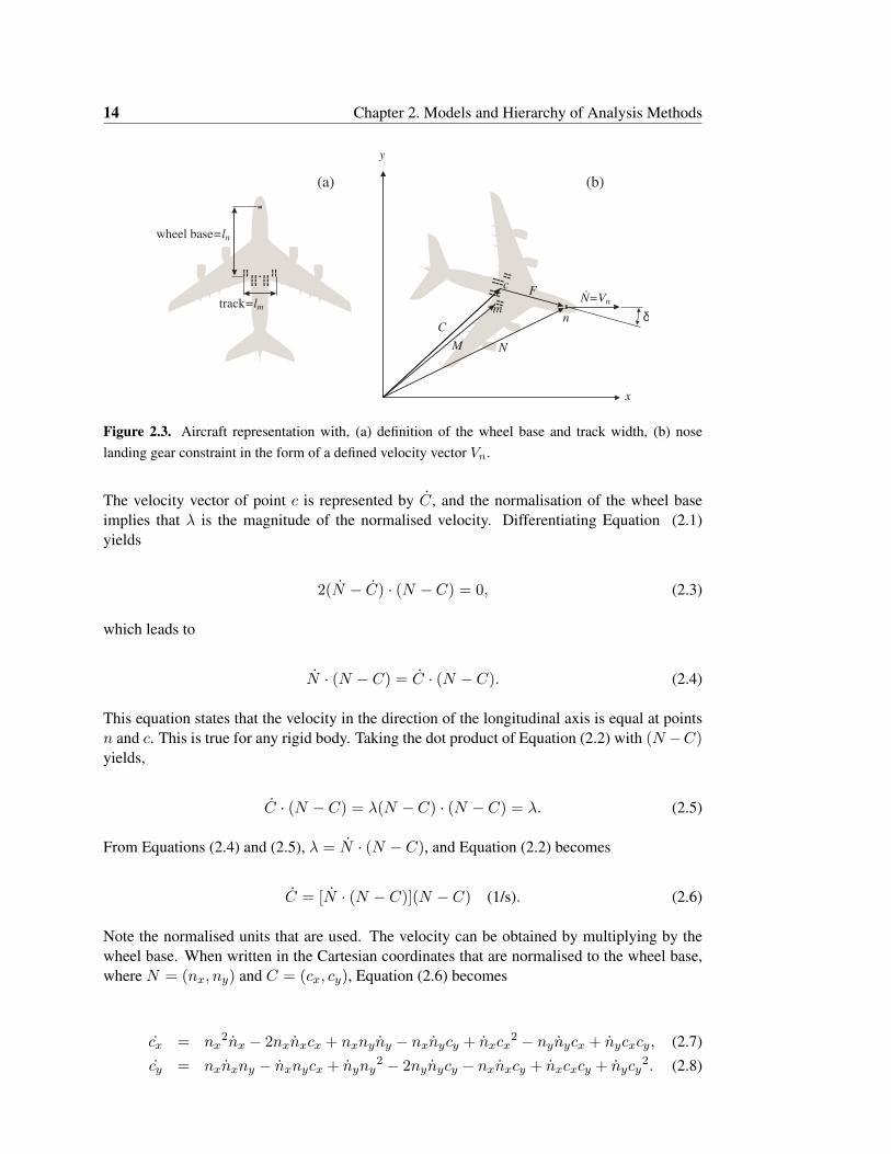
A kinematic model describes only how points on a body move in relation to one another due tocertain geometric constraints. It can therefore be used to study the motion of a body, while dis-regarding the forces that cause the motion. Dynamic analysis, on the other hand, incorporatesthese forces. A previous towing study by Fossum et al. [25] derived a kinematic model for theanalysis of a truck with a trailer, and it classified the stability of the truck-trailer combinationfor straight-line and circular manoeuvres. These same equations can be used for an aircraft thatis being towed, or for an aircraft that conducts a runway exit manoeuvre. In both cases the noselanding gear is constrained to follow a specific trajectory, where the constraint is enforced bydefining the evolution of the velocity vector at the nose gear position. Figure 2.3(a) shows howthe wheel base and track width are defined. The wheel base ln is measured from the bottom ofthe nose gear strut to point c, where point c represents the mean position of all the bogie pivotpoints of the main gears. Figure 2.3(b) contains all the relevant position and velocity vectors.For completeness, we show how the kinematic equations are derived [25]. The wheel base isnormalised, hence |N − C| = 1, and consequently
(N − C) · (N − C) = 1, (2.1)
where the dot represents the dot product of the vectors. It is assumed that the velocity vectorat point c is along the longitudinal axis of the aircraft. This assumption was shown in [25] tobe sufficient, and it correlates with our own experience of the manoeuvres under considera-tion. The longitudinal velocity is usually an order of magnitude larger than the lateral velocity,therefore
C = λ(N − C). (2.2)
14 Chapter 2. Models and Hierarchy of Analysis Methods
x
y
N
C
Ftrack=lm
wheel base=ln
δn
c
(a) (b)
m
M
N=Vn
Figure 2.3. Aircraft representation with, (a) definition of the wheel base and track width, (b) noselanding gear constraint in the form of a defined velocity vector Vn.
The velocity vector of point c is represented by C, and the normalisation of the wheel baseimplies that λ is the magnitude of the normalised velocity. Differentiating Equation (2.1)yields
2(N − C) · (N − C) = 0, (2.3)
which leads to
N · (N − C) = C · (N − C). (2.4)
This equation states that the velocity in the direction of the longitudinal axis is equal at pointsn and c. This is true for any rigid body. Taking the dot product of Equation (2.2) with (N −C)yields,
C · (N − C) = λ(N − C) · (N − C) = λ. (2.5)
From Equations (2.4) and (2.5), λ = N · (N − C), and Equation (2.2) becomes
C = [N · (N − C)](N − C) (1/s). (2.6)
Note the normalised units that are used. The velocity can be obtained by multiplying by thewheel base. When written in the Cartesian coordinates that are normalised to the wheel base,where N = (nx, ny) and C = (cx, cy), Equation (2.6) becomes
cx = nx2nx − 2nxnxcx + nxnyny − nxnycy + nxcx
2 − nynycx + nycxcy, (2.7)
cy = nxnxny − nxnycx + nyny2 − 2nynycy − nxnxcy + nxcxcy + nycy
2. (2.8)
2.3. Dynamic Methods - Modelling and Simulation 15
The angle δ represents the steering angle, or the angle between the longitudinal axis of theaircraft and the longitudinal axis of the tug, and is given by
δ = cos−1
(N · (N − C)
|N |
). (2.9)
A steering angle of zero indicates that the nose gear axle is perpendicular to the longitudinalaxes of the aircraft. In Chapter 3 we will show how kinematic methods can be used for theanalysis of towing stability, and in Chapter 5 kinematic methods are used for steering angleand clearance distance predictions.
2.3 Dynamic Methods - Modelling and Simulation
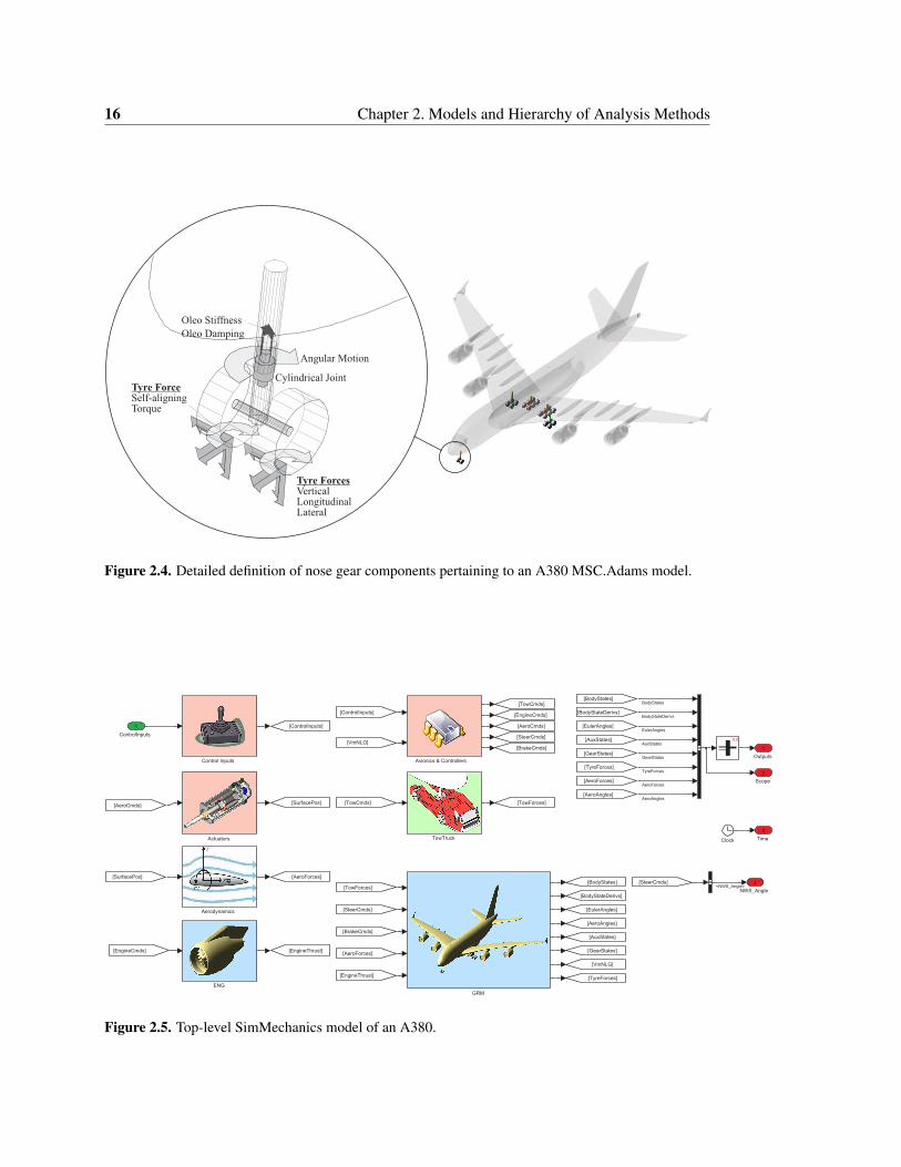
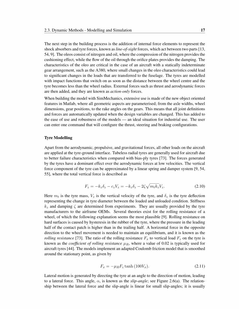
The models that are used at Airbus are built with different test platforms in mind. MSC.Adamsmodels are used for detailed ground manoeuvrability studies, while SimMechanics modelsare used on the test rigs, where the real-time performance of the models is critical. TheMSC.Adams environment is user-friendly and is the preferred model development environ-ment. MSC.Adams models are then converted to SimMechanics for testing with the avionicsthat will be implemented on the aircraft. Figure 2.4 shows a typical MSC.Adams model of theA380, with a specific focus on the nose landing gear, while Figure 2.5 contains the SimMe-chanics representation. Similar models exist for the A320 and are used in exactly the sameway. The following sections show how the models are constructed and used. Chapters 3, 5 and6 show how simulations are used for the analysis of ground manoeuvres.
2.3.1 Model Construction
The first step in the model building process is to describe the rigid parts and the joints connect-ing the parts [9], where a part is described by its mass, inertia and orientation. A right-handedcoordinate axis system is used. From a pilot’s perspective, the x-axis is in the forward directionalong the fuselage, the y-axis to the right, and the z-axis downward. The same (local) coor-dinate system is used for the tyres. The calculation of the aerodynamic angles of the aircraft,and the slip-angles on the tyres are straightforward when these conventions are used for thelocal coordinate systems. The nose gear is constrained by a cylindrical joint, which is drivenby an angular motion, as depicted in Figure 2.4. Each type of joint has a number of associateddegrees of freedom. For instance, a prismatic joint represents one degree of freedom (lineartranslation). Two states are present, namely a translational displacement and a translationalvelocity. A cylindrical joint contains a translational and rotational degree of freedom, hencefour states. Torsional flexibility of the shock absorber (also known as an oleo) is importantfor a landing gear with a bogie. Consequently, the oleos of the A380 model contain rotationaljoints that are constrained by rotational springs, representing the stiffness of the torque link.The aft-axle steering inputs are inserted as motions from a control law. Table B.1 in AppendixB contains a list of the components with the constraints (and states) associated with each com-ponent for the Airbus A320 and A380 aircraft. The A320 model contains a total of 18 states,and the A380 model contains 38 states.
16 Chapter 2. Models and Hierarchy of Analysis Methods
Cylindrical Joint
Angular Motion
Oleo Stiffness
Oleo Damping
Tyre ForceSelf-aligningTorque
Tyre ForcesVerticalLongitudinalLateral
Figure 2.4. Detailed definition of nose gear components pertaining to an A380 MSC.Adams model.
0:0
Figure 2.5. Top-level SimMechanics model of an A380.
2.3. Dynamic Methods - Modelling and Simulation 17
The next step in the building process is the addition of internal force elements to represent theshock absorbers and tyre forces, known as line-of-sight forces, which act between two parts [13,54, 9]. The oleos consist of nitrogen and oil, where the compression of the nitrogen provides thecushioning effect, while the flow of the oil through the orifice plates provides the damping. Thecharacteristics of the oleo are critical in the case of an aircraft with a statically indeterminategear arrangement, such as the A380, where small changes in the oleo characteristics could leadto significant changes in the loads that are transferred to the fuselage. The tyres are modelledwith impact functions that switch on as soon as the distance between the wheel centre and thetyre becomes less than the wheel radius. External forces such as thrust and aerodynamic forcesare then added, and they are known as action-only forces.
When building the model with SimMechanics, extensive use is made of the new object orientedfeatures in Matlab, where all geometric aspects are parameterised; from the axle widths, wheeldimensions, gear positions, to the rake angles on the gears. This means that all joint definitionsand forces are automatically updated when the design variables are changed. This has added tothe ease of use and robustness of the models — an ideal situation for industrial use. The usercan enter one command that will configure the thrust, steering and braking configurations.
Tyre Modelling
Apart from the aerodynamic, propulsive, and gravitational forces, all other loads on the aircraftare applied at the tyre-ground interface. Tubeless radial tyres are generally used for aircraft dueto better failure characteristics when compared with bias-ply tyres [73]. The forces generatedby the tyres have a dominant effect over the aerodynamic forces at low velocities. The verticalforce component of the tyre can be approximated by a linear spring and damper system [9, 54,55], where the total vertical force is described as
Fz = −kzδz − czVz = −kzδz − 2ζ√mtkzVz. (2.10)
Here mt is the tyre mass, Vz is the vertical velocity of the tyre, and δz is the tyre deflectionrepresenting the change in tyre diameter between the loaded and unloaded condition. Stiffnesskz and damping ζ are determined from experiments. They are usually provided by the tyremanufacturers to the airframe OEMs. Several theories exist for the rolling resistance of awheel, of which the following explanation seems the most plausible [9]. Rolling resistance onhard surfaces is caused by hysteresis in the rubber of the tyre, where the pressure in the leadinghalf of the contact patch is higher than in the trailing half. A horizontal force in the oppositedirection to the wheel movement is needed to maintain an equilibrium, and it is known as therolling resistance [73]. The ratio of the rolling resistance Fx to vertical load Fz on the tyre isknown as the coefficient of rolling resistance µR, where a value of 0.02 is typically used foraircraft tyres [44]. The models implement an adapted Coulomb friction model that is smoothedaround the stationary point, as given by
Fx = −µRFz tanh (100Vx). (2.11)
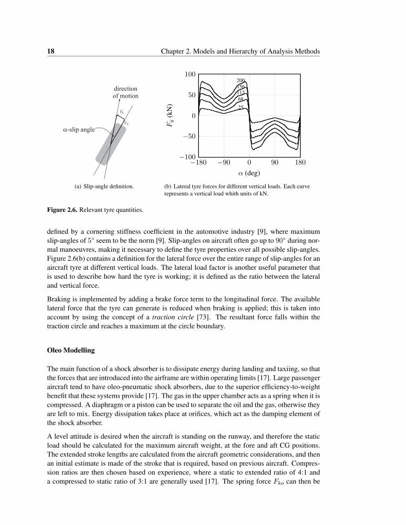
Lateral motion is generated by directing the tyre at an angle to the direction of motion, leadingto a lateral force. This angle, α, is known as the slip-angle; see Figure 2.6(a). The relation-ship between the lateral force and the slip-angle is linear for small slip-angles; it is usually
18 Chapter 2. Models and Hierarchy of Analysis Methods
Vy
Vx
directionof motion
a-slip angle
(a) Slip-angle definition.
−180 −90 0 90 180−100
−50
0
50
100
25
68112156200
α (deg)Fy
(kN
)
(b) Lateral tyre forces for different vertical loads. Each curverepresents a vertical load whith units of kN.
Figure 2.6. Relevant tyre quantities.
defined by a cornering stiffness coefficient in the automotive industry [9], where maximumslip-angles of 5◦ seem to be the norm [9]. Slip-angles on aircraft often go up to 90◦ during nor-mal manoeuvres, making it necessary to define the tyre properties over all possible slip-angles.Figure 2.6(b) contains a definition for the lateral force over the entire range of slip-angles for anaircraft tyre at different vertical loads. The lateral load factor is another useful parameter thatis used to describe how hard the tyre is working; it is defined as the ratio between the lateraland vertical force.
Braking is implemented by adding a brake force term to the longitudinal force. The availablelateral force that the tyre can generate is reduced when braking is applied; this is taken intoaccount by using the concept of a traction circle [73]. The resultant force falls within thetraction circle and reaches a maximum at the circle boundary.
Oleo Modelling
The main function of a shock absorber is to dissipate energy during landing and taxiing, so thatthe forces that are introduced into the airframe are within operating limits [17]. Large passengeraircraft tend to have oleo-pneumatic shock absorbers, due to the superior efficiency-to-weightbenefit that these systems provide [17]. The gas in the upper chamber acts as a spring when it iscompressed. A diaphragm or a piston can be used to separate the oil and the gas, otherwise theyare left to mix. Energy dissipation takes place at orifices, which act as the damping element ofthe shock absorber.
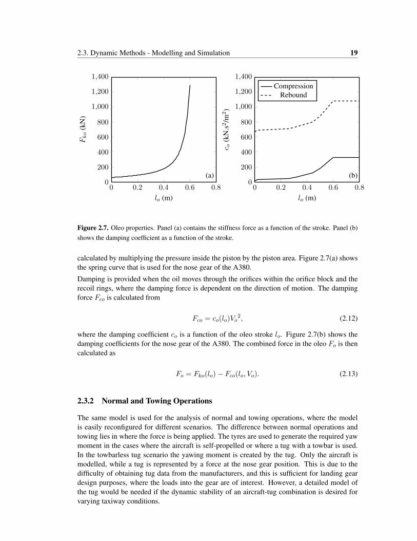
A level attitude is desired when the aircraft is standing on the runway, and therefore the staticload should be calculated for the maximum aircraft weight, at the fore and aft CG positions.The extended stroke lengths are calculated from the aircraft geometric considerations, and thenan initial estimate is made of the stroke that is required, based on previous aircraft. Compres-sion ratios are then chosen based on experience, where a static to extended ratio of 4:1 anda compressed to static ratio of 3:1 are generally used [17]. The spring force Fko can then be
2.3. Dynamic Methods - Modelling and Simulation 19
0 0.2 0.4 0.6 0.80
200
400
600
800
1,000
1,200
1,400
(a)
lo (m)
Fko
(kN
)
0 0.2 0.4 0.6 0.80
200
400
600
800
1,000
1,200
1,400
(b)
lo (m)
c o(k
N.s2/m
2)
CompressionRebound
Figure 2.7. Oleo properties. Panel (a) contains the stiffness force as a function of the stroke. Panel (b)shows the damping coefficient as a function of the stroke.
calculated by multiplying the pressure inside the piston by the piston area. Figure 2.7(a) showsthe spring curve that is used for the nose gear of the A380.
Damping is provided when the oil moves through the orifices within the orifice block and therecoil rings, where the damping force is dependent on the direction of motion. The dampingforce Fco is calculated from
Fco = co(lo)Vo2, (2.12)
where the damping coefficient co is a function of the oleo stroke lo. Figure 2.7(b) shows thedamping coefficients for the nose gear of the A380. The combined force in the oleo Fo is thencalculated as
Fo = Fko(lo)− Fco(lo, Vo). (2.13)
2.3.2 Normal and Towing Operations
The same model is used for the analysis of normal and towing operations, where the modelis easily reconfigured for different scenarios. The difference between normal operations andtowing lies in where the force is being applied. The tyres are used to generate the required yawmoment in the cases where the aircraft is self-propelled or where a tug with a towbar is used.In the towbarless tug scenario the yawing moment is created by the tug. Only the aircraft ismodelled, while a tug is represented by a force at the nose gear position. This is due to thedifficulty of obtaining tug data from the manufacturers, and this is sufficient for landing geardesign purposes, where the loads into the gear are of interest. However, a detailed model ofthe tug would be needed if the dynamic stability of an aircraft-tug combination is desired forvarying taxiway conditions.
20 Chapter 2. Models and Hierarchy of Analysis Methods
20 40 60 80 100 120 140 16020
40
60
80
100
120
at0
x (m)
y(m
)Test Data
Simulation
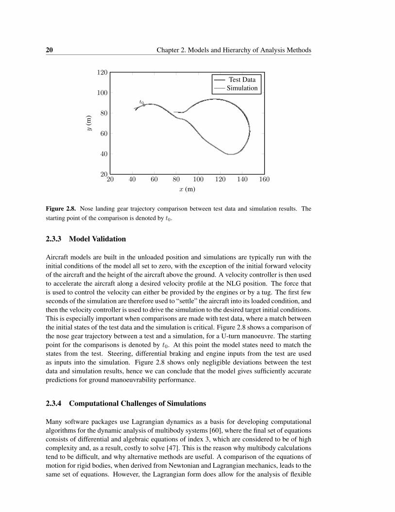
Figure 2.8. Nose landing gear trajectory comparison between test data and simulation results. Thestarting point of the comparison is denoted by t0.
2.3.3 Model Validation
Aircraft models are built in the unloaded position and simulations are typically run with theinitial conditions of the model all set to zero, with the exception of the initial forward velocityof the aircraft and the height of the aircraft above the ground. A velocity controller is then usedto accelerate the aircraft along a desired velocity profile at the NLG position. The force thatis used to control the velocity can either be provided by the engines or by a tug. The first fewseconds of the simulation are therefore used to “settle” the aircraft into its loaded condition, andthen the velocity controller is used to drive the simulation to the desired target initial conditions.This is especially important when comparisons are made with test data, where a match betweenthe initial states of the test data and the simulation is critical. Figure 2.8 shows a comparison ofthe nose gear trajectory between a test and a simulation, for a U-turn manoeuvre. The startingpoint for the comparisons is denoted by t0. At this point the model states need to match thestates from the test. Steering, differential braking and engine inputs from the test are usedas inputs into the simulation. Figure 2.8 shows only negligible deviations between the testdata and simulation results, hence we can conclude that the model gives sufficiently accuratepredictions for ground manoeuvrability performance.
2.3.4 Computational Challenges of Simulations
Many software packages use Lagrangian dynamics as a basis for developing computationalalgorithms for the dynamic analysis of multibody systems [60], where the final set of equationsconsists of differential and algebraic equations of index 3, which are considered to be of highcomplexity and, as a result, costly to solve [47]. This is the reason why multibody calculationstend to be difficult, and why alternative methods are useful. A comparison of the equations ofmotion for rigid bodies, when derived from Newtonian and Lagrangian mechanics, leads to thesame set of equations. However, the Lagrangian form does allow for the analysis of flexible

2.4. Bifurcation Methods 21
bodies, leading to simulations that are even more computationally intensive when structuralmodes are included into the model. A detailed description of the calculations that are involvedin multibody dynamics is not within the scope of this paper; the interested reader can obtainmore details from references [9] and [60].
Design of experiments (DOE), where the design space is divided into a grid of different combi-nations of steering angles and velocities, provides a means to determine the effect of parameterchanges on the dynamics of a system. All the dynamic effects are taken into consideration,and this leads to more reliable predictions. The user is able to test detailed steering and brak-ing control-logic algorithms, balancing the aircraft performance against the loads on the gearand tyres. However, it does not necessarily mean that all the dynamics have been categorised,especially for highly nonlinear systems. A penalty is also incurred due to the difficulty inautomating the testing of such manoeuvres, as well as the high CPU times required for suchsimulations. Simulations are conducted at very specific operating conditions during the conceptphase for trade-off studies. Small parts of the envelope are covered. These initial simulationsare also used in support of bifurcation analysis predictions, where bifurcation methods allowfor complete coverage of the envelope. Extensive simulations are conducted in the later stagesof a major aircraft programme, as, and when, data becomes available.
2.4 Bifurcation Methods
The high cost associated with simulations makes numerical continuation techniques attrac-tive, due to the speed with which a global picture of the dynamics can be constructed. Spe-cific regions of interest can be identified for further detailed analysis with multibody dynamiccodes [13, 15, 54]. Previous studies of the A320 showed how bifurcation methods can be usedto detect stability margins, showing how specific bifurcations can be attributed to the loss ofgrip at specific tyres on the aircraft [13, 54, 55]. The Dynamical Systems Toolbox that wasdeveloped at the University of Bristol allows for the seamless integration of Simulink or Sim-Mechanics models [15].
It is important to note that the simulation models that are discussed earlier are in fact alsoused for the bifurcation analysis. This is a very useful feature, as these models are likely tobe developed in other parts of the company. Hence it is possible to “plug” existing modelsinto the bifurcation analysis framework provided by the toolbox, avoiding the rebuilding ofmodels specifically for the purpose of bifurcation analysis. Another benefit of the toolbox isthe additional information that can be obtained from the models. All the tyre data is available,which allows for the construction of supplementary information that would normally not bereadily available [15]. It is for instance possible to represent the data in new ways that givesone a much better understanding of how the loads are distributed amongst the tyres. Figures 6.9and 6.10 in Section 6.4.3 are a good example of new types of graphs that can be used to depicta global view of the force distribution in the tyres as a result of using numerical continuationtechniques.
2.4.1 Bifurcation Theory
Dynamical systems theory provides a methodology for studying systems of nonlinear ordinarydifferential equations. A key method is that of bifurcation analysis, where one identifies differ-
22 Chapter 2. Models and Hierarchy of Analysis Methods
ent ways in which the dynamics of the system can change. In combination with the numericaltechnique of continuation, one can perform a nonlinear stability analysis by following solutionsand detecting their stability changes (bifurcations). The bifurcations can then be followed inmore parameters to identify regions in parameter space that correspond to different behaviourof the system. See, for example [29] and [62] as entry points to the literature.
To summarise some basic ideas consider an ODE model of the form
u = f(u, λ). (2.14)
where u is an n-dimensional state vector, λ a (multidimensional) control parameter, and f asufficiently smooth (typically nonlinear) function. In terms of standard equations of motionfor an aircraft on the ground, the state vector u contains the aircraft translational and rotationalstates, along with the translational states of the oleos, as described in Section 2.3.1 and Ap-pendix C. The control parameter consists of the steering angle, thrust, the position of the CG,and possibly other relevant parameters. Equilibrium solutions of (2.14), also known as trimconditions, satisfy
f(u0, λ) = 0. (2.15)
The implicit function (2.15) defines a solution locus of equilibria, which is a one-dimensionalsolution curve when a single parameter, such as the steering angle, is varied. The stability of theequilibria can be determined from the (n× n) Jacobian matrix Df of partial derivatives of thefunction f with respect to the state u. Continuation software, such as the package AUTO [19],or the Dynamical Systems Toolbox used here, is able to follow curves of equilibria whilemonitoring their stability. See also [37] for an overview of the different software packages thatare available. Changes of stability, that is, bifurcations, are automatically detected and can thenbe followed in additional parameters. Similarly, periodic solutions can be followed and theirstability changes detected. The continuation of suitable solution curves allows one to build upa comprehensive picture of the overall dynamics in a systematic way.
Typical bifurcations such as saddle-node (fold) and Hopf bifurcations (onset of oscillations)can be found in engineering systems. Previous work on ground manoeuvring has indeed foundoscillatory behaviour at higher velocity and thrust ranges [13, 54, 55]. Bifurcation analysis isnow a standard and powerful tool that is being used extensively in engineering applications, andmore recently for the analysis of landing gears and aircraft ground dynamics [13, 54, 55, 64].
2.4.2 Dynamical Systems Toolbox — AUTO Integration into Matlab
Bifurcation methods have not been readily adopted by the engineering community becausethe methods and tools available have thus far been developed and used mainly within an aca-demic environment. The development of a Dynamical Systems Toolbox within the Matlabenvironment is our attempt to consolidate previous efforts at the University of Bristol to createa user-friendly environment for engineers [16]. Other efforts around the world to develop dy-namical systems software in Matlab exist, such as MATCONT [28], but it appears that this hasnot been widely adopted by the engineering community. We have thus tried to obtain the best
2.4. Bifurcation Methods 23
of both worlds by integrating the existing Fortran AUTO code into Matlab via mex-functions.This allows us to use the speed of a lower level language with the user-friendly interface ofMatlab, along with access to the existing algorithms available in AUTO.
Another important aspect of the toolbox is that engineering tools such as Simulink and SimMe-chanics can be integrated with the dynamical systems software. In this way, industrially testedmodels can be used directly in this environment — without the need for converting models toa format that can be used by the stand-alone version of AUTO. More specifically, AUTO hasdirect access to the states of the Simulink/SimMechanics model.
More widespread use of the Dynamical Systems Toolbox will be promoted by providing doc-umentation and reference material that is easy to use, with concrete examples for the user. Wehave combined most of the user manual of AUTO with our own examples, and integrated thisinto the Matlab help environment. The Dynamical Systems Toolbox therefore feels like anyother toolbox that has been developed for Matlab, where the user can select the toolbox fromthe menu, with the accompanying help and search functionality. We have also started to de-velop components with the new object oriented programming capability in Matlab, which willenhance the pace at which new applications will be developed in the future. Appendix D canbe consulted for more details on how the toolbox was developed and how to obtain the sourcecode.
2.4.3 Application to Ground Manoeuvres
The continuation analysis starts from an equilibrium solution that is obtained from a previousbifurcation run, or from a simulation. The method used here is in fact the latter, where a velocitycontroller is used to control the engine or towing force until a target velocity is reached. Atthis stage the steering angle is set to 0◦, and consequently the aircraft is moving in a straightline. Similar steps to that of the simulation approach are followed up to this point. The velocitycontroller is then switched off so that the engines are operating at a constant thrust.
A continuation run is initiated as soon as the software recognises that an equilibrium conditionhas been reached (zero gradients for the continuation states). Instead of feeding the steering in-put into an ODE solver, the steering input is provided to the Dynamical Systems Toolbox. Thealgorithm then follows these equilibrium states as a parameter (e.g. steering angle) is varied,while their stability is monitored. The occurrence of fold and Hopf bifurcations [37] is moni-tored, and they indicate a change in the dynamics when detected. All the tyre and gear forcesare provided for each equilibrium state, where these forces represent those needed to obtaintrim conditions. This provides an immense amount of freedom in the design process, and al-lows one to follow any solution of interest in the relevant parameters. The user can for instanceset a specific condition (algebraic constraint) on the tyre forces, and then follow this conditiondirectly, without having to do exhaustive simulations, to obtain the envelope for the prescribedcondition. See [13] and [53] for an exact explanation of how the analysis is conducted.
We use continuation algorithms in Chapter 3 to obtain steady-state turn radii as the steeringangle is varied. In Chapter 4 we show how continuation methods can be used to determineif sustained towing manoeuvres will have a beneficial or detrimental effect on the tyres. InChapter 5 we show how the steering angle that is needed for a runway exit can be obtaineddirectly from continuation analysis, instead of using simulations. In Chapter 6 we show that

24 Chapter 2. Models and Hierarchy of Analysis Methods
steady-state conditions can be used to analyse the lateral ground loads for a high-speed turn,making continuation methods the perfect tool for such analysis.
Chapter 3
Low-Speed: U-turn Manoeuvres
3.1 Introduction
The Boeing 747 has long been used as the baseline for specifying requirements to which largeinternational airports must adhere. This means that new civil aircraft designs have to staywithin the manoeuvrability requirements of this aircraft to ensure that no significant investmentis needed for upgrades to existing airport infrastructure. This is also the case for the AirbusA380, for which only terminal facilities need to be upgraded, while runways and taxiways donot require any significant alterations.
The most basic and widely used analysis techniques for early design use purely geometricand static relationships between the gear positions to determine the turn radius of the aircraft.However, it can be shown that the centre of gravity (CG) location, tyre and brake propertiesdo in fact play a significant role in the overall performance, which means that the static gearlayout alone does not determine the possible turn radius. In this chapter we specifically focuson the U-turn manoeuvre, and analyse the way in which this manoeuvre is conducted. Not allthe parameters that define a U-turn manoeuvre are entirely understood due to the demandingnature of this manoeuvre, especially for large aircraft such as the A380.
One important property of the overall aircraft model lies in the nonlinear nature of landing gearcomponents, for example, due to geometric effects or large tyre deflections. Therefore, smallperturbations in velocity, steering angle or brake application may lead to significant differencesin the final turn width. In a previous study we showed that it is possible to calculate the radiusof turn for a specific thrust case as the steering angle is varied [13]. In this chapter a comparisonis made between the most widely used methods for the analysis of U-turn manoeuvres, whichconsist of geometric and simulation approaches, and a new approach where dynamical systemstheory is used to determine the turn width. The advantage of the latter is that it combines thenecessary accuracy with computational efficiency.
It is shown that the feasible region of a U-turn is defined by an algebraic constraint, where thedesired turn width forms a boundary. Bifurcation methods are used to follow this constraintas parameters, such as thrust and steering angle, are varied. From the practical point of view,the size and location of the feasible region give a clear picture of whether or not a groundmanoeuvre can be conducted. The bifurcation diagrams considered in this study encapsulateall the information that a design engineer would need in terms of turn widths, edge-clearance
25
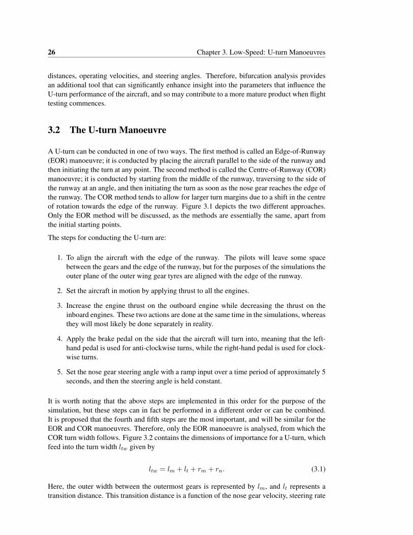
26 Chapter 3. Low-Speed: U-turn Manoeuvres
distances, operating velocities, and steering angles. Therefore, bifurcation analysis providesan additional tool that can significantly enhance insight into the parameters that influence theU-turn performance of the aircraft, and so may contribute to a more mature product when flighttesting commences.
3.2 The U-turn Manoeuvre
A U-turn can be conducted in one of two ways. The first method is called an Edge-of-Runway(EOR) manoeuvre; it is conducted by placing the aircraft parallel to the side of the runway andthen initiating the turn at any point. The second method is called the Centre-of-Runway (COR)manoeuvre; it is conducted by starting from the middle of the runway, traversing to the side ofthe runway at an angle, and then initiating the turn as soon as the nose gear reaches the edge ofthe runway. The COR method tends to allow for larger turn margins due to a shift in the centreof rotation towards the edge of the runway. Figure 3.1 depicts the two different approaches.Only the EOR method will be discussed, as the methods are essentially the same, apart fromthe initial starting points.
The steps for conducting the U-turn are:
1. To align the aircraft with the edge of the runway. The pilots will leave some spacebetween the gears and the edge of the runway, but for the purposes of the simulations theouter plane of the outer wing gear tyres are aligned with the edge of the runway.
2. Set the aircraft in motion by applying thrust to all the engines.
3. Increase the engine thrust on the outboard engine while decreasing the thrust on theinboard engines. These two actions are done at the same time in the simulations, whereasthey will most likely be done separately in reality.
4. Apply the brake pedal on the side that the aircraft will turn into, meaning that the left-hand pedal is used for anti-clockwise turns, while the right-hand pedal is used for clock-wise turns.
5. Set the nose gear steering angle with a ramp input over a time period of approximately 5seconds, and then the steering angle is held constant.
It is worth noting that the above steps are implemented in this order for the purpose of thesimulation, but these steps can in fact be performed in a different order or can be combined.It is proposed that the fourth and fifth steps are the most important, and will be similar for theEOR and COR manoeuvres. Therefore, only the EOR manoeuvre is analysed, from which theCOR turn width follows. Figure 3.2 contains the dimensions of importance for a U-turn, whichfeed into the turn width ltw given by
ltw = lm + lt + rm + rn. (3.1)
Here, the outer width between the outermost gears is represented by lm, and lt represents atransition distance. This transition distance is a function of the nose gear velocity, steering rate
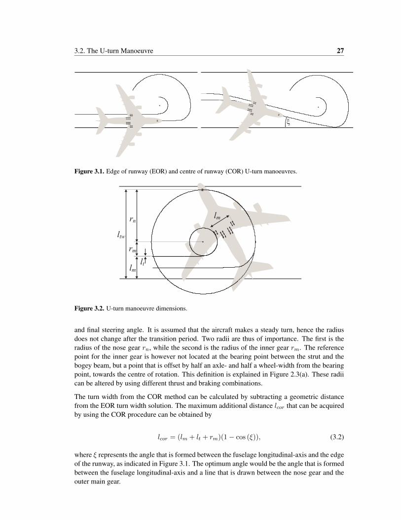
3.2. The U-turn Manoeuvre 27
x
Figure 3.1. Edge of runway (EOR) and centre of runway (COR) U-turn manoeuvres.
lt
lm
rm
rn
ltw
lm
Figure 3.2. U-turn manoeuvre dimensions.
and final steering angle. It is assumed that the aircraft makes a steady turn, hence the radiusdoes not change after the transition period. Two radii are thus of importance. The first is theradius of the nose gear rn, while the second is the radius of the inner gear rm. The referencepoint for the inner gear is however not located at the bearing point between the strut and thebogey beam, but a point that is offset by half an axle- and half a wheel-width from the bearingpoint, towards the centre of rotation. This definition is explained in Figure 2.3(a). These radiican be altered by using different thrust and braking combinations.
The turn width from the COR method can be calculated by subtracting a geometric distancefrom the EOR turn width solution. The maximum additional distance lcor that can be acquiredby using the COR procedure can be obtained by
lcor = (lm + lt + rm)(1− cos (ξ)), (3.2)
where ξ represents the angle that is formed between the fuselage longitudinal-axis and the edgeof the runway, as indicated in Figure 3.1. The optimum angle would be the angle that is formedbetween the fuselage longitudinal-axis and a line that is drawn between the nose gear and theouter main gear.
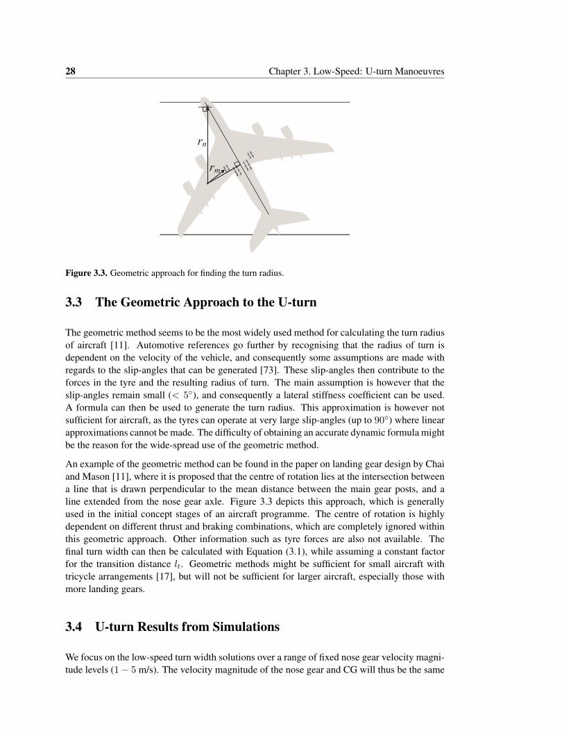
28 Chapter 3. Low-Speed: U-turn Manoeuvres
rn
rm
Figure 3.3. Geometric approach for finding the turn radius.
3.3 The Geometric Approach to the U-turn
The geometric method seems to be the most widely used method for calculating the turn radiusof aircraft [11]. Automotive references go further by recognising that the radius of turn isdependent on the velocity of the vehicle, and consequently some assumptions are made withregards to the slip-angles that can be generated [73]. These slip-angles then contribute to theforces in the tyre and the resulting radius of turn. The main assumption is however that theslip-angles remain small (< 5◦), and consequently a lateral stiffness coefficient can be used.A formula can then be used to generate the turn radius. This approximation is however notsufficient for aircraft, as the tyres can operate at very large slip-angles (up to 90◦) where linearapproximations cannot be made. The difficulty of obtaining an accurate dynamic formula mightbe the reason for the wide-spread use of the geometric method.
An example of the geometric method can be found in the paper on landing gear design by Chaiand Mason [11], where it is proposed that the centre of rotation lies at the intersection betweena line that is drawn perpendicular to the mean distance between the main gear posts, and aline extended from the nose gear axle. Figure 3.3 depicts this approach, which is generallyused in the initial concept stages of an aircraft programme. The centre of rotation is highlydependent on different thrust and braking combinations, which are completely ignored withinthis geometric approach. Other information such as tyre forces are also not available. Thefinal turn width can then be calculated with Equation (3.1), while assuming a constant factorfor the transition distance lt. Geometric methods might be sufficient for small aircraft withtricycle arrangements [17], but will not be sufficient for larger aircraft, especially those withmore landing gears.
3.4 U-turn Results from Simulations
We focus on the low-speed turn width solutions over a range of fixed nose gear velocity magni-tude levels (1− 5 m/s). The velocity magnitude of the nose gear and CG will thus be the same
3.4. U-turn Results from Simulations 29
when no steering input is given. In contrast, the CG velocity will drop as the steering angle isincreased, while the nose gear velocity is being maintained. Asymmetric thrust configurationsare of most interest, seeing that such configurations provide the smallest possible turn radii. Aproportional-integral thrust controller is used on the outboard engine to ensure that the nosegear velocity is maintained, while the other engines are set to idle-thrust.
In reality the pilot will not set an exact fixed velocity, but this is assumed for automation andcomparison purposes. The gains of the controller are set in such a way as to represent themanner in which the pilot would operate the engine. The nose gear velocity will drop as theaircraft enters the turn, after which the pilot will increase the thrust to maintain the velocity.This thrust increase usually leads to an overshoot of the desired velocity. The pilot corrects theovershoot by decreasing the thrust. The rest of the steps with regards to how the manoeuvresare conducted are as explained in Section 3.2.
A range of steering angles (20◦ − 80◦) and nose gear velocities (1 − 5 m/s) were used for amedium weight A380 configuration. The selection of test points is a balance between capturingthe most important phenomena and simulation run-times. The steering angle was increased by5◦ increments, and the velocity by 0.2 m/s. The simulation run-time for this example wasapproximately 2.5 hours on an Intel 1.8 GHz processor. Greater fidelity can be obtained byusing more test points, but this would be at a significant cost to the run-times. The nonlinearnature of tyres does however mean that areas of rapid transition may occur between certainvelocities and steering angles, and consequently the mesh would need to be refined in theseareas.
The results for the turn width simulations in SimMechanics are shown in Figure 3.4(a), wherethe maximum steering angle (δ) during the simulation is represented on the x-axis, and thenose gear velocity magnitude (Vn) at entry into the turn is represented on the y-axis. Theresulting turn width, or any quantity of interest, is therefore a result of two independent inputs(δ and Vn), and can be represented readily by a contour plot. The area to the right of the 51m contour line indicates the feasible operating region for a U-turn. This value is obtained bysubtracting the required clearance distance (2×4.5) from the 60 m runway width for a CategoryVI airport; the type of airport where an A380 can conduct a U-turn manoeuvre. The turn widthincreases slightly with an increase in velocity at a specific steering angle, but the simulationsseem to indicate that the turn width is not greatly influenced by the velocity for this specificcase. Figure 3.4(b) contains a contour plot of the turn radius of the nose gear as a function ofdifferent steering angles and nose gear velocities.
The transition distance is shown in Figure 3.4(c) and is highly dependent on the actions of thepilot. Reaction times were obtained from flight test data, indicating that the steering input tookplace over the course of 5 seconds. The biggest transition distance occurs at a steering angle of70◦ and a velocity of 4 m/s, and could indicate an area where a transition of loads between tyrestakes place. This would have to be verified by studying the tyre forces from the simulations.
Section 3.2 shows that an additional turn margin can be obtained by using the COR insteadof the EOR method. It can be computed by using Equation (3.2), and this distance is shownin Figure 3.4(d). If it is assumed that the 60 m contour line in Figure 3.4(a) indicates theboundary of the feasible region, then Figure 3.4(d) indicates that an additional margin of up toapproximately 1.0 m can be obtained by using the COR method.
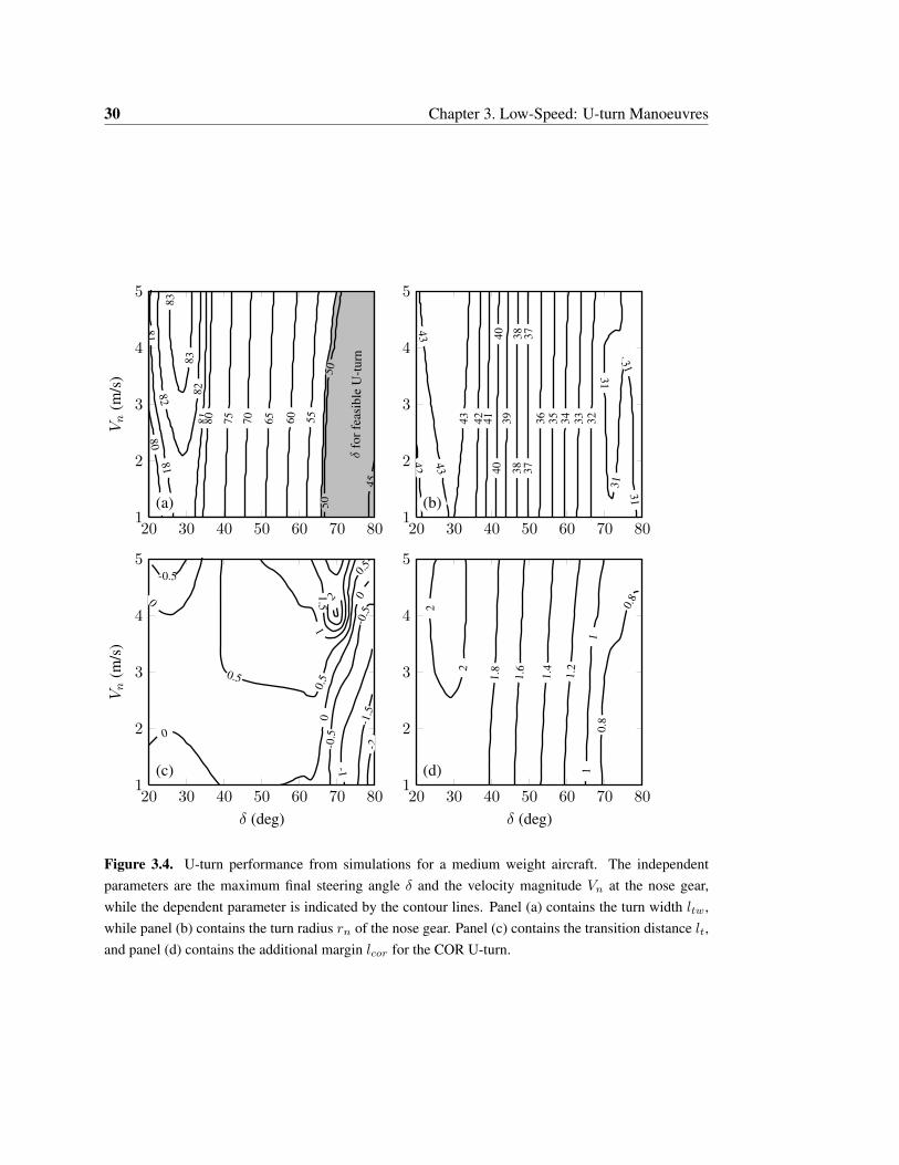
30 Chapter 3. Low-Speed: U-turn Manoeuvres
20 30 40 50 60 70 801
2
3
4
5
5050
83
838282
81
8181
80
80
75 70 65 60 55
45δ
for f
easi
ble
U-t
urn
(a)
Vn
(m/s
)
20 30 40 50 60 70 801
2
3
4
5
4343
4342
4241
4040
3938
3837
3736 35 34 33 32
3131
31
31
(b)
20 30 40 50 60 70 801
2
3
4
5
21.51
0.5
0.50.5
0
0
0
0
-0.5
-0.5
-0.5
-1
-1.5
-2
-2
(c)
δ (deg)
Vn
(m/s
)
20 30 40 50 60 70 801
2
3
4
5
2
2
1.8
1.6
1.6
1.4
1.2
11
0.8
0.8
(d)
δ (deg)
Figure 3.4. U-turn performance from simulations for a medium weight aircraft. The independentparameters are the maximum final steering angle δ and the velocity magnitude Vn at the nose gear,while the dependent parameter is indicated by the contour lines. Panel (a) contains the turn width ltw,while panel (b) contains the turn radius rn of the nose gear. Panel (c) contains the transition distance lt,and panel (d) contains the additional margin lcor for the COR U-turn.
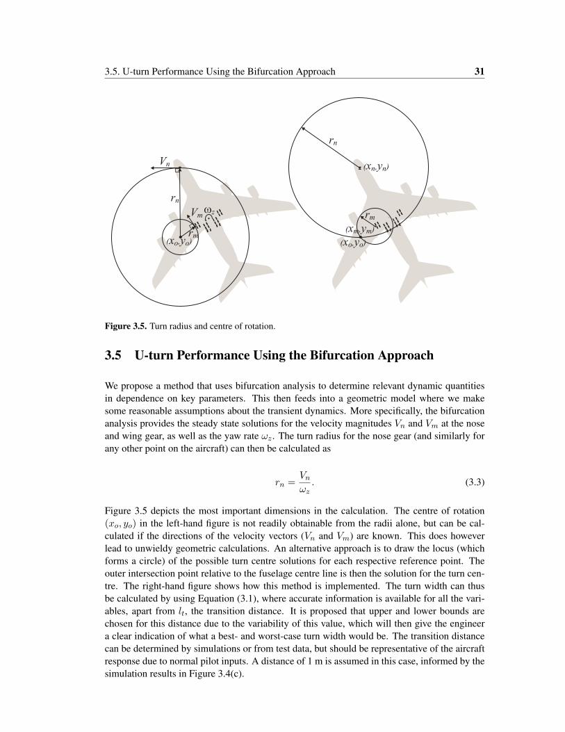
3.5. U-turn Performance Using the Bifurcation Approach 31
rm
rn
rm
rn
Vn
Vm
( , )x yn n
( , )x ym m
( , )x yo o( , )x yo o
wz
Figure 3.5. Turn radius and centre of rotation.
3.5 U-turn Performance Using the Bifurcation Approach
We propose a method that uses bifurcation analysis to determine relevant dynamic quantitiesin dependence on key parameters. This then feeds into a geometric model where we makesome reasonable assumptions about the transient dynamics. More specifically, the bifurcationanalysis provides the steady state solutions for the velocity magnitudes Vn and Vm at the noseand wing gear, as well as the yaw rate ωz . The turn radius for the nose gear (and similarly forany other point on the aircraft) can then be calculated as
rn =Vnωz. (3.3)
Figure 3.5 depicts the most important dimensions in the calculation. The centre of rotation(xo, yo) in the left-hand figure is not readily obtainable from the radii alone, but can be cal-culated if the directions of the velocity vectors (Vn and Vm) are known. This does howeverlead to unwieldy geometric calculations. An alternative approach is to draw the locus (whichforms a circle) of the possible turn centre solutions for each respective reference point. Theouter intersection point relative to the fuselage centre line is then the solution for the turn cen-tre. The right-hand figure shows how this method is implemented. The turn width can thusbe calculated by using Equation (3.1), where accurate information is available for all the vari-ables, apart from lt, the transition distance. It is proposed that upper and lower bounds arechosen for this distance due to the variability of this value, which will then give the engineera clear indication of what a best- and worst-case turn width would be. The transition distancecan be determined by simulations or from test data, but should be representative of the aircraftresponse due to normal pilot inputs. A distance of 1 m is assumed in this case, informed by thesimulation results in Figure 3.4(c).
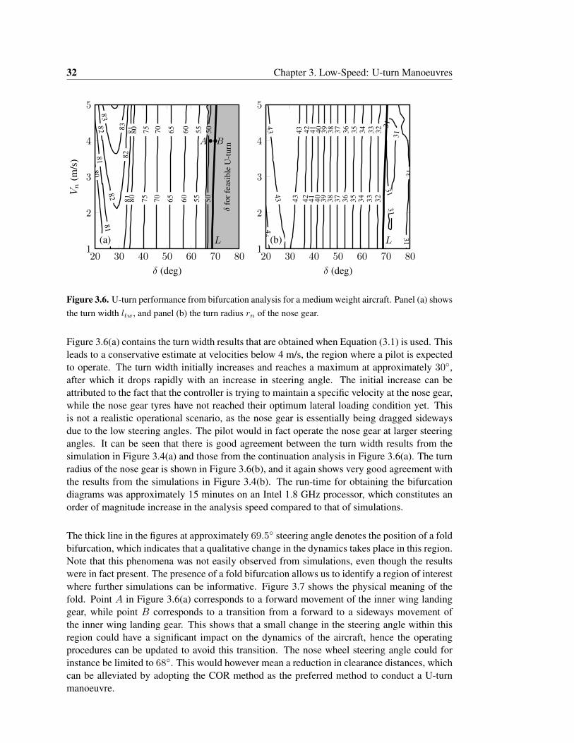
32 Chapter 3. Low-Speed: U-turn Manoeuvres
20 30 40 50 60 70 801
2
3
4
5
83
838282
8281
81
8181
8080
8080
7575
7070
6565
6060
5555
5050
(a) L
δfo
r fea
sibl
eU
-tur
nA B
δ (deg)
Vn
(m/s
)
20 30 40 50 60 70 801
2
3
4
5
4343
4343
4242
4241
4140
4039
3938
3837
3736
3635
3534
3433
3332
32
31
31
31
31
31
31(b) L
δ (deg)
Figure 3.6. U-turn performance from bifurcation analysis for a medium weight aircraft. Panel (a) showsthe turn width ltw, and panel (b) the turn radius rn of the nose gear.
Figure 3.6(a) contains the turn width results that are obtained when Equation (3.1) is used. Thisleads to a conservative estimate at velocities below 4 m/s, the region where a pilot is expectedto operate. The turn width initially increases and reaches a maximum at approximately 30◦,after which it drops rapidly with an increase in steering angle. The initial increase can beattributed to the fact that the controller is trying to maintain a specific velocity at the nose gear,while the nose gear tyres have not reached their optimum lateral loading condition yet. Thisis not a realistic operational scenario, as the nose gear is essentially being dragged sidewaysdue to the low steering angles. The pilot would in fact operate the nose gear at larger steeringangles. It can be seen that there is good agreement between the turn width results from thesimulation in Figure 3.4(a) and those from the continuation analysis in Figure 3.6(a). The turnradius of the nose gear is shown in Figure 3.6(b), and it again shows very good agreement withthe results from the simulations in Figure 3.4(b). The run-time for obtaining the bifurcationdiagrams was approximately 15 minutes on an Intel 1.8 GHz processor, which constitutes anorder of magnitude increase in the analysis speed compared to that of simulations.
The thick line in the figures at approximately 69.5◦ steering angle denotes the position of a foldbifurcation, which indicates that a qualitative change in the dynamics takes place in this region.Note that this phenomena was not easily observed from simulations, even though the resultswere in fact present. The presence of a fold bifurcation allows us to identify a region of interestwhere further simulations can be informative. Figure 3.7 shows the physical meaning of thefold. Point A in Figure 3.6(a) corresponds to a forward movement of the inner wing landinggear, while point B corresponds to a transition from a forward to a sideways movement ofthe inner wing landing gear. This shows that a small change in the steering angle within thisregion could have a significant impact on the dynamics of the aircraft, hence the operatingprocedures can be updated to avoid this transition. The nose wheel steering angle could forinstance be limited to 68◦. This would however mean a reduction in clearance distances, whichcan be alleviated by adopting the COR method as the preferred method to conduct a U-turnmanoeuvre.
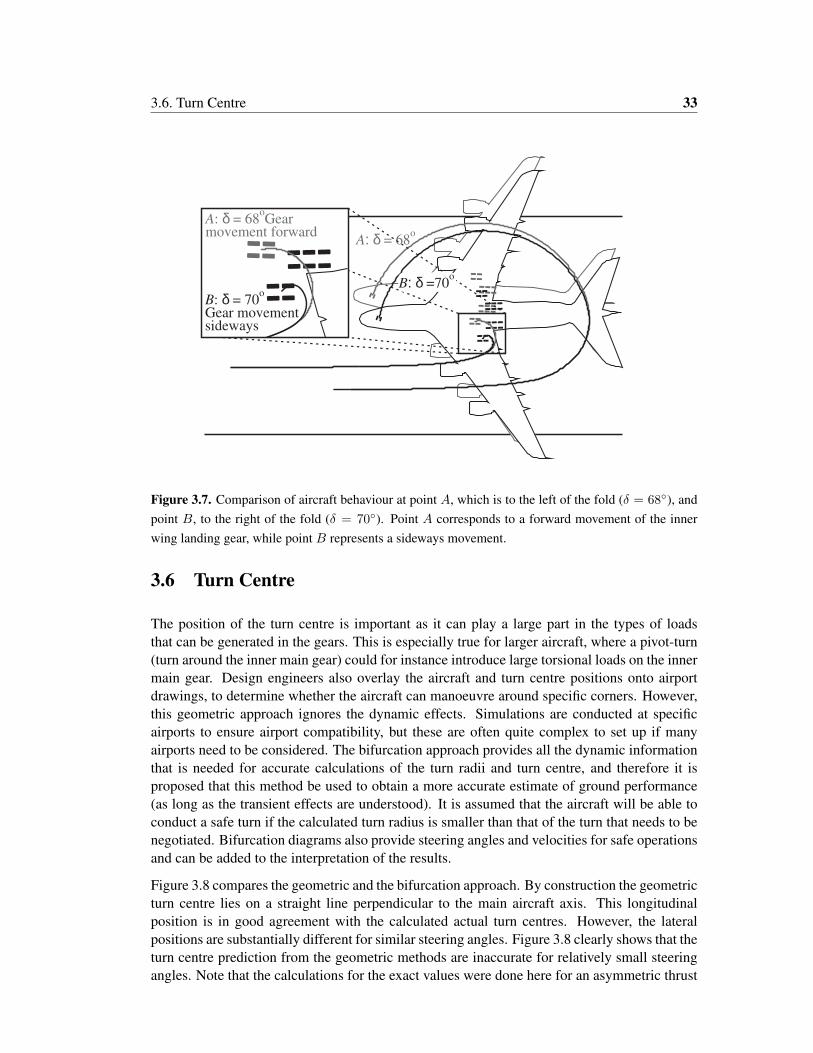
3.6. Turn Centre 33
B:Gear movementsideways
δ = 70o
A: Gearmovement forward
δ = 68o
A: δ = 68o
B: δ =70o
Figure 3.7. Comparison of aircraft behaviour at point A, which is to the left of the fold (δ = 68◦), andpoint B, to the right of the fold (δ = 70◦). Point A corresponds to a forward movement of the innerwing landing gear, while point B represents a sideways movement.
3.6 Turn Centre
The position of the turn centre is important as it can play a large part in the types of loadsthat can be generated in the gears. This is especially true for larger aircraft, where a pivot-turn(turn around the inner main gear) could for instance introduce large torsional loads on the innermain gear. Design engineers also overlay the aircraft and turn centre positions onto airportdrawings, to determine whether the aircraft can manoeuvre around specific corners. However,this geometric approach ignores the dynamic effects. Simulations are conducted at specificairports to ensure airport compatibility, but these are often quite complex to set up if manyairports need to be considered. The bifurcation approach provides all the dynamic informationthat is needed for accurate calculations of the turn radii and turn centre, and therefore it isproposed that this method be used to obtain a more accurate estimate of ground performance(as long as the transient effects are understood). It is assumed that the aircraft will be able toconduct a safe turn if the calculated turn radius is smaller than that of the turn that needs to benegotiated. Bifurcation diagrams also provide steering angles and velocities for safe operationsand can be added to the interpretation of the results.
Figure 3.8 compares the geometric and the bifurcation approach. By construction the geometricturn centre lies on a straight line perpendicular to the main aircraft axis. This longitudinalposition is in good agreement with the calculated actual turn centres. However, the lateralpositions are substantially different for similar steering angles. Figure 3.8 clearly shows that theturn centre prediction from the geometric methods are inaccurate for relatively small steeringangles. Note that the calculations for the exact values were done here for an asymmetric thrust
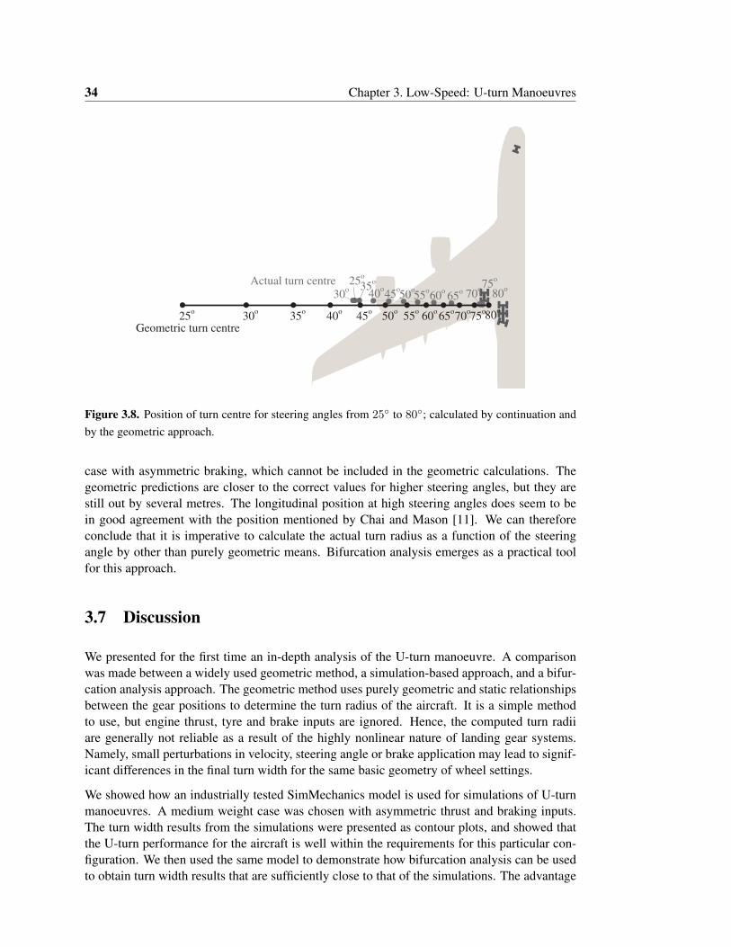
34 Chapter 3. Low-Speed: U-turn Manoeuvres
25o
30o 35
o
40o45
o50
o
55o60
o65
o 70o75
o
80o
30o
35o
40o
45o
50o
55o
60o65
o70
o75
o80
o
25o
Actual turn centre
Geometric turn centre
Figure 3.8. Position of turn centre for steering angles from 25◦ to 80◦; calculated by continuation andby the geometric approach.
case with asymmetric braking, which cannot be included in the geometric calculations. Thegeometric predictions are closer to the correct values for higher steering angles, but they arestill out by several metres. The longitudinal position at high steering angles does seem to bein good agreement with the position mentioned by Chai and Mason [11]. We can thereforeconclude that it is imperative to calculate the actual turn radius as a function of the steeringangle by other than purely geometric means. Bifurcation analysis emerges as a practical toolfor this approach.
3.7 Discussion
We presented for the first time an in-depth analysis of the U-turn manoeuvre. A comparisonwas made between a widely used geometric method, a simulation-based approach, and a bifur-cation analysis approach. The geometric method uses purely geometric and static relationshipsbetween the gear positions to determine the turn radius of the aircraft. It is a simple methodto use, but engine thrust, tyre and brake inputs are ignored. Hence, the computed turn radiiare generally not reliable as a result of the highly nonlinear nature of landing gear systems.Namely, small perturbations in velocity, steering angle or brake application may lead to signif-icant differences in the final turn width for the same basic geometry of wheel settings.
We showed how an industrially tested SimMechanics model is used for simulations of U-turnmanoeuvres. A medium weight case was chosen with asymmetric thrust and braking inputs.The turn width results from the simulations were presented as contour plots, and showed thatthe U-turn performance for the aircraft is well within the requirements for this particular con-figuration. We then used the same model to demonstrate how bifurcation analysis can be usedto obtain turn width results that are sufficiently close to that of the simulations. The advantage
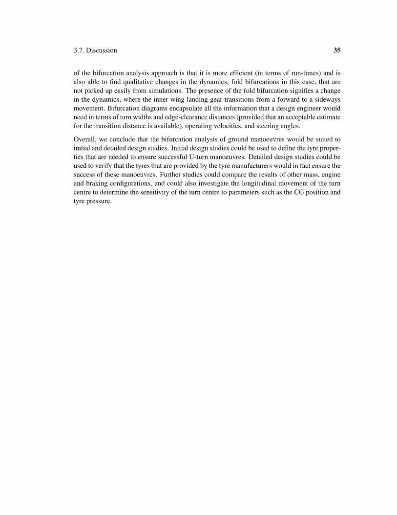
3.7. Discussion 35
of the bifurcation analysis approach is that it is more efficient (in terms of run-times) and isalso able to find qualitative changes in the dynamics, fold bifurcations in this case, that arenot picked up easily from simulations. The presence of the fold bifurcation signifies a changein the dynamics, where the inner wing landing gear transitions from a forward to a sidewaysmovement. Bifurcation diagrams encapsulate all the information that a design engineer wouldneed in terms of turn widths and edge-clearance distances (provided that an acceptable estimatefor the transition distance is available), operating velocities, and steering angles.
Overall, we conclude that the bifurcation analysis of ground manoeuvres would be suited toinitial and detailed design studies. Initial design studies could be used to define the tyre proper-ties that are needed to ensure successful U-turn manoeuvres. Detailed design studies could beused to verify that the tyres that are provided by the tyre manufacturers would in fact ensure thesuccess of these manoeuvres. Further studies could compare the results of other mass, engineand braking configurations, and could also investigate the longitudinal movement of the turncentre to determine the sensitivity of the turn centre to parameters such as the CG position andtyre pressure.

Chapter 4
Low- and Medium-Speed: Towing
4.1 Introduction
Aircraft ground operations comprise of a combination of tug and self-propelled movements.Tug operations tend to consist of pushbacks from the gate until the aircraft reaches a favourableorientation for movement under its own power, or maintenance towing between the hangarsand the gates. Taxi operations, on the other-hand, are presently conducted with the aid ofthe aircraft’s engines. One only has to venture to the nearest airport to notice that aircraftoften stand around for extended periods while waiting for take-off clearance, which leads tounnecessary fuel consumption. Ideas related to the towing of aircraft to a starting grid close tothe runway threshold have been mentioned for the purposes of fuel savings [5]. Recent mediareports state that the use of tugs during taxiing will allow pilots to keep the engines turnedoff until the aircraft reaches the runway, where the tug is then separated from the aircraft [5].The opposite is also true after the aircraft has landed. From the literature available on remote-controlled tugs, it appears that the pilot would control the tug from the cockpit [5], and thata tug driver would manoeuvre the tug around the gate, meaning that no extra manpower willbe needed. Another advantage is that no physical modifications to the aircraft are necessary.A less obvious advantage relates to the turn around time at the gate, which is often prescribedby a threshold temperature of the brakes: the aircraft is not allowed to dispatch if the braketemperature is above a certain value. A system that could minimise the use of the aircraftbrakes would therefore not only reduce the energy that is absorbed into the brakes, but willalso reduce brake and tyre wear and allow for shorter intervals at the gate.
This chapter addresses the issue of aircraft towing stability in Section 4.2, by building onprevious work related to the towing of truck-trailer combinations [25]; this also forms thestarting point for many other studies related to the control of towed vehicles [6, 61, 72]. Thefocus in these papers was on straight-line and circular towing stability, which is also directlyapplicable to a tug that is towing an aircraft. Airport apron and taxiway markings consist ofa combination of straight and circumferential lines, hence the analyses of straight and circularmanoeuvres are adequate. In this study we focus on towbarless tugs with a typical arrangementdepicted in Figure 4.1. The wheels are clamped in a cradle within the tug, and consequently therelative motion between the aircraft and tug is around the rotation axis of the nose gear strut.It is not clear if towbarless tugs are the preferred option for moving aircraft around airports,compared to tugs with towbars, but towbarless tugs do have several distinct advantages:
37
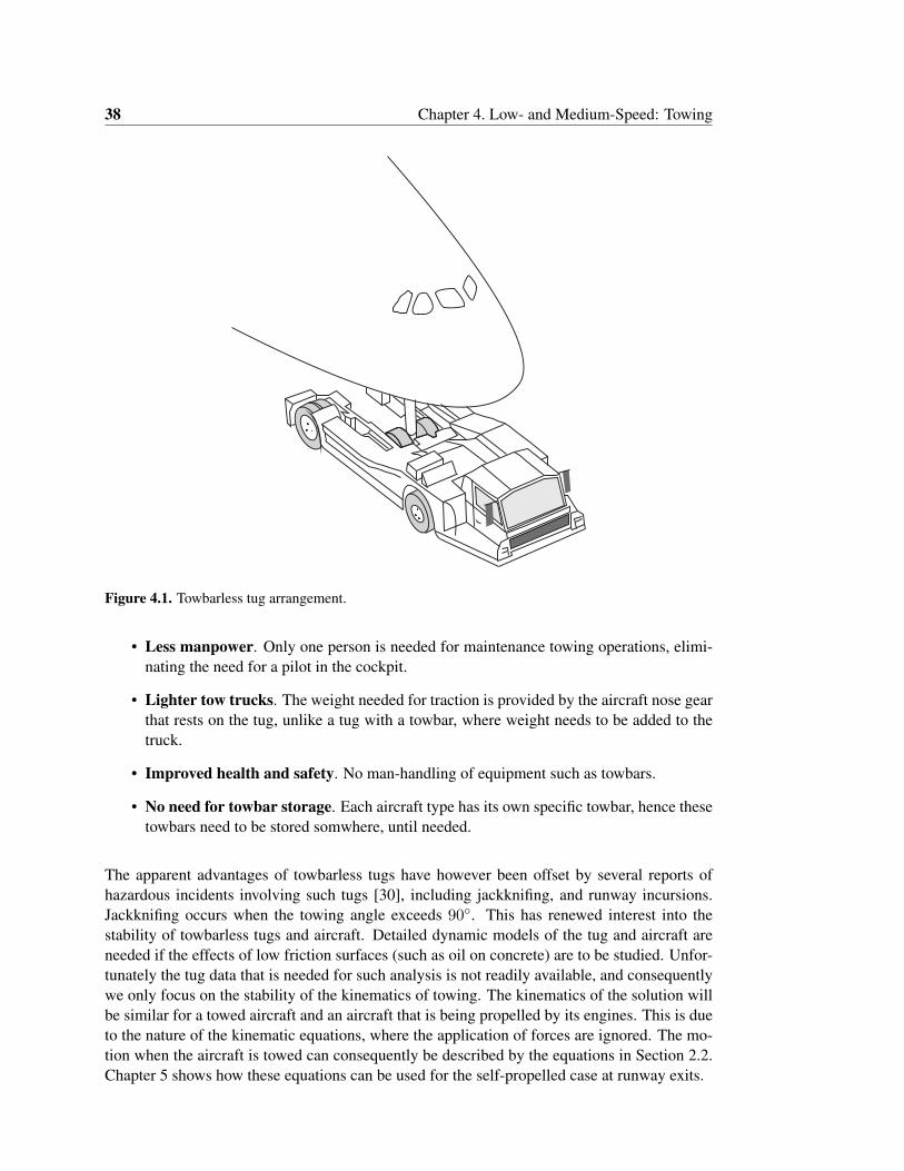
38 Chapter 4. Low- and Medium-Speed: Towing
Figure 4.1. Towbarless tug arrangement.
• Less manpower. Only one person is needed for maintenance towing operations, elimi-nating the need for a pilot in the cockpit.
• Lighter tow trucks. The weight needed for traction is provided by the aircraft nose gearthat rests on the tug, unlike a tug with a towbar, where weight needs to be added to thetruck.
• Improved health and safety. No man-handling of equipment such as towbars.
• No need for towbar storage. Each aircraft type has its own specific towbar, hence thesetowbars need to be stored somwhere, until needed.
The apparent advantages of towbarless tugs have however been offset by several reports ofhazardous incidents involving such tugs [30], including jackknifing, and runway incursions.Jackknifing occurs when the towing angle exceeds 90◦. This has renewed interest into thestability of towbarless tugs and aircraft. Detailed dynamic models of the tug and aircraft areneeded if the effects of low friction surfaces (such as oil on concrete) are to be studied. Unfor-tunately the tug data that is needed for such analysis is not readily available, and consequentlywe only focus on the stability of the kinematics of towing. The kinematics of the solution willbe similar for a towed aircraft and an aircraft that is being propelled by its engines. This is dueto the nature of the kinematic equations, where the application of forces are ignored. The mo-tion when the aircraft is towed can consequently be described by the equations in Section 2.2.Chapter 5 shows how these equations can be used for the self-propelled case at runway exits.
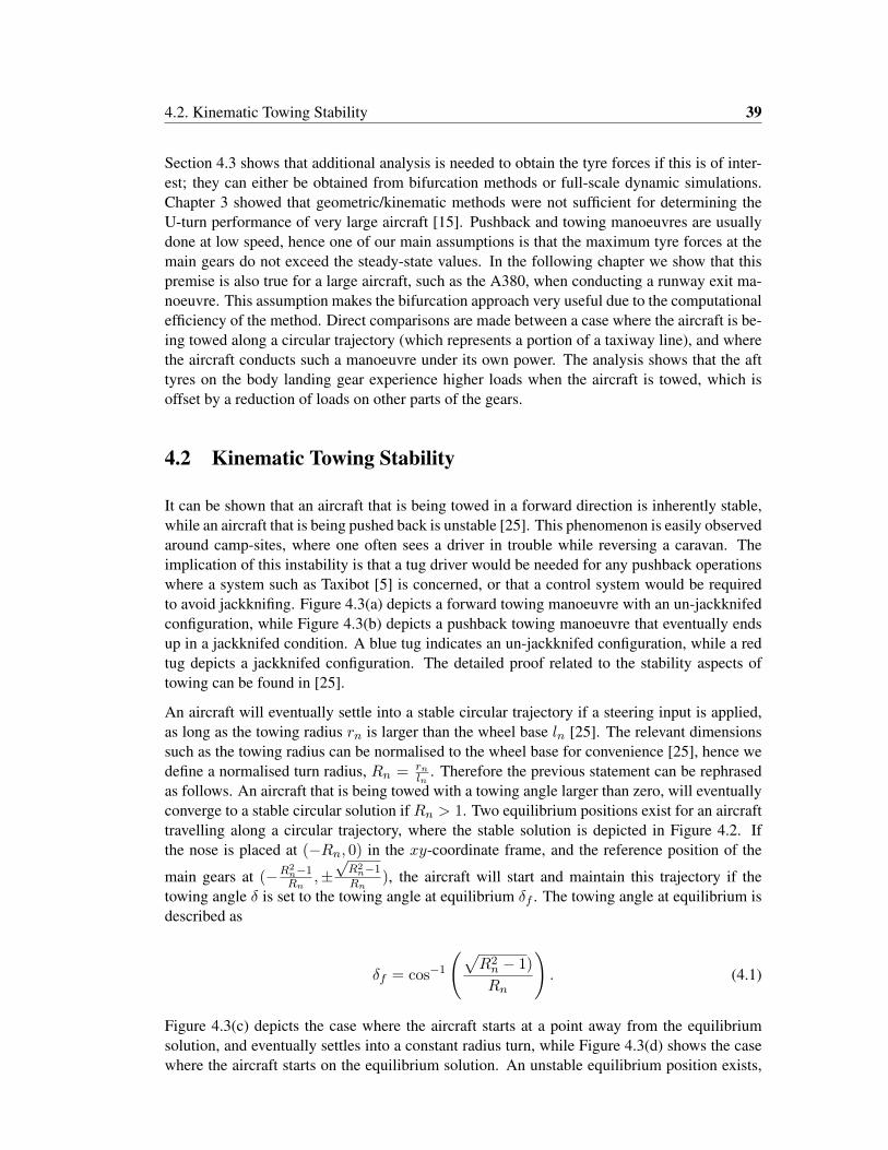
4.2. Kinematic Towing Stability 39
Section 4.3 shows that additional analysis is needed to obtain the tyre forces if this is of inter-est; they can either be obtained from bifurcation methods or full-scale dynamic simulations.Chapter 3 showed that geometric/kinematic methods were not sufficient for determining theU-turn performance of very large aircraft [15]. Pushback and towing manoeuvres are usuallydone at low speed, hence one of our main assumptions is that the maximum tyre forces at themain gears do not exceed the steady-state values. In the following chapter we show that thispremise is also true for a large aircraft, such as the A380, when conducting a runway exit ma-noeuvre. This assumption makes the bifurcation approach very useful due to the computationalefficiency of the method. Direct comparisons are made between a case where the aircraft is be-ing towed along a circular trajectory (which represents a portion of a taxiway line), and wherethe aircraft conducts such a manoeuvre under its own power. The analysis shows that the afttyres on the body landing gear experience higher loads when the aircraft is towed, which isoffset by a reduction of loads on other parts of the gears.
4.2 Kinematic Towing Stability
It can be shown that an aircraft that is being towed in a forward direction is inherently stable,while an aircraft that is being pushed back is unstable [25]. This phenomenon is easily observedaround camp-sites, where one often sees a driver in trouble while reversing a caravan. Theimplication of this instability is that a tug driver would be needed for any pushback operationswhere a system such as Taxibot [5] is concerned, or that a control system would be requiredto avoid jackknifing. Figure 4.3(a) depicts a forward towing manoeuvre with an un-jackknifedconfiguration, while Figure 4.3(b) depicts a pushback towing manoeuvre that eventually endsup in a jackknifed condition. A blue tug indicates an un-jackknifed configuration, while a redtug depicts a jackknifed configuration. The detailed proof related to the stability aspects oftowing can be found in [25].
An aircraft will eventually settle into a stable circular trajectory if a steering input is applied,as long as the towing radius rn is larger than the wheel base ln [25]. The relevant dimensionssuch as the towing radius can be normalised to the wheel base for convenience [25], hence wedefine a normalised turn radius, Rn = rn
ln. Therefore the previous statement can be rephrased
as follows. An aircraft that is being towed with a towing angle larger than zero, will eventuallyconverge to a stable circular solution if Rn > 1. Two equilibrium positions exist for an aircrafttravelling along a circular trajectory, where the stable solution is depicted in Figure 4.2. Ifthe nose is placed at (−Rn, 0) in the xy-coordinate frame, and the reference position of the
main gears at (−R2n−1Rn
,±√R2
n−1
Rn), the aircraft will start and maintain this trajectory if the
towing angle δ is set to the towing angle at equilibrium δf . The towing angle at equilibrium isdescribed as
δf = cos−1
(√R2n − 1)
Rn
). (4.1)
Figure 4.3(c) depicts the case where the aircraft starts at a point away from the equilibriumsolution, and eventually settles into a constant radius turn, while Figure 4.3(d) shows the casewhere the aircraft starts on the equilibrium solution. An unstable equilibrium position exists,
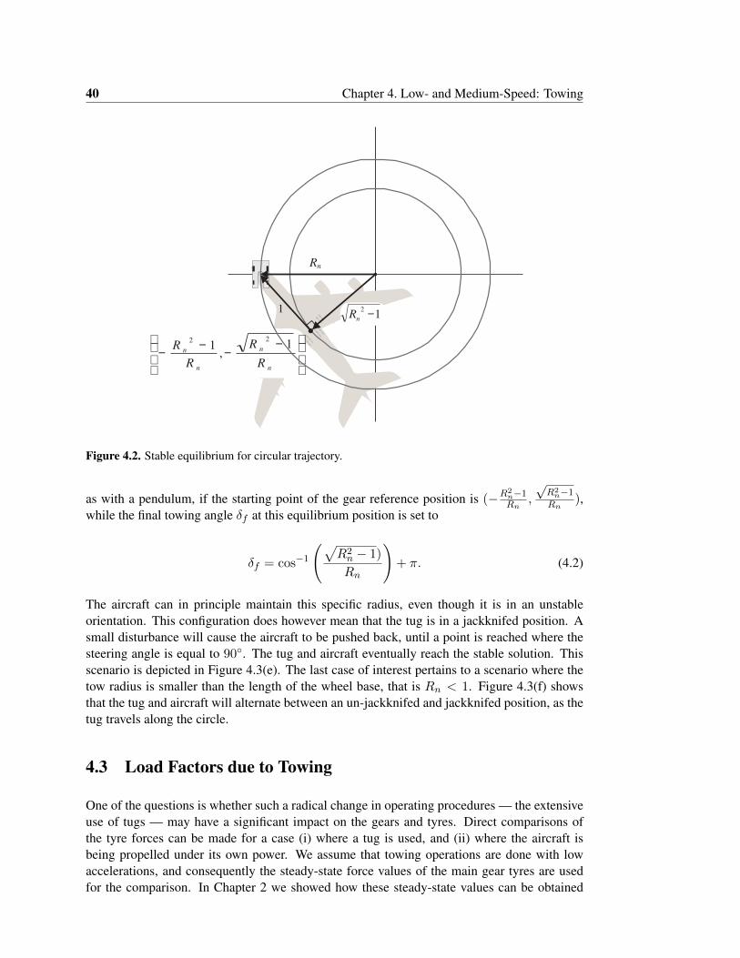
40 Chapter 4. Low- and Medium-Speed: Towing
Rn
11
2 −n
R
−−−−
n
n
n
n
R
R
R
R 1,
122
Figure 4.2. Stable equilibrium for circular trajectory.
as with a pendulum, if the starting point of the gear reference position is (−R2n−1Rn
,
√R2
n−1
Rn),
while the final towing angle δf at this equilibrium position is set to
δf = cos−1
(√R2n − 1)
Rn
)+ π. (4.2)
The aircraft can in principle maintain this specific radius, even though it is in an unstableorientation. This configuration does however mean that the tug is in a jackknifed position. Asmall disturbance will cause the aircraft to be pushed back, until a point is reached where thesteering angle is equal to 90◦. The tug and aircraft eventually reach the stable solution. Thisscenario is depicted in Figure 4.3(e). The last case of interest pertains to a scenario where thetow radius is smaller than the length of the wheel base, that is Rn < 1. Figure 4.3(f) showsthat the tug and aircraft will alternate between an un-jackknifed and jackknifed position, as thetug travels along the circle.
4.3 Load Factors due to Towing
One of the questions is whether such a radical change in operating procedures — the extensiveuse of tugs — may have a significant impact on the gears and tyres. Direct comparisons ofthe tyre forces can be made for a case (i) where a tug is used, and (ii) where the aircraft isbeing propelled under its own power. We assume that towing operations are done with lowaccelerations, and consequently the steady-state force values of the main gear tyres are usedfor the comparison. In Chapter 2 we showed how these steady-state values can be obtained
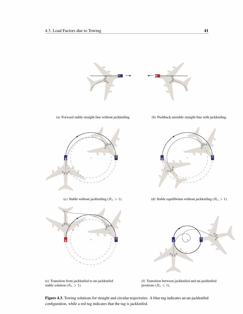
4.3. Load Factors due to Towing 41
(a) Forward stable straight-line without jackknifing (b) Pushback unstable straight-line with jackknifing.
(c) Stable without jackknifing (Rn > 1). (d) Stable equilibrium without jackknifing (Rn > 1).
(e) Transition from jackknifed to un-jackknifedstable solution (Rn > 1).
(f) Transition between jackknifed and un-jackknifedpositions (Rn < 1).
Figure 4.3. Towing solutions for straight and circular trajectories. A blue tug indicates an un-jackknifedconfiguration, while a red tug indicates that the tug is jackknifed.
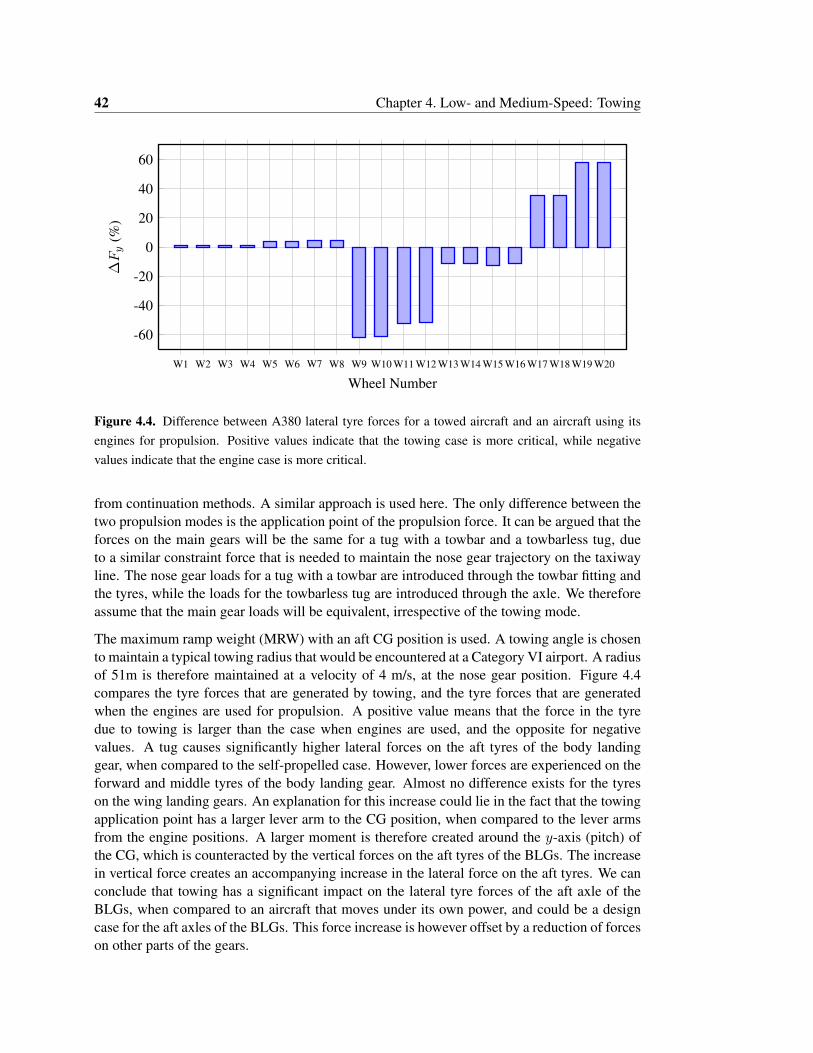
42 Chapter 4. Low- and Medium-Speed: Towing
W1 W2 W3 W4 W5 W6 W7 W8 W9 W10 W11 W12 W13 W14 W15 W16 W17 W18 W19 W20
-60
-40
-20
0
20
40
60
Wheel Number
∆Fy
(%)
Figure 4.4. Difference between A380 lateral tyre forces for a towed aircraft and an aircraft using itsengines for propulsion. Positive values indicate that the towing case is more critical, while negativevalues indicate that the engine case is more critical.
from continuation methods. A similar approach is used here. The only difference between thetwo propulsion modes is the application point of the propulsion force. It can be argued that theforces on the main gears will be the same for a tug with a towbar and a towbarless tug, dueto a similar constraint force that is needed to maintain the nose gear trajectory on the taxiwayline. The nose gear loads for a tug with a towbar are introduced through the towbar fitting andthe tyres, while the loads for the towbarless tug are introduced through the axle. We thereforeassume that the main gear loads will be equivalent, irrespective of the towing mode.
The maximum ramp weight (MRW) with an aft CG position is used. A towing angle is chosento maintain a typical towing radius that would be encountered at a Category VI airport. A radiusof 51m is therefore maintained at a velocity of 4 m/s, at the nose gear position. Figure 4.4compares the tyre forces that are generated by towing, and the tyre forces that are generatedwhen the engines are used for propulsion. A positive value means that the force in the tyredue to towing is larger than the case when engines are used, and the opposite for negativevalues. A tug causes significantly higher lateral forces on the aft tyres of the body landinggear, when compared to the self-propelled case. However, lower forces are experienced on theforward and middle tyres of the body landing gear. Almost no difference exists for the tyreson the wing landing gears. An explanation for this increase could lie in the fact that the towingapplication point has a larger lever arm to the CG position, when compared to the lever armsfrom the engine positions. A larger moment is therefore created around the y-axis (pitch) ofthe CG, which is counteracted by the vertical forces on the aft tyres of the BLGs. The increasein vertical force creates an accompanying increase in the lateral force on the aft tyres. We canconclude that towing has a significant impact on the lateral tyre forces of the aft axle of theBLGs, when compared to an aircraft that moves under its own power, and could be a designcase for the aft axles of the BLGs. This force increase is however offset by a reduction of forceson other parts of the gears.
4.4. Discussion 43
4.4 Discussion
We presented a physical interpretation of towing manoeuvres, starting from the fact that push-back manoeuvres are inherently unstable. We also concluded that jackknifing can be avoidedby maintaining a towing radius that is larger than the wheel base. Even though no detailed dy-namic analysis was conducted, useful rules for towing and control purposes are derived fromthe kinematics of towing, which builds on previous work by Fossum et al. [25]. These rulescan be used to determine what effect certain landing gear configurations might have when anaircraft is being towed around specific airports. Detailed dynamic models are needed if theeffects of low friction surfaces (such as oil on concrete) are to be studied.
This was followed by a comparison between the tyre forces that are generated when the noselanding gear follows a circular trajectory – equivalent to an exit radius – under its own power,and when the aircraft is towed at an equivalent circular trajectory by a towbarless tug. Weassumed that a comparison of the steady-state forces would be sufficient, and that towbarlesstowing would generate the same forces as a towtruck with a towbar. Continuation methodsprovide such steady-state information quickly and efficiently. It was shown that the aft tyres ofthe body landing gear experience significantly higher loads for the towing case due to a largerlever arm with respect to the CG position, when compared to the shorter lever arms of theengine positions. The tyres on the wing landing gear experience lower forces, when comparedto the self-propelled case. We can therefore conclude that towbarless towing could be a designcase for the aft axle of the body landing gear, which is offset by load alleviation on other partsof the gear.

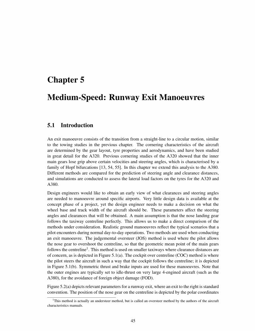
Chapter 5
Medium-Speed: Runway Exit Manoeuvres
5.1 Introduction
An exit manoeuvre consists of the transition from a straight-line to a circular motion, similarto the towing studies in the previous chapter. The cornering characteristics of the aircraftare determined by the gear layout, tyre properties and aerodynamics, and have been studiedin great detail for the A320. Previous cornering studies of the A320 showed that the innermain gears lose grip above certain velocities and steering angles, which is characterised by afamily of Hopf bifurcations [13, 54, 55]. In this chapter we extend this analysis to the A380.Different methods are compared for the prediction of steering angle and clearance distances,and simulations are conducted to assess the lateral load factors on the tyres for the A320 andA380.
Design engineers would like to obtain an early view of what clearances and steering anglesare needed to manoeuvre around specific airports. Very little design data is available at theconcept phase of a project, yet the design engineer needs to make a decision on what thewheel base and track width of the aircraft should be. These parameters affect the steeringangles and clearances that will be obtained. A main assumption is that the nose landing gearfollows the taxiway centreline perfectly. This allows us to make a direct comparison of themethods under consideration. Realistic ground manoeuvres reflect the typical scenarios that apilot encounters during normal day-to-day operations. Two methods are used when conductingan exit manoeuvre. The judgemental oversteer (JOS) method is used where the pilot allowsthe nose gear to overshoot the centreline, so that the geometric mean point of the main gearsfollows the centreline1. This method is used on smaller taxiways where clearance distances areof concern, as is depicted in Figure 5.1(a). The cockpit over centreline (COC) method is wherethe pilot steers the aircraft in such a way that the cockpit follows the centreline; it is depictedin Figure 5.1(b). Symmetric thrust and brake inputs are used for these manoeuvres. Note thatthe outer engines are typically set to idle-thrust on very large 4-engined aircraft (such as theA380), for the avoidance of foreign object damage (FOD).
Figure 5.2(a) depicts relevant parameters for a runway exit, where an exit to the right is standardconvention. The position of the nose gear on the centreline is depicted by the polar coordinates
1This method is actually an understeer method, but is called an oversteer method by the authors of the aircraftcharacteristics manuals.
45
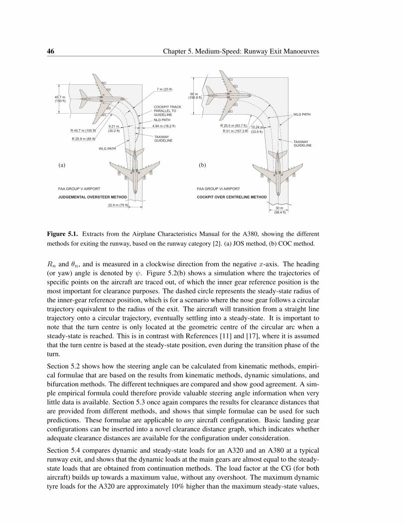
46 Chapter 5. Medium-Speed: Runway Exit Manoeuvres
NLG PATH
COCKPIT TRACKPARALLEL TOGUIDELINE
TAXIWAYGUIDELINE
WLG PATH
9.21 m 4.94 m (16.2 ft)
45.7 m(150 ft)
R 45.7 m (150 ft)
R 25.9 m (85 ft)
(30.2 ft)
7 m (23 ft)
22.9 m (75 ft)
TAXIWAYGUIDELINE
WLG PATH
60 m(196.9 ft)
R 25.5 m (83.7 ft)
R 51 m (167.3 ft)10.24 m
(33.6 ft)
30 m
(98.4 ft)
FAA GROUP VI AIRPORT
COCKPIT OVER CENTRELINE METHOD
FAA GROUP V AIRPORT
JUDGEMENTAL OVERSTEER METHOD
(a) (b)
Figure 5.1. Extracts from the Airplane Characteristics Manual for the A380, showing the differentmethods for exiting the runway, based on the runway category [2]. (a) JOS method, (b) COC method.
Rn and θn, and is measured in a clockwise direction from the negative x-axis. The heading(or yaw) angle is denoted by ψ. Figure 5.2(b) shows a simulation where the trajectories ofspecific points on the aircraft are traced out, of which the inner gear reference position is themost important for clearance purposes. The dashed circle represents the steady-state radius ofthe inner-gear reference position, which is for a scenario where the nose gear follows a circulartrajectory equivalent to the radius of the exit. The aircraft will transition from a straight linetrajectory onto a circular trajectory, eventually settling into a steady-state. It is important tonote that the turn centre is only located at the geometric centre of the circular arc when asteady-state is reached. This is in contrast with References [11] and [17], where it is assumedthat the turn centre is based at the steady-state position, even during the transition phase of theturn.
Section 5.2 shows how the steering angle can be calculated from kinematic methods, empiri-cal formulae that are based on the results from kinematic methods, dynamic simulations, andbifurcation methods. The different techniques are compared and show good agreement. A sim-ple empirical formula could therefore provide valuable steering angle information when verylittle data is available. Section 5.3 once again compares the results for clearance distances thatare provided from different methods, and shows that simple formulae can be used for suchpredictions. These formulae are applicable to any aircraft configuration. Basic landing gearconfigurations can be inserted into a novel clearance distance graph, which indicates whetheradequate clearance distances are available for the configuration under consideration.
Section 5.4 compares dynamic and steady-state loads for an A320 and an A380 at a typicalrunway exit, and shows that the dynamic loads at the main gears are almost equal to the steady-state loads that are obtained from continuation methods. The load factor at the CG (for bothaircraft) builds up towards a maximum value, without any overshoot. The maximum dynamictyre loads for the A320 are approximately 10% higher than the maximum steady-state values,
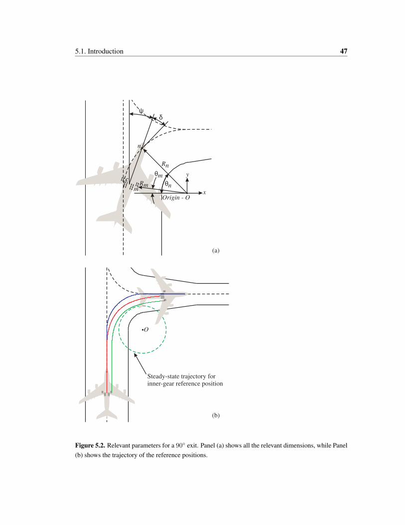
5.1. Introduction 47
θn
δ
Rn
Rm
n
cc
m
(a)
(b)
Steady-state trajectory forinner-gear reference position
θm
Origin - O
O
x
y
ψ
Figure 5.2. Relevant parameters for a 90◦ exit. Panel (a) shows all the relevant dimensions, while Panel(b) shows the trajectory of the reference positions.
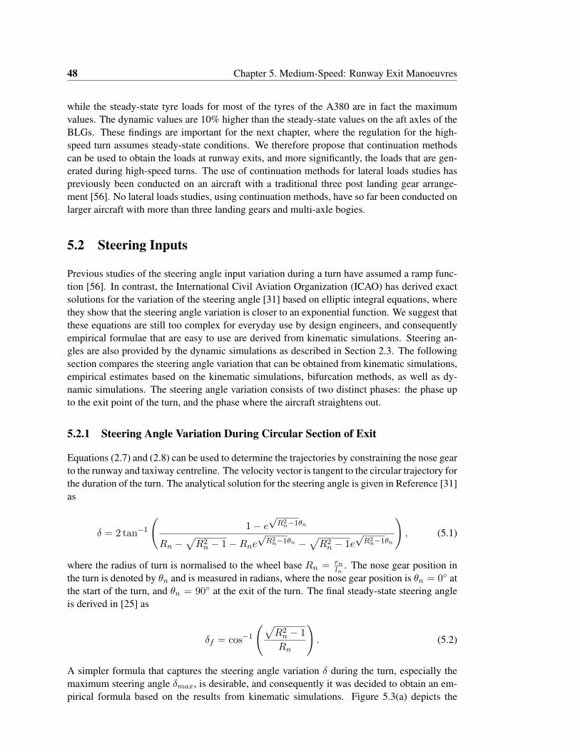
48 Chapter 5. Medium-Speed: Runway Exit Manoeuvres
while the steady-state tyre loads for most of the tyres of the A380 are in fact the maximumvalues. The dynamic values are 10% higher than the steady-state values on the aft axles of theBLGs. These findings are important for the next chapter, where the regulation for the high-speed turn assumes steady-state conditions. We therefore propose that continuation methodscan be used to obtain the loads at runway exits, and more significantly, the loads that are gen-erated during high-speed turns. The use of continuation methods for lateral loads studies haspreviously been conducted on an aircraft with a traditional three post landing gear arrange-ment [56]. No lateral loads studies, using continuation methods, have so far been conducted onlarger aircraft with more than three landing gears and multi-axle bogies.
5.2 Steering Inputs
Previous studies of the steering angle input variation during a turn have assumed a ramp func-tion [56]. In contrast, the International Civil Aviation Organization (ICAO) has derived exactsolutions for the variation of the steering angle [31] based on elliptic integral equations, wherethey show that the steering angle variation is closer to an exponential function. We suggest thatthese equations are still too complex for everyday use by design engineers, and consequentlyempirical formulae that are easy to use are derived from kinematic simulations. Steering an-gles are also provided by the dynamic simulations as described in Section 2.3. The followingsection compares the steering angle variation that can be obtained from kinematic simulations,empirical estimates based on the kinematic simulations, bifurcation methods, as well as dy-namic simulations. The steering angle variation consists of two distinct phases: the phase upto the exit point of the turn, and the phase where the aircraft straightens out.
5.2.1 Steering Angle Variation During Circular Section of Exit
Equations (2.7) and (2.8) can be used to determine the trajectories by constraining the nose gearto the runway and taxiway centreline. The velocity vector is tangent to the circular trajectory forthe duration of the turn. The analytical solution for the steering angle is given in Reference [31]as
δ = 2 tan−1
(1− e
√R2
n−1θn
Rn −√R2n − 1−Rne
√R2
n−1θn −√R2n − 1e
√R2
n−1θn
), (5.1)
where the radius of turn is normalised to the wheel base Rn = rnln
. The nose gear position inthe turn is denoted by θn and is measured in radians, where the nose gear position is θn = 0◦ atthe start of the turn, and θn = 90◦ at the exit of the turn. The final steady-state steering angleis derived in [25] as
δf = cos−1
(√R2n − 1
Rn
). (5.2)
A simpler formula that captures the steering angle variation δ during the turn, especially themaximum steering angle δmax, is desirable, and consequently it was decided to obtain an em-pirical formula based on the results from kinematic simulations. Figure 5.3(a) depicts the
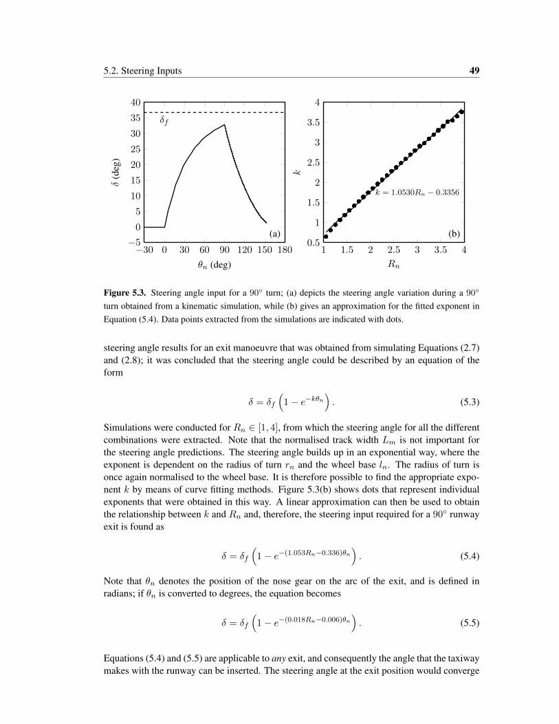
5.2. Steering Inputs 49
−30 0 30 60 90 120 150 180−5
0
5
10
15
20
25
30
35
40
(a)
δf
θn (deg)
δ(d
eg)
1 1.5 2 2.5 3 3.5 40.5
1
1.5
2
2.5
3
3.5
4
(b)
k = 1.0530Rn − 0.3356
Rn
kFigure 5.3. Steering angle input for a 90◦ turn; (a) depicts the steering angle variation during a 90◦
turn obtained from a kinematic simulation, while (b) gives an approximation for the fitted exponent inEquation (5.4). Data points extracted from the simulations are indicated with dots.
steering angle results for an exit manoeuvre that was obtained from simulating Equations (2.7)and (2.8); it was concluded that the steering angle could be described by an equation of theform
δ = δf
(1− e−kθn
). (5.3)
Simulations were conducted for Rn ∈ [1, 4], from which the steering angle for all the differentcombinations were extracted. Note that the normalised track width Lm is not important forthe steering angle predictions. The steering angle builds up in an exponential way, where theexponent is dependent on the radius of turn rn and the wheel base ln. The radius of turn isonce again normalised to the wheel base. It is therefore possible to find the appropriate expo-nent k by means of curve fitting methods. Figure 5.3(b) shows dots that represent individualexponents that were obtained in this way. A linear approximation can then be used to obtainthe relationship between k and Rn and, therefore, the steering input required for a 90◦ runwayexit is found as
δ = δf
(1− e−(1.053Rn−0.336)θn
). (5.4)
Note that θn denotes the position of the nose gear on the arc of the exit, and is defined inradians; if θn is converted to degrees, the equation becomes
δ = δf
(1− e−(0.018Rn−0.006)θn
). (5.5)
Equations (5.4) and (5.5) are applicable to any exit, and consequently the angle that the taxiwaymakes with the runway can be inserted. The steering angle at the exit position would converge
50 Chapter 5. Medium-Speed: Runway Exit Manoeuvres
10 20 30 400
10
20
30
40
50
(a)
Wheel base ln (m)
δ(d
eg)
Steady-state135◦ Exit90◦ Exit
10 20 30 400
10
20
30
40
50
(b)
Wheel base ln (m)δ
(deg
)
Steady-state135◦ Exit90◦ Exit
Figure 5.4. Maximum steering angle inputs for, (a) Category V and, (b) Category VI airports.
towards the steady-state steering angle as the exit radius is increased, or as the wheel base isdecreased; the latter can be seen clearly in Figures 5.4(a) and 5.4(b). These graphs can be usedto estimate the steering angle requirements for any aircraft configuration, where Appendix Ccontains steering angle calculations for different aircraft types. The position of the nose gearon the circular trajectory can be converted to the time domain to yield
δ = δf
(1− e−(1.053Rn−0.336) Vn
Rnt). (5.6)
The velocity is normalised to the wheel base and is expressed as wheel base lengths per second.It is assumed that the velocity during the turn stays constant, which is not a realistic scenariofor a constant thrust configuration, as the velocity will decrease as the turn progresses [56]. Thesteady-state velocity for a specific steering angle can be obtained from a bifurcation diagram,and consequently an average velocity can be derived for Equation (5.6). From simple geometryin Figure 5.2, it can easily be shown that the heading angle ψ is the difference between theangular position of the nose gear on the circular trajectory, θn, and the steering angle δ. At theexit from the turn where θn = 90◦, the heading angle becomes
ψ90 = 90◦ − δ90 (deg). (5.7)
5.2.2 Steering Angle Variation on Horizontal Section of Exit
The change in steering angle when the aircraft nose gear is moving on a horizontal line (x-direction) forms a tractrix [31]; it can be derived from the y-coordinate of the main gear refer-ence position cy, which is calculated as [25]
cy(t) =(k − 1) sin(ψ90 + 180◦)
ket − e−t. (5.8)
5.2. Steering Inputs 51
The next step is to apply the initial conditions at the exit, thus when θn = 90◦. Set t = 0, andinsert the heading angle from Equation (5.7) at the exit ψ90. The factor k is derived as
k =cos(ψ90)− 1
cos(ψ90) + 1. (5.9)
The steering angle can then be calculated in the time domain as
δ(t) = sin−1(cy(t)). (5.10)
Design engineers are more interested in the maximum steering angle and the steering rate,hence, the need for a simplified equation in the previous section. No attempt will be made toderive a simpler equation describing the decrease in steering angle from the exit, as this is nota critical part of the manoeuvre.
5.2.3 Steering Angle Predictions from Continuation Methods
The previous empirical and kinematic methods described above are adequate for calculating thetowing angles during the preliminary and detail design phases. The steering angle predictionsare similar to the towing predictions during the preliminary design phase, but do need to berefined for the detail design phase. Section 5.2.1 showed that a turn manoeuvre consists of atransition between a straight line and a circular manoeuvre, and that the steady-state solutionof the steering angle can be used in Equation (5.4). This steady-state steering angle is howeverbased on geometric methods, which ignore the tyre and aircraft dynamics.
Bifurcation methods, and more specifically, continuation methods, can provide the steady-statesteering angle for different aircraft configurations, meaning that the tyre properties are takeninto consideration [15]. The question is whether continuation methods provide a more accurateestimate of the steering profile compared to geometric methods. If so, the accuracy of thesteering angle prediction can be improved at a smaller computational cost, compared to fulldynamic simulations. Chapter 3 showed how a SimMechanics model of the A380 can be usedwith the Dynamical Systems Toolbox for the prediction of turn widths pertaining to U-turnmanoeuvres. The same method is used here for the prediction of steering angles.
The turn radius can be calculated by dividing the velocity at the nose gear by the yaw rate; boththese states are provided by the continuation analysis. Figure 5.5(a) shows the variation of theturn radius as the steering angle is increased for a velocity of 3 m/s. The steady-state steeringangle that will provide a turn radius of 51 metres for Group VI airport taxiway turns can beobtained from the graph. In this case a steering angle of 37.9◦ will provide the required turnradius.
5.2.4 Steering Angle Comparisons for the Different Methods
The pilot will usually try to maintain momentum (hence velocity) during the turn, by adjust-ing the thrust. Future automated systems are also likely to maintain a specific velocity profileduring a turn, of which a constant velocity could be one of the candidates. A constant velocity
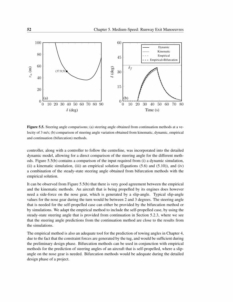
52 Chapter 5. Medium-Speed: Runway Exit Manoeuvres
0 10 20 30 40 50 60 70 80 900
20
40
60
80
100
(a)
a(37.9,51)
δ (deg)
r n(m
)
0 10 20 30 40 50 60 70 800
15
30
45
60
(b)
δf
Time (s)δ
(deg
)
DynamicKinematicEmpirical
Empirical+Bifurcation
Figure 5.5. Steering angle comparisons; (a) steering angle obtained from continuation methods at a ve-locity of 3 m/s; (b) comparison of steering angle variation obtained from kinematic, dynamic, empiricaland continuation (bifurcation) methods.
controller, along with a controller to follow the centreline, was incorporated into the detaileddynamic model, allowing for a direct comparison of the steering angle for the different meth-ods. Figure 5.5(b) contains a comparison of the input required from (i) a dynamic simulation,(ii) a kinematic simulation, (iii) an empirical solution (Equations (5.6) and (5.10)), and (iv)a combination of the steady-state steering angle obtained from bifurcation methods with theempirical solution.
It can be observed from Figure 5.5(b) that there is very good agreement between the empiricaland the kinematic methods. An aircraft that is being propelled by its engines does howeverneed a side-force on the nose gear, which is generated by a slip-angle. Typical slip-anglevalues for the nose gear during the turn would be between 2 and 3 degrees. The steering anglethat is needed for the self-propelled case can either be provided by the bifurcation method orby simulations. We adapt the empirical method to include the self-propelled case, by using thesteady-state steering angle that is provided from continuation in Section 5.2.3, where we seethat the steering angle predictions from the continuation method are close to the results fromthe simulations.
The empirical method is also an adequate tool for the prediction of towing angles in Chapter 4,due to the fact that the constraint forces are generated by the tug, and would be sufficient duringthe preliminary design phase. Bifurcation methods can be used in conjunction with empiricalmethods for the prediction of steering angles of an aircraft that is self-propelled, where a slip-angle on the nose gear is needed. Bifurcation methods would be adequate during the detaileddesign phase of a project.
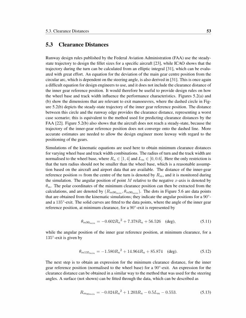
5.3. Clearance Distances 53
5.3 Clearance Distances
Runway design rules published by the Federal Aviation Administration (FAA) use the steady-state trajectory to design the fillet sizes for a specific aircraft [23], while ICAO shows that thetrajectory during the turn can be calculated from an elliptic integral [31], which can be evalu-ated with great effort. An equation for the deviation of the main gear centre position from thecircular arc, which is dependent on the steering angle, is also derived in [31]. This is once againa difficult equation for design engineers to use, and it does not include the clearance distance ofthe inner gear reference position. It would therefore be useful to provide design rules on howthe wheel base and track width influence the performance characteristics. Figures 5.2(a) and(b) show the dimensions that are relevant to exit manoeuvres, where the dashed circle in Fig-ure 5.2(b) depicts the steady-state trajectory of the inner gear reference position. The distancebetween this circle and the runway edge provides the clearance distance, representing a worstcase scenario; this is equivalent to the method used for predicting clearance distances by theFAA [22]. Figure 5.2(b) also shows that the aircraft does not reach a steady-state, because thetrajectory of the inner-gear reference position does not converge onto the dashed line. Moreaccurate estimates are needed to allow the design engineer more leeway with regard to thepositioning of the gears.
Simulations of the kinematic equations are used here to obtain minimum clearance distancesfor varying wheel base and track width combinations. The radius of turn and the track width arenormalised to the wheel base, where Rn ∈ [1, 4] and Lm ∈ [0, 0.6]. Here the only restriction isthat the turn radius should not be smaller than the wheel base, which is a reasonable assump-tion based on the aircraft and airport data that are available. The distance of the inner-gearreference position m from the centre of the turn is denoted by Rm, and it is monitored duringthe simulation. The angular position of point M relative to the negative x-axis is denoted byθm. The polar coordinates of the minimum clearance position can then be extracted from thecalculations, and are denoted by (Rm90min , θm90min). The dots in Figure 5.6 are data pointsthat are obtained from the kinematic simulations; they indicate the angular positions for a 90◦-and a 135◦-exit. The solid curves are fitted to the data points, where the angle of the inner gearreference position, at minimum clearance, for a 90◦-exit is represented by
θm90min = −0.602Rn2 + 7.378Rn + 56.526 (deg), (5.11)
while the angular position of the inner gear reference position, at minimum clearance, for a135◦-exit is given by
θm135min = −1.580Rn2 + 14.964Rn + 85.874 (deg). (5.12)
The next step is to obtain an expression for the minimum clearance distance, for the innergear reference position (normalised to the wheel base) for a 90◦-exit. An expression for theclearance distance can be obtained in a similar way to the method that was used for the steeringangles. A surface (not shown) can be fitted through the data, which can be described as
Rm90min = −0.024Rn2 + 1.203Rn − 0.5Lm − 0.553. (5.13)
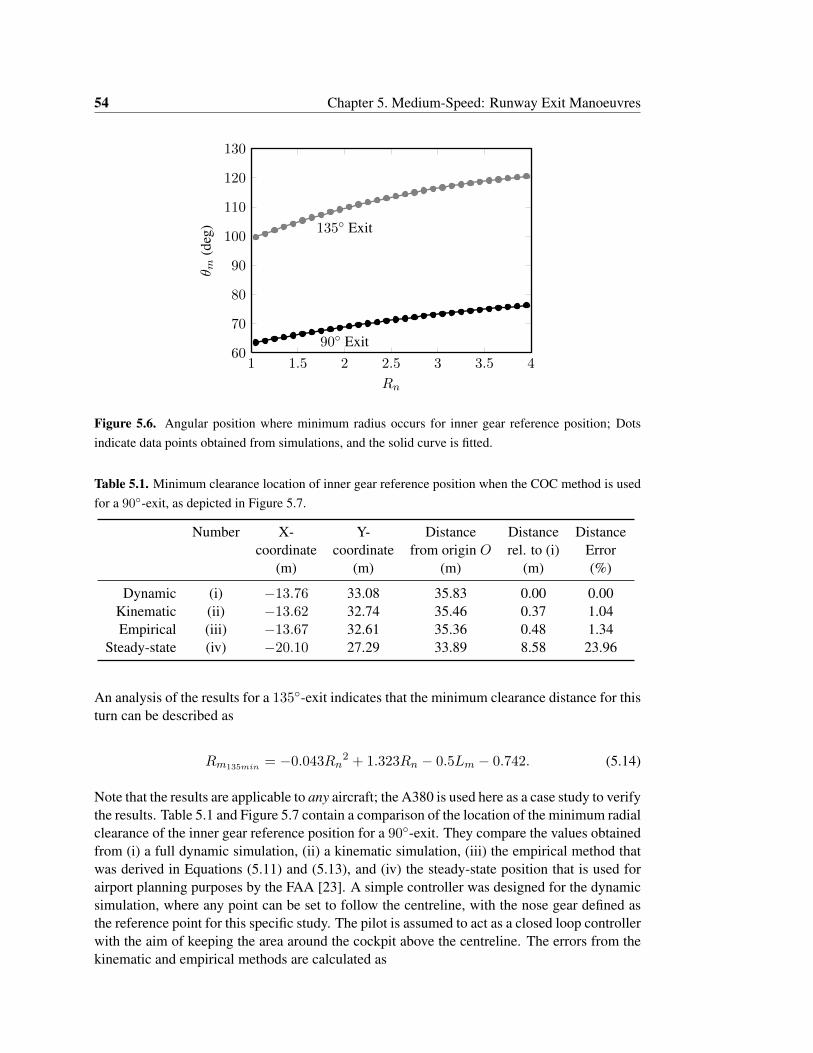
54 Chapter 5. Medium-Speed: Runway Exit Manoeuvres
1 1.5 2 2.5 3 3.5 460
70
80
90
100
110
120
130
90◦ Exit
135◦ Exit
Rn
θ m(d
eg)
Figure 5.6. Angular position where minimum radius occurs for inner gear reference position; Dotsindicate data points obtained from simulations, and the solid curve is fitted.
Table 5.1. Minimum clearance location of inner gear reference position when the COC method is usedfor a 90◦-exit, as depicted in Figure 5.7.
Number X- Y- Distance Distance Distancecoordinate coordinate from origin O rel. to (i) Error
(m) (m) (m) (m) (%)
Dynamic (i) −13.76 33.08 35.83 0.00 0.00Kinematic (ii) −13.62 32.74 35.46 0.37 1.04Empirical (iii) −13.67 32.61 35.36 0.48 1.34
Steady-state (iv) −20.10 27.29 33.89 8.58 23.96
An analysis of the results for a 135◦-exit indicates that the minimum clearance distance for thisturn can be described as
Rm135min = −0.043Rn2 + 1.323Rn − 0.5Lm − 0.742. (5.14)
Note that the results are applicable to any aircraft; the A380 is used here as a case study to verifythe results. Table 5.1 and Figure 5.7 contain a comparison of the location of the minimum radialclearance of the inner gear reference position for a 90◦-exit. They compare the values obtainedfrom (i) a full dynamic simulation, (ii) a kinematic simulation, (iii) the empirical method thatwas derived in Equations (5.11) and (5.13), and (iv) the steady-state position that is used forairport planning purposes by the FAA [23]. A simple controller was designed for the dynamicsimulation, where any point can be set to follow the centreline, with the nose gear defined asthe reference point for this specific study. The pilot is assumed to act as a closed loop controllerwith the aim of keeping the area around the cockpit above the centreline. The errors from thekinematic and empirical methods are calculated as
5.4. Load Factors During Runway Exit Turns 55
e = 1− Mimin −Mjmin
|Mimin |. (5.15)
Following the convention in Figure 2.3, where M is the position vector of the inner-gear refer-ence position, Mimin denotes the minimum radius vector position for the dynamic simulationcase. The other positions are denoted by Mjmin where j represents the label of the case underconsideration. The results from the empirical predictions are within 1.5% of the results fromthe dynamic simulations. It can be concluded from Figure 5.7 that Equation (5.13) gives a goodestimate of the clearance distance that can be achieved for a 90◦-exit; in particular, the estimateis significantly better than the steady-state approximation. The same holds true for the 135◦
case, although the minimum radial distance is close to the steady-state value.
Feasible wheel base and track width combinations can be determined by inserting a minimumradial distance into Equations (5.13) and (5.14), and then recasting the equations so that thetrack width appears on the left-hand side. The fillet radius for Group V and VI airports is as-sumed to be 25.9 metres [2], where a minimum clearance distance of 4.5 metres is needed [31].The locus of track widths that provide a radius of 30.4 metres will therefore provide the bound-ary for the feasible region of wheel base and track widths. Appendix C contains clearancedistances for different aircraft types.
Figure 5.8 depicts such an envelope for the different types of airports and exits. The area to theright of a hatched line indicates a clearance distance of less than 4.5 metres for the particularcase. The wheel base that is depicted on the x-axis could also be replaced by the distance fromthe cockpit to the main gear reference position, which would represent the COC method. Wehave assumed that the nose gear will follow the centreline. It is possible to overlay the datafor any aircraft onto the graph, making the method useful for comparative purposes. We haveoverlaid the data (given in Appendix C), and it can be seen that the COC minimum clearancedistance for the A380 lies to the right of the required margins for Group V airports, hence theJOS method needs to be employed for this type of airport; this is consistent with the AirplaneCharacteristics Manual for the A380 [2], contained in Figure 5.1. Note the data point for theB747-8, for which it is predicted that the aircraft will have sufficient clearance on a Group Vairport with a 90◦ exit, but not for a 135◦ exit. It can be concluded that Figure 5.8 can be usedas a useful design tool at the early stages of an aircraft programme. On the other hand, thefinal clearance distances that are published in the Aircraft Characteristics Manual should stillbe obtained from detailed dynamic simulations.
5.4 Load Factors During Runway Exit Turns
The following section explores how the International Civil Aviation Organization (ICAO) de-termines the maximum exit velocity at a runway exit. Dynamic simulations of the A320 andA380 are then conducted at a typical runway exit in the sections thereafter. The results are alsocompared to steady-state values that are obtained from continuation analysis. These results areof importance for the assumptions that are made in Section 4.3 related to towing, as well asthe following chapter, which studies the lateral loads that can be obtained during high-speedturns. The regulatory cases for lateral loading do not specify any dynamic behaviour duringa turn. Rather, they only specify that the aircraft needs to be configured in such a way that a
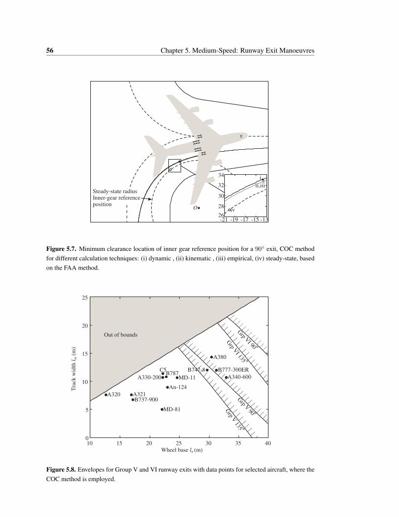
56 Chapter 5. Medium-Speed: Runway Exit Manoeuvres
i
iv
ii,iii
-13-15-17-19-21
Steady-state radiusInner-gear referenceposition
26
28
30
32
34
O
Figure 5.7. Minimum clearance location of inner gear reference position for a 90◦ exit, COC methodfor different calculation techniques: (i) dynamic , (ii) kinematic , (iii) empirical, (iv) steady-state, basedon the FAA method.
10 15 20 25 30 35 400
5
10
15
20
25
Grp
VI 90°
Grp
VI 135 °
Grp
V90°
Grp
V135 °
A320 A321
A330-200 A340-600
A380
B737-900
B747-8 B777-300ERB787
Wheel base ln (m)
Tra
ck w
idth
l m(m
)
Out of bounds
An-124
C5
MD-81
MD-11
Figure 5.8. Envelopes for Group V and VI runway exits with data points for selected aircraft, where theCOC method is employed.
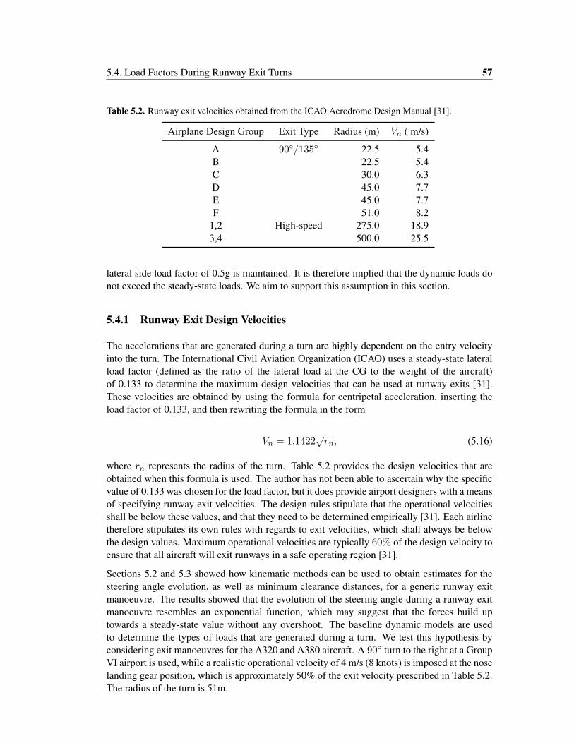
5.4. Load Factors During Runway Exit Turns 57
Table 5.2. Runway exit velocities obtained from the ICAO Aerodrome Design Manual [31].
Airplane Design Group Exit Type Radius (m) Vn ( m/s)
A 90◦/135◦ 22.5 5.4B 22.5 5.4C 30.0 6.3D 45.0 7.7E 45.0 7.7F 51.0 8.2
1,2 High-speed 275.0 18.93,4 500.0 25.5
lateral side load factor of 0.5g is maintained. It is therefore implied that the dynamic loads donot exceed the steady-state loads. We aim to support this assumption in this section.
5.4.1 Runway Exit Design Velocities
The accelerations that are generated during a turn are highly dependent on the entry velocityinto the turn. The International Civil Aviation Organization (ICAO) uses a steady-state lateralload factor (defined as the ratio of the lateral load at the CG to the weight of the aircraft)of 0.133 to determine the maximum design velocities that can be used at runway exits [31].These velocities are obtained by using the formula for centripetal acceleration, inserting theload factor of 0.133, and then rewriting the formula in the form
Vn = 1.1422√rn, (5.16)
where rn represents the radius of the turn. Table 5.2 provides the design velocities that areobtained when this formula is used. The author has not been able to ascertain why the specificvalue of 0.133 was chosen for the load factor, but it does provide airport designers with a meansof specifying runway exit velocities. The design rules stipulate that the operational velocitiesshall be below these values, and that they need to be determined empirically [31]. Each airlinetherefore stipulates its own rules with regards to exit velocities, which shall always be belowthe design values. Maximum operational velocities are typically 60% of the design velocity toensure that all aircraft will exit runways in a safe operating region [31].
Sections 5.2 and 5.3 showed how kinematic methods can be used to obtain estimates for thesteering angle evolution, as well as minimum clearance distances, for a generic runway exitmanoeuvre. The results showed that the evolution of the steering angle during a runway exitmanoeuvre resembles an exponential function, which may suggest that the forces build uptowards a steady-state value without any overshoot. The baseline dynamic models are usedto determine the types of loads that are generated during a turn. We test this hypothesis byconsidering exit manoeuvres for the A320 and A380 aircraft. A 90◦ turn to the right at a GroupVI airport is used, while a realistic operational velocity of 4 m/s (8 knots) is imposed at the noselanding gear position, which is approximately 50% of the exit velocity prescribed in Table 5.2.The radius of the turn is 51m.
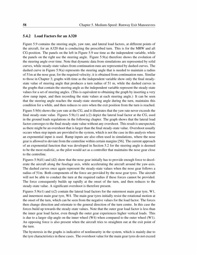
58 Chapter 5. Medium-Speed: Runway Exit Manoeuvres
5.4.2 Load Factors for an A320
Figure 5.9 contains the steering angle, yaw rate, and lateral load factors, at different points ofthe aircraft, for an A320 that is conducting the prescribed turn. This is for the MRW and aftCG-position. The panels on the left in Figure 5.9 use time as the independent variable, whilethe panels on the right use the steering angle. Figure 5.9(a) therefore shows the evolution ofthe steering angle over time. Note that dynamic data from simulations are represented by solidcurves, while steady-state values from continuation runs are represented by dashed curves. Thedashed curve in Figure 5.9(a) represents the steering angle that is needed to maintain a radiusof 51m at the nose gear, for the required velocity; it is obtained from continuation runs. Similarto those in Chapter 3; graphs with time as the independent variable show only the final steady-state value of steering angle that produces a turn radius of 51 m, while the dashed curves inthe graphs that contain the steering angle as the independent variable represent the steady-statevalues for a set of steering angles. (This is equivalent to obtaining the graph by inserting a veryslow ramp input, and then recording the state values at each steering angle.) It can be seenthat the steering angle reaches the steady-state steering angle during the turn, maintains thiscondition for a while, and then reduces to zero when the exit position from the turn is reached.
Figure 5.9(b) shows the yaw rate at the CG, and it illustrates that the yaw rate never exceeds thefinal steady-state value. Figures 5.9(c1) and (c2) depict the lateral load factor at the CG, usedin the ground loads regulations in the following chapter. The graph shows that the lateral loadfactor converges to the final steady-state value without any overshoot. This result is unexpected,as there might be an overshoot that is larger than the final steady-state value. Overshoot usuallyoccurs when step inputs are provided to the system, which is not the case in this analysis wherean exponential input is used. Ramp inputs are also often used in simulations, where the nosegear is allowed to deviate from the centreline within certain margins [56]. The current approachof an exponential function that was developed in Section 5.2 for the steering angle is deemedto be the most realistic, as the pilot would act as a controller that maintains the nose gear closeto the centreline.
Figures 5.9(d1) and (d2) show that the nose gear initially has to provide enough force to decel-erate the aircraft along the fuselage axis, while accelerating the aircraft around the yaw-axis.The dashed curves once again represent the steady-state values when the nose gear follows aradius of 51m. Both components of the force are provided by the nose gear tyres. The aircraftwill not be able to conduct the turn at the required radius if these forces cannot be provided.The force consequently builds up rapidly at the onset of the turn, and then reduces to thesteady-state value. A significant overshoot is therefore present.
Figures 5.9(e1) and (e2) contain the lateral load factors for the outermost main gear tyre, W1,and innermost main gear tyre, W4. The main gear tyres initially resist the rotational motion atthe onset of the turn, which can be seen from the negative values for the load factor. The forcesthen change direction and orientate to the general direction of the turn centre. In this case theforces build up towards the steady-state values. Note that the outer gear load factor is less thanthe inner gear load factor, even though the outer gear experiences higher vertical loads. Thisis due to a larger slip angle on the inner wheel (W4) when compared to the outer wheel (W1).An opposing force is also present when the aircraft tries to straighten out at the exit point ofthe turn.
The hysteresis in the graphs is indicative of nonlinearity in the system, which is mainly due tothe tyre characteristics in these cases. The overshoot value for the main gear tyres do not exceed
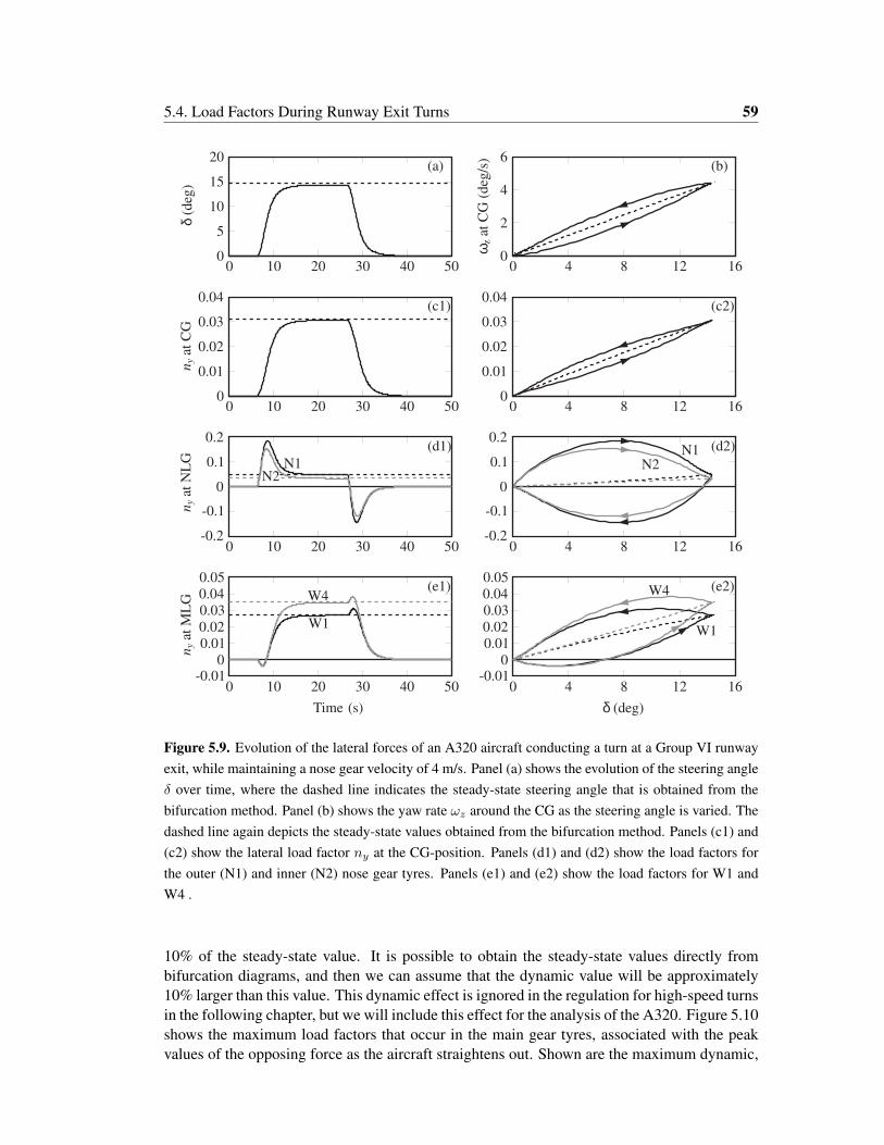
5.4. Load Factors During Runway Exit Turns 59
0 10 20 30 40 500
5
10
15
20(a)
0 4 8 12 160
2
4
6(b)
0 10 20 30 40 500
0.01
0.02
0.03
0.04(c1)
0 4 8 12 160
0.01
0.02
0.03
0.04(c2)
0 10 20 30 40 50-0.2
-0.1
0
0.1
0.2(d1)
0 4 8 12 16-0.2
-0.1
0
0.1
0.2(d2)
0 10 20 30 40 50
(e1)
Time (s)
0 4 8 12 16-0.01
0
0.01
0.02
0.03
0.04
0.05(e2)
-0.010
0.01
0.02
0.03
0.04
0.05
N1N2
W1
W4
N1N2
W1
W4
δ (deg)
δ(d
eg)
ωz
at C
G (
deg
/s)
ny
at C
Gn
yat
NL
Gn
yat
ML
G
Figure 5.9. Evolution of the lateral forces of an A320 aircraft conducting a turn at a Group VI runwayexit, while maintaining a nose gear velocity of 4 m/s. Panel (a) shows the evolution of the steering angleδ over time, where the dashed line indicates the steady-state steering angle that is obtained from thebifurcation method. Panel (b) shows the yaw rate ωz around the CG as the steering angle is varied. Thedashed line again depicts the steady-state values obtained from the bifurcation method. Panels (c1) and(c2) show the lateral load factor ny at the CG-position. Panels (d1) and (d2) show the load factors forthe outer (N1) and inner (N2) nose gear tyres. Panels (e1) and (e2) show the load factors for W1 andW4 .
10% of the steady-state value. It is possible to obtain the steady-state values directly frombifurcation diagrams, and then we can assume that the dynamic value will be approximately10% larger than this value. This dynamic effect is ignored in the regulation for high-speed turnsin the following chapter, but we will include this effect for the analysis of the A320. Figure 5.10shows the maximum load factors that occur in the main gear tyres, associated with the peakvalues of the opposing force as the aircraft straightens out. Shown are the maximum dynamic,
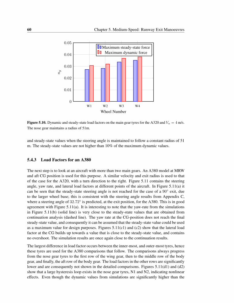
60 Chapter 5. Medium-Speed: Runway Exit Manoeuvres
W1 W2 W3 W40
0.01
0.02
0.03
0.04
0.05
Wheel Number
ny
Maximum steady-state forceMaximum dynamic force
Figure 5.10. Dynamic and steady-state load factors on the main gear tyres for the A320 and Vn = 4 m/s.The nose gear maintains a radius of 51m.
and steady-state values when the steering angle is maintained to follow a constant radius of 51m. The steady-state values are not higher than 10% of the maximum dynamic values.
5.4.3 Load Factors for an A380
The next step is to look at an aircraft with more than two main gears. An A380 model at MRWand aft CG position is used for this purpose. A similar velocity and exit radius is used to thatof the case for the A320, with a turn direction to the right. Figure 5.11 contains the steeringangle, yaw rate, and lateral load factors at different points of the aircraft. In Figure 5.11(a) itcan be seen that the steady-state steering angle is not reached for the case of a 90◦ exit, dueto the larger wheel base; this is consistent with the steering angle results from Appendix C,where a steering angle of 32.72◦ is predicted, at the exit position, for the A380. This is in goodagreement with Figure 5.11(a). It is interesting to note that the yaw-rate from the simulationsin Figure 5.11(b) (solid line) is very close to the steady-state values that are obtained fromcontinuation analysis (dashed line). The yaw rate at the CG-position does not reach the finalsteady-state value, and consequently it can be assumed that the steady-state value could be usedas a maximum value for design purposes. Figures 5.11(c1) and (c2) show that the lateral loadfactor at the CG builds up towards a value that is close to the steady-state value, and containsno overshoot. The simulation results are once again close to the continuation results.
The largest difference in load factor occurs between the inner-most, and outer-most tyres, hencethese tyres are used for the A380 comparisons that follow. The comparisons always progressfrom the nose gear tyres to the first row of the wing gear, then to the middle row of the bodygear, and finally, the aft row of the body gear. The load factors in the other rows are significantlylower and are consequently not shown in the detailed comparisons. Figures 5.11(d1) and (d2)show that a large hysteresis loop exists in the nose gear tyres, N1 and N2, indicating nonlineareffects. Even though the dynamic values from simulations are significantly higher than the
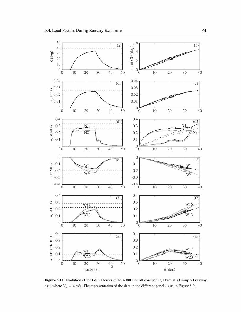
5.4. Load Factors During Runway Exit Turns 61
0 10 20 30 40 500
10
20
30
40
50(a)
0 10 20 30 400
2
4
6(b)
0 10 20 30 40 500
0.01
0.02
0.03
0.04(c1)
0 10 20 30 400
0.01
0.02
0.03
0.04(c2)
0 10 20 30 40 500
0.1
0.2
0.3
0.4(d1)
0 10 20 30 400
0.1
0.2
0.3
0.4(d2)
0 10 20 30 40 50-0.4
-0.3
-0.2
-0.1
0(e1)
0 10 20 30 40-0.4
-0.3
-0.2
-0.1
0(e2)
0 10 20 30 40 500
0.1
0.2
0.3
0.4(f1)
0 10 20 30 400
0.1
0.2
0.3
0.4(f2)
0 10 20 30 40 500
0.1
0.2
0.3
0.4(g1)
Time (s)
0 10 20 30 400
0.1
0.2
0 3:
0.4(g2)
2
δ(d
eg)
ny
at C
Gn
yat
NL
Gn
yat
ML
Gn
yat
BL
Gn
yA
ftA
xle
BL
G
ωz
at C
G (
deg
/s)
N1
N2
W1
W4
W16
W13
W17
W20
δ (deg)
N1
N2
W1
W4
W16
W13
W17
W20
Figure 5.11. Evolution of the lateral forces of an A380 aircraft conducting a turn at a Group VI runwayexit, where Vn = 4 m/s. The representation of the data in the different panels is as in Figure 5.9.
62 Chapter 5. Medium-Speed: Runway Exit Manoeuvres
steady-state values, they still do not exceed the steady-state values when a turn radius of 51mis maintained.
Figures 5.11(e1) and (e2) depict the load factors for tyres W1 and W4. Figure 5.11(e1) showsthat the final steady-state is not reached, while Figure 5.11(e2) shows that the dynamic valuesare close to the steady-state values during the turn. Figures 5.11(f1) and (f2) can be interpretedin a similar manner for W13 and W16. The tyres on the aft axle of the BLG, tyres W17 andW20, are shown in Figure 5.11(g1) and (g2), indicating similar load factors in both tyres. Thedynamic loads are also larger than the final steady-state value if a radius of 51m is maintained.The kink in the curves indicate the point where the body gear steering switches on, indicatingthat significant load relief can be obtained by adding steering onto the aft axles of the BLGs.Figure 5.11(g2) shows that the dynamic values are not far from the steady-state values.
Figure 5.12 contains the steady-state load factors on all 20 of the main gear tyres when the nosegear maintains a radius of 51m, and also the maximum dynamic load factor values for a 90◦
exit. The steady-state values are more critical for most of the tyres, apart from the tyres on theaft axles of the BLGs, where the maximum dynamic values are approximately 10% higher forthe aft axle wheels, when compared to the steady-state values. The overall steady-state loadson the BLGs are larger than the overall dynamic gear loads. The maximum tyre loads occurat the exit point from the turn (θ90) for W1-W16. The maximum for W17-W20 occurs afterθ90 when the aircraft straightens out. A similar pattern to that of the A320 emerges, where theinner tyres have a larger load factor compared to the outer tyres, even though the outer gearsexperience larger vertical loads.
We can therefore conclude that the dynamic load factors on the tyres of the A320 will beapproximately 10% higher than the steady-state values. This is in contrast to the A380, wherethe steady-state values are more critical for most of the tyres, which is consistent with theinterpretation of the lateral loads regulation in the following chapter. The previous chaptershowed that towing loads cause significantly higher loads in the aft tyres of the BLGs, hencethe dynamic effect on the aft axles of the BLGs are likely to be less important than for thetowing case. One could therefore use the steady-state loads on an aircraft such as the A380 fordesign purposes, and add a correction to incorporate the dynamic effect for a smaller aircraftsuch as the A320. Continuation analysis provides these steady-state values.
5.5 Discussion
An empirical formula that was derived from the results from kinematic simulations, was usedto evaluate the steering angle variation during a 90◦-exit manoeuvre. This empirical formulashowed very good agreement with kinematic and dynamic simulations. A steering input wasderived from a dynamic model with a controller for additional validation purposes, where thecontroller is used to maintain the nose landing gear on the taxiway centre line. The steeringangle obtained with the controller showed small differences from the steering angle obtainedfrom the kinematic method, due to a slip-angle that is needed when the dynamic method isused. This slip-angle is responsible for the generation of a side force that maintains the cir-cular trajectory of the nose landing gear. More accurate variations of the empirical formulacan be obtained, by adjusting the final steering angle. This adjustment can be obtained fromcontinuation; this is in close agreement with the values that are obtained from simulations. The
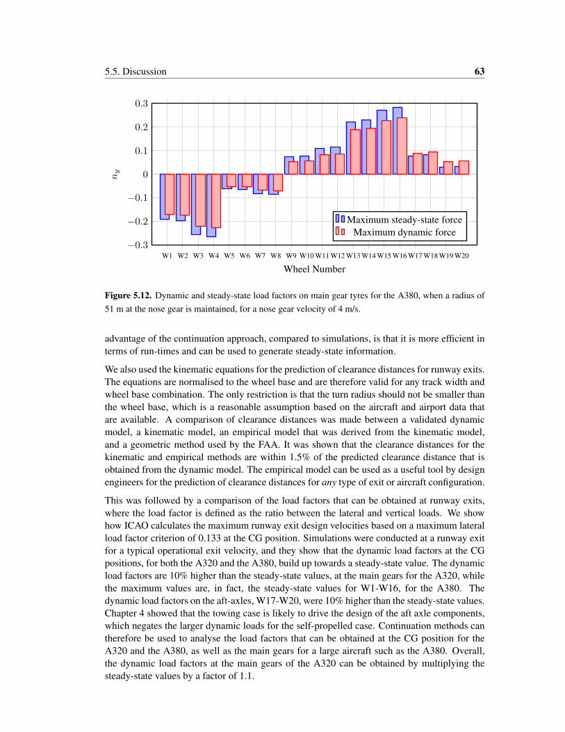
5.5. Discussion 63
W1 W2 W3 W4 W5 W6 W7 W8 W9 W10 W11 W12 W13 W14 W15 W16 W17 W18 W19 W20−0.3
−0.2
−0.1
0
0.1
0.2
0.3
Wheel Number
ny
Maximum steady-state forceMaximum dynamic force
Figure 5.12. Dynamic and steady-state load factors on main gear tyres for the A380, when a radius of51 m at the nose gear is maintained, for a nose gear velocity of 4 m/s.
advantage of the continuation approach, compared to simulations, is that it is more efficient interms of run-times and can be used to generate steady-state information.
We also used the kinematic equations for the prediction of clearance distances for runway exits.The equations are normalised to the wheel base and are therefore valid for any track width andwheel base combination. The only restriction is that the turn radius should not be smaller thanthe wheel base, which is a reasonable assumption based on the aircraft and airport data thatare available. A comparison of clearance distances was made between a validated dynamicmodel, a kinematic model, an empirical model that was derived from the kinematic model,and a geometric method used by the FAA. It was shown that the clearance distances for thekinematic and empirical methods are within 1.5% of the predicted clearance distance that isobtained from the dynamic model. The empirical model can be used as a useful tool by designengineers for the prediction of clearance distances for any type of exit or aircraft configuration.
This was followed by a comparison of the load factors that can be obtained at runway exits,where the load factor is defined as the ratio between the lateral and vertical loads. We showhow ICAO calculates the maximum runway exit design velocities based on a maximum lateralload factor criterion of 0.133 at the CG position. Simulations were conducted at a runway exitfor a typical operational exit velocity, and they show that the dynamic load factors at the CGpositions, for both the A320 and the A380, build up towards a steady-state value. The dynamicload factors are 10% higher than the steady-state values, at the main gears for the A320, whilethe maximum values are, in fact, the steady-state values for W1-W16, for the A380. Thedynamic load factors on the aft-axles, W17-W20, were 10% higher than the steady-state values.Chapter 4 showed that the towing case is likely to drive the design of the aft axle components,which negates the larger dynamic loads for the self-propelled case. Continuation methods cantherefore be used to analyse the load factors that can be obtained at the CG position for theA320 and the A380, as well as the main gears for a large aircraft such as the A380. Overall,the dynamic load factors at the main gears of the A320 can be obtained by multiplying thesteady-state values by a factor of 1.1.

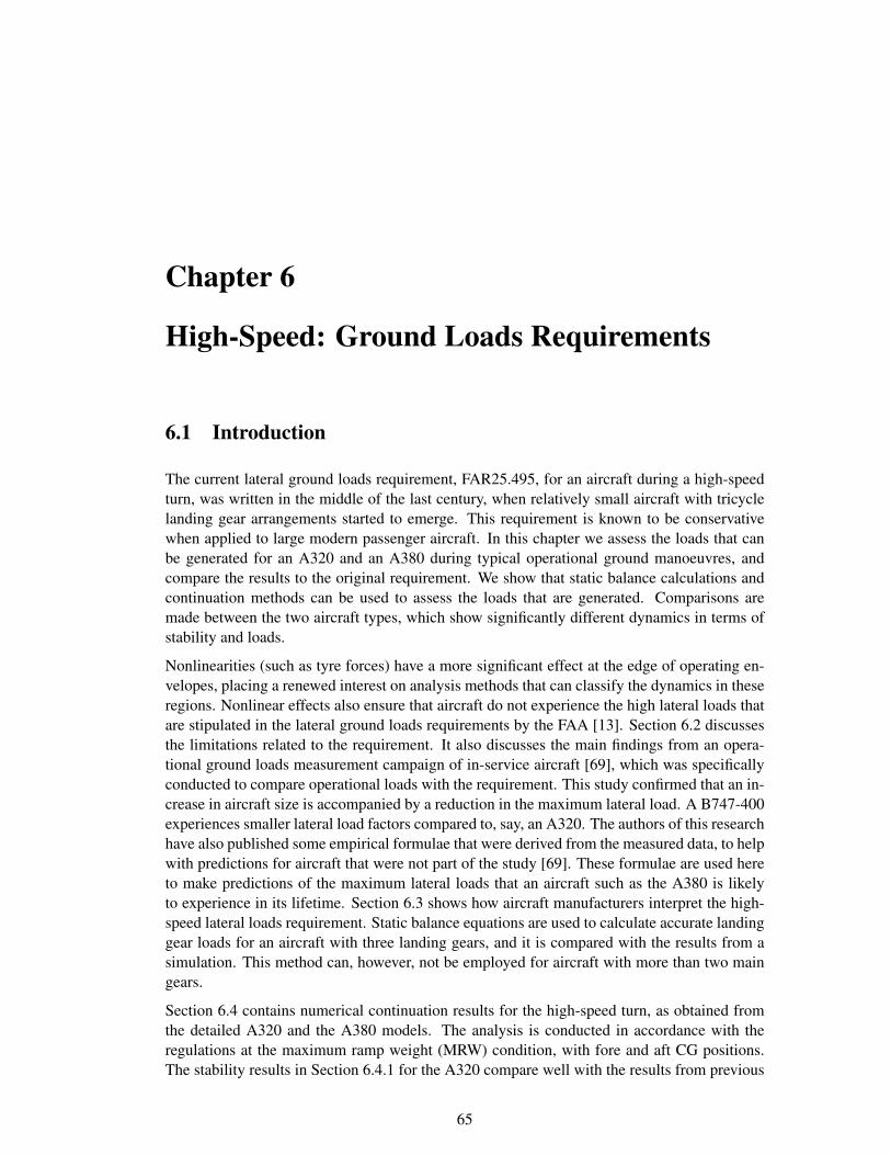
Chapter 6
High-Speed: Ground Loads Requirements
6.1 Introduction
The current lateral ground loads requirement, FAR25.495, for an aircraft during a high-speedturn, was written in the middle of the last century, when relatively small aircraft with tricyclelanding gear arrangements started to emerge. This requirement is known to be conservativewhen applied to large modern passenger aircraft. In this chapter we assess the loads that canbe generated for an A320 and an A380 during typical operational ground manoeuvres, andcompare the results to the original requirement. We show that static balance calculations andcontinuation methods can be used to assess the loads that are generated. Comparisons aremade between the two aircraft types, which show significantly different dynamics in terms ofstability and loads.
Nonlinearities (such as tyre forces) have a more significant effect at the edge of operating en-velopes, placing a renewed interest on analysis methods that can classify the dynamics in theseregions. Nonlinear effects also ensure that aircraft do not experience the high lateral loads thatare stipulated in the lateral ground loads requirements by the FAA [13]. Section 6.2 discussesthe limitations related to the requirement. It also discusses the main findings from an opera-tional ground loads measurement campaign of in-service aircraft [69], which was specificallyconducted to compare operational loads with the requirement. This study confirmed that an in-crease in aircraft size is accompanied by a reduction in the maximum lateral load. A B747-400experiences smaller lateral load factors compared to, say, an A320. The authors of this researchhave also published some empirical formulae that were derived from the measured data, to helpwith predictions for aircraft that were not part of the study [69]. These formulae are used hereto make predictions of the maximum lateral loads that an aircraft such as the A380 is likelyto experience in its lifetime. Section 6.3 shows how aircraft manufacturers interpret the high-speed lateral loads requirement. Static balance equations are used to calculate accurate landinggear loads for an aircraft with three landing gears, and it is compared with the results from asimulation. This method can, however, not be employed for aircraft with more than two maingears.
Section 6.4 contains numerical continuation results for the high-speed turn, as obtained fromthe detailed A320 and the A380 models. The analysis is conducted in accordance with theregulations at the maximum ramp weight (MRW) condition, with fore and aft CG positions.The stability results in Section 6.4.1 for the A320 compare well with the results from previous
65
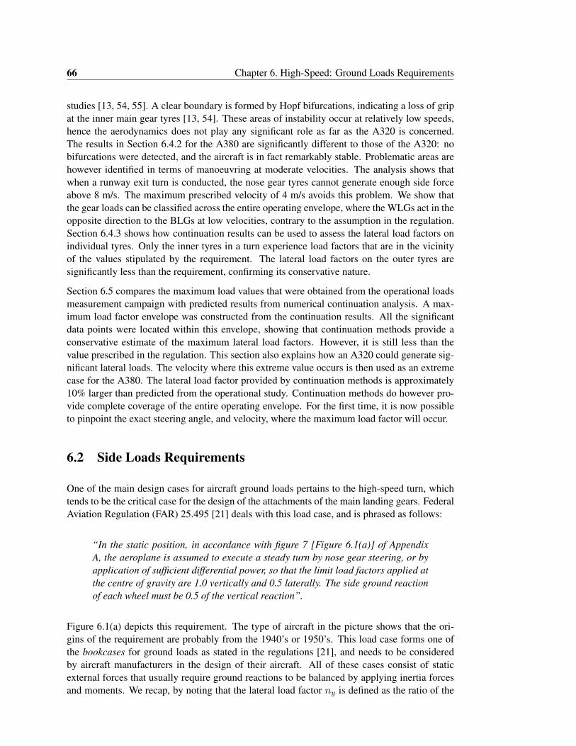
66 Chapter 6. High-Speed: Ground Loads Requirements
studies [13, 54, 55]. A clear boundary is formed by Hopf bifurcations, indicating a loss of gripat the inner main gear tyres [13, 54]. These areas of instability occur at relatively low speeds,hence the aerodynamics does not play any significant role as far as the A320 is concerned.The results in Section 6.4.2 for the A380 are significantly different to those of the A320: nobifurcations were detected, and the aircraft is in fact remarkably stable. Problematic areas arehowever identified in terms of manoeuvring at moderate velocities. The analysis shows thatwhen a runway exit turn is conducted, the nose gear tyres cannot generate enough side forceabove 8 m/s. The maximum prescribed velocity of 4 m/s avoids this problem. We show thatthe gear loads can be classified across the entire operating envelope, where the WLGs act in theopposite direction to the BLGs at low velocities, contrary to the assumption in the regulation.Section 6.4.3 shows how continuation results can be used to assess the lateral load factors onindividual tyres. Only the inner tyres in a turn experience load factors that are in the vicinityof the values stipulated by the requirement. The lateral load factors on the outer tyres aresignificantly less than the requirement, confirming its conservative nature.
Section 6.5 compares the maximum load values that were obtained from the operational loadsmeasurement campaign with predicted results from numerical continuation analysis. A max-imum load factor envelope was constructed from the continuation results. All the significantdata points were located within this envelope, showing that continuation methods provide aconservative estimate of the maximum lateral load factors. However, it is still less than thevalue prescribed in the regulation. This section also explains how an A320 could generate sig-nificant lateral loads. The velocity where this extreme value occurs is then used as an extremecase for the A380. The lateral load factor provided by continuation methods is approximately10% larger than predicted from the operational study. Continuation methods do however pro-vide complete coverage of the entire operating envelope. For the first time, it is now possibleto pinpoint the exact steering angle, and velocity, where the maximum load factor will occur.
6.2 Side Loads Requirements
One of the main design cases for aircraft ground loads pertains to the high-speed turn, whichtends to be the critical case for the design of the attachments of the main landing gears. FederalAviation Regulation (FAR) 25.495 [21] deals with this load case, and is phrased as follows:
“In the static position, in accordance with figure 7 [Figure 6.1(a)] of AppendixA, the aeroplane is assumed to execute a steady turn by nose gear steering, or byapplication of sufficient differential power, so that the limit load factors applied atthe centre of gravity are 1.0 vertically and 0.5 laterally. The side ground reactionof each wheel must be 0.5 of the vertical reaction”.
Figure 6.1(a) depicts this requirement. The type of aircraft in the picture shows that the ori-gins of the requirement are probably from the 1940’s or 1950’s. This load case forms one ofthe bookcases for ground loads as stated in the regulations [21], and needs to be consideredby aircraft manufacturers in the design of their aircraft. All of these cases consist of staticexternal forces that usually require ground reactions to be balanced by applying inertia forcesand moments. We recap, by noting that the lateral load factor ny is defined as the ratio of the
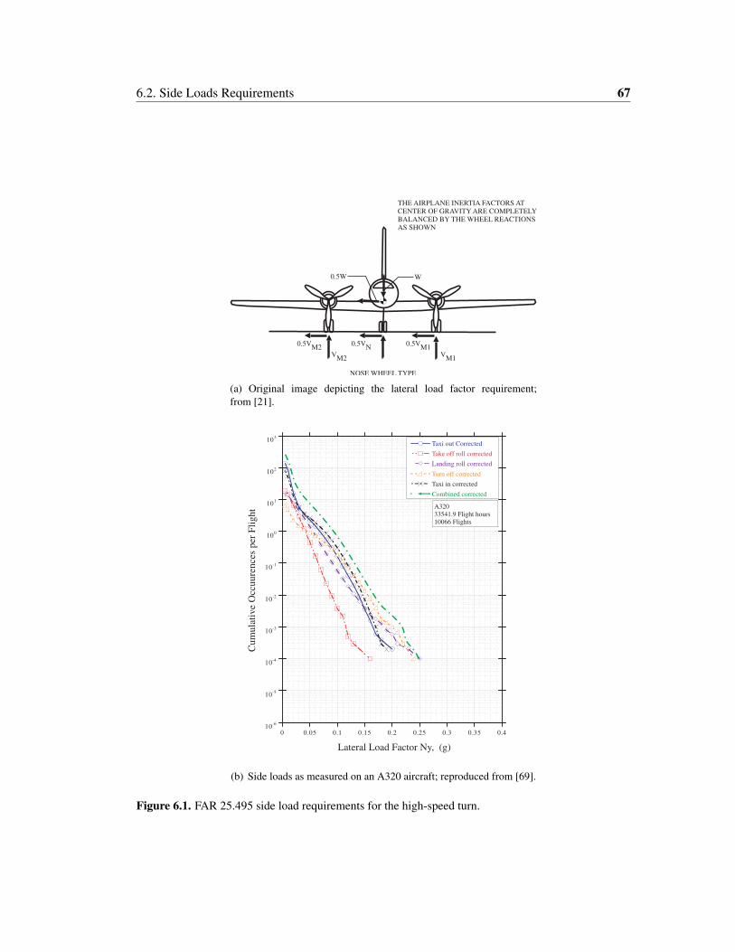
6.2. Side Loads Requirements 67
0.5VM2
0.5VN
0.5VM1
VM2
VM1
NOSE WHEEL TYPE
THE AIRPLANE INERTIA FACTORS AT
CENTER OF GRAVITY ARE COMPLETELY
BALANCED BY THE WHEEL REACTIONS
AS SHOWN
0.5W W
(a) Original image depicting the lateral load factor requirement;from [21].
10-6
10-5
10-4
10-3
10-2
10-1
100
101
102
103
0 0.05 0.1 0.15 0.2 0.25 0.3 0.35 0.4
Taxi out Corrected
Take off roll corrected
Landing roll corrected
Turn off corrected
Taxi in corrected
Combined corrected
A320
33541.9 Flight hours
10066 Flights
Cum
ula
tive
Occ
uure
nce
s per
Fli
ght
Lateral Load Factor Ny, (g)
(b) Side loads as measured on an A320 aircraft; reproduced from [69].
Figure 6.1. FAR 25.495 side load requirements for the high-speed turn.
68 Chapter 6. High-Speed: Ground Loads Requirements
lateral force over the vertical force, which is 0.5 for this specific regulation. Reference [69]states that little is known about the origin of this regulation, or even under what operationalconditions such a loading condition might occur. The regulation was clearly brought in whenaircraft were much smaller than they are nowadays, and it may be that aircraft with more thantwo main gears did not exist at the point in history when the regulation was drafted; however,we have no evidence for this assertion. Reference [69] also states that landing gear and aircraftmanufacturers believe that the current 0.5g lateral load factor requirement specified by FAR25.495 is too stringent. The regulatory authorities are however extremely reluctant to modifythis requirement in the absence of data to back such a decision. The requirement has clearlyensured safe aircraft operations, and consequently overwhelming evidence would be neededfor its relaxation.
6.2.1 Limitations of the Regulation
The loads produced by the high-speed turn form one of the limit load cases and, as such, con-tribute towards the aircraft and landing gear limit load envelopes. The loads can be calculatedaccurately for aircraft with statically determinate (tricycle) gear arrangements such as the A320,where the fuselage and gears are assumed to be rigid [54, 55]. However, statically indetermi-nate (more than three gears) arrangements such as the A380, pose computational challenges,where minimum energy techniques are needed to calculate the response of the aircraft [15].This was discussed in Section 2.3. Such an approach is needed to protect any one gear againstdisproportionate loading due to the stiffness characteristics of the gears and fuselage [74]. Forthis reason aircraft manufacturers tend to include other cases (in addition to the bookcases)into their analysis. These cases are based on years of experience that try to cover day-to-dayoperational scenarios. These additional cases are known as rational cases, as they utilise mod-els that contain a more accurate representation of the real physics and dynamics of the system.In particular, the dynamic response of the airplane is included. Structural inertia, flexibility,and damping are accounted for, as well as distributed aerodynamic lift and moments. This is amore realistic method of investigating the actual forces on the aircraft.
Dynamic calculations are employed for rational cases such as taxiing or landing, and may formpart of the limit load envelope. It is also normal practice to use such dynamic calculations toestablish the aircraft fatigue loads. Nonlinear effects within the tyres and landing gears makeit difficult to find the exact values for the steering angles and velocities where the maximumlateral loading may occur. This is the reason for adhering to the bookcase approach, with theaddition of rational cases. Nonlinear effects could for instance lead to multiple steady-states forthe same thrust and steering angle settings, when considering the high-speed turn, such that theresponse depends on the initial conditions and size of the perturbations on the system [13, 54].A large perturbation could for instance cause a “jump” to another steady-state. This type ofbehaviour is the motivation to use methods from the field of Dynamical Systems theory, toanalyse the dynamics of an aircraft on the ground [13, 15, 54, 55, 56].
6.2.2 FAA Operational Loads Study
In answer to the points mentioned in the previous section and in Reference [69], the FAA con-ducted a large operational loads testing campaign, where it aimed to identify the maximum
6.3. Aircraft Loads from the Static Balance Equations 69
operational loads that can be experienced by in-service aircraft. A critical assessment of theloads was then made against the current regulations [69]. The findings from this study showedthat it was very difficult to obtain lateral accelerations above 0.3g for any aircraft types. As anexample, Figure 6.1(b) shows the measured side loads for the A320 that was used in [69]; itshows that they did not exceed 0.25g for the approximately 10,000 flights that were recorded.The authors of [69] collated the information for all the assessed aircraft and derived an empiri-cal formula to predict the likelihood of obtaining a certain g-level in 1000 flights as
N = N0e−lsnlmn2
y . (6.1)
Here N is the number of cumulative occurrences of any lateral load factor ny in 1000 flights,where ny is the maximum lateral load factor measured during a turn; ln represents the wheelbase and lm the track width. N0 is the number of cumulative occurrences at ny = 0; s rep-resents a shape parameter specific to the aircraft being studied. Each aircraft therefore hasits own factor for N0 and s, that are derived from the study. The authors of [69] average thefactors of all the aircraft to obtain a generic formula that can be used for any aircraft. Theirinitial assessments show that the taxi-in phase seems to generate larger load factors, but theypoint out that corrections need to be made to the taxi-in data, due to the fuel that is burnedbetween the maximum ramp weight (MRW) and maximum landing weight (MLW) condition.Nonetheless, the taxi-in phase still seems to be more critical, even after such corrections aremade. The generic formula to obtain the lateral load factor for the taxi-in phase then becomes
N = 2225.7e−l0.498n lmn2
y . (6.2)
This equation can be rearranged to obtain the lateral load factor as a function of the layout of thegears, and the probability of an occurrence of the obtained factor in 1000 flights. If we assumethat the life of an aircraft is no more than 100,000 flights, then the value of N becomes 0.01.Figure 6.2(a) contains a contour map of the maximum lateral load factor that can be expected atleast once in 100,000 flights, for different track width and wheel base combinations. Existingaircraft are overlaid onto the contour map, which shows that smaller aircraft experience higherlateral load factors than larger aircraft. This maximum value is still significantly lower thanthe 0.5g specified by the regulation. It can be seen that a maximum value of 0.28g is predictedfor the A320, which has never been measured in the tests (see Figure 6.1(b)), and a value ofbetween 0.16 and 0.17 is predicted for the A380.
The authors of [69] then insert the dimensions of the Boeing 737-400 into this equation, andcalculate the probability of experiencing a 0.5g lateral load factor. This probability is usedas a baseline for a comparison with other aircraft. Equation (6.2) is then used to obtain themaximum lateral expected load. Figure 6.2(b) shows the results from this study [69]. It isapparent from both parts of Figure 6.2 that the gear positioning and size of the aircraft have amajor influence on the lateral load factor that can be achieved. This information can now beused by the FAA for future considerations pertaining to the regulation.
6.3 Aircraft Loads from the Static Balance Equations
The high-speed turn regulation is interpreted by aircraft manufacturers to require the aircraft toconduct a turn by using nose wheel steering or differential power. A lateral acceleration of 0.5g
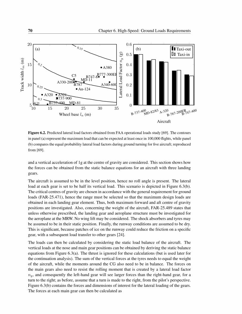
70 Chapter 6. High-Speed: Ground Loads Requirements
10 15 20 25 30 355
10
15
200.15
0.2
0.25
0.30.35
(a)
A320 A321
A330-200A340-600
A380
An-124
C5
B737-400B737-900
B747-8B777-300ER
B787
MD-81
MD-11
Wheel base ln (m)
Trac
kw
idthl m
(m)
B-737-400MD-82/83 A-320
B-767-200ERB-747-400
0
0.1
0.2
0.3
0.4
0.5
0.6(b)
AircraftL
ater
alL
oad
Fact
orny
(g)
Taxi-outTaxi-in
Figure 6.2. Predicted lateral load factors obtained from FAA operational loads study [69]. The contoursin panel (a) represent the maximum load that can be expected at least once in 100,000 flights, while panel(b) compares the equal probability lateral load factors during ground turning for five aircraft; reproducedfrom [69].
and a vertical acceleration of 1g at the centre of gravity are considered. This section shows howthe forces can be obtained from the static balance equations for an aircraft with three landinggears.
The aircraft is assumed to be in the level position, hence no roll angle is present. The lateralload at each gear is set to be half its vertical load. This scenario is depicted in Figure 6.3(b).The critical centres of gravity are chosen in accordance with the general requirement for groundloads (FAR-25.471), hence the range must be selected so that the maximum design loads areobtained in each landing gear element. Thus, both maximum forward and aft centre of gravitypositions are investigated. Also, concerning the weight of the aircraft, FAR-25.489 states thatunless otherwise prescribed, the landing gear and aeroplane structure must be investigated forthe aeroplane at the MRW. No wing lift may be considered. The shock absorbers and tyres maybe assumed to be in their static position. Finally, the runway conditions are assumed to be dry.This is significant, because patches of ice on the runway could reduce the friction on a specificgear, with a subsequent load transfer to other gears [24].
The loads can then be calculated by considering the static load balance of the aircraft. Thevertical loads at the nose and main gear positions can be obtained by deriving the static balanceequations from Figure 6.3(a). The thrust is ignored for these calculations (but is used later forthe continuation analysis). The sum of the vertical forces at the tyres needs to equal the weightof the aircraft, while the moments around the CG also need to be in balance. The forces onthe main gears also need to resist the rolling moment that is created by a lateral load factorny, and consequently the left-hand gear will see larger forces than the right-hand gear, for aturn to the right; as before, assume that a turn is made to the right, from the pilot’s perspective.Figure 6.3(b) contains the forces and dimensions of interest for the lateral loading of the gears.The forces at each main gear can then be calculated as
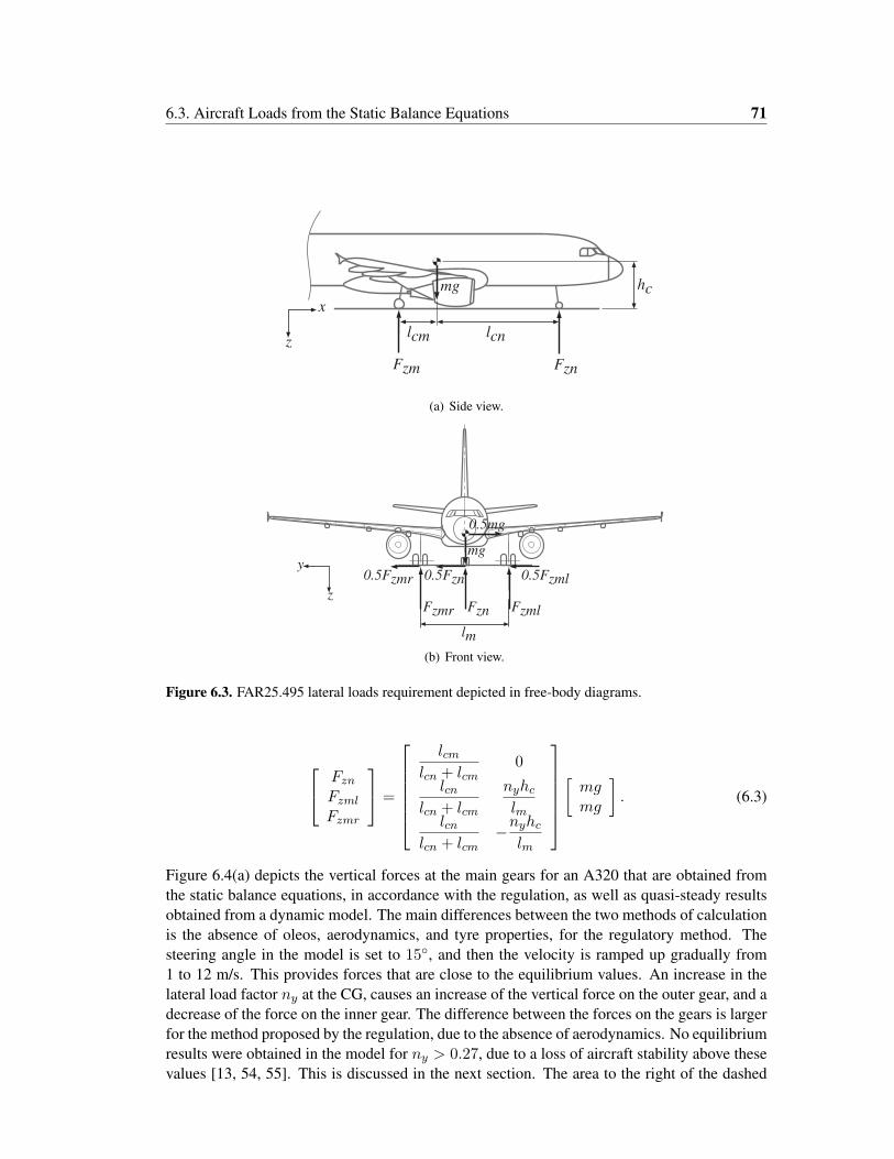
6.3. Aircraft Loads from the Static Balance Equations 71
Fzm Fzn
mg
lcnlcm
hc
z
x
(a) Side view.
Fzmr FzmlFzn
0.5Fzmr 0.5Fzml0.5Fzn
mg
0.5mg
lm
z
y
(b) Front view.
Figure 6.3. FAR25.495 lateral loads requirement depicted in free-body diagrams.
FznFzmlFzmr
=
lcm
lcn + lcm0
lcnlcn + lcm
nyhclm
lcnlcn + lcm
−nyhclm
[mgmg
]. (6.3)
Figure 6.4(a) depicts the vertical forces at the main gears for an A320 that are obtained fromthe static balance equations, in accordance with the regulation, as well as quasi-steady resultsobtained from a dynamic model. The main differences between the two methods of calculationis the absence of oleos, aerodynamics, and tyre properties, for the regulatory method. Thesteering angle in the model is set to 15◦, and then the velocity is ramped up gradually from1 to 12 m/s. This provides forces that are close to the equilibrium values. An increase in thelateral load factor ny at the CG, causes an increase of the vertical force on the outer gear, and adecrease of the force on the inner gear. The difference between the forces on the gears is largerfor the method proposed by the regulation, due to the absence of aerodynamics. No equilibriumresults were obtained in the model for ny > 0.27, due to a loss of aircraft stability above thesevalues [13, 54, 55]. This is discussed in the next section. The area to the right of the dashed
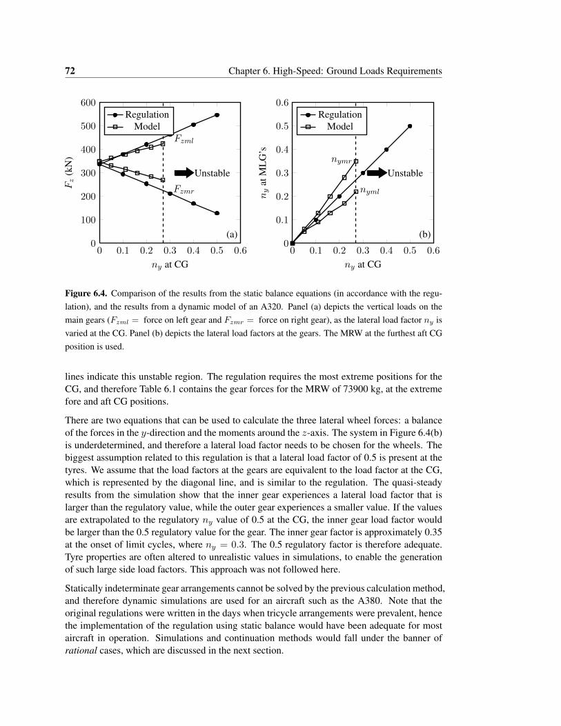
72 Chapter 6. High-Speed: Ground Loads Requirements
0 0.1 0.2 0.3 0.4 0.5 0.60
100
200
300
400
500
600
Unstable
Fzml
Fzmr
(a)
ny at CG
Fz
(kN
)
RegulationModel
0 0.1 0.2 0.3 0.4 0.5 0.60
0.1
0.2
0.3
0.4
0.5
0.6
Unstable
nyml
nymr
(b)
ny at CGny
atM
LG
’s
RegulationModel
Figure 6.4. Comparison of the results from the static balance equations (in accordance with the regu-lation), and the results from a dynamic model of an A320. Panel (a) depicts the vertical loads on themain gears (Fzml = force on left gear and Fzmr = force on right gear), as the lateral load factor ny isvaried at the CG. Panel (b) depicts the lateral load factors at the gears. The MRW at the furthest aft CGposition is used.
lines indicate this unstable region. The regulation requires the most extreme positions for theCG, and therefore Table 6.1 contains the gear forces for the MRW of 73900 kg, at the extremefore and aft CG positions.
There are two equations that can be used to calculate the three lateral wheel forces: a balanceof the forces in the y-direction and the moments around the z-axis. The system in Figure 6.4(b)is underdetermined, and therefore a lateral load factor needs to be chosen for the wheels. Thebiggest assumption related to this regulation is that a lateral load factor of 0.5 is present at thetyres. We assume that the load factors at the gears are equivalent to the load factor at the CG,which is represented by the diagonal line, and is similar to the regulation. The quasi-steadyresults from the simulation show that the inner gear experiences a lateral load factor that islarger than the regulatory value, while the outer gear experiences a smaller value. If the valuesare extrapolated to the regulatory ny value of 0.5 at the CG, the inner gear load factor wouldbe larger than the 0.5 regulatory value for the gear. The inner gear factor is approximately 0.35at the onset of limit cycles, where ny = 0.3. The 0.5 regulatory factor is therefore adequate.Tyre properties are often altered to unrealistic values in simulations, to enable the generationof such large side load factors. This approach was not followed here.
Statically indeterminate gear arrangements cannot be solved by the previous calculation method,and therefore dynamic simulations are used for an aircraft such as the A380. Note that theoriginal regulations were written in the days when tricycle arrangements were prevalent, hencethe implementation of the regulation using static balance would have been adequate for mostaircraft in operation. Simulations and continuation methods would fall under the banner ofrational cases, which are discussed in the next section.
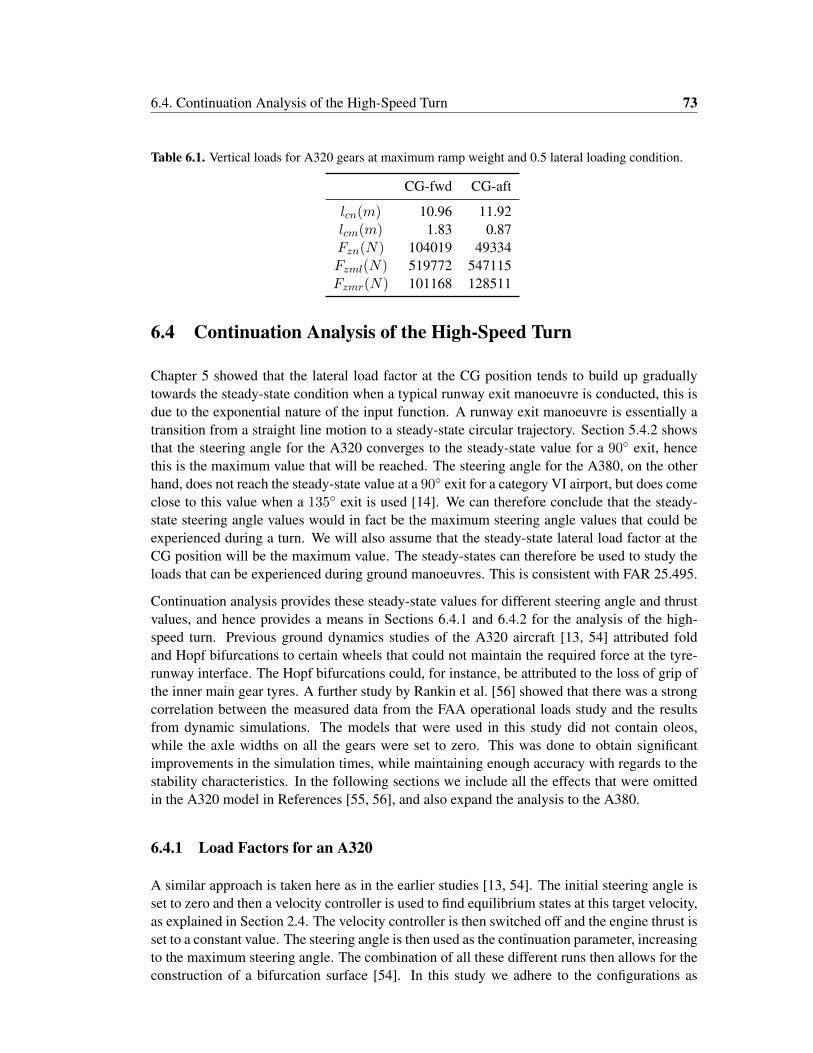
6.4. Continuation Analysis of the High-Speed Turn 73
Table 6.1. Vertical loads for A320 gears at maximum ramp weight and 0.5 lateral loading condition.
CG-fwd CG-aft
lcn(m) 10.96 11.92lcm(m) 1.83 0.87Fzn(N) 104019 49334Fzml(N) 519772 547115Fzmr(N) 101168 128511
6.4 Continuation Analysis of the High-Speed Turn
Chapter 5 showed that the lateral load factor at the CG position tends to build up graduallytowards the steady-state condition when a typical runway exit manoeuvre is conducted, this isdue to the exponential nature of the input function. A runway exit manoeuvre is essentially atransition from a straight line motion to a steady-state circular trajectory. Section 5.4.2 showsthat the steering angle for the A320 converges to the steady-state value for a 90◦ exit, hencethis is the maximum value that will be reached. The steering angle for the A380, on the otherhand, does not reach the steady-state value at a 90◦ exit for a category VI airport, but does comeclose to this value when a 135◦ exit is used [14]. We can therefore conclude that the steady-state steering angle values would in fact be the maximum steering angle values that could beexperienced during a turn. We will also assume that the steady-state lateral load factor at theCG position will be the maximum value. The steady-states can therefore be used to study theloads that can be experienced during ground manoeuvres. This is consistent with FAR 25.495.
Continuation analysis provides these steady-state values for different steering angle and thrustvalues, and hence provides a means in Sections 6.4.1 and 6.4.2 for the analysis of the high-speed turn. Previous ground dynamics studies of the A320 aircraft [13, 54] attributed foldand Hopf bifurcations to certain wheels that could not maintain the required force at the tyre-runway interface. The Hopf bifurcations could, for instance, be attributed to the loss of grip ofthe inner main gear tyres. A further study by Rankin et al. [56] showed that there was a strongcorrelation between the measured data from the FAA operational loads study and the resultsfrom dynamic simulations. The models that were used in this study did not contain oleos,while the axle widths on all the gears were set to zero. This was done to obtain significantimprovements in the simulation times, while maintaining enough accuracy with regards to thestability characteristics. In the following sections we include all the effects that were omittedin the A320 model in References [55, 56], and also expand the analysis to the A380.
6.4.1 Load Factors for an A320
A similar approach is taken here as in the earlier studies [13, 54]. The initial steering angle isset to zero and then a velocity controller is used to find equilibrium states at this target velocity,as explained in Section 2.4. The velocity controller is then switched off and the engine thrust isset to a constant value. The steering angle is then used as the continuation parameter, increasingto the maximum steering angle. The combination of all these different runs then allows for theconstruction of a bifurcation surface [54]. In this study we adhere to the configurations as
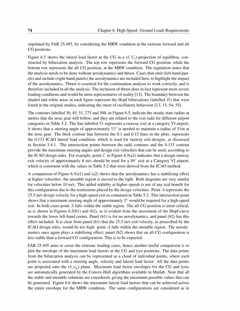
74 Chapter 6. High-Speed: Ground Loads Requirements
stipulated by FAR 25.495, by considering the MRW condition at the extreme forward and aftCG positions.
Figure 6.5 shows the lateral load factor at the CG in a (δ, Vn)-projection of equilibria, con-structed by bifurcation analysis. The top row represents the forward CG position, while thebottom row represents the aft CG position, at the MRW condition. The regulation states thatthe analysis needs to be done without aerodynamics and thrust. Cases that omit (left-hand pan-els) and include (right-hand panels) the aerodynamics are included here, to highlight the impactof the aerodynamics. Thrust is essential for the continuation analysis to work correctly, and istherefore included in all the analysis. The inclusion of thrust does in fact represent more severeloading conditions and would be more representative of reality [13]. The boundary between theshaded and white areas in each figure represent the Hopf bifurcations (labelled H) that werefound in the original studies, indicating the onset of oscillatory behaviour [13, 15, 54, 55].
The contours labelled 30, 45, 51, 275 and 500, in Figure 6.5, indicate the steady-state radius inmetres that the nose gear will follow, and they are related to the exit radii for different airportcategories in Table 5.2. The line labelled 51 represents a runway exit at a category VI airport;it shows that a steering angle of approximately 15◦ is needed to maintain a radius of 51m atthe nose gear. The thick contour line between the 0.1 and 0.15 lines in the plots, representsthe 0.133 ICAO lateral load condition, which is used for runway exit designs, as discussedin Section 5.4.1. The intersection points between the radii contours and the 0.133 contourprovide the maximum steering angles and design exit velocities that can be used, according tothe ICAO design rules. For example, point C in Figure 6.5(a2) indicates that a design runwayexit velocity of approximately 8 m/s should be used for a 90◦ exit at a Category VI airport,which is consistent with the values in Table 5.2 that were derived from the ICAO method.
A comparison of Figure 6.5(a1) and (a2) shows that the aerodynamics has a stabilising effectat higher velocities: the unstable region is moved to the right. Both diagrams are very similarfor velocities below 10 m/s. This added stability at higher speeds is not of any real benefit forthis configuration due to the restrictions placed by the design velocities. Point A represents the25.5 m/s design velocity for a high-speed exit as contained in Table 5.2. This intersection pointshows that a maximum steering angle of approximately 2◦ would be required for a high-speedexit. In both cases point A falls within the stable region. The aft CG position is more critical,as is shown in Figures 6.5(b1) and (b2), as is evident from the movement of the Hopf-curvetowards the lower left-hand corner. Panel (b1) is for no aerodynamics, and panel (b2) has thiseffect included. It is clear from panel (b1) that the 25.5 m/s exit velocity, as prescribed by theICAO design rules, would be too high: point A falls within the unstable region. The aerody-namics once again plays a stabilising effect; panel (b2) shows that an aft CG configuration isless stable than a forward CG configuration. This is to be expected.
FAR 25.495 aims to cover the extreme loading cases, hence another useful comparison is toplot the envelope of the maximum load factors at the CG and tyre positions. The data pointsfrom the bifurcation analysis can be represented as a cloud of individual points, where eachpoint is associated with a steering angle, velocity and lateral load factor. All the data pointsare projected onto the (δ, ny) plane. Maximum load factor envelopes for the CG and tyresare automatically generated by the Convex-Hull algorithms available in Matlab. Note that allthe stable and unstable solutions are considered, giving the maximum possible values that canbe generated. Figure 6.6 shows the maximum lateral load factors that can be achieved acrossthe entire envelope for the MRW condition. The same configurations are considered as in
6.4. Continuation Analysis of the High-Speed Turn 75
0.1 0.2 0.25
0 5 10 15 20 25 30 35
35
30
25
20
15
10
5
0
0.150.3
Unstable
(a1)
0.1 0.2 0.250.15 0.3
(a2)
5 10 15 20 25 30 35
35
30
25
20
15
10
5
00
Unstable
30
45
51
275
500
0.1 0.2 0.250.15
(b1)
0 5 10 15 20 25 30 35
35
30
25
20
15
10
5
0
Unstable
0.1 0.2 0.25
0.15
(b2)
5 10 15 20 25 30 35
35
30
25
20
15
10
5
0
Unstable
0
30
45
51
275
500
30
45
51
275
500
30
45
51
275
500
0.133
0.133
0.133
0.133
A
AA
H H
HH
Aero: OffCG: Forward
Aero: OnCG: Forward
Aero: OnCG: Aft
Aero: OffCG: Aft
Vn
(m/s
)
δ (deg)
Vn
(m/s
)
δ (deg)
A
D
C
B
B
Figure 6.5. Lateral load factor contours at the CG for the A320 at the MRW, obtained from bifurcationanalysis. The onset of instability is characterised by limit point and Hopf bifurcations. Panel (a1) isfor forward CG position without aerodynamics; Panel (a2) is for the same configuration with aerody-namics included. Panel (b1) is with an aft CG position; panel (b2) is for the same configuration withaerodynamics included. The behaviour at points A, B, C and D are compared.
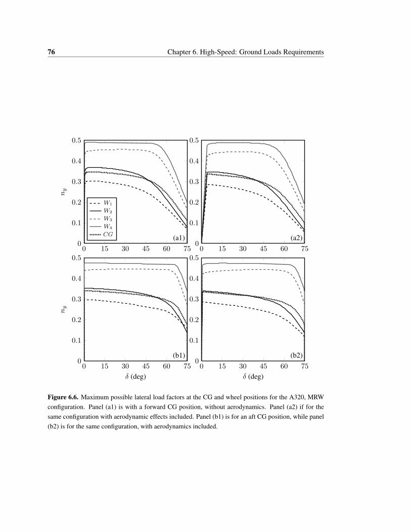
76 Chapter 6. High-Speed: Ground Loads Requirements
0 15 30 45 60 750
0.1
0.2
0.3
0.4
0.5
(a1)
ny
W1
W2
W3
W4
CG
0 15 30 45 60 750
0.1
0.2
0.3
0.4
0.5
(a2)
0 15 30 45 60 750
0.1
0.2
0.3
0.4
0.5
(b1)
δ (deg)
ny
0 15 30 45 60 750
0.1
0.2
0.3
0.4
0.5
(b2)
δ (deg)
Figure 6.6. Maximum possible lateral load factors at the CG and wheel positions for the A320, MRWconfiguration. Panel (a1) is with a forward CG position, without aerodynamics. Panel (a2) if for thesame configuration with aerodynamic effects included. Panel (b1) is for an aft CG position, while panel(b2) is for the same configuration, with aerodynamics included.
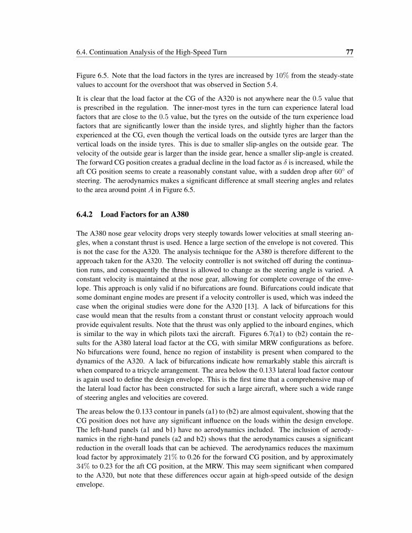
6.4. Continuation Analysis of the High-Speed Turn 77
Figure 6.5. Note that the load factors in the tyres are increased by 10% from the steady-statevalues to account for the overshoot that was observed in Section 5.4.
It is clear that the load factor at the CG of the A320 is not anywhere near the 0.5 value thatis prescribed in the regulation. The inner-most tyres in the turn can experience lateral loadfactors that are close to the 0.5 value, but the tyres on the outside of the turn experience loadfactors that are significantly lower than the inside tyres, and slightly higher than the factorsexperienced at the CG, even though the vertical loads on the outside tyres are larger than thevertical loads on the inside tyres. This is due to smaller slip-angles on the outside gear. Thevelocity of the outside gear is larger than the inside gear, hence a smaller slip-angle is created.The forward CG position creates a gradual decline in the load factor as δ is increased, while theaft CG position seems to create a reasonably constant value, with a sudden drop after 60◦ ofsteering. The aerodynamics makes a significant difference at small steering angles and relatesto the area around point A in Figure 6.5.
6.4.2 Load Factors for an A380
The A380 nose gear velocity drops very steeply towards lower velocities at small steering an-gles, when a constant thrust is used. Hence a large section of the envelope is not covered. Thisis not the case for the A320. The analysis technique for the A380 is therefore different to theapproach taken for the A320. The velocity controller is not switched off during the continua-tion runs, and consequently the thrust is allowed to change as the steering angle is varied. Aconstant velocity is maintained at the nose gear, allowing for complete coverage of the enve-lope. This approach is only valid if no bifurcations are found. Bifurcations could indicate thatsome dominant engine modes are present if a velocity controller is used, which was indeed thecase when the original studies were done for the A320 [13]. A lack of bifurcations for thiscase would mean that the results from a constant thrust or constant velocity approach wouldprovide equivalent results. Note that the thrust was only applied to the inboard engines, whichis similar to the way in which pilots taxi the aircraft. Figures 6.7(a1) to (b2) contain the re-sults for the A380 lateral load factor at the CG, with similar MRW configurations as before.No bifurcations were found, hence no region of instability is present when compared to thedynamics of the A320. A lack of bifurcations indicate how remarkably stable this aircraft iswhen compared to a tricycle arrangement. The area below the 0.133 lateral load factor contouris again used to define the design envelope. This is the first time that a comprehensive map ofthe lateral load factor has been constructed for such a large aircraft, where such a wide rangeof steering angles and velocities are covered.
The areas below the 0.133 contour in panels (a1) to (b2) are almost equivalent, showing that theCG position does not have any significant influence on the loads within the design envelope.The left-hand panels (a1 and b1) have no aerodynamics included. The inclusion of aerody-namics in the right-hand panels (a2 and b2) shows that the aerodynamics causes a significantreduction in the overall loads that can be achieved. The aerodynamics reduces the maximumload factor by approximately 21% to 0.26 for the forward CG position, and by approximately34% to 0.23 for the aft CG position, at the MRW. This may seem significant when comparedto the A320, but note that these differences occur again at high-speed outside of the designenvelope.
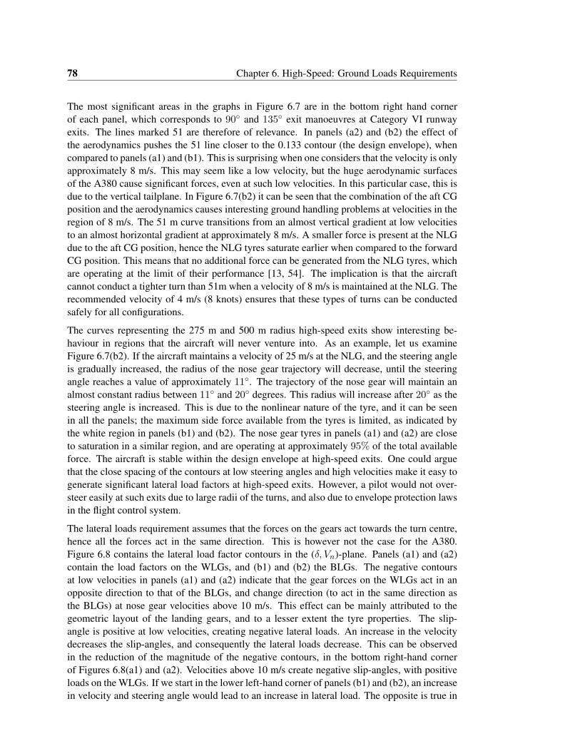
78 Chapter 6. High-Speed: Ground Loads Requirements
The most significant areas in the graphs in Figure 6.7 are in the bottom right hand cornerof each panel, which corresponds to 90◦ and 135◦ exit manoeuvres at Category VI runwayexits. The lines marked 51 are therefore of relevance. In panels (a2) and (b2) the effect ofthe aerodynamics pushes the 51 line closer to the 0.133 contour (the design envelope), whencompared to panels (a1) and (b1). This is surprising when one considers that the velocity is onlyapproximately 8 m/s. This may seem like a low velocity, but the huge aerodynamic surfacesof the A380 cause significant forces, even at such low velocities. In this particular case, this isdue to the vertical tailplane. In Figure 6.7(b2) it can be seen that the combination of the aft CGposition and the aerodynamics causes interesting ground handling problems at velocities in theregion of 8 m/s. The 51 m curve transitions from an almost vertical gradient at low velocitiesto an almost horizontal gradient at approximately 8 m/s. A smaller force is present at the NLGdue to the aft CG position, hence the NLG tyres saturate earlier when compared to the forwardCG position. This means that no additional force can be generated from the NLG tyres, whichare operating at the limit of their performance [13, 54]. The implication is that the aircraftcannot conduct a tighter turn than 51m when a velocity of 8 m/s is maintained at the NLG. Therecommended velocity of 4 m/s (8 knots) ensures that these types of turns can be conductedsafely for all configurations.
The curves representing the 275 m and 500 m radius high-speed exits show interesting be-haviour in regions that the aircraft will never venture into. As an example, let us examineFigure 6.7(b2). If the aircraft maintains a velocity of 25 m/s at the NLG, and the steering angleis gradually increased, the radius of the nose gear trajectory will decrease, until the steeringangle reaches a value of approximately 11◦. The trajectory of the nose gear will maintain analmost constant radius between 11◦ and 20◦ degrees. This radius will increase after 20◦ as thesteering angle is increased. This is due to the nonlinear nature of the tyre, and it can be seenin all the panels; the maximum side force available from the tyres is limited, as indicated bythe white region in panels (b1) and (b2). The nose gear tyres in panels (a1) and (a2) are closeto saturation in a similar region, and are operating at approximately 95% of the total availableforce. The aircraft is stable within the design envelope at high-speed exits. One could arguethat the close spacing of the contours at low steering angles and high velocities make it easy togenerate significant lateral load factors at high-speed exits. However, a pilot would not over-steer easily at such exits due to large radii of the turns, and also due to envelope protection lawsin the flight control system.
The lateral loads requirement assumes that the forces on the gears act towards the turn centre,hence all the forces act in the same direction. This is however not the case for the A380.Figure 6.8 contains the lateral load factor contours in the (δ, Vn)-plane. Panels (a1) and (a2)contain the load factors on the WLGs, and (b1) and (b2) the BLGs. The negative contoursat low velocities in panels (a1) and (a2) indicate that the gear forces on the WLGs act in anopposite direction to that of the BLGs, and change direction (to act in the same direction asthe BLGs) at nose gear velocities above 10 m/s. This effect can be mainly attributed to thegeometric layout of the landing gears, and to a lesser extent the tyre properties. The slip-angle is positive at low velocities, creating negative lateral loads. An increase in the velocitydecreases the slip-angles, and consequently the lateral loads decrease. This can be observedin the reduction of the magnitude of the negative contours, in the bottom right-hand cornerof Figures 6.8(a1) and (a2). Velocities above 10 m/s create negative slip-angles, with positiveloads on the WLGs. If we start in the lower left-hand corner of panels (b1) and (b2), an increasein velocity and steering angle would lead to an increase in lateral load. The opposite is true in
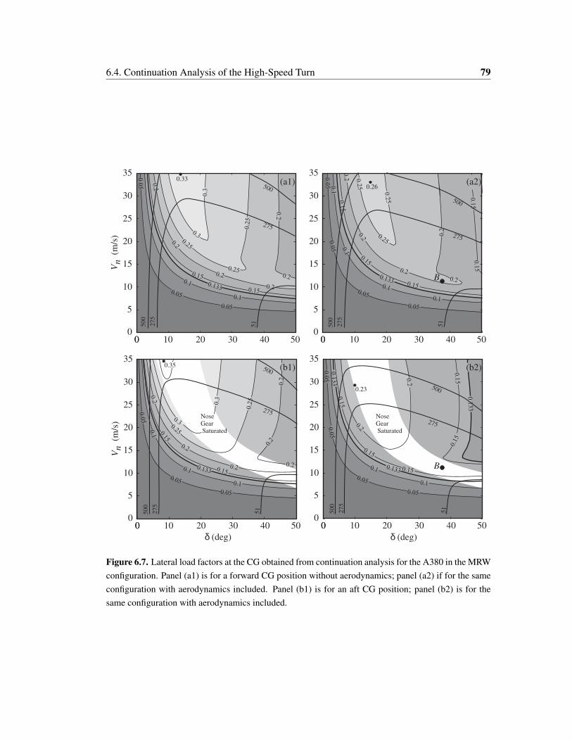
6.4. Continuation Analysis of the High-Speed Turn 79
51
275
500
35
30
25
20
15
10
5
0 10 20 300
0 40 50
(b2)
δ (deg)
51
275
500
35
30
25
20
15
10
5
Vn
(m/s
)
0 10 20 300
0 40 50
(b1)
δ (deg)
0.26
51
275
500
(a2)35
30
25
20
15
10
5
0 10 20 300
0 40 50
(a1)35
30
25
20
15
10
5
Vn
(m/s
)
0 10 20 300
0 40 50
0.33
275
500
51
500
275
500
275
500
275
500
275
NoseGearSaturated
NoseGearSaturated
0.23
0.35
NoseGearSaturated
B
B
Figure 6.7. Lateral load factors at the CG obtained from continuation analysis for the A380 in the MRWconfiguration. Panel (a1) is for a forward CG position without aerodynamics; panel (a2) if for the sameconfiguration with aerodynamics included. Panel (b1) is for an aft CG position; panel (b2) is for thesame configuration with aerodynamics included.
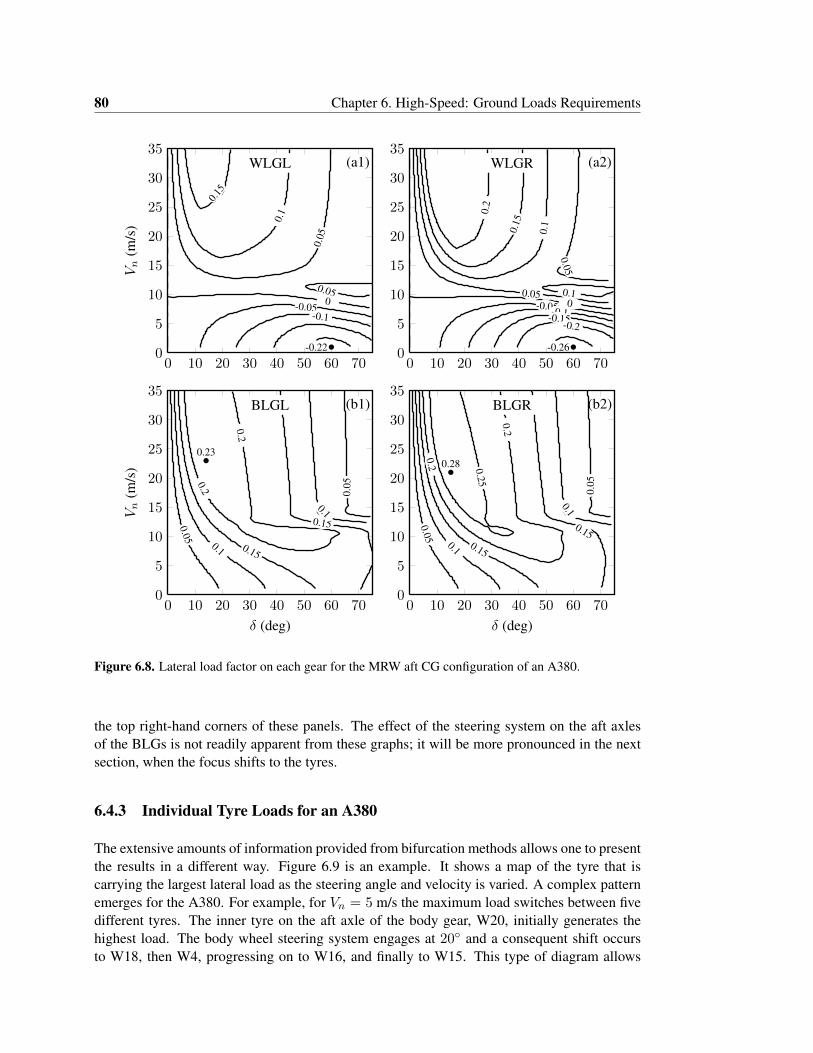
80 Chapter 6. High-Speed: Ground Loads Requirements
0 10 20 30 40 50 60 700
5
10
15
20
25
30
35
-0.22
0.15
0.1
0.05
0.05
0-0.05-0.1
(a1)WLGL
Vn
(m/s
)
0 10 20 30 40 50 60 700
5
10
15
20
25
30
35
-0.26
0.2
0.15
0.1
0.1
0.05
0.050-0.05-0.1-0.15-0.2
(a2)WLGR
0 10 20 30 40 50 60 700
5
10
15
20
25
30
35
0.23
0.2
0.2
0.15
0.15
0.1
0.1
0.05
0.05
(b1)BLGL
δ (deg)
Vn
(m/s
)
0 10 20 30 40 50 60 700
5
10
15
20
25
30
35
0.28 0.25
0.2
0.2
0.150.15
0.1
0.1
0.05
0.05
(b2)BLGR
δ (deg)
Figure 6.8. Lateral load factor on each gear for the MRW aft CG configuration of an A380.
the top right-hand corners of these panels. The effect of the steering system on the aft axlesof the BLGs is not readily apparent from these graphs; it will be more pronounced in the nextsection, when the focus shifts to the tyres.
6.4.3 Individual Tyre Loads for an A380
The extensive amounts of information provided from bifurcation methods allows one to presentthe results in a different way. Figure 6.9 is an example. It shows a map of the tyre that iscarrying the largest lateral load as the steering angle and velocity is varied. A complex patternemerges for the A380. For example, for Vn = 5 m/s the maximum load switches between fivedifferent tyres. The inner tyre on the aft axle of the body gear, W20, initially generates thehighest load. The body wheel steering system engages at 20◦ and a consequent shift occursto W18, then W4, progressing on to W16, and finally to W15. This type of diagram allows
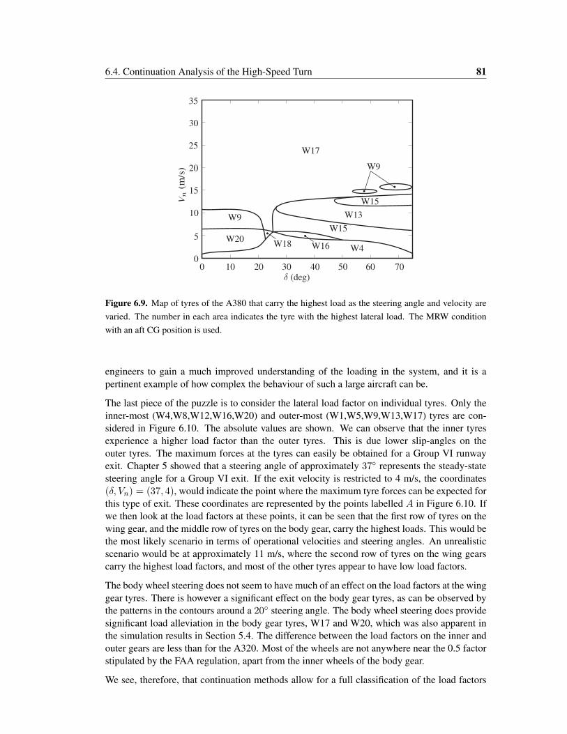
6.4. Continuation Analysis of the High-Speed Turn 81
0 10 20 30 40 50 60 700
5
10
15
20
25
30
35
Vn
(m/s
)
δ (deg)
W20
W9
W4W18 W16
W15W13
W9
W15
W17
Figure 6.9. Map of tyres of the A380 that carry the highest load as the steering angle and velocity arevaried. The number in each area indicates the tyre with the highest lateral load. The MRW conditionwith an aft CG position is used.
engineers to gain a much improved understanding of the loading in the system, and it is apertinent example of how complex the behaviour of such a large aircraft can be.
The last piece of the puzzle is to consider the lateral load factor on individual tyres. Only theinner-most (W4,W8,W12,W16,W20) and outer-most (W1,W5,W9,W13,W17) tyres are con-sidered in Figure 6.10. The absolute values are shown. We can observe that the inner tyresexperience a higher load factor than the outer tyres. This is due lower slip-angles on theouter tyres. The maximum forces at the tyres can easily be obtained for a Group VI runwayexit. Chapter 5 showed that a steering angle of approximately 37◦ represents the steady-statesteering angle for a Group VI exit. If the exit velocity is restricted to 4 m/s, the coordinates(δ, Vn) = (37, 4), would indicate the point where the maximum tyre forces can be expected forthis type of exit. These coordinates are represented by the points labelled A in Figure 6.10. Ifwe then look at the load factors at these points, it can be seen that the first row of tyres on thewing gear, and the middle row of tyres on the body gear, carry the highest loads. This would bethe most likely scenario in terms of operational velocities and steering angles. An unrealisticscenario would be at approximately 11 m/s, where the second row of tyres on the wing gearscarry the highest load factors, and most of the other tyres appear to have low load factors.
The body wheel steering does not seem to have much of an effect on the load factors at the winggear tyres. There is however a significant effect on the body gear tyres, as can be observed bythe patterns in the contours around a 20◦ steering angle. The body wheel steering does providesignificant load alleviation in the body gear tyres, W17 and W20, which was also apparent inthe simulation results in Section 5.4. The difference between the load factors on the inner andouter gears are less than for the A320. Most of the wheels are not anywhere near the 0.5 factorstipulated by the FAA regulation, apart from the inner wheels of the body gear.
We see, therefore, that continuation methods allow for a full classification of the load factors
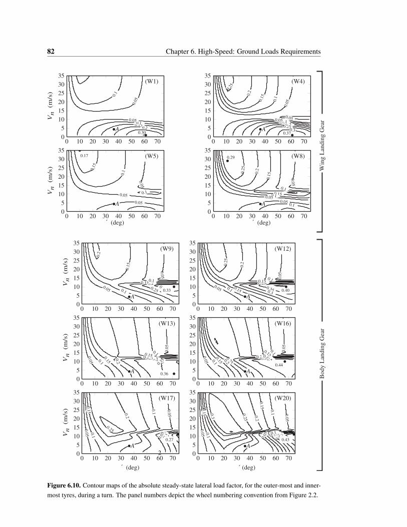
82 Chapter 6. High-Speed: Ground Loads Requirements
0 10 20 30 40 50 60 700
5
10
15
20
25
30
35
0.20.150.1
0.1
0.05
0.05
0.30
(W1)
0 10 20 30 40 50 60 700
5
10
15
20
25
30
35
0.25
0.25
0.2
0.2
0.15
0.1
5
0.1
0.1
0.050.05
0.0
5
0.37
(W4)
0 10 20 30 40 50 60 700
5
10
15
20
25
30
35
0.15
0.1
0.1
0.0
5
0.05
0.05
0.17 (W5)
0 10 20 30 40 50 60 700
5
10
15
20
25
30
35
0.2
5
0.2
0.15
0.1
5
0.1
0.1
0.1
0.0
5
0.05
0.05
0.29 (W8)
0 10 20 30 40 50 60 700
5
10
15
20
25
30
35
0.30.25
0.2
0.2
0.15
0.1
5
0.1
0.1
0.0
5
0.05 0.33
(W9)
0 10 20 30 40 50 60 700
5
10
15
20
25
30
35
0.350.3
0.25
0.2
5
0.2
0.2
0.15
0.15
0.1
0.1
0.0
5
0.05 0.40
(W12)
0 10 20 30 40 50 60 700
5
10
15
20
25
30
35
0.35
0.30.250.20.2
0.150.15
0.1
0.1
0.0
5
0.0
5
0.36
(W13)
0 10 20 30 40 50 60 700
5
10
15
20
25
30
35
0.40.350.30.250.25
0.2
0.2
0.15
0.15
0.1
0.1
0.0
5
0.0
5
0.44
(W16)
0 10 20 30 40 50 60 700
5
10
15
20
25
30
35
0.25
0.2
0.1
5
0.1
0.1
0.1
0.05
0.0
5
0.0
5
0.27
(W17)
(deg)
0 10 20 30 40 50 60 700
5
10
15
20
25
30
35
0.3
0.3
0.2
5
0.2
5
0.2
0.2
0.15
0.1
50.1
5
0.1
0.1
0.1
0.0
5
0.05
0.0
5
0.43
(W20)
(deg)
2
(deg) (deg)
Body L
andin
g G
ear
Win
g L
andin
g G
ear
´´
´ ´
Vn
(m/s
)V
n(m
/s)
Vn
(m/s
)V
n(m
/s)
Vn
(m/s
)
A A
A A
A A
AA
A A
0.3
Figure 6.10. Contour maps of the absolute steady-state lateral load factor, for the outer-most and inner-most tyres, during a turn. The panel numbers depict the wheel numbering convention from Figure 2.2.
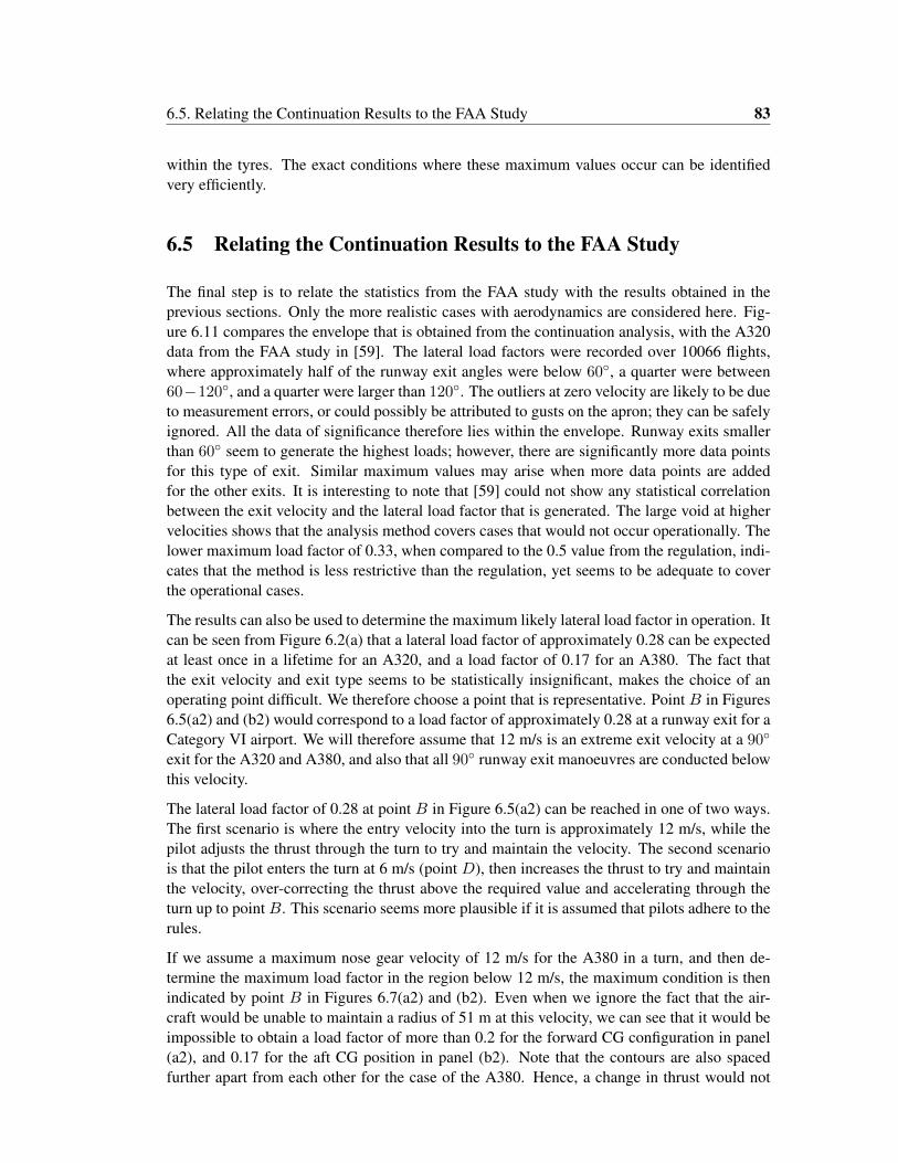
6.5. Relating the Continuation Results to the FAA Study 83
within the tyres. The exact conditions where these maximum values occur can be identifiedvery efficiently.
6.5 Relating the Continuation Results to the FAA Study
The final step is to relate the statistics from the FAA study with the results obtained in theprevious sections. Only the more realistic cases with aerodynamics are considered here. Fig-ure 6.11 compares the envelope that is obtained from the continuation analysis, with the A320data from the FAA study in [59]. The lateral load factors were recorded over 10066 flights,where approximately half of the runway exit angles were below 60◦, a quarter were between60−120◦, and a quarter were larger than 120◦. The outliers at zero velocity are likely to be dueto measurement errors, or could possibly be attributed to gusts on the apron; they can be safelyignored. All the data of significance therefore lies within the envelope. Runway exits smallerthan 60◦ seem to generate the highest loads; however, there are significantly more data pointsfor this type of exit. Similar maximum values may arise when more data points are addedfor the other exits. It is interesting to note that [59] could not show any statistical correlationbetween the exit velocity and the lateral load factor that is generated. The large void at highervelocities shows that the analysis method covers cases that would not occur operationally. Thelower maximum load factor of 0.33, when compared to the 0.5 value from the regulation, indi-cates that the method is less restrictive than the regulation, yet seems to be adequate to coverthe operational cases.
The results can also be used to determine the maximum likely lateral load factor in operation. Itcan be seen from Figure 6.2(a) that a lateral load factor of approximately 0.28 can be expectedat least once in a lifetime for an A320, and a load factor of 0.17 for an A380. The fact thatthe exit velocity and exit type seems to be statistically insignificant, makes the choice of anoperating point difficult. We therefore choose a point that is representative. Point B in Figures6.5(a2) and (b2) would correspond to a load factor of approximately 0.28 at a runway exit for aCategory VI airport. We will therefore assume that 12 m/s is an extreme exit velocity at a 90◦
exit for the A320 and A380, and also that all 90◦ runway exit manoeuvres are conducted belowthis velocity.
The lateral load factor of 0.28 at point B in Figure 6.5(a2) can be reached in one of two ways.The first scenario is where the entry velocity into the turn is approximately 12 m/s, while thepilot adjusts the thrust through the turn to try and maintain the velocity. The second scenariois that the pilot enters the turn at 6 m/s (point D), then increases the thrust to try and maintainthe velocity, over-correcting the thrust above the required value and accelerating through theturn up to point B. This scenario seems more plausible if it is assumed that pilots adhere to therules.
If we assume a maximum nose gear velocity of 12 m/s for the A380 in a turn, and then de-termine the maximum load factor in the region below 12 m/s, the maximum condition is thenindicated by point B in Figures 6.7(a2) and (b2). Even when we ignore the fact that the air-craft would be unable to maintain a radius of 51 m at this velocity, we can see that it would beimpossible to obtain a load factor of more than 0.2 for the forward CG configuration in panel(a2), and 0.17 for the aft CG position in panel (b2). Note that the contours are also spacedfurther apart from each other for the case of the A380. Hence, a change in thrust would not
84 Chapter 6. High-Speed: Ground Loads Requirements
0 10 20 30 40 50 60 70 800
0.05
0.10
0.15
0.20
0.25
0.30
0.35
Vx (m/s)
Max
ny
< 60◦ Turns60− 120◦ Turns
>120◦ Turns
Figure 6.11. Comparison of maximum lateral load factor envelope (solid line) obtained from continu-ation analysis, and data points obtained from FAA study [59]. The MRW aft CG configuration is usedfor the envelope calculations.
have as much significance when compared to the closely spaced contours for the A320. Theclosely spaced contours of the A320 mean that it is easier to obtain higher load values close tothe unstable area. The value of 0.2 for the forward CG is 10% higher than the expected 0.17value, while the aft CG correlates exactly with the initial predictions in Figure 6.2(a).
6.6 Discussion
An operational loads study by the FAA showed that large aircraft with statically indeterminategear arrangements, such as the A380, do not generate the high loads that are stipulated in therequirements for a high-speed turn. We therefore compared the loads that can be generatedby a relatively small (A320) and large aircraft (A380) to see how the results compare with thefindings of the FAA. Static equilibrium equations were used to calculate the vertical forces onthe gears of the A320. We showed that assumptions were needed with regards to the lateralload factor on each gear, due to the underdetermined nature of these equations in the lateraldirection. The FAA therefore assume a 0.5 load factor, and it is this factor that gives rise tothe conservative nature of the regulation. Simulations of the A320 showed that the inner gearexperiences a higher lateral load factor than the outer gear. Extrapolation showed that a higherlateral load factor than the 0.5 value from the regulation would be experienced at the innergear, if it were feasible for the aircraft to generate 0.5g at the CG position. This is however notpossible, as the aircraft loses lateral stability at approximately 0.27g. Static balance equationscannot be used for the analysis of the gear loads of the A380, due to the underdeterminednature of the equations in all directions. Continuation methods were therefore used to obtainthe lateral load values for this aircraft type.
Contour maps of the lateral load factor were constructed as a function of the steering angleand velocity at the nose gear of the A320, for the MRW condition. Different CG positions
6.6. Discussion 85
and aerodynamic configurations were considered. The aerodynamics did not have a significanteffect on the maximum load that could be generated, as the maximum condition tends to occurat relatively low velocities (below 10 m/s). The results confirmed the findings from the simu-lations and showed that the load factors on the outer tyres are significantly lower than the loadfactors on the inner tyres. This is due to the larger velocity of the outer tyres, and consequentlower slip-angles. The results were also used to show how the maximum lateral load factorsfrom the FAA study might have occurred. Similar maps were constructed for the A380 at theMRW condition with different aerodynamic configurations; they showed far less interestingdynamics from the dynamical systems perspective.
The demonstrated stability of the A380 during ground manoeuvres is of course desirable froman engineering perspective. We showed that the aerodynamics plays a significant role in thealleviation of the lateral loads. It was shown that the aerodynamics causes the nose landing geartyres to saturate, moving the effective steering envelope closer to the design envelope specifiedby ICAO. The aerodynamics also causes a significant reduction in the lateral load factor, whencompared to the case without aerodynamics. The analysis also showed that, at low velocities,the lateral loads on the WLGs act in an opposite direction to that of the BLGs. This is contraryto the assumption made in the regulation, where it is assumed that the forces on the gearsact towards the turn centre. The forces on the WLGs reduce with an increase in velocity andeventually act in the same direction as the BLGs. Continuation analysis also allows for theconstruction of complex maps that show how the tyre forces evolve as the steering angle andvelocity is varied. This is very useful when parameter studies are conducted. We thereforeshowed that an aircraft such as the A380 would not exceed a lateral load factor of 0.26 acrossthe entire envelope – almost half the value of the stipulated regulation.
The last section defined a typical operating envelope for the A380, and it compared the resultsfrom the analysis with the original FAA studies. These results show that a maximum lateralload factor between 0.17 and 0.2 would be experienced over the life time of the aircraft, andthis correlates very well with the results from the FAA study. This provides additional evidencethat a lateral load factor of 0.5 cannot be reached for such a large aircraft.

Chapter 7
Conclusions and Outlook
7.1 Summary
The objective of this work was to classify the ground dynamics of different sized aircraft acrossthe entire operational and design envelope. We identified the different methods that can be usedfor the analysis of aircraft ground manoeuvres. The nonlinear nature of the tyres, oleos andaerodynamics makes this a particularly challenging problem. Different ground phases weredefined based on the velocity of the aircraft, consisting of a low-speed (0-6 knots), medium-speed (6-14 knots) and high-speed (>14 knots) category. The main emphasis was on the useof industrially tested models of the A320 and A380 in conjunction with a newly developeddynamical systems software environment (AUTO in Matlab). We showed how these modelsare constructed and validated, and how the different analysis methods can be used during eachground phase. The advantages and disadvantages of each method were highlighted. Bifurca-tion and continuation methods provided new insights into the dynamics of the A380, and alsoshowed vastly different dynamics between the A320 and the A380. The bifurcation analysis ofan aircraft with more than three landing gears is new to the literature. The discovery of newdynamics will lead to a better understanding of the behaviour of in-service aircraft, and willallow for informed decision making at all stages of an aircraft programme. The use of contin-uation methods for the analysis of the high-speed turn regulation is also new. It can be usedto determine the maximum lateral load factor across the entire envelope. The exact conditionswhere this maximum load factor will occur can now be identified more easily.
In Chapter 2 we discussed the different analysis methods that could be used; kinematic meth-ods, multibody simulations and bifurcation analysis. We showed how kinematic models arederived from equations that were originally used for the analysis of truck-trailer jackknifingstudies. We then presented detailed dynamic models that are used on different test platforms,and showed how these models are constructed. The nonlinear nature of the tyres and oleoswas also discussed. Computational challenges surrounding the use of detailed models werepresented, especially with regards to the construction of diagrams that describe the dynamicsacross the entire operating region. Bifurcation and continuation methods emerged as an al-ternative means for the construction of such diagrams, hence the same dynamic models areused in a different way. A new Dynamical Systems Toolbox that has incorporated AUTO intothe Matlab environment, will hopefully promote more widespread use of dynamical systemsmethods amongst the engineering community.
87
88 Chapter 7. Conclusions and Outlook
In Chapter 3 we analysed the U-turn manoeuvre, which is particularly challenging for a largeaircraft such as the A380. A comparison was made between a widely used geometric method,a simulation-based approach, and a bifurcation analysis approach. The geometric method is asimple method to use, but engine thrust, tyre and brake inputs are ignored. Hence, the computedturn radii are generally not reliable as a result of the highly nonlinear nature of the A380landing gear systems. We then showed how an industrially tested SimMechanics model isused for simulations of U-turn manoeuvres. We then used the same model to demonstratehow bifurcation analysis can be used to obtain turn width results that are sufficiently close tothat of the simulations. The advantage of the bifurcation analysis approach is that it is moreefficient (in terms of run-times) and is also able to find qualitative changes in the dynamics.The presence of a fold bifurcation signifies a change in the dynamics, where the inner winglanding gear transitions from a forward to a sideways movement. This was not picked up fromsimulations. Bifurcation analysis therefore provides additional insights into the dynamics, andallows one to identify points for further detailed analysis.
In Chapter 4 the aim was to establish criteria for the jackknifing of an aircraft with a towbarlesstug. We presented a physical interpretation of towing manoeuvres, and showed that pushbackmanoeuvres are inherently unstable, and that an aircraft that is being towed along a circulararc will eventually reach a steady-state. The final steady-state radius and towing angle at thenose landing gear were derived from the kinematic equations in Chapter 2. We concluded thatjackknifing can be avoided by maintaining a towing radius that is larger than the wheel base.A comparison was made between the tyre forces that are generated when the nose landing gearfollows a circular trajectory – equivalent to an exit radius – under its own power, and whenan aircraft is towed at an equivalent circular trajectory by a towbarless tug. We assumed thata comparison of the steady-state values that are obtained from a continuation analysis wouldbe sufficient, even if the transient effects are ignored. For the A380 it was shown that, whencompared to the self-propelled case, the aft tyres of the body landing gear seem to experiencesignificantly higher forces for the towing case, while the tyres on the wing landing gear seem toexperience lower forces. We can therefore conclude that towbarless towing could be a designcase for the aft axle of the body landing gear, which is offset by load alleviation on other partsof the gear.
In Chapter 5 we showed how empirical formulae can be derived for the prediction of steeringangles and clearance distances at runway exits. This is useful in the early design stages of anaircraft project, when very little data is available. The empirical equations were derived fromthe results of kinematic simulations, and they showed very good agreement with kinematic anddynamic simulations. More accurate predictions of the final steering angle can be obtained byusing continuation methods. The results from the kinematic equations were also used for theprediction of clearance distances at runway exits. The power of the method lies in the fact thatthe equations are normalised to the wheel base. Hence, the predictions are valid for any trackwidth and wheel base combination. We derived a novel graph that can immediately indicatewhether an aircraft would have adequate clearance distances at Category V and VI runwayexits, without the need for any detailed analysis. Simulations were conducted at a runway exitfor a typical operational exit velocity. They showed that the dynamic load factors at the CGpositions, for both the A320 and the A380, build up towards steady-state values. This is alsotrue for most of the tyres on the main gears of the A380, (apart from the tyres on the aft axle),where the dynamic load factors are approximately 10% higher than the steady-state values.The load factors on the main gears of the A320 are approximately 10% higher than the steady-
7.2. Future work 89
state values for the A320. The conclusion is that continuation methods can be used to analysethe load factors that may occur at runway exits. The obtained values can be used directly ontyres W1-W16 of the A380, while the steady-state load factors at tyres W17-W20 need to befactored by 1.1, to include the dynamic effects. A similar approach was followed for the A320,where the load factor on the main gears are factored by 1.1.
In Chapter 6 the aim was to assess the lateral loading requirement for high-speed turns, asprescribed by the FAA. We showed in Chapter 5 that the steady-state values can be assumedto be the most critical values for lateral loading conditions of the gears. Consequently theresults from a continuation analysis can be used to assess the lateral loads that can be generatedduring a high-speed turn. Contour maps of the lateral load factors for different parts of theaircraft were constructed as a function of the steering angle and velocity at the nose gear ofthe A320, for the MRW condition. The results show that the load factors at the outer tyres aresignificantly lower than the load factors at the inner tyres. This is due to the larger velocity ofthe outer tyres, and consequent lower slip-angles. These results were also used to show howthe maximum lateral load factors from the FAA study might have occurred. Similar maps wereconstructed for the A380 at the MRW condition with different aerodynamic configurations.They show far less interesting dynamics from the dynamical systems perspective in that nobifurcations were detected. On the other hand, we obtained data of operational and designsignificance. We showed that the aerodynamics plays a significant role in the alleviation ofthe lateral loads. Continuation analysis also allowed for the construction of complex maps thatshow how the tyre forces evolve as the steering angle and velocity is varied. This is very usefulwhen parameter studies are conducted. The maps show that the forces acting on the WLGsact in the opposite direction when compared to the BLGs, which is contrary to the directionsstipulated in the regulations. These forces on the WLGs decrease with an increase in velocity,eventually acting in the same direction as the BLGs. The analysis shows that an aircraft such asthe A380 would not exceed a lateral load factor of more than half of the value stipulated by theregulation. The results correlate very well with the results from the FAA study and providesadditional evidence that a lateral load factor of 0.5 cannot be reached for such a large aircraft.
7.2 Future work
Increased automation of ground operations will mean that different functions (on the aircraft,and at the airport) will need to interact to obtain optimal performance. A system at the airportcould for instance calculate optimal routing of all the aircraft to the runway threshold, whereeach aircraft is given information on arrival times pertaining to specific waypoints. A systemon the aircraft could then calculate the most efficient manner in which these waypoints couldbe reached, where braking and fuel burn could be minimised. Such a system would have toaccount for delays and weather conditions, as well as random events that could affect the trafficflow. The ultimate goal from an aircraft point of view would be to design control systems thatcan adapt to such operating conditions and changes.
The boundaries that are described by Hopf bifurcations for the A320 could, for instance, beused as a safety envelope. The velocities and steering angles where the A380 nose gear tyressaturate could be used as an upper limit for manoeuvring. Tyres contain the largest nonlineareffects, hence a parametric tyre model would be of great benefit, where future studies could
90 Chapter 7. Conclusions and Outlook
use tyre parameters as the bifurcation parameters. It would be of great interest to see how thebifurcation diagrams change with changes in the lateral stiffness of the tyre. Work has beendone in this area on nose gear vibrations [66], but not on ground manoeuvres. Further work isalso required to understand the transient effects of exit manoeuvres. We know that the aircraftneeds to be decelerated along the fuselage axis, and accelerated around the yaw axis, wherethe nose gear tyres need to provide this combined force. This transient effect is not currentlyaccounted for at present. We are now able to categorise the dynamics for any aircraft without adetailed control system. The next logical step would be the inclusion of such control systems.An understanding of how the regions of safe operation change when controllers are added willbe vital. The fact that the dynamics of the A320 is significantly different from that of the A380indicates that very different control systems may be needed on each aircraft. Hence a “one-size-fits-all” philosophy will likely not apply. In any evaluation of controlled ground dynamics,continuation methods will be very useful.
It is the author’s opinion that a great challenge lies in the industrialisation of dynamical sys-tems methods. In spite of their huge potential, bifurcation methods are presently being usedonly by small pockets of engineers in the aviation industry. In fact, when one wants to intro-duce nonlinear dynamics into the engineers’ normal toolsets one encounters both societal andtechnological challenges. Primarily, the societal ones relate to management support and educa-tion. The technology needs to be supported by all tiers of management, and a strong businesscase needs to be made to gain this support. The technological challenge is one of education anddevelopment of the right tools. Training is needed to familiarise engineers with the vocabularyand tools of dynamical systems theory, which are still largely unknown to the average engineer.Indeed, there is a need to learn how to formulate a problem in a way conducive to nonlinearanalyses, and how to interpret the results. A level of intuition similar to that concerning, say,Bode diagrams, needs to be developed for the interpretation of bifurcation diagrams. At thesame time more emphasis should be placed on the development of well-documented, indus-trial, integrated toolsets for nonlinear analysis. The Dynamical Systems Toolbox is a first steptowards industrialisation, but it needs additional examples of relevance for the aerospace engi-neer. The formation of an interest group may be needed in the long-term, to lead a coordinatedindustrialisation effort.
References
[1] Advisory Council for Aeronautics Research in Europe, 2008 Addendum to the StrategicResearch Agenda, On the WWW, October 2008, URL http://www.acare4europe.
com/docs/ACARE/2008/Addendum.pdf [Retrieved on 15 October 2009].
[2] Airbus Operations, A380 Airplane Characteristics Manual, On the WWW, Octo-ber 2009, URL http://www.airbus.com/fileadmin/media/gallery/files/
tech/data/AC/AC/A380oct09.pdf [Retrieved on 15 October 2009].
[3] , Aircraft Characteristics, On the WWW, October 2009, URLhttp://www.airbus.com/en/services/customer-services/
maintenance-engineering/tech-data/aircraft-characteristics [Re-trieved on 15 October 2009].
[4] , Global Market Forecast 2009-2028, On the WWW, September 2009, URLhttp://www.airbus.com/en/corporate/gmf/ [Retrieved on 18 September 2009].
[5] , Airbus MoU with IAI to Explore Eco-efficient “Engines-off” Taxiing, Onthe WWW, March 2010, URL http://www.airbus.com/en/presscentre/
pressreleases/pressreleases/items/09/06/17/eco/efficient/
taxiing.html[Retrieved on 25 March 2010].
[6] J.C. Alexander and J.H. Maddocks, On the Maneuvering of Vehicles, SIAM Journal onApplied Mathematics 48 (1988), no. 1, 38–51.
[7] Anon., Antonov Basic Technical Data, On the WWW, June 2010, URL http://www.
aviastar-sp.ru/aviastar/en/aircraft/an124/an124.htm [Retrieved on 24June 2010].
[8] , Lockheed C-5 Galaxy, On the WWW, June 2010, URL http://www.
militaryaviation.eu/transporter/Lockheed/C-5.htm [Retrieved on 24 June2010].
[9] M. Blundell and D. Harty, The Multibody Systems Approach to Vehicle Dynamics, SAE,September 2004.
[10] Boeing, Commercial Airplanes, On the WWW, October 2009, URL http://www.
boeing.com/commercial [Retrieved on 15 October 2009].
[11] S.T. Chai and W.H. Mason, Landing Gear Integration in Aircraft Conceptual Design,Tech. Report MAD 96-09-01, Virginia Polytechnic Institute and State University, Multi-disciplinary Analysis and Design Center for Advanced Vehicles, 1996.
91
92 REFERENCES
[12] G.A. Charles, M.H. Lowenberg, D.P. Stoten, X. Wang, and M. di Bernardo, AircraftFlight Dynamics Analysis and Controller Design using Bifurcation Tailoring, AIAAGuidance Navigation and Control Conference (2002), no. AIAA-2002-4751.
[13] E.B. Coetzee, Nonlinear Aircraft Ground Dynamics, Master’s thesis, University of Bris-tol, 2006.
[14] E.B. Coetzee, B. Krauskopf, and M. Lowenberg, Analysis of Medium-Speed RunwayExit Maneuvers, AIAA Modelling and Simulation Technologies Conference (AIAA, ed.),no. AIAA-2010-7616, American Institute of Aeronautics and Astronautics, AIAA, Au-gust 2010.
[15] , Application of Bifurcation Methods to the Prediction of Low-Speed AircraftGround Performance, Journal of Aircraft 47 (2010), no. 0021-8669, 1248–1255.
[16] , The Dynamical Systems Toolbox: Integrating AUTO into Matlab, 16thUS National Congress of Theoretical and Applied Mechanics (USNCTAM, ed.),no. USNCTAM2010-827, US National Congress of Theoretical and Applied Mechanics,AIAA, July 2010.
[17] N.S. Currey, Aircraft Landing Gear Design: Principles and Practices , American Institueof Aeronautics and Astronautics, 1988.
[18] D. De Falco, E. Pennestri, and L. Vita, The Udwadia-Kalaba Formulation: A Report onits Numerical Efficiency in Multibody Dynamics Simulations and on its Teaching Effec-tiveness, Multibody Dynamics (2005), 21–24.
[19] E.J. Doedel, with major contributions from A.R. Champneys, T.F. Fairgrieve,Y.A. Kuznetsov, B.E. Oldeman, R.C. Paffenroth, B. Sandstede, X.J. Wang, and C. Zhang.AUTO-07P: Continuation and Bifurcation Software for Ordinary Differential Equations;available at http://cmvl.cs.concordia.ca/.
[20] European Comission, CleanSky Joint Technology Initiative, On the WWW, October 2002,URL http://www.cleansky.eu/ [Retrieved on 24 June 2010].
[21] Federal Aviation Administration, Part 25, 1980, pp. 252–439.
[22] , Advisory Circular, Airport Design, Tech. Report 150/5300-13, 1989.
[23] , Next Generation Air Transportation System (NextGen), On the WWW, February2007, URL http://www.faa.gov/about/initiatives/nextgen/ [Retrieved on24 June 2010].
[24] E. Finn, R. Gleich, K. Green, R. Saccarelli, and M. Szot, Investigation of Limit DesignLateral Ground Maneuver Load Conditions, Tech. Report DOT/FAA/AR-07/38, FederalAviation Administration, June 2007.
[25] T.V. Fossum and G.N. Lewis, A Mathematical Model for Trailer-truck Jackknifing, SIAMReview 23 (1981), no. 1, 95–99.
[26] T.D. Gillespie, Fundamentals of Vehicle Dynamics (R114), SAE International, March1992.
REFERENCES 93
[27] A. Gomes de Barros and S. Chandana Wirasinghe, New Aircraft Characteristics Re-lated to Airport Planning, On the WWW, URL www.ucalgary.ca/EN/Civil/
NLAircraft/Atrgpap.pdf, [Retrieved on 1 May 2010].
[28] W. Govaerts and Y.A. Kuznetsov, MATCONT Continuation Software in MATLAB, On theWWW, April 2009, URL http://www.matcont.ugent.be/.
[29] J. Guckenheimer and P. Holmes, Nonlinear Oscillations, Dynamical Systems and Bifur-cations of Vector Fields, Applied Mathematical Sciences Vol. 42, Springer, 1983.
[30] G.F. Hayhoe and J. Patterson, Towbarless Towing Vehicle Operations - Evaluation ofBraking Action and Vehicle Conspicuity, Tech. Report PB2010-100844, Federal AviationAdministration, 2009.
[31] International Civil Aviation Organization, Aerodrome Design Manual (Doc 9157) Part2: Taxiways, Aprons and Holding Bays, Tech. Report 9157,AN/901, International CivilAviation Organization, 2005.
[32] T. Jones, J.W. Rustenburg, D.A. Skinn, and D.O. Tipps, Study of Side Load Factor DuringAircraft Ground Operations, Tech. Report DOT/FAA/AR-05/7, Federal Aviation Admin-istration, March 2005.
[33] D.H. Klyde and R.W. Allen, Tire Manuevring Properties and their Effect on Vehicle Han-dling and Stability, March 2001, Paper no 577.
[34] D.H. Klyde, T.T. Meyer, R.E. Magdaleno, and J.G. Reinsberg, Identification of the Dom-inant Ground Handling Charactersitics of a Navy Jet Trainer, Journal of Guidance, Con-trol, and Dynamics 25 (2002), no. 3, 546–552.
[35] D.H. Klyde, T.T. Myers, R.E. Magdaleno, and J.G. Reinsberg, Development and Eval-uation of Aircraft Ground Handling Maneuvers and Metrics, AIAA Atmosperic FlightMechanics Conference N/A (2001), no. AIAA-2001-4011.
[36] D.H. Klyde, E. Sanders, J.G. Reinsberg, and A. Kokolios, Flight test Evaluation of a Sta-bility Augmentation Steering System for Aircraft Ground Handling, Journal of Guidance,Control, and Dynamics 27 (2004), no. AIAA-2003-5318.
[37] Y.A. Kuznetsov, Elements of Applied Bifurcation Theory, Applied Mathematical Sciences,Vol. 112, Springer-Verlag, September 1998.
[38] H.G. Kwatny, J. Dongmo, B.C. Chang, G. Bajpai, M. Yasar, and C. Belcastro, AircraftAccident Prevention: Loss-of-Control Analysis, 2009.
[39] Z. Liu and G. Payre, Global Bifurcation Analysis of a Nonlinear Road Vehicle System,Journal of Computational and Nonlinear Dynamics 2 (2007), no. 4, 308–315.
[40] Z. Liu, G. Payre, and P. Bourassa, Nonlinear Oscillations and Chaotic Motions in a RoadVehicle System with Driver Steering Control, Nonlinear Dynamics 9 (1996), no. 3, 281–304.
94 REFERENCES
[41] M.H. Lowenberg, Bifurcation Analysis of Multiple-Attractor Flight Dynamics, Philo-sophical Transactions: Mathematical, Physical and Engineering Sciences 356 (1998),no. 1745, 2297–2319.
[42] Mathworks, Model and Simulate Mechanical Systems with SimMechanics, On the WWW,2010, URL http://www.mathworks.com/products/simmechanics/ [Re-trieved on 3 December 2010].
[43] R.K. Mehra, J.V. Carroll, and SCIENTIFIC SYSTEMS INC CAMBRIDGE MA., GlobalStability and Control Analysis of Aircraft at High Angles-of-Attack, Defense TechnicalInformation Center, 1978.
[44] D.J. Mitchell, Calculation of Ground Performance in Take-off and Landing, Data Sheet85029, ESDU, 1985.
[45] MSC Software Corporation, ADAMS Multibody Dynamics, On the WWW, 2010, URLhttp://www.mscsoftware.com/Products/CAE-Tools/Adams.aspx [Re-trieved on 3 December 2010].
[46] NASA, National Plan for Aeronautics Research and Development and Related Infras-tructure, On the WWW, December 2007, URL http://www.ostp.gov/aeroplans
[Retrieved on 15 October 2009].
[47] D. Negrut and B. Harris, ADAMS Theory in a Nutshell, Department of Mechanical Engi-neering, The University of Michigan (2001).
[48] V. Nguyen, G. Schultz, and B. Balachandran, Lateral Load Transfer Effects on Bifurca-tion Behavior of Four-Wheel Vehicle System, ASME Journal of Computational and Non-linear Dynamics 4 (2009), no. 4, 041007, URL http://link.aip.org/link/?CND/
4/041007/1.
[49] V. Nguyen and G. A. Schultz, Vehicle Handling, Stability, and Bifurcaiton Analysis forNonlinear Vehicle Models, Master’s thesis, Department of Mechanical Engineering, Uni-versity of Maryland, 2005.
[50] H.B. Pacejka, Tyre and Vehicle Dynamics, Elsevier, 2006.
[51] A. Prencipe, A. Davies, and M. Hobday, The Business of Systems Integration, OxfordUniversity Press, USA, 2004.
[52] J. Pritchard, Langley Research Center, United States. National Aeronautics, Space Ad-ministration, and US Army Research Laboratory, An Overview of Landing Gear Dynam-ics, Journal of Aircraft 38 (2001), no. 1, 130–137.
[53] J. Rankin, E. Coetzee, B. Krauskopf, and M. Lowenberg, Nonlinear Ground Dynamicsof Aircraft: Bifurcation Analysis of Turning Solutions, AIAA Modeling and SimulationTechnologies Conference (2008), no. AIAA-2008-7099.
[54] , Bifurcation and Stability Analysis of Aircraft Turning on the Ground, AIAAJournal of Guidance, Control, and Dynamics 32 (2009), no. 2, 500–511.
REFERENCES 95
[55] J. Rankin, B. Krauskopf, M. Lowenberg, and E. Coetzee, Operational Parameter Studyof Aircraft Dynamics on the Ground, ASME Journal of Computational and NonlinearDynamics (2010), no. CND-09-1022.
[56] J. Rankin, B. Krauskopf, M.H. Lowenberg, and E.B. Coetzee, Nonlinear Analysis ofLateral Loading During Taxiway Turns, Accepted for publication - Journal of Aircraft(2010).
[57] J.W. Rustenburg, D.A. Skinn, and D.O. Tipps, Statistical Loads Data for a Boeing 737-400 Aircraft in Commercial Operations, Tech. Report DOT/FAA/AR-98/28, Federal Avi-ation Administration, August 1998.
[58] , Statistical Loads Data for Boeing 767-200ER Aircraft in Commercial Opera-tions, Tech. Report DOT/FAA/AR-00/10, Federal Aviation Administration, March 2000.
[59] , Statistical Loads Data for the Airbus A320 Aircraft in Commercial Operations,Tech. Report DOT/FAA/AR-02/35, Federal Aviation Administration, April 2002.
[60] A.A. Shabana, Dynamics of Multibody Systems , 2nd ed., Cambridge University Press,October 2003.
[61] J. Stergiopoulos and S. Manesis, Anti-jackknife State Feedback Control Law for Nonholo-nomic Vehicles with Trailer Sliding Mechanism, International Journal of Systems, Controland Communications 1 (2009), no. 3, 297–311.
[62] S.H. Strogatz, Nonlinear Dynamics and Chaos, Springer, 2000.
[63] J.M.T. Thompson and F.B.J. Macmillen (Eds.), Nonlinear Flight Dynamics of High-Performance Aircraft, Philosophical Transactions of the Royal Society A 356 (1998),no. 1745, 2165–2333.
[64] P. Thota, B. Krauskopf, and M. Lowenberg, Modeling of Nose Landing Gear Shimmywith Lateral and Longitudinal Bending and a Non-Zero Rake Angle, AIAA Modelingand Simulation Technologies Conference (2008), no. AIAA-2008-7099.
[65] , Interaction of Torsion and Lateral Bending in Aircraft Nose Landing GearShimmy, Nonlinear Dynamics 57 (2009), no. 3, 455–467.
[66] , Nonlinear Analysis of the Influence of Tyre Inflation Pressure on Nose Land-ing Gear Shimmy, AIAA Modeling and Simulation Technologies Conference (2009),no. AIAA 2009-6230.
[67] , Parameter Studies of Mode Interactions in Nose Landing Gear Shimmy, MATH-MOD 2009 - 6th Vienna International Conference on Mathematical Modelling 284(2009), 2643–2646.
[68] , Bifurcation Analysis of Nose-Landing-Gear Shimmy with Lateral and Longitu-dinal Bending, Journal of Aircraft 47 (2010), no. 1, 87–95.
[69] D.O. Tipps, J. Rustenburg, D. Skinn, and T. DeFiore, Side Load Factor Statistics FromCommercial Aircraft Ground Operations, Tech. Report UDR-TR 2002-00119, FederalAviation Administration, U.S. Department of Transportation, Federal Aviation Adminis-tration, Office of Aviation Research, Washington, DC 20591, January 2003.
96 REFERENCES
[70] D.A. Venn, The Application of Bifurcation Analysis To Road Vehicle Dynamics, Ph.D. the-sis, Department of Aerospace Engineering, University of Bristol, 2006.
[71] S. Vergnat, Heading Control Function (HCF), 16th Performance and Operations Confer-ence, Airbus, Airbus, 2009.
[72] Y. Wang, J.A. Linnett, and J.W. Roberts, Motion Feasibility of a Wheeled Vehicle with aSteering Angle Limit, Robotica 12 (2009), no. 03, 217–226.
[73] J.Y. Wong, Theory of Ground Vehicles, 3rd ed., Wiley-Interscience, March 2001.
[74] J.R. Wright and J.E. Cooper, Introduction to Aircraft Aeroelasticity and Loads, Wiley,2007.
[75] Q. Zhu and M. Ishitobi, Chaos and Bifurcations in a Nonlinear Vehicle Model, Journal ofSound and Vibration 275 (2004), no. 3-5, 1136–1146.
Appendix A
Aircraft Definition
The following pages contain drawings and mass information for the A320 and A380, obtainedfrom [3].
97
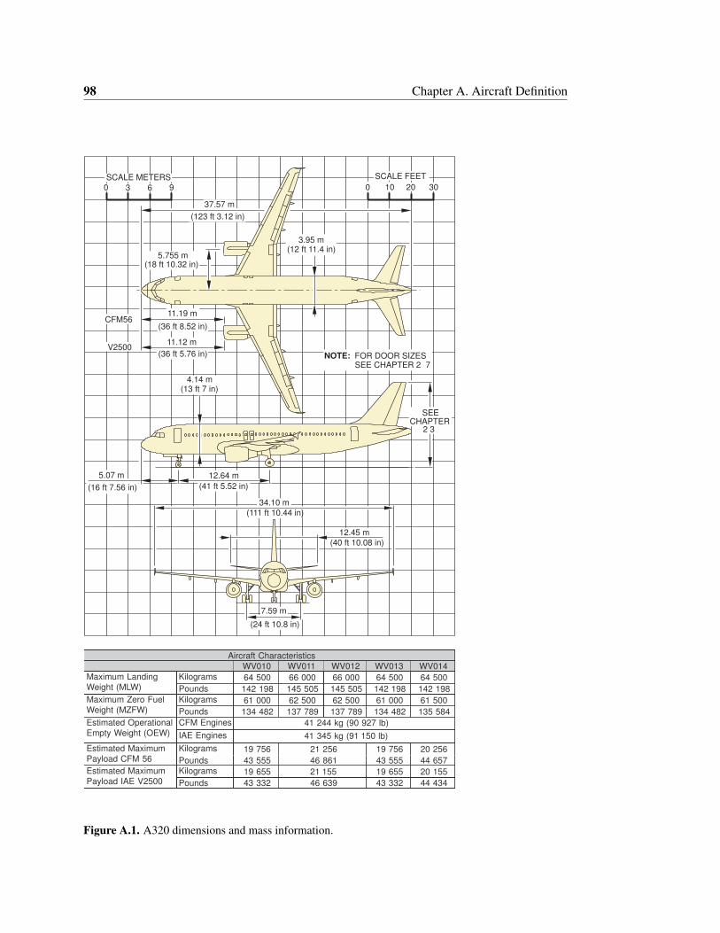
98 Chapter A. Aircraft Definition
(36 ft 5.76 in)
CFM56
V2500
3020100
SCALE FEETSCALE METERS
960 3
12.64 m
37.57 m
(123 ft 3.12 in)
(12 ft 11.4 in)3.95 m
11.19 m
(36 ft 8.52 in)
11.12 m
(13 ft 7 in)4.14 m
(16 ft 7.56 in)
5.07 m
NOTE:
SEE CHAPTER 2� 7FOR DOOR SIZES
SEECHAPTER
(18 ft 10.32 in)5.755 m
(41 ft 5.52 in)
(111 ft 10.44 in)
34.10 m
(40 ft 10.08 in)
12.45 m
(24 ft 10.8 in)
7.59 m
2�3
Aircraft Characteristics
WV010 WV011 WV012 WV013 WV014
Kilograms 64 500 66 000 66 000 64 500 64 500Maximum Landing
Weight (MLW) Pounds 142 198 145 505 145 505 142 198 142 198
Kilograms 61 000 62 500 62 500 61 000 61 500Maximum Zero Fuel
Weight (MZFW) Pounds 134 482 137 789 137 789 134 482 135 584
CFM Engines 41 244 kg (90 927 lb)Estimated Operational
Empty Weight (OEW) IAE Engines 41 345 kg (91 150 lb)
Kilograms 19 756 21 256 19 756 20 256Estimated Maximum
Payload CFM 56 Pounds 43 555 46 861 43 555 44 657
Kilograms 19 655 21 155 19 655 20 155Estimated Maximum
Payload IAE V2500 Pounds 43 332 46 639 43 332 44 434
Figure A.1. A320 dimensions and mass information.
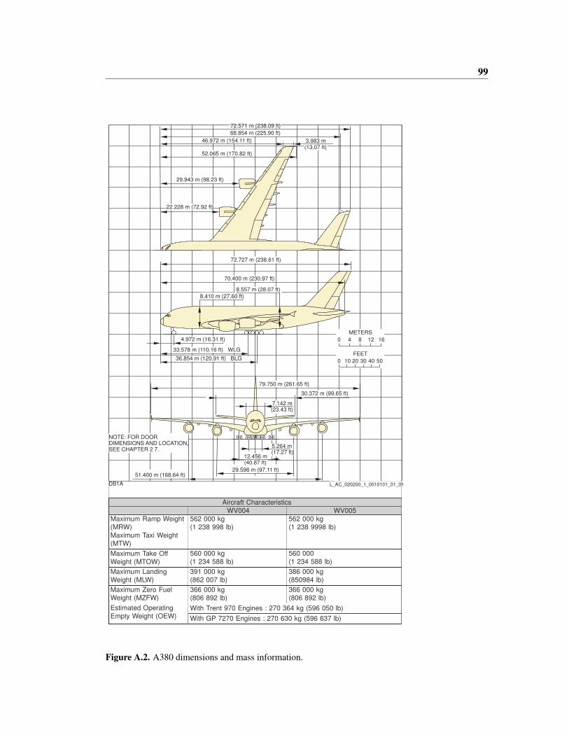
99
DB1A
0 4 8 12 16
METERS
0 10 20 30 40 50
FEET
NOTE: FOR DOORDIMENSIONS AND LOCATION,SEE CHAPTER 2�7.
68.854 m (225.90 ft)
29.598 m (97.11 ft)
7.142 m(23.43 ft)
30.372 m (99.65 ft)
79.750 m (261.65 ft)
12.456 m(40.87 ft)
33.578 m (110.16 ft) � WLG
36.854 m (120.91 ft) � BLG
5.264 m(17.27 ft)
51.400 m (168.64 ft)
4.972 m (16.31 ft)
29.943 m (98.23 ft)
22.228 m (72.92 ft)
72.727 m (238.61 ft)
70.400 m (230.97 ft)
8.410 m (27.60 ft)
8.557 m (28.07 ft)
46.972 m (154.11 ft)
72.571 m (238.09 ft)
3.983 m(13.07 ft)
L_AC_020200_1_0010101_01_01
52.065 m (170.82 ft)
Aircraft Characteristics
WV004 WV005
Maximum Ramp Weight
(MRW)
Maximum Taxi Weight
(MTW)
562 000 kg
(1 238 998 lb)
562 000 kg
(1 238 9998 lb)
Maximum Take Off
Weight (MTOW)
560 000 kg
(1 234 588 lb)
560 000
(1 234 588 lb)
Maximum Landing
Weight (MLW)
391 000 kg
(862 007 lb)
386 000 kg
(850984 lb)
Maximum Zero Fuel
Weight (MZFW)
366 000 kg
(806 892 lb)
366 000 kg
(806 892 lb)
With Trent 970 Engines : 270 364 kg (596 050 lb)Estimated Operating
Empty Weight (OEW) With GP 7270 Engines : 270 630 kg (596 637 lb)
Figure A.2. A380 dimensions and mass information.
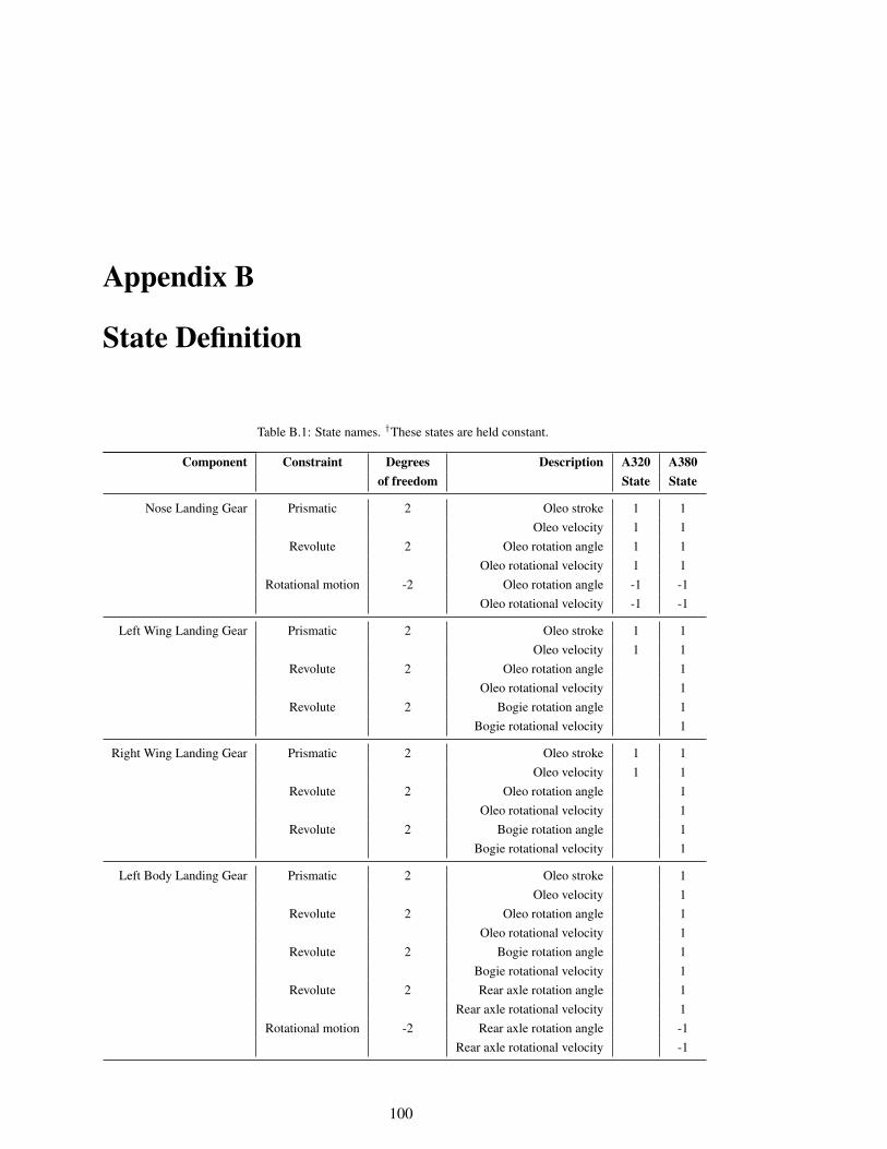
Appendix B
State Definition
Table B.1: State names. †These states are held constant.
Component Constraint Degrees Description A320 A380of freedom State State
Nose Landing Gear Prismatic 2 Oleo stroke 1 1Oleo velocity 1 1
Revolute 2 Oleo rotation angle 1 1Oleo rotational velocity 1 1
Rotational motion -2 Oleo rotation angle -1 -1Oleo rotational velocity -1 -1
Left Wing Landing Gear Prismatic 2 Oleo stroke 1 1Oleo velocity 1 1
Revolute 2 Oleo rotation angle 1Oleo rotational velocity 1
Revolute 2 Bogie rotation angle 1Bogie rotational velocity 1
Right Wing Landing Gear Prismatic 2 Oleo stroke 1 1Oleo velocity 1 1
Revolute 2 Oleo rotation angle 1Oleo rotational velocity 1
Revolute 2 Bogie rotation angle 1Bogie rotational velocity 1
Left Body Landing Gear Prismatic 2 Oleo stroke 1Oleo velocity 1
Revolute 2 Oleo rotation angle 1Oleo rotational velocity 1
Revolute 2 Bogie rotation angle 1Bogie rotational velocity 1
Revolute 2 Rear axle rotation angle 1Rear axle rotational velocity 1
Rotational motion -2 Rear axle rotation angle -1Rear axle rotational velocity -1
100
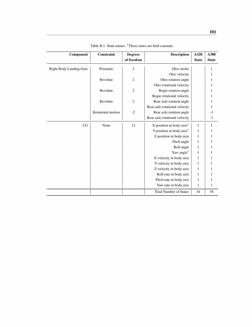
101
Table B.1: State names. †These states are held constant.
Component Constraint Degrees Description A320 A380of freedom State State
Right Body Landing Gear Prismatic 2 Oleo stroke 1Oleo velocity 1
Revolute 2 Oleo rotation angle 1Oleo rotational velocity 1
Revolute 2 Bogie rotation angle 1Bogie rotational velocity 1
Revolute 2 Rear axle rotation angle 1Rear axle rotational velocity 1
Rotational motion -2 Rear axle rotation angle -1Rear axle rotational velocity -1
CG None 12 X-position in body-axis† 1 1Y-position in body-axis† 1 1Z-position in body-axis 1 1
Pitch angle 1 1Roll angle 1 1
Yaw angle† 1 1X-velocity in body-axis 1 1Y-velocity in body-axis 1 1Z-velocity in body-axis 1 1
Roll-rate in body axis 1 1Pitch-rate in body axis 1 1Yaw-rate in body axis 1 1
Total Number of States 18 38
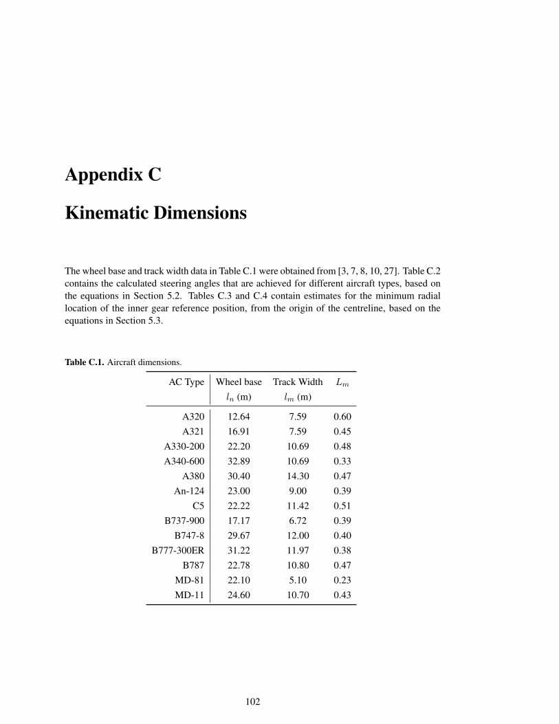
Appendix C
Kinematic Dimensions
The wheel base and track width data in Table C.1 were obtained from [3, 7, 8, 10, 27]. Table C.2contains the calculated steering angles that are achieved for different aircraft types, based onthe equations in Section 5.2. Tables C.3 and C.4 contain estimates for the minimum radiallocation of the inner gear reference position, from the origin of the centreline, based on theequations in Section 5.3.
Table C.1. Aircraft dimensions.
AC Type Wheel base Track Width Lm
ln (m) lm (m)
A320 12.64 7.59 0.60A321 16.91 7.59 0.45
A330-200 22.20 10.69 0.48A340-600 32.89 10.69 0.33
A380 30.40 14.30 0.47An-124 23.00 9.00 0.39
C5 22.22 11.42 0.51B737-900 17.17 6.72 0.39
B747-8 29.67 12.00 0.40B777-300ER 31.22 11.97 0.38
B787 22.78 10.80 0.47MD-81 22.10 5.10 0.23MD-11 24.60 10.70 0.43
102
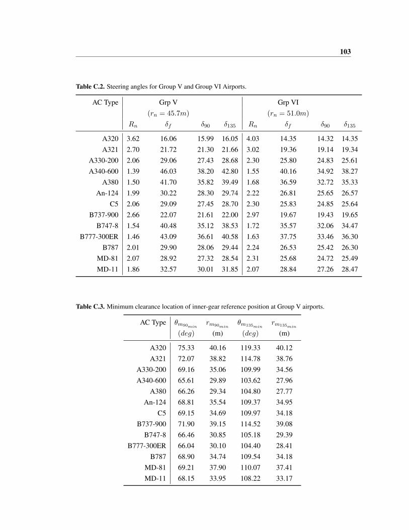
103
Table C.2. Steering angles for Group V and Group VI Airports.
AC Type Grp V Grp VI(rn = 45.7m) (rn = 51.0m)
Rn δf δ90 δ135 Rn δf δ90 δ135
A320 3.62 16.06 15.99 16.05 4.03 14.35 14.32 14.35A321 2.70 21.72 21.30 21.66 3.02 19.36 19.14 19.34
A330-200 2.06 29.06 27.43 28.68 2.30 25.80 24.83 25.61A340-600 1.39 46.03 38.20 42.80 1.55 40.16 34.92 38.27
A380 1.50 41.70 35.82 39.49 1.68 36.59 32.72 35.33An-124 1.99 30.22 28.30 29.74 2.22 26.81 25.65 26.57
C5 2.06 29.09 27.45 28.70 2.30 25.83 24.85 25.64B737-900 2.66 22.07 21.61 22.00 2.97 19.67 19.43 19.65
B747-8 1.54 40.48 35.12 38.53 1.72 35.57 32.06 34.47B777-300ER 1.46 43.09 36.61 40.58 1.63 37.75 33.46 36.30
B787 2.01 29.90 28.06 29.44 2.24 26.53 25.42 26.30MD-81 2.07 28.92 27.32 28.54 2.31 25.68 24.72 25.49MD-11 1.86 32.57 30.01 31.85 2.07 28.84 27.26 28.47
Table C.3. Minimum clearance location of inner-gear reference position at Group V airports.
AC Type θm90minrm90min
θm135minrm135min
(deg) (m) (deg) (m)
A320 75.33 40.16 119.33 40.12A321 72.07 38.82 114.78 38.76
A330-200 69.16 35.06 109.99 34.56A340-600 65.61 29.89 103.62 27.96
A380 66.26 29.34 104.80 27.77An-124 68.81 35.54 109.37 34.95
C5 69.15 34.69 109.97 34.18B737-900 71.90 39.15 114.52 39.08
B747-8 66.46 30.85 105.18 29.39B777-300ER 66.04 30.10 104.40 28.41
B787 68.90 34.74 109.54 34.18MD-81 69.21 37.90 110.07 37.41MD-11 68.15 33.95 108.22 33.17
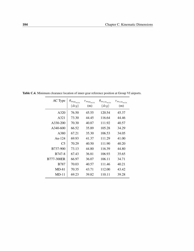
104 Chapter C. Kinematic Dimensions
Table C.4. Minimum clearance location of inner-gear reference position at Group VI airports.
AC Type θm90minrm90min
θm135minrm135min
(deg) (m) (deg) (m)
A320 76.50 45.55 120.54 45.37A321 73.30 44.45 116.64 44.46
A330-200 70.30 40.87 111.92 40.57A340-600 66.52 35.89 105.28 34.29
A380 67.21 35.30 106.53 34.05An-124 69.93 41.37 111.29 41.00
C5 70.29 40.50 111.90 40.20B737-900 73.13 44.80 116.39 44.80
B747-8 67.43 36.81 106.93 35.65B777-300ER 66.97 36.07 106.11 34.71
B787 70.03 40.57 111.46 40.21MD-81 70.35 43.71 112.00 43.42MD-11 69.23 39.82 110.11 39.28
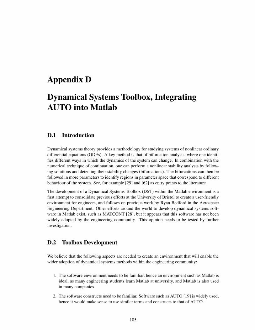
Appendix D
Dynamical Systems Toolbox, IntegratingAUTO into Matlab
D.1 Introduction
Dynamical systems theory provides a methodology for studying systems of nonlinear ordinarydifferential equations (ODEs). A key method is that of bifurcation analysis, where one identi-fies different ways in which the dynamics of the system can change. In combination with thenumerical technique of continuation, one can perform a nonlinear stability analysis by follow-ing solutions and detecting their stability changes (bifurcations). The bifurcations can then befollowed in more parameters to identify regions in parameter space that correspond to differentbehaviour of the system. See, for example [29] and [62] as entry points to the literature.
The development of a Dynamical Systems Toolbox (DST) within the Matlab environment is afirst attempt to consolidate previous efforts at the University of Bristol to create a user-friendlyenvironment for engineers, and follows on previous work by Ryan Bedford in the AerospaceEngineering Department. Other efforts around the world to develop dynamical systems soft-ware in Matlab exist, such as MATCONT [28], but it appears that this software has not beenwidely adopted by the engineering community. This opinion needs to be tested by furtherinvestigation.
D.2 Toolbox Development
We believe that the following aspects are needed to create an environment that will enable thewider adoption of dynamical systems methods within the engineering community:
1. The software environment needs to be familiar, hence an environment such as Matlab isideal, as many engineering students learn Matlab at university, and Matlab is also usedin many companies.
2. The software constructs need to be familiar. Software such as AUTO [19] is widely used,hence it would make sense to use similar terms and constructs to that of AUTO.
105
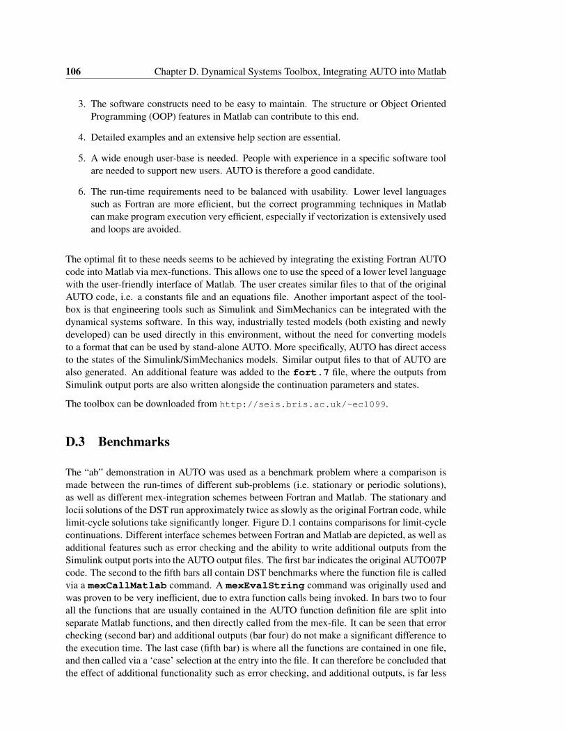
106 Chapter D. Dynamical Systems Toolbox, Integrating AUTO into Matlab
3. The software constructs need to be easy to maintain. The structure or Object OrientedProgramming (OOP) features in Matlab can contribute to this end.
4. Detailed examples and an extensive help section are essential.
5. A wide enough user-base is needed. People with experience in a specific software toolare needed to support new users. AUTO is therefore a good candidate.
6. The run-time requirements need to be balanced with usability. Lower level languagessuch as Fortran are more efficient, but the correct programming techniques in Matlabcan make program execution very efficient, especially if vectorization is extensively usedand loops are avoided.
The optimal fit to these needs seems to be achieved by integrating the existing Fortran AUTOcode into Matlab via mex-functions. This allows one to use the speed of a lower level languagewith the user-friendly interface of Matlab. The user creates similar files to that of the originalAUTO code, i.e. a constants file and an equations file. Another important aspect of the tool-box is that engineering tools such as Simulink and SimMechanics can be integrated with thedynamical systems software. In this way, industrially tested models (both existing and newlydeveloped) can be used directly in this environment, without the need for converting modelsto a format that can be used by stand-alone AUTO. More specifically, AUTO has direct accessto the states of the Simulink/SimMechanics models. Similar output files to that of AUTO arealso generated. An additional feature was added to the fort.7 file, where the outputs fromSimulink output ports are also written alongside the continuation parameters and states.
The toolbox can be downloaded from http://seis.bris.ac.uk/~ec1099.
D.3 Benchmarks
The “ab” demonstration in AUTO was used as a benchmark problem where a comparison ismade between the run-times of different sub-problems (i.e. stationary or periodic solutions),as well as different mex-integration schemes between Fortran and Matlab. The stationary andlocii solutions of the DST run approximately twice as slowly as the original Fortran code, whilelimit-cycle solutions take significantly longer. Figure D.1 contains comparisons for limit-cyclecontinuations. Different interface schemes between Fortran and Matlab are depicted, as well asadditional features such as error checking and the ability to write additional outputs from theSimulink output ports into the AUTO output files. The first bar indicates the original AUTO07Pcode. The second to the fifth bars all contain DST benchmarks where the function file is calledvia a mexCallMatlab command. A mexEvalString command was originally used andwas proven to be very inefficient, due to extra function calls being invoked. In bars two to fourall the functions that are usually contained in the AUTO function definition file are split intoseparate Matlab functions, and then directly called from the mex-file. It can be seen that errorchecking (second bar) and additional outputs (bar four) do not make a significant difference tothe execution time. The last case (fifth bar) is where all the functions are contained in one file,and then called via a ‘case’ selection at the entry into the file. It can therefore be concluded thatthe effect of additional functionality such as error checking, and additional outputs, is far less
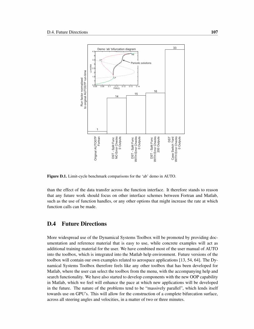
D.4. Future Directions 107
Periodic solutions
Demo ‘ab’ bifurcation diagram
Figure D.1. Limit-cycle benchmark comparisons for the ‘ab’ demo in AUTO.
than the effect of the data transfer across the function interface. It therefore stands to reasonthat any future work should focus on other interface schemes between Fortran and Matlab,such as the use of function handles, or any other options that might increase the rate at whichfunction calls can be made.
D.4 Future Directions
More widespread use of the Dynamical Systems Toolbox will be promoted by providing doc-umentation and reference material that is easy to use, while concrete examples will act asadditional training material for the user. We have combined most of the user manual of AUTOinto the toolbox, which is integrated into the Matlab help environment. Future versions of thetoolbox will contain our own examples related to aerospace applications [13, 54, 64]. The Dy-namical Systems Toolbox therefore feels like any other toolbox that has been developed forMatlab, where the user can select the toolbox from the menu, with the accompanying help andsearch functionality. We have also started to develop components with the new OOP capabilityin Matlab, which we feel will enhance the pace at which new applications will be developedin the future. The nature of the problems tend to be “massively parallel”, which lends itselftowards use on GPU’s. This will allow for the construction of a complete bifurcation surface,across all steering angles and velocities, in a matter of two or three minutes.