Machine Learning with Spark

Giorgio Pedrazzi, CINECA-SCAI

Tools and techniques for massive data

analysis

Roma, 15/12/2016

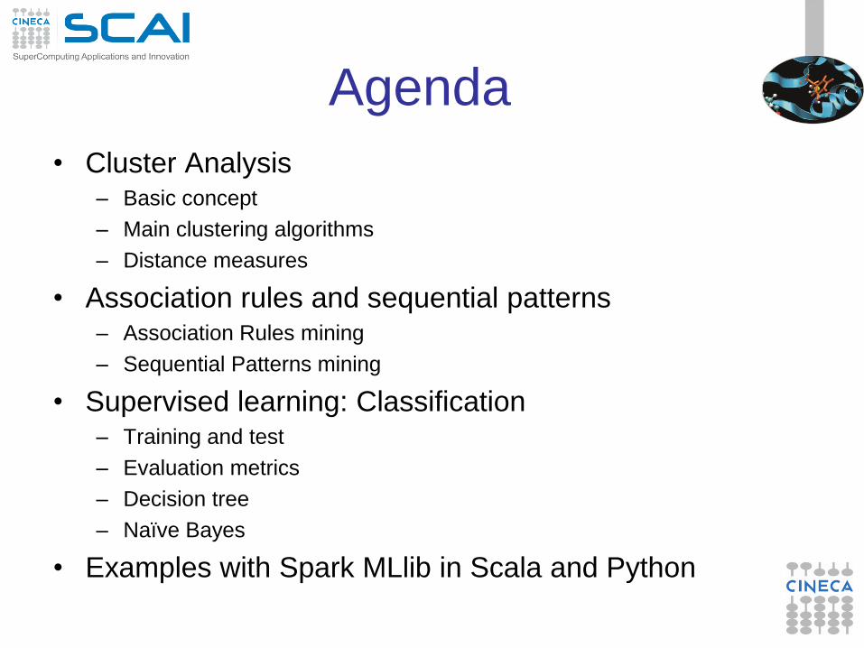
Agenda

• Cluster Analysis – Basic concept

– Main clustering algorithms

– Distance measures

• Association rules and sequential patterns – Association Rules mining

– Sequential Patterns mining

• Supervised learning: Classification – Training and test

– Evaluation metrics

– Decision tree

– Naïve Bayes

• Examples with Spark MLlib in Scala and Python

Cluster analysis • Cluster analysis

– no predefined classes for a training data set

– find similarities between data according to characteristics underlying the data and grouping similar data objects into clusters

– two general tasks: identify the “natural” clustering number and properly grouping objects into “sensible” clusters

• Cluster: A collection/group of data objects/points – similar (or related) to one another within the same group

– dissimilar (or unrelated) to the objects in other groups

• Typical applications – as a stand-alone tool for data exploration

– as a precursor to other supervised learning methods

Typical applications • Scientific applications

– Biology: discover genes with similar functions in DNA microarray data.

– Seismology: grouping earthquake epicenters to identify dangerous

zone.

– …

• Business applications – Marketing: discover distinct groups in customer bases (insurance,

bank, retailers) to develop targeted marketing programs.

– Behavioral analysis: identifying driving styles.

– …

• Internet applications – Social network analysis: in the study of social networks, clustering

may be used to recognize communities within a network.

– Search result ordering: grouping of files or web pages to create

relevant sets of search results.

– …

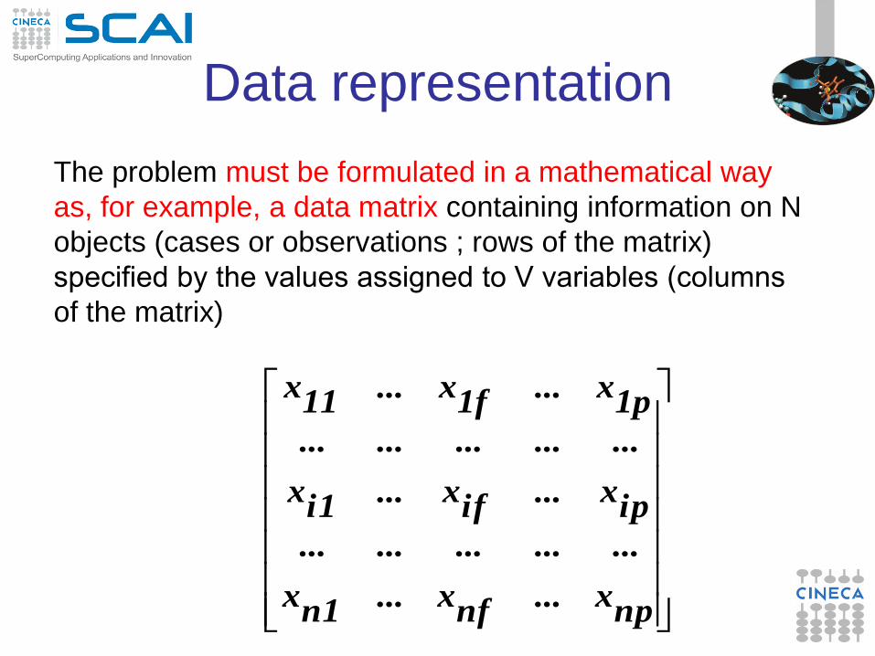
Data representation

The problem must be formulated in a mathematical way

as, for example, a data matrix containing information on N

objects (cases or observations ; rows of the matrix)

specified by the values assigned to V variables (columns

of the matrix)

npx...nfx...n1x

...............

ipx...ifx...i1x

...............

1px...1fx...11x

Cluster Analysis steps • Variable selection

• Preprocessing

• Select a clustering algorithm

• Select a distance or a similarity measure (*)

• Determine the number of clusters (*)

• Validate the analysis

Changing one parameter may result in complete different

cluster results.

(*) if needed by the method used

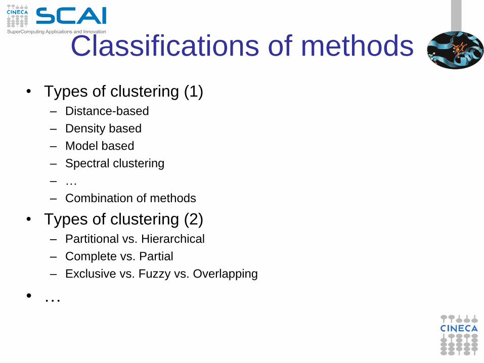
Classifications of methods

• Types of clustering (1) – Distance-based

– Density based

– Model based

– Spectral clustering

– …

– Combination of methods

• Types of clustering (2) – Partitional vs. Hierarchical

– Complete vs. Partial

– Exclusive vs. Fuzzy vs. Overlapping

• …

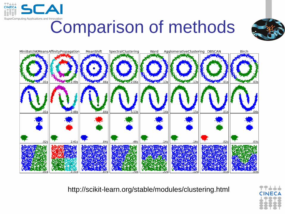
Comparison of methods

http://scikit-learn.org/stable/modules/clustering.html

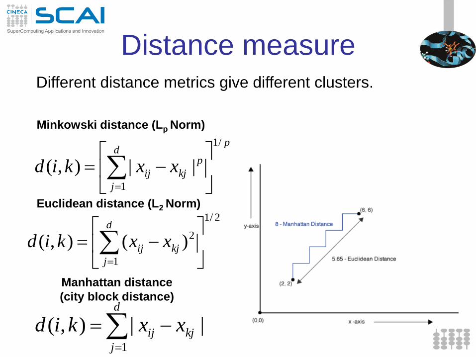
Distance measure

2/1

1

2)(),(

d

j

kjij xxkid

d

j

kjij xxkid1

||),(

Manhattan distance

(city block distance)

Euclidean distance (L2 Norm)

pd

j

p

kjij xxkid

/1

1

||),(

Minkowski distance (Lp Norm)

Different distance metrics give different clusters.

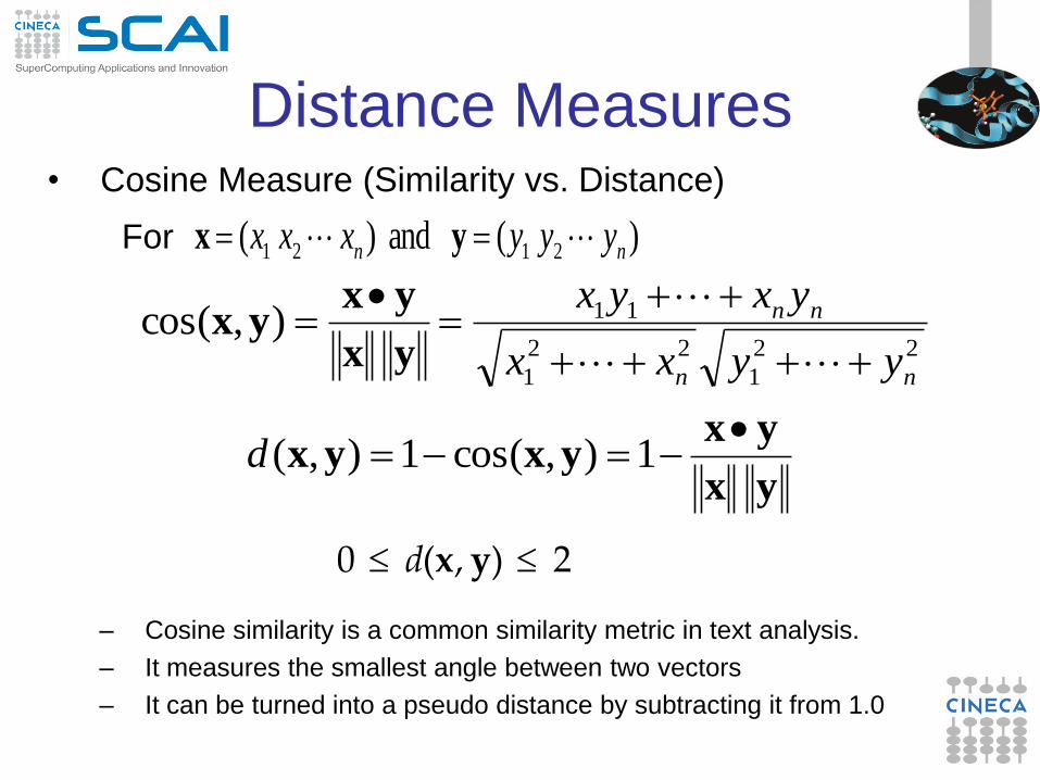
Distance Measures • Cosine Measure (Similarity vs. Distance)

For

– Cosine similarity is a common similarity metric in text analysis.

– It measures the smallest angle between two vectors

– It can be turned into a pseudo distance by subtracting it from 1.0

yx

yxyxyx

yx

yxyx

1),cos(1),(

),cos(22

1

22

1

11

d

yyxx

yxyx

nn

nn

2 ) ,( 0 yxd

) ( and ) ( 2121 nn yyyxxx yx

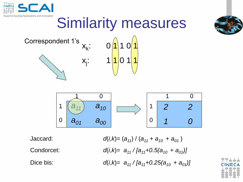
Similarity measures

xk: 0 1 1 0 1

xj: 1 1 0 1 1

Jaccard: d(i,k)= (a11) / (a11 + a10 + a01 )

Condorcet: d(i,k)= a11 / [a11+0.5(a10 + a01)]

Dice bis: d(i,k)= a11 / [a11+0.25(a10 + a01)]

a11 a10

a01 a00

1 0

1

0

2 2

1 0

1 0

1

0

Correspondent 1’s

Distance based (Partitioning)

• Partitioning method: Construct a partition of a database

D of n objects into a set of k clusters

• Given a k, find a partition of k clusters that optimizes the

chosen partitioning criterion

– Global optimal: exhaustively enumerate all partitions

– Heuristic methods: k-means and k-medoids algorithms

– k-means: Each cluster is represented by the center of the cluster

– k-medoids or PAM: Each cluster is represented by one of the objects in

the cluster

Distance based (Hierarchical)

• Agglomerative (bottom-up): – Start with each observation being a single cluster.

– Eventually all observations belong to the same cluster.

• Divisive (top-down):

– Start with all observations belong to the same cluster.

– Eventually each node forms a cluster on its own.

– Could be a recursive application of k-means like algorithms

• Does not require the number of clusters k in advance

• Needs a termination/readout condition

Hierarchical Agglomerative

Clustering • Assumes a similarity function for determining the

similarity of two instances.

• Starts with all instances in a separate cluster and then

repeatedly joins the two clusters that are most similar

until there is only one cluster.

• The history of merging forms a binary tree or hierarchy.

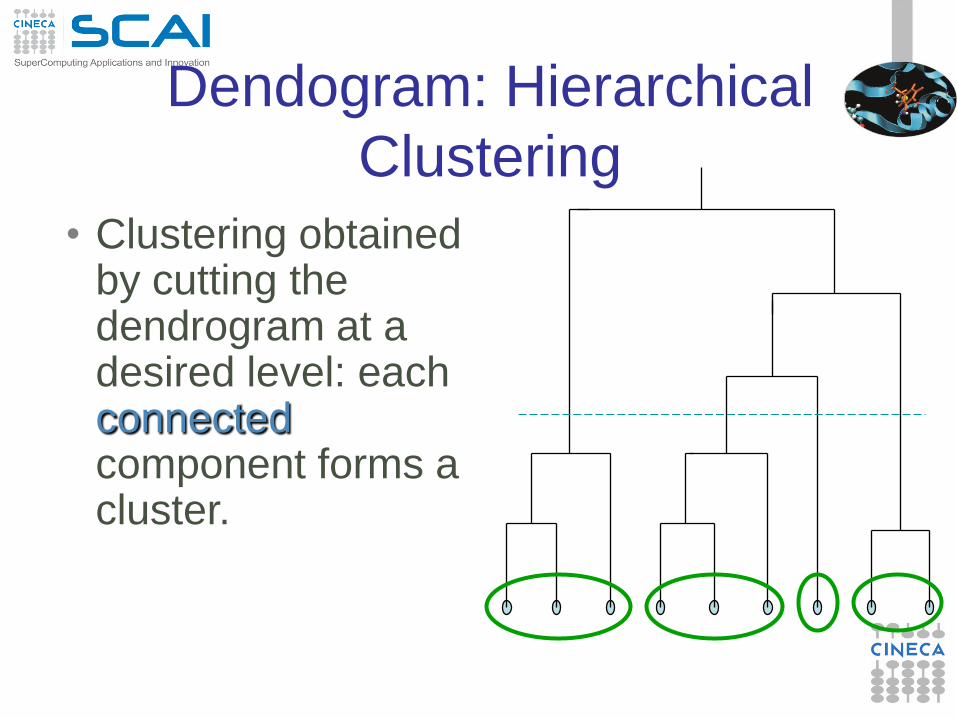
• Clustering obtained by cutting the dendrogram at a desired level: each connected component forms a cluster.

Dendogram: Hierarchical

Clustering

Hierarchical Agglomerative

Clustering (HAC) • Starts with each observation in a separate cluster

– then repeatedly joins the closest pair of clusters, until there is only one

cluster.

• The history of merging forms a binary tree or hierarchy.

How to measure distance of clusters??

Closest pair of clusters

Many variants to defining closest pair of clusters

• Single-link – Distance of the “closest” points (single-link)

• Complete-link – Distance of the “furthest” points

• Centroid – Distance of the centroids (centers of gravity)

• Average-link – Average distance between pairs of elements

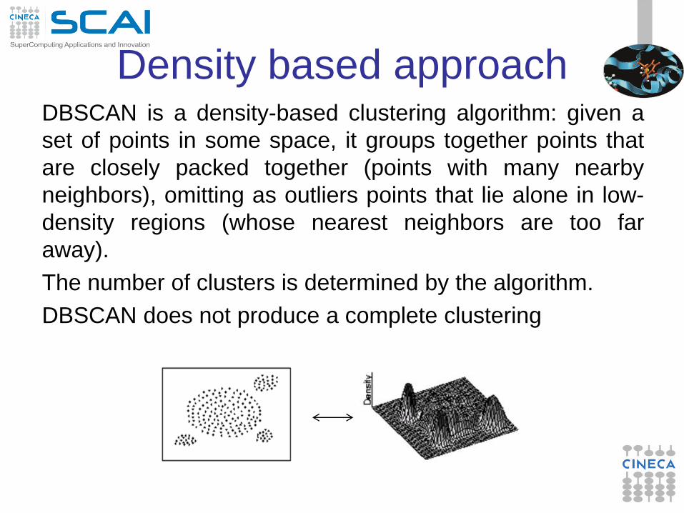
Density based approach DBSCAN is a density-based clustering algorithm: given a

set of points in some space, it groups together points that

are closely packed together (points with many nearby

neighbors), omitting as outliers points that lie alone in low-

density regions (whose nearest neighbors are too far

away).

The number of clusters is determined by the algorithm.

DBSCAN does not produce a complete clustering

Model-based Approach

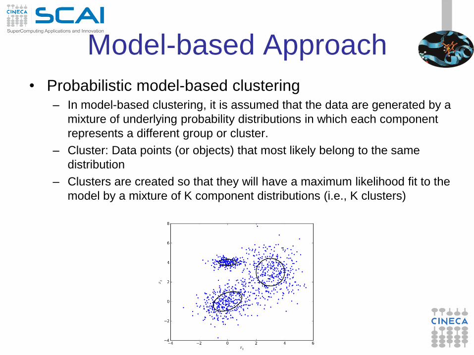
• Probabilistic model-based clustering – In model-based clustering, it is assumed that the data are generated by a

mixture of underlying probability distributions in which each component

represents a different group or cluster.

– Cluster: Data points (or objects) that most likely belong to the same

distribution

– Clusters are created so that they will have a maximum likelihood fit to the

model by a mixture of K component distributions (i.e., K clusters)

Spectral Clustering Approach

• In multivariate statistics, spectral clustering techniques

make use of eigenvalue decomposition (spectrum) of the

similarity matrix of the data to perform dimensionality

reduction before clustering in fewer dimensions. The

similarity matrix is provided as an input and consists of a

quantitative assessment of the relative similarity of each

pair of points in the dataset.

• In application to image segmentation, spectral clustering

is known as segmentation-based object categorization.

21

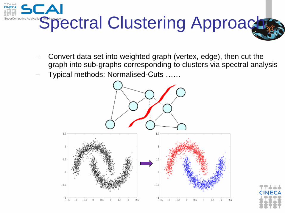
Spectral Clustering Approach

– Convert data set into weighted graph (vertex, edge), then cut the graph into sub-graphs corresponding to clusters via spectral analysis

– Typical methods: Normalised-Cuts ……

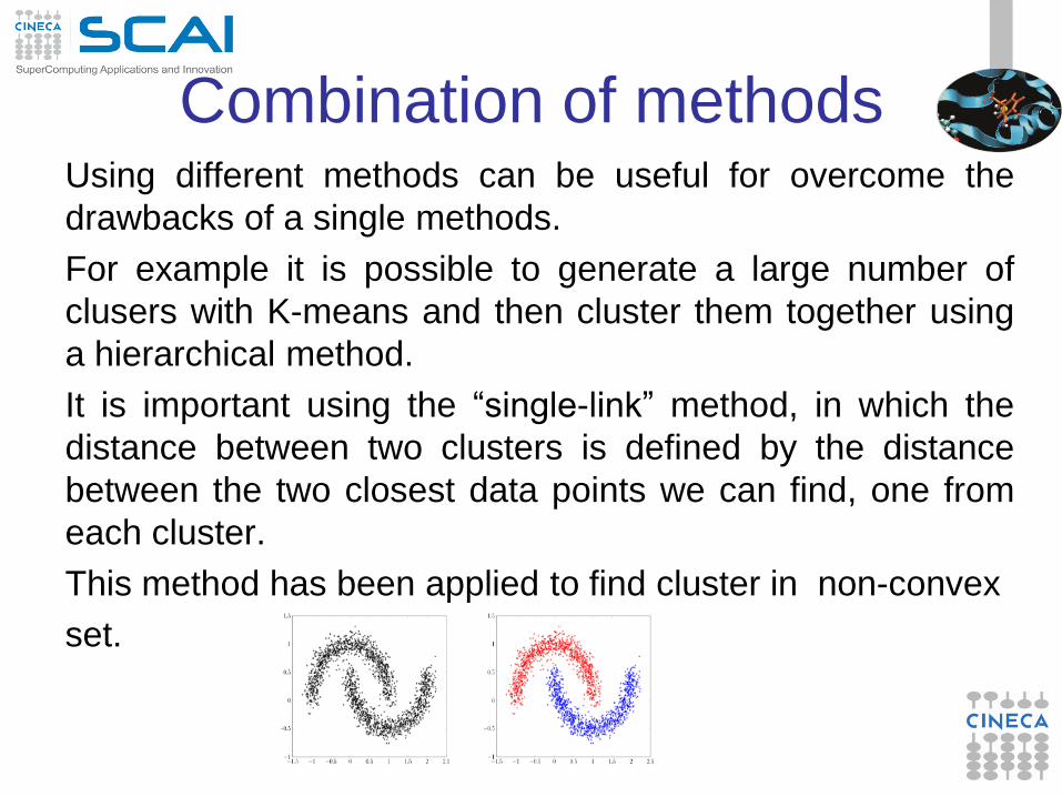
Combination of methods Using different methods can be useful for overcome the

drawbacks of a single methods.

For example it is possible to generate a large number of

clusers with K-means and then cluster them together using

a hierarchical method.

It is important using the “single-link” method, in which the

distance between two clusters is defined by the distance

between the two closest data points we can find, one from

each cluster.

This method has been applied to find cluster in non-convex

set.

Cluster validation

• In supervised classification, the evaluation of the resulting

model is an integral part of model developing process

• For cluster analysis, the analogous question is how to

evaluate the “goodness” of the resulting clusters with the

aim of:

– To avoid finding patterns in noise

– To compare clustering algorithms

– To compare two sets of clusters

– To compare two clusters

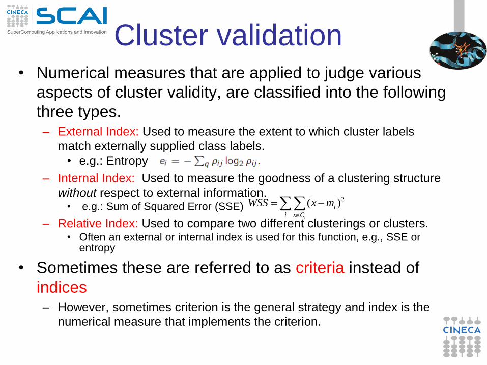
• Numerical measures that are applied to judge various

aspects of cluster validity, are classified into the following

three types. – External Index: Used to measure the extent to which cluster labels

match externally supplied class labels.

• e.g.: Entropy

– Internal Index: Used to measure the goodness of a clustering structure

without respect to external information. • e.g.: Sum of Squared Error (SSE)

– Relative Index: Used to compare two different clusterings or clusters. • Often an external or internal index is used for this function, e.g., SSE or

entropy

• Sometimes these are referred to as criteria instead of

indices – However, sometimes criterion is the general strategy and index is the

numerical measure that implements the criterion.

Cluster validation

i Cx

i

i

mxWSS 2)(

• MLlib is a Spark subproject providing machine learning

primitives:

• MLlib’s goal is to make practical machine learning (ML)

scalable and easy. Besides new algorithms and

performance improvements that we have seen in each

release, a great deal of time and effort has been spent on

making MLlib easy.

• MLlib algorithms – classification: logistic regression, naive Bayes, decision tree, ensemble

of trees (random forests)

– regression: generalized linear regression (GLM)

– collaborative filtering: alternating least squares (ALS)

– clustering: k-means, gaussian mixture, power iteration clustering, latent

Dirichelet allocation

– decomposition: singular value decomposition (SVD), principal

component analysis, singular value decompostion

• Spark packages availables for machine learning at

http://spark-packages.org

Association Rules mining

• Association rule mining is used to find objects or attributes that frequently occur together.

• For example, products that are often bought together during a shopping session (market basket analysis), or queries that tend to occur together during a session on a website’s search engine.

• The unit of “togetherness” when mining association rules is called a transaction. Depending on the problem, a transaction could be a single shopping basket, a single user session on a website, or even a single customer.

• The objects that comprise a transaction are referred to as items in an itemset.

Market Basket Analysis • Basket data consist of collection of transaction date and

items bought in a transaction

• Retail organizations interested in generating qualified decisions and strategy based on analysis of transaction data

– what to put on sale, how to place merchandise on shelves for maximizing profit, customer segmentation based on buying pattern

• Examples. – Rule form: LHS RHS [confidence, support].

– diapers beers [60%, 0.5%]

– “90% of transactions that purchase bread and butter also purchase milk”

– bread and butter milk [90%, 1%]

• https://www.youtube.com/watch?v=N5WurXNec7E&feature=player_embedded

Association rule discovery

problem • Two sub-problems in discovering all association

rules:

– Find all sets of items (itemsets) that have transaction support above

minimum support Itemsets with minimum support are called large

itemsets, and all others small itemsets.

– Generate from each large itemset, rules that use items from the large

itemset.

Given a large itemset Y, and X is a subset of Y

Take the support of Y and divide it by the support of X

If the ratio is at least minconf, then X (Y - X) is satisfied with

confidence factor c

Discovering Large Itemsets • Algorithm for discovering large itemsets make

multiple passes over the data

– In the first pass: count the support of individual items and

determine which of them are large.

– In each subsequent pass:

• start with a set of itemsets found to be large in the previous pass.

• This set is used for generating new potentially large itemsets, called

candidate itemsets

• counts the actual support for these candidate itemsets during the pass

over the data.

– This process continues until no new large itemsets are found.

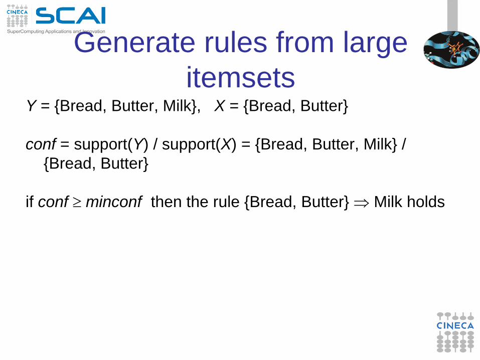
Generate rules from large

itemsets Y = {Bread, Butter, Milk}, X = {Bread, Butter}

conf = support(Y) / support(X) = {Bread, Butter, Milk} /

{Bread, Butter}

if conf minconf then the rule {Bread, Butter} Milk holds

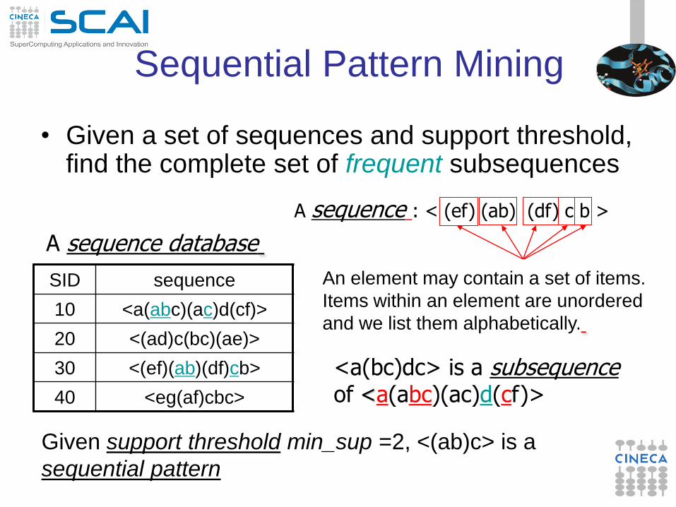
Sequential Pattern Mining

• Given a set of sequences and support threshold, find the complete set of frequent subsequences

A sequence database

A sequence : < (ef) (ab) (df) c b >

An element may contain a set of items.

Items within an element are unordered

and we list them alphabetically.

<a(bc)dc> is a subsequence of <a(abc)(ac)d(cf)>

Given support threshold min_sup =2, <(ab)c> is a

sequential pattern

SID sequence

10 <a(abc)(ac)d(cf)>

20 <(ad)c(bc)(ae)>

30 <(ef)(ab)(df)cb>

40 <eg(af)cbc>

Applications of sequential

pattern mining

• Customer shopping sequences:

– First buy computer, then CD-ROM, and then digital camera, within 3

months.

• Medical treatments, natural disasters (e.g.,

earthquakes), science & eng. processes, stocks and

markets, etc.

• Telephone calling patterns, Weblog click streams

• DNA sequences and gene structures

34

Supervised learning:

classification • Human learning from past experiences.

• A computer does not have “experiences”.

• A computer system learns from data, which represent

some “past experiences” of an application domain.

• Learn a target function that can be used to predict the

values of a discrete class attribute,

• The task is commonly called: Supervised learning,

classification, or inductive learning.

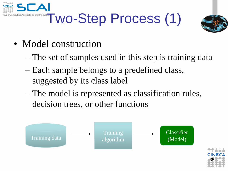
Two-Step Process (1)

• Model construction

– The set of samples used in this step is training data

– Each sample belongs to a predefined class,

suggested by its class label

– The model is represented as classification rules,

decision trees, or other functions

35

Training data Training

algorithm

Classifier

(Model)

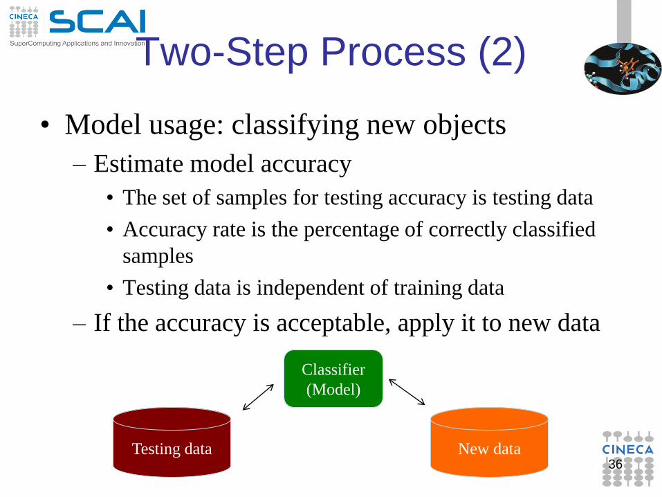
Two-Step Process (2)

• Model usage: classifying new objects

– Estimate model accuracy

• The set of samples for testing accuracy is testing data

• Accuracy rate is the percentage of correctly classified

samples

• Testing data is independent of training data

– If the accuracy is acceptable, apply it to new data

36

Classifier

(Model)

Testing data New data

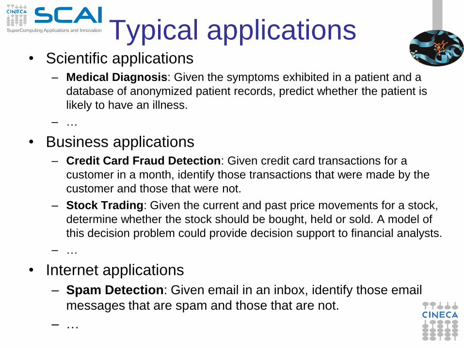
Typical applications • Scientific applications

– Medical Diagnosis: Given the symptoms exhibited in a patient and a

database of anonymized patient records, predict whether the patient is

likely to have an illness.

– …

• Business applications – Credit Card Fraud Detection: Given credit card transactions for a

customer in a month, identify those transactions that were made by the

customer and those that were not.

– Stock Trading: Given the current and past price movements for a stock,

determine whether the stock should be bought, held or sold. A model of

this decision problem could provide decision support to financial analysts.

– …

• Internet applications

– Spam Detection: Given email in an inbox, identify those email

messages that are spam and those that are not.

– …

Classification Techniques

• Decision Tree based Methods

• Ensemble methods

• Naïve Bayes and Bayesian Belief Networks

• Rule-based Methods

• Memory based reasoning

• Neural Networks

• Support Vector Machines

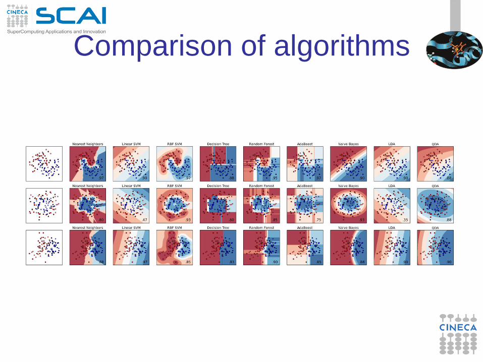
Comparison of algorithms

Training and test a classifier

Is the model able to generalize? Can it deal with unseen

data, or does it overfit the data? Test on hold-out data:

• split data to be modeled in training and test set

• train the model on training set

• evaluate the model on the training set

• evaluate the model on the test set

• difference between the fit on training data and test

data measures the model’s ability to generalize

Methods to create training and

test data

• Fixed – Leave out random N% of the data

• K-fold Cross-Validation

– Select K folds without replace

• Leave-One-Out Cross Validation

– Special case of CV

• Bootstrap – Generate new training sets by sampling with replacement

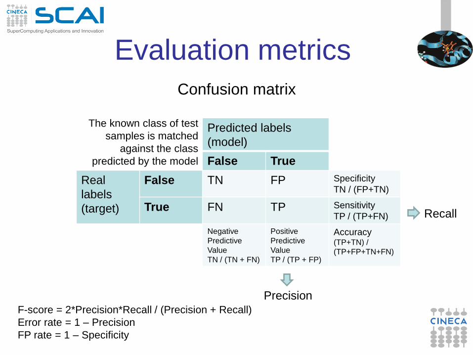
Evaluation metrics

Confusion matrix

Predicted labels

(model)

False True

Real

labels

(target)

False TN FP Specificity

TN / (FP+TN)

True FN TP Sensitivity

TP / (TP+FN)

Negative

Predictive

Value

TN / (TN + FN)

Positive

Predictive

Value

TP / (TP + FP)

Accuracy (TP+TN) /

(TP+FP+TN+FN)

Recall

Precision F-score = 2*Precision*Recall / (Precision + Recall)

Error rate = 1 – Precision

FP rate = 1 – Specificity

The known class of test

samples is matched

against the class

predicted by the model

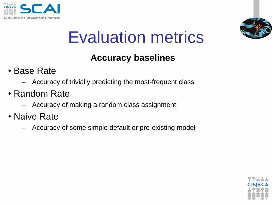
Evaluation metrics

Accuracy baselines

• Base Rate – Accuracy of trivially predicting the most-frequent class

• Random Rate – Accuracy of making a random class assignment

• Naive Rate – Accuracy of some simple default or pre-existing model

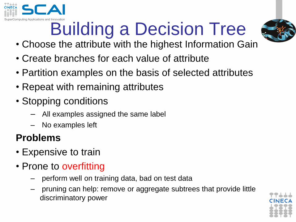
Building a Decision Tree • Choose the attribute with the highest Information Gain

• Create branches for each value of attribute

• Partition examples on the basis of selected attributes

• Repeat with remaining attributes

• Stopping conditions

– All examples assigned the same label

– No examples left

Problems

• Expensive to train

• Prone to overfitting – perform well on training data, bad on test data

– pruning can help: remove or aggregate subtrees that provide little

discriminatory power

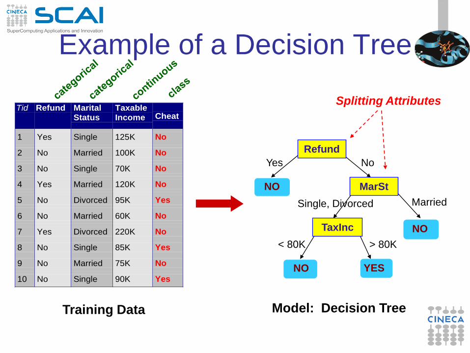
Example of a Decision Tree

Tid Refund MaritalStatus

TaxableIncome Cheat

1 Yes Single 125K No

2 No Married 100K No

3 No Single 70K No

4 Yes Married 120K No

5 No Divorced 95K Yes

6 No Married 60K No

7 Yes Divorced 220K No

8 No Single 85K Yes

9 No Married 75K No

10 No Single 90K Yes10

Refund

MarSt

TaxInc

YES NO

NO

NO

Yes No

Married Single, Divorced

< 80K > 80K

Splitting Attributes

Training Data Model: Decision Tree

Bootstrap

Given a dataset of size N

Draw N samples with replacement to create a new

dataset

Repeat ~1000 times

You now have ~1000 sample datasets

All drawn from the same population

You can compute ~1000 sample statistics

You can interpret these as repeated experiments

Very elegant use of computational resources

The bootstrap allows you to simulate repeated statistical

experiments

Statistics computed from bootstrap samples are typically

unbiased estimators

Ensembles

Combining classifiers The output of a set of classifiers can be combined to

derive a stronger classifier

(e.g. average results from different models)

Better classification performance than individual

classifiers

More resilience to noise

Time consuming

Models become difficult to explain

Bagging

Draw N bootstrap samples

Retrain the model on each sample

Average the results

Regression: Averaging

Classification: Majority vote

Works great for overfit models

Boosting: instead of selecting data points randomly,

favor the misclassified points

Initialize the weights

Repeat:

Resample with respect to weights

Retrain the model

Recompute weights

The disadvantage of boosting, relative to big data, is that it’s inherently

sequential (weights in time t depend from weights in time t-1; while in bagging

everything can go parallel)

Random forest

Ensemble method based on decision trees Repeat k times:

Draw a bootstrap sample from the dataset

Train a decision tree

Until the tree is maximum size

Choose next leaf node

Select m attributes at random from the p available

Pick the best attribute/split as usual

Measure out-of-bag error

Evaluate against the samples that were not selected in the

bootstrap

Provides measures of strength (inverse error rate), correlation

between trees, and variable importance

Make a prediction by majority vote among the k trees

Random Forests

General and powerful technique

Easy to parallelize

Trees are built independently

Work on categorical attributes

Handles “small n big p” problems naturally

A subset of attributes are selected by importance

Avoids overfitting (ensemble of models)

Decision Trees and Random Forests

Representation

Decision Trees

Sets of decision trees with majority vote

Evaluation

Accuracy

Random forests: out-of-bag error

Optimization

Information Gain or Gini Index to measure impurity and

select best attributes

Naïve Bayesian Classfication

Bayes theorem:

P(C|X) = P(X|C)·P(C) / P(X)

P(X) is constant for all classes

P(C) = relative freq of class C samples

C such that P(C|X) is maximum =

C such that P(X|C)·P(C) is maximum

Problem: computing P(X|C) is unfeasible!

Naïve Bayesian Classification

• Here's where the "Naive" comes in. We're going to assume that the

different features of the data are independent of each other, conditional

on C=c.

• P(x1,…,xk|C) = P(x1|C)·…·P(xk|C)

• By making the decision to completely ignore the correlations between

features, this method is blissfully unaware of the primary difficulty of high-

dimensional (high-p) datasets, and training Naive Bayes classifiers

becomes extremely easy.

If i-th attribute is categorical:

P(xi|C) is estimated as the relative freq of samples having value xi

as i-th attribute in class C

If i-th attribute is continuous:

P(xi|C) is estimated thruogh a Gaussian density function