Lecture’7:’’...
45
Lecture 7 - Fei-Fei Li Lecture 7: Finding Features (part 2/2) Professor FeiFei Li Stanford Vision Lab 2Oct14 1
Transcript of Lecture’7:’’...
Lecture 7 - !!!
Fei-Fei Li!
Lecture 7: Finding Features (part 2/2)
Professor Fei-‐Fei Li Stanford Vision Lab
2-‐Oct-‐14 1
Lecture 7 - !!!
Fei-Fei Li!
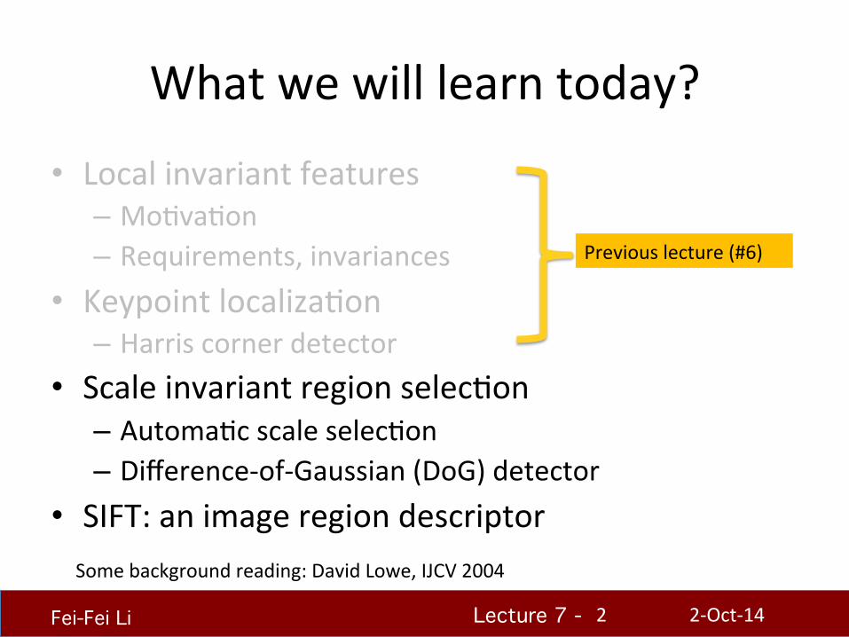
What we will learn today?
• Local invariant features – MoHvaHon – Requirements, invariances
• Keypoint localizaHon – Harris corner detector
• Scale invariant region selecHon – AutomaHc scale selecHon – Difference-‐of-‐Gaussian (DoG) detector
• SIFT: an image region descriptor
2-‐Oct-‐14 2
Previous lecture (#6)
Some background reading: David Lowe, IJCV 2004
Lecture 7 - !!!
Fei-Fei Li!
A quick review
• Local invariant features – MoHvaHon – Requirements, invariances
• Keypoint localizaHon – Harris corner detector
• Scale invariant region selecHon – AutomaHc scale selecHon – Difference-‐of-‐Gaussian (DoG) detector
• SIFT: an image region descriptor
2-‐Oct-‐14 3
Lecture 7 - !!!
Fei-Fei Li!
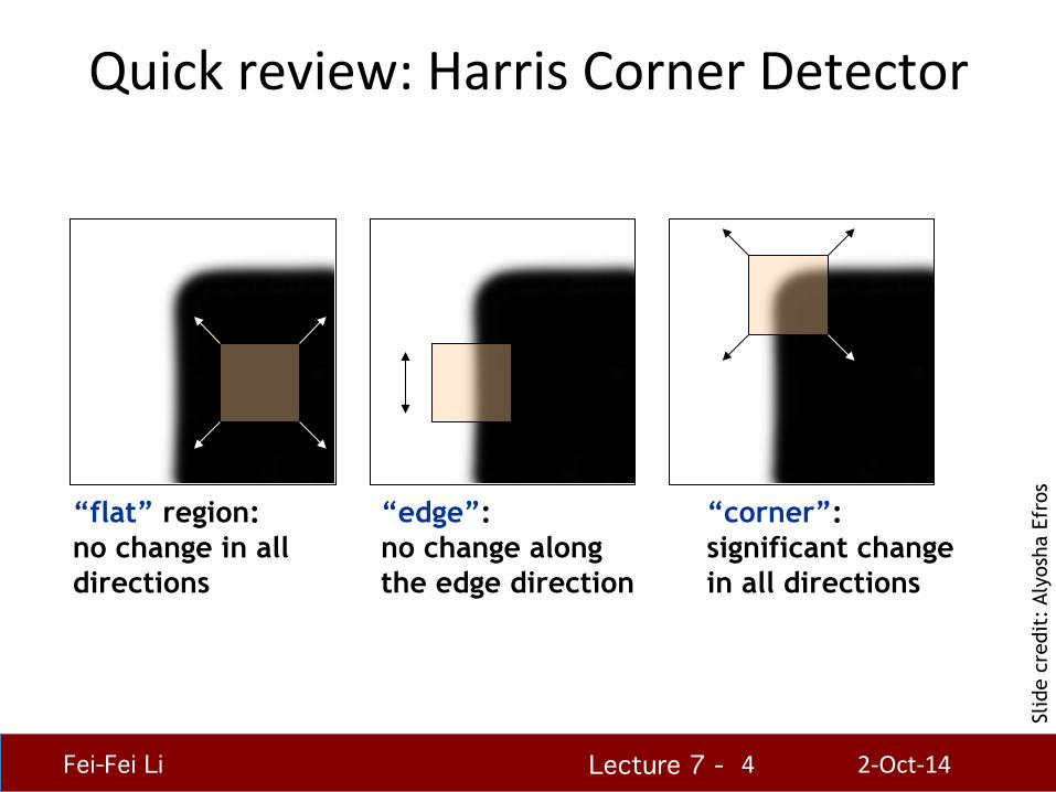
Quick review: Harris Corner Detector
2-‐Oct-‐14 4
“edge”: no change along the edge direction
“corner”: significant change in all directions
“flat” region: no change in all directions
Slid
e cr
edit
: Al
yosh
a Ef
ros
Lecture 7 - !!!
Fei-Fei Li!
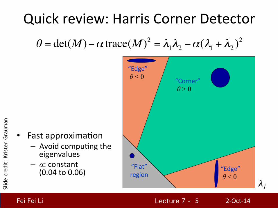
Quick review: Harris Corner Detector
2-‐Oct-‐14 5
• Fast approximaHon – Avoid compuHng the eigenvalues
– α: constant (0.04 to 0.06)
θ = det(M )−α trace(M )2 = λ1λ2 −α(λ1 +λ2 )2
Slid
e cr
edit
: Kr
iste
n G
raum
an
“Corner” θ > 0
“Edge” θ < 0
“Edge” θ < 0
“Flat” region
λ1
Lecture 7 - !!!
Fei-Fei Li!
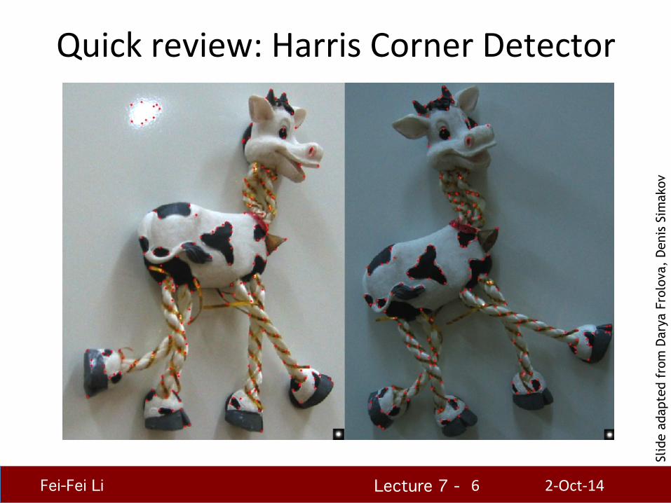
Quick review: Harris Corner Detector
2-‐Oct-‐14 6
Slid
e ad
apte
d fr
om D
arya
Fro
lova
, D
enis
Sim
akov
Lecture 7 - !!!
Fei-Fei Li!
Quick review: Harris Corner Detector
2-‐Oct-‐14 7
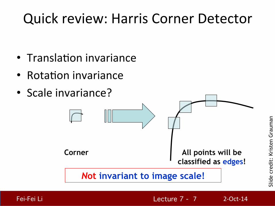
• TranslaHon invariance • RotaHon invariance • Scale invariance?
Not invariant to image scale!
All points will be classified as edges!
Corner
Slid
e cr
edit
: Kr
iste
n G
raum
an
Lecture 7 - !!!
Fei-Fei Li!
What we will learn today?
• Local invariant features – MoHvaHon – Requirements, invariances
• Keypoint localizaHon – Harris corner detector
• Scale invariant region selecHon – AutomaHc scale selecHon – Difference-‐of-‐Gaussian (DoG) detector
• SIFT: an image region descriptor
2-‐Oct-‐14 8
Lecture 7 - !!!
Fei-Fei Li!
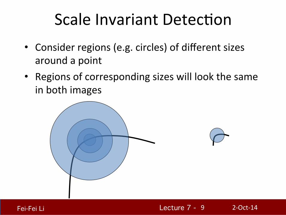
Scale Invariant DetecHon • Consider regions (e.g. circles) of different sizes around a point
• Regions of corresponding sizes will look the same in both images
2-‐Oct-‐14 9
Lecture 7 - !!!
Fei-Fei Li!
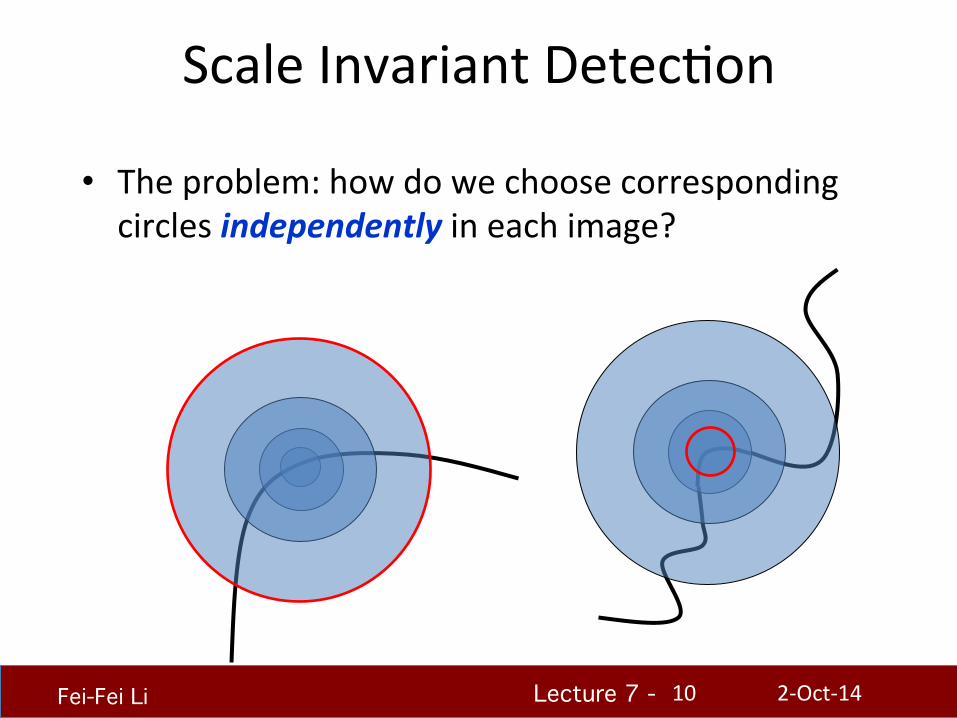
Scale Invariant DetecHon
• The problem: how do we choose corresponding circles independently in each image?
2-‐Oct-‐14 10
Lecture 7 - !!!
Fei-Fei Li!
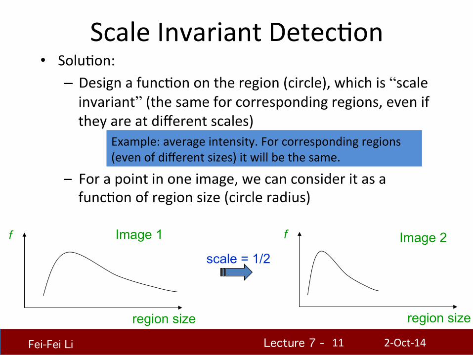
Scale Invariant DetecHon • SoluHon:
– Design a funcHon on the region (circle), which is “scale invariant” (the same for corresponding regions, even if they are at different scales)
Example: average intensity. For corresponding regions (even of different sizes) it will be the same.
scale = 1/2
– For a point in one image, we can consider it as a funcHon of region size (circle radius)
f
region size
Image 1 f
region size
Image 2
2-‐Oct-‐14 11
Lecture 7 - !!!
Fei-Fei Li!
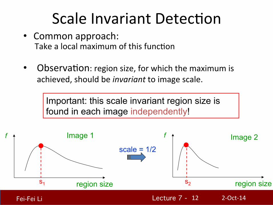
Scale Invariant DetecHon • Common approach:
scale = 1/2
f
region size
Image 1 f
region size
Image 2
Take a local maximum of this funcHon
• ObservaHon: region size, for which the maximum is achieved, should be invariant to image scale.
s1 s2
Important: this scale invariant region size is found in each image independently!
2-‐Oct-‐14 12
Lecture 7 - !!!
Fei-Fei Li!
Scale Invariant DetecHon
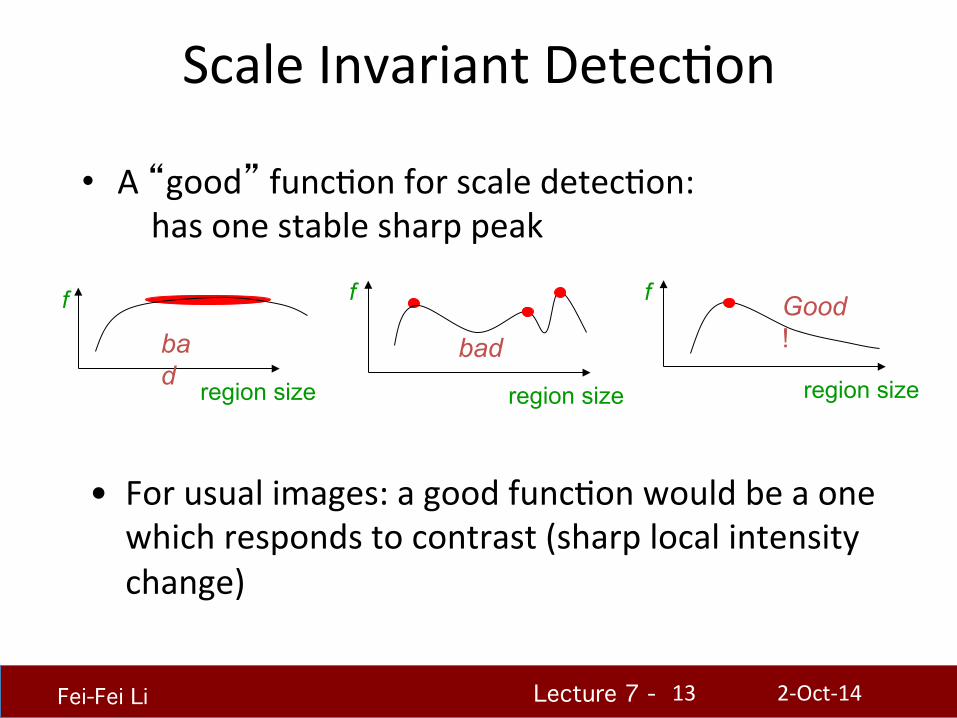
• A “good” funcHon for scale detecHon: has one stable sharp peak
f
region size
bad
f
region size
bad
f
region size
Good !
• For usual images: a good funcHon would be a one which responds to contrast (sharp local intensity change)
2-‐Oct-‐14 13
Lecture 7 - !!!
Fei-Fei Li!
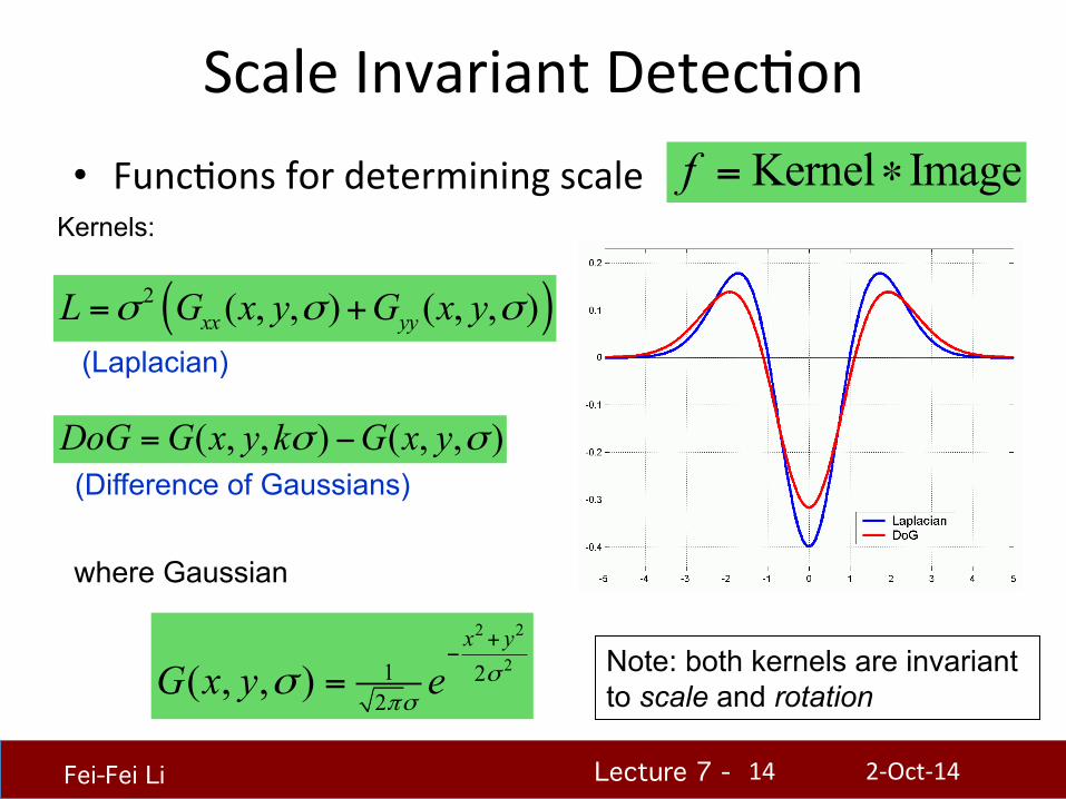
Scale Invariant DetecHon • FuncHons for determining scale
2 2
21 22
( , , )x y
G x y e σπσ
σ+
−
=
( )2 ( , , ) ( , , )xx yyL G x y G x yσ σ σ= +
( , , ) ( , , )DoG G x y k G x yσ σ= −
Kernel Imagef = ∗Kernels:
where Gaussian
Note: both kernels are invariant to scale and rotation
(Laplacian)
(Difference of Gaussians)
2-‐Oct-‐14 14
Lecture 7 - !!!
Fei-Fei Li!
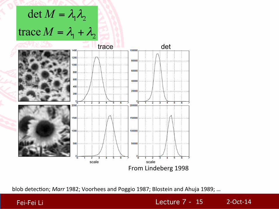
1 2
1 2
dettrace
MM
λ λ
λ λ
=
= +
blob detecHon; Marr 1982; Voorhees and Poggio 1987; Blostein and Ahuja 1989; …
trace det
scale scale
From Lindeberg 1998
2-‐Oct-‐14 15
Lecture 7 - !!!
Fei-Fei Li!
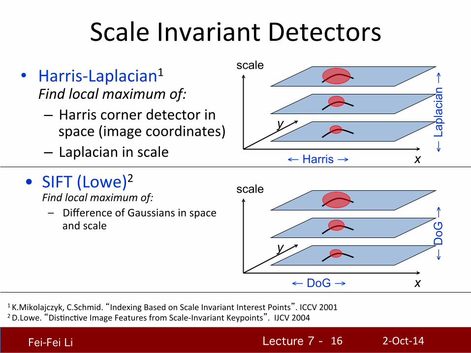
Scale Invariant Detectors • Harris-‐Laplacian1
Find local maximum of: – Harris corner detector in space (image coordinates)
– Laplacian in scale
1 K.Mikolajczyk, C.Schmid. “Indexing Based on Scale Invariant Interest Points”. ICCV 2001 2 D.Lowe. “DisHncHve Image Features from Scale-‐Invariant Keypoints”. IJCV 2004
scale
x
y
← Harris →
← L
apla
cian
→
• SIFT (Lowe)2 Find local maximum of: – Difference of Gaussians in space
and scale
scale
x
y
← DoG →
← D
oG →
2-‐Oct-‐14 16
Lecture 7 - !!!
Fei-Fei Li!
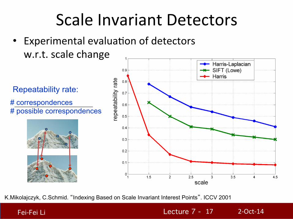
Scale Invariant Detectors
K.Mikolajczyk, C.Schmid. “Indexing Based on Scale Invariant Interest Points”. ICCV 2001
• Experimental evaluaHon of detectors w.r.t. scale change
Repeatability rate: # correspondences # possible correspondences
2-‐Oct-‐14 17
Lecture 7 - !!!
Fei-Fei Li!
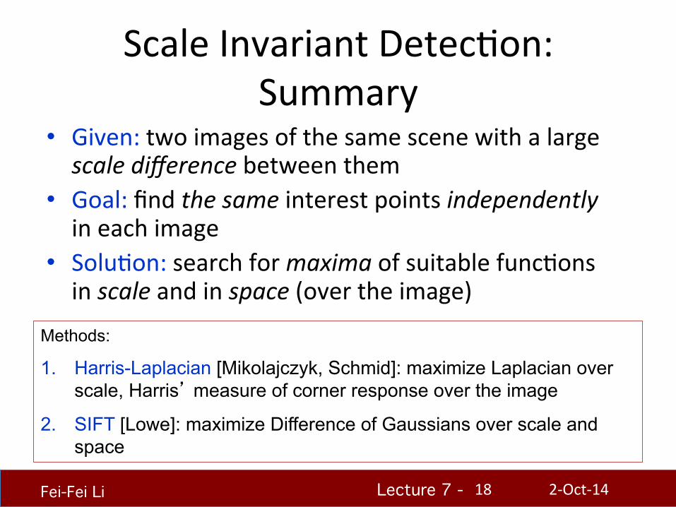
Scale Invariant DetecHon: Summary
• Given: two images of the same scene with a large scale difference between them
• Goal: find the same interest points independently in each image
• SoluHon: search for maxima of suitable funcHons in scale and in space (over the image)
Methods:
1. Harris-Laplacian [Mikolajczyk, Schmid]: maximize Laplacian over scale, Harris’ measure of corner response over the image
2. SIFT [Lowe]: maximize Difference of Gaussians over scale and space
2-‐Oct-‐14 18
Lecture 7 - !!!
Fei-Fei Li!
What we will learn today?
• Local invariant features – MoHvaHon – Requirements, invariances
• Keypoint localizaHon – Harris corner detector
• Scale invariant region selecHon – AutomaHc scale selecHon – Difference-‐of-‐Gaussian (DoG) detector
• SIFT: an image region descriptor
2-‐Oct-‐14 19
Lecture 7 - !!!
Fei-Fei Li!
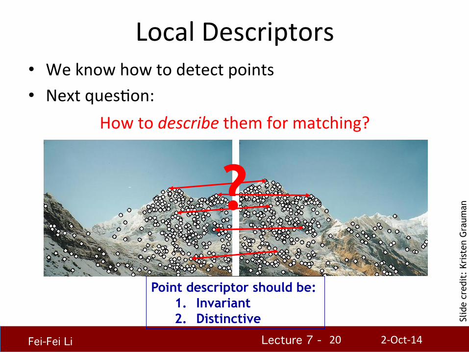
Local Descriptors • We know how to detect points • Next quesHon:
How to describe them for matching?
? Point descriptor should be:
1. Invariant 2. Distinctive Sl
ide
cred
it:
Kris
ten
Gra
uman
2-‐Oct-‐14 20
Lecture 7 - !!!
Fei-Fei Li!
CVPR 2003 Tutorial
Recogni5on and Matching Based on Local Invariant Features
David Lowe Computer Science Department University of BriHsh Columbia
2-‐Oct-‐14 21
Lecture 7 - !!!
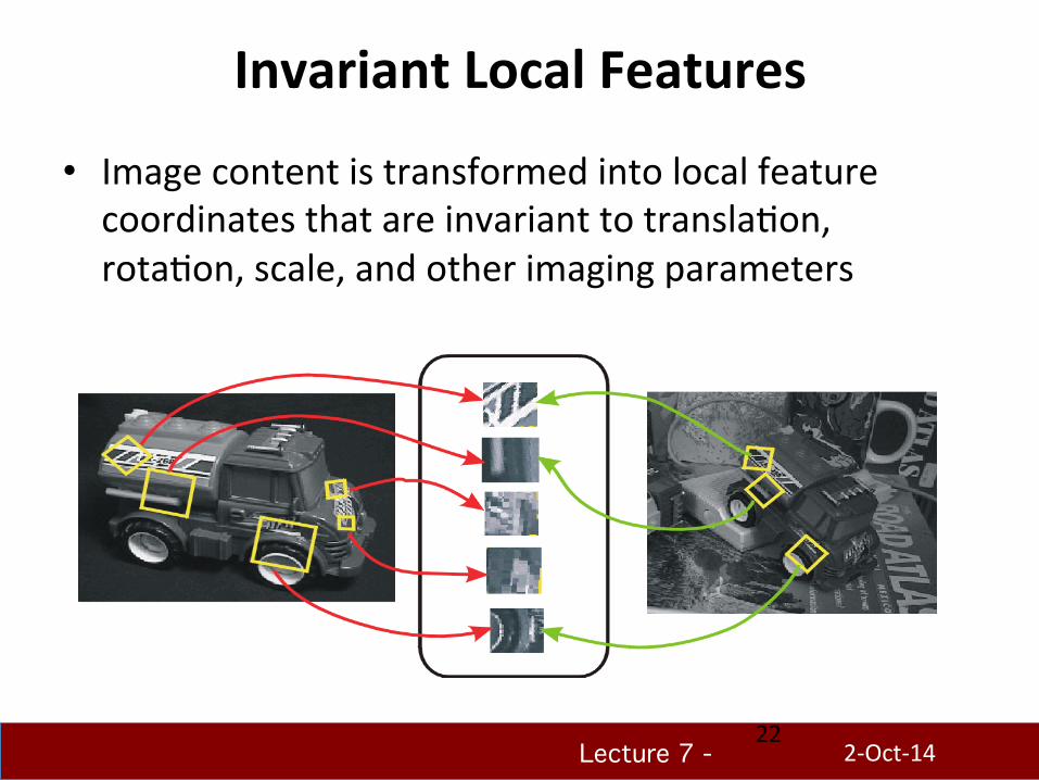
Invariant Local Features
• Image content is transformed into local feature coordinates that are invariant to translaHon, rotaHon, scale, and other imaging parameters
2-‐Oct-‐14 22
Lecture 7 - !!!
Fei-Fei Li!
Advantages of invariant local features • Locality: features are local, so robust to occlusion and cluoer (no prior segmentaHon)
• Dis5nc5veness: individual features can be matched to a large database of objects
• Quan5ty: many features can be generated for even small objects
• Efficiency: close to real-‐Hme performance
• Extensibility: can easily be extended to wide range of differing feature types, with each adding robustness
2-‐Oct-‐14 23
Lecture 7 - !!!
Scale invariance Requires a method to repeatably select points in loca5on
and scale: • The only reasonable scale-‐space kernel is a Gaussian
(Koenderink, 1984; Lindeberg, 1994) • An efficient choice is to detect peaks in the difference of
Gaussian pyramid (Burt & Adelson, 1983; Crowley & Parker, 1984 – but examining more scales)
• Difference-‐of-‐Gaussian with constant raHo of scales is a close approximaHon to Lindeberg’s scale-‐normalized Laplacian (can be shown from the heat diffusion equaHon)
Blur
Resample
Subtract
Blur
Resample
Subtract
2-‐Oct-‐14
Lecture 7 - !!!
Fei-Fei Li!
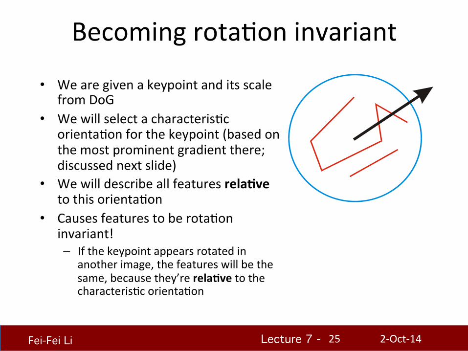
Becoming rotaHon invariant
• We are given a keypoint and its scale from DoG
• We will select a characterisHc orientaHon for the keypoint (based on the most prominent gradient there; discussed next slide)
• We will describe all features rela5ve to this orientaHon
• Causes features to be rotaHon invariant! – If the keypoint appears rotated in
another image, the features will be the same, because they’re rela5ve to the characterisHc orientaHon
0 2π
2-‐Oct-‐14 25
Lecture 7 - !!!
Fei-Fei Li!
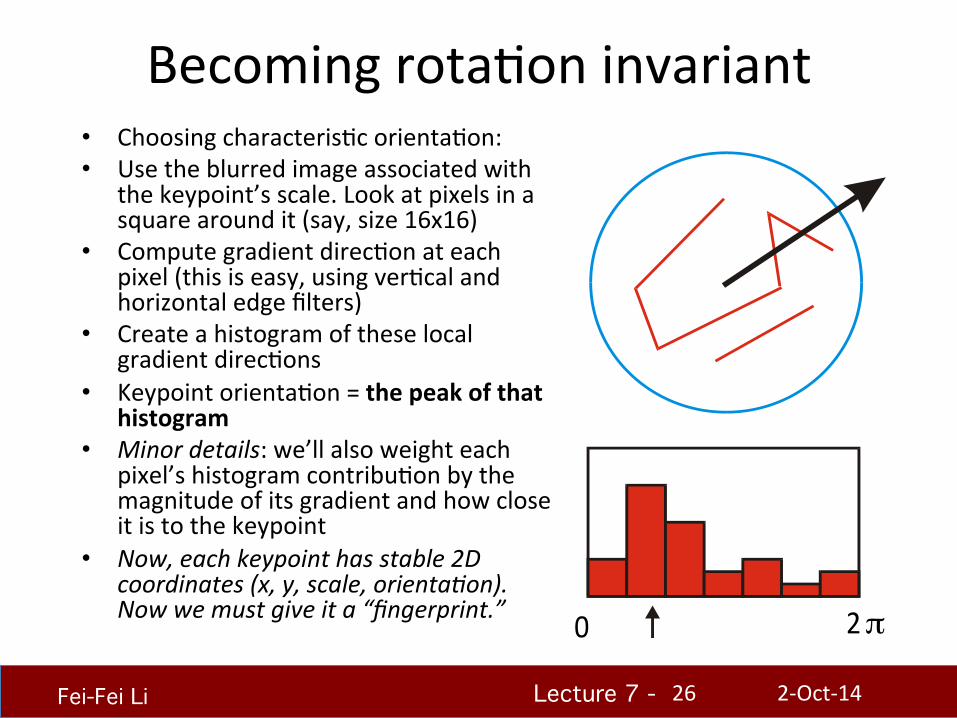
Becoming rotaHon invariant • Choosing characterisHc orientaHon: • Use the blurred image associated with
the keypoint’s scale. Look at pixels in a square around it (say, size 16x16)
• Compute gradient direcHon at each pixel (this is easy, using verHcal and horizontal edge filters)
• Create a histogram of these local gradient direcHons
• Keypoint orientaHon = the peak of that histogram
• Minor details: we’ll also weight each pixel’s histogram contribuHon by the magnitude of its gradient and how close it is to the keypoint
• Now, each keypoint has stable 2D coordinates (x, y, scale, orientaAon). Now we must give it a “fingerprint.” 0 2π
2-‐Oct-‐14 26
Lecture 7 - !!!
Fei-Fei Li!
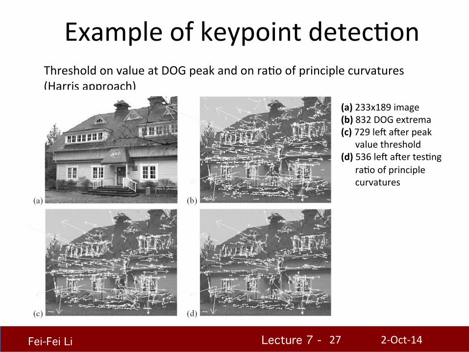
Example of keypoint detecHon Threshold on value at DOG peak and on raHo of principle curvatures (Harris approach)
(a) 233x189 image (b) 832 DOG extrema (c) 729 leu auer peak value threshold (d) 536 leu auer tesHng raHo of principle curvatures
2-‐Oct-‐14 27
Lecture 7 - !!!
Fei-Fei Li!
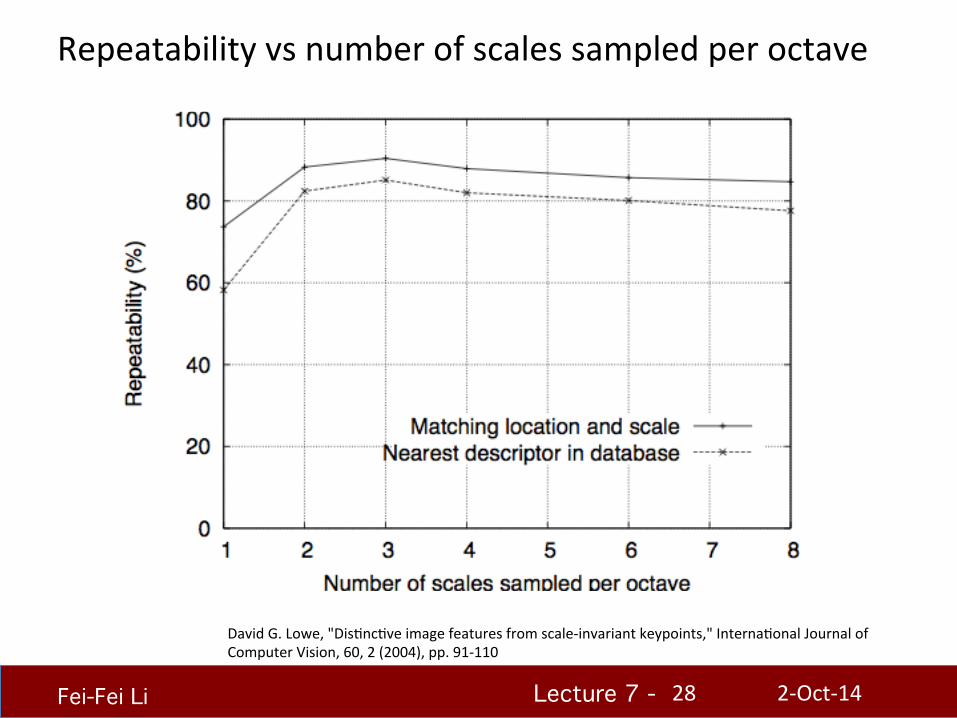
Repeatability vs number of scales sampled per octave
David G. Lowe, "DisHncHve image features from scale-‐invariant keypoints," InternaHonal Journal of Computer Vision, 60, 2 (2004), pp. 91-‐110
2-‐Oct-‐14 28
Lecture 7 - !!!
Fei-Fei Li!
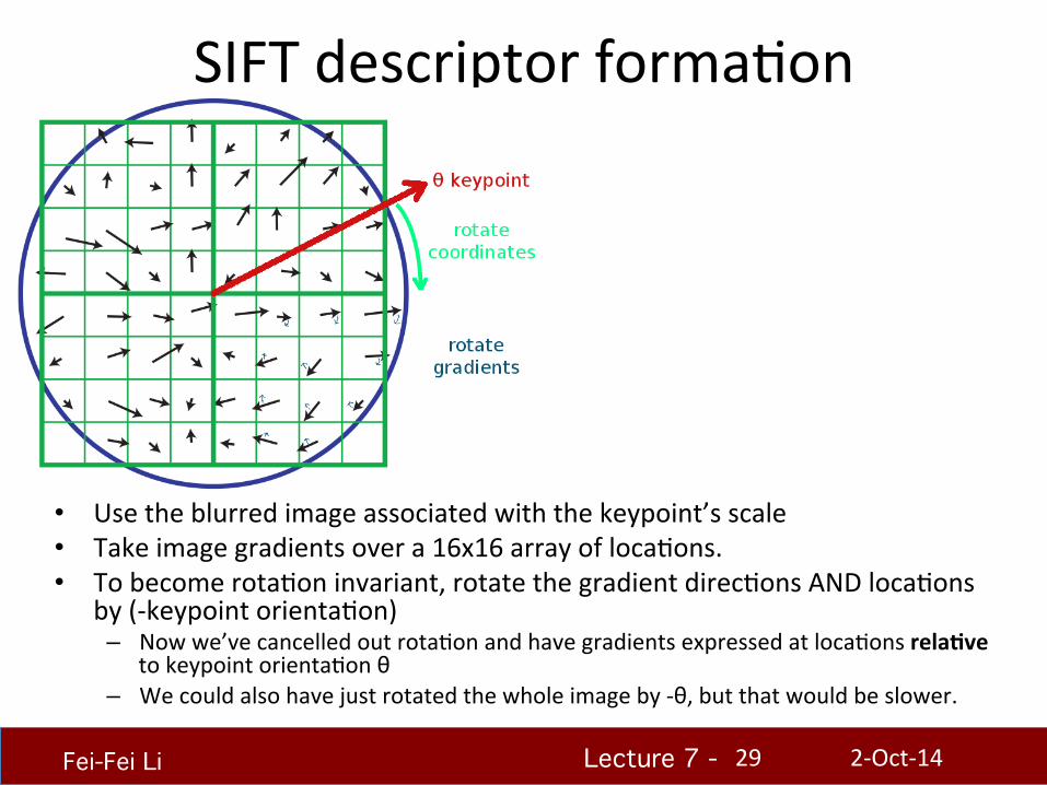
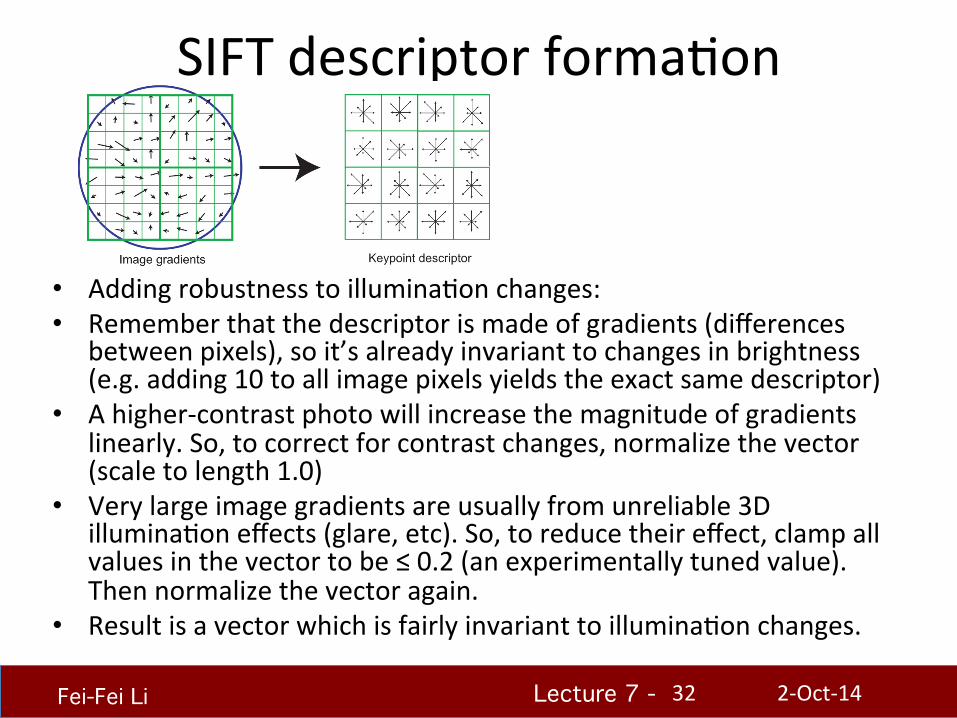
SIFT descriptor formaHon
• Use the blurred image associated with the keypoint’s scale • Take image gradients over a 16x16 array of locaHons. • To become rotaHon invariant, rotate the gradient direcHons AND locaHons
by (-‐keypoint orientaHon) – Now we’ve cancelled out rotaHon and have gradients expressed at locaHons rela5ve
to keypoint orientaHon θ – We could also have just rotated the whole image by -‐θ, but that would be slower.
2-‐Oct-‐14 29

Lecture 7 - !!!
Fei-Fei Li!
SIFT descriptor formaHon
• Using precise gradient locaHons is fragile. We’d like to allow some “slop” in the image, and sHll produce a very similar descriptor
• Create array of orientaHon histograms (a 4x4 array is shown) • Put the rotated gradients into their local orientaHon histograms
– A gradients’s contribuHon is divided among the nearby histograms based on distance. If it’s halfway between two histogram locaHons, it gives a half contribuHon to both.
– Also, scale down gradient contribuHons for gradients far from the center • The SIFT authors found that best results were with 8 orientaHon bins per
histogram, and a 4x4 histogram array.
2-‐Oct-‐14 30
Lecture 7 - !!!
Fei-Fei Li!
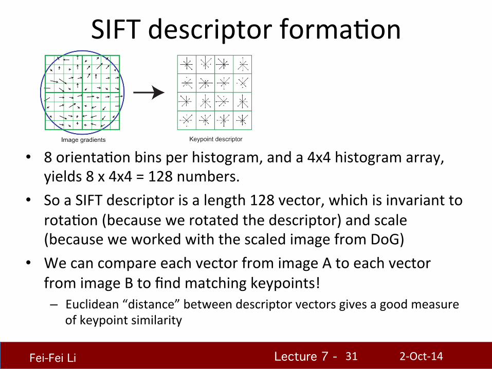
SIFT descriptor formaHon
• 8 orientaHon bins per histogram, and a 4x4 histogram array, yields 8 x 4x4 = 128 numbers.
• So a SIFT descriptor is a length 128 vector, which is invariant to rotaHon (because we rotated the descriptor) and scale (because we worked with the scaled image from DoG)
• We can compare each vector from image A to each vector from image B to find matching keypoints! – Euclidean “distance” between descriptor vectors gives a good measure
of keypoint similarity
2-‐Oct-‐14 31
Lecture 7 - !!!
Fei-Fei Li!
SIFT descriptor formaHon
• Adding robustness to illuminaHon changes: • Remember that the descriptor is made of gradients (differences
between pixels), so it’s already invariant to changes in brightness (e.g. adding 10 to all image pixels yields the exact same descriptor)
• A higher-‐contrast photo will increase the magnitude of gradients linearly. So, to correct for contrast changes, normalize the vector (scale to length 1.0)
• Very large image gradients are usually from unreliable 3D illuminaHon effects (glare, etc). So, to reduce their effect, clamp all values in the vector to be ≤ 0.2 (an experimentally tuned value). Then normalize the vector again.
• Result is a vector which is fairly invariant to illuminaHon changes.
2-‐Oct-‐14 32
Lecture 7 - !!!
Fei-Fei Li!
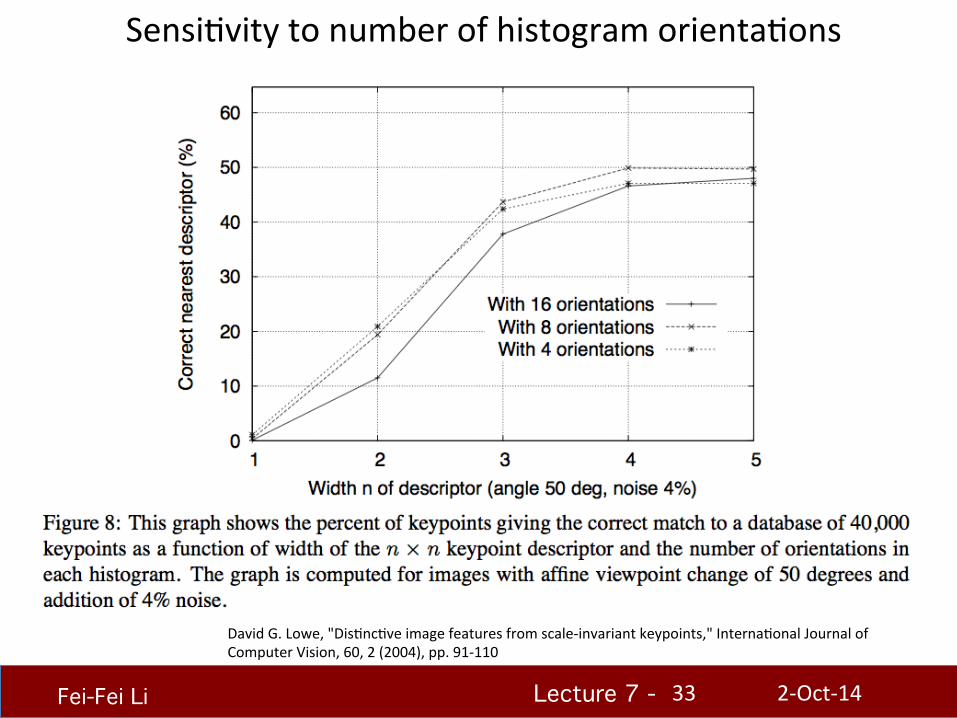
SensiHvity to number of histogram orientaHons
2-‐Oct-‐14 33
David G. Lowe, "DisHncHve image features from scale-‐invariant keypoints," InternaHonal Journal of Computer Vision, 60, 2 (2004), pp. 91-‐110
Lecture 7 - !!!
Fei-Fei Li!
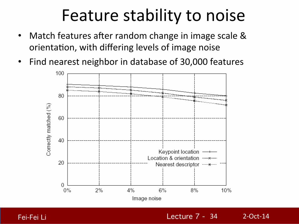
Feature stability to noise • Match features auer random change in image scale &
orientaHon, with differing levels of image noise • Find nearest neighbor in database of 30,000 features
2-‐Oct-‐14 34
Lecture 7 - !!!
Fei-Fei Li!
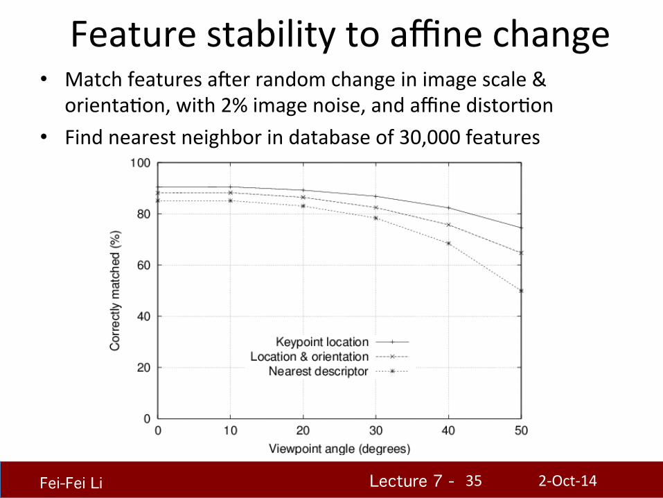
Feature stability to affine change • Match features auer random change in image scale &
orientaHon, with 2% image noise, and affine distorHon • Find nearest neighbor in database of 30,000 features
2-‐Oct-‐14 35
Lecture 7 - !!!
Fei-Fei Li!
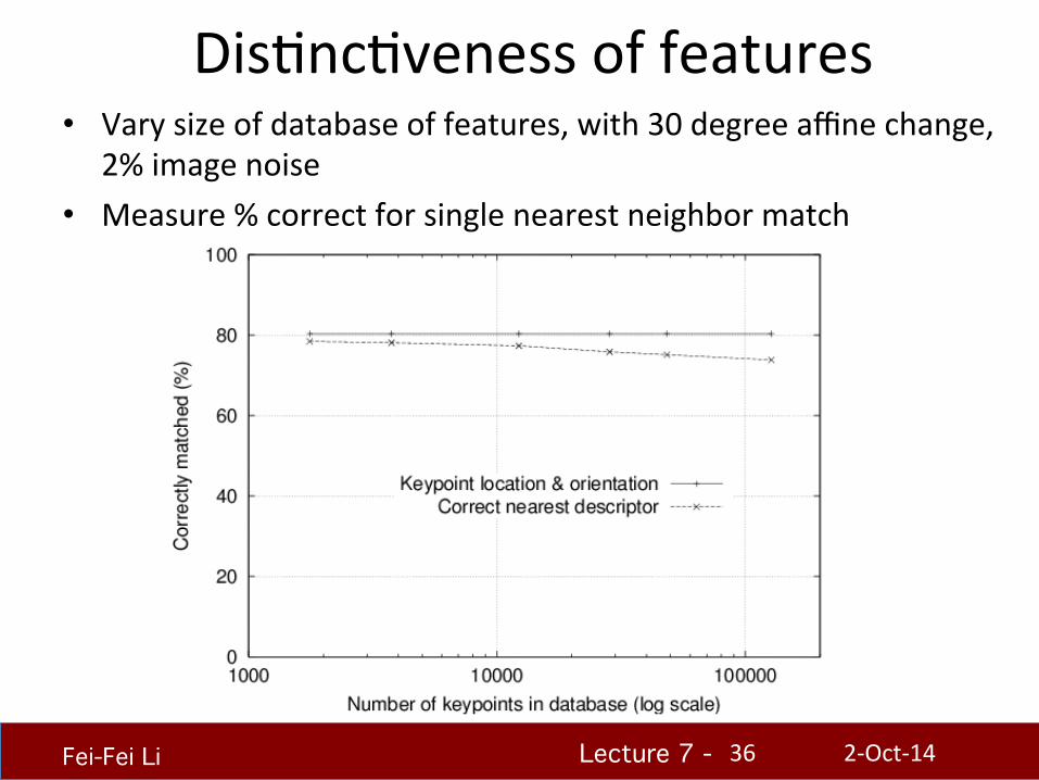
DisHncHveness of features • Vary size of database of features, with 30 degree affine change,
2% image noise • Measure % correct for single nearest neighbor match
2-‐Oct-‐14 36
Lecture 7 - !!!
Fei-Fei Li!
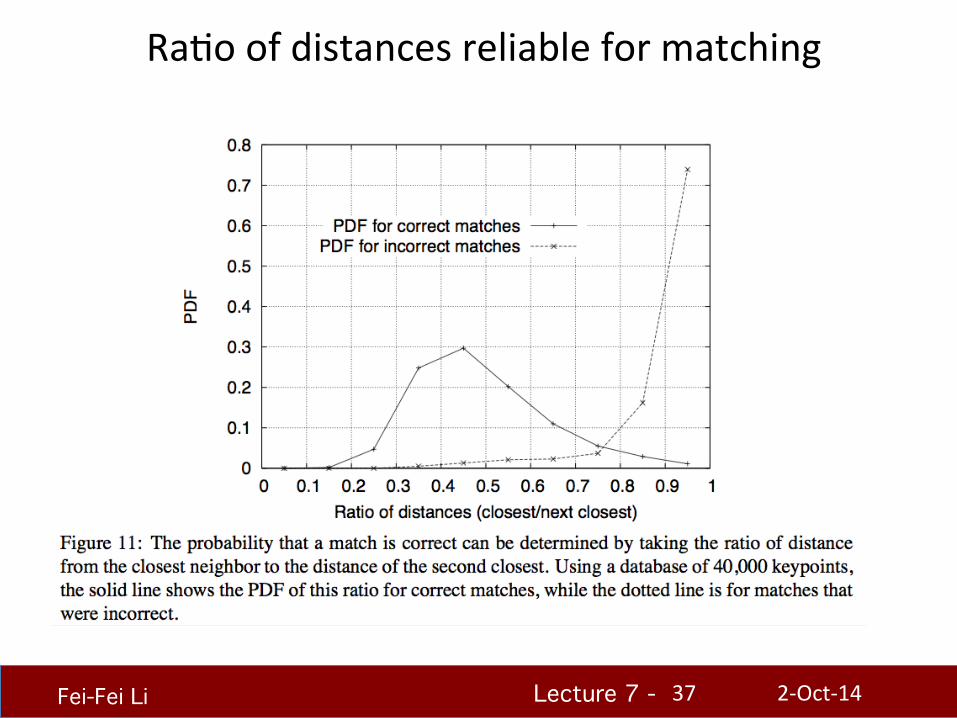
RaHo of distances reliable for matching
2-‐Oct-‐14 37
Lecture 7 - !!!
Fei-Fei Li! 2-‐Oct-‐14 38
Lecture 7 - !!!
Fei-Fei Li! 2-‐Oct-‐14 39
Lecture 7 - !!!
Fei-Fei Li!
Nice SIFT resources
• VLFeat toolbox: – hop://www.vlfeat.org/overview/siu.html
• an online tutorial:hop://www.aishack.in/2010/05/siu-‐scale-‐invariant-‐feature-‐transform/
• Wikipedia:hop://en.wikipedia.org/wiki/Scale-‐invariant_feature_transform
2-‐Oct-‐14 40
Lecture 7 - !!!
Fei-Fei Li!
ApplicaHons of local invariant features
• Wide baseline stereo • MoHon tracking • Panoramas • Mobile robot navigaHon • 3D reconstrucHon • RecogniHon • …

Lecture 7 - !!!
Fei-Fei Li!
AutomaHc mosaicing
hop://www.cs.ubc.ca/~mbrown/autosHtch/autosHtch.html
Lecture 7 - !!!
Fei-Fei Li!
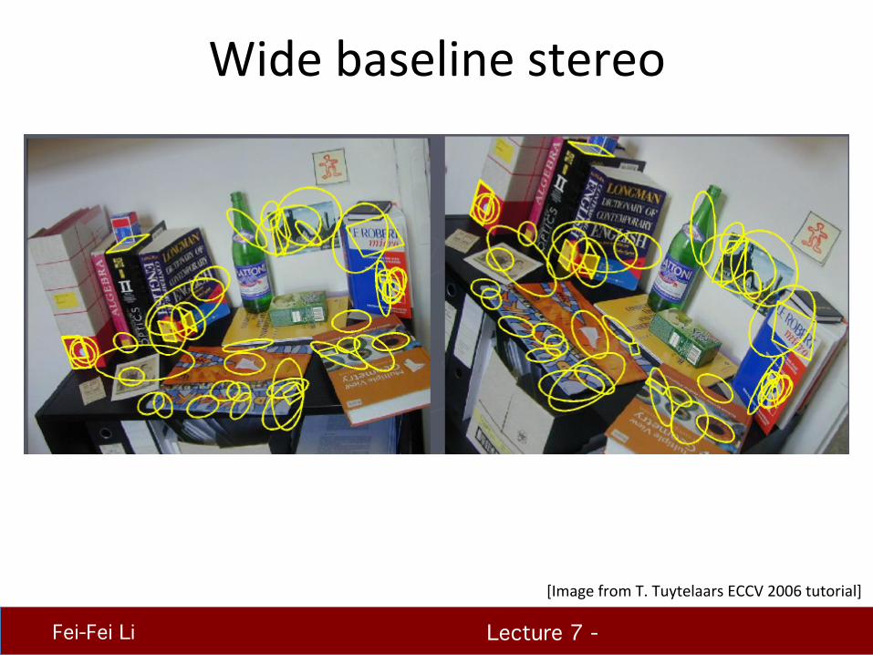
Wide baseline stereo
[Image from T. Tuytelaars ECCV 2006 tutorial]
Lecture 7 - !!!
Fei-Fei Li!
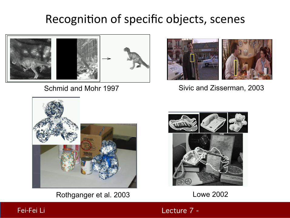
RecogniHon of specific objects, scenes
Rothganger et al. 2003 Lowe 2002
Schmid and Mohr 1997 Sivic and Zisserman, 2003
Lecture 7 - !!!
Fei-Fei Li!
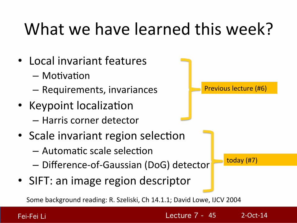
What we have learned this week?
• Local invariant features – MoHvaHon – Requirements, invariances
• Keypoint localizaHon – Harris corner detector
• Scale invariant region selecHon – AutomaHc scale selecHon – Difference-‐of-‐Gaussian (DoG) detector
• SIFT: an image region descriptor
2-‐Oct-‐14 45
Previous lecture (#6)
today (#7)
Some background reading: R. Szeliski, Ch 14.1.1; David Lowe, IJCV 2004