Paper 1339-2017

Interrupted Time Series Power Calculation using DO Loop Simulations

Nigel L. Rozario, Charity G. Moore and Andy McWilliams, CORE-CHS/UNCC

ABSTRACT

Interrupted time series analysis (ITS) is a statistical method that uses repeated “snap shots” over regular time intervals to evaluate healthcare interventions in settings where randomization is not feasible. This method can be used to evaluate programs aimed at improving patient outcomes in real-world, clinical settings. In practice, the number of patients and the timing of observations are restricted. This paper describes a statistical program, which will help statisticians identify optimal time segments within a fixed population size for an interrupted time series analysis. This program creates simulations using “DO loops” to calculate the power needed to detect changes over time that may be due to the interventions under evaluation. Parameters used in this program are total sample size in each time period, number of time periods, and the rate of the event before and after the intervention. The program gives the user the ability to specify different assumptions about these parameters and to assess the resultant power. The output from the program can help statisticians communicate to stakeholders the optimal evaluation design.

INTRODUCTION

Definition of ITS

Interrupted time series (ITS) is a statistical tool for detecting if a policy or intervention has a greater effect than an underlying secular trend, when a randomized trial design is not feasible (Ramsay et al, 2003). Ideally, ITS is used when outcomes can be evaluated using data collected for other purposes, such as administrative data or electronic medical records. Data are collected at multiple time points equally spread before and after an intervention. Additionally, the data requires valid repeated measures and outcomes collected at short time intervals. The analysis entails an autoregressive form of segmented regression analysis to analyze the interrupted time series data (Wagner et al, 2002).

𝑌𝑡 = 𝛽0 + 𝛽1 ∗ 𝑡𝑖𝑚𝑒𝑡 + 𝛽2 ∗ 𝑖𝑛𝑡𝑒𝑟𝑣𝑒𝑛𝑡𝑖𝑜𝑛𝑡 + 𝛽3 ∗ 𝑡𝑖𝑚𝑒 𝑎𝑓𝑡𝑒𝑟 𝑖𝑛𝑡𝑒𝑟𝑣𝑒𝑛𝑡𝑖𝑜𝑛𝑡 + 𝑒𝑡 (Wagner et al, 2002)

In the above equation Yt is the average event rate (e.g. rates of 30-day readmission), which is a dependent variable, while independent variables are time as a continuous variable, intervention indicator (no intervention, intervention), and “time after intervention,” as a continuous variable that counts the number of time units after the intervention is implemented.

As an example, ITS analysis has been used by Du et al to detect whether the addition of a black boxed warning label of suicidal thinking on atomoxetine was associated with a change in prescribing patterns for this Attention Deficit Hyperactivity Disorder (ADHD) medication. The population included patients with an ADHD diagnosis who were prescribed either atomoxetine or stimulants, during January 2004 to December 2007 from the IMC LifeLink Health Plan Claims database. The authors discovered that adults were three times more likely to use atomoxetine than children aged 12 years or younger. An analysis stratified on age showed that the impact of the black box warning differed among the age groups of 12 years and younger, 13 to 18 years, and 18 years and over age groups (Du et al, 2012)

ITS designs allow the investigator to test not only the change in level (β2) but the change in slope of an outcome (β3) which is associated with change in policy or intervention. The method can also be used to assess the unintended consequences of intervention and policy changes through evaluation of other

outcomes. Additionally, it can be used to conduct stratified analysis to evaluate the differential impact of a policy change or intervention on sub populations. (Penfold and Zhang, 2013; Du et al., 2012). For example, in the study by Du et al (2012), a stratified analysis on age showed that the impact of the black box warning differed among age groups of 12 years and younger, 13 to 18 years, and 18 years and over age groups.

There are also a few limitations on applying ITS analysis. They include having at least 8 observation pre as well as post intervention for sufficient power. Also even when there exists a control population randomization is not employed, which leaves a significant chance for bias. Finally, inferences cannot be made on the individual level outcomes when the time series outcomes is looking at population rates (Penfold and Zhang, 2013).

Statisticians working with healthcare leaders often encounter the question of how to best evaluate the implementation of an intervention. From a study validity perspective, a pre/post design has major limitations due to secular trends, regression to the mean, and confounding. Conversely, the ITS design adds additional rigor with the inclusion of multiple time points pre and post intervention, thus testing for linear trends before and after intervention implementation, which may also be compared to trends within a contemporaneous control group. A minimum of 12 data points before intervention and 12 after intervention was suggested by Wagner et al. (2002), not for purposes of power but to adequately evaluate seasonal variation. Penfold and Zhang (2013) indicate that a minimum of 8 observations before and after the intervention are needed to have sufficient power to estimate the regression. A methodologist must balance the desire for multiple observations with the reality that too many segments within a fixed number of patients could result in small patient numbers compromising the stability of the estimates. For example, if 1000 patients are seen during 1 year, we could “slice” the time points 4 times, providing n=250 per period or 10 times, providing n=100 per period. We sought to have a tool available that allowed us to quickly determine the optimal ITS parameters with a given number of patients per time period regardless of the population being studied. As an example, the study that prompted the creation of this simulation pertained to implementing a transition program for patients being discharged from the hospital after a chronic obstructive pulmonary disease (COPD) exacerbation with the intention of decreasing rates of 30-day readmissions.

Impact of n per time period and # of time periods

The main purpose of this simulation exercise is to determine the design parameters for an interrupted time series analysis that will optimize power for testing effectiveness of an intervention. Simulations were created to assess the power to detect a change in outcome immediately after the intervention and in the deviation of the slope of the outcome during the post intervention period.

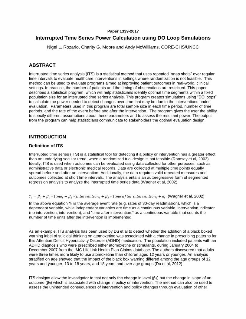
Figure 1: Simulation scenario for readmission rate with time

As an example, Figure 1 shows the simulated readmission rates for N=2000 patients with eight intervals before and after intervention deployment with a resulting sample size of 250 patients per interval. 30% of patients had a 30-dayreadmission before the intervention while 20% of subjects had the event after intervention, suggesting an immediate drop in the rate. In addition, the slope of improvement continues over the next 7 periods demonstrates a continued decline in the event rate to just over 10%. “Time After” is counted only after the intervention. Power for detecting the intervention effect is calculated by simulating the random rates per interval then statistical testing of the coefficients from an autoregressive model and determining the proportion of simulated sets where the null hypothesis is rejected for testing β2 and β3.Two hypotheses are being tested. Firstly, whether the decrease in the event rate is significant comparing pre- and post-intervention (intervention effect). Secondly, whether the slope comparing the pre-intervention trend line is significantly different from the post-intervention trend line.

RESULTS/PROGRAMMING

- Part 1: Data Step

All the analysis in this paper was done using SAS Enterprise Guide® software version 6.1.

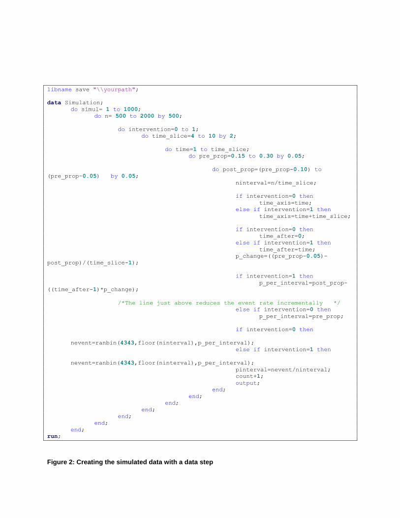
Below is the programming (Figure 2) which is used for the simulation using the do loop. This data step creates 1000 scenarios in which the following parameters are varied: Sample size in the pre and post period is the same (Npre or post=500, 1000, 1500, 2000) and the probability of the event before (pre_prop=0.15, 0.20, 0.25, 0.30) and after (post_prop=pre_prop-0.10). The number of intervals before and after (time_slice) has been varied from 4 to 10, including slightly below and above the number suggested by Penfold and Zhang (2013).

Simulation Parameters

Simul – the number of datasets simulated

N- Sample size for either the pre-intervention (or post-intervention) period

Intervention – Indicator for intervention (0=no, 1=yes)

Pre_Prop – Event rate before the intervention

Post_Prop – Event rate after the intervention

Time_Slice – Number of intervals for the time period divided before or after

Nevent – Number of people having the event generated from a random binomial distribution with N/Time_Slice as sample size pre_prop or post_prop as the population event rate

Time_Axis – The count of the number of time points during the pre or post period (e.g. Time Slice of 4 would have four time points for pre- and post)

Time_After – Time points after the intervention

Pinterval – Probability of the event with time (which may decrease or stay the same with time)

libname save "\\yourpath";

data Simulation;

do simul= 1 to 1000;

do n= 500 to 2000 by 500;

do intervention=0 to 1;

do time_slice=4 to 10 by 2;

do time=1 to time_slice;

do pre_prop=0.15 to 0.30 by 0.05;

do post_prop=(pre_prop-0.10) to

(pre_prop-0.05) by 0.05;

ninterval=n/time_slice;

if intervention=0 then

time_axis=time;

else if intervention=1 then

time_axis=time+time_slice;

if intervention=0 then

time_after=0;

else if intervention=1 then

time_after=time;

p_change=((pre_prop-0.05)-

post_prop)/(time_slice-1);

if intervention=1 then

p_per_interval=post_prop-

((time_after-1)*p_change);

/*The line just above reduces the event rate incrementally */

else if intervention=0 then

p_per_interval=pre_prop;

if intervention=0 then

nevent=ranbin(4343,floor(ninterval),p_per_interval);

else if intervention=1 then

nevent=ranbin(4343,floor(ninterval),p_per_interval);

pinterval=nevent/ninterval;

count+1;

output;

end;

end;

end;

end;

end;

end;

end;

run;

Figure 2: Creating the simulated data with a data step

- Part 2: PROC SORT and PROC AUTOREG

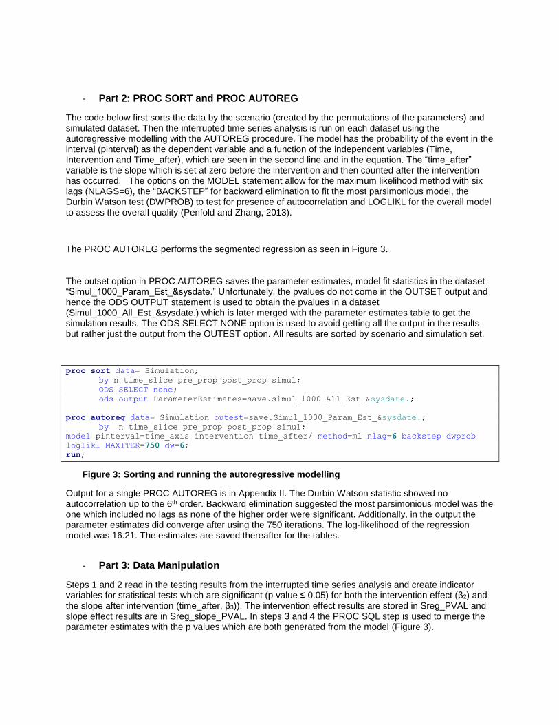
The code below first sorts the data by the scenario (created by the permutations of the parameters) and simulated dataset. Then the interrupted time series analysis is run on each dataset using the autoregressive modelling with the AUTOREG procedure. The model has the probability of the event in the interval (pinterval) as the dependent variable and a function of the independent variables (Time, Intervention and Time_after), which are seen in the second line and in the equation. The “time_after” variable is the slope which is set at zero before the intervention and then counted after the intervention has occurred. The options on the MODEL statement allow for the maximum likelihood method with six lags (NLAGS=6), the “BACKSTEP” for backward elimination to fit the most parsimonious model, the Durbin Watson test (DWPROB) to test for presence of autocorrelation and LOGLIKL for the overall model to assess the overall quality (Penfold and Zhang, 2013).

The PROC AUTOREG performs the segmented regression as seen in Figure 3.

The outset option in PROC AUTOREG saves the parameter estimates, model fit statistics in the dataset “Simul_1000_Param_Est_&sysdate.” Unfortunately, the pvalues do not come in the OUTSET output and hence the ODS OUTPUT statement is used to obtain the pvalues in a dataset (Simul_1000_All_Est_&sysdate.) which is later merged with the parameter estimates table to get the simulation results. The ODS SELECT NONE option is used to avoid getting all the output in the results but rather just the output from the OUTEST option. All results are sorted by scenario and simulation set.

proc sort data= Simulation;

by n time_slice pre_prop post_prop simul;

ODS SELECT none;

ods output ParameterEstimates=save.simul_1000_All_Est_&sysdate.;

proc autoreg data= Simulation outest=save.Simul_1000_Param_Est_&sysdate.;

by n time_slice pre_prop post_prop simul;

model pinterval=time_axis intervention time_after/ method=ml nlag=6 backstep dwprob

loglikl MAXITER=750 dw=6;

run;

Figure 3: Sorting and running the autoregressive modelling

Output for a single PROC AUTOREG is in Appendix II. The Durbin Watson statistic showed no autocorrelation up to the 6th order. Backward elimination suggested the most parsimonious model was the one which included no lags as none of the higher order were significant. Additionally, in the output the parameter estimates did converge after using the 750 iterations. The log-likelihood of the regression model was 16.21. The estimates are saved thereafter for the tables.

- Part 3: Data Manipulation

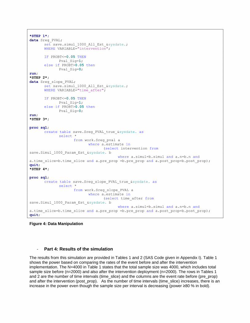
Steps 1 and 2 read in the testing results from the interrupted time series analysis and create indicator variables for statistical tests which are significant (p value ≤ 0.05) for both the intervention effect (β2) and the slope after intervention (time_after, β3)). The intervention effect results are stored in Sreg_PVAL and slope effect results are in Sreg_slope_PVAL. In steps 3 and 4 the PROC SQL step is used to merge the parameter estimates with the p values which are both generated from the model (Figure 3).

*STEP 1*;

data Sreg_PVAL;

set save.simul_1000_All_Est_&sysdate.;

WHERE VARIABLE="intervention";

IF PROBT<=0.05 THEN

Pval_Sig=1;

else if PROBT>0.05 then

Pval_Sig=0;

run;

*STEP 2*;

data Sreg_slope_PVAL;

set save.simul_1000_All_Est_&sysdate.;

WHERE VARIABLE="time_after";

IF PROBT<=0.05 THEN

Pval_Sig=1;

else if PROBT>0.05 then

Pval_Sig=0;

run;

*STEP 3*;

proc sql;

create table save.Sreg_PVAL_true_&sysdate. as

select *

from work.Sreg_pval a

where a.estimate in

(select intervention from

save.Simul_1000_Param_Est_&sysdate. b

where a.simul=b.simul and a.n=b.n and

a.time_slice=b.time_slice and a.pre_prop =b.pre_prop and a.post_prop=b.post_prop);

quit;

*STEP 4*;

proc sql;

create table save.Sreg_slope_PVAL_true_&sysdate. as

select *

from work.Sreg_slope_PVAL a

where a.estimate in

(select time_after from

save.Simul_1000_Param_Est_&sysdate. b

where a.simul=b.simul and a.n=b.n and

a.time_slice=b.time_slice and a.pre_prop =b.pre_prop and a.post_prop=b.post_prop);

quit;

Figure 4: Data Manipulation

- Part 4: Results of the simulation

The results from this simulation are provided in Tables 1 and 2 (SAS Code given in Appendix I). Table 1 shows the power based on comparing the rates of the event before and after the intervention implementation. The N=4000 in Table 1 states that the total sample size was 4000, which includes total sample size before (n=2000) and also after the intervention deployment (n=2000). The rows in Tables 1 and 2 are the number of time intervals (time_slice) and the columns are the event rate before (pre_prop) and after the intervention (post_prop). As the number of time intervals (time_slice) increases, there is an increase in the power even though the sample size per interval is decreasing (power ≥80 % in bold).

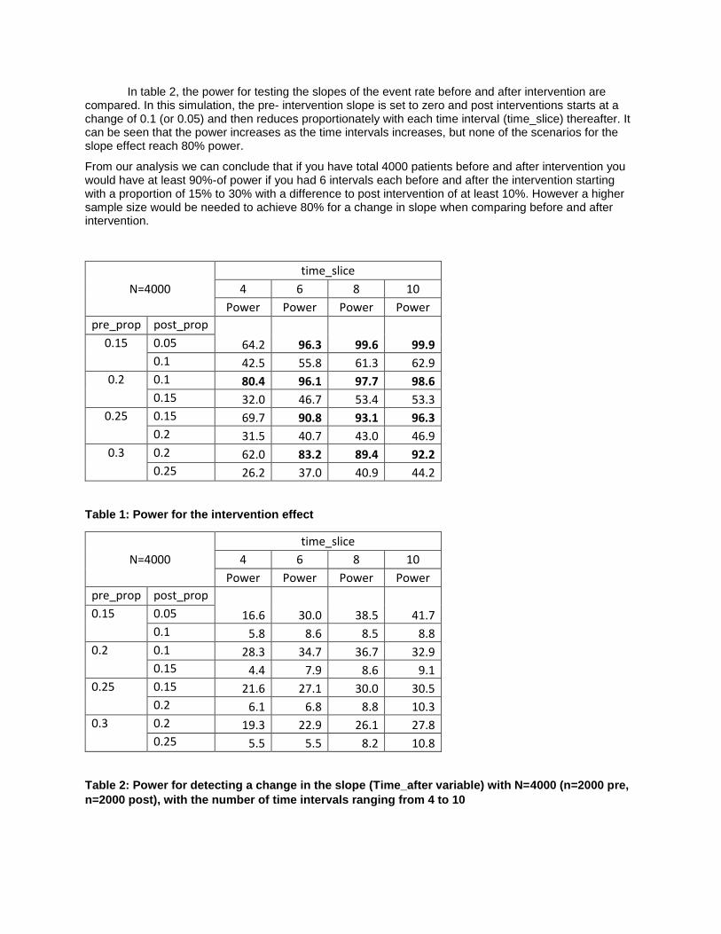
In table 2, the power for testing the slopes of the event rate before and after intervention are compared. In this simulation, the pre- intervention slope is set to zero and post interventions starts at a change of 0.1 (or 0.05) and then reduces proportionately with each time interval (time_slice) thereafter. It can be seen that the power increases as the time intervals increases, but none of the scenarios for the slope effect reach 80% power.

From our analysis we can conclude that if you have total 4000 patients before and after intervention you would have at least 90%-of power if you had 6 intervals each before and after the intervention starting with a proportion of 15% to 30% with a difference to post intervention of at least 10%. However a higher sample size would be needed to achieve 80% for a change in slope when comparing before and after intervention.

N=4000

time_slice

4 6 8 10

Power Power Power Power

pre_prop post_prop

64.2 96.3 99.6 99.9 0.15 0.05

0.1 42.5 55.8 61.3 62.9

0.2 0.1 80.4 96.1 97.7 98.6

0.15 32.0 46.7 53.4 53.3

0.25 0.15 69.7 90.8 93.1 96.3

0.2 31.5 40.7 43.0 46.9

0.3 0.2 62.0 83.2 89.4 92.2

0.25 26.2 37.0 40.9 44.2

Table 1: Power for the intervention effect

N=4000

time_slice

4 6 8 10

Power Power Power Power

pre_prop post_prop

16.6 30.0 38.5 41.7 0.15 0.05

0.1 5.8 8.6 8.5 8.8

0.2 0.1 28.3 34.7 36.7 32.9

0.15 4.4 7.9 8.6 9.1

0.25 0.15 21.6 27.1 30.0 30.5

0.2 6.1 6.8 8.8 10.3

0.3 0.2 19.3 22.9 26.1 27.8

0.25 5.5 5.5 8.2 10.8

Table 2: Power for detecting a change in the slope (Time_after variable) with N=4000 (n=2000 pre,

n=2000 post), with the number of time intervals ranging from 4 to 10

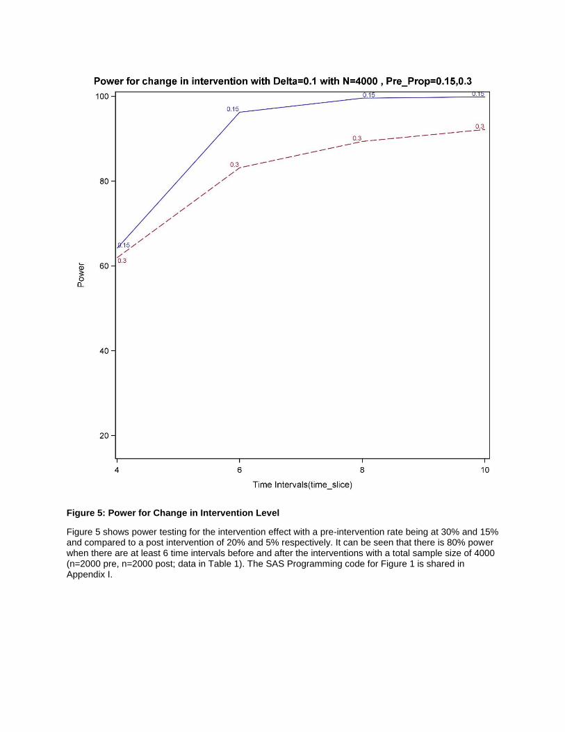
Figure 5: Power for Change in Intervention Level

Figure 5 shows power testing for the intervention effect with a pre-intervention rate being at 30% and 15% and compared to a post intervention of 20% and 5% respectively. It can be seen that there is 80% power when there are at least 6 time intervals before and after the interventions with a total sample size of 4000 (n=2000 pre, n=2000 post; data in Table 1). The SAS Programming code for Figure 1 is shared in Appendix I.

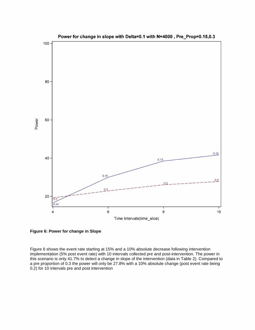
Figure 6: Power for change in Slope

Figure 6 shows the event rate starting at 15% and a 10% absolute decrease following intervention implementation (5% post event rate) with 10 intervals collected pre and post-intervention. The power in this scenario is only 41.7% to detect a change in slope of the intervention (data in Table 2). Compared to a pre proportion of 0.3 the power will only be 27.8% with a 10% absolute change (post event rate being 0.2) for 10 intervals pre and post intervention

CONCLUSION

ITS has a good graphical and numerical presentation which can be well understood by an audience with minimal knowledge of epidemiological and statistical methods. (Bernal, Cummins & Gasparrini, 2016). We have developed a tool that will allow us to easily test different scenarios regardless of the type of outcome, total sample size, and time period for study using ITS. We can quickly assess if it is realistic to propose an interrupted time series analysis to test if a programmatic or policy level intervention had an effect, even for studies where the total sample sizes may be smaller particularly for certain disease populations.

REFERENCES:

Hemming, K., & Taljaard, M. (2016). Sample size calculations for stepped wedge and cluster randomised

trials: a unified approach. Journal of clinical epidemiology, 69, 137-146.

Penfold, R. B., & Zhang, F. (2013). Use of interrupted time series analysis in evaluating health care

quality improvements. Academic pediatrics, 13(6), S38-S44.

Ramsey, C. R., Matowe, L., Grilli, R., Grimshaw, J. M., & Thomas, R. E. (2003). Interrupted time series

designs in health technology assessment: lessons from two systematic reviews of behaviour change

strategies. Int J Technol Assess Health Care, 19(4), 613-623.

Biglan, A., Ary, D., & Wagenaar, A. C. (2000). The value of interrupted time-series experiments for

community intervention research. Prevention Science, 1(1), 31-49.

Du, D. T., Zhou, E. H., Goldsmith, J., Nardinelli, C., & Hammad, T. A. (2012). Atomoxetine use during a

period of FDA actions. Medical care, 50(11), 987-992.

Wagner, A. K., Soumerai, S. B., Zhang, F., & Ross‐Degnan, D. (2002). Segmented regression analysis of

interrupted time series studies in medication use research. Journal of clinical pharmacy and

therapeutics, 27(4), 299-309.

Bernal, J. L., Cummins, S., & Gasparrini, A. (2016). Interrupted time series regression for the evaluation

of public health interventions: a tutorial. International journal of epidemiology, dyw098.

Bhaskaran, K., Gasparrini, A., Hajat, S., Smeeth, L., & Armstrong, B. (2013). Time series regression

studies in environmental epidemiology. International journal of epidemiology, dyt092.

ACKNOWLEDGMENTS

The authors would like to thank the Center for Outcomes Research and Evaluation Biostatistics team from Carolinas HealthCare System for providing useful feedback for the manuscript.

CONTACT INFORMATION

Your comments and questions are valued and encouraged. Contact the author at:

Nigel L. Rozario, MS CHS-Center for Outcomes Research (CORE) 704-355-0170 nrozario@uncc.edu

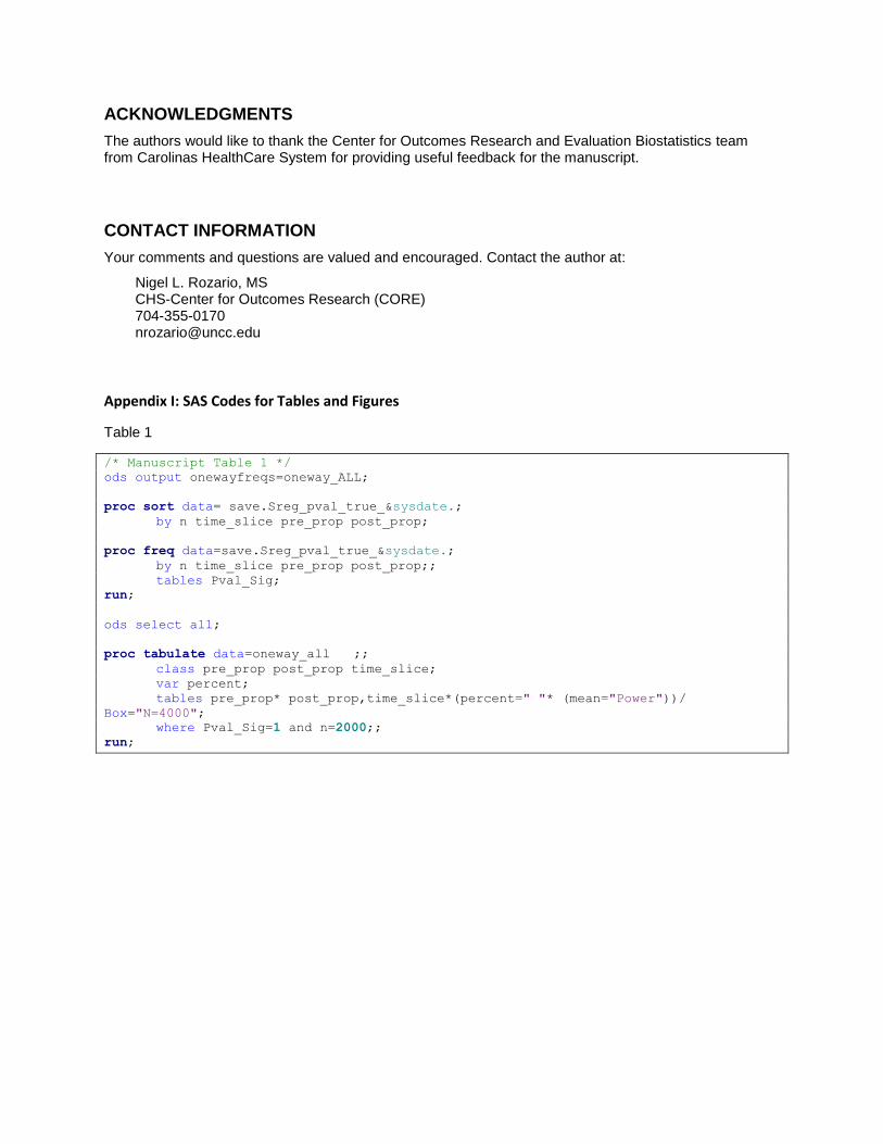
Appendix I: SAS Codes for Tables and Figures

Table 1

/* Manuscript Table 1 */

ods output onewayfreqs=oneway_ALL;

proc sort data= save.Sreg_pval_true_&sysdate.;

by n time_slice pre_prop post_prop;

proc freq data=save.Sreg_pval_true_&sysdate.;

by n time_slice pre_prop post_prop;;

tables Pval_Sig;

run;

ods select all;

proc tabulate data=oneway_all ;;

class pre_prop post_prop time_slice;

var percent;

tables pre_prop* post_prop,time_slice*(percent=" "* (mean="Power"))/

Box="N=4000";

where Pval_Sig=1 and n=2000;;

run;

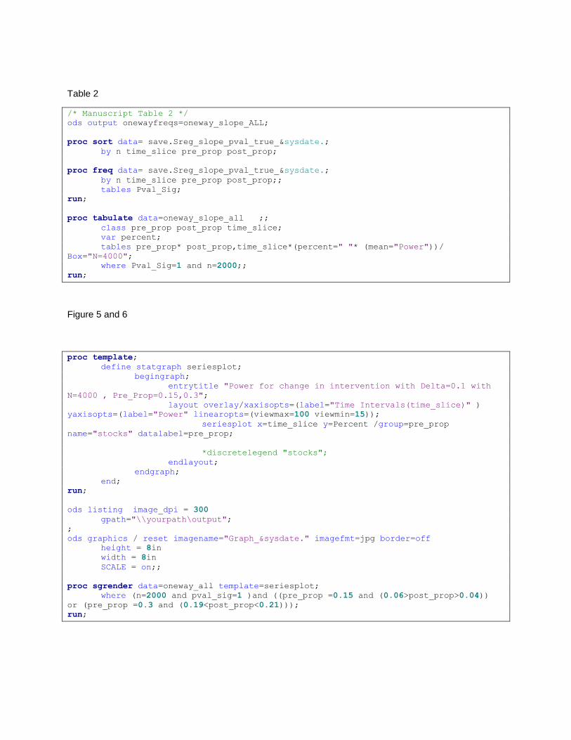
Table 2

/* Manuscript Table 2 */

ods output onewayfreqs=oneway_slope_ALL;

proc sort data= save.Sreg_slope_pval_true_&sysdate.;

by n time_slice pre_prop post_prop;

proc freq data= save.Sreg_slope_pval_true_&sysdate.;

by n time_slice pre_prop post_prop;;

tables Pval_Sig;

run;

proc tabulate data=oneway_slope_all ;;

class pre_prop post_prop time_slice;

var percent;

tables pre_prop* post_prop,time_slice*(percent=" "* (mean="Power"))/

Box="N=4000";

where Pval_Sig=1 and n=2000;;

run;

Figure 5 and 6

proc template;

define statgraph seriesplot;

begingraph;

entrytitle "Power for change in intervention with Delta=0.1 with

N=4000 , Pre_Prop=0.15,0.3";

layout overlay/xaxisopts=(label="Time Intervals(time_slice)" )

yaxisopts=(label="Power" linearopts=(viewmax=100 viewmin=15));

seriesplot x=time_slice y=Percent /group=pre_prop

name="stocks" datalabel=pre_prop;

*discretelegend "stocks";

endlayout;

endgraph;

end;

run;

ods listing image_dpi = 300

gpath="\\yourpath\output";

;

ods graphics / reset imagename="Graph_&sysdate." imagefmt=jpg border=off

height = 8in

width = 8in

SCALE = on;;

proc sgrender data=oneway_all template=seriesplot;

where (n=2000 and pval_sig=1 )and ((pre_prop =0.15 and (0.06>post_prop>0.04))

or (pre_prop =0.3 and (0.19<post_prop<0.21)));

run;

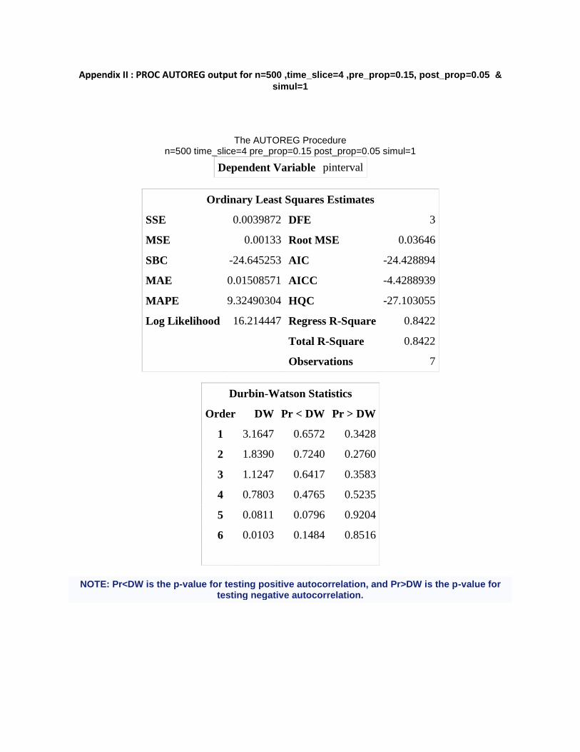
Appendix II : PROC AUTOREG output for n=500 ,time_slice=4 ,pre_prop=0.15, post_prop=0.05 &

simul=1

The AUTOREG Procedure n=500 time_slice=4 pre_prop=0.15 post_prop=0.05 simul=1

Dependent Variable pinterval

Ordinary Least Squares Estimates

SSE 0.0039872 DFE 3

MSE 0.00133 Root MSE 0.03646

SBC -24.645253 AIC -24.428894

MAE 0.01508571 AICC -4.4288939

MAPE 9.32490304 HQC -27.103055

Log Likelihood 16.214447 Regress R-Square 0.8422

Total R-Square 0.8422

Observations 7

Durbin-Watson Statistics

Order DW Pr < DW Pr > DW

1 3.1647 0.6572 0.3428

2 1.8390 0.7240 0.2760

3 1.1247 0.6417 0.3583

4 0.7803 0.4765 0.5235

5 0.0811 0.0796 0.9204

6 0.0103 0.1484 0.8516

NOTE: Pr<DW is the p-value for testing positive autocorrelation, and Pr>DW is the p-value for testing negative autocorrelation.

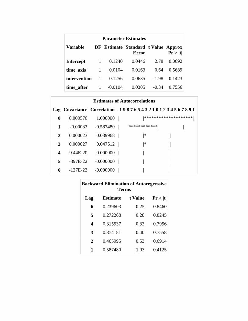
Parameter Estimates

Variable DF Estimate Standard

Error

t Value Approx

Pr > |t|

Intercept 1 0.1240 0.0446 2.78 0.0692

time_axis 1 0.0104 0.0163 0.64 0.5689

intervention 1 -0.1256 0.0635 -1.98 0.1423

time_after 1 -0.0104 0.0305 -0.34 0.7556

Estimates of Autocorrelations

Lag Covariance Correlation -1 9 8 7 6 5 4 3 2 1 0 1 2 3 4 5 6 7 8 9 1

0 0.000570 1.000000 | |********************|

1 -0.00033 -0.587480 | ************| |

2 0.000023 0.039968 | |* |

3 0.000027 0.047512 | |* |

4 9.44E-20 0.000000 | | |

5 -397E-22 -0.000000 | | |

6 -127E-22 -0.000000 | | |

Backward Elimination of Autoregressive

Terms

Lag Estimate t Value Pr > |t|

6 0.239603 0.25 0.8460

5 0.272268 0.28 0.8245

4 0.315537 0.33 0.7956

3 0.374181 0.40 0.7558

2 0.465995 0.53 0.6914

1 0.587480 1.03 0.4125