Interrupted Time Series Designs

Overview

• Role of ITS in the history of WSC

– Two classes of ITS for WSCs

• Two examples of WSC comparing ITS to RE

• Issues in ITS vs RE WSCs

– Methodological and logistical

– Analytical

ITS

• A series of observations on a dependent variable over time

– N = 100 observations is the desirable standard

– N < 100 observations is still helpful, even with very few observations—and by far the most common!

• Interrupted by the introduction of an intervention.

• The time series should show an “effect” at the time of the interruption.

Two Classes of ITS for WSC

• Large scale ITS on aggregates

• Single-case (SCD) and N-of-1 designs in social science and medicine

• These two classes turn out to have very different advantages and disadvantages in the context of WSCs.

• Consider examples of the two classes:

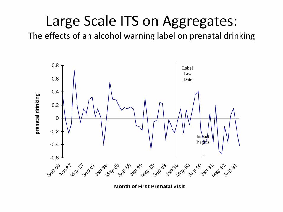
Large Scale ITS on Aggregates: The effects of an alcohol warning label on prenatal drinking

-0.6

-0.4

-0.2

0

0.2

0.4

0.6

0.8

Sep-8

6

Jan-

87

May

-87

Sep-8

7

Jan-

88

May

-88

Sep-8

8

Jan-

89

May

-89

Sep-8

9

Jan-

90

May

-90

Sep-9

0

Jan-

91

May

-91

Sep-9

1

Month of First Prenatal Visit

pre

nata

l d

rin

kin

g

Label

Law

Date

Impact

Begins

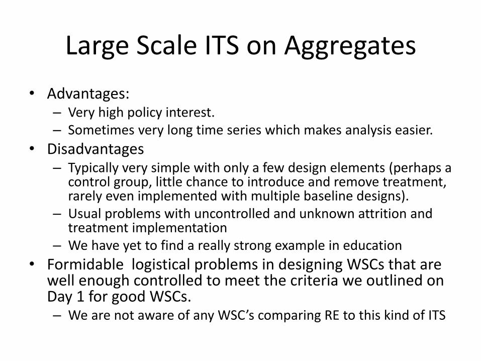
Large Scale ITS on Aggregates

• Advantages: – Very high policy interest. – Sometimes very long time series which makes analysis easier.

• Disadvantages – Typically very simple with only a few design elements (perhaps a

control group, little chance to introduce and remove treatment, rarely even implemented with multiple baseline designs).

– Usual problems with uncontrolled and unknown attrition and treatment implementation

– We have yet to find a really strong example in education

• Formidable logistical problems in designing WSCs that are well enough controlled to meet the criteria we outlined on Day 1 for good WSCs. – We are not aware of any WSC’s comparing RE to this kind of ITS

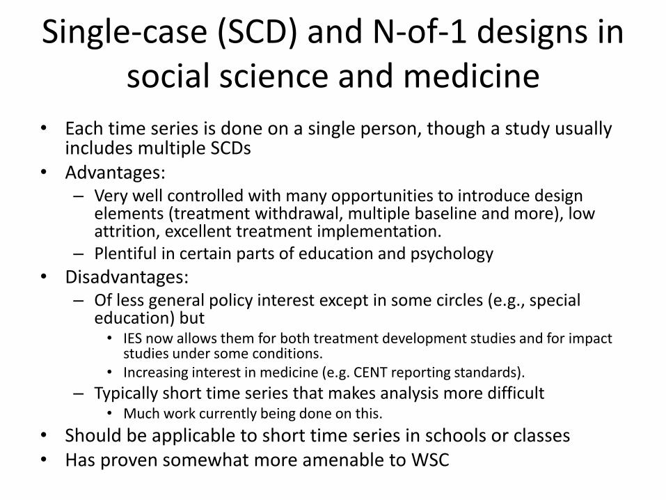
Single-case (SCD) and N-of-1 designs in social science and medicine

• Each time series is done on a single person, though a study usually includes multiple SCDs

• Advantages: – Very well controlled with many opportunities to introduce design

elements (treatment withdrawal, multiple baseline and more), low attrition, excellent treatment implementation.

– Plentiful in certain parts of education and psychology

• Disadvantages: – Of less general policy interest except in some circles (e.g., special

education) but • IES now allows them for both treatment development studies and for impact

studies under some conditions. • Increasing interest in medicine (e.g. CENT reporting standards).

– Typically short time series that makes analysis more difficult • Much work currently being done on this.

• Should be applicable to short time series in schools or classes • Has proven somewhat more amenable to WSC

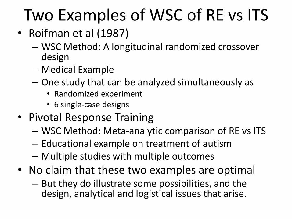
Two Examples of WSC of RE vs ITS • Roifman et al (1987)

– WSC Method: A longitudinal randomized crossover design

– Medical Example – One study that can be analyzed simultaneously as

• Randomized experiment • 6 single-case designs

• Pivotal Response Training – WSC Method: Meta-analytic comparison of RE vs ITS – Educational example on treatment of autism – Multiple studies with multiple outcomes

• No claim that these two examples are optimal – But they do illustrate some possibilities, and the

design, analytical and logistical issues that arise.

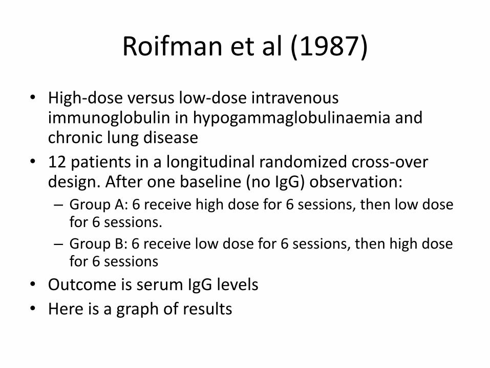
Roifman et al (1987)

• High-dose versus low-dose intravenous immunoglobulin in hypogammaglobulinaemia and chronic lung disease

• 12 patients in a longitudinal randomized cross-over design. After one baseline (no IgG) observation: – Group A: 6 receive high dose for 6 sessions, then low dose

for 6 sessions.

– Group B: 6 receive low dose for 6 sessions, then high dose for 6 sessions

• Outcome is serum IgG levels

• Here is a graph of results

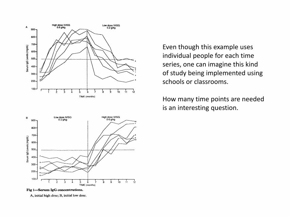
Even though this example uses individual people for each time series, one can imagine this kind of study being implemented using schools or classrooms. How many time points are needed is an interesting question.

Analysis Strategy

• To compare RE to SCD results, we analyze the data two ways – As an N-of-1 Trial: Analyze Group B only as if it

were six single-case designs

– As a RE: Analyze Time 6 data as a randomized experiment comparing Group A and Group B.

• Analyst blinding – I analyzed the RE

– David Rindskopf analyzed SCD

Analytic Methods • The RCT is easy

– usual regression (or ANOVA) to get group mean difference and se. • We did run ANCOVA covarying pretest but results were

essentially the same.

– Or a usual d-statistic (or bias-corrected g)

• The SCD analysis needs to produce a result that is in a comparable metric – Used a multilevel model in WinBUGS to adjust for

nonlinearity and get a group mean difference at time 6 (or 12, but with potential carryover effects)

– d-statistic (or g) for SCD that is in the same metric as the usual between-groups d (Hedges, Pustejovsky & Shadish, in press). • But current incarnation assumes linearity

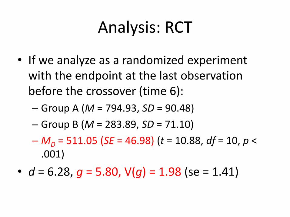
Analysis: RCT

• If we analyze as a randomized experiment with the endpoint at the last observation before the crossover (time 6):

– Group A (M = 794.93, SD = 90.48)

– Group B (M = 283.89, SD = 71.10)

– MD = 511.05 (SE = 46.98) (t = 10.88, df = 10, p < .001)

• d = 6.28, g = 5.80, V(g) = 1.98 (se = 1.41)

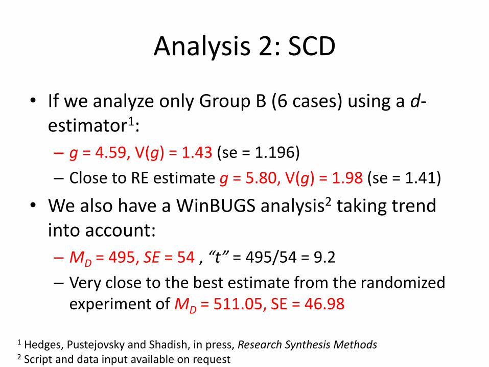
Analysis 2: SCD

• If we analyze only Group B (6 cases) using a d-estimator1:

– g = 4.59, V(g) = 1.43 (se = 1.196)

– Close to RE estimate g = 5.80, V(g) = 1.98 (se = 1.41)

• We also have a WinBUGS analysis2 taking trend into account:

– MD = 495, SE = 54 , “t” = 495/54 = 9.2

– Very close to the best estimate from the randomized experiment of MD = 511.05, SE = 46.98

1 Hedges, Pustejovsky and Shadish, in press, Research Synthesis Methods 2 Script and data input available on request

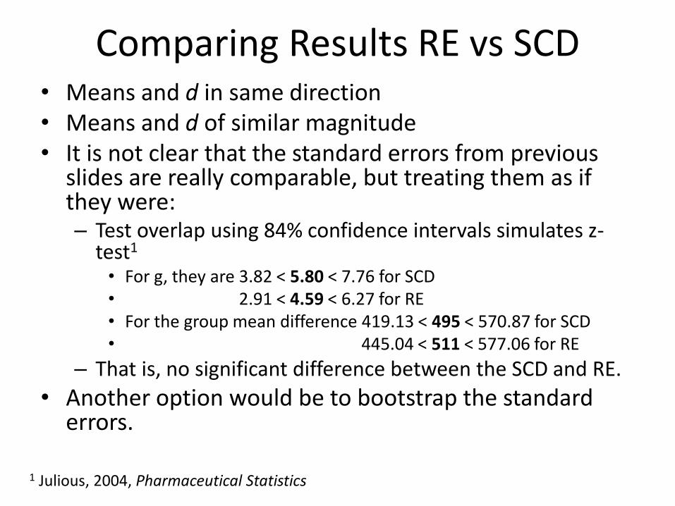
Comparing Results RE vs SCD • Means and d in same direction • Means and d of similar magnitude • It is not clear that the standard errors from previous

slides are really comparable, but treating them as if they were: – Test overlap using 84% confidence intervals simulates z-

test1

• For g, they are 3.82 < 5.80 < 7.76 for SCD • 2.91 < 4.59 < 6.27 for RE • For the group mean difference 419.13 < 495 < 570.87 for SCD • 445.04 < 511 < 577.06 for RE

– That is, no significant difference between the SCD and RE.

• Another option would be to bootstrap the standard errors.

1 Julious, 2004, Pharmaceutical Statistics

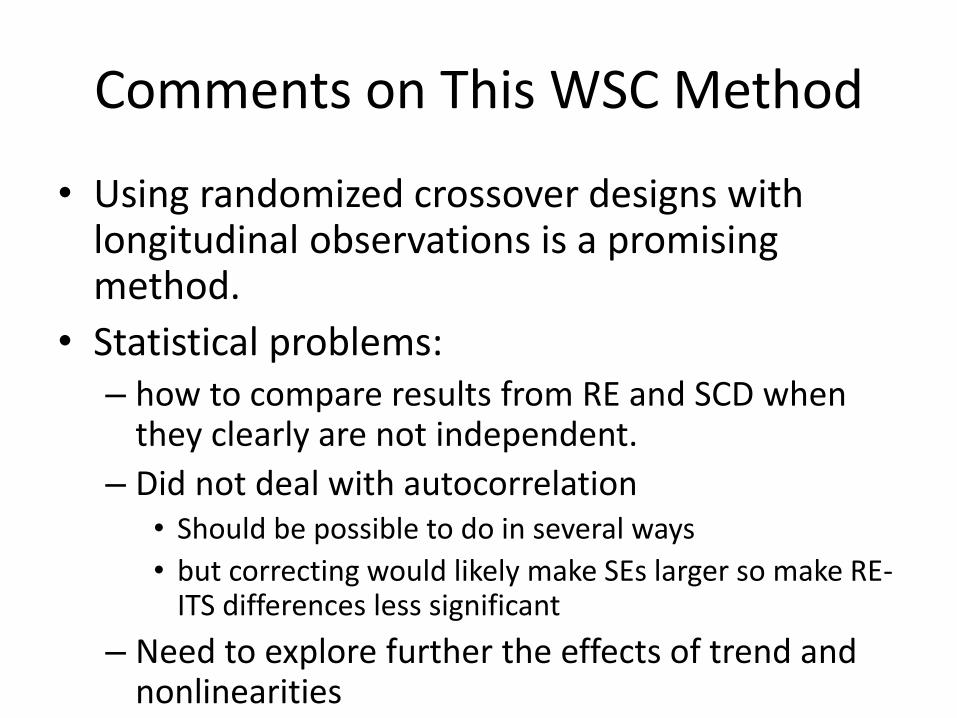
Comments on This WSC Method

• Using randomized crossover designs with longitudinal observations is a promising method.

• Statistical problems: – how to compare results from RE and SCD when

they clearly are not independent.

– Did not deal with autocorrelation • Should be possible to do in several ways

• but correcting would likely make SEs larger so make RE-ITS differences less significant

– Need to explore further the effects of trend and nonlinearities

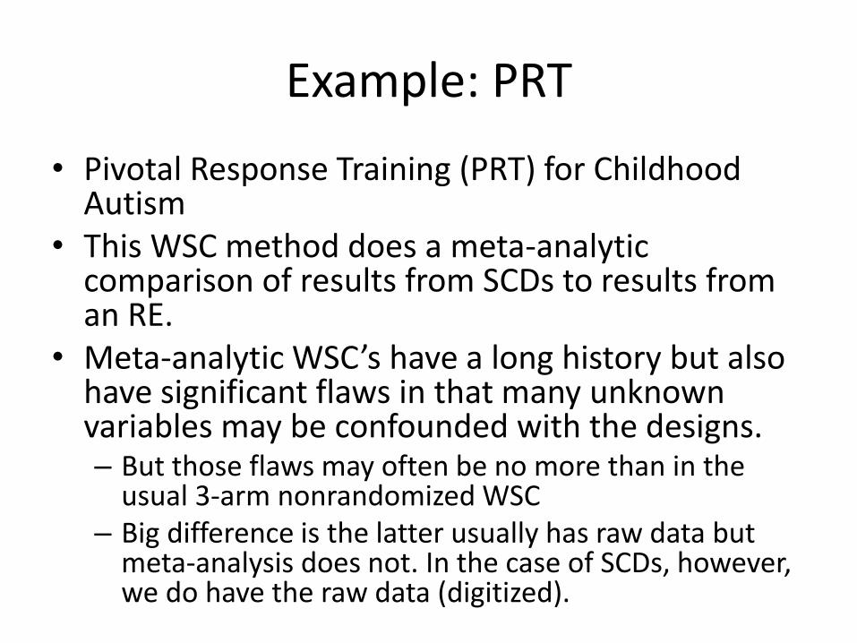
Example: PRT

• Pivotal Response Training (PRT) for Childhood Autism

• This WSC method does a meta-analytic comparison of results from SCDs to results from an RE.

• Meta-analytic WSC’s have a long history but also have significant flaws in that many unknown variables may be confounded with the designs. – But those flaws may often be no more than in the

usual 3-arm nonrandomized WSC – Big difference is the latter usually has raw data but

meta-analysis does not. In the case of SCDs, however, we do have the raw data (digitized).

The PRT Data Set

• Pivotal Response Training (PRT) for Childhood Autism

• 18 studies containing 91 cases.

• We used only the 14 studies with at least 3 cases (66 cases total).

• If there were only one outcome measure per study, this would result in 14 effect sizes.

• But each study measures multiple outcomes on cases, so the total number of effect sizes is 54

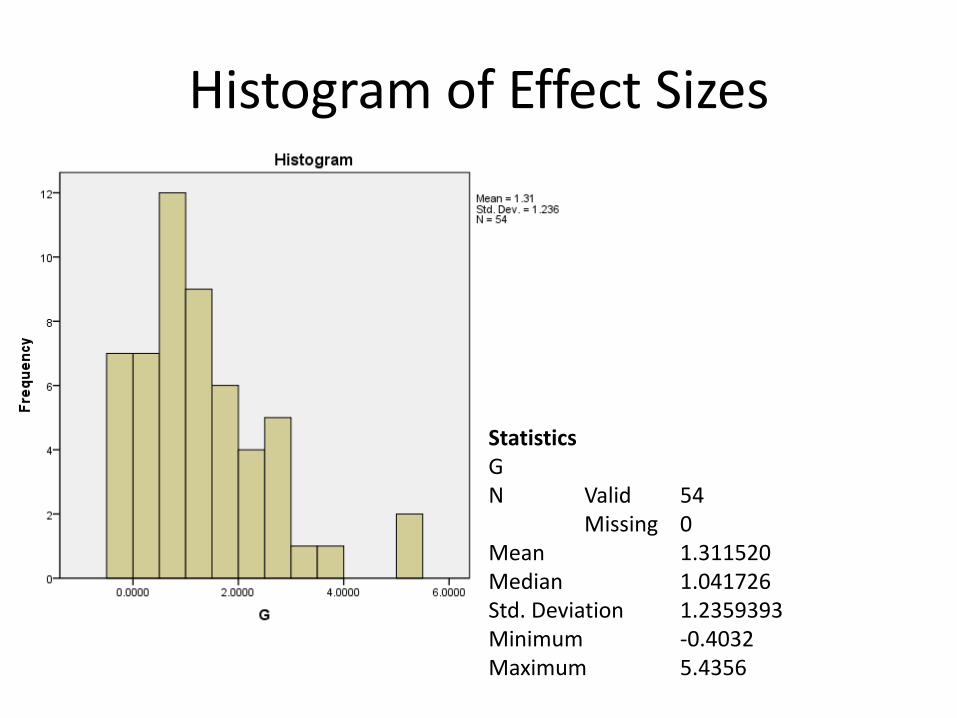
Histogram of Effect Sizes

Statistics G N Valid 54 Missing 0 Mean 1.311520 Median 1.041726 Std. Deviation 1.2359393 Minimum -0.4032 Maximum 5.4356

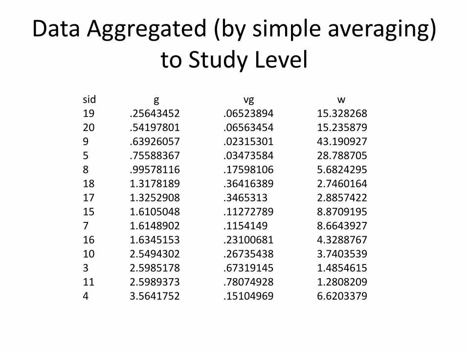
Data Aggregated (by simple averaging) to Study Level

sid g vg w 19 .25643452 .06523894 15.328268 20 .54197801 .06563454 15.235879 9 .63926057 .02315301 43.190927 5 .75588367 .03473584 28.788705 8 .99578116 .17598106 5.6824295 18 1.3178189 .36416389 2.7460164 17 1.3252908 .3465313 2.8857422 15 1.6105048 .11272789 8.8709195 7 1.6148902 .1154149 8.6643927 16 1.6345153 .23100681 4.3288767 10 2.5494302 .26735438 3.7403539 3 2.5985178 .67319145 1.4854615 11 2.5989373 .78074928 1.2808209 4 3.5641752 .15104969 6.6203379

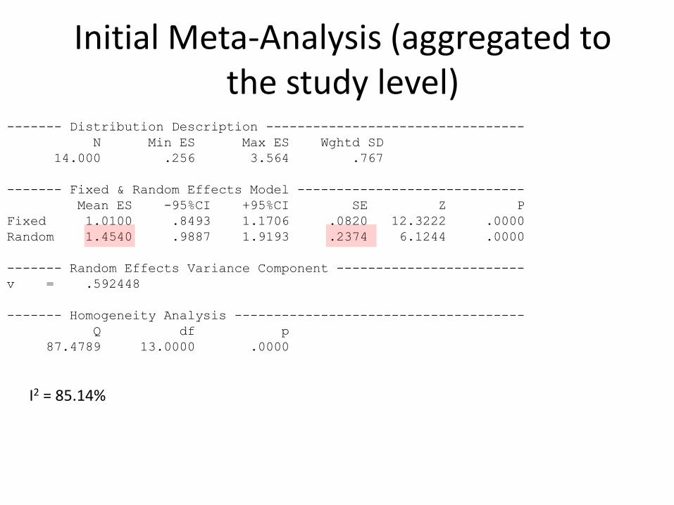
Initial Meta-Analysis (aggregated to the study level)

I2 = 85.14%

------- Distribution Description ---------------------------------

N Min ES Max ES Wghtd SD

14.000 .256 3.564 .767

------- Fixed & Random Effects Model -----------------------------

Mean ES -95%CI +95%CI SE Z P

Fixed 1.0100 .8493 1.1706 .0820 12.3222 .0000

Random 1.4540 .9887 1.9193 .2374 6.1244 .0000

------- Random Effects Variance Component ------------------------

v = .592448

------- Homogeneity Analysis -------------------------------------

Q df p

87.4789 13.0000 .0000

RE on PRT: Nefdt et al. (2010)

• From one RE (Nefdt et al., 2010), we selected the outcomes most similar to those used in the SCDs – G = .875, v(G) = .146 (se = .382).

• Recall that the meta-analysis of PRT showed – G = 1.454, V(G) = .056 (se = .2374)

• Are they the same? – Same direction, somewhat different magnitudes

– Again using 84% confidence interval overlap test: • .338 < .875 < 1.412 for RE

• 1.120 < 1.454 < 1.788 for SCDs

• Again, the confidence intervals overlap substantially, so no significant difference between RE and SCD

Comments on PRT Meta-Analytic Example

• This is just a very rough first stab

• Need to deal better with linearity issues in SCD analyses – We are currently expanding our d-statistic to cases

with nonlinearity

– In the meantime, can detrend prior to analysis

• Need also to code possible covariates confounded with the design for meta-regression.

Some Other Possible Examples

• Labor Economics (Dan Black)

– Many randomized experiments in labor economics use outcomes that are in archives with 20-30 data points

• Army Recruiting Experiment (Coady Wing)

– Incentive provided for enlisting into select specialties, but only in randomly selected recruiting districts.

– Could tap VA/SSA/etc records for outcomes

Issues in WSCs comparing ITS to RE

• Design Issues and Options

• Analytic Issues

• Logistical Issue

Design Issue: How to Make Random Assignment to RE vs ITS More Feasible in Four-Arm Study

• How to motivate people to take multiple measures so that attrition is not a problem in the time series? – Large amounts of money for each observation?

• E.g., 300 people times 12 observations times $100 per session = $360,000

• If 100 observations, total cost is $3,000,000, but how to space observations in a policy relevant way?

• Do pilot study to determine optimal payment per observation.

– Shorten overall time by using very frequent measurements per day (e.g., mood literature). • Could then reduce costs by paying per day or the like • But how policy relevant?

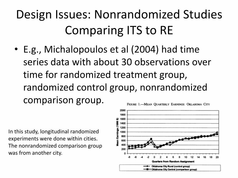
Design Issues: Nonrandomized Studies Comparing ITS to RE

• E.g., Michalopoulos et al (2004) had time series data with about 30 observations over time for randomized treatment group, randomized control group, nonrandomized comparison group.

In this study, longitudinal randomized experiments were done within cities. The nonrandomized comparison group was from another city.

More on Michalopolous • They did not analyze the ITS as a time series.

Instead just substituted the comparison group for the control group and analyzed like a randomized experiment. This is not how an ITS would be analyzed.

• In addition, this has the usual confounds between method and third variables.

• But this perhaps can and should be done more – Does someone want to reanalyze Michalopolous?

• Compare results from usual randomized estimate at one time point to – Analyzing the randomized control as ITS

Design Issues: Randomized Crossover Designs

• Key Issue: How many longitudinal randomized crossover designs exist with enough data points? – Medline search for “randomized crossover design” found

27986 hits. Surely some of these are longitudinal

– Medline Search for “longitudinal randomized crossover design” found 126 hits. But a quick look suggested few were what we need. So it will be a tedious search to find truly longitudinal randomized crossover designs

– I have a list of

– This is another good study for someone to do.

• Might need meta-analytic summary, so statistical issues will emerge about what effect size to use and how to deal with trend.

Design Issues: Meta-Analytic Approaches

• Feasible in areas where both ITS and REs are commonly used – A key issue would be to find areas with both

(medicine and N-of-1 trials? SCDs in ed and psy)

– My lab is currently working on this

• In many respects just aggregations of three and four arm studies with all the flaws and strengths therein. – But meta-regression could help clarify some

confounds of methods with third variables.

Analytic Issues

• Because so many real examples are short ITS, usual ARIMA modeling etc is not practical.

• Key analytic issues:

– What is the metric for the comparison of ITS and RE?

– Dealing with trend

– Dealing with autocorrelation

Analytic Issues: When the Metric is the Same

• To compare RE to ITS, the same effect estimate has to be measured in the same metric

• Not a problem – In longitudinal randomized crossover designs – In three arm studies in which participants are randomized to all

methods and treated identically and simultaneously (e.g., Shadish et al., 2008, 2011)

– In three-arm studies like Michalopolous that are all part of one large study

– Or over multiple studies if they just happened to use the same outcome variable.

• In all cases, ensure the effect estimate is the same (ATE, ToT, etc.).

• But meta-analyzing all this can require finding a common metric if it causes metrics to differ across studies.

Analytic Issues: Metric Is Different

• Special Case: When all outcomes are dichotomous but may measure different constructs

– Can use HLM (etc) with code for outcome type (Haddock Rindskopf Shadish 1998)

• Otherwise, need common effect size estimate like d, r, odds ratio, rate difference, etc.:

Analytic Issue: Metric is Different

• d-statistic for ABk SCDs (Hedges, Pustejovsky and Shadish in press RSM) – SPSS macro in progress; R-script available but needs individual

adaptation to each study – Assumes no trend, normally distributed outcome – Takes autocorrelation and between-within case variability into

account; requires minimum 3 cases.

• d-statistic for multiple baseline designs SCDs nearing completion (HPS also)

• Grant proposal pending to extend work to – Various kind of trend – Various kinds of outcome (e.g., counts distributed as Poisson or

binomial)

• There are other effect sizes, but none are well-justified statistically, or comparable to between groups effect sizes.

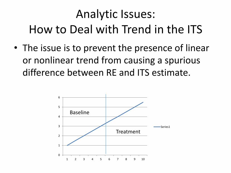
Analytic Issues: How to Deal with Trend in the ITS

• The issue is to prevent the presence of linear or nonlinear trend from causing a spurious difference between RE and ITS estimate.

0

1

2

3

4

5

6

1 2 3 4 5 6 7 8 9 10

Series1

Treatment

Baseline

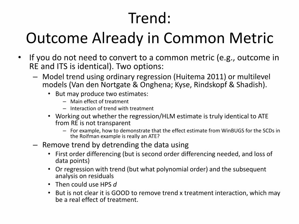
Trend: Outcome Already in Common Metric

• If you do not need to convert to a common metric (e.g., outcome in RE and ITS is identical). Two options: – Model trend using ordinary regression (Huitema 2011) or multilevel

models (Van den Nortgate & Onghena; Kyse, Rindskopf & Shadish). • But may produce two estimates:

– Main effect of treatment – Interaction of trend with treatment

• Working out whether the regression/HLM estimate is truly identical to ATE from RE is not transparent

– For example, how to demonstrate that the effect estimate from WinBUGS for the SCDs in the Roifman example is really an ATE?

– Remove trend by detrending the data using • First order differencing (but is second order differencing needed, and loss of

data points) • Or regression with trend (but what polynomial order) and the subsequent

analysis on residuals • Then could use HPS d • But is not clear it is GOOD to remove trend x treatment interaction, which may

be a real effect of treatment.

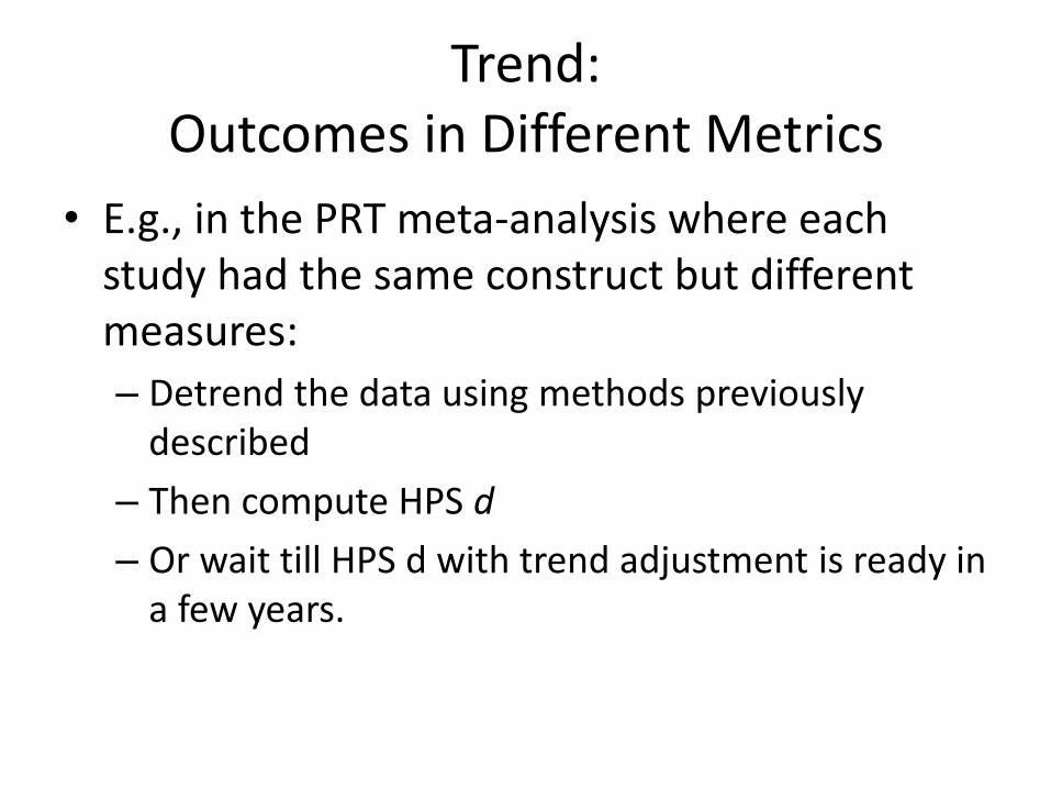
Trend: Outcomes in Different Metrics

• E.g., in the PRT meta-analysis where each study had the same construct but different measures:

– Detrend the data using methods previously described

– Then compute HPS d

– Or wait till HPS d with trend adjustment is ready in a few years.

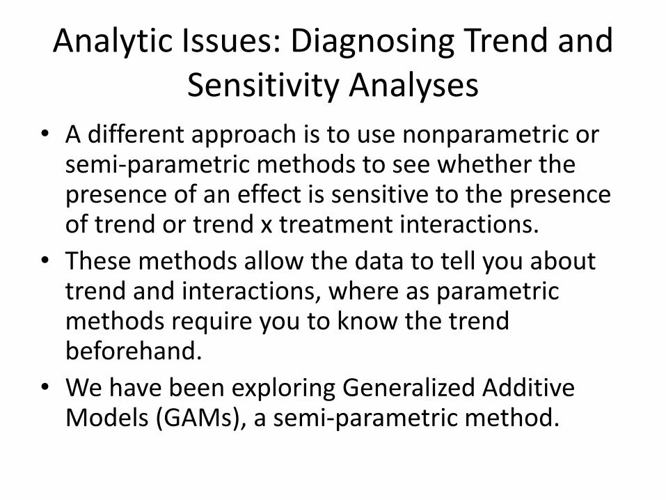
Analytic Issues: Diagnosing Trend and Sensitivity Analyses

• A different approach is to use nonparametric or semi-parametric methods to see whether the presence of an effect is sensitive to the presence of trend or trend x treatment interactions.

• These methods allow the data to tell you about trend and interactions, where as parametric methods require you to know the trend beforehand.

• We have been exploring Generalized Additive Models (GAMs), a semi-parametric method.

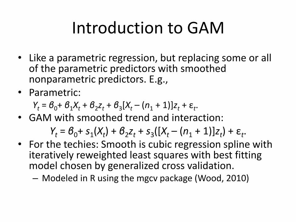
Introduction to GAM

• Like a parametric regression, but replacing some or all of the parametric predictors with smoothed nonparametric predictors. E.g.,

• Parametric: Yt = β0+ β1Xt + β2zt + β3[Xt – (n1 + 1)]zt + εt.

• GAM with smoothed trend and interaction: Yt = β0+ s1(Xt) + β2zt + s3([Xt – (n1 + 1)]zt) + εt.

• For the techies: Smooth is cubic regression spline with iteratively reweighted least squares with best fitting model chosen by generalized cross validation. – Modeled in R using the mgcv package (Wood, 2010)

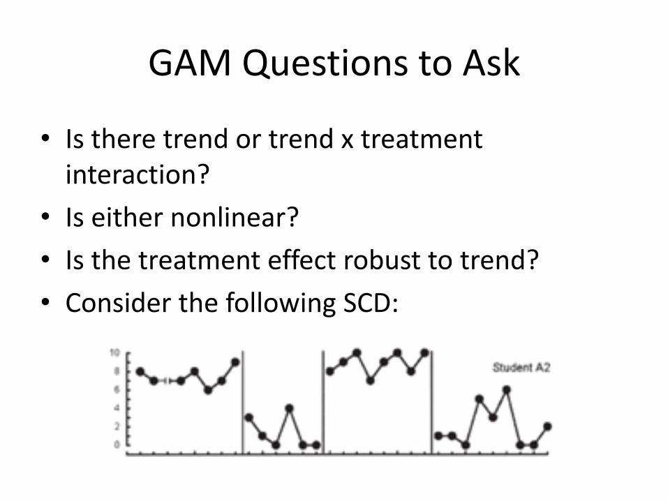
GAM Questions to Ask

• Is there trend or trend x treatment interaction?

• Is either nonlinear?

• Is the treatment effect robust to trend?

• Consider the following SCD:

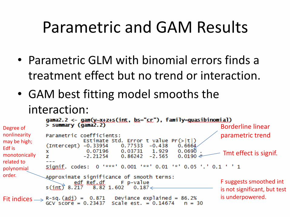
Parametric and GAM Results

• Parametric GLM with binomial errors finds a treatment effect but no trend or interaction.

• GAM best fitting model smooths the interaction:

Fit indices

Borderline linear parametric trend

Tmt effect is signif.

Degree of nonlinearity may be high; Edf is monotonically related to polynomial order.

F suggests smoothed int is not significant, but test is underpowered.

GAM Conclusions • About our three questions:

– A trend by treatment might be present

– If so, it may be highly nonlinear

– But the treatment effect is robust to trend compared to the usual GLM.

• About GAM based on our experience so far: – Works well with > 20 data points, less sure < 20

– Good as sensitivity analysis about trend, too early to say if good as primary analysis of ITS effects.

– Open power questions • Model comparison tests seem well powered (too well?)

• F test for smooth is said to be underpowered.

– Does GAM overfit the data?

Conclusions about Trend

• Probably the most difficult problem for WSCs of RE and ITS

• Lots of methods available and in development but no “best practice” yet

– So multiple sensitivity analyses warranted

• Decision about trend depends in part on decision/context regarding metric

– If all outcomes are the same, more flexibility.

– If outcomes vary, detrend, use d, use GAM for sensitivity analyses?

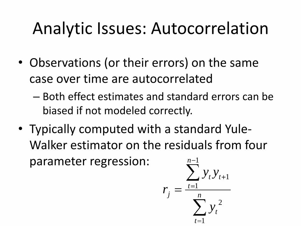
Analytic Issues: Autocorrelation

• Observations (or their errors) on the same case over time are autocorrelated

– Both effect estimates and standard errors can be biased if not modeled correctly.

• Typically computed with a standard Yule-Walker estimator on the residuals from four parameter regression:

1

1

1

2

1

n

t t

tj n

t

t

y y

r

y

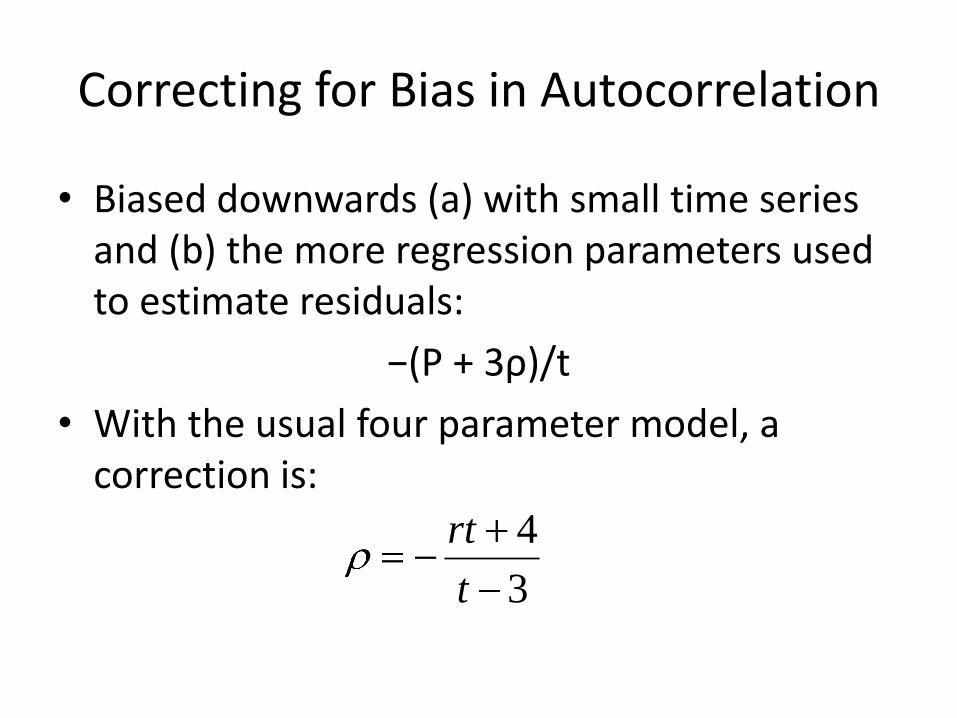
Correcting for Bias in Autocorrelation

• Biased downwards (a) with small time series and (b) the more regression parameters used to estimate residuals:

−(P + 3ρ)/t

• With the usual four parameter model, a correction is:

4

3

rt

t

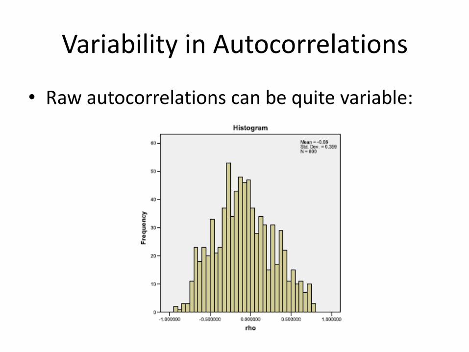
Variability in Autocorrelations

• Raw autocorrelations can be quite variable:

Autocorrelation and Sampling Error

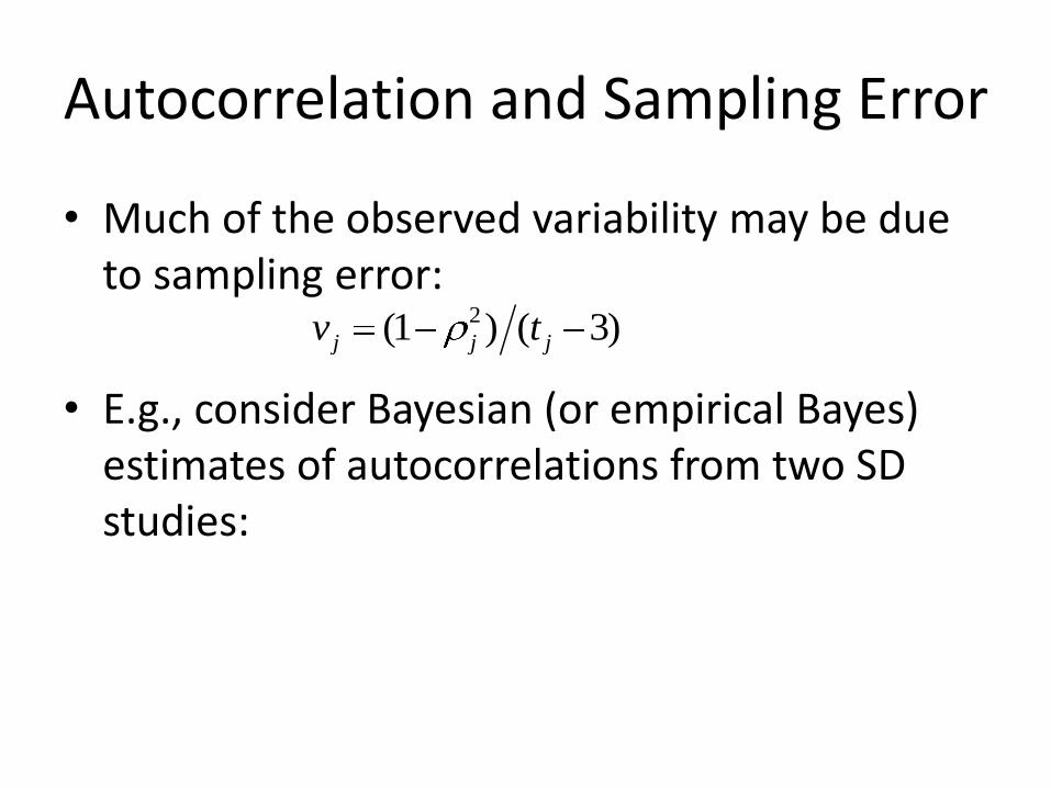
• Much of the observed variability may be due to sampling error:

• E.g., consider Bayesian (or empirical Bayes) estimates of autocorrelations from two SD studies:

2(1 ) ( 3)j j jv t

Trace Plot for Schutte Data

0.005 0.013 0.030 0.065 0.140 0.303 0.668 1.558 4.157

0.0

0.0

50

.10

0.1

50

.20

0.2

50

.30

0.3

5

Tau

Pos

teri

or

Pro

bab

ility

of

Ta

u

A A A A A A A A AB B B B

B

B

BB B

C C CC

C

C

C

C C

D D D D DD

DD D

E E E EE

E

EE E

F F F F FF

F F F

G G G G

G

G

GG G

H H H HH

H

HH H

I I I II

I

I

I I

J J J J J JJ J J

K K K K KK

KK K

L L L L L L L L LM M M M

M

M

M

MM

N N N N NN

N N N

Estimates Conditional on Tau

A=(Intercept) B=1 C=2 D=3 E=4 F=5 G=6 H=7 I=8 J=9 K=10 L=11 M=12 N=13

-0.8

-0.6

-0.4

-0.2

0.0

0.2

0.4

Con

ditio

na

l M

ea

n

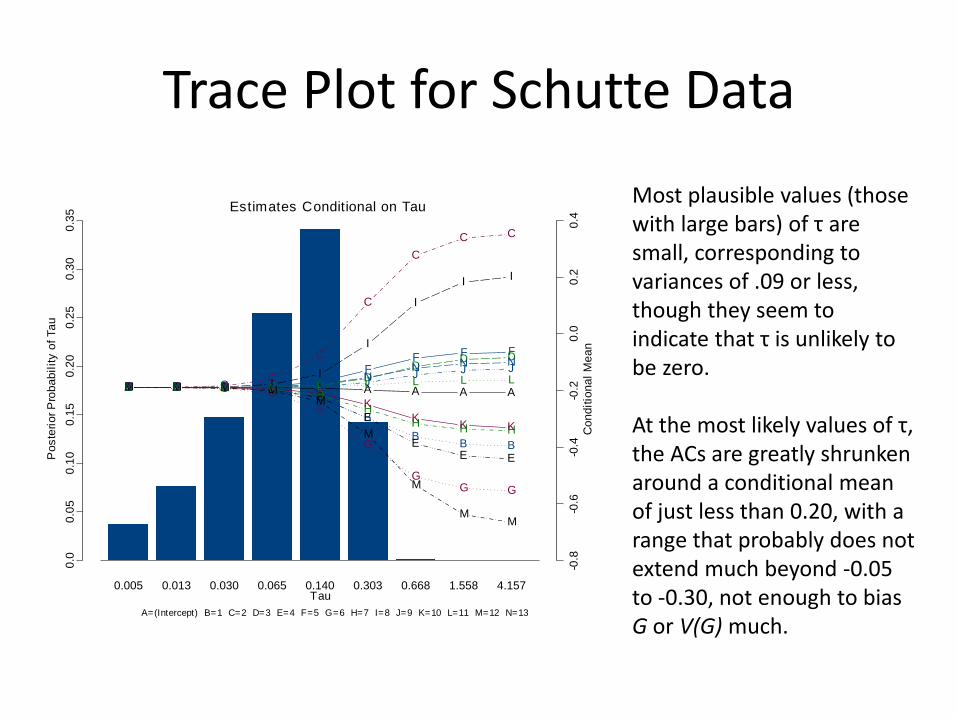
Most plausible values (those with large bars) of τ are small, corresponding to variances of .09 or less, though they seem to indicate that τ is unlikely to be zero. At the most likely values of τ, the ACs are greatly shrunken around a conditional mean of just less than 0.20, with a range that probably does not extend much beyond -0.05 to -0.30, not enough to bias G or V(G) much.

Trace Plot for Dyer Data

0.025 0.048 0.085 0.143 0.239 0.399 0.676 1.189 2.288

0.0

0.0

50

.10

0.1

50

.20

0.2

50

.30

0.3

50

.40

Tau

Pos

teri

or

Pro

bab

ility

of

Ta

u

A A A A A A A A AB BB

B

BB B B B

CC

C

C

CC C C C

D

D

D

D

D

D

DD D

EE

E

E

EE

E E E

Estimates Conditional on Tau

A=(Intercept) B=1 C=2 D=3 E=4

-0.3

-0.2

-0.1

0.0

0.1

0.2

0.3

0.4

Con

ditio

na

l M

ea

n

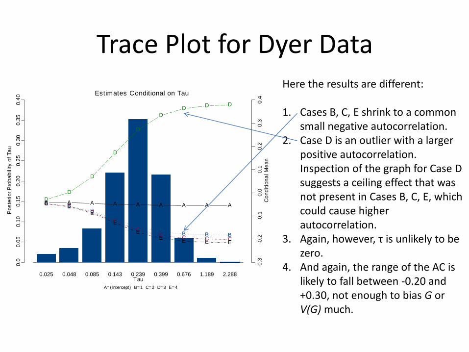
Here the results are different: 1. Cases B, C, E shrink to a common

small negative autocorrelation. 2. Case D is an outlier with a larger

positive autocorrelation. Inspection of the graph for Case D suggests a ceiling effect that was not present in Cases B, C, E, which could cause higher autocorrelation.

3. Again, however, τ is unlikely to be zero.

4. And again, the range of the AC is likely to fall between -0.20 and +0.30, not enough to bias G or V(G) much.

Implications of Bayesian Results

• Doing Bayesian analyses of ITS/SCDs may be a very useful approach

• We need more research to understand whether assuming a common underlying (Bayesian or EB) autocorrelation is justified for, say, cases within studies. – Schutte data says yes

– Dyer data says no (but moderator analyses?)

• If we can make that assumption, much of the variability goes away and the remaining autocorrelation may be small enough to ignore

Dealing with Autocorrelations

• Lots of methods, but don’t ignore entirely

• In GLM/HLM/GAM: – Incorrect specification of trend in such models can

lead to spurious autocorrelations, so modeling trend is important to results

– Tentative work (GAMs) suggests properly modeling trend may reduce ACs to levels that are unimportant for bias.

• For d, our SPSS macro estimates AC and adjusts d appropriately.

Logistical Issue • How to get the data for the time series.

– Sometimes it is available in an archive etc. – Sometimes it has to be digitized from graphs

• The latter can be done with high validity and reliability: – Shadish, W.R., Brasil, I.C.C., Illingworth, D.A., White, K.,

Galindo, R., Nagler, E.D. & Rindskopf, D.M. (2009). Using UnGraph® to Extract Data from Image Files: Verification of Reliability and Validity. Behavior Research Methods, 41, 177-183.

– There is freeware also.

• But digitizing can be time consuming and tedious for large numbers of studies – E.g., a very good graduate student digitizing 800 SCDs from

100 studies took 8 months (including coding; Shadish & Sullivan 2011).

Questions to Ask • The one area where we still need studies on

the main effect question of “can ITS = RE?”

• Design variations to also examine:

– Does it help to add a nonequivalent control?

– Does it help to add a nonequivalent DV?

– What about variations in ITS design?

• Ordinary ITS with one intervention at one time

• Multiple baseline designs with staggered implementation of intervention over time – Over cases

– Over measures within one case

Conclusion

• WSCs of ITS and RE badly needed if ITS is going to regain the credibility it once had (assuming it does, in fact, give a good answer).

• Challenging to design and analyze, but much progress has been made already, especially in SCDs and N-of-1 Trials.

• Questions?

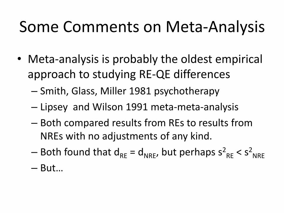
Some Comments on Meta-Analysis

• Meta-analysis is probably the oldest empirical approach to studying RE-QE differences

– Smith, Glass, Miller 1981 psychotherapy

– Lipsey and Wilson 1991 meta-meta-analysis

– Both compared results from REs to results from NREs with no adjustments of any kind.

– Both found that dRE = dNRE, but perhaps s2RE < s2

NRE

– But…

How Much Credibility Should We Give To Such Studies?

• The RE-NRE question was always secondary to substantive interests (does psychotherapy work; do behavioral and educational interventions work?) – So no careful attention to definitions of RE-NRE

• Just used original researchers word for it

– No attention to covariates confounded with RE-NRE.

• Glaser (my student) carefully recoded a large random sample of Lipsey and Wilson using clear definitions etc, and found LW’s finding did not replicate.

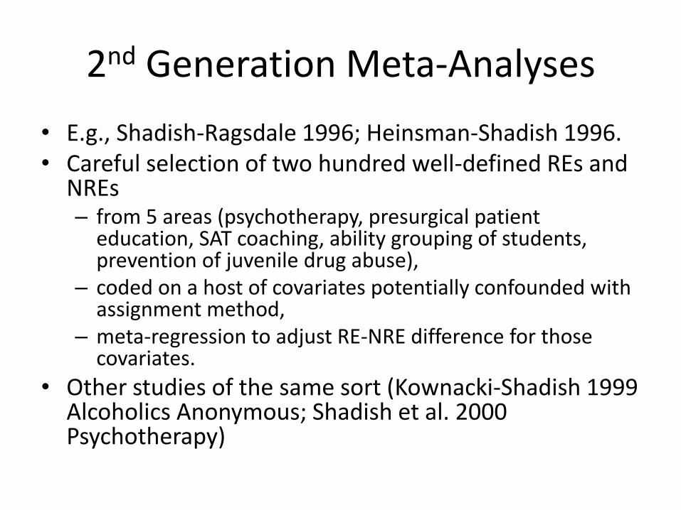
2nd Generation Meta-Analyses

• E.g., Shadish-Ragsdale 1996; Heinsman-Shadish 1996. • Careful selection of two hundred well-defined REs and

NREs – from 5 areas (psychotherapy, presurgical patient

education, SAT coaching, ability grouping of students, prevention of juvenile drug abuse),

– coded on a host of covariates potentially confounded with assignment method,

– meta-regression to adjust RE-NRE difference for those covariates.

• Other studies of the same sort (Kownacki-Shadish 1999 Alcoholics Anonymous; Shadish et al. 2000 Psychotherapy)

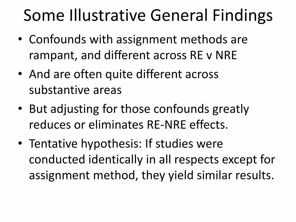
Some Illustrative General Findings • Confounds with assignment methods are

rampant, and different across RE v NRE

• And are often quite different across substantive areas

• But adjusting for those confounds greatly reduces or eliminates RE-NRE effects.

• Tentative hypothesis: If studies were conducted identically in all respects except for assignment method, they yield similar results.

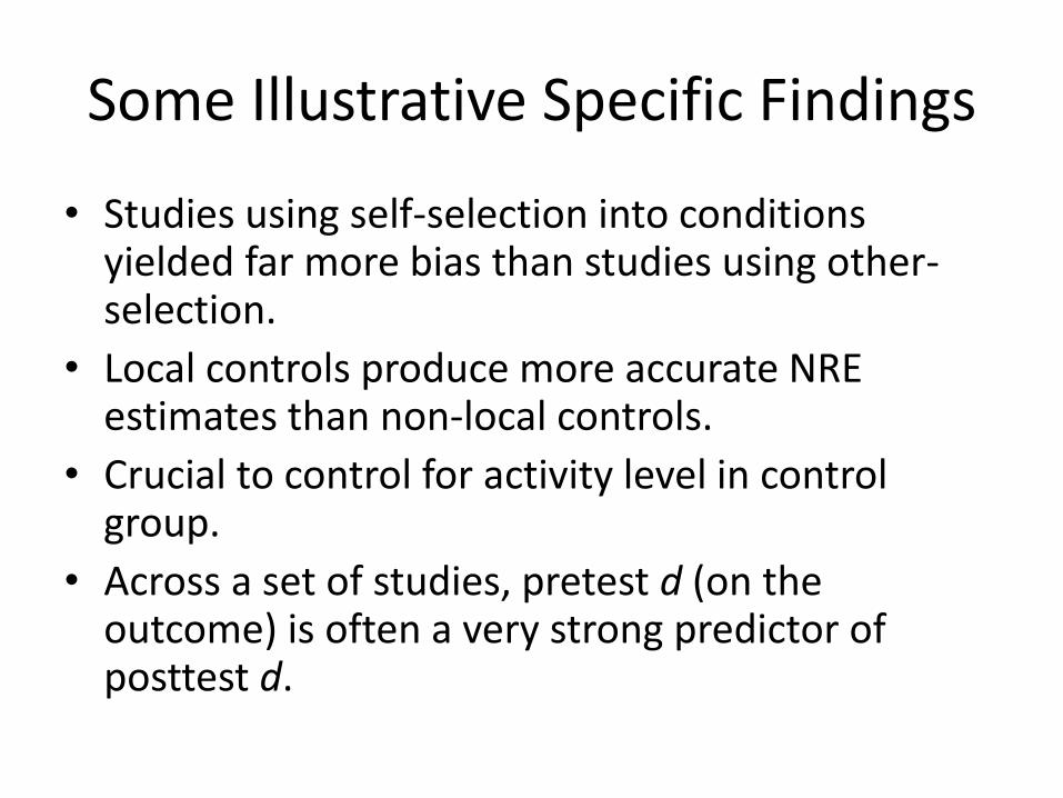
Some Illustrative Specific Findings

• Studies using self-selection into conditions yielded far more bias than studies using other-selection.

• Local controls produce more accurate NRE estimates than non-local controls.

• Crucial to control for activity level in control group.

• Across a set of studies, pretest d (on the outcome) is often a very strong predictor of posttest d.

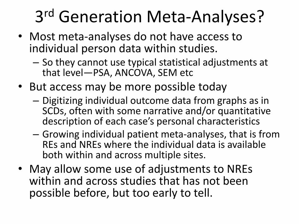
3rd Generation Meta-Analyses? • Most meta-analyses do not have access to

individual person data within studies. – So they cannot use typical statistical adjustments at

that level—PSA, ANCOVA, SEM etc

• But access may be more possible today – Digitizing individual outcome data from graphs as in

SCDs, often with some narrative and/or quantitative description of each case’s personal characteristics

– Growing individual patient meta-analyses, that is from REs and NREs where the individual data is available both within and across multiple sites.

• May allow some use of adjustments to NREs within and across studies that has not been possible before, but too early to tell.

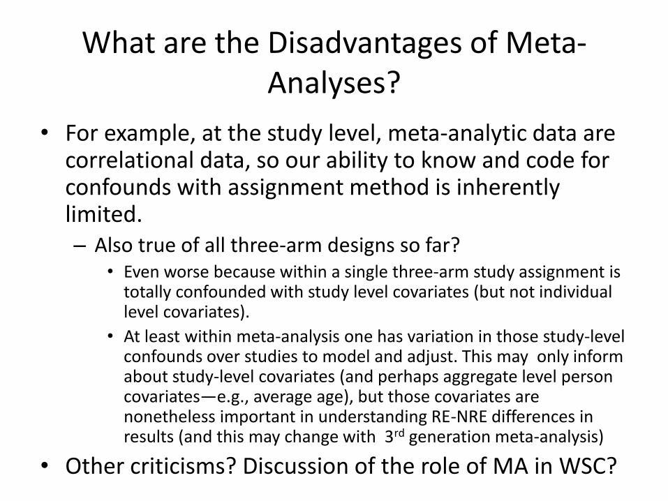
What are the Disadvantages of Meta-Analyses?

• For example, at the study level, meta-analytic data are correlational data, so our ability to know and code for confounds with assignment method is inherently limited. – Also true of all three-arm designs so far?

• Even worse because within a single three-arm study assignment is totally confounded with study level covariates (but not individual level covariates).

• At least within meta-analysis one has variation in those study-level confounds over studies to model and adjust. This may only inform about study-level covariates (and perhaps aggregate level person covariates—e.g., average age), but those covariates are nonetheless important in understanding RE-NRE differences in results (and this may change with 3rd generation meta-analysis)

• Other criticisms? Discussion of the role of MA in WSC?