INTERACTIVE TOOL FOR MOBILE

ROBOT MOTION PLANNING

J.L. Guzman∗ a, M. Berenguel a, F. Rodrıguez a, S. Dormido b

aDep. Lenguajes y Computacion, Universidad de Almerıa, Ctra. Sacramento s/n04120 Almerıa, Spain. Tlf: + 34 950015849. Fax: + 34 950015129.

E-mail:joguzman@ual.esbDep. Informatica y Automatica, ETSI Informatica, UNED, C. Juan del Rosal, 16

28040 Madrid, Spain.

Abstract

Mobile robotics is a subject included in several engineering curricula at present. Thecontinuous increase in computer processing power allows the use of interactive toolsto merge the synthesis and analysis phases of classical engineering iterative designtechniques into one, being possible to apply these advantages to the robotics field.An interactive tool is presented in this work aimed at facilitating the understandingof several well-known algorithms and techniques involved in solving mobile robotmotion problems, from those modelling the mechanics of mobility to those used innavigation. The paper also discuses how the tool can be used in an introductorycourse of mobile robotics.

Key words: mobile robotics, interactivity, simulation, kinematics, robot motion

1 Introduction

This paper presents an interactive tool for understanding basic concepts in-volved in mobile robotics, and also discusses how it can be used in an in-troductory course. Interactive tools are becoming key elements in differentengineering courses and mobile robotics is an educational field where the ad-vantages of this learning paradigm can be better exploited. The theory canbe learned through textbooks, inspiring lectures, and active study. The abilityto solve practical problems relies on good skill in using theory and in break-ing down large problems into manageable subproblems. One of the importanttasks for teachers in engineering is to transmit to the students not only theformal and logic structure of the discipline, but also, and certainly with muchmore emphasis, the strategic and intuitive aspects of the subject [15]. These

Preprint submitted to Robotics and Autonomous Systems 1 March 2007

Manuscript

last aspects are probably much more difficult to make explicit and assimilatefor students, precisely because they lie very often in the less conscious sub-strata of the expert’s activity. Interactive tools are considered a great stimulusfor developing the student’s intuition and they attempt to demystify abstractmathematical concepts through visualization for specifically chosen examples[14]. Although the term Interactivity can be defined in several ways [14], froma teaching point of view an Interactive Tool can be defined as a collection ofgraphical windows whose components are active, dynamic, and/or clickable;and that is intended to explain just a few concepts. The use of interactive andinstructional graphic tools would reinforce active participation of students.For educators, this kind of tools can provide a very useful way to test mainideas and to realize how difficult explaining a particular concept to studentsis [14,31].

Mobile robotics is a relatively new research area that deals with the controlof autonomous and semiatonomus vehicles. It is the domain where literallythe ”rubber meets the road” for many algorithms in path planning, knowl-edge representation, sensing and reasoning. An autonomous mobile robot is amachine able to extract information from its environment and use knowledgeabout its world to move safely in a meaningful and purposive manner, it canoperate on its own without a human directly controlling it [8]. The primarytask of a mobile robot is environmental navigation as basis for more usefultasks.

In other words, mobile robotics deals with the problem of moving a mobilerobot in any environment following a free collision path. It involves manytasks related to algorithms for path planning and tracking, knowledge repre-sentation, sensing, and reasoning. For this reason, mobile robotics combinesmany disciplines, including electrical engineering, automatic control, computerscience, mechanical engineering, artificial intelligent and others [2]. Mobilerobotics can be understood as a navigation problem, described as the actionof directing a mobile robot to traverse a specific environment. The main aim inany navigation scheme is to reach a destination without moving away from thegoal or crashing with objects [25], [2]. Navigation is divided into three tasks:mapping, planning and tracking [17], [25]. If the map of the environment isconsidered as an input to the system (the mapping problem has been solved),and under a typical 2D navigation assumption [17], [25], [2] the navigationprocess involves two kinds of problems:

• Path planning. It is a geometric problem related with the robot dimensionsand the obstacles located in the navigation space. Its solution provides asequence of positions that joins the initial and goal points defining the freetrajectory (without obstacles) to be followed by the robot.

• Path tracking. It is a control problem related with the constraints on therobot movements, actuators, and the time elapsed in the navigation. Its so-

2

lution provides, all the time, the set point to each actuator aimed at reachingor following (sometimes in a prescribed time) the trajectory obtained whensolving the geometric problem.

In this work, a typical basic course of mobile robot motion planning has beenfollowed, as that described in [2] which is used in the Massachusetts Instituteof Technology (MIT) and other prestigious universities listed in http://www-cvr.ai.uiuc.edu/∼seth/RMPbook/. The aim of the interactive tool presentedin this paper is to help studying the classical notion paradigms, basicallyfocused on[2]:

• Roadmap algorithms, like Visibility graph and Voronoi Diagram.• Potential algorithms like Potential Functions and Wave front.• Bug algorithms.• Cellular decomposition.

Evidently, there exist other algorithms within the previous paradigms notincluded in the tool, such as the Probabilistic Methods (Probabilistic RoadmapPlanning, Expansive-Spaces Tree Planning or Probabilistic Roadmap of Tree,etc.) [2], which are susceptible to be included in the tool in the future.

The solution of the path planning task depends on the knowledge the robothas of the navigation space, so the previous algorithms can be grouped consid-ering this idea. Basically, global algorithms (such as Visibility Graph, VoronoiDiagram, Cell decomposition, and Wave front) will be used if the dimensionsand locations of all the obstacles are well-known (deliberative navigation). Ifthis information is unknown, the use of local algorithms (such as Bug and Po-tential function algorithms) is required (reactive navigation). With both globaland local algorithms it is necessary to know or estimate the robot position ateach time. In real applications different techniques and/or sensors are used toobtain the actual robot position (odometry, inertial methods, GPS, etc.). Theintegration of the robot kinematics or dynamics provides an approximationto the real position that can be used for simulation purposes, as done in thisapplication.

Therefore, mobile robotics involves many disciplines and the navigation prob-lem requires several steps that must be well studied and understood by engi-neering students. Based on the authors’ experience, teaching and learning ofthe involved concepts could be addressed using the new interactive method-ologies developed during the last years and having a great impact in the fieldof Automatic Control [14,18,35,4,11,7]. As commented in [7], the continuousincrease in computer processing power allows the use of interactive tools tomerge the synthesis and analysis phases of classical engineering iterative designtechniques into one, in such a way that the modification of any configuration,parameter, or element in the system produces an immediate effect in the rest

3

and thus the design procedure becomes really dynamic, allowing to identifymuch more easily the compromises that can be achieved. So, the main contri-bution of this paper is to present an interactive tool that helps teaching andlearning main concepts and techniques involved in mobile robotics by simula-tion over a 2D environment defined by the Cartesian coordinates (x , y). Thistool is being used in an introductory course of mobile robotics for ComputerScience engineering students.

2 Related work

The vertiginous advances that undergone the new teaching technologies havehad a great impact in the scope of robotics, mainly in the field of robot ma-nipulators. During the last years, multiple tools, virtual, and remote labs havebeen developed to allow the students work and learn at home or through theWWW from any part of the world without temporal constraints [5,3,33,32]and providing interactive learning [19]. Several teaching tools have also beenpublished in the field of mobile robotics (e.g. [10,1,4]), but with less impactthan those developed in the scope of robot manipulators.

In [9] an interactive autonomous robot motion planning system developed inJava is described. This interactive system enables users to set up the workingenvironment by creating obstacles and a robot of different shapes, specifyingstarting and goal positions and setting other path or environment parametersfrom a user-friendly interface. The main disadvantage of this tool is that onlydeliberative navigation is considered where the Minkowski sum and VisibilityGraph are the unique algorithms implemented. Furthermore, robot kinematicsare not used. On the other hand, an interactive system based on VirtualReality where the aim consists on reconstructing the real environment basedon the real sensor is presented in [27]. A simulation option is also includedwhere the robot is based on tricycle kinematics, the path planning is definedby the user where the operator enters several possible points to track, and theminimum path is obtained using Dijkstra’s algorithm [6].

Another tools are AMORsim [28], Khepera simulator [24], Stage [34], SIM-ROBOT [16], and HEMERO [23] which are mainly focused on particularkinematic study avoiding path planing problems. For instance, HEMERO isa toolbox for the study of manipulator and mobile robots. The tool combinesMatlab and Simulink for the representation the kinematic and dynamic mod-elling of the robots. The numerical results are illustrated by means of staticsimple graphics generated with Matlab without interactive behavior. The toolpresented in this paper has been oriented to cover the main features of theprevious tools in such a way that the different aspects considered in a basiccourse of mobile robotics are included. Its development was motivated twofold.

4

It can help the lecturer to show how mobile robots behave depending of theselected kinematics, path planning algorithms, and robot control algorithms.In addition, this tool can help the students to put into practice and under-stand themselves the learned concepts, and to analyze how algorithms behaveprevious to use them in real robots.

The tool presented in this work facilitates the understanding of the algorithmsused in solving mobile robotics problems. In the first version [13] the tool hadthe possibility of working with known environments and robots with differen-tial mechanism, where the navigation from the initial to the goal point wasperformed using a visibility graph algorithm for path planning and the purepursuit method for path tracking (similar to the tool presented in [10]). Theobjective of the current version of the tool is to extend its capabilities in someaspects. In the case of navigation algorithms, both global algorithms (usingglobal or vertex maps - Visibility graphs, free-space maps - Voronoi diagrams,composite-space maps - Quadtrees, propagation-space maps - WaveFront) andlocal algorithms (potential, BUG and VISBUG) have been considered.

Three different robot kinematics have also been included: differential mecha-nism, tricycle/Ackermann, and synchronous. Many different parameters canbe selected and/or modified using the tool user interface, such as those asso-ciated to the navigation algorithm, the initial and goal positions of the mobilerobot, the robot kinematics and associated dimensions, the number, morphol-ogy and position of different objects in the environment, etc. The user caninteractively visualize the effect that these modifications have on the robottrajectory to navigate from the initial to the goal position (the results canbe shown in one run or using a step by step procedure). The selection ofthe features included in the tool has been based on the typical contents ofintroductory courses of mobile robotics.

3 Description of the tool

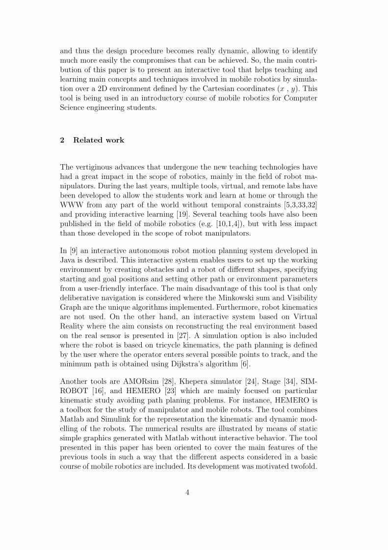
This section describes the main features of the tool, programmed with SysQuake,a Matlab-like [22] environment which has strong support for interactive graph-ics [29]. The interactive tool is free and available for Windows, Mac, and Linuxoperating systems [12]. Notice that the main feature of the tool - Interactiv-ity - is difficult to be highlighted in a written text. When developing a toolof this kind, the programming of the algorithms is a time consuming aspect,but one of the most important things that the teacher has to have in mind isthe organization of the main windows and menus of the tool to facilitate thestudent the understanding of the theoretical aspects [14]. The main windowof the tool is divided into several sections represented in Fig. 1 (basic screenof the tool) which are described in what follows:

5

Fig. 1. Main window of the tool showing an example.

• Environment : main window on the right side of the screen. It representsthe working space with a set of obstacles where the robot will evolve. It ispossible to change the morphology of the obstacles dragging with the mouseover their corners. The original objects are shown in black, their convexenvelopes are drawn using dotted lines, and the final object (the convexobstacle enlarged using the robot width) are presented in yellow. Both theorigin point (the robot) and the target point that the robot will try toreach can be modified over this graph. The results of the selected planningalgorithm are shown on the environment. The shortest path is drawn in red(for the global algorithms), and the path followed by the robot in greencolour.

• Operation mode: two operation modes are available in the tool and canbe modified using this option. The Configuration mode allows defining theenvironment, algorithms, and robot related options before running a simu-lation. The Algorithm mode is used to calculate the minimum-length path(if selected) and run the simulation.

• Algorithm selection and parameters: these two options allow choosing thedesired planning algorithm and associated parameters (see Table 1). Theparameters of the pure pursuit algorithm implemented for path trackingpurposes can also be changed.

• Robot parameters and kinematics: the different initial robot parameters suchas size, speed, orientation, and wheel radius can be modified. On the otherhand, it is possible to select the robot morphology between differential mech-

6

anism, tricycle, and synchronous (see Table 1).• Obstacle insertion: it allows inserting a new obstacle into the environment,

this option being available on the left-bottom corner of the tool. First, themorphology of the obstacle is selected between several options: triangle,rectangle or free polygon. After this selection, the mouse pointer can beplaced on the environment location in which the obstacle will be inserted,and then a single click on the left mouse button will perform the action. Inthe case of the free polygon option, the number of sides must be selectedusing the slider Sides.

• Control signals : two graphics on the bottom right of the interface (Fig.1) show the evolution of the control signals of the selected kinematics (theangular velocities of the left and right wheels, ωi and ωd in Fig. 1 because thedifferential kinematic is chosen). Amplitude and/or rate input constraintscan be included by dragging in the tool the red vertical lines shown in thegraphs.

Fig. 2. Settings menu.

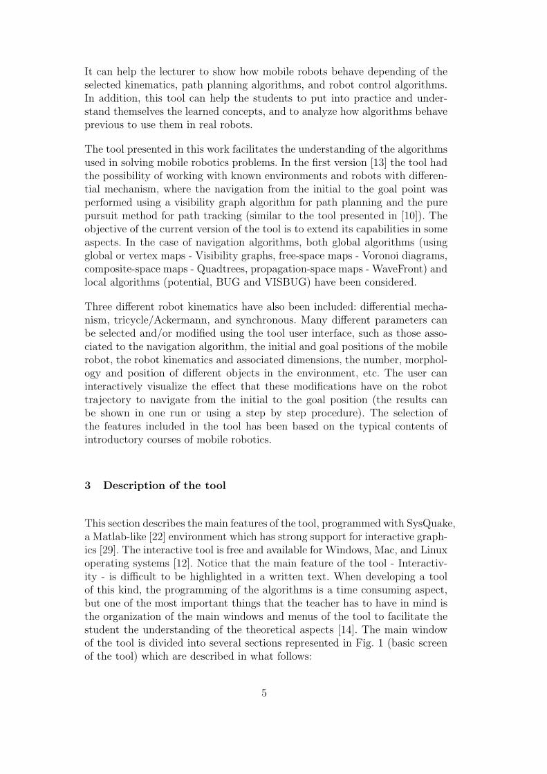
• Settings Menu: it is possible to start, pause, and stop the simulation andto show the results step by step. All the options available in the graphicalinterface can be also modified from this menu (see Fig. 2).

Fig. 3 describes the steps that have to be performed when using the tool.These steps have been explained sequentially but they can be used in anyorder interactively.

4 Global and local algorithms

Global path planning algorithms usually rely on computational geometrymethods under several assumptions, such that the space is planar, the robotis the only dynamic object in the navigation space, and its actuators do notpresent any constraint. These algorithms calculate the optimal trajectory thatjoins the initial and goal points based on the environment map (dimension andlocation of the obstacles) ensuring that the robot does not collide with anyobstacle. The optimal trajectory can be calculated based on the minimizationof the distance between the initial and goal points, the maximization of thedistance to the obstacles, the minimum curvature, and other criteria.

The inputs to the local algorithms are the initial and the goal points, and

7

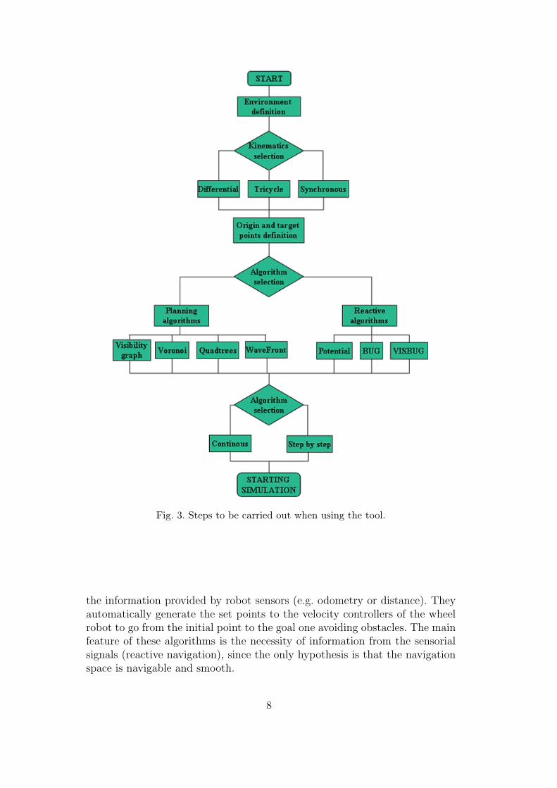
Fig. 3. Steps to be carried out when using the tool.

the information provided by robot sensors (e.g. odometry or distance). Theyautomatically generate the set points to the velocity controllers of the wheelrobot to go from the initial point to the goal one avoiding obstacles. The mainfeature of these algorithms is the necessity of information from the sensorialsignals (reactive navigation), since the only hypothesis is that the navigationspace is navigable and smooth.

8

4.1 Global algorithms

The first stage when using global algorithms consists in obtaining all possiblecollision-free paths, sometimes starting with the calculation of the convex hullfor the obstacles, and augmenting the resulting shapes according to the robotdimensions. In order to obtain all possible paths from the initial to the goalpoints, several algorithms can be used [17], [20], [2], as those implemented inthe interactive tool (see Table 1):

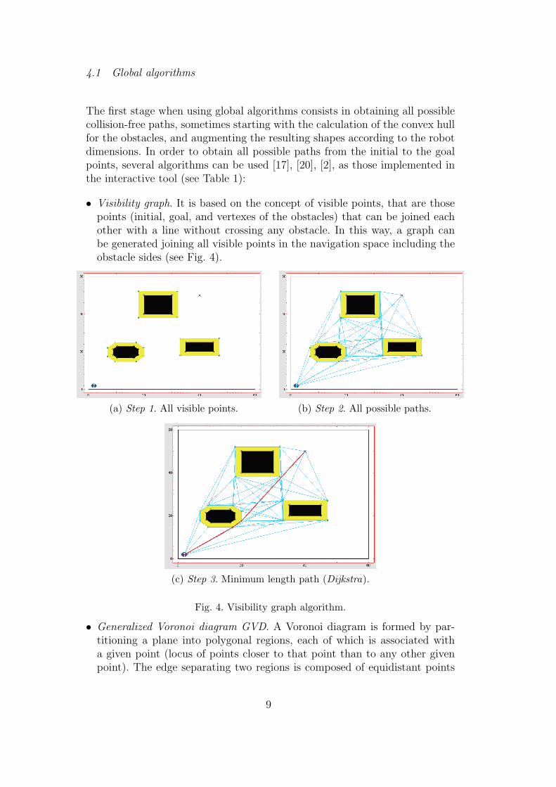
• Visibility graph. It is based on the concept of visible points, that are thosepoints (initial, goal, and vertexes of the obstacles) that can be joined eachother with a line without crossing any obstacle. In this way, a graph canbe generated joining all visible points in the navigation space including theobstacle sides (see Fig. 4).

(a) Step 1. All visible points. (b) Step 2. All possible paths.

(c) Step 3. Minimum length path (Dijkstra).

Fig. 4. Visibility graph algorithm.

• Generalized Voronoi diagram GVD. A Voronoi diagram is formed by par-titioning a plane into polygonal regions, each of which is associated witha given point (locus of points closer to that point than to any other givenpoint). The edge separating two regions is composed of equidistant points

9

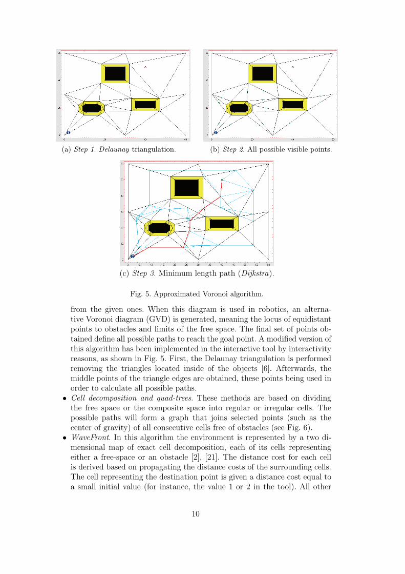
(a) Step 1. Delaunay triangulation. (b) Step 2. All possible visible points.

(c) Step 3. Minimum length path (Dijkstra).

Fig. 5. Approximated Voronoi algorithm.

from the given ones. When this diagram is used in robotics, an alterna-tive Voronoi diagram (GVD) is generated, meaning the locus of equidistantpoints to obstacles and limits of the free space. The final set of points ob-tained define all possible paths to reach the goal point. A modified version ofthis algorithm has been implemented in the interactive tool by interactivityreasons, as shown in Fig. 5. First, the Delaunay triangulation is performedremoving the triangles located inside of the objects [6]. Afterwards, themiddle points of the triangle edges are obtained, these points being used inorder to calculate all possible paths.

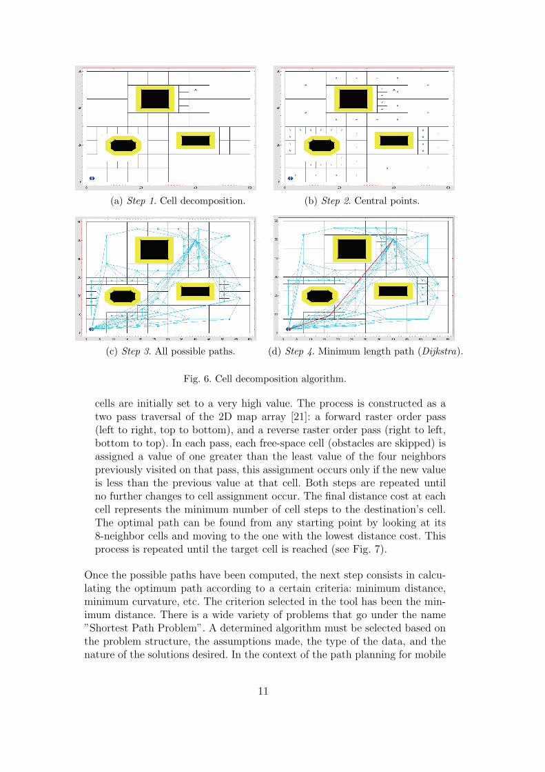
• Cell decomposition and quad-trees. These methods are based on dividingthe free space or the composite space into regular or irregular cells. Thepossible paths will form a graph that joins selected points (such as thecenter of gravity) of all consecutive cells free of obstacles (see Fig. 6).

• WaveFront. In this algorithm the environment is represented by a two di-mensional map of exact cell decomposition, each of its cells representingeither a free-space or an obstacle [2], [21]. The distance cost for each cellis derived based on propagating the distance costs of the surrounding cells.The cell representing the destination point is given a distance cost equal toa small initial value (for instance, the value 1 or 2 in the tool). All other

10

(a) Step 1. Cell decomposition. (b) Step 2. Central points.

(c) Step 3. All possible paths. (d) Step 4. Minimum length path (Dijkstra).

Fig. 6. Cell decomposition algorithm.

cells are initially set to a very high value. The process is constructed as atwo pass traversal of the 2D map array [21]: a forward raster order pass(left to right, top to bottom), and a reverse raster order pass (right to left,bottom to top). In each pass, each free-space cell (obstacles are skipped) isassigned a value of one greater than the least value of the four neighborspreviously visited on that pass, this assignment occurs only if the new valueis less than the previous value at that cell. Both steps are repeated untilno further changes to cell assignment occur. The final distance cost at eachcell represents the minimum number of cell steps to the destination’s cell.The optimal path can be found from any starting point by looking at its8-neighbor cells and moving to the one with the lowest distance cost. Thisprocess is repeated until the target cell is reached (see Fig. 7).

Once the possible paths have been computed, the next step consists in calcu-lating the optimum path according to a certain criteria: minimum distance,minimum curvature, etc. The criterion selected in the tool has been the min-imum distance. There is a wide variety of problems that go under the name”Shortest Path Problem”. A determined algorithm must be selected based onthe problem structure, the assumptions made, the type of the data, and thenature of the solutions desired. In the context of the path planning for mobile

11

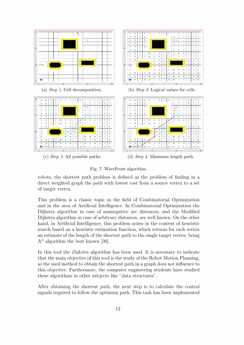
(a) Step 1. Cell decomposition. (b) Step 2. Logical values for cells.

(c) Step 3. All possible paths. (d) Step 4. Minimum length path.

Fig. 7. WaveFront algorithm.

robots, the shortest path problem is defined as the problem of finding in adirect weighted graph the path with lowest cost from a source vertex to a setof target vertex.

This problem is a classic topic in the field of Combinatorial Optimizationand in the area of Artificial Intelligence. In Combinatorial Optimization theDijkstra algorithm in case of nonnegative arc distances, and the ModifiedDijkstra algorithm in case of arbitrary distances, are well known. On the otherhand, in Artificial Intelligence, this problem arises in the context of heuristicsearch based on a heuristic estimation function, which returns for each vertexan estimate of the length of the shortest path to the single target vertex, beingA* algorithm the best known [30].

In this tool the Dijkstra algorithm has been used. It is necessary to indicatethat the main objective of this tool is the study of the Robot Motion Planning,so the used method to obtain the shortest path in a graph does not influence tothis objective. Furthermore, the computer engineering students have studiedthese algorithms in other subjects like ”data structures”.

After obtaining the shortest path, the next step is to calculate the controlsignals required to follow the optimum path. This task has been implemented

12

using the pure pursuit method due to its simplicity and easy understanding bythe students, although other strategies such as constrained predictive control[11] could be also used for these purposes.

4.1.1 Pure Pursuit

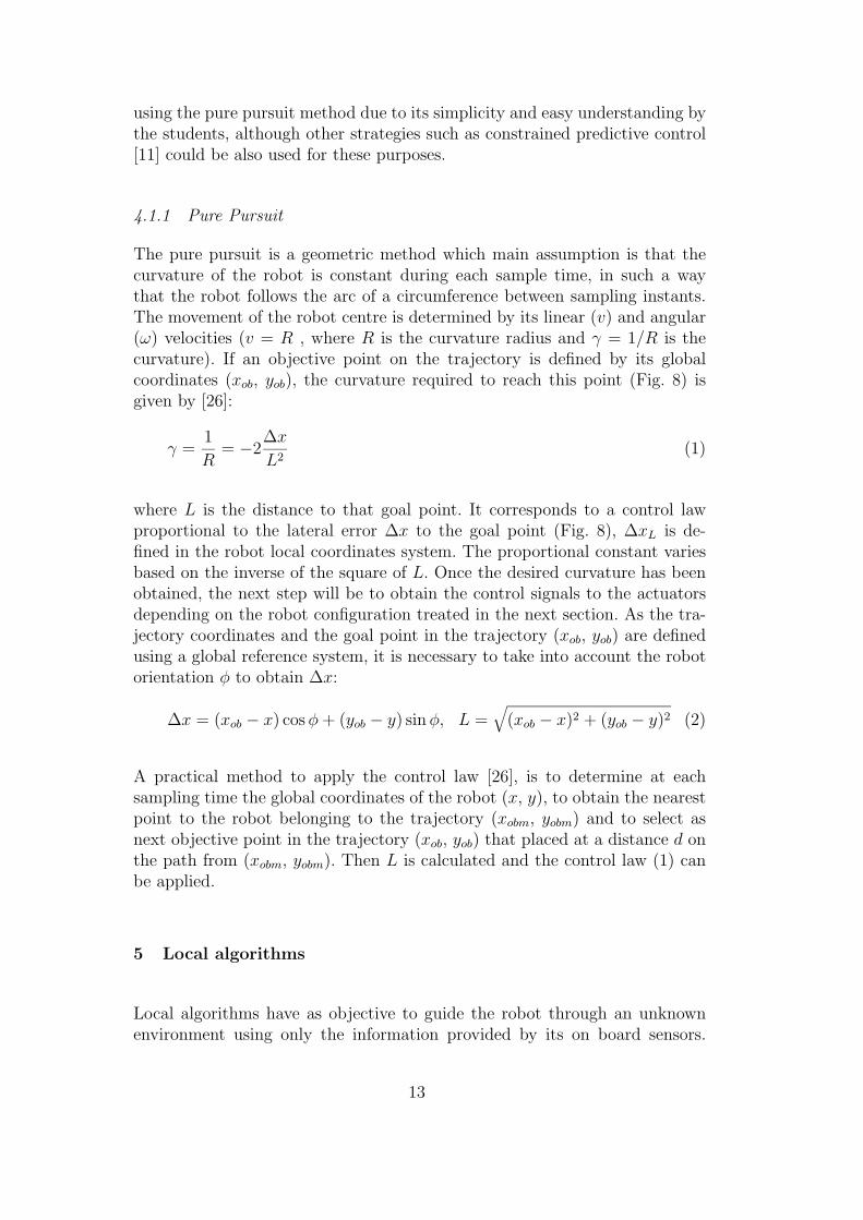
The pure pursuit is a geometric method which main assumption is that thecurvature of the robot is constant during each sample time, in such a waythat the robot follows the arc of a circumference between sampling instants.The movement of the robot centre is determined by its linear (v) and angular(ω) velocities (v = R , where R is the curvature radius and γ = 1/R is thecurvature). If an objective point on the trajectory is defined by its globalcoordinates (xob, yob), the curvature required to reach this point (Fig. 8) isgiven by [26]:

γ =1

R= −2

Δx

L2(1)

where L is the distance to that goal point. It corresponds to a control lawproportional to the lateral error Δx to the goal point (Fig. 8), ΔxL is de-fined in the robot local coordinates system. The proportional constant variesbased on the inverse of the square of L. Once the desired curvature has beenobtained, the next step will be to obtain the control signals to the actuatorsdepending on the robot configuration treated in the next section. As the tra-jectory coordinates and the goal point in the trajectory (xob, yob) are definedusing a global reference system, it is necessary to take into account the robotorientation φ to obtain Δx:

Δx = (xob − x) cos φ + (yob − y) sin φ, L =√

(xob − x)2 + (yob − y)2 (2)

A practical method to apply the control law [26], is to determine at eachsampling time the global coordinates of the robot (x, y), to obtain the nearestpoint to the robot belonging to the trajectory (xobm, yobm) and to select asnext objective point in the trajectory (xob, yob) that placed at a distance d onthe path from (xobm, yobm). Then L is calculated and the control law (1) canbe applied.

5 Local algorithms

Local algorithms have as objective to guide the robot through an unknownenvironment using only the information provided by its on board sensors.

13

(a) Control law application. (b) Calculating the new objective point.

Fig. 8. Pure pursuit method.

The main advantages against global algorithms are that the required com-putational power is much smaller and are easier to implement. The maindrawback is that in general, the solution (reaching the goal point) cannot beguaranteed, even if this exists (only some types of methods like BUG ones canprovide some figures regarding convergence). The following local algorithmshave been considered in the tool [2], [17], [20] (see Table 1):

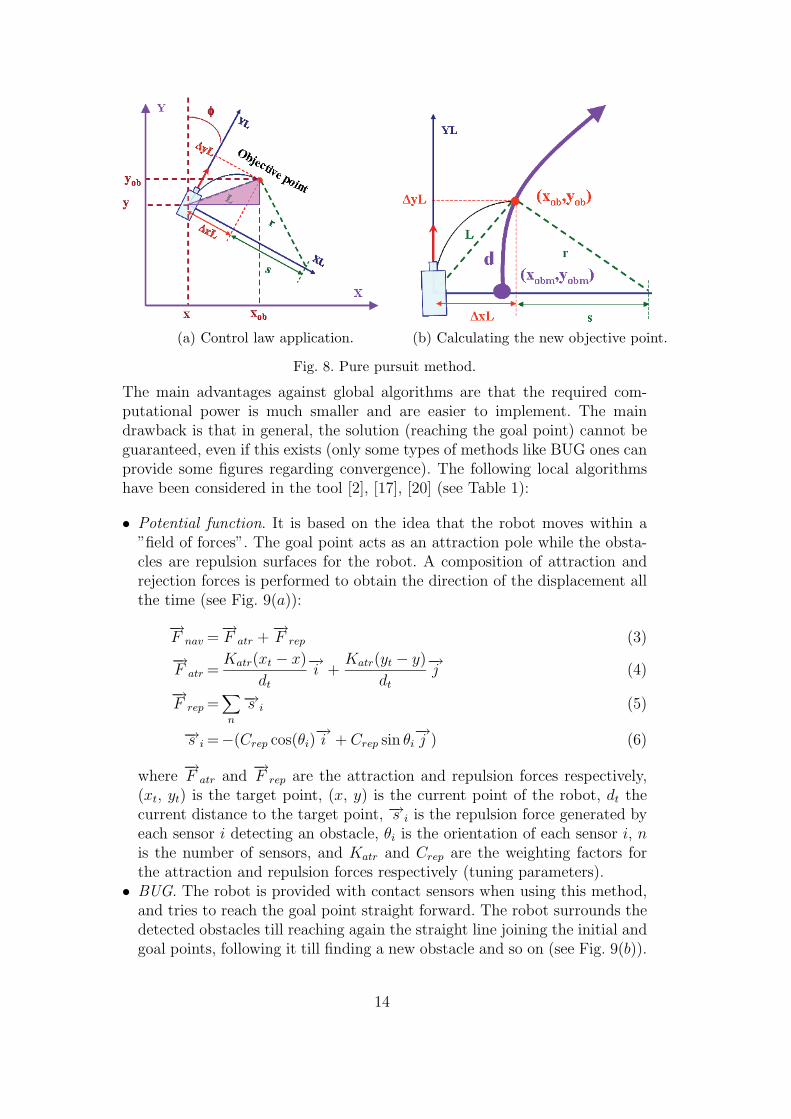
• Potential function. It is based on the idea that the robot moves within a”field of forces”. The goal point acts as an attraction pole while the obsta-cles are repulsion surfaces for the robot. A composition of attraction andrejection forces is performed to obtain the direction of the displacement allthe time (see Fig. 9(a)):

−→F nav =

−→F atr +

−→F rep (3)

−→F atr =

Katr(xt − x)

dt

−→i +

Katr(yt − y)

dt

−→j (4)

−→F rep =

∑n

−→s i (5)

−→s i =−(Crep cos(θi)−→i + Crep sin θi

−→j ) (6)

where−→F atr and

−→F rep are the attraction and repulsion forces respectively,

(xt, yt) is the target point, (x, y) is the current point of the robot, dt thecurrent distance to the target point, −→s i is the repulsion force generated byeach sensor i detecting an obstacle, θi is the orientation of each sensor i, nis the number of sensors, and Katr and Crep are the weighting factors forthe attraction and repulsion forces respectively (tuning parameters).

• BUG. The robot is provided with contact sensors when using this method,and tries to reach the goal point straight forward. The robot surrounds thedetected obstacles till reaching again the straight line joining the initial andgoal points, following it till finding a new obstacle and so on (see Fig. 9(b)).

14

• VISBUG. It is a modification to the BUG algorithm but using finite rangedistance sensors, in such a way that it is not necessary to contact with theobstacles. So, direction changes are performed in advance and non-convexzones of the obstacles are avoided (see Fig. 9(c)).

It is also possible to combine global and local algorithms: the first ones canbe used to obtain a minimum length path within a known environment andonce the path tracking has started, the local algorithms can be used to avoidcollisions with unknown obstacles or to compensate for environment imper-fections. This last option combining algorithms has not been implemented inthe interactive tool in order to facilitate the understanding of the differentalgorithms separately.

(a) Potential algorithm. (b) BUG algorithm.

(c) VISBUG algorithm.

Fig. 9. Local algorithms.

6 Robot kinematics

The implementation of the path planning and tracking tasks requires the esti-mation of the robot position in relation to the same absolute reference systemwhere the coordinates of the trajectories are defined. The kinematic models

15

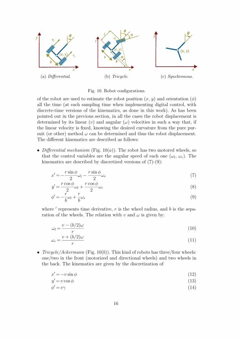
(a) Differential. (b) Tricycle. (c) Synchronous.

Fig. 10. Robot configurations.

of the robot are used to estimate the robot position (x, y) and orientation (φ)all the time (at each sampling time when implementing digital control, withdiscrete-time versions of the kinematics, as done in this work). As has beenpointed out in the previous section, in all the cases the robot displacement isdetermined by its linear (v) and angular (ω) velocities in such a way that, ifthe linear velocity is fixed, knowing the desired curvature from the pure pur-suit (or other) method ω can be determined and thus the robot displacement.The different kinematics are described as follows:

• Differential mechanism (Fig. 10(a)). The robot has two motored wheels, sothat the control variables are the angular speed of each one (ωl, ωr). Thekinematics are described by discretized versions of (7)-(9):

x′ =−r sin φ

2ωl − r sin φ

2ωr (7)

y′ =r cos φ

2ωl +

r cos φ

2ωr (8)

φ′ =−r

bωl +

r

bωr (9)

where ′ represents time derivative, r is the wheel radius, and b is the sepa-ration of the wheels. The relation with v and ω is given by:

ωl =v − (b/2)ω

r(10)

ωr =v + (b/2)ω

r(11)

• Tricycle/Ackermann (Fig. 10(b)). This kind of robots has three/four wheels:one/two in the front (motorized and directional wheels) and two wheels inthe back. The kinematics are given by the discretization of

x′ =−v sin φ (12)

y′ = v cos φ (13)

φ′ = vγ (14)

16

The control signals in this configuration are the direction angle α and theangular velocity of the directional wheel ωt, given by:

ωt =vt

r=

√v2 + ω2l2

r(15)

γ =tan α

l(16)

where l is the robot length and r is the radius of the directional wheel.• Synchronous (Fig. 10(c)). It contains transmissions to allow positioning all

the wheels with an angular speed ω simultaneously, and moving the robotwith a linear speed v. The kinematics is given by

x′ =−v sin φ (17)

y′ = v cos φ (18)

φ′ = ω (19)

with the angular speed ω being the control signal.

7 Illustrative examples

Several examples are shown in this section to demonstrate the main capabili-ties of the tool, although as has been pointed out, its main characteristic − theinteractivity − is difficult to be reflected in a written text. Nevertheless, someof the advantages of the application are shown below. The reader is cordiallyinvited to visit the Web site [12] to experience the interactive features of thetool.

7.1 Global algorithms

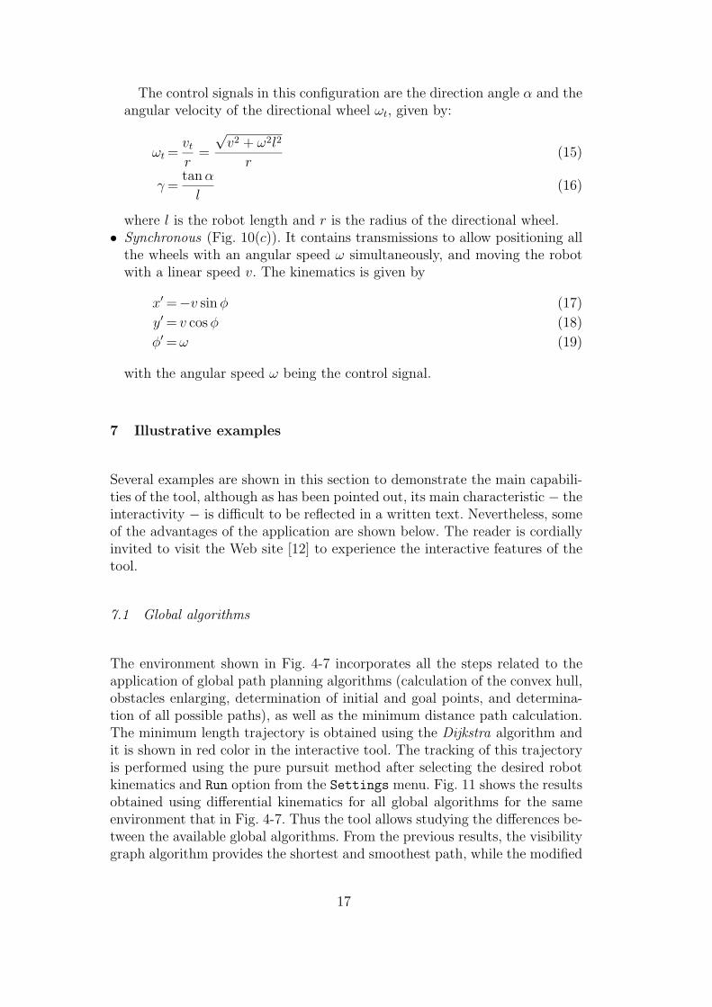
The environment shown in Fig. 4-7 incorporates all the steps related to theapplication of global path planning algorithms (calculation of the convex hull,obstacles enlarging, determination of initial and goal points, and determina-tion of all possible paths), as well as the minimum distance path calculation.The minimum length trajectory is obtained using the Dijkstra algorithm andit is shown in red color in the interactive tool. The tracking of this trajectoryis performed using the pure pursuit method after selecting the desired robotkinematics and Run option from the Settings menu. Fig. 11 shows the resultsobtained using differential kinematics for all global algorithms for the sameenvironment that in Fig. 4-7. Thus the tool allows studying the differences be-tween the available global algorithms. From the previous results, the visibilitygraph algorithm provides the shortest and smoothest path, while the modified

17

Voronoi algorithm the longest and most angular one. However, from a safetypoint of view (distance to obstacles), the Voronoi and wave front algorithmsprovide the best results.

(a) Visibility graph. (b) Voronoi diagram.

(c) Cell decomposition. (d) WaveFront.

Fig. 11. Tracking examples for global algorithms.

7.2 Obstacles insertion

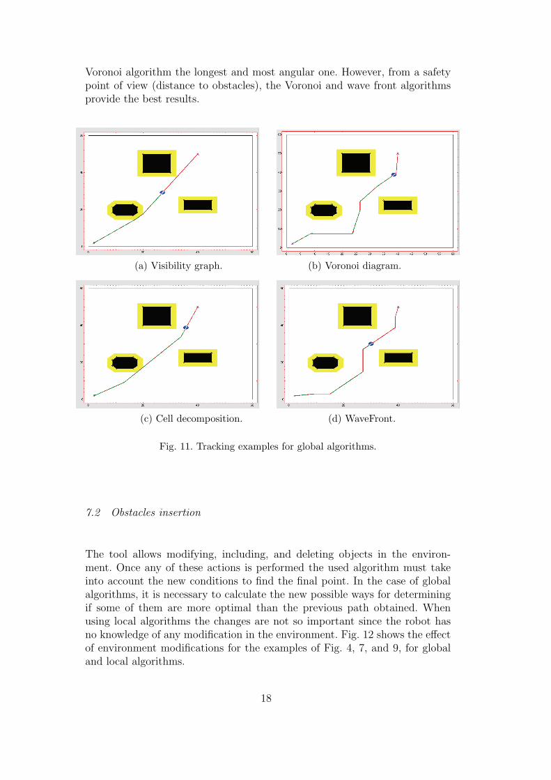
The tool allows modifying, including, and deleting objects in the environ-ment. Once any of these actions is performed the used algorithm must takeinto account the new conditions to find the final point. In the case of globalalgorithms, it is necessary to calculate the new possible ways for determiningif some of them are more optimal than the previous path obtained. Whenusing local algorithms the changes are not so important since the robot hasno knowledge of any modification in the environment. Fig. 12 shows the effectof environment modifications for the examples of Fig. 4, 7, and 9, for globaland local algorithms.

18

(a) Visibility graph. (b) WaveFront.

(c) BUG. (d) Potential.

Fig. 12. Effect of environment modification in different algorithms.

7.3 Constraints over the control signals and kinematics

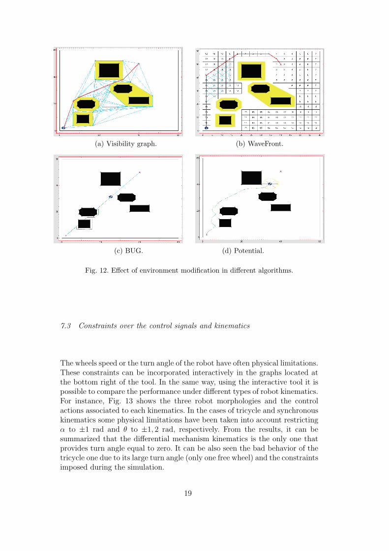
The wheels speed or the turn angle of the robot have often physical limitations.These constraints can be incorporated interactively in the graphs located atthe bottom right of the tool. In the same way, using the interactive tool it ispossible to compare the performance under different types of robot kinematics.For instance, Fig. 13 shows the three robot morphologies and the controlactions associated to each kinematics. In the cases of tricycle and synchronouskinematics some physical limitations have been taken into account restrictingα to ±1 rad and θ to ±1, 2 rad, respectively. From the results, it can besummarized that the differential mechanism kinematics is the only one thatprovides turn angle equal to zero. It can be also seen the bad behavior of thetricycle one due to its large turn angle (only one free wheel) and the constraintsimposed during the simulation.

19

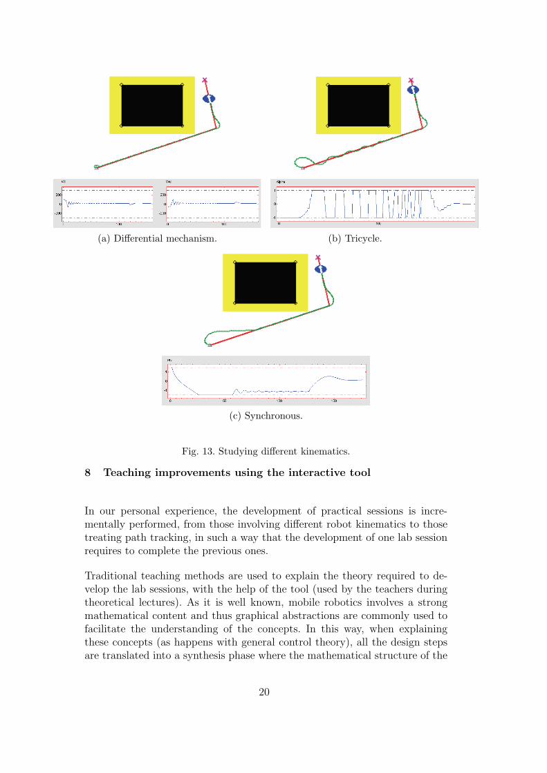
(a) Differential mechanism. (b) Tricycle.

(c) Synchronous.

Fig. 13. Studying different kinematics.

8 Teaching improvements using the interactive tool

In our personal experience, the development of practical sessions is incre-mentally performed, from those involving different robot kinematics to thosetreating path tracking, in such a way that the development of one lab sessionrequires to complete the previous ones.

Traditional teaching methods are used to explain the theory required to de-velop the lab sessions, with the help of the tool (used by the teachers duringtheoretical lectures). As it is well known, mobile robotics involves a strongmathematical content and thus graphical abstractions are commonly used tofacilitate the understanding of the concepts. In this way, when explainingthese concepts (as happens with general control theory), all the design stepsare translated into a synthesis phase where the mathematical structure of the

20

problem is determined and after, an analysis phase has to be carried out toanalyze the results. This iterative process performed in two phases has beenmerged into one in the interactive tool.

The tool is also used by the students to analyze and compare the results withthose of laboratory sessions. The implementation of the algorithms in theselab sessions is performed in Matlab/Simulink (alternatively in C++ or Java)and the proposed lab sessions for a typical 60 hours course are (30 hours forlab sessions):

• Lab session 1. Learning and implementation of different robot kinematics:differential, tricycle, and synchronous. A discretized version of the algo-rithms is implemented, without incorporating dynamics.

• Lab session 2. The objective of this session is to implement and test the purepursuit method using as robot simulator the kinematic model developed inthe previous lab session.

• Lab session 3. The objective is the implementation of one global algorithm(visibility graph, GVD or quadtrees) and one local method (potential, BUG,VISBUG) selected by the lecturer.

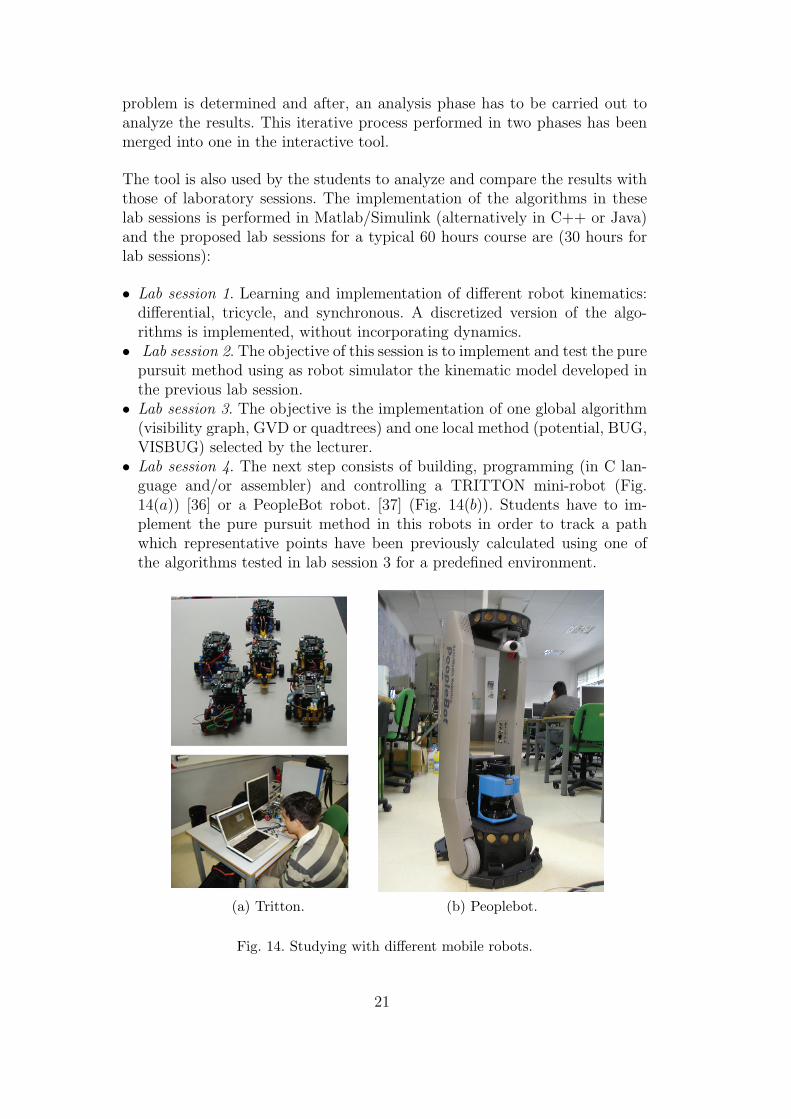
• Lab session 4. The next step consists of building, programming (in C lan-guage and/or assembler) and controlling a TRITTON mini-robot (Fig.14(a)) [36] or a PeopleBot robot. [37] (Fig. 14(b)). Students have to im-plement the pure pursuit method in this robots in order to track a pathwhich representative points have been previously calculated using one ofthe algorithms tested in lab session 3 for a predefined environment.

(a) Tritton. (b) Peoplebot.

Fig. 14. Studying with different mobile robots.

21

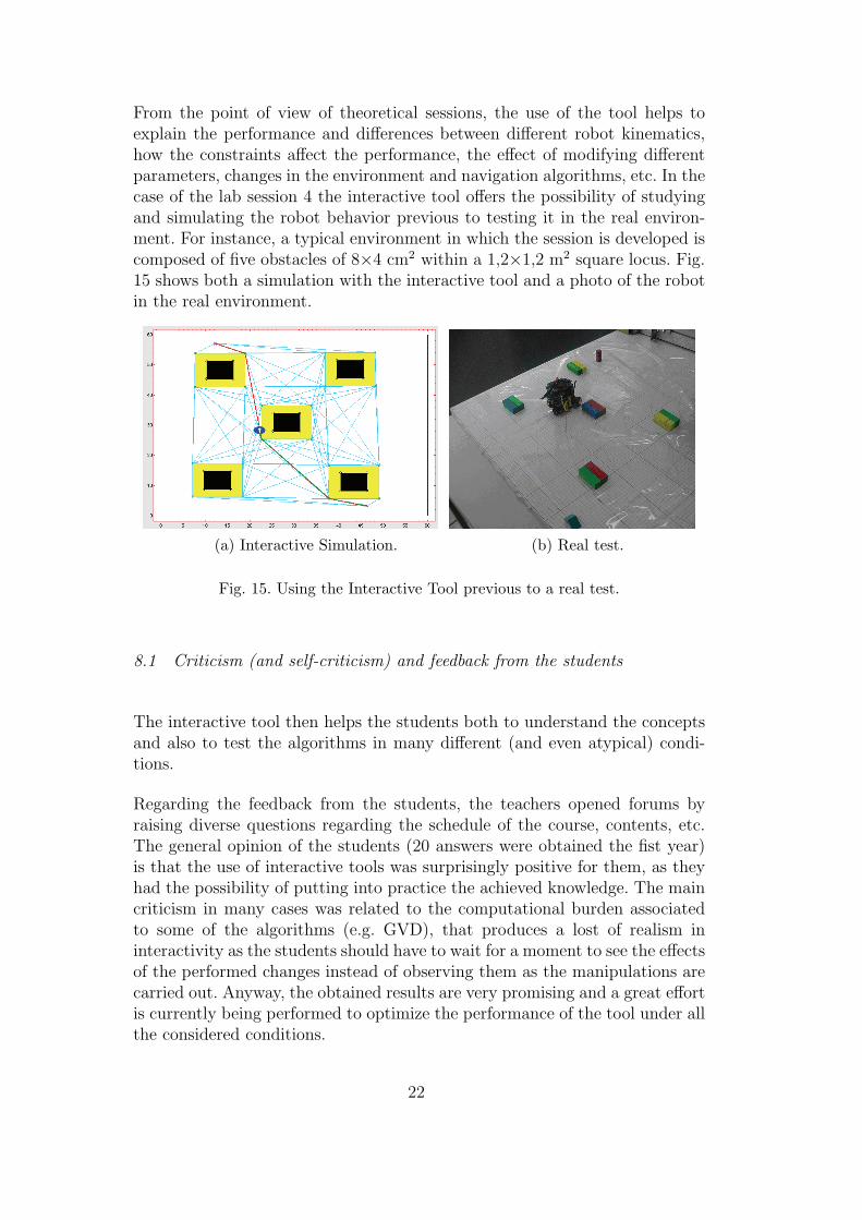
From the point of view of theoretical sessions, the use of the tool helps toexplain the performance and differences between different robot kinematics,how the constraints affect the performance, the effect of modifying differentparameters, changes in the environment and navigation algorithms, etc. In thecase of the lab session 4 the interactive tool offers the possibility of studyingand simulating the robot behavior previous to testing it in the real environ-ment. For instance, a typical environment in which the session is developed iscomposed of five obstacles of 8×4 cm2 within a 1,2×1,2 m2 square locus. Fig.15 shows both a simulation with the interactive tool and a photo of the robotin the real environment.

(a) Interactive Simulation. (b) Real test.

Fig. 15. Using the Interactive Tool previous to a real test.

8.1 Criticism (and self-criticism) and feedback from the students

The interactive tool then helps the students both to understand the conceptsand also to test the algorithms in many different (and even atypical) condi-tions.

Regarding the feedback from the students, the teachers opened forums byraising diverse questions regarding the schedule of the course, contents, etc.The general opinion of the students (20 answers were obtained the fist year)is that the use of interactive tools was surprisingly positive for them, as theyhad the possibility of putting into practice the achieved knowledge. The maincriticism in many cases was related to the computational burden associatedto some of the algorithms (e.g. GVD), that produces a lost of realism ininteractivity as the students should have to wait for a moment to see the effectsof the performed changes instead of observing them as the manipulations arecarried out. Anyway, the obtained results are very promising and a great effortis currently being performed to optimize the performance of the tool under allthe considered conditions.

22

9 Conclusions and future work

This work shows an interactive tool aimed at helping the students to under-stand the basis of mobile robot navigation and letting them modifying differentcharacteristics such as robot kinematics, kind of path planning algorithm, theshape of the obstacles, etc. Typical robotics simulation tools are expensive andthus it is difficult to have many licenses for the students. The same applies toreal robots. The use of interactive tools as that presented in this paper consti-tutes an alternative to classical teaching tools. The developed interactive toolis free and it can be obtained in English and in Spanish including also a cou-ple of relevant tutorials [12]. It is available at http://www.calerga.com/ orhttp://aer.ual.es/mrit/ and it can run under Windows, Linux, and MACoperating systems.

Future works will include:

• Improving the computational efficiency of some of the implemented algo-rithms.

• The incorporation of new path tracking algorithms, such as constrained pre-dictive control, as the authors have much experience in this kind of controltechniques [11] and may explicitly take into account constraints acting onthe control signals.

• Multivariable control for velocity and orientation.• Inclusion of multiple robots.• Development of a virtual lab by allowing its use through Internet and pos-

sible adaptation to a remote lab using in this case Sysquake Remote.

Acknowledgments

This work was supported by the Spanish CICYT and FEDER funds undergrants DPI2004-07444-C04-04 and DPI2004-01804. The authors would like tothank Mr. Oliver Rodrıguez Lopez, Mr. Manuel Pasamontes, and Dr. YvesPiguet for their help and suggestions.

References

[1] S. Athanasiou, I. Poulakis, P. Tsanakas, N. Koziris, TALOS: An interactiveWeb-enabled educational environment on mobile robot technology, in:Proceedings of 10th Mediterranean Electrotechnical Conference I, Madrid(Spain), 2000, pp. 387-395.

23

[2] H. Choset, K. M. Lynch, S. Hutchinson, G. Kantor, W. Burgard, L. Kavraki,Principles of Robot Motion. Theory, Algorithms, and Implementations, TheMIT Press, 2005.

[3] C. Cosma, M. Confente, D. Botturi, P. Fiorini, Laboratory tools for toboticsand automation education, in: Proceedings of IEEE International Conferenceon Robotics and Automation, Tapei (Taiwian), vol. 3, 2003, pp. 3303-3308.

[4] F. Dai, Integrated planning of robotic applications in a graphic-interactiveenvironment, Robotics and Autonomous Systems 8 (1991) 311-322.

[5] A. G. Demitriou, A. H. Lambert, Virtual environments for robotics education:an extensible object-orientation platform, IEEE Robotics and Automation 12(4) (2006) 75-91.

[6] M. de Berg, M. van Kreveld, M. Overmars, O. Schwarzkoph, Computationalgeometry: algorithms and applications, Springer-Verlag, 2000.

[7] S. Dormido, Control learning: present and future, Annual Reviews in Control28 (1) (2004) 115–136.

[8] P. Ehlert, The use of artificial intelligence in autonomous mobile robots,Research Report, Knowledge Based Systems Group, Delft University ofTechnology, 1999.

[9] A. Elnagar, L. Lulu, A global path planning Java-based system for autonomousmobile robots, Science of Computer Programming 53 (1) (2004) 107-122.

[10] A. Elnagar, L. Lulu, A visual tool for computer supported learning: The robotmotion planning example, Computers and Education, in press (corrected proofavailable from 2005).

[11] J. L. Guzman, M. Berenguel, S. Dormido, Interactive teaching of constrainedgeneralized predictive control, IEEE Control Systems Magazine 25 (2) (2005)79-85, available: http://aer.ual.es/siso-gpcit/.

[12] J. L. Guzman, O. Lopez, M. Berenguel, F. Rodrıguez, S. Dormido, MRIT- Mobile Robotics Interactive Tool, UAL/UNED Internal Report, available:http://aer.ual.es/mrit/ and http://www.calerga.com, 2005.

[13] J. L. Guzman, F. Rodrıguez, M. Berenguel, S. Dormido, MRIT: Mobile robotinteractive tool, in: Proceedings of the IFAC Workshop on Internet-BasedControl Education IBCE04, Grenoble (France), 2004.

[14] J. L. Guzman, Interactive control system design, Ph.D. Thesis, Deparment ofLenguajes y Computacion, University of Almerıa, Spain, 2006.

[15] B. Heck (editor), Enhancing classical control education via interactive GUIdesign, IEEE Control System Magazine 19 (3) (1999) 35-58.

[16] J. Hrabec, Autonomous mobile robotics toolbox SIMROBOT, avilable:http://www.uamt.feec.vutbr.cz/robotics/, 2000.

24

[17] M. Jenkin, G. Dudek, Computational principles of mobile robotics, CambridgeUniversity Press, 2000.

[18] M. Johansson, M. Gafvert, K. Astrom, Interactive tools for education inautomatic control, IEEE Control Systems Magazine 18 (3) (1998) 33-40.

[19] R. Kelly, S. Dormido, C. Monroy, E. Dıaz, Learning control of robotmanipulators by interactive simulation, Robotica 23 (2005) 515-520.

[20] J. C. Latombe, Robot motion planning, Kluwer Academic Publishers, 1991.

[21] M. Marouqi, R. Jarvis, Covert robotics: covert path planning in unknownenvironments, in: Proceedings of the Australasian Conference on Robotics andAutomationCanberra (Australia), 2003.

[22] The MathWorks Inc., Using Matlab. The language of technical computing, 2002.

[23] I. Maza, A. Ollero, HEMERO: A MATLAB-Simulink toolbox for robotics,in: Proceedings of the 1st Workshop on Robotics Education and Training,Weingarten (Germany), 2001.

[24] O. Michel, Khepera simulator version 2.0, available:http://diwww.epfl.ch/lami/team/michel/khep-sim/SIM2.tar.gz, 1999.

[25] U. Nehmzow, Mobile robotics, Springer, 2003.

[26] A. Ollero, Robotica. Manipuladores y robots moviles (in Spanish), Marcombo,2001.

[27] T. Petrinic, E. Ivanjko, I. Petrovic, An interactive system for mobile robotnavigation, in: Proceedings of the 5th International Workshop on Robot Motionand Control, Balatonfured, Lake Balaton (Hungary), 2005.

[28] T. Petrinic, E. Ivanjko, I. Petrovic, AMORsim- A mobile robot simulator forMatlab, in: Proceedings of the 15th International Workshop on Robotics inAlpe-Adria-Danube Region, Balatonfured, Lake Balaton (Hungary), 2006.

[29] Y. Piguet, SysQuake 3 user manual, Calerga Sarl, Lausanne (Switzerland), 2004.

[30] W. Pijls, A. Kolen, A general framework for shortest path algorithms, technicalReport 92-08, University of Rotterdam (Holland), 2000.

[31] J. Sanchez, S. Dormido, F. Esquembre, The learning of control concepts usinginteractive tools, Computer Applications in Engineering Education 13 (1)(2005) 84-98.

[32] J. Sanchez, F. Morilla, S. Dormido, J. Aranda, P. Ruiperez, Virtual controllab using Java and Matlab: A qualitative approach, IEEE Control SystemsMagazine 22 (2) (2002) 8-20.

[33] D. Srinivasagupta, B. Joseph, An Internet-mediated process control laboratory,IEEE Control System Magazine 23 (1) (2003) 11-18.

25

[34] R. T. Vaughan, Stage: a multiple robot simulator, Technical Report IRIS-00-394, Institute for Robotics and Intelligent Systems, University of SouthernCalifornia, available: ftp://robot.usc.edu/pub/stage/stage manual.ps.gz, 2000.

[35] B. Wittenmark, H. Hagglund, M. Johansson, Dynamic pictures and interactivelearning, IEEE Control Systems Magazine 18 (3) (1998) 26-32.

[36] Microbotica S.L., available: http://www.microbotica.com/.

[37] Mobile robots company, available: http://www.activrobots.com/.

26

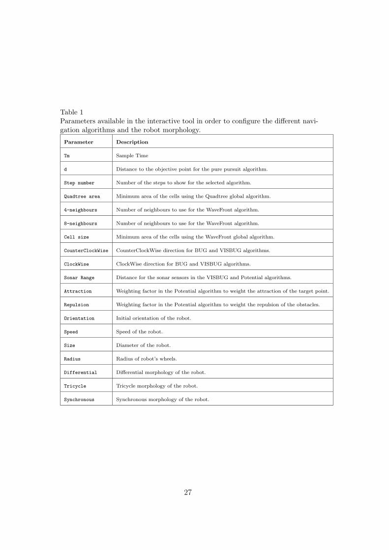
Table 1Parameters available in the interactive tool in order to configure the different navi-gation algorithms and the robot morphology.

Parameter Description

Tm Sample Time

d Distance to the objective point for the pure pursuit algorithm.

Step number Number of the steps to show for the selected algorithm.

Quadtree area Minimum area of the cells using the Quadtree global algorithm.

4-neighbours Number of neighbours to use for the WaveFront algorithm.

8-neighbours Number of neighbours to use for the WaveFront algorithm.

Cell size Minimum area of the cells using the WaveFront global algorithm.

CounterClockWise CounterClockWise direction for BUG and VISBUG algorithms.

ClockWise ClockWise direction for BUG and VISBUG algorithms.

Sonar Range Distance for the sonar sensors in the VISBUG and Potential algorithms.

Attraction Weighting factor in the Potential algorithm to weight the attraction of the target point.

Repulsion Weighting factor in the Potential algorithm to weight the repulsion of the obstacles.

Orientation Initial orientation of the robot.

Speed Speed of the robot.

Size Diameter of the robot.

Radius Radius of robot’s wheels.

Differential Differential morphology of the robot.

Tricycle Tricycle morphology of the robot.

Synchronous Synchronous morphology of the robot.

27

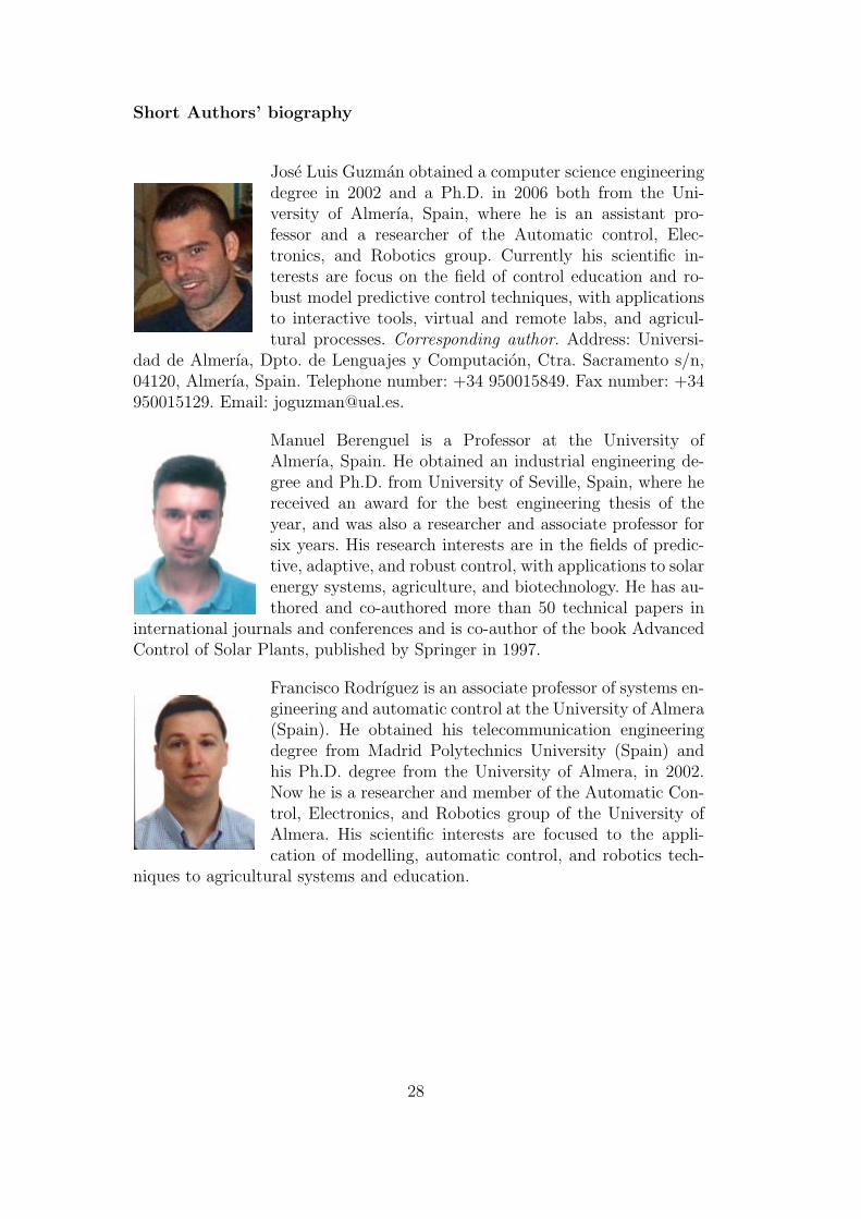
Short Authors’ biography

Jose Luis Guzman obtained a computer science engineeringdegree in 2002 and a Ph.D. in 2006 both from the Uni-versity of Almerıa, Spain, where he is an assistant pro-fessor and a researcher of the Automatic control, Elec-tronics, and Robotics group. Currently his scientific in-terests are focus on the field of control education and ro-bust model predictive control techniques, with applicationsto interactive tools, virtual and remote labs, and agricul-tural processes. Corresponding author. Address: Universi-

dad de Almerıa, Dpto. de Lenguajes y Computacion, Ctra. Sacramento s/n,04120, Almerıa, Spain. Telephone number: +34 950015849. Fax number: +34950015129. Email: joguzman@ual.es.

Manuel Berenguel is a Professor at the University ofAlmerıa, Spain. He obtained an industrial engineering de-gree and Ph.D. from University of Seville, Spain, where hereceived an award for the best engineering thesis of theyear, and was also a researcher and associate professor forsix years. His research interests are in the fields of predic-tive, adaptive, and robust control, with applications to solarenergy systems, agriculture, and biotechnology. He has au-thored and co-authored more than 50 technical papers in

international journals and conferences and is co-author of the book AdvancedControl of Solar Plants, published by Springer in 1997.

Francisco Rodrıguez is an associate professor of systems en-gineering and automatic control at the University of Almera(Spain). He obtained his telecommunication engineeringdegree from Madrid Polytechnics University (Spain) andhis Ph.D. degree from the University of Almera, in 2002.Now he is a researcher and member of the Automatic Con-trol, Electronics, and Robotics group of the University ofAlmera. His scientific interests are focused to the appli-cation of modelling, automatic control, and robotics tech-

niques to agricultural systems and education.

28

Sebastian Dormido holds a degree in physics from the Com-plutense University in Madrid, Spain (1968) and a Ph.D.from University of The Basque Country, Spain (1971). In1981 he was appointed professor of control engineering atthe Universidad Nacional de Educacion a Distancia. His sci-entific activities include computer control of industrial pro-cesses, model-based predictive control, robust control, andmodel and simulation of continuous processes. He has au-thored and co-authored more than 150 technical papers ininternational journals and conferences. Since 2002 to 2006

he has been President of the Spanish Association of Automatic Control CEA-IFAC.

29