Groundwater Assessment and Its Intrinsic...

International Journal of Energy and Environmental Science 2017; 2(5): 103-116

http://www.sciencepublishinggroup.com/j/ijees

doi: 10.11648/j.ijees.20170205.13

Groundwater Assessment and Its Intrinsic Vulnerability Studies Using Aquifer Vulnerability Index and GOD Methods

Olumuyiwa Olusola Falowo*, Yemisi Akindureni, Olajumoke Ojo

Department of Civil Engineering, Faculty of Engineering Technology, Rufus Giwa Polytechnic, Owo, Nigeria

Email address:

[email protected] (O. O. Falowo) *Corresponding author

To cite this article: Olumuyiwa Olusola Falowo, Yemisi Akindureni, Olajumoke Ojo. Groundwater Assessment and Its Intrinsic Vulnerability Studies Using

Aquifer Vulnerability Index and GOD Methods. International Journal of Energy and Environmental Science.

Vol. 2, No. 5, 2017, pp. 103-116. doi: 10.11648/j.ijees.20170205.13

Received: August 24, 2017; Accepted: September 18, 2017; Published: September 28, 2017

Abstract: Groundwater assessment and aquifer/water bearing formation vulnerability studies were carried out in Ose and

Owo Local Government areas of Ondo State, Southwestern Nigeria. The groundwater evaluation involved integrated electrical

resistivity (vertical electrical sounding), very low frequency electromagnetic, and borehole logging. Aquifer vulnerability

assessment was done using Aquifer vulnerability Index (AVI) and GOD approaches. Fifty two (52) vertical electrical

soundings (VES) data were acquired with Schlumberger array using current electrode separation (AB/2) of 1 to 225 m. The

acquired VES data were qualitatively interpreted to determine the geoelectric parameters (layer resistivity and thickness). The

geoelectric sections revealed the lithological sequence comprising topsoil, weathered layer, partly weathered/fractured

basement and fresh basement. The most occurring curve types identified are H and KH with % frequency of 30 and 26.9

respectively. The lineament density and interception maps show a low spatial variation as the lineaments are generally sparse

in the study area especially in Ose local government area; while Owo area shows a low – moderate variation. The major water

bearing units are confined/unconfined fracture basement and weathered layer composing of clay/sandy clay, clay sand and sand

aquifers (found in the southern part of the study area with thickness generally above 20 m and could be up to 60 m). However,

the fracture basement aquifer is widespread in Owo area with thickness that could up to 30 m. The depth to these water bearing

geological formation is between 1.2 m and 15.9 m. The AVI characterized the study area into “extremely low – High

vulnerability” with predominant very high vulnerability values. The GOD vulnerability model depicts that the study area is

characterized by three vulnerability zones, which are low, moderate and high vulnerable zones. According to the model, about

5% of the area is highly vulnerable while about 45% is of moderate rating, and 50% low vulnerable rating. It is highly

recommended that the least vulnerable zone should be the primary target for future groundwater development in the area in

order to ensure continuous supply of safe and potable groundwater for human consumption; and more importantly, location of

septic tanks, petroleum storage tanks, shallow subsurface piping utilities and other contaminant facilities should be confined to

low vulnerable zones.

Keywords: GOD, AVI, Vulnerability, Groundwater, Contamination, Borehole Logging

1. Introduction

Fresh water makes up only 2.5% of all the water on earth,

but not all of this water is available for human use. The water

in polar ice caps, other forms of ice and snow, soil moisture,

marshes, biological systems, and the atmosphere are not

readily available. As a result, only the 10,530,000 km³ of

groundwater, 91,000 km³ of fresh water in lakes, and the

2,120 km³ of water in rivers are considered attainable for use

and comprise a total of 10,623,120 km³. Consequently,

groundwater comprises 99% of the earth’s available fresh

water [1] and it has now become as a national treasure and

the most important natural resources. Despite its abundance,

most people still lack fresh water for daily needs in form of

drinking, domestic, municipal, industrial and irrigation

purposes. Although governments all levels are putting up

104 Olumuyiwa Olusola Falowo et al.: Groundwater Assessment and Its Intrinsic Vulnerability Studies Using

Aquifer Vulnerability Index and GOD Methods

concerted efforts in making sure this resource becomes

readily available in towns and villages in the country, but the

results are virtually infinitesimal. In addition, most of the

successful drilled boreholes are failing at a very alarming rate

[2]; while those that have not failed are highly contaminated.

Therefore there’s need to carry out comprehensive

groundwater assessment studies using integrated approach

with state-of-the-art equipment. In this vein groundwater

assessment and its vulnerability to contamination was

undertaken in Owo and Ose local government areas of Ondo

State using hydrogeological measurements, and geophysical

methods. The vulnerability of the delineated aquifer/water

bearing formation to contamination was evaluated using

Aquifer Vulnerability Index (AVI) and GOD (groundwater

occurrence/lithology overlying aquifer/depth to water table)

methods.

1.1. Description of the Project Environment

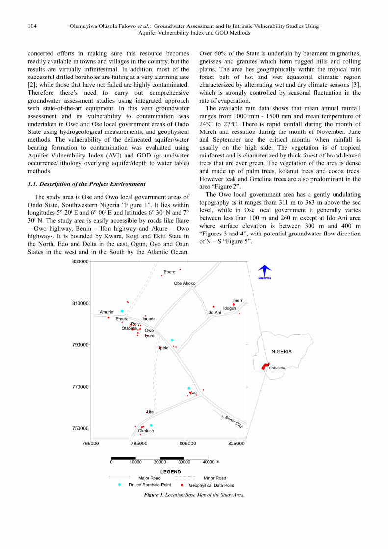
The study area is Ose and Owo local government areas of

Ondo State, Southwestern Nigeria “Figure 1”. It lies within

longitudes 5° 20ˡ E and 6° 00ˡ E and latitudes 6° 30ˡ N and 7°

30ˡ N. The study area is easily accessible by roads like Ikare

– Owo highway, Benin – Ifon highway and Akure – Owo

highways. It is bounded by Kwara, Kogi and Ekiti State in

the North, Edo and Delta in the east, Ogun, Oyo and Osun

States in the west and in the South by the Atlantic Ocean.

Over 60% of the State is underlain by basement migmatites,

gneisses and granites which form rugged hills and rolling

plains. The area lies geographically within the tropical rain

forest belt of hot and wet equatorial climatic region

characterized by alternating wet and dry climate seasons [3],

which is strongly controlled by seasonal fluctuation in the

rate of evaporation.

The available rain data shows that mean annual rainfall

ranges from 1000 mm - 1500 mm and mean temperature of

24°C to 27°C. There is rapid rainfall during the month of

March and cessation during the month of November. June

and September are the critical months when rainfall is

usually on the high side. The vegetation is of tropical

rainforest and is characterized by thick forest of broad-leaved

trees that are ever green. The vegetation of the area is dense

and made up of palm trees, kolanut trees and cocoa trees.

However teak and Gmelina trees are also predominant in the

area “Figure 2”.

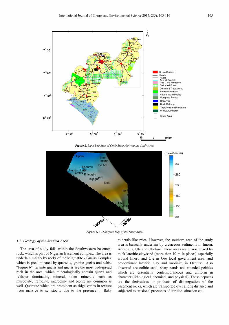
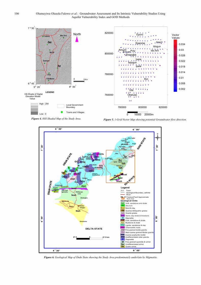
The Owo local government area has a gently undulating

topography as it ranges from 311 m to 363 m above the sea

level, while in Ose local government it generally varies

between less than 100 m and 260 m except at Ido Ani area

where surface elevation is between 300 m and 400 m

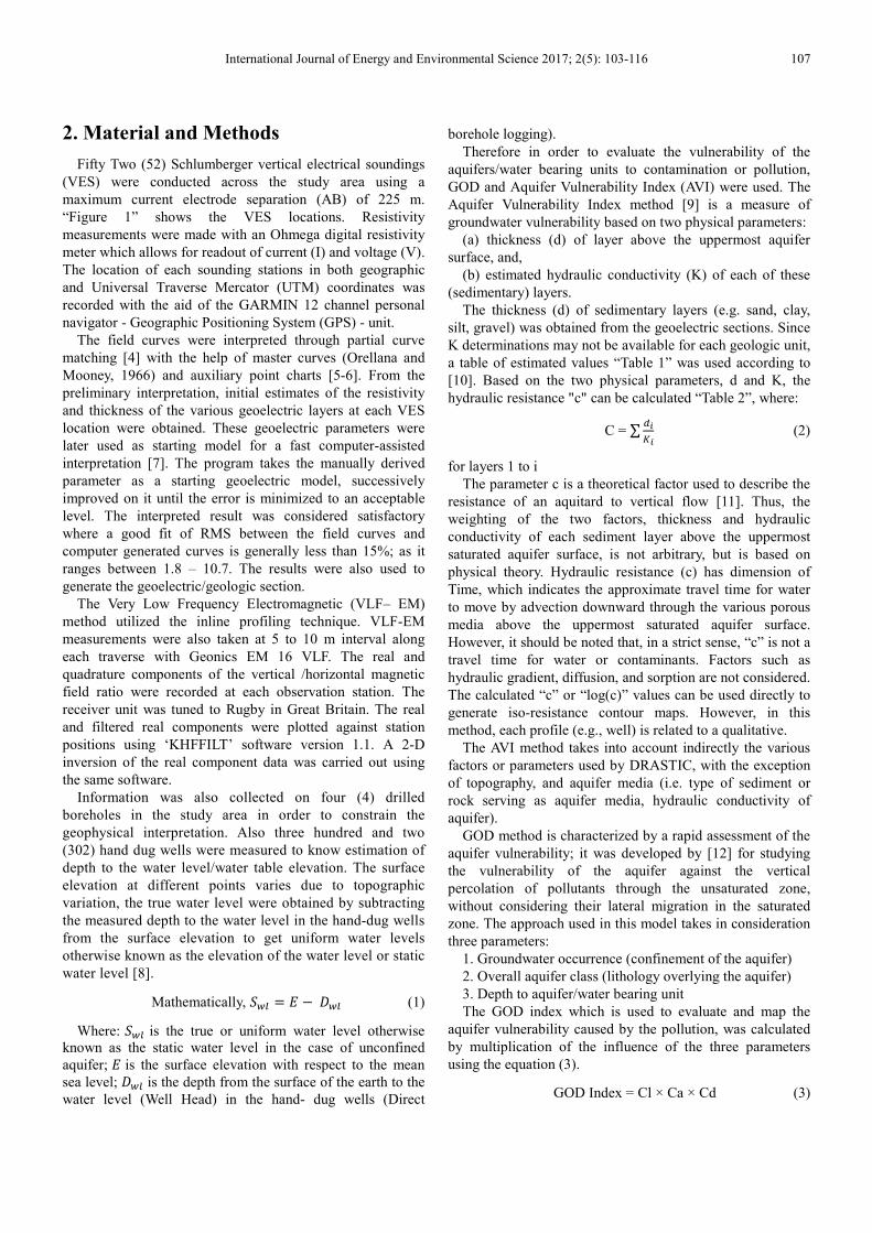
“Figures 3 and 4”, with potential groundwater flow direction

of N – S “Figure 5”.

Figure 1. Location/Base Map of the Study Area.

765000 785000 805000 825000

750000

770000

790000

810000

830000

Okeluse

Ute

Ifon

Ipele

Iyere

Amurin

Emure

OtapeteOwo

IsuadaPoly

Eporo

Ido AniIdogun

Imeri

Benin City

Oba Akoko

0 10000 20000 30000 40000 m

Major Road Minor Road

Geophysical Data PointDrilled Borehole Point

LEGEND

NIGERIA

Ondo State

International Journal of Energy and Environmental Science 2017; 2(5): 103-116 105

Figure 2. Land Use Map of Ondo State showing the Study Area.

Figure 3. 3-D Surface Map of the Study Area.

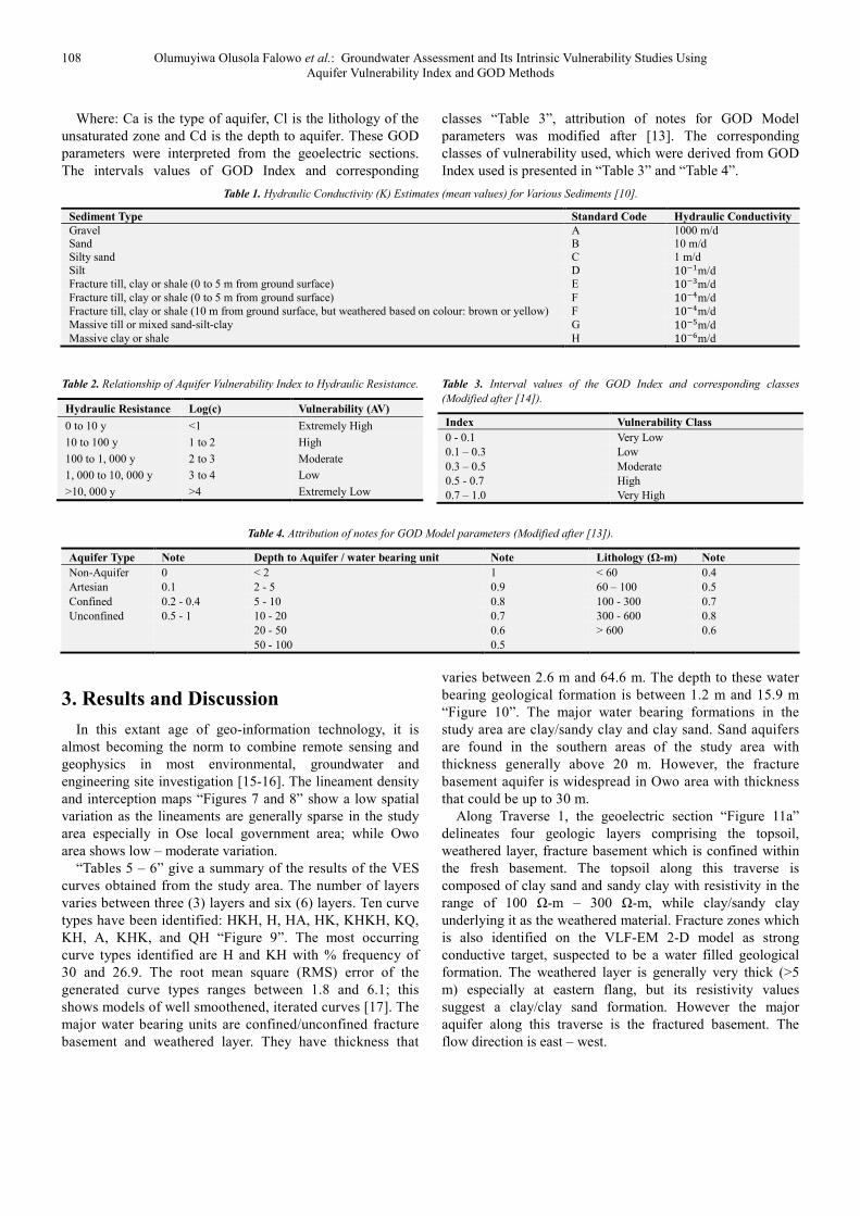
1.2. Geology of the Studied Area

The area of study falls within the Southwestern basement

rock, which is part of Nigerian Basement complex. The area is

underlain mainly by rocks of the Migmatite - Gneiss Complex

which is predominated by quartzite, granite gneiss and schist

“Figure 6”. Granite gneiss and gneiss are the most widespread

rock in the area; which mineralogically contain quartz and

feldspar dominating mineral, other minerals such as

muscovite, tremolite, microcline and biotite are common as

well. Quartzite which are prominent as ridge varies in texture

from massive to schistocity due to the presence of flaky

minerals like mica. However, the southern area of the study

area is basically underlain by cretaceous sediments in Imoru,

Arimogija, Ute and Okeluse. These areas are characterized by

thick lateritic clay/sand (more than 10 m in places) especially

around Imoru and Ute in Ose local government area; and

predominant lateritic clay and kaolinite in Okeluse. Also

observed are oolitic sand, sharp sands and rounded pebbles

which are essentially contemporaneous and uniform in

character (lithological, chemical, and physical). These deposits

are the derivatives or products of disintegration of the

basement rocks, which are transported over a long distance and

subjected to erosional processes of attrition, abrasion etc.

2000

2100

2200

1900

1800

1700

OkitipupaIrele

Ore

Ode Aye

Ilu Titun

Ile OlujiAlade

Ondo

Ifon

Oba Ile

Igbara Oke

Akure

Ilara

Iju

Ita Ogbolu

Adejubu

Uso

Owo

Supare

Ikare Akoko

1500

Undisturbed forest

Teak/Gmelina Plantation

Rock Outcrop

Reservoir

Natural Waterbodies

Forest Plantation

Urban Centres

RoadsRiversAnnual RainfallTree Crop PlantationDisturbed Forest

Dominant Trees/Wood

Mangrove Forest

30 30 km0

6 00

6 30

7 00

7 30

4 30 5 00 5 30 6 00

I

I

I

I

I I I I

Emure Ile

Study Area

1600

Oke Agbe

Ogbagi

Isua

Okeluse

Ido Ani

80

130

180

230

280

330Ido Ani

Amurin

Okeluse

Ifon

Ute

Ipele

Idogun

EporoImeri

Isijogun

Emure

Epenme

Iyere

Poly

Ehinogbe

Elevation (m)



Figure 4. Hill-Shaded Map of the Study Area.

Figure 5. 1-Grid Vector Map showing potential Groundwater flow direction.

Figure 6. Geological Map of Ondo State showing the Study Area predominately underlain by Migmatite.

6 005 20II

6 45

7 30I

I

oo

o

o

Local Government Boundary

Towns and VillagesLow : 0

High : 254

Hill-Shade of Digital Elevation Model Value

LEGEND

0 12Km

North

780000 800000 820000

760000

780000

800000

820000

0 10000 20000

0.002

0.006

0.01

0.014

0.018

0.022

0.026

0.03

0.034

Eporo

Epenme

Amurin PolyEmure

Ehinogbe

Ipele

Iyere

Isijogun

Ifon

Ute

Okeluse

Ido Ani

Idogun

Imeri

VectorValues

m

Emure Ile

Nsh

Issh

Imsh

BmstAl

Ajst

OlAlgs

OGpOGf

OGCh

OGp

GGEg

Al

Al

OGuAl OGp

GG

GG

M

OGp

GG

POGCh

OGm OGCh

OGu

Imsh

AjstNsh

Mcst

GGSf

QS

QS

Igbokoda

Mahin Igbekebo

Odigba

Omolomo

Oke Agbe

Ogbagi

Isua

Ikun

Arigidi

Okeluse

Owo

Iyere Ipele

Ute

Oba

Oka

UsoEmure

Ifon

Sanusi

OwenaOmifunfun

Akotogbo

Okitipupa

Irele

Igbotaku

Ode Aye

Omotoso

Ore

Ofoso

Kajola

Oniparaga

ILE OLUJI

AKURE

Odigbo

ONDO

Ido Ani

Afo

AugaIKARE

Akungba

Ikun

Alade

IDANREIbagba

Okpe

Ajst

Al

Bmst

Eg

GG

Imsh

M

Mcst

NshOlAlgs

OGch

OGf

OGm

OGp

OGu

P

Sf

Su

SuQs

Legend

Geological Units

Akure

Grift, sandstone and shale

Alluvium

Quartzo-feldspathic gneiss

Granite gneiss

Sand, clay shale & limestone

Migmatite

Coal, sandstone & shale

Mudstone & shale

Lignite, sandstone & clay

Charnockitic rocks

Fine grained biotite granite

Med-coarse grained Biotite granite

Coarse porphyritic biotite

Undifferentiated older granite

Pegmatite

Fine grained quartzite & schist

Undifferentiated schist

Quartz schist

Sand & clay

Fracture/Fault Approximate

River

Geological Boundary_definite

Town

27.5 km27.5 0

7

30

I

7

30

I

6

00

I

6

00

I

4 30 I 6 00 I

6 00 I4 30 I

DELTA STATE

Study Area


2. Material and Methods

Fifty Two (52) Schlumberger vertical electrical soundings

(VES) were conducted across the study area using a

maximum current electrode separation (AB) of 225 m.

“Figure 1” shows the VES locations. Resistivity

measurements were made with an Ohmega digital resistivity

meter which allows for readout of current (I) and voltage (V).

The location of each sounding stations in both geographic

and Universal Traverse Mercator (UTM) coordinates was

recorded with the aid of the GARMIN 12 channel personal

navigator - Geographic Positioning System (GPS) - unit.

The field curves were interpreted through partial curve

matching [4] with the help of master curves (Orellana and

Mooney, 1966) and auxiliary point charts [5-6]. From the

preliminary interpretation, initial estimates of the resistivity

and thickness of the various geoelectric layers at each VES

location were obtained. These geoelectric parameters were

later used as starting model for a fast computer-assisted

interpretation [7]. The program takes the manually derived

parameter as a starting geoelectric model, successively

improved on it until the error is minimized to an acceptable

level. The interpreted result was considered satisfactory

where a good fit of RMS between the field curves and

computer generated curves is generally less than 15%; as it

ranges between 1.8 – 10.7. The results were also used to

generate the geoelectric/geologic section.

The Very Low Frequency Electromagnetic (VLF– EM)

method utilized the inline profiling technique. VLF-EM

measurements were also taken at 5 to 10 m interval along

each traverse with Geonics EM 16 VLF. The real and

quadrature components of the vertical /horizontal magnetic

field ratio were recorded at each observation station. The

receiver unit was tuned to Rugby in Great Britain. The real

and filtered real components were plotted against station

positions using ‘KHFFILT’ software version 1.1. A 2-D

inversion of the real component data was carried out using

the same software.

Information was also collected on four (4) drilled

boreholes in the study area in order to constrain the

geophysical interpretation. Also three hundred and two

(302) hand dug wells were measured to know estimation of

depth to the water level/water table elevation. The surface

elevation at different points varies due to topographic

variation, the true water level were obtained by subtracting

the measured depth to the water level in the hand-dug wells

from the surface elevation to get uniform water levels

otherwise known as the elevation of the water level or static

water level [8].

Mathematically, = − (1)

Where: is the true or uniform water level otherwise

known as the static water level in the case of unconfined

aquifer; is the surface elevation with respect to the mean

sea level; is the depth from the surface of the earth to the

water level (Well Head) in the hand- dug wells (Direct

borehole logging).

Therefore in order to evaluate the vulnerability of the

aquifers/water bearing units to contamination or pollution,

GOD and Aquifer Vulnerability Index (AVI) were used. The

Aquifer Vulnerability Index method [9] is a measure of

groundwater vulnerability based on two physical parameters:

(a) thickness (d) of layer above the uppermost aquifer

surface, and,

(b) estimated hydraulic conductivity (K) of each of these

(sedimentary) layers.

The thickness (d) of sedimentary layers (e.g. sand, clay,

silt, gravel) was obtained from the geoelectric sections. Since

K determinations may not be available for each geologic unit,

a table of estimated values “Table 1” was used according to

[10]. Based on the two physical parameters, d and K, the

hydraulic resistance "c" can be calculated “Table 2”, where:

C = ∑

(2)

for layers 1 to i

The parameter c is a theoretical factor used to describe the

resistance of an aquitard to vertical flow [11]. Thus, the

weighting of the two factors, thickness and hydraulic

conductivity of each sediment layer above the uppermost

saturated aquifer surface, is not arbitrary, but is based on

physical theory. Hydraulic resistance (c) has dimension of

Time, which indicates the approximate travel time for water

to move by advection downward through the various porous

media above the uppermost saturated aquifer surface.

However, it should be noted that, in a strict sense, “c” is not a

travel time for water or contaminants. Factors such as

hydraulic gradient, diffusion, and sorption are not considered.

The calculated “c” or “log(c)” values can be used directly to

generate iso-resistance contour maps. However, in this

method, each profile (e.g., well) is related to a qualitative.

The AVI method takes into account indirectly the various

factors or parameters used by DRASTIC, with the exception

of topography, and aquifer media (i.e. type of sediment or

rock serving as aquifer media, hydraulic conductivity of

aquifer).

GOD method is characterized by a rapid assessment of the

aquifer vulnerability; it was developed by [12] for studying

the vulnerability of the aquifer against the vertical

percolation of pollutants through the unsaturated zone,

without considering their lateral migration in the saturated

zone. The approach used in this model takes in consideration

three parameters:

1. Groundwater occurrence (confinement of the aquifer)

2. Overall aquifer class (lithology overlying the aquifer)

3. Depth to aquifer/water bearing unit

The GOD index which is used to evaluate and map the

aquifer vulnerability caused by the pollution, was calculated

by multiplication of the influence of the three parameters

using the equation (3).

GOD Index = Cl × Ca × Cd (3)



Where: Ca is the type of aquifer, Cl is the lithology of the

unsaturated zone and Cd is the depth to aquifer. These GOD

parameters were interpreted from the geoelectric sections.

The intervals values of GOD Index and corresponding

classes “Table 3”, attribution of notes for GOD Model

parameters was modified after [13]. The corresponding

classes of vulnerability used, which were derived from GOD

Index used is presented in “Table 3” and “Table 4”.

Table 1. Hydraulic Conductivity (K) Estimates (mean values) for Various Sediments [10].

Sediment Type Standard Code Hydraulic Conductivity

Gravel A 1000 m/d Sand B 10 m/d

Silty sand C 1 m/d

Silt D 10m/d Fracture till, clay or shale (0 to 5 m from ground surface) E 10m/d

Fracture till, clay or shale (0 to 5 m from ground surface) F 10m/d

Fracture till, clay or shale (10 m from ground surface, but weathered based on colour: brown or yellow) F 10m/d

Massive till or mixed sand-silt-clay G 10m/d

Massive clay or shale H 10m/d

Table 2. Relationship of Aquifer Vulnerability Index to Hydraulic Resistance.

Hydraulic Resistance Log(c) Vulnerability (AV)

0 to 10 y <1 Extremely High

10 to 100 y 1 to 2 High

100 to 1, 000 y 2 to 3 Moderate

1, 000 to 10, 000 y 3 to 4 Low

>10, 000 y >4 Extremely Low

Table 3. Interval values of the GOD Index and corresponding classes

(Modified after [14]).

Index Vulnerability Class

0 - 0.1 Very Low

0.1 – 0.3 Low

0.3 – 0.5 Moderate

0.5 - 0.7 High

0.7 – 1.0 Very High

Table 4. Attribution of notes for GOD Model parameters (Modified after [13]).

Aquifer Type Note Depth to Aquifer / water bearing unit Note Lithology (Ω-m) Note

Non-Aquifer 0 < 2 1 < 60 0.4

Artesian 0.1 2 - 5 0.9 60 – 100 0.5

Confined 0.2 - 0.4 5 - 10 0.8 100 - 300 0.7

Unconfined 0.5 - 1 10 - 20 0.7 300 - 600 0.8

20 - 50 0.6 > 600 0.6

50 - 100 0.5

3. Results and Discussion

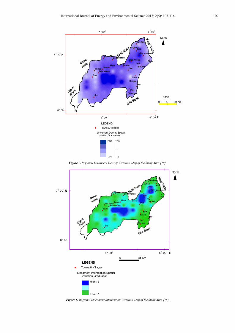
In this extant age of geo-information technology, it is

almost becoming the norm to combine remote sensing and

geophysics in most environmental, groundwater and

engineering site investigation [15-16]. The lineament density

and interception maps “Figures 7 and 8” show a low spatial

variation as the lineaments are generally sparse in the study

area especially in Ose local government area; while Owo

area shows low – moderate variation.

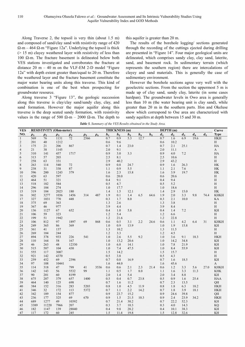
“Tables 5 – 6” give a summary of the results of the VES

curves obtained from the study area. The number of layers

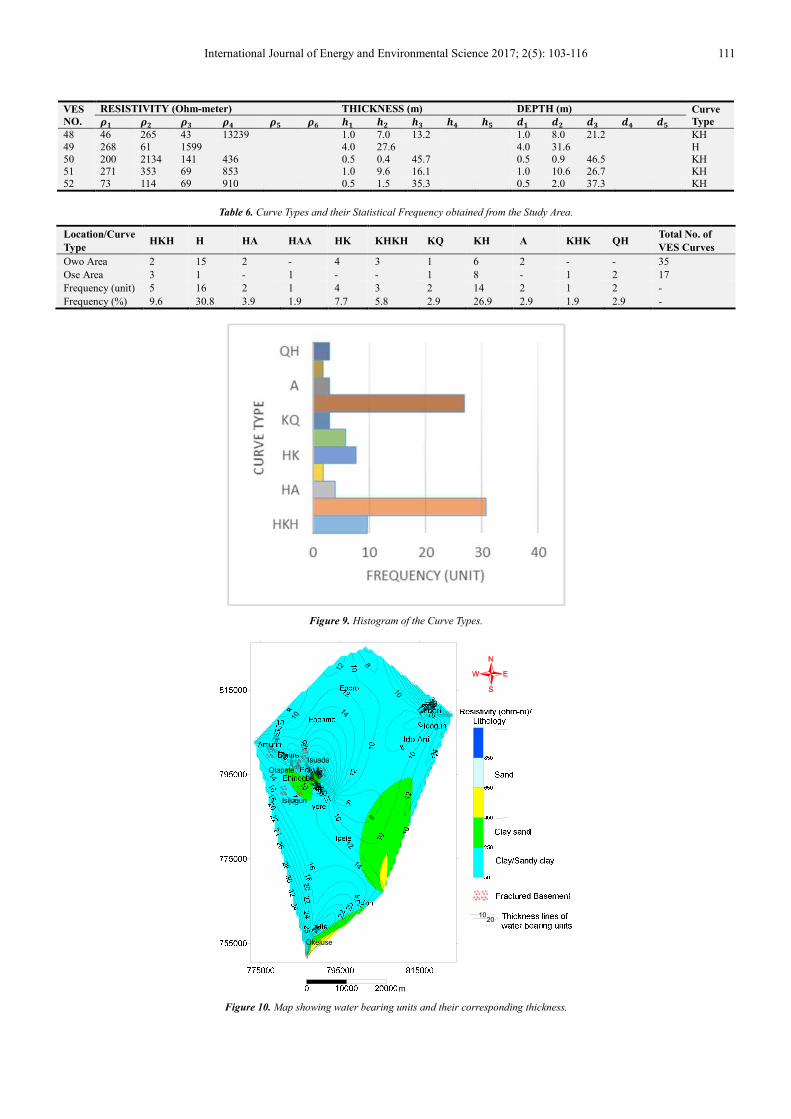
varies between three (3) layers and six (6) layers. Ten curve

types have been identified: HKH, H, HA, HK, KHKH, KQ,

KH, A, KHK, and QH “Figure 9”. The most occurring

curve types identified are H and KH with % frequency of

30 and 26.9. The root mean square (RMS) error of the

generated curve types ranges between 1.8 and 6.1; this

shows models of well smoothened, iterated curves [17]. The

major water bearing units are confined/unconfined fracture

basement and weathered layer. They have thickness that

varies between 2.6 m and 64.6 m. The depth to these water

bearing geological formation is between 1.2 m and 15.9 m

“Figure 10”. The major water bearing formations in the

study area are clay/sandy clay and clay sand. Sand aquifers

are found in the southern areas of the study area with

thickness generally above 20 m. However, the fracture

basement aquifer is widespread in Owo area with thickness

that could be up to 30 m.

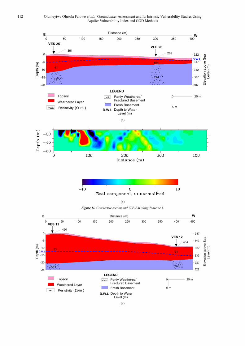
Along Traverse 1, the geoelectric section “Figure 11a”

delineates four geologic layers comprising the topsoil,

weathered layer, fracture basement which is confined within

the fresh basement. The topsoil along this traverse is

composed of clay sand and sandy clay with resistivity in the

range of 100 Ω-m – 300 Ω-m, while clay/sandy clay

underlying it as the weathered material. Fracture zones which

is also identified on the VLF-EM 2-D model as strong

conductive target, suspected to be a water filled geological

formation. The weathered layer is generally very thick (>5

m) especially at eastern flang, but its resistivity values

suggest a clay/clay sand formation. However the major

aquifer along this traverse is the fractured basement. The

flow direction is east – west.


Figure 7. Regional Lineament Density Variation Map of the Study Area [18].

Figure 8. Regional Lineament Interception Variation Map of the Study Area [18).

Okeluse

Ute

Oba Akoko

Sanusi

Ipele

Emure

Ogbagi

Ido Ani

Afo

Okpe

5 00 6 00 E

5 00 6 00

7 30

6 30

I

I

I I

I Io

o

o

o

o o

N

Towns & Villages

Lineament Density Spatial Variation Graduation

Low

High

1

16

170 34 Km

Scale

LEGEND

North

Okeluse

Ute

Oba

Ido AniEmure

Ipele

Afo

Ogbagi

Okpe

Auga

Sanusi

7 30IoN

6 30Io

5 00Io 6 00

IoE

North

0 34 Km

Towns & Villages

Lineament Interception Spatial Variation Graduation

LEGEND

Low : 1

High : 5



Along Traverse 2, the topsoil is very thin (about 1.5 m)

and composed of sand/clay sand with resistivity range of 420

Ω-m – 464 Ω-m “Figure 12a”. Underlying the topsoil is thick

(> 15 m) clayey weathered layer with resistivity of less than

100 Ω-m. The fracture basement is delineated below both

VES stations investigated and corroborates the fracture at

distance 20 m – 40 m on the VLF-EM 2-D model “Figure

12a” with depth extent greater than/equal to 20 m. Therefore

the weathered layer and the fracture basement constitute the

major water bearing units along this traverse. This kind of

combination is one of the best when prospecting for

groundwater resource.

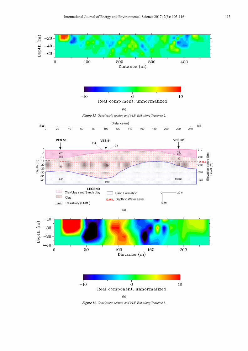
Along traverse 3 “Figure 13”, the geologic succession

along this traverse is clay/clay sand/sandy clay, clay, and

sand formation. However the major aquifer along this

traverse is the deep seated sandy formation, with resistivity

values in the range of 500 Ω-m – 2000 Ω-m. The depth to

this aquifer is greater than 20 m.

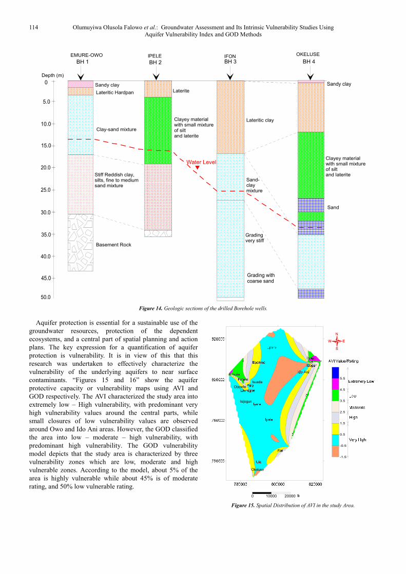
The results of the borehole logging/ sections generated

through the recording of the cuttings ejected during drilling

are presented in “Figure 14”. Four major geological units are

delineated, which comprises sandy clay, clay sand, laterite,

sand, and basement rock. In sedimentary terrain (which

represents the southern region) there are intercalations of

clayey and sand materials. This is generally the case of

sedimentary environment.

However the borehole sections agree very well with the

geoelectric sections. From the section the uppermost 5 m is

made up of clay sand, sandy clay, laterite (in some cases

hardpan). The groundwater levels in Owo area is generally

less than 10 m (the water bearing unit is clay sand), while

greater than 20 m in the southern parts. Ifon and Okeluse

show which correspond to Ose area are characterized with

sandy aquifers at depth between 15 and 30 m.

Table 5. Summary of the VES Results obtained in the Study Area.

VES

NO.

RESISTIVITY (Ohm-meter) THICKNESS (m) DEPTH (m) Curve

Type

1 569 76 1131 72 2566 0.7 0.9 5.3 12.7 0.7 1.6 6.9 19.6 HKH

2 201 40 1212 0.6 9.6 0.6 10.2 H

3 175 21 206 867 0.7 1.4 23.0 0.7 2.1 25.1 HA 4 21 38 1145 2.0 9.1 2.0 11.1 A

5 310 141 457 1717 0.9 3.0 3.3 0.9 4.0 7.2 HA

6 313 57 203 2.5 8.1 2.5 10.6 H 7 258 63 331 2.9 40.2 2.9 43.2 H

8 263 114 540 72 0.9 0.8 24.7 0.9 1.6 26.3 HK

9 238 31 338 87 1.1 0.9 5.5 1.1 2.1 7.6 HK 10 596 200 1243 379 1.6 2.3 15.8 1.6 3.9 19.7 HK

11 420 63 597 0.6 20.0 0.6 20.6 H 12 464 51 321 0.4 9.1 0.4 9.4 H

13 518 182 584 0.5 4.7 0.5 5.2 H

14 296 104 274 1.0 17.7 1.0 18.6 H 15 319 104 2023 180 1.4 1.5 12.1 1.4 2.9 15.0 HK

16 302 3277 1036 1456 314 487 1.9 0.1 1.4 6.5 64.6 1.9 2.0 3.3 9.8 74.4 KHKH

17 327 1031 770 448 0.3 1.7 8.0 0.3 2.1 10.0 KA 18 375 69 363 1.3 2.6 1.3 3.8 H

19 367 46 977 3.9 4.4 3.9 8.4 H

20 136 1127 67 652 0.4 1.0 5.8 0.4 1.4 7.2 KH 21 106 59 323 1.2 5.4 1.2 6.6 H

22 199 51 1942 1.2 21.6 1.2 22.8 H

23 106 812 97 1897 69 868 0.6 0.5 3.1 2.2 24.6 0.6 1.1 4.2 6.4 31 KHKH 24 249 365 86 369 1.0 0.9 13.9 1.0 1.9 15.8 KH

25 361 41 137 1.3 10.2 1.3 11.5 H

26 269 104 244 1.2 3.3 1.2 4.5 H 27 894 378 933 226 541 1.0 2.6 5.5 9.2 1.0 3.6 9.1 18.3 HKH

28 110 164 58 167 1.0 13.2 20.6 1.0 14.2 34.8 KH

29 46 263 48 12330 1.0 6.8 14.1 1.0 7.8 21.9 KH 30 515 587 104 430 1.0 7.4 47.5 1.0 8.4 55.9 KH

31 555 117 3087 1.5 14.2 1.5 15.7 H

32 921 142 4370 0.5 3.8 0.5 4.3 H 33 259 452 69 2396 0.7 0.8 16.9 0.7 1.6 18.5 KH

34 97 108 10441 1.6 44.0 1.6 45.6 A

35 114 318 47 799 41 3536 0.6 0.6 2.1 2.3 21.4 0.6 1.2 3.3 5.6 27.0 KHKH 36 142 143 56 5532 99 1.1 0.5 1.7 8.0 1.1 1.6 3.3 11.3 KHK

37 90 201 60 8199 2.0 1.4 5.4 2.0 3.4 8.8 KH

38 675 207 379 657 1400 0.5 0.4 0.7 23.8 0.5 0.9 1.6 25.4 HAA 39 464 140 125 698 0.7 1.6 11.2 0.7 2.3 13.5 QH

40 384 152 316 283 5203 0.8 1.0 4.5 11.9 0.8 1.8 6.3 18.2 HKH

41 346 32 172 113 5372 0.7 1.1 2.2 14.2 0.7 1.8 3.9 18.1 HKH 42 342 189 154 877 0.9 23.7 15.2 0.9 24.6 39.8 QH

43 236 177 325 69 670 0.9 1.5 21.5 10.3 0.9 2.4 23.9 34.2 HKH

44 689 1277 49 10392 0.7 21.4 30.2 0.7 22.2 52.3 KH 45 3389 11220 7966 207 0.3 3.7 10.3 0.3 4.0 14.3 KQ

46 182 1147 139 28840 0.4 9.8 28.2 0.4 10.1 38.3 KH

47 117 172 60 245 1.5 11.4 19.8 1.5 12.8 32.6 KH


VES

NO.

RESISTIVITY (Ohm-meter) THICKNESS (m) DEPTH (m) Curve

Type

48 46 265 43 13239 1.0 7.0 13.2 1.0 8.0 21.2 KH

49 268 61 1599 4.0 27.6 4.0 31.6 H

50 200 2134 141 436 0.5 0.4 45.7 0.5 0.9 46.5 KH 51 271 353 69 853 1.0 9.6 16.1 1.0 10.6 26.7 KH

52 73 114 69 910 0.5 1.5 35.3 0.5 2.0 37.3 KH

Table 6. Curve Types and their Statistical Frequency obtained from the Study Area.

Location/Curve

Type HKH H HA HAA HK KHKH KQ KH A KHK QH

Total No. of

VES Curves

Owo Area 2 15 2 - 4 3 1 6 2 - - 35

Ose Area 3 1 - 1 - - 1 8 - 1 2 17

Frequency (unit) 5 16 2 1 4 3 2 14 2 1 2 -

Frequency (%) 9.6 30.8 3.9 1.9 7.7 5.8 2.9 26.9 2.9 1.9 2.9 -

Figure 9. Histogram of the Curve Types.

Figure 10. Map showing water bearing units and their corresponding thickness.

1020



(a)

(b)

Figure 11. Geoelectric section and VLF-EM along Traverse 1.

(a)

0 50 100 150 200 250 300 350 400

-20

-15

-10

-5

0

De

pth

(m

)

Ele

va

tion

abo

ve S

ea

Leve

l (m

)

322

317

312

307

302

361

41

137

269

104

244

VES 25VES 26

Distance (m)E W

Topsoil

Weathered Layer

Partly Weathered/Fractured Basement

Fresh Basement

0

5 m

25 m

Resistivity780 ( -m )

LEGEND

D.W.L

D.W.L Depth to Water Level (m)

0 50 100 150 200 250 300 350 400 450

-25

-20

-15

-10

-5

0

De

pth

(m

)

Ele

va

tio

n a

bo

ve

Se

a

L

eve

l (m

)

420

63

597

464

51

321

Distance (m)E W

VES 11

VES 12

Topsoil

Weathered Layer

Partly Weathered/Fractured Basement

Fresh Basement

0

5 m

25 m


LEGEND

347

342

337

332

327

322

D.W.L

D.W.L Depth to Water Level (m)


(b)


(a)

(b)


0 20 40 60 80 100 120 140 160 180 200 220 240

-40

-35

-30

-25

-20

-15

-10

-5

0

De

pth

(m

)

Ele

va

tio

n a

bo

ve

Se

a

Le

ve

l (m

)

Distance (m)

270

260

250

240

230

VES 52VES 50 VES 51

SW NE

46

43

265

13239

271

353

69

853

73114

69

910

Clay/clay sand/Sandy clay

Clay

Sand Formation 0

10 m

20 m


LEGEND

D.W.L

D.W.L Depth to Water Level



Figure 14. Geologic sections of the drilled Borehole wells.

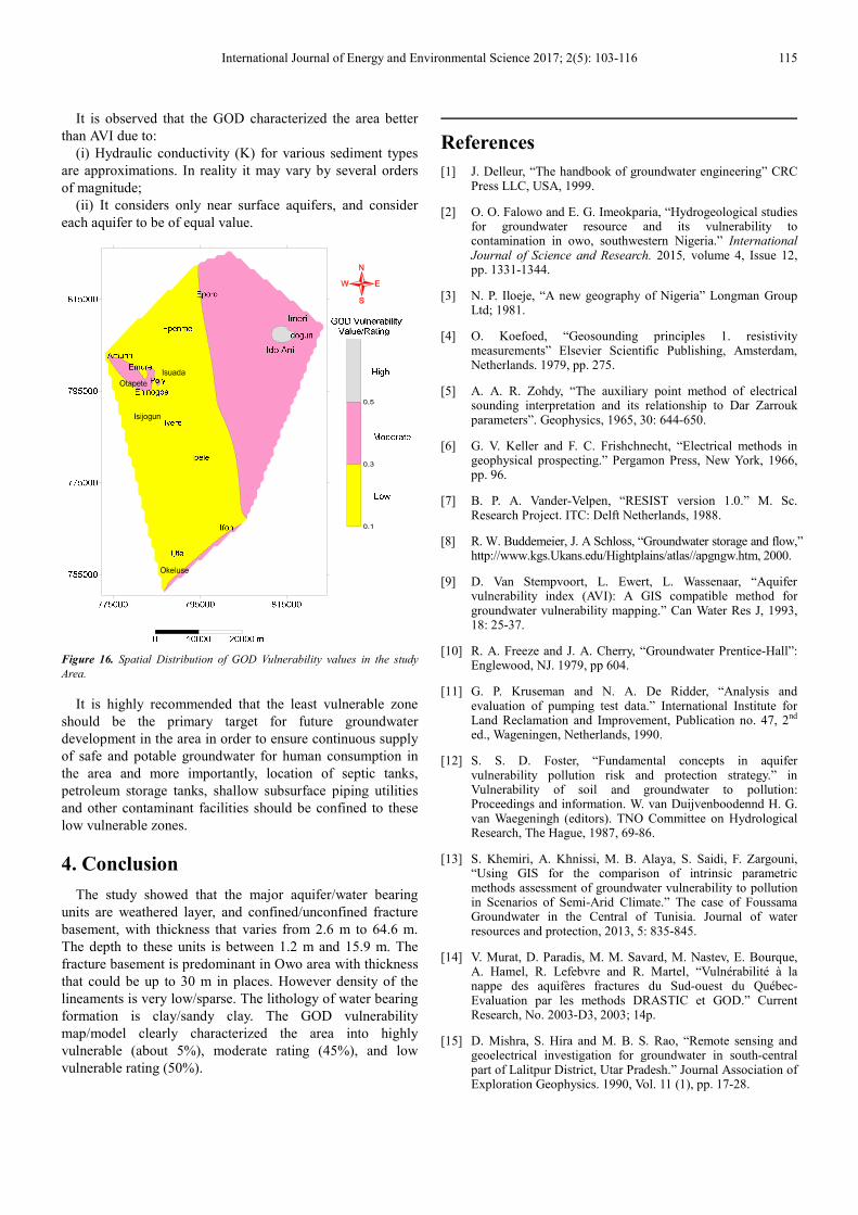
Aquifer protection is essential for a sustainable use of the

groundwater resources, protection of the dependent

ecosystems, and a central part of spatial planning and action

plans. The key expression for a quantification of aquifer

protection is vulnerability. It is in view of this that this

research was undertaken to effectively characterize the

vulnerability of the underlying aquifers to near surface

contaminants. “Figures 15 and 16” show the aquifer

protective capacity or vulnerability maps using AVI and

GOD respectively. The AVI characterized the study area into

extremely low – High vulnerability, with predominant very

high vulnerability values around the central parts, while

small closures of low vulnerability values are observed

around Owo and Ido Ani areas. However, the GOD classified

the area into low – moderate – high vulnerability, with

predominant high vulnerability. The GOD vulnerability

model depicts that the study area is characterized by three

vulnerability zones which are low, moderate and high

vulnerable zones. According to the model, about 5% of the

area is highly vulnerable while about 45% is of moderate

rating, and 50% low vulnerable rating.

Figure 15. Spatial Distribution of AVI in the study Area.

0

5.0

10.0

15.0

20.0

25.0

30.0

35.0

40.0

45.0

50.0

BH 1 BH 2 BH 3 BH 4

EMURE-OWO IPELE IFON OKELUSE

Sandy clay

Lateritic Hardpan

Clay-sand mixture

Basement Rock

Stiff Reddish clay,silts, fine to mediumsand mixture

Laterite

Clayey materialwith small mixtureof siltand laterite

Lateritic clay

Sand-clay mixture

Gradingvery stiff

Grading withcoarse sand

Sandy clay

Clayey materialwith small mixtureof siltand laterite

Sand

Water Level

Depth (m)


It is observed that the GOD characterized the area better

than AVI due to:

(i) Hydraulic conductivity (K) for various sediment types

are approximations. In reality it may vary by several orders

of magnitude;

(ii) It considers only near surface aquifers, and consider

each aquifer to be of equal value.

Figure 16. Spatial Distribution of GOD Vulnerability values in the study

Area.

It is highly recommended that the least vulnerable zone

should be the primary target for future groundwater

development in the area in order to ensure continuous supply

of safe and potable groundwater for human consumption in

the area and more importantly, location of septic tanks,

petroleum storage tanks, shallow subsurface piping utilities

and other contaminant facilities should be confined to these

low vulnerable zones.

4. Conclusion

The study showed that the major aquifer/water bearing

units are weathered layer, and confined/unconfined fracture

basement, with thickness that varies from 2.6 m to 64.6 m.

The depth to these units is between 1.2 m and 15.9 m. The

fracture basement is predominant in Owo area with thickness

that could be up to 30 m in places. However density of the

lineaments is very low/sparse. The lithology of water bearing

formation is clay/sandy clay. The GOD vulnerability

map/model clearly characterized the area into highly

vulnerable (about 5%), moderate rating (45%), and low

vulnerable rating (50%).

References

[1] J. Delleur, “The handbook of groundwater engineering” CRC Press LLC, USA, 1999.

[2] O. O. Falowo and E. G. Imeokparia, “Hydrogeological studies for groundwater resource and its vulnerability to contamination in owo, southwestern Nigeria.” International Journal of Science and Research. 2015, volume 4, Issue 12, pp. 1331-1344.

[3] N. P. Iloeje, “A new geography of Nigeria” Longman Group Ltd; 1981.

[4] O. Koefoed, “Geosounding principles 1. resistivity measurements” Elsevier Scientific Publishing, Amsterdam, Netherlands. 1979, pp. 275.

[5] A. A. R. Zohdy, “The auxiliary point method of electrical sounding interpretation and its relationship to Dar Zarrouk parameters”. Geophysics, 1965, 30: 644-650.

[6] G. V. Keller and F. C. Frishchnecht, “Electrical methods in geophysical prospecting.” Pergamon Press, New York, 1966, pp. 96.

[7] B. P. A. Vander-Velpen, “RESIST version 1.0.” M. Sc. Research Project. ITC: Delft Netherlands, 1988.

[8] R. W. Buddemeier, J. A Schloss, “Groundwater storage and flow,” http://www.kgs.Ukans.edu/Hightplains/atlas//apgngw.htm, 2000.

[9] D. Van Stempvoort, L. Ewert, L. Wassenaar, “Aquifer vulnerability index (AVI): A GIS compatible method for groundwater vulnerability mapping.” Can Water Res J, 1993, 18: 25-37.

[10] R. A. Freeze and J. A. Cherry, “Groundwater Prentice-Hall”: Englewood, NJ. 1979, pp 604.

[11] G. P. Kruseman and N. A. De Ridder, “Analysis and evaluation of pumping test data.” International Institute for Land Reclamation and Improvement, Publication no. 47, 2nd ed., Wageningen, Netherlands, 1990.

[12] S. S. D. Foster, “Fundamental concepts in aquifer vulnerability pollution risk and protection strategy.” in Vulnerability of soil and groundwater to pollution: Proceedings and information. W. van Duijvenboodennd H. G. van Waegeningh (editors). TNO Committee on Hydrological Research, The Hague, 1987, 69-86.

[13] S. Khemiri, A. Khnissi, M. B. Alaya, S. Saidi, F. Zargouni, “Using GIS for the comparison of intrinsic parametric methods assessment of groundwater vulnerability to pollution in Scenarios of Semi-Arid Climate.” The case of Foussama Groundwater in the Central of Tunisia. Journal of water resources and protection, 2013, 5: 835-845.

[14] V. Murat, D. Paradis, M. M. Savard, M. Nastev, E. Bourque, A. Hamel, R. Lefebvre and R. Martel, “Vulnérabilité à la nappe des aquifères fractures du Sud-ouest du Québec- Evaluation par les methods DRASTIC et GOD.” Current Research, No. 2003-D3, 2003; 14p.

[15] D. Mishra, S. Hira and M. B. S. Rao, “Remote sensing and geoelectrical investigation for groundwater in south-central part of Lalitpur District, Utar Pradesh.” Journal Association of Exploration Geophysics. 1990, Vol. 11 (1), pp. 17-28.



[16] A. E. Bala, O. Batelaan and de Smedt “Using Landsat 5 imagery in the assessment of groundwater resources in the crystalline rocks around Dutsin-Ma, northwestern Nigeria.” Journal of Mining and Geology. 2000, Vol. 36 (1), pp. 85-92.

[17] W. H. Barker, “Multispectral scanner. In: Janssen, L. L. F. and Huurneman, G. C. (eds), Principles of remote sensing, ITC Educational Textbook Series, 2001, pp. 71-82.

[18] K. A Mogaji, O. S. Aboyeji, and G. O. Omosuyi, “Mapping of lineaments for groundwater targeting in the basement complex region of Ondo State, Nigeria, using remote sensing and geographic information system (GIS) techniques.” International Journal of Water Resources and Environmental Engineering, 2011, Vol. 3 (7), pp. 150-160.

Groundwater Assessment and Its Intrinsic...

Documents

Transcript of Groundwater Assessment and Its Intrinsic...