Work supported in part by the US Department of Energy contract DE-AC02-76SF00515

SISSA-62/2006/EP

PUPT-2212

SLAC-PUB-12130

Gauge/gravity duality and meta-stable

dynamical supersymmetry breaking

Riccardo Argurio1, Matteo Bertolini2, Sebastian Franco3 and Shamit Kachru4,5

1Physique Theorique et Mathematique and International Solvay Institutes

Universite Libre de Bruxelles, C.P. 231, 1050 Bruxelles, Belgium

2SISSA/ISAS and INFN - Sezione di Trieste

Via Beirut 2; I 34014 Trieste, Italy

3Joseph Henry Laboratories, Princeton University

Princeton, NJ 08544, USA

4Department of Physics and SLAC, Stanford University

Stanford, CA 94305 USA

5Kavli Institute for Theoretical Physics, University of California

Santa Barbara, CA 93106 USA

rargurio@ulb.ac.be, bertmat@sissa.it, sfranco@feynman.princeton.edu,

skachru@stanford.edu

Abstract: We engineer a class of quiver gauge theories with several interesting features

by studying D-branes at a simple Calabi-Yau singularity. At weak ’t Hooft coupling we

argue using field theory techniques that these theories admit both supersymmetric vacua

and meta-stable non-supersymmetric vacua, though the arguments indicating the existence

of the supersymmetry breaking states are not decisive. At strong ’t Hooft coupling we find

simple candidate gravity dual descriptions for both sets of vacua.

hep-th/0610212

Submitted to Journal of High Energy Physics (JHEP)

Contents

1. Introduction 1

2. The theory 4

2.1 Masses from quantum moduli spaces 4

2.2 A ZZ2 orbifold of the conifold 7

2.3 Fractional branes 9

3. The duality cascade 10

3.1 The last cascade step 13

4. The meta-stable non-supersymmetric vacuum 15

4.1 Meta-stable vacuum in Nf = Nc SQCD 16

4.2 Meta-stable vacuum in the ZZ2 orbifold of the conifold 19

5. Gravity dual 21

5.1 Effective superpotential and basic properties of the geometry 21

5.2 Supersymmetric vacua 25

5.3 Non-supersymmetric vacuum 26

5.4 Comments on the full solution 28

6. Conclusions 29

A. Geometry of the moduli space 32

B. Toric geometry, (p, q) webs and complex deformations 35

C. Type IIA description 38

1. Introduction

Quantum field theories which exhibit dynamical breaking of supersymmetry (DSB) may

be relevant in the description of Nature at the electroweak scale [1]. While theories which

1

accomplish DSB were found already in the early 1980s by Affleck, Dine and Seiberg (for a

review of early work, see [2]), the subject has retained much of its interest over the past

25 years. For instance, in the earliest examples, the supersymmetry breaking vacua were

global minima in chiral gauge theories. However, it was realized that by relaxing both

of these criteria, one might obtain simpler examples [3] which could yield less contrived

realistic models of gauge mediation [4]. This insight was further developed in many papers

[5], with perhaps the simplest idea that can yield complete models appearing very recently

in [6]. Meta-stable supersymmetry breaking has also played a crucial role in many recent

constructions of string vacua [7, 8], which quite plausibly realize the idea of a “discretuum”

proposed in [9].

In the past decade, two new tools – Seiberg duality [10] and gauge/gravity duality [11]

– have significantly improved our ability to analyze the dynamics of strongly coupled super-

symmetric gauge theories. Since DSB is a strong-coupling phenomenon in many instances,

these new tools should be exploited to improve our understanding of theories that exhibit

DSB.

Gauge/gravity duality has already been applied in several different examples to illumi-

nate the physics of supersymmetry breaking [12, 13, 14, 15, 16]. In one of these instances, the

3d gauge theory analyzed in [12], the direct field theory analysis [17], and the gravity analysis

were seen to agree. In some other examples, such as those investigated in [14, 15, 16], the

dual gauge theory does not admit any stable vacuum [15, 18, 19]. This is quite plausibly true

in the large ’t Hooft coupling gravity dual as well, though compactifications of the scenario

may fix this problem [20], through the generation of baryonic couplings which were shown to

lead to stable non-supersymmetric vacua in some cases [21]. In [22], it was shown that these

theories exhibit meta-stable non-supersymmetric vacua when massive flavors are added by

means of D7-branes.

The examples of [13] (KPV) will be more relevant to our story. That work builds directly

on the beautiful paper of Klebanov and Strassler [23], where a smooth gravity dual was found

for the cascading SU(N + M)×SU(N) gauge theory of branes and fractional branes at the

conifold. At the end of the cascade (for N a multiple of M) one finds a deformed conifold

geometry with a large sphere of radius√

gsM , and M units of RR three-form flux piercing

the sphere. It was proposed in [13] that by adding p ≪ M anti-D3 brane probes to this

system, one could obtain non-supersymmetric states in the SU(N + M − p) × SU(N − p)

supersymmetric gauge theory realized by branes at the conifold. Because the anti-D3 branes

are attracted to the warped tip of the geometry, the supersymmetry breaking states have

exponentially small vacuum energy. In addition, they are connected by finite energy bubbles

2

of false vacuum decay, to the supersymmetric vacua of the SU(N + M − p) × SU(N − p)

theory [13]. This, together with the fact that the boundary conditions at infinity in the

gravity dual are the same for the supersymmetric and non-supersymmetric states (in contrast

to the situation described in [24]), indicates that these are best thought of as dynamical

supersymmetry breaking states in the SU(N +M − p)×SU(N − p) gauge theory at large ’t

Hooft coupling. These states have played an important role in the KKLT construction [8],

and in some models of inflation in string theory [25, 26]. More importantly for our purpose,

it is obvious that the same analysis would yield meta-stable KPV-like states in many other

confining gauge theories with smooth gravity duals.

In an a priori un-related development, it was recently found in the elegant paper of

Intriligator, Seiberg and Shih [27] (ISS) that even the simplest non-chiral gauge theories

can exhibit meta-stable vacua with DSB. A straightforward application of Seiberg duality to

supersymmetric SU(Nc) QCD with Nf slightly massive quark flavors of mass m ≪ ΛQCD,

in the range Nc ≤ Nf < 32Nc, yields a dual magnetic theory which breaks supersymmetry

at tree-level. The supersymmetry breaking vacuum is a miracle from the perspective of the

electric description, occurring in the strong-coupling regime of small field VEVs where only

the Seiberg dual description allows one to analyze the dynamics. And again, as will be

important for us, the analysis of the original paper can be extended to provide many other

examples.1

On closer inspection, there are several qualitative similarities between the KPV states

(which were found using gauge/gravity duality) and the ISS states (which were found using

Seiberg duality). In both examples, the supersymmetry breaking state is related to the

existence of a baryonic branch; in both examples, it is a meta-stable state in a non-chiral

gauge theory; and in both examples, there is an intricate moduli space of Goldstone modes

(geometrized in the KPV case as the translation modes of the anti-D3s at the end of the

Klebanov-Strassler throat). It is natural to wonder – is there some direct relation between

these two classes of meta-stable states?2

In this paper, we propose that at least in some cases, the answer is yes . We analyze the

gauge theory on D-branes at a certain simple singularity (obtained from a ZZ2 quotient of

the conifold). We find that this non-chiral gauge theory admits both supersymmetric and

supersymmetry breaking vacua – the non-supersymmetric vacua being found by a simple

generalization of ISS. At large ’t Hooft coupling, our system has a simple dual gravitational

1Some references which are in some respect relevant to our work are [28, 29, 30, 31].2This question has been raised by the present authors, H. Ooguri, N. Seiberg, H. Verlinde and many

others.

3

description, along the lines of [23]. We analyze the dual geometry, and propose natural

candidates for the gravity description of both sets of vacua – with the non-supersymmetric

vacua arising from a simple generalization of KPV. Our result suggests that there may be a

general connection between the classes of states that are unveiled using the two techniques.

Of course, this is example dependent: there is no firm argument that meta-stable states

which are present at large ’t Hooft coupling continue smoothly back to weak gauge coupling,

or vice versa, in general. For this reason, it is not clear that the states of the original ISS

model should have a simple gravity dual (or, that the states of the original KPV model,

should have a simple weak-coupling description).

The organization of our paper is as follows. In §2, we describe the gauge theory that we

will analyze, and a possible brane configuration in string theory that gives rise to it. In §3,

we will describe a duality cascade (similar to the one in [23]) which will serve as a possible

field theory UV-completion of our model; the gauge theory we will focus on arises at the

end of the cascade. In §4, we argue, using field theory techniques, that our gauge theory

admits meta-stable states that dynamically break supersymmetry, in addition to various

supersymmetric vacua. In §5, we provide a description of candidate gravity duals for both

the supersymmetric and supersymmetry breaking vacua. We conclude with a discussion

of possible directions for further research and open questions in §6. We have relegated a

detailed discussion of the geometry of the moduli space, complex deformations from toric

geometry and a (T-dual) IIA brane system, to several appendices.

2. The theory

In this section we present our model. We first present a prototype model that has some of

the properties we are interested in finding. More precisely, this model exhibits ISS-like meta-

stable vacua in a gauge theory where the very small flavor masses are not put in by hand,

but instead are generated dynamically. Then, in order to illustrate our ideas, we provide a

concrete and simple D-brane/string background which will serve as our privileged toy model

in the rest of the paper. It should be kept in mind, however, that our proposal has a wide

range of applicability and in principle many different string constructions could lead to this

kind of dynamics.

2.1 Masses from quantum moduli spaces

A key ingredient in the construction of ISS-like models with non-supersymmetric meta-

stable vacua is the existence of massive flavors. Since we do not want to introduce external

4

masses, the only remaining option is to generate them dynamically by giving VEVs to fields

participating in a cubic (or higher) vertex in the superpotential. Moreover, if we want to

forbid those VEVs from relaxing to zero (which they may wish to do dynamically, since

the vacuum energy of the would-be non-supersymmetric vacua is proportional to the quark

masses), we have to impose at least one constraint on them. The most natural such constraint

is the one describing the quantum deformed moduli space of Nf = Nc SQCD [32].3 Hence,

we are naturally led to a model of a quiver gauge theory which features at least one node in

this regime.

Before presenting all the details in later sections, we briefly review here the simple

mechanism that we want to propose in order to generate such masses dynamically. Let us

consider the quiver diagram shown in Figure 1 with a tree level superpotential involving at

least the quartic interaction

W = . . . + X21X12X23X32 + . . . (2.1)

where here and henceforth, traces on gauge indices are understood.

Let us remind the reader that a quiver diagram is just a convenient pictorial way to

encode the matter content of certain gauge theories. Every node in the quiver represents a

gauge group (in this paper we will focus on SU(Ni) gauge groups). An arrow connecting

two nodes represents a chiral multiplet transforming in the fundamental representation of

the node at its tail and the anti-fundamental representation of the node at its head.

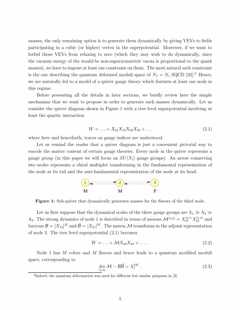
M M P

1 2 3

Figure 1: Sub-quiver that dynamically generates masses for the flavors of the third node.

Let us first suppose that the dynamical scales of the three gauge groups are Λ1 ≫ Λ3 ≫Λ2. The strong dynamics of node 1 is described in terms of mesons Mi2,j2 = X i2,i1

21 X i1,j221 and

baryons B = [X12]M and B = [X21]

M . The meson M transforms in the adjoint representation

of node 2. The tree level superpotential (2.1) becomes

W = . . . + MX23X32 + . . . . (2.2)

Node 1 has M colors and M flavors and hence leads to a quantum modified moduli

space, corresponding to

deti2,j2

M−BB = Λ2M1 . (2.3)

3Indeed, the quantum deformation was used for different but similar purposes in [3].

5

On the mesonic branch, 〈B〉 = 〈B〉 = 0 and deti2,j2〈M〉 = Λ2M1 . The gauge group is

higgsed down to SU(P )×U(1)M−1, with the abelian factors coming from the adjoint higgsing

of the second node.

From the point of view of node 3, X23 and X32 give rise to M flavors with i2 becoming

a flavor index. When the expectation value of M is plugged into (2.2), it gives rise to non-

zero masses for these flavors. The theory becomes precisely SU(P ) SQCD with M massive

flavors. The masses are constrained by (2.3) but are dynamical quantities. In order to follow

the argument of ISS, we would then perform a Seiberg duality on node 3, which is the one

responsible for DSB.

The Λ1 ≫ Λ3 ≫ Λ2 regime we have just discussed is the simplest to study, since as

we lower the energy scale we first generate the masses for the flavors of node 3. However,

in order for the analysis of ISS to be valid, flavor masses should be much smaller than the

dynamical scale Λ3.

Since the masses are dictated by Λ1, it is more natural to achieve a small mass to Λ3

ratio for Λ3 ≫ Λ1 ≫ Λ2. If P < M , we begin by dualizing node 3. If P +1 ≤ M < 32P , node

3 is IR free in the dual theory. In the magnetic theory, there are mesons N i2,j2 = X i2,i323 X i3,j2

32

and “dual quarks” Y32 and Y23. The superpotential becomes

Wmag = . . . + X21X12 N + N Y23Y32 + . . . , (2.4)

where the first terms comes from (2.2) and the second one is the usual cubic coupling between

Seiberg mesons and dual quarks. At the Λ1 scale, node 1 develops a quantum moduli space

as in (2.3). Going to the mesonic branch, the superpotential becomes

Wmag = . . . + 〈M〉 N + N Y23Y32 + . . . . (2.5)

The rank condition of ISS [27] arises from the F-term of N . 4

We thus conclude that our model potentially admits meta-stable nonsupersymmetric

vacua for both Λ1 ≫ Λ3 ≫ Λ2 and Λ3 ≫ Λ1 ≫ Λ2. In fact, we have shown that going on

the quantum deformed mesonic branch of node 1, and performing the Seiberg duality on

node 3, are commuting operations. Hence we do not have to assume an a priori hierarchy

between the scales Λ1 and Λ3. A more detailed examination in §4 will show that the only

really plausible case is when M = P .5 There, it is natural to assume strong dynamics at

4The rank condition corresponds to the inability to have all FN i2,j2 = 0 because the rank of node 3 in

the magnetic theory (which determines the maximum possible rank of Y23Y32) is (M −P ), smaller than the

dimension of N .5The argument for the existence of a meta-stable vacuum when P = M is more subtle, see §4.

6

both nodes 1 and 3 simultaneously. In §5.1 we argue that essentially any hierarchy between

Λ1 and Λ3 is attainable in a string theory realization of this model.

The gauge theory described above can be viewed as a sub-sector embedded in a larger

quiver, with possibly more gauge groups, fields (even charged under node 3) and superpo-

tential interactions.

2.2 A ZZ2 orbifold of the conifold

In this section we present a theory that contains the sub-quiver discussed in §2.1 and hence

has the appropriate non-chiral matter and quartic interactions to generate dynamical masses

by quantum deformation of the moduli space. In addition, this model has a concrete string

theory realization in terms of D-branes probing a singularity.

The model we consider is a non-chiral ZZ2 orbifold of the conifold (see e.g. [33]). It follows

from the conifold gauge theory by the standard orbifolding procedure. Figure 2 shows the

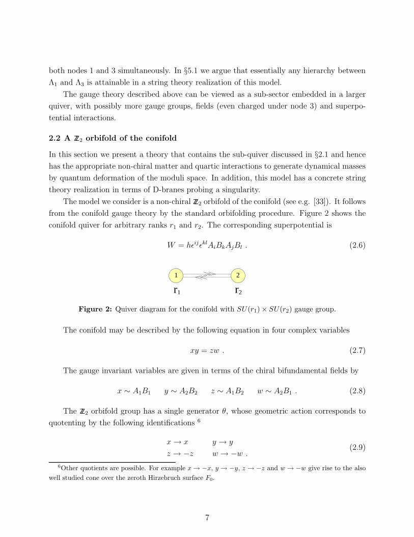
conifold quiver for arbitrary ranks r1 and r2. The corresponding superpotential is

W = hǫijǫklAiBkAjBl . (2.6)

r1 r2

1 2

Figure 2: Quiver diagram for the conifold with SU(r1) × SU(r2) gauge group.

The conifold may be described by the following equation in four complex variables

xy = zw . (2.7)

The gauge invariant variables are given in terms of the chiral bifundamental fields by

x ∼ A1B1 y ∼ A2B2 z ∼ A1B2 w ∼ A2B1 . (2.8)

The ZZ2 orbifold group has a single generator θ, whose geometric action corresponds to

quotenting by the following identifications 6

x → x y → y

z → −z w → −w .(2.9)

6Other quotients are possible. For example x → −x, y → −y, z → −z and w → −w give rise to the also

well studied cone over the zeroth Hirzebruch surface F0.

7

We can define new variables that are invariant under the orbifold group. From the action

in (2.9), they are x′ = x, y′ = y, z′ = z2 and w′ = w2. It is now straightforward to see that

the orbifolded geometry is given by the following equation

x′2y′2 = w′z′ . (2.10)

We re-derive this equation from the field theory in appendix A. The resulting geometry

turns out to be toric. A convenient way to describe toric geometries is via toric diagrams and

(p, q) webs, this being a useful way for visualizing the geometric structure of the singularity,

the possible complex structure deformations, the number (and type) of allowed fractional

branes, etc. Appendix B provides a brief review of toric geometry and the applications of

(p, q) webs together with a more detailed analysis of the case under investigation.

Let us now construct the orbifolded gauge theory. We start from the conifold theory

with SU(r1) × SU(r2) gauge group. The coordinates are related to the chiral fields as in

(2.8). It follows that the geometric action of the orbifold group generator θ given by (2.9)

can be implemented by

A1 → −A1 A2 → A2

B1 → −B1 B2 → B2 .(2.11)

In addition, we have to specify the action of θ on the Chan-Paton factors of the two

gauge groups. We take it to be

γθ,1 = diag(1N1,−1N3

)

γθ,2 = diag(1N2,−1N4

)(2.12)

where N1 + N3 = r1 and N2 + N4 = r2. The resulting gauge group is∏4

i=1 SU(Ni). Both

the conifold gauge theory and the orbifold we are studying are completly non-chiral. Hence

there are no constraints on the ranks of the various gauge groups coming from anomaly

cancellation – they are completely arbitrary. Combining the geometric and Chan-Paton

actions, we conclude that the original fields give rise to the following chiral multiplets

A1 → X14, X32 A2 → X12, X34

B1 → X41, X23 B2 → X21, X43 .(2.13)

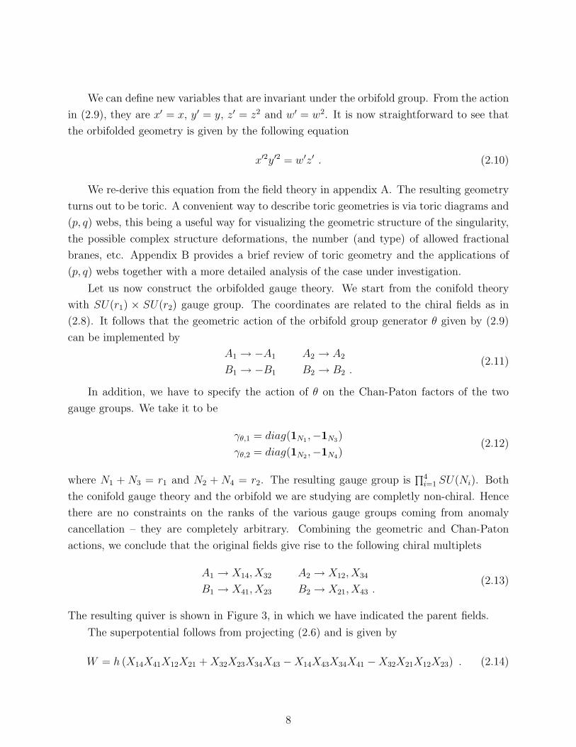
The resulting quiver is shown in Figure 3, in which we have indicated the parent fields.

The superpotential follows from projecting (2.6) and is given by

W = h (X14X41X12X21 + X32X23X34X43 − X14X43X34X41 − X32X21X12X23) . (2.14)

8

B1A1

B2

B1 A1

A2

B2

A2

N1

N3N4

N2

1 2

34

Figure 3: Quiver diagram for the ZZ2 orbifold of the conifold under consideration, for arbitrary

numbers of fractional and regular D3-branes. We have labeled bifundamentals according to the

parent field.

2.3 Fractional branes

This theory has three types of fractional branes. They correspond to different ways in which

D5-branes can be wrapped over 2-cycles collapsed at the tip of the singularity. At the level

of the gauge theory, this corresponds to the already noted fact that anomaly freedom does

not constrain the ranks of the four gauge groups. A convenient basis of fractional branes is

given by the rank vectors (1, 1, 0, 0), (0, 0, 1, 0) and (1, 0, 0, 0). In this language, (1, 1, 1, 1)

represents a regular D3-brane.

In [15], a classification of fractional branes based on the IR behavior they trigger was

introduced. It turns out there are three different classes of fractional branes:

• N = 2 fractional branes: the quiver gauge theory on them (in the absence of regular

D3-branes) has closed oriented loops (gauge invariant operators) that do not appear in the

superpotential. Hence, these fractional branes have flat directions parametrized by the ex-

pectation values of these mesonic operators. From a geometric point of view, these fractional

branes arise when the singularities are not isolated, but have curves of C2/ZZN singularities

passing through them. The IR dynamics of the gauge theories (instantons and Seiberg-

Witten points) map to an enhancon mechanism in a gravity dual description [34].

• Deformation fractional branes: the quiver on these branes is either a set of decoupled nodes,

or nodes with closed loops that appear in the superpotential. The ranks of all gauge factors

are equal. Geometrically, these fractional branes are associated with a possible complex

deformation of the singularity. In the gauge theory, the gauge groups which are involved

9

undergo confinement. This is translated to a complex structure deformation leading to finite

size 3-cycles in the gravity dual.

• DSB fractional branes: these are fractional branes of any other kind, hence they provide the

generic case. In this case, the non-trivial gauge factors have unequal ranks. Geometrically,

they are associated with geometries for which the corresponding complex deformation is

obstructed. The gauge theory dynamics corresponds to the appearance of an Affleck-Dine-

Seiberg (ADS) superpotential [35] that removes the supersymmetric vacuum [14, 15, 16].

Furthermore (as first discussed in [15] and later studied in detail in [18, 19]) the gauge

theory has a runaway behavior towards infinity parametrized by di-baryonic operators.

It is important to keep in mind that combining fractional branes in one or more of

these classes can lead to fractional branes of another kind. In the example under study,

the (0, 0, 1, 0) and (1, 0, 0, 0) branes are deformation fractional branes, while (1, 1, 0, 0) is an

N = 2 fractional brane.

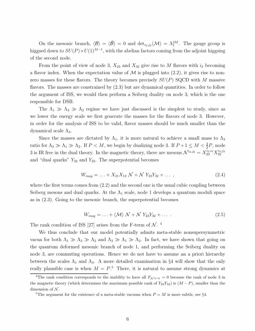
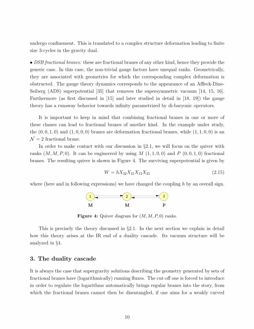
In order to make contact with our discussion in §2.1, we will focus on the quiver with

ranks (M, M, P, 0). It can be engineered by using M (1, 1, 0, 0) and P (0, 0, 1, 0) fractional

branes. The resulting quiver is shown in Figure 4. The surviving superpotential is given by

W = hX32X21X12X23 (2.15)

where (here and in following expressions) we have changed the coupling h by an overall sign.

M M P

1 2 3

Figure 4: Quiver diagram for (M,M,P, 0) ranks.

This is precisely the theory discussed in §2.1. In the next section we explain in detail

how this theory arises at the IR end of a duality cascade. Its vacuum structure will be

analyzed in §4.

3. The duality cascade

It is always the case that supergravity solutions describing the geometry generated by sets of

fractional branes have (logarithmically) running fluxes. The cut-off one is forced to introduce

in order to regulate the logarithms automatically brings regular branes into the story, from

which the fractional branes cannot then be disentangled, if one aims for a weakly curved

10

supergravity description. The same holds for the quiver in Figure 4 which should be thought

of as part of a more general theory, involving regular branes, too.

In general, the dynamics of stacks of fractional and regular branes gets a natural inter-

pretation in terms of a duality cascade (for N = 1 gauge/gravity dualities). This is well

understood for the case of the conifold [36, 23, 37]. However, when departing from this well

known example and focusing on more involved theories, it is not straightforward to visualize

a specific pattern [38, 39]. Here, we will provide one. The discussion is somewhat involved,

and a reader who is interested purely in the dynamics of the quiver in Figure 4 can skip this

section on a first reading.

In general, the physics of a cascade is obtained when one perturbs a fixed point of some

SCFT, generated by N regular D3-branes at a singularity, with some (smaller) number of

fractional D3-branes. This brings the theory out of the fixed point and triggers a non-trivial

RG-flow. What happens, in a quite model-independent way, is that the number of regular

branes effectively diminishes along the flow and the IR dynamics of the theory is determined

by fractional branes only. Therefore, the natural guess for the UV theory generating via

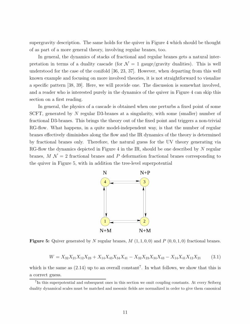
RG-flow the dynamics depicted in Figure 4 in the IR, should be one described by N regular

branes, M N = 2 fractional branes and P deformation fractional branes corresponding to

the quiver in Figure 5, with in addition the tree-level superpotential

N

N+M N+M

N+P

1 2

34

Figure 5: Quiver generated by N regular branes, M (1, 1, 0, 0) and P (0, 0, 1, 0) fractional branes.

W = X32X21X12X23 + X14X43X34X41 − X32X23X34X43 − X14X41X12X21 (3.1)

which is the same as (2.14) up to an overall constant7. In what follows, we show that this is

a correct guess.7In this superpotential and subsequent ones in this section we omit coupling constants. At every Seiberg

duality dynamical scales must be matched and mesonic fields are normalized in order to give them canonical

11

For a cascade to actually occur, the theory should be self-similar, that is after a certain

number of Seiberg dualities it should return to itself (including the superpotential), but with

a reduced number N of regular branes. This model, unlike its cousin the conifold, needs

more than one Seiberg duality to display its self-similar structure. In fact, a possible pattern

is via four subsequent duality steps, where these are taken on the gauge groups of nodes 1, 3,

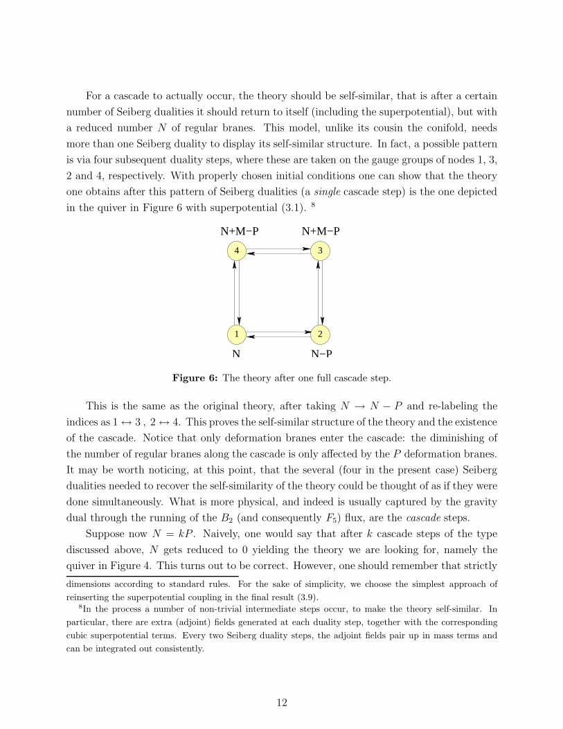
2 and 4, respectively. With properly chosen initial conditions one can show that the theory

one obtains after this pattern of Seiberg dualities (a single cascade step) is the one depicted

in the quiver in Figure 6 with superpotential (3.1). 8

N−P

N+M−P

N

N+M−P

1 2

34

Figure 6: The theory after one full cascade step.

This is the same as the original theory, after taking N → N − P and re-labeling the

indices as 1 ↔ 3 , 2 ↔ 4. This proves the self-similar structure of the theory and the existence

of the cascade. Notice that only deformation branes enter the cascade: the diminishing of

the number of regular branes along the cascade is only affected by the P deformation branes.

It may be worth noticing, at this point, that the several (four in the present case) Seiberg

dualities needed to recover the self-similarity of the theory could be thought of as if they were

done simultaneously. What is more physical, and indeed is usually captured by the gravity

dual through the running of the B2 (and consequently F5) flux, are the cascade steps.

Suppose now N = kP . Naively, one would say that after k cascade steps of the type

discussed above, N gets reduced to 0 yielding the theory we are looking for, namely the

quiver in Figure 4. This turns out to be correct. However, one should remember that strictly

dimensions according to standard rules. For the sake of simplicity, we choose the simplest approach of

reinserting the superpotential coupling in the final result (3.9).8In the process a number of non-trivial intermediate steps occur, to make the theory self-similar. In

particular, there are extra (adjoint) fields generated at each duality step, together with the corresponding

cubic superpotential terms. Every two Seiberg duality steps, the adjoint fields pair up in mass terms and

can be integrated out consistently.

12

speaking the final step of a cascade is not described by a Seiberg duality since generically, at

such energy scales, at least one gauge group ends up having Nf = Nc and the moduli space

is deformed at the quantum level. As in the well-studied case of the conifold, in our case

one can show that the strongly coupled gauge group confines and along the baryonic branch

one indeed ends up with the theory in Figure 4 (while, as in the conifold case, the mesonic

branch has instead P freely-moving regular branes in the background [40]).

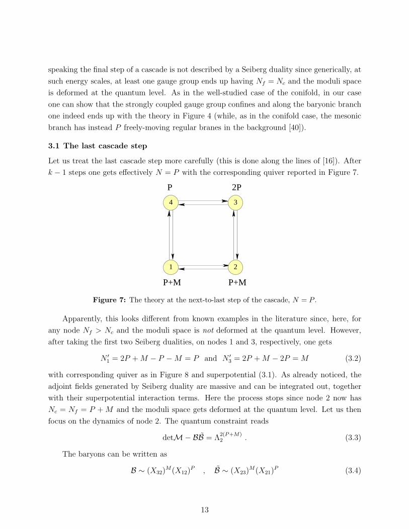
3.1 The last cascade step

Let us treat the last cascade step more carefully (this is done along the lines of [16]). After

k − 1 steps one gets effectively N = P with the corresponding quiver reported in Figure 7.

P 2P

P+MP+M

1 2

34

Figure 7: The theory at the next-to-last step of the cascade, N = P .

Apparently, this looks different from known examples in the literature since, here, for

any node Nf > Nc and the moduli space is not deformed at the quantum level. However,

after taking the first two Seiberg dualities, on nodes 1 and 3, respectively, one gets

N ′1 = 2P + M − P − M = P and N ′

3 = 2P + M − 2P = M (3.2)

with corresponding quiver as in Figure 8 and superpotential (3.1). As already noticed, the

adjoint fields generated by Seiberg duality are massive and can be integrated out, together

with their superpotential interaction terms. Here the process stops since node 2 now has

Nc = Nf = P + M and the moduli space gets deformed at the quantum level. Let us then

focus on the dynamics of node 2. The quantum constraint reads

detM−BB = Λ2(P+M)2 . (3.3)

The baryons can be written as

B ∼ (X32)M(X12)

P , B ∼ (X23)M(X21)

P (3.4)

13

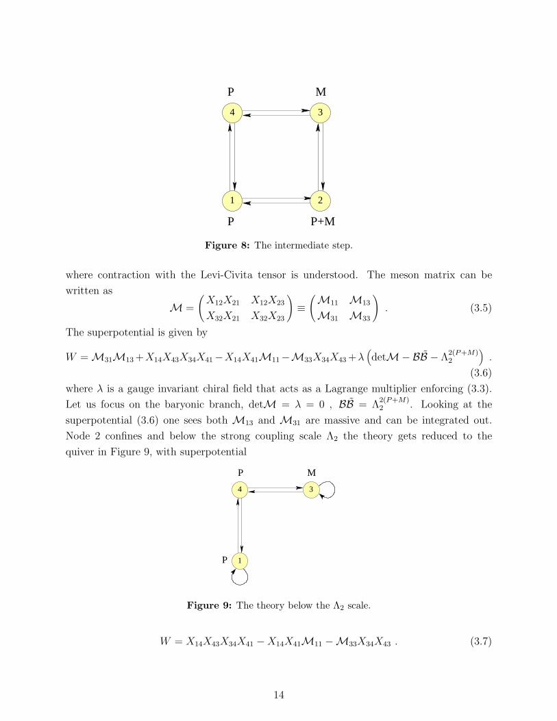
P M

P+MP

1 2

34

Figure 8: The intermediate step.

where contraction with the Levi-Civita tensor is understood. The meson matrix can be

written as

M =

(

X12X21 X12X23

X32X21 X32X23

)

≡(M11 M13

M31 M33

)

. (3.5)

The superpotential is given by

W = M31M13 +X14X43X34X41−X14X41M11−M33X34X43 +λ(

detM−BB − Λ2(P+M)2

)

.

(3.6)

where λ is a gauge invariant chiral field that acts as a Lagrange multiplier enforcing (3.3).

Let us focus on the baryonic branch, detM = λ = 0 , BB = Λ2(P+M)2 . Looking at the

superpotential (3.6) one sees both M13 and M31 are massive and can be integrated out.

Node 2 confines and below the strong coupling scale Λ2 the theory gets reduced to the

quiver in Figure 9, with superpotential

P

P M

1

34

Figure 9: The theory below the Λ2 scale.

W = X14X43X34X41 − X14X41M11 −M33X34X43 . (3.7)

14

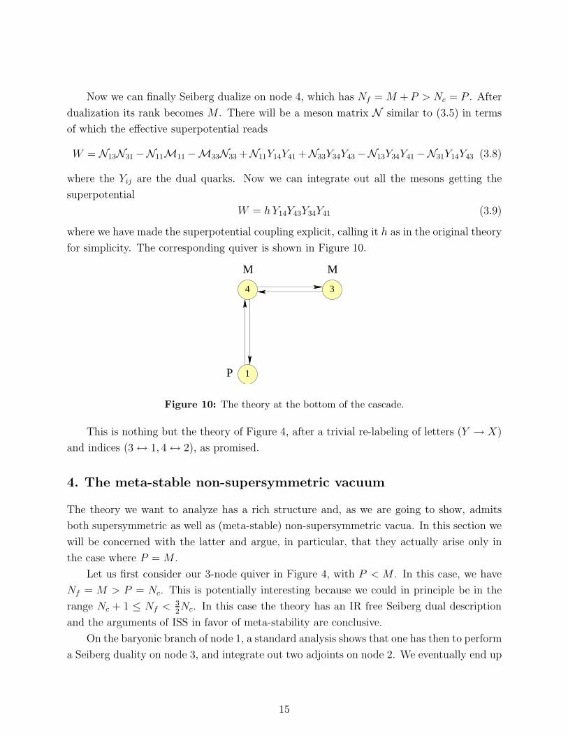
Now we can finally Seiberg dualize on node 4, which has Nf = M + P > Nc = P . After

dualization its rank becomes M . There will be a meson matrix N similar to (3.5) in terms

of which the effective superpotential reads

W = N13N31 −N11M11 −M33N33 +N11Y14Y41 +N33Y34Y43 −N13Y34Y41 −N31Y14Y43 (3.8)

where the Yij are the dual quarks. Now we can integrate out all the mesons getting the

superpotential

W = h Y14Y43Y34Y41 (3.9)

where we have made the superpotential coupling explicit, calling it h as in the original theory

for simplicity. The corresponding quiver is shown in Figure 10.

P

MM

1

34

Figure 10: The theory at the bottom of the cascade.

This is nothing but the theory of Figure 4, after a trivial re-labeling of letters (Y → X)

and indices (3 ↔ 1, 4 ↔ 2), as promised.

4. The meta-stable non-supersymmetric vacuum

The theory we want to analyze has a rich structure and, as we are going to show, admits

both supersymmetric as well as (meta-stable) non-supersymmetric vacua. In this section we

will be concerned with the latter and argue, in particular, that they actually arise only in

the case where P = M .

Let us first consider our 3-node quiver in Figure 4, with P < M . In this case, we have

Nf = M > P = Nc. This is potentially interesting because we could in principle be in the

range Nc + 1 ≤ Nf < 32Nc. In this case the theory has an IR free Seiberg dual description

and the arguments of ISS in favor of meta-stability are conclusive.

On the baryonic branch of node 1, a standard analysis shows that one has then to perform

a Seiberg duality on node 3, and integrate out two adjoints on node 2. We eventually end up

15

in a two node SU(M) × SU(M − P ) quiver with vanishing tree level superpotential. What

was formerly labeled node 2 develops an ADS runaway superpotential and there is no stable

vacuum.

On the mesonic branch of node 1, we have the supersymmetric moduli space of the

N = 2 fractional branes. This is best seen assuming that the VEVs of the mesons M give

a mass to the flavors of node 3, and integrating the latter out. Hence at every point on the

moduli space we have the P vacua of SU(P ) SYM.

As for the non supersymmetric states, following §2.1 and the analysis of [27], we would

expect a meta-stable vacuum with vacuum energy

Vmeta ∼ |Λ3|2P∑

i=1

|hmi|2 (4.1)

where m1, . . . , mP are the P eigenvalues of M with smallest absolute values. Clearly, the

constraint detM = Λ2M1 does not set a minimum value for them. What happens is that

m1, . . . , mP relax to zero, while some of the other eigenvalues run away to infinity so that

detM remains constant. As a result, we conclude that there is no SUSY breaking ISS state

for P < M .

We can also briefly ask what happens in the case P > M . The baryonic branch can be

shown to have a runaway because the SU(P ) node has an ADS superpotential which drives

the meson M to infinity. The supersymmetric mesonic branch is exactly as above. The

ISS-like meta-stable states are absent because Nf < Nc for the SU(P ) gauge group.

We are thus left with only one potentially interesting case, namely P = M . We now show

that there is indeed evidence, albeit weaker, for both supersymmetric and supersymmetry

breaking states in this case.

4.1 Meta-stable vacuum in Nf = Nc SQCD

We begin by reviewing how we can heuristically recover the meta-stable vacua conjectured to

exist by Intriligator, Seiberg and Shih [27] in Nf = Nc SQCD. We note that their conjecture

for this case is based on somewhat weaker evidence than for the cases with Nc + 1 ≤ Nf <32Nc.

Supposing that the quark chiral fields have a small mass m, the low energy effective

superpotential for the mesons M = QQ and the baryons is

W = trm M + λ(detM−BB − Λ2Nc) . (4.2)

The F-term conditions are

detM−BB = Λ2Nc , m + λ(detM)M−1 = 0 , λB = 0 = λB . (4.3)

16

If we are to satisfy the equation involving m, we must have λ 6= 0. This implies that

B = B = 0, which we usually refer to as being on the mesonic branch. Then the constraint

detM = Λ2Nc eventually leads to a SUSY vacuum with mesonic VEVs

M = m−1(det m)1

Nc Λ2 ∼ Λ2 . (4.4)

We assume here and below that the masses are all of the same order. With this assumption,

note that the mass dependence of the mesonic VEVs actually cancels.

Alternatively, if we want to give non zero VEVs to the baryons, B, B 6= 0, which is usually

referred to as being on the baryonic branch, we must set λ = 0. The equation involving m

can no longer be satisfied, and this gives rise to the non-vanishing F-terms contributing to

the vacuum energy. Taking for convenience a mass matrix proportional to the identity, we

would get

Vmeta ∼ Nc|m|2|Λ|2 . (4.5)

The factor of Λ comes from the proper normalization of the meson field M (whose

F-term is non-vanishing), under the assumption that we are at a smooth (though strongly

coupled) point in the moduli space.

Note that though we have referred to mesonic and baryonic branches, they are not

really disconnected.9 The only (Nc) SUSY vacua have fixed non zero VEVs for the mesons

and vanishing VEVs for the baryons. Thus any state with different VEVs on the original

quantum moduli space is a non SUSY state. Clearly most of those states are not meta-stable

(they have tadpoles), and smoothly relax to the SUSY vacua. The argument by ISS, based

on m ≪ Λ and the relation to the more controlled case of Nf = Nc + 1, is that far from the

SUSY states, i.e. when the baryons have the largest allowed VEVs, the state is meta-stable.

It can be shown that the tree-level potential has indeed an extremum there, which remains

flat at second order in the perturbations. We should emphasize again that the Nf = Nc case

is the one in which the ISS arguments favoring the existence of a meta-stable vacuum are

least explicit.

Meta-stability should of course eventually be verified by checking how the pseudo-moduli

are lifted around that vacuum. Relevant considerations about the Kahler potential in a sys-

9We assume here that even on the non SUSY states, the constraint has to be applied. Indeed, the

constraint is in fact a non dynamical F-term, hence it cannot be violated. It is a relation in the chiral

ring which has no classical nor perturbative corrections in any state. The only way it could be evaded is

by non-perturbative D exact contributions which could be non vanishing in a non SUSY state. Though

presumably most of these corrections can be excluded by further considerations, even if they are there, they

will not change significantly the structure of the constraint, just shifting by a small amount the effective

value of Λ2Nc in the non SUSY state.

17

tem very similar to the one discussed here and below can be found in [3], where arguments

in favor of a local minimum are given. It would also be interesting to investigate the tra-

jectories in field space connecting the meta-stable vacuum to the SUSY ones along which

the potential barrier coming from the tree-level superpotential is minimum. The height and

width of the potential barrier determine the lifetime of the meta-stable vacuum.

Here, we make one more comment about the lifting of pseudo-moduli that applies to

compactifications of our solutions (along the lines of [41]). On the baryonic branch, there

is a U(1)B symmetry which is spontaneously broken by the baryon VEV. In the decoupled

theory, this U(1)B is a global symmetry, and its breaking gives rise to a Goldstone boson and

its saxion partner (as discussed in, for instance, [42]). The saxion is a dangerous direction –

its masslessness is not protected by a symmetry, and in any non-supersymmetric vacuum, one

can worry that it could become tachyonic. In compactifications of this kind of theory, there

is one known computable contribution to the mass that acts in the direction of stabilizing

the supersymmetry breaking vacuum.

String compactifications do not have continuous global symmetries. Instead, the U(1)B

becomes a gauge symmetry. The baryon VEVs then give mass to the U(1) gauge boson via

the Higgs mechanism, and the would-be Goldstone multiplet is “eaten.” The relevant mass

that is imparted is proportional to the product of the gauge coupling and the baryon VEVs,

and following §6 of [42], this can be estimated as follows. If the hierarchy of scales generated

by the cascade is ∼ e−τmax , then the mass will be

Msaxion ∼ gs√τmax

Λ . (4.6)

Therefore, as long as one works in a compactification where this mass scale is larger

than the other effects communicating the SUSY-breaking auxiliary field VEV to the saxion

(which is not always true), the Higgs mechanism acts to help remove this possible source

of instability. This remark is relevant to the Goldstone/saxion multiplets arising from the

breaking of each U(1)B that occurs in our theory.

However, this argument is far from conclusive. There are also expected to be contri-

butions to the mass arising from the strongly coupled dynamics. If for instance φ is the

multiplet containing the saxion (as its real part), and M is the multiplet that gets the

SUSY-breaking F-term, terms of the form∫

d4θc

Λ2M†M(φ + φ†)2 (4.7)

should be expected to arise in the Kahler potential, with c some number which is a priori

of O(1). Obviously depending on the sign of c this contribution can either help stabilize or

18

try to de-stabilize the saxion; for the “wrong sign” of c, only moderately small |c| can be

overcome by the contribution (4.6). Here, we expect FM ∼ mΛ, so for small quark masses,

the contribution (4.6) can plausibly dominate.

Note that in the supersymmetry breaking states of [13], the saxion indeed gets stabilized

around zero. This is most convincingly shown by computing the anti-D3 brane tension, which

is minimum for vanishing saxion as shown in Figure 6 of [40]. As we will review in §5, our

set up is slightly different because we are no longer in the probe approximation for the

anti-D3-branes.

4.2 Meta-stable vacuum in the ZZ2 orbifold of the conifold

We now come back to the theory at the bottom of the cascade for the ZZ2 orbifold of the

conifold, Figure 4 and superpotential (2.15). We concentrate here on the case where P = M .

We consider that both nodes 1 and 3 have confining dynamics. Indeed, they should

be the ones reaching strong coupling first. We can actually assume that Λ1, Λ3 ≫ Λ2. The

relative hierarchy between Λ1 and Λ3 is not fixed for the moment. We thus have the following

effective fields

M = X21X12 , N = X23X32 (4.8)

B = (X12)P , B = (X21)

P , C = (X32)P , C = (X23)

P . (4.9)

The effective superpotential, which includes the tree level piece (2.15) (note that cyclic

permutations among fundamental fields are allowed in the superpotential, since a trace on

gauge indices is always understood) and the quantum constraints for nodes 1 and 3, reads

W = hMN + λ1(detM−BB − Λ2P1 ) + λ3(detN − CC − Λ2P

3 ) . (4.10)

Treating node 2 as classical, we can integrate out all the effective fields. The F-terms

that have to vanish in a supersymmetric vacuum are

detM−BB = Λ2P1 , detN − CC = Λ2P

3 (4.11)

hN + λ1(detM)M−1 = 0 , hM + λ3(detN )N−1 = 0 (4.12)

λ1B = 0 = λ1B , λ3C = 0 = λ3C . (4.13)

First of all, we can go on the baryonic branch for both nodes 1 and 3. This implies

having λ1 = 0 = λ3, which in turn sets to zero the VEVs of the two mesons M and N .

Hence we have two decoupled one-dimensional baryonic branches, and eventually a confining

SU(P ) SYM at node 2. This should correspond on the gravity side to a single deformation.

19

A second choice is to be on the mesonic branch at both nodes 1 and 3. Then we need

λ1, λ3 6= 0 and hence we must set all baryonic VEVs to zero. The mesons are both of maximal

rank due to the quantum constraints, and are eventually related by N ∼ Λ21Λ

23M−1. Hence

we have only one mesonic moduli space. Moreover, node 2 is higgsed to U(1)P−1 and does

not reach strong coupling. The gravity dual interpretation of the above vacuum is that the

N = 2 fractional branes are exploring their moduli space.

We could now consider having one node on the baryonic branch and the other on the

mesonic branch. However, putting, say, node 1 on the mesonic branch would require M 6= 0

while putting node 3 on the baryonic branch implies λ3 = 0, which is not consistent with

the vanishing of the F-term ∂W/∂N = 0. If all the other F-terms are vanishing, we would

have a vacuum energy

V = |Λ3|2P∑

i=1

|hmi|2 (4.14)

where mi, i = 1, . . . , P , are the eigenvalues of M and we have assumed that KNN ∼ |Λ3|2.The F-term on the left of (4.11) constrains the eigenvalues of M according to detM =∏P

i=1 mi = Λ2P1 . Minimizing (4.14) subject to this constraint, we conclude that the mi are

classically stabilized at mi = Λ21 for all i. The vacuum energy at the meta-stable vacuum

then becomes

Vmeta = P |hΛ21|2|Λ3|2 . (4.15)

We could do the reasoning in two steps. For example, if Λ1 ≫ Λ3, we can first integrate

out the dynamics of node 1. If it is on the mesonic branch, the F-conditions on the left

column tell us that hMN = PhΛ21(detN )1/P . Hence we arrive at the superpotential

W = PhΛ21(detN )

1P + λ3(detN − CC − Λ2P

3 ) . (4.16)

Integrating now over the dynamics at node 3, we recover in particular the F-term for Nthat reads

hΛ21(detN )

1P N−1 + λ3(detN )N−1 = 0 . (4.17)

We do get supersymmetric vacua on its mesonic branch λ3 6= 0, while we get non-

supersymmetric states on the baryonic branch, where we assume that (detN )1P N−1 ∼ 1.

Their meta-stability should be argued as in the SQCD case. Note that what plays the role

of the mass is hΛ21, hence the ISS regime of small mass compared to the dynamical scale

should be attained for hΛ21 ≪ Λ3. We will describe why we think it is possible to tune the

D-brane couplings to attain such a regime after we discuss more details of the Calabi-Yau

geometry in the next section.

20

In the non-supersymmetric states, the mesonic VEVs actually leave a left-over U(1)P−1

gauge symmetry which would be classically enhanced to SU(P ) because all eigenvalues

coincide at the minimum. Quantum effects should however prevent this to occur, along the

lines of [34].

5. Gravity dual

In this section, we describe the gravity dual to the field theory we have studied in the previous

sections. The ZZ2 orbifold of the conifold is described by equation (2.10), which we re-write

below for convenience

(xy)2 = zw . (5.1)

As we have seen, the gauge theory (for P = M , which is the case we will focus on from

now on) has three different interesting classes of vacua: i) the baryonic branch on nodes 1

and 3, which exhibits confinement and chiral symmetry breaking, ii) the mesonic branch on

nodes 1 and 3, which gives rise to a Coulomb phase with gauge group U(1)P−1, and iii) the

mixed branch, where one finds meta-stable dynamical supersymmetry breaking vacua.

For class i), we expect a gravity dual with a geometric transition description along the

lines of [23] (see also [43, 44]), where the branes disappear and are replaced by fluxes. The IR

physics is then captured by the flux superpotential [45] in a smooth background geometry.

The solutions in class ii) will instead have a description with explicit probe D5 branes

wrapped on a IP1. The geometrical moduli space of the IP1 (raised to an appropriate power

and symmetrized), reproduces the moduli space of the gauge theory.

Finally, for class iii), we will propose a gravity dual which incorporates and generalizes

the strategy of [13].

We will see that the flux superpotentials in the appropriate deformations of (5.1) repro-

duce the low-energy Taylor-Veneziano-Yankielowicz (TVY) superpotential [46] of the coupled

super-QCD theories.

5.1 Effective superpotential and basic properties of the geometry

On the gauge theory side, we can derive the low-energy superpotential as follows. Recall

that for SU(Nc) SQCD with Nf flavors and meson superfield M, the effective superpotential

is [46]

W = −(Nc − Nf )S + Slog

(

SNc−Nf

Λ3Nc−NfdetM

)

. (5.2)

There is actually an ambiguity in the linear term in the glueball superfield S, coming

from the possibility of shifting the bare gauge coupling; we will use this freedom to fix the

21

coefficient in a way that makes sense from the dual gravity perspective. In the case that the

flavors become massive with (non-degenerate) mass matrix m, by integrating them out and

matching, one easily sees that the new effective superpotential should take the form

W → −NcS + Slog

(

SNc

Λ3Nc−Nf detm

)

. (5.3)

We note that in the case Nc = Nf , (5.2) reproduces the quantum deformed mesonic

branch – S acts as a Lagrange multiplier enforcing the condition

detM = Λ2Nc . (5.4)

The gauge theory at the end of our cascade is more complicated than massive super-

QCD, consisting of three interacting gauge sectors. However, it simplifies in various limits.

In the case that we go to the baryonic branch of nodes 1 and 3, i.e. class i) of the solutions

above, the low-energy effective theory simply consists of a pure SU(P ) gauge theory arising

from node 2. The effective superpotential we expect, by analogy with [23], is

W =k

gsS2 + PS2logS2 . (5.5)

We fixed the coefficient of the term linear in S2 in a way that will match the gravity expec-

tations, as we explain below. Solving ∂SW = 0 yields the P vacua characteristic of gaugino

condensation in pure N = 1 SU(P ) gauge theory.

We can also write a simple model superpotential for the class ii) solutions. Let us imagine

working in the regime where Λ2 is very small (so the SU(P ) symmetry of node 2 is viewed

as a global symmetry). The gauge groups at nodes 1 and 3 both have Nf = Nc. From the

quartic superpotential, we furthermore see that the effective mass matrix m for the quarks

at node 3 (which we take to be the node eventually responsible for DSB) is the P ×P meson

matrix of node 1, M = X21X12.

Then we expect an effective superpotential describing the mesonic branch of node 1 to

be

W1 = S1log

(

detMΛ2P

1

)

. (5.6)

Similarly, the effective superpotential describing the glueball superfields associated to node

3 will be

W3 =k

gsS3 + S3log

(

SP3

Λ2P3 hPdetM

)

. (5.7)

The total effective superpotential is

Wtot = W1 + W3 (5.8)

22

and provides a coupling between the two sectors via the dual role of the M matrix, which

is a meson superfield for node 1 and a flavor mass term for node 3. Note that the symmetry

between nodes 1 and 3 is restored once we extremize the above superpotential, which amounts

to being in the supersymmetric states ii).

It is interesting to ask, how should one derive the superpotentials (5.5) and (5.8) directly

on the gravity side? Namely, we should look for a set of fluxes and geometric moduli

that reproduce the above superpotentials via the flux-induced Gukov-Vafa-Witten (GVW)

superpotential [45]

W ∝∫

G3 ∧ Ω (5.9)

where G3 = F3 − τH3 and for simplicity we fix the IIB axio-dilaton to be τ = igs

. We first

focus on the more involved (5.8) and then make some comments about the simpler (5.5).

Our singularity has three independent 2-cycles, as can be seen most easily from the toric

web diagram explained in Appendix B. We will call C1 the cycle over which one wraps the

fractional brane corresponding to the rank assignment (1, 0, 0, 0) on the quiver. Similarly, we

call C3 the 2-cycle corresponding to the (0, 0, 1, 0) brane. Lastly, a convenient choice is to call

C2 the cycle corresponding to the rank assignment (0, 1, 1, 0).10 Each of these 2-cycles can be

viewed as the base of B-cycles B1, B2 and B3. These B-cycles are noncompact, but we will

imagine compactifying them as in [41]. Alternatively, we could work with a long distance

cutoff ρc on the noncompact geometry, which is mapped to a renormalization scale µ by the

usual relation ρc = 2πl2sµ, and would define for us the bare gauge theory parameters. There

is also a dual basis of three compact 3-cycles, the A-cycles A1, A2 and A3.

Since the branes wrapping on the 2-cycles C1 and C3 are deformation branes, we expect

the dual 3-cycles A1 and A3 to have moduli controlling their deformations. These basically

describe two conifold singularities. The periods in such conifold geometries satisfy

∫

Ai

Ω = zi ,∫

Bi

Ω =zi

2πilog(zi) + regular i = 1, 3 . (5.10)

We identify the z1 and z3 coordinates on the moduli space with the glueball superfields

S1 and S3 above. The brane wrapped on the 2-cycle C2 on the other hand is an N = 2

fractional brane, and hence, much as in the C ×C2/ZZ2 geometry, its dual A2 cycle does not

deform, and the modulus associated to it vanishes on-shell.

10The asymmetry between nodes 1 and 3 with respect to the cycle C2 might be disturbing for the reader.

A more symmetric situation could be achieved by identifying the 2-cycles on the toric web after performing

a flop transition on one of the two conifold singularities. However our choice of basis is the one making the

following arguments the clearest.

23

We expect that the superpotential (5.8) should be derived by choosing appropriate RR

and NS three-form fluxes. Due to the complete symmetry between node 1 and node 3 in

the P = M case we are considering, several different fractional brane basis are equivalent

for reproducing the superpotential we are after. In what follows, we choose for convenience

the basis where the rank assignment in Figure 4 is obtained considering P fractional branes

of type (0, 0, 1, 0) and P fractional branes of type (1, 1, 0, 0), the latter corresponding to the

cycle C4 = C1 + C2 − C3 (looking at the toric web in Appendix B, Figure 12, one can easily

recognize that such cycle indeed corresponds to an N = 2 fractional brane). This choice

enables us to get the superpotential (5.8) more straightforwardly. We propose∫

A3

F3 = P (5.11)

and∫

B3

H3 = −k (5.12)

as the choices of RR and NS flux, respectively. This is the expected geometric transition,

arising from adding P branes of the (0, 0, 1, 0) kind. The dependence on the meson field is

reproduced if one adds P probe D5 branes of N = 2 type to the geometry; as anticipated,

we want to add P (1, 1, 0, 0) branes, whose corresponding cycle is C4 = C1 + C2 − C3.

The meson then appears in the superpotential in a way fixed by a standard disc compu-

tation, described in [47, 48], and precisely reproducing the field theory result. Let us explain

in some more detail how the meson dependence arises in the flux superpotential. Our argu-

ments follow closely the ones presented in [48] for a similar model. There it is shown that

N = 2 fractional branes wrapped on a 2-cycle C which is at the base of a (non-compact)

B-cycle, when they are scattered on their moduli space, give rise to the following fluxes∫

AG3 = 0,

∫

BG3 = i log(detM) (5.13)

where M parametrizes the positions of the D5-branes along the curve of A1 singularities.11

Thus, we expect the fluxes in our geometry to change accordingly

∫

B1G3 = 0 → ∫

B1G3 = i log(detM).

∫

B3G3 = i k

gs→ ∫

B3G3 = i k

gs− i log(detM)

(5.14)

The integral of G3 over B2, though non vanishing, does not enter the superpotential because

the integral of Ω over A2 is vanishing. A word of caution has to be said regarding the integrals

11We use A1 to denote a compact 3-cycle as well as a C2/Z2 singularity. We hope the reader can easily

discern the meaning from the context.

24

over the non-compact B-cycles. Besides the UV cutoff, there is an additional short-distance

cutoff that accounts for the break-down of the gravity approximation very close to the D5-

branes. We have not written this cut-off dependence explicitly on the right hand side of the

equations (5.14), but it can be shown to combine with the data above to give the expected

result in the superpotential.

Let us now briefly discuss the class i) solutions. The superpotential (5.5) clearly indicates

that there should be F3 flux through only one of the 3-cycles, namely the one dual to the

C2 − C3 cycle, over which one wraps a (0, 1, 0, 0) fractional brane. There is also H3 flux

through its corresponding non-compact cycle B2 −B3. The other cycle A1, having no 3-flux,

can shrink to zero size without introducing singularities in the full supergravity solution

(much as in the conformal conifold theory [49]). We then just have to identify the modulus

z controlling the size of the blown-up 3-cycle with S2.12

Couplings and Scales

In §2.1 and §4.2 we discussed several regimes, such as Λ1 ≫ Λ3 ≫ Λ2 and Λ3 ≫ Λ1 ≫ Λ2.

How can we obtain them? Given the identification of cycles in the geometry and fractional

branes discussed after (5.9), it follows that the gauge couplings for the three gauge groups

satisfy1

g21,3

∼∫

C1,3

B2,1

g22

∼∫

C2−C3

B2 . (5.15)

It is clear that we have room for tuning the above quantities in order to reach any such

regime.

Recall however that we also want to have hΛ21 ≪ Λ3. We note that in the full 4-node

quiver theory, there is an additional tunable dimensionless parameter (which one can think

of as gs), but there are also two additional dimensionful couplings (Λ4 and h). As long as

h varies when one changes the additional parameter, this suffices to show that the various

requirements we have placed on the couplings and scales (for our analysis to apply) can

indeed be met in the string construction.

5.2 Supersymmetric vacua

We now describe how the supersymmetric vacua emerge from our gravity description. The

minima of the flux superpotential for vacua of class ii) are easy to work out. From the

TVY superpotential (5.8), integrating out the mesons, one sees that the solutions lie where

12This modulus is essentially z3 as in (5.10). However in the present case it is associated to S2 rather than

S3. Indeed, it is the initial charges and the particular vacuum one is choosing that selects which scales Si

are relevant and how they have to be identified with the geometrical moduli.

25

S1 = S3. Hence, we expect the relevant geometry to describe two conifolds of equal size.

The simple perturbation

(xy)2 = zw → (xy − ǫ)2 = zw (5.16)

accomplishes this, where ǫ is identified with the dynamical scale of the confining gauge

groups. And from the identification of the GVW flux superpotential with the TVY superpo-

tential, we see that the deformation (5.16) is indeed the solution of the equations of motion

for the complex structure moduli – we get two S3 A-cycles which are deformed to finite but

equal size.

How do we incorporate the meson field? The U(1)P−1 gauge group of the Coulomb

branch of the SU(P ) node 2, is manifested in terms of P fractional probe D5 branes. They

wrap the small IP1 in the curve of singularities visible in the geometry (5.16), located at

xy = ǫ.13

The dual of the class i) vacua, is also easy to describe. The IR geometry is governed by

the deformation

(xy)2 = zw → (xy)(xy − ǫ) = zw (5.17)

where ǫ is now related to the dynamical scale of the node 2 SU(P ) factor. There are no

probe branes.

The deformed geometries (5.16)-(5.17) are derived in appendix A from the gauge theory.

5.3 Non-supersymmetric vacuum

How should we think about the meta-stable non-supersymmetric states of the dual field the-

ory? In a somewhat similar context, involving the smooth gravity dual of a confining gauge

theory, it was observed in [13] that one can sometimes make meta-stable non-supersymmetric

states by adding anti-brane probes. As long as the charges at infinity are fixed in the gravity

description, any such non-supersymmetric states must be interpreted as particular vacuum

states in the supersymmetric gauge theory (at large ’t Hooft coupling).

In the case we have focused on, the three-node quiver with occupation numbers P−P−P ,

the options are somewhat limited. The gravity dual carries N = kP units of D3 charge. If

we add an anti-D3 probe, to maintain the same total charge, we would be forced to add

also a D3 probe, and the two would perturbatively annihilate. In fact, the same situation

holds if we add 2, 3, · · · , P − 1 anti-D3 probes. However, the addition of P anti-D3 probes

13This is precisely the cycle C1 + C2 − C3. Note that its dual A-cycle, because of the on-shell relation

S1 = S3, has a vanishing integral of Ω, as should be the case for N = 2 fractional branes.

26

introduces another option: we can “jump the fluxes” so

∫

A3

F3 = P ,∫

B3

H3 = −k →∫

A3

F3 = P ,∫

B3

H3 = −(k + 1) (5.18)

while adding the P anti-D3 probes. In this case, the total charges at infinity are conserved.

Therefore, this is another state in the same supersymmetric theory we have been studying.

The mesonic branch characterized by the fluxes above also contains P D5 probes,

wrapped around small cycles in the curve of A1 singularities. This is consistent with the

left-over gauge symmetry present in the supersymmetry breaking vacua of §4.2. By defini-

tion, at the quiver point in moduli space the fractional brane charges are aligned with the

D3 charges. So the D5s will attract the P anti-D3 probes. The result will be a state with

the anti-D3 probes dissolved in the D5s as gauge flux. As described in §4.2, the meta-stable

states only exist in the case P = M in the field theory, and in that case, the preferred

configuration has P equal eigenvalues of the meson matrix. We therefore expect the P D5s

to wrap a single small IP1 C in the locus of A1 singularities, and manifest a worldvolume

gauge field configuration with∫

CF = −P (5.19)

which, via the Chern-Simons couplings in the D5 action, account for the P units of anti-brane

charge.

This proposal matches nicely with the field theory. In particular, it is interesting that

it is impossible to get meta-stable states by adding 1, · · · , P − 1 anti-branes, while adding P

leads to a natural candidate. This matches the fact that in the field theory, the only (known)

meta-stable supersymmetry breaking vacuum has an energy ∼ P in units of the dynamical

scale. It would be nice to find a precise gravity solution describing these states.

Note that there are two equivalent meta-stable vacua, which result from exchanging

nodes 1 and 3. They are just mapped to each other by the ZZ2 symmetry of the geometrical

background.

The reader may be confused about the distinction between the SUSY breaking dynamics

here, and that in [13]. There, the leading effect on anti-D3 probes involved polarizing via

the Myers effect [50] into 5-branes wrapping (contractible) S2s. When there are few probe

branes relative to the background RR flux, the Myers potential exhibits meta-stable states.

Here, we claim there is a stronger effect, which can yield bound states even for a number of

anti-D3s strictly comparable to the background flux. A heuristic argument in favor of this

is as follows. For large P , the three-form fluxes are dilute, and the gradient of the Myers

potential encouraging an anti-D3 to embiggen is very mild. In this situation, it seems quite

27

reasonable that the attraction to the fractional D5s will provide a stronger force on the anti-

D3. Indeed in flat space, this system is T-dual to the D0-D2 system, which enjoys a long

range attractive force and exhibits a bound state which has binding energy that is an O(1)

fraction of the original brane tension energies [51]. If the probe anti-D3s are close enough

to the D5s, this attractive force should be a stronger effect than the force encouraging the

anti-D3s to polarize. It is the presence of the background fractional D5s and their attraction

to the anti-D3s, that suggests to us that this system and the one in [13] behave differently.

We consider this as supporting evidence for the identification of the supersymmetry breaking

states on the gravity and gauge theory dual sides.

We briefly note that in principle we have the possibility of adding a multiple nP of anti-

D3 branes while shifting∫

B3H3 accordingly. We do not have a decisive argument against

stability (which is what we would expect, since these states are not seen in the gauge theory),

but we note that the binding energy per unit anti-D3 probe decreases as the number of probes

is increased, so that eventually the Myers effect is likely to take over.

5.4 Comments on the full solution

After providing the correct fluxes reproducing the low energy effective dynamics of the dual

gauge theory, one might ask what the complete supergravity solution describing our theory

might be. This depends, of course, on which branches/vacua one is looking at.

The solutions characterizing branch i) in fact fit into a well known general class of models.

The self-dual 5-form satisfies a Bianchi identify

dF5 = H3 ∧ F3 + ρD3 (5.20)

where the first term on the RHS is the flux-induced D3 charge, and the second term measures

local charge density in probe D3 branes (with an appropriate normalization). For our setting,

in the absence of explicit probe branes, the complete D3 charge of N is accounted for by the

fact that∫

H3 ∧ F3 = kP = N .

The full IIB solution is very similar to the one discussed in [23], and falls in the general

class of solutions described in [52, 41]. The metric takes the form

ds2 = e2A(r)ηµνdxµdxν + e−2A(r)gmndymdyn (5.21)

with gmn the unit metric on the cone over an appropriate Einstein manifold (in this case,

the ZZ2 orbifold of T 1,1), or its deformation, in the non-conformal case; for class i) vacua this

should be a metric on the deformed space (5.17). The 5-form is determined in terms of the

warp factor A(r) via the equations

F5 = (1 + ∗)(dα ∧ dx0 ∧ dx1 ∧ dx2 ∧ dx3) (5.22)

28

with

α = e4A(r) . (5.23)

The three-form flux G3 = F3 − τH3 is imaginary self-dual

∗6G3 = iG3 (5.24)

and purely of type (2,1). A(r) varies over a range dual to the range of scales covered in the

RG cascade, with

eA|tip = e−4πk3Pgs . (5.25)

The axio-dilaton τ(y) is a constant in the background, which we can choose at infinity

(in the compact solutions, it is fixed by the flux superpotential and additional data involving

fluxes on other cycles in the compact manifold).

A fully backreacted supergravity solution for class ii) vacua is more difficult to achieve.

We have again P deformation branes which would provide a solution very similar to the

one above, with the only difference that gmn should now be a metric on the deformed space

(5.16). The problem is that there are P N = 2 branes around, too. They do not couple to the

dilaton, which should then remain constant, and should also still provide an imaginary self-

dual three-form flux. What is hard to find is the explicit form of the metric. Supergravity

solutions for N = 2 fractional branes on undeformed orbifold-like singularities are well

known [53]. However, in the present case one should compute their backreaction on the

already deformed geometry (5.21). It would be very interesting to find solutions of this kind,

since they could play a role in several different contexts. However, such a challenge is beyond

the scope of the present paper.

6. Conclusions

When leaving the realm of supersymmetric vacua, we are no longer guaranteed that physics

will not change qualitatively when parameters (such as the ’t Hooft coupling) are varied

significantly. Hence a non-supersymmetric meta-stable state which can be shown to exist

when the parameter is small (i.e. on the gauge side of the duality), might well not be visible

anymore when the parameter becomes large (i.e. on the gravity/string side of the duality),

and vice-versa.

We have presented in this paper a simple example of a gauge/gravity dual pair where

we could provide evidence on both sides for the existence of meta-stable states displaying

dynamical supersymmetry breaking. From the quiver gauge theory point of view, we are

29

in a limiting case of the theories studied by [27]. Meta-stability could perhaps be set on

a firmer footing by performing explicit higher loop computations in order to confirm that

all pseudo-moduli (that is, all scalar fields which are massless at tree level for no good

reason) are lifted and are not tachyonic, though it would be difficult to do a convincing

perturbative computation since the gauge theory is strongly coupled at the location of the

putative vacuum. In addition, identifying the optimal path from the meta-stable vacuum to

the SUSY vacua would give an estimate for the lifetime of the meta-stable vacuum.

All these issues were briefly discussed in [27] for the Nf = Nc SQCD case which interests

us, the most convincing argument in favor of meta-stability being the relation, by decoupling

of an additional (more) massive flavor, to the more controlled case of Nf = Nc + 1. In the

latter theory, meta-stability can be checked by a direct one-loop computation. Following

the meta-stable state as the mass of the last pair of chiral superfields is increased, we end

up exactly on the “baryonic branch” of the Nf = Nc theory, the point that we have argued

would be the farthest from the SUSY vacua. We consider this to be suggestive evidence that

the states we have discussed are not unstable in the gauge theory regime.

On the gravity side, we have provided geometrical arguments that show that there are

non-supersymmetric states with the same quantum numbers as the field theory ones, and

which lack any obvious perturbative instabilities. We have a background geometry

(xy − ǫ)2 = zw (6.1)

which can be seen as being created by two sets of P fractional branes. It has a line of

singularities which, in our set up, supports another set of P fractional branes, of N = 2 kind.

The latter can be expected to have a significant backreaction. Indeed, in the supersymmetric

case, the system where all the fractional branes do not explore their moduli space (but are

on the baryonic branch instead) should correspond to the geometry where only one 3-cycle is

blown up. On their mesonic branch, the N = 2 fractional branes are still scattered as probes,

though the geometry deformed by the presence of sources is clearly more complicated.

The non-supersymmetric states correspond to the N = 2 fractional branes, which are

really D5-branes wrapped on small IP1s, carrying an additional gauge flux with anti-D3

charge on the IP1. The attraction between the anti-D3s and the wrapped D5-branes, and the

precise matching of fluxes (P anti-D3-branes for P D5-branes), makes stability plausible.

Note that in [13], a similar story was presented, but the main difference there was that

a probe computation revealed that, in order to ensure meta-stability, the number p of anti-

D3-branes must be much smaller than the number P of fractional branes originally creating

the smooth geometry of the deformed conifold. When p is increased, the anti-D3-branes

30

eventually polarize into a big NS5-brane due to the Myers effect and decay perturbatively.

While in both cases for P anti-D3-branes the probe approximation is clearly not good, in

the set up of this paper we could argue that there is a competing effect which can overcome

the desire of the anti-D3s to embiggen, namely their attraction towards the wrapped D5s.

Hence, also on the gravity side, the non-supersymmetric states would naively be meta-stable.

Actually, we could imagine going further on the gravity side. Not surprisingly, the

geometry (6.1) is simply obtained from the deformed conifold

xy − ǫ = uv (6.2)

by performing the ZZ2 orbifold acting as u → −u, v → −v. Thus the full metric and fluxes

of the background geometry should be straightforwardly obtainable, through identifications

and the method of images, from the solution of Klebanov and Strassler [23]. In order to

describe the meta-stable vacua we are after, we would then have to introduce P wrapped

D5-branes (as, e.g., in [48]) with the appropriate anti-D3 flux. This set up would not take

into account the (possibly large) backreaction of the additional probes, but should already

present the rough features of the system we want to describe.

For instance, we could be interested in the spectrum of gauge invariant operators in

this supersymmetry breaking vacuum. In particular, we should find the massless fermion of

broken supersymmetry, the goldstino. Note that this massless mode should not be looked

for among the supergravity modes (using, for instance, the methods of [54]), but among the

world-volume modes of the probe branes. The situation is similar to [21], albeit for different

reasons.

Though we have focused on the simple example of the ZZ2 orbifold of the conifold through-

out the paper, it seems likely that one can find many similar cases. Perhaps in some of them,

one will be able to find analogues of the more quantitatively accessible ISS vacua in the free

magnetic range Nc < Nf < 32Nc. A plausible way of achieving this goal is to consider that

our 3-node theory is a piece of a larger quiver as contemplated at the end of §2.1. Such

extended theory could have additional gauge groups, more flavors for node 3 and appropri-

ate superpotential interactions. The extra flavors may become massive dynamically by a

mechanism similar to the one in §2.1.

It would also be very interesting to find examples of meta-stable states similar to those

analyzed in this paper in configurations where there is no stable supersymmetric vacuum,

but instead (naively) a runaway behavior, as for instance for the Y p,q theories studied in

[14, 15, 16, 18, 19].

31

Acknowledgements

We are happy to thank Sergio Benvenuti, Francesco Bigazzi, Gia Dvali, Jarah Evslin,

Gabriele Ferretti, Luciano Girardello, Yang-Hui He, Nissan Itzhaki, Igor Klebanov, Liam

McAllister, Angel Uranga, Herman Verlinde and especially Ofer Aharony and Oliver De-

Wolfe for very helpful discussions. R.A. and M.B. are partially supported by the European

Commission FP6 Programme MRTN-CT-2004-005104, in which R.A. is associated to V.U.

Brussel. R.A. is a Research Associate of the Fonds National de la Recherche Scientifique

(Belgium). The research of R.A. is also supported by IISN - Belgium (convention 4.4505.86)

and by the “Interuniversity Attraction Poles Programme –Belgian Science Policy”. M.B.

is supported by Italian MIUR under contract PRIN-2005023102 and by a MIUR fellowship

within the program “Rientro dei Cervelli”. S.F. is supported by the DOE under contract

DE-FG02-91ER-40671. He would like to dedicate this work to Belen Ariana Franco and

her mom Carla. The research of S.K. is supported by the DOE under contract DE-AC03-

76SF00515, the NSF under grant PHY-0244728, and a David and Lucile Packard Foundation

Fellowship for Science and Engineering. He is grateful to the KITP for kind hospitality while

this research was being carried out.

A. Geometry of the moduli space

The geometry of the moduli space can be derived from the chiral ring of the gauge theory

with F-term relations, both at the classical and quantum levels. In order to simplify the

discussion we consider a single D3-brane probe (in the full problem, the coordinates we

discuss become the eigenvalues of mesonic operators and the moduli space corresponds to

the symmetric product of several copies of the same geometry).

The moduli space is determined by finding gauge invariant variables, writing down any

algebraic relations among them and then using F-term equations to simplify the relations

even further.

Let us begin with the classical moduli space. We can define four quadratic gauge invari-

ant variablesx = X12X21 , y = X23X32

z = X34X43 , w = X41X14 .(A.1)

In addition, there are two quartic gauge invariants

u = X12X23X34X41 , v = X14X43X32X21 . (A.2)

32

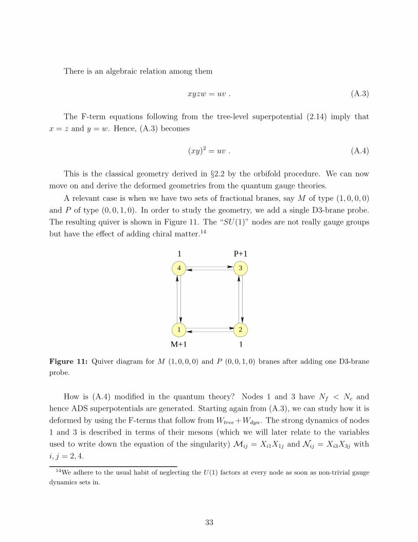
There is an algebraic relation among them

xyzw = uv . (A.3)

The F-term equations following from the tree-level superpotential (2.14) imply that

x = z and y = w. Hence, (A.3) becomes

(xy)2 = uv . (A.4)

This is the classical geometry derived in §2.2 by the orbifold procedure. We can now

move on and derive the deformed geometries from the quantum gauge theories.

A relevant case is when we have two sets of fractional branes, say M of type (1, 0, 0, 0)

and P of type (0, 0, 1, 0). In order to study the geometry, we add a single D3-brane probe.

The resulting quiver is shown in Figure 11. The “SU(1)” nodes are not really gauge groups

but have the effect of adding chiral matter.14

1

1M+1

P+1

1 2

34

Figure 11: Quiver diagram for M (1, 0, 0, 0) and P (0, 0, 1, 0) branes after adding one D3-brane

probe.

How is (A.4) modified in the quantum theory? Nodes 1 and 3 have Nf < Nc and

hence ADS superpotentials are generated. Starting again from (A.3), we can study how it is

deformed by using the F-terms that follow from Wtree +Wdyn. The strong dynamics of nodes

1 and 3 is described in terms of their mesons (which we will later relate to the variables

used to write down the equation of the singularity) Mij = Xi1X1j and Nij = Xi3X3j with

i, j = 2, 4.

14We adhere to the usual habit of neglecting the U(1) factors at every node as soon as non-trivial gauge

dynamics sets in.

33

Adding the tree-level and dynamical superpotentials, we obtain

W = h (M22N22 + M44N44 −M24M42 −N24N42) +

+ (M − 1)

(

Λ3M+11

detM

)1

M−1

+ (P − 1)

(

Λ3P+13

detN

)1

P−1

. (A.5)

The F-terms altogether imply

detM =

(

Λ3M+11

hM−1

)

1M

= ǫ1 , detN =

(

Λ3P+13

hP−1

)

1P

= ǫ3 (A.6)

and

M22 = N44 , M44 = N22 . (A.7)

We have the following identifications

x = M22 , y = N22 , z = N44 ≡ x , w = M44 ≡ y (A.8)

where we have used (A.7), and

u = M42N24 , v = M24N42 . (A.9)

We note that (A.6) implies that M24M42 = M22M44 − ǫ1 ≡ xy − ǫ1, and N24N42 =

N22N44 − ǫ3 ≡ xy − ǫ3 . Using again (A.7), we conclude that the deformed geometry

corresponds to

(xy − ǫ1)(xy − ǫ3) = uv . (A.10)

For generic deformation parameters ǫ1 and ǫ3, the above geometry is completely regular.

However, for ǫ1 = ǫ3 it has a line of A1 singularities on the locus defined by xy − ǫ1 = 0.

On the locus of singular points, which contain small IP1s, we can then add the fractional

branes of N = 2 kind. This corresponds to the class ii) vacua discussed in §5. Note that the

simplest way to satisfy the relation ǫ1 = ǫ3 is when the ranks and scales are equal, P = M

and Λ1 = Λ3.

We can use these results also to determine the deformation of the geometry once we

are in the baryonic branch for both nodes 1 and 3, which corresponds to the class i) vacua.

This leaves a single SU(M) confining gauge group, node 2, behind. As argued in §5.1, this

is expected to correspond to a single deformation. In fact, after rotating the quiver such

that nodes are relabeled according to (1, 2, 3, 4) → (4, 1, 2, 3), the deformation follows from

setting P = 0 in our previous analysis. Hence, (A.10) reduces to

(xy − ǫ)(xy) = uv . (A.11)

34

It is straightforward to check that there is a remaining conifold singularity in the moduli

space. From a field theory point of view, this is expected to be manifest when the dynamical

scale of the leftover node goes to infinity (equivalently when ǫ → ∞). This corresponds to

studying the theory at energy scales much lower than Λ2. Using rescaled variables x = ǫ1/2x

and y = ǫ1/2y, (A.11) becomes the conifold equation xy = uv.

B. Toric geometry, (p, q) webs and complex deformations

This appendix presents basic notions about toric singularities and their description in terms

of (p, q) webs. The goal is to provide a brief description of practical rules necessary to get

an intuitive understanding of the basic geometric features of a singularity and its possible

deformations. We refer the reader to [55, 56, 57] for more detailed presentations of toric

geometry and to [58, 59] for comprehensive expositions of the connections between web

diagrams and toric geometry. These ideas are not crucial for understanding the current

paper but are useful for identifying the cycles over which branes are wrapped. They also

simplify the study of generalizations of our model.

A d-complex dimensional toric variety V d is a generalization of a complex projective

space, defined as

V d = (Cn − F )/C∗(n−d) (B.1)

in which we quotient by (n−d) C∗ actions and we remove a set of points F in order for such

quotient to be well defined. The action of C∗(n−d) on the Cn coordinates is defined by (n−d)

charge vectors Qa as

λa : (x1, . . . , xn) → (λQa1

a x1, . . . , λQa

na xn), a = 1, . . . , n − d . (B.2)

The charges can be arranged into a matrix Q = (Qai ). This approach to toric varieties

is known as the holomorphic quotient.

Alternatively, we can perform the quotient by C∗(n−d) in two steps, decomposing each

C∗ = IR+ × U(1). This approach is called the symplectic quotient. We first fix the IR+(n−d)

levels via a moment map

n∑

i=1

Qia|xi|2 = ξa, a = 1, . . . , n − d (B.3)

for some real parameters ξa. We refer to these equations D-terms. This is because they are

actually the D-terms of an N = 2 gauged linear sigma model (GLSM) with target space Cn

which reduces in the infrared to a non-linear sigma model whose target space is the toric

variety V d [60].

35

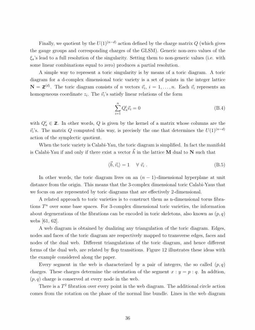
Finally, we quotient by the U(1)(n−d) action defined by the charge matrix Q (which gives

the gauge groups and corresponding charges of the GLSM). Generic non-zero values of the

ξa’s lead to a full resolution of the singularity. Setting them to non-generic values (i.e. with

some linear combinations equal to zero) produces a partial resolution.

A simple way to represent a toric singularity is by means of a toric diagram. A toric

diagram for a d-complex dimensional toric variety is a set of points in the integer lattice

N = ZZ(d). The toric diagram consists of n vectors ~vi, i = 1, . . . , n. Each ~vi represents an

homogeneous coordinate zi. The ~vi’s satisfy linear relations of the form

n∑

i=1

Qia~vi = 0 (B.4)

with Qia ∈ ZZ. In other words, Q is given by the kernel of a matrix whose columns are the

~vi’s. The matrix Q computed this way, is precisely the one that determines the U(1)(n−d)

action of the symplectic quotient.

When the toric variety is Calabi-Yau, the toric diagram is simplified. In fact the manifold

is Calabi-Yau if and only if there exist a vector ~h in the lattice M dual to N such that

〈~h,~vi〉 = 1 ∀ ~vi . (B.5)

In other words, the toric diagram lives on an (n − 1)-dimensional hyperplane at unit

distance from the origin. This means that the 3-complex dimensional toric Calabi-Yaus that

we focus on are represented by toric diagrams that are effectively 2-dimensional.

A related approach to toric varieties is to construct them as n-dimensional torus fibra-

tions T n over some base spaces. For 3-complex dimensional toric varieties, the information

about degenerations of the fibrations can be encoded in toric skeletons, also known as (p, q)

webs [61, 62].

A web diagram is obtained by dualizing any triangulation of the toric diagram. Edges,

nodes and faces of the toric diagram are respectively mapped to transverse edges, faces and

nodes of the dual web. Different triangulations of the toric diagram, and hence different

forms of the dual web, are related by flop transitions. Figure 12 illustrates these ideas with

the example considered along the paper.

Every segment in the web is characterized by a pair of integers, the so called (p, q)

charges. These charges determine the orientation of the segment x : y = p : q. In addtion,

(p, q) charge is conserved at every node in the web.

There is a T 2 fibration over every point in the web diagram. The additional circle action

comes from the rotation on the phase of the normal line bundle. Lines in the web diagram

36

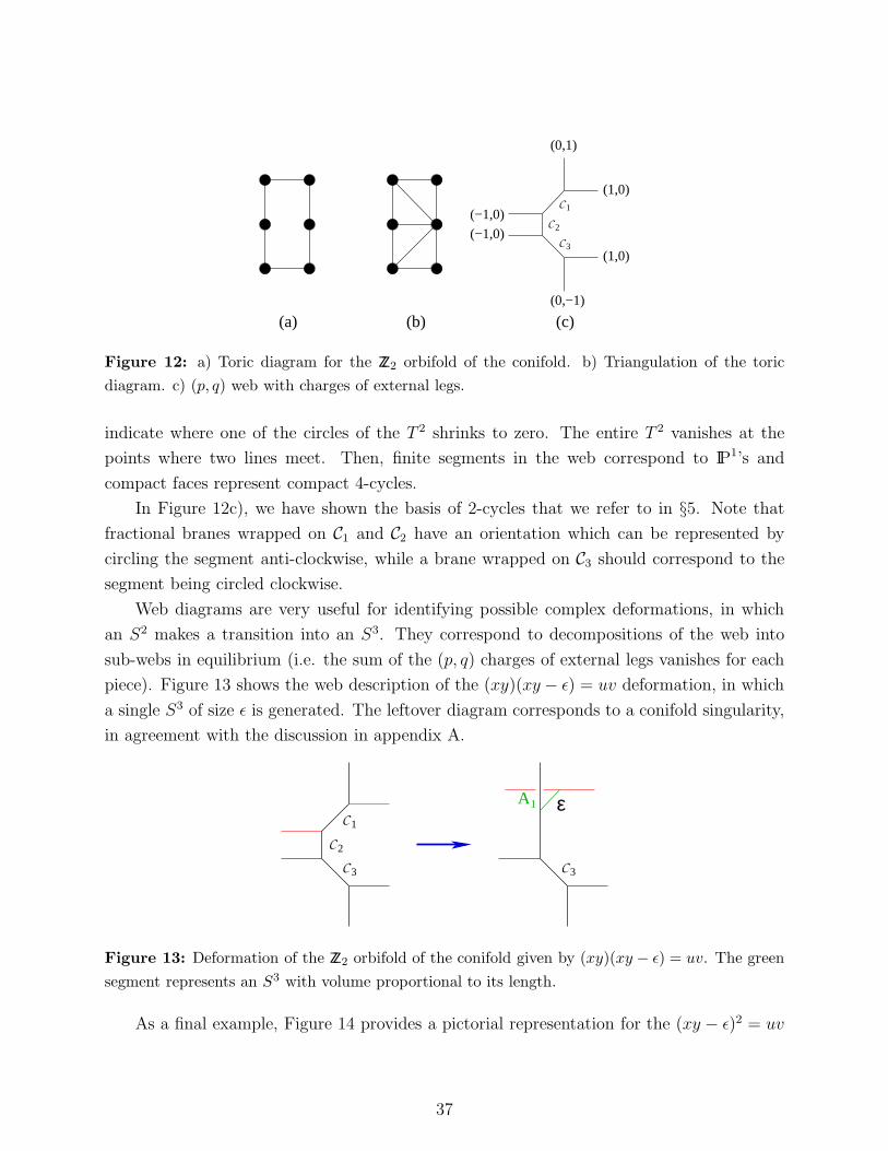
(1,0)

(1,0)

(0,−1)

(0,1)

(c)

(−1,0)

(−1,0)

C1

C3

C2

(b)(a)

Figure 12: a) Toric diagram for the ZZ2 orbifold of the conifold. b) Triangulation of the toric

diagram. c) (p, q) web with charges of external legs.

indicate where one of the circles of the T 2 shrinks to zero. The entire T 2 vanishes at the

points where two lines meet. Then, finite segments in the web correspond to IP1’s and

compact faces represent compact 4-cycles.

In Figure 12c), we have shown the basis of 2-cycles that we refer to in §5. Note that

fractional branes wrapped on C1 and C2 have an orientation which can be represented by

circling the segment anti-clockwise, while a brane wrapped on C3 should correspond to the

segment being circled clockwise.

Web diagrams are very useful for identifying possible complex deformations, in which

an S2 makes a transition into an S3. They correspond to decompositions of the web into

sub-webs in equilibrium (i.e. the sum of the (p, q) charges of external legs vanishes for each

piece). Figure 13 shows the web description of the (xy)(xy − ǫ) = uv deformation, in which

a single S3 of size ǫ is generated. The leftover diagram corresponds to a conifold singularity,

in agreement with the discussion in appendix A.

C 1

C 3

C 2

C 3

ε1A

Figure 13: Deformation of the ZZ2 orbifold of the conifold given by (xy)(xy − ǫ) = uv. The green

segment represents an S3 with volume proportional to its length.

As a final example, Figure 14 provides a pictorial representation for the (xy − ǫ)2 = uv

37

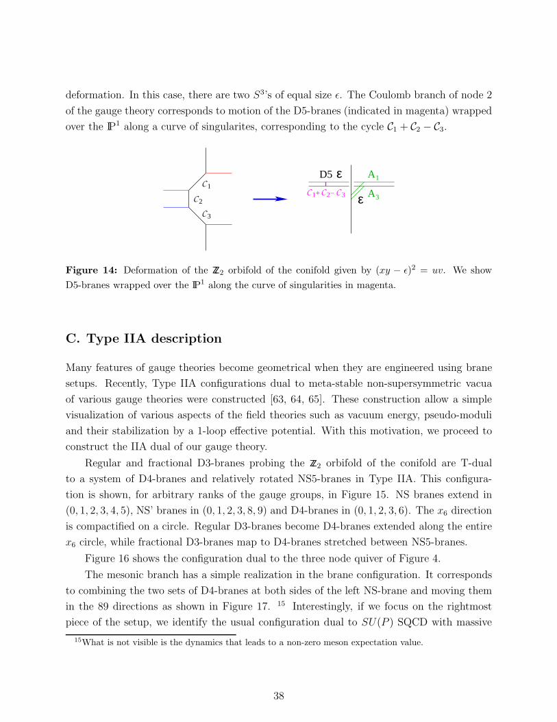
deformation. In this case, there are two S3’s of equal size ǫ. The Coulomb branch of node 2

of the gauge theory corresponds to motion of the D5-branes (indicated in magenta) wrapped

over the IP1 along a curve of singularites, corresponding to the cycle C1 + C2 − C3.

C1

C3

C2

1A

3A

D5

ε

ε+1 C C3C 2−

Figure 14: Deformation of the ZZ2 orbifold of the conifold given by (xy − ǫ)2 = uv. We show

D5-branes wrapped over the IP1 along the curve of singularities in magenta.

C. Type IIA description

Many features of gauge theories become geometrical when they are engineered using brane

setups. Recently, Type IIA configurations dual to meta-stable non-supersymmetric vacua

of various gauge theories were constructed [63, 64, 65]. These construction allow a simple

visualization of various aspects of the field theories such as vacuum energy, pseudo-moduli

and their stabilization by a 1-loop effective potential. With this motivation, we proceed to

construct the IIA dual of our gauge theory.

Regular and fractional D3-branes probing the ZZ2 orbifold of the conifold are T-dual

to a system of D4-branes and relatively rotated NS5-branes in Type IIA. This configura-

tion is shown, for arbitrary ranks of the gauge groups, in Figure 15. NS branes extend in

(0, 1, 2, 3, 4, 5), NS’ branes in (0, 1, 2, 3, 8, 9) and D4-branes in (0, 1, 2, 3, 6). The x6 direction

is compactified on a circle. Regular D3-branes become D4-branes extended along the entire

x6 circle, while fractional D3-branes map to D4-branes stretched between NS5-branes.

Figure 16 shows the configuration dual to the three node quiver of Figure 4.

The mesonic branch has a simple realization in the brane configuration. It corresponds

to combining the two sets of D4-branes at both sides of the left NS-brane and moving them

in the 89 directions as shown in Figure 17. 15 Interestingly, if we focus on the rightmost

piece of the setup, we identify the usual configuration dual to SU(P ) SQCD with massive

15What is not visible is the dynamics that leads to a non-zero meson expectation value.

38

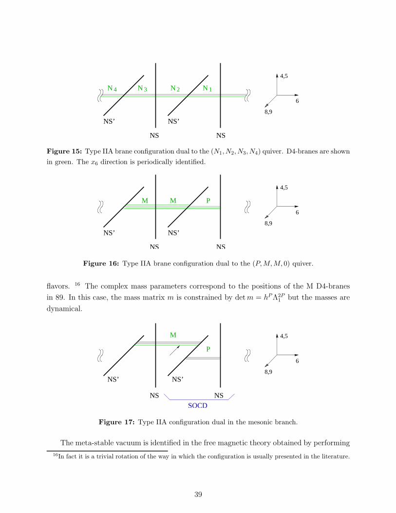
4,5

6

8,9

N 1N 2N 3N 4

NS

NS’

NS

NS’

Figure 15: Type IIA brane configuration dual to the (N1, N2, N3, N4) quiver. D4-branes are shown

in green. The x6 direction is periodically identified.

4,5

6

8,9

M M P

NS

NS’

NS

NS’

Figure 16: Type IIA brane configuration dual to the (P,M,M, 0) quiver.

flavors. 16 The complex mass parameters correspond to the positions of the M D4-branes

in 89. In this case, the mass matrix m is constrained by det m = hP Λ2P1 but the masses are

dynamical.

4,5

6

8,9

P

NS’NS’

NSNS

M

SQCD

Figure 17: Type IIA configuration dual in the mesonic branch.

The meta-stable vacuum is identified in the free magnetic theory obtained by performing

16In fact it is a trivial rotation of the way in which the configuration is usually presented in the literature.

39

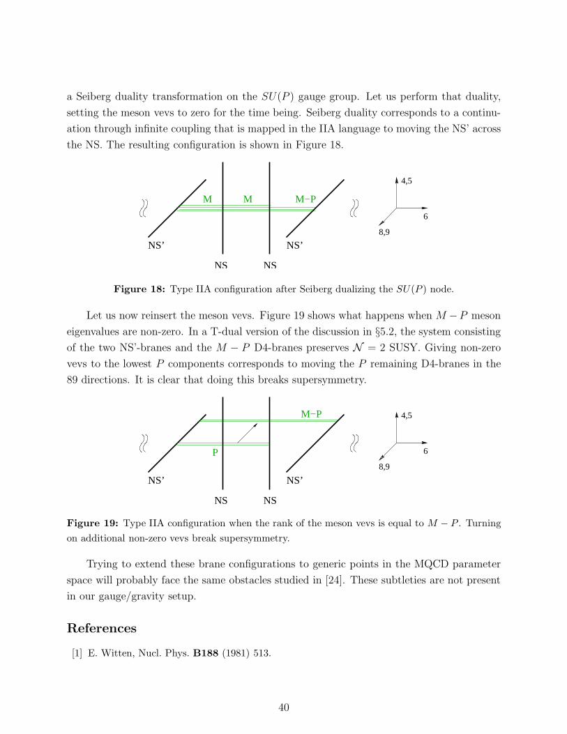
a Seiberg duality transformation on the SU(P ) gauge group. Let us perform that duality,

setting the meson vevs to zero for the time being. Seiberg duality corresponds to a continu-

ation through infinite coupling that is mapped in the IIA language to moving the NS’ across

the NS. The resulting configuration is shown in Figure 18.

4,5

6

8,9

M M

NS

NS’NS’

NS

M−P

Figure 18: Type IIA configuration after Seiberg dualizing the SU(P ) node.

Let us now reinsert the meson vevs. Figure 19 shows what happens when M −P meson

eigenvalues are non-zero. In a T-dual version of the discussion in §5.2, the system consisting

of the two NS’-branes and the M − P D4-branes preserves N = 2 SUSY. Giving non-zero

vevs to the lowest P components corresponds to moving the P remaining D4-branes in the

89 directions. It is clear that doing this breaks supersymmetry.

4,5

6

8,9

NS

NS’NS’

NS

M−P

P

Figure 19: Type IIA configuration when the rank of the meson vevs is equal to M − P . Turning

on additional non-zero vevs break supersymmetry.

Trying to extend these brane configurations to generic points in the MQCD parameter

space will probably face the same obstacles studied in [24]. These subtleties are not present

in our gauge/gravity setup.

References

[1] E. Witten, Nucl. Phys. B188 (1981) 513.

40

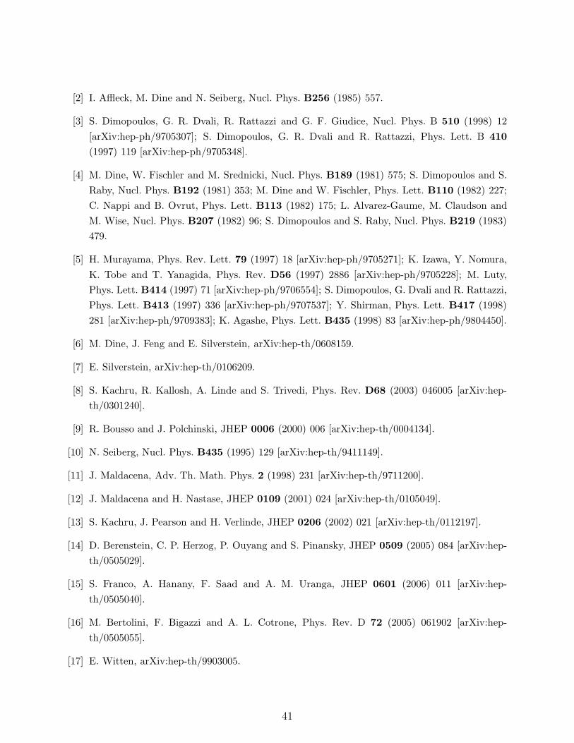
[2] I. Affleck, M. Dine and N. Seiberg, Nucl. Phys. B256 (1985) 557.

[3] S. Dimopoulos, G. R. Dvali, R. Rattazzi and G. F. Giudice, Nucl. Phys. B 510 (1998) 12

[arXiv:hep-ph/9705307]; S. Dimopoulos, G. R. Dvali and R. Rattazzi, Phys. Lett. B 410

(1997) 119 [arXiv:hep-ph/9705348].

[4] M. Dine, W. Fischler and M. Srednicki, Nucl. Phys. B189 (1981) 575; S. Dimopoulos and S.

Raby, Nucl. Phys. B192 (1981) 353; M. Dine and W. Fischler, Phys. Lett. B110 (1982) 227;

C. Nappi and B. Ovrut, Phys. Lett. B113 (1982) 175; L. Alvarez-Gaume, M. Claudson and

M. Wise, Nucl. Phys. B207 (1982) 96; S. Dimopoulos and S. Raby, Nucl. Phys. B219 (1983)

479.

[5] H. Murayama, Phys. Rev. Lett. 79 (1997) 18 [arXiv:hep-ph/9705271]; K. Izawa, Y. Nomura,

K. Tobe and T. Yanagida, Phys. Rev. D56 (1997) 2886 [arXiv:hep-ph/9705228]; M. Luty,

Phys. Lett. B414 (1997) 71 [arXiv:hep-ph/9706554]; S. Dimopoulos, G. Dvali and R. Rattazzi,

Phys. Lett. B413 (1997) 336 [arXiv:hep-ph/9707537]; Y. Shirman, Phys. Lett. B417 (1998)

281 [arXiv:hep-ph/9709383]; K. Agashe, Phys. Lett. B435 (1998) 83 [arXiv:hep-ph/9804450].

[6] M. Dine, J. Feng and E. Silverstein, arXiv:hep-th/0608159.

[7] E. Silverstein, arXiv:hep-th/0106209.

[8] S. Kachru, R. Kallosh, A. Linde and S. Trivedi, Phys. Rev. D68 (2003) 046005 [arXiv:hep-

th/0301240].

[9] R. Bousso and J. Polchinski, JHEP 0006 (2000) 006 [arXiv:hep-th/0004134].

[10] N. Seiberg, Nucl. Phys. B435 (1995) 129 [arXiv:hep-th/9411149].

[11] J. Maldacena, Adv. Th. Math. Phys. 2 (1998) 231 [arXiv:hep-th/9711200].

[12] J. Maldacena and H. Nastase, JHEP 0109 (2001) 024 [arXiv:hep-th/0105049].

[13] S. Kachru, J. Pearson and H. Verlinde, JHEP 0206 (2002) 021 [arXiv:hep-th/0112197].

[14] D. Berenstein, C. P. Herzog, P. Ouyang and S. Pinansky, JHEP 0509 (2005) 084 [arXiv:hep-

th/0505029].

[15] S. Franco, A. Hanany, F. Saad and A. M. Uranga, JHEP 0601 (2006) 011 [arXiv:hep-

th/0505040].

[16] M. Bertolini, F. Bigazzi and A. L. Cotrone, Phys. Rev. D 72 (2005) 061902 [arXiv:hep-

th/0505055].

[17] E. Witten, arXiv:hep-th/9903005.

41

[18] K. Intriligator and N. Seiberg, JHEP 0602 (2006) 031 [arXiv:hep-th/0512347].

[19] A. Brini and D. Forcella, JHEP 0606 (2006) 050 [arXiv:hep-th/0603245].

[20] B. Florea, S. Kachru, J. McGreevy and N. Saulina, arXiv:hep-th/0610003.

[21] R. Argurio, M. Bertolini, C. Closset and S. Cremonesi, JHEP 0609 (2006) 030 [arXiv:hep-

th/0606175].

[22] S. Franco and A. M. Uranga, JHEP 0606 (2006) 031 [arXiv:hep-th/0604136].

[23] I.R. Klebanov and M. Strassler, JHEP 0008 (2000) 052 [arXiv:hep-th/0007191].

[24] I. Bena, E. Gorbatov, S. Hellerman, N. Seiberg and D. Shih, arXiv:hep-th/0608157.

[25] S. Kachru et al, JCAP 0310 (2003) 013 [arXiv:hep-th/0308055].

[26] O. DeWolfe, S. Kachru and H. Verlinde, JHEP 0405 (2004) 017 [arXiv:hep-th/0403123].

[27] K. Intriligator, N. Seiberg and D. Shih, JHEP 0604 (2006) 021 [arXiv:hep-th/0602239].

[28] H. Ooguri and Y. Ookouchi, arXiv:hep-th/0606061.

[29] T. Banks, arXiv:hep-ph/0606313.

[30] S. Forste, arXiv:hep-th/0608036.

[31] A. Amariti, L. Girardello and A. Mariotti, arXiv:hep-th/0608063.

[32] N. Seiberg, Phys. Rev. D49 (1994) 6857 [arXiv:hep-th/9402044].

[33] A. M. Uranga, JHEP 9901 (1999) 022 [arXiv:hep-th/9811004].

[34] C. Johnson, A. Peet and J. Polchinski, Phys. Rev. D61 (2000) 086001 [arXiv:hep-th/9911161].

[35] I. Affleck, M. Dine and N. Seiberg, Nucl. Phys. B241 (1984) 493.

[36] I. R. Klebanov and A. A. Tseytlin, Nucl. Phys. B 578 (2000) 123 [arXiv:hep-th/0002159].

[37] M. J. Strassler, arXiv:hep-th/0505153.

[38] S. Franco, Y. He, C. Herzog and J. Walcher, Phys. Rev. D70 (2004) 046006 [arXiv:hep-

th/0402120].

[39] C. P. Herzog, Q. J. Ejaz and I. R. Klebanov, JHEP 0502 (2005) 009 [arXiv:hep-th/0412193].

[40] A. Dymarsky, I. Klebanov and N. Seiberg, JHEP 0601 (2006) 155 [arXiv:hep-th/0511254].

42

[41] S. Giddings, S. Kachru and J. Polchinski, Phys. Rev. D66 (2002) 106006 [arXiv:hep-

th/0105097].

[42] S. Gubser, C. Herzog and I. Klebanov, JHEP 0409 (2004) 036 [arXiv:hep-th/0405282].

[43] R. Gopakumar and C. Vafa, Adv. Th. Math. Phys. 3 (1999) 1415 [arXiv:hep-th/9811131].

[44] C. Vafa, J. Math. Phys. 42 (2001) 2798 [arXiv:hep-th/0008142].

[45] S. Gukov, C. Vafa and E. Witten, Nucl. Phys. B584 (2000) 69 [arXiv:hep-th/9906070].

[46] T. Taylor, G. Veneziano and S. Yankielowicz, Nucl. Phys. B218 (1983) 493.

[47] D. Berenstein, arXiv:hep-th/0303230.

[48] E. Imeroni and A. Lerda, JHEP 0312 (2003) 051 [arXiv:hep-th/0310157].

[49] I. Klebanov and E. Witten, Nucl. Phys. B536 (1998) 199 [arXiv:hep-th/9807080].

[50] R. C. Myers, JHEP 9912 (1999) 022 [arXiv:hep-th/9910053].

[51] J. Polchinski, String theory. Vol 2: Superstring theory and beyond, Cambridge University Press

(1998), pp. 169-170.

[52] M. Grana and J. Polchinski, Phys. Rev. D63 (2001) 026001 [arXiv:hep-th/0009211].

[53] M. Bertolini, P. Di Vecchia, M. Frau, A. Lerda, R. Marotta and I. Pesando, JHEP 0102 (2001)

014 [arXiv:hep-th/0011077].

[54] R. Argurio, G. Ferretti and C. Petersson, JHEP 0603 (2006) 043 [arXiv:hep-th/0601180].

[55] W. Fulton. Introduction to toric varieties. Princeton University Press, 1993.

[56] P. S. Aspinwall, B. R. Greene and D. R. Morrison, Nucl. Phys. B 416 (1994) 414 [arXiv:hep-

th/9309097].

[57] D. R. Morrison and M. Ronen Plesser, Nucl. Phys. B 440 (1995) 279 [arXiv:hep-th/9412236].

[58] N. C. Leung and C. Vafa, Adv. Theor. Math. Phys. 2 (1998) 91 [arXiv:hep-th/9711013].

[59] S. Franco and A. Hanany, JHEP 0304 (2003) 043 [arXiv:hep-th/0207006].

[60] E. Witten, Nucl. Phys. B 403 (1993) 159 [arXiv:hep-th/9301042].

[61] O. Aharony and A. Hanany, Nucl. Phys. B 504 (1997) 239 [arXiv:hep-th/9704170].

[62] O. Aharony, A. Hanany and B. Kol, JHEP 9801 (1998) 002 [arXiv:hep-th/9710116].

43

[63] H. Ooguri and Y. Ookouchi, arXiv:hep-th/0607183.

[64] S. Franco, I. Garcia-Etxebarria and A. M. Uranga, arXiv:hep-th/0607218.

[65] C. Ahn, arXiv:hep-th/0608160.

44