Gauge Theory Gravity with GeometricCalculus

David Hestenes1

Department of Physics and AstronomyArizona State University, Tempe, Arizona 85287-1504

A new gauge theory of gravity on flat spacetime has recently been developedby Lasenby, Doran, and Gull. Einstein’s principles of equivalence and generalrelativity are replaced by gauge principles asserting, respectively, local rota-tion and global displacement gauge invariance. A new unitary formulation ofEinstein’s tensor illuminates long-standing problems with energy-momentumconservation in general relativity. Geometric calculus provides many simpli-fications and fresh insights in theoretical formulation and physical applicationsof the theory.

I. Introduction

More than a decade before the advent of Einstein’s general theory of relativity(GR), and after a lengthy and profound analysis of the relation between physicsand geometry [1], Henri Poincare concluded that:

“One geometry cannot be more true than another; it can onlybe more convenient. Now, Euclidean geometry is and will remain,the most convenient. . . . What we call a straight line in astronomyis simply the path of a ray of light. If, therefore, we were to discovernegative parallaxes, or to prove that all parallaxes are higher than acertain limit, we should have a choice between two conclusions: wecould give up Euclidean geometry, or modify the laws of optics, andsuppose that light is not rigorously propagated in a straight line. Itis needless to add that every one would look upon this solution asthe more advantageous.” [italics added]

Applied to GR, this amounts to claiming that any curved space formulation ofphysics can be replaced by an equivalent and simpler flat space formulation.Ironically, the curved space formulation has been preferred by nearly everyonesince the inception of GR, and many attempts at alternative flat space formula-tions have failed to exhibit the simplicity anticipated by Poincare. One wondersif the trend might have been different if Poincare were still alive to promote hisview when GR made its spectacular appearance on the scene.

A dramatic new twist on the physics-geometry connection has been intro-duced by Cambridge physicists Lasenby, Doran, and Gull with their flat space

1electronic mail:hestenes@asu.edu

1

alternative to GR called gauge theory gravity (GTG) [2, 3]. With geometric cal-culus (GC) as an essential tool, they clarify the foundations of GR and providemany examples of computational simplifications in the flat space gauge theory.All this amounts to compelling evidence that Poincare was right in the firstplace [4].

The chief innovation of GTG is a displacement gauge principle that assertsglobal homogeneity of spacetime. This is a new kind of gauge principle thatclarifies and revitalizes Einstein’s general relativity principle by cleanly sep-arating arbitrary coordinate transformations from physically significant fieldtransformations. GTG also posits a rotation gauge principle of standard typein nonAbelian gauge theory. The present account is unique in interpretingthis principle as a realization of Einstein’s Equivalence Principle asserting localisotropy of spacetime. With rotation gauge equivalence and displacement gaugeequivalence combined, GTG synthesizes Einstein’s principles of equivalence andgeneral relativity into a new general principle of gauge equivalence.

A unique consequence of GTG, announced here for the first time, is theexistence of a displacement gauge invariant energy-momentum conservation law.

Many previous attempts to formulate a flat space alternative to GR are awk-ward and unconvincing. The most noteworthy alternative is the self-consistentfield theory of a massless spin-2 particle (the graviton) [5]. That is a gaugetheory with local Lorentz rotations as gauge transformations. However, it lacksthe simplicity brought by the Displacement Gauge Principle in GTG.

GTG is also unique in its use of geometric calculus (GC). It is, of course,possible to reformulate GTG in terms of more standard mathematics, but at theloss of much of the theory’s elegance and simplicity. Indeed, GC is so uniquelysuited to GTG it is doubtful that the theory would have developed without it.That should be evident in the details that follow.

This is the third in a series of articles promoting geometric algebra (GA)as a unified mathematical language for physics [6, 7]. Here, GA is extendedto a geometric calculus (GC) that includes the tools of differential geometryneeded for Einstein’s theory of general relativity (GR) on flat spacetime. Mypurpose is to demonstrate the unique geometrical insight and computationalpower that GC brings to GR, and to introduce mathematical tools that areready for use in teaching and research. This provides the last essential piece fora comprehensive geometric algebra and calculus expressly designed to serve thepurposes of theoretical physics [8, 9].

The preceding article [7] (hereafter referred to as GA2) is a preferred prereq-uisite, but to make the present article reasonably self-contained, a summary ofessential concepts, notations and results from GA2 is included. Of course, priorfamiliarity with standard treatments of GR will be helpful as well. However, forstudents who have mastered GA2, the present article may serve as a suitableentree to GR. As a comprehensive treatment of GR is not possible here, it willbe necessary for students to coordinate study of this article with one of themany fine textbooks on GR. In a course for undergraduates, the textbook byd’Inverno [10] would be a good choice for that purpose. In my experience, thechallenge of reformulating GR in terms of GC is a great stimulus to student

2

learning.As emphasized in GA2, one great advantage of adopting GC as a unified

language for physics is that it eliminates unnecessary language and conceptualbarriers between classical, quantum and relativistic physics. I submit that thesimplifications introduced by GC are essential to fitting an adequate treatmentof GR into the undergraduate physics curriculum. It is about time for blackholes and cosmology to be incorporated into the standard curriculum. Althoughspace limitations preclude addressing such topics here, the mathematical toolsintroduced are sufficient to treat any topic with GC, and more details are givenin a recent book [2].

Recognition that GR should be formulated as a gauge theory has been along time coming, and, though it is often discussed in the research literature[11], it is still relegated to a subtopic in most GR textbooks, in part becausethe standard covariant tensor formalism is not well suited to gauge theory.Still less is it recognized that there is a connection between gravitational gaugetransformations and Einstein’s Principle of Equivalence. Gauge theory is theone strong conceptual link between GR and quantum mechanics, if only becauseit is essential for incorporating the Dirac equation into GR. This is sufficientreason to bring gauge theory to the fore in the formulation of GR.

This article demonstrates that GC is conceptually and computationally idealfor a gauge theory approach to GR — conceptually ideal, because concepts ofvector and spinor are integrated by the geometric product in its mathematicalfoundations — computationally ideal, because computations can be done with-out coordinates. Much of this article is devoted to demonstrating the efficiencyof GC in computations. The GC approach is pedagogically efficient as well, asit develops GR by a straightforward generalization of Special Relativity usingmathematical tools already well developed in GA2.

Essential mathematical tools introduced in GA2 are summarized in SectionII, though mastery of GA2 may be necessary to understand the more subtleaspects of the theory. Section III extends the tool kit to unique mathematicaltools for linear algebra and induced transformations on manifolds. These toolsare indispensible for GTG and useful throughout the rest of physics.

Section IV introduces the gauge principles of GTG and shows how they gen-erate an induced geometry on spacetime that is mathematically equivalent tothe Riemannian geometry of GR. Some facility with GC is needed to appreci-ate how it streamlines the formulation, analysis and application of differentialgeometry, so the more subtle derivations have been relegated to appendices.

Section V discusses the formulation of field equations and equations of mo-tion in GTG. Besides standard results of GR, it includes a straightforwardextension of spinor methods in GA2 to treat gravitational precession and grav-itational interactions in the Dirac equation.

Section VI discusses simplifications that GTG brings to the formulation andanalysis of solutions to the gravitational field equations, in particular, motionin the field of a black hole.

Section VII introduces a new split of the Einstein tensor to produce a newdefinition for the energy-momentum tensor and a general energy-momentum

3

conservation law.Section VIII summarizes the basic principles of GTG and discusses their

status in comparison with Newton’s Laws as universal principles for physics.

II. Spacetime Algebra Background

This section reviews and extends concepts, notations and results from GA2 thatwill be applied and generalized in this paper. Our primary mathematical toolis the the real Spacetime Algebra (STA). One great advantage of STA is thatit enables coordinate-free representation and computation of physical systemsand processes. Another is that it incorporates the spinors of quantum me-chanics along with the tensors (in coordinate-free form) of classical field theory.Some results from GA2 are summarized below without proof, and the readeris encouraged to consult GA2 for more details. Other results from GA2 willbe recalled as needed. The reader should note that most of GA2 carries overwithout change; the essential differences all come from a generalized gauge con-cept of differentiation. We show in subsequent sections that the gauge covariantderivative accommodates curved-space geometry in flat space to achieve a flat-space gauge theory of gravity. However, the accomodation is subtle, so it wasdiscovered only recently.

A. STA elements and operations

For physicists familiar with the Dirac matrix algebra, the quickest approachto STA is by reinterpreting the Dirac matrices as an orthonormal basis γµ;µ =0, 1, 2, 3 for a 4D real Minkowski vector space V4 with signature specified bythe rules:

γ20 = 1 and γ2

1 = γ22 = γ2

3 = −1 . (1)

Note that the scalar 1 in these equations would be replaced by the identitymatrix if the γµ were Dirac matrices. Thus, (1) is no mere shorthand for matrixequations but a defining relation of vectors to scalars that encodes spacetimesignature in algebraic form.

The frame γµ generates an associative geometric algebra that is isomorphicto the Dirac algebra. The product γµγν of two vectors is called the geometricproduct. The usual inner product of vectors is defined by

γµ · γν ≡ 12 (γµγν + γνγµ) = ηµδµν , (2)

where ηµ = γ2µ is the signature indicator. The outer product

γµ ∧ γν ≡ 12 (γµγν − γνγµ) = −γν ∧ γµ , (3)

defines a new entity called a bivector (or 2-vector), which can be interpreted asa directed plane segment representing the plane containing the two vectors.

STA is the geometric algebra G4 = G(V4) generated by V4. A full basis forthe algebra is given by the set:

4

1 γµ γµ ∧ γν γµi i1 scalar 4 vectors 6 bivectors 4 trivectors 1 pseudoscalargrade 0 grade 1 grade 2 grade 3 grade 4

where the unit pseudoscalar

i ≡ γ0γ1γ2γ3 (4)

squares to −1, anticommutes with all odd grade elements and commutes witheven grade elements. Thus, G4 is a linear space of dimension 1+4+6+4+1 =24 = 16.

A generic element of G4 is called a multivector. Any multivector can beexpressed as a linear combination of the basis elements. For example, a bivectorF has the expansion

F = 12Fµνγµ ∧ γν , (5)

with its “scalar components” Fµν in the usual tensorial form. For components,we use the usual tensor algebra conventions for raising and lowering indices andsumming over repeated upper and lower index pairs.

Any multivector M can be written in the expanded forms

M = α + a + F + bi + βi =4∑

k=0

〈M〉k, (6)

where α = 〈M〉0 and β are scalars, a = 〈M〉1 and b are vectors, and F = 〈M〉2is a bivector, while bi = 〈M〉3 is a trivector (or pseudovector) and βi = 〈M〉4 isa pseudoscalar. It is often convenient to drop the subscript on the scalar partso 〈M〉 = 〈M〉0. The scalar part behaves like the “trace” in matrix algebra; forexample, 〈MN〉 = 〈NM〉 for arbitrary multivectors M and N . A multivectoris said to be even if the grades of its nonvanishing components are all even. Theeven multivectors compose the even subalgebra of G4, which is, of course, closedunder the geometric product.

Coordinate-free computations are facilitated by various definitions. The op-eration of reversion reverses the order in a product of vectors, so for vectorsa, b, c it is defined by

(abc)˜= cba . (7)

It follows for any multivector M in the expanded form (6) that the reverse Mis given by

M = α + a − F − bi + βi . (8)

Computations are also facilitated by defining various products in terms of thefundamental geometric product.

5

The inner and outer products of vectors, (2) and (3) can be generalized toarbitrary multivectors as follows. For A = 〈A〉r and B = 〈B〉s of grades r, s ≥ 0,inner and outer products can be defined by

A · B ≡ 〈AB〉|r−s|, A ∧ B ≡ 〈AB〉r+s . (9)

Coordinate-free manipulations are facilitated by a system of identities involvinginner and outer products [8]. These identities generalize to arbitrary dimen-sions the well-known identities for dot and cross products in ordinary 3D vectoralgebra. Only a few of the most commonly used identities are listed here. Fora vector a, the geometric product is related to inner and outer products by

aB = a · B + a ∧ B . (10)

For vectors a, b, c the most commonly used identity is

a · (b ∧ c) = (a · b)c − (a · c)b = a · b c − a · c b . (11)

This is a special case of

a · (b ∧ B) = a · b B − b ∧ (a · B) (12)

for grade(B) ≥ 2, and we have a related identity

a · (b · B) = (a ∧ b) · B . (13)

We also need the commutator product

A × B ≡ 12 (AB − BA). (14)

This is especially useful when A is a bivector. Then we have the identity

AB = A · B + A × B + A ∧ B, (15)

which should be compared with (10). For s = grade(B), it is easy to prove thatthe three terms on the right side of (15) have grades s− 2, s, s + 2 respectively.

Note the dropping of parentheses on the right hand side of (11). To reducethe number of parentheses in an expression, we sometimes use a precedence con-vention, which allows that inner, outer and commutator products take prece-dence over the geometric product in ambiguous expressions.

Finally, we note that the concept of duality, which appears throughout math-ematics, has a very simple realization in GA. The dual of any multivector issimply obtained by multiplying it by the pseudoscalar i (or, sometimes, by ascalar multiple thereof). Thus, in (6) the trivector bi is the dual of the vectorb. Inner and outer products are related by the duality identities

a · (Bi) = (a ∧ B)i , a ∧ (Bi) = (a · B)i . (16)

6

B. Lorentz rotations and rotors

A complete treatment of Lorentz transformations is given in GA2. We areconcerned here only with transformations continuously connected to the identitycalled Lorentz rotations.

Every Lorentz rotation R has an explicit algebraic representation in thecanonical form

R(a) = RaR , (17)

where R is an even multivector called a rotor, which is subject to the normal-ization condition

RR = 1 . (18)

The rotors form a multiplicative group called the rotor group, which is a double-valued representation of the Lorentz rotation group, also called the spin groupor SU(2). The underbar serves to indicate that R is a linear operator. Anoverbar is used to designate its adjoint R . For a rotation, the adjoint is alsothe inverse; thus,

R (a) = R aR . (19)

A rotor is a special kind of spinor — as useful in classical physics as in quantummechanics.

For a particle history parametrized by proper time τ , the particle velocityv = v(τ) is a unit vector, so it can be obtained at any time τ from the fixedunit timelike vector γ0 by a Lorentz rotation

v = Rγ0R , (20)

where R = R(τ) is a one-parameter family of rotors. It follows from (18) thatR must satisfy the rotor equation of motion

R = 12ΩR , (21)

where the overdot indicates differentiation with respect to proper time andΩ = Ω(τ) is a bivector-valued function, which can be interpreted as a generalizedrotational velocity. It follows by differentiating (20) that the equation of motionfor the particle velocity must have the form

v = Ω · v . (22)

The dynamics of particle motion is therefore completely determined by Ω(τ).For example, for a classical particle with mass m and charge q in an electro-magnetic field F , the dynamics is specified by

Ω =q

mF , (23)

7

which gives the standard Lorentz Force when inserted into (22). One of ourobjectives in this paper is to ascertain what Ω should be for a particle subjectto a gravitational force.

One major advantage of the rotor equation (20) for the velocity is that itgeneralizes immediately to an orthonormal frame comoving with the velocity:

eµ = RγµR , (24)

where, of course, v = e0. Solution of the rotor equation of motion (21) thereforegives precession of the comoving frame along with the velocity vector. In SectionVII we adapt this approach to gyroscope precession in a gravitational field.

C. Vector derivatives, differential forms and field equations

Geometric calculus is the extension of a geometric algebra like STA to in-clude differentiation and integration. The fundamental differential operator ingeometric calculus is the vector derivative. Although the vector derivative canbe defined in a coordinate-free way [9, 8], the quickest approach is to use thereader’s prior knowledge about partial differentiation.

For a vector variable a = aµγµ defined on V4, the vector derivative can begiven the operator definition

∂a = γµ ∂

∂aµ. (25)

This can be used to evaluate the following specific derivatives where K = 〈K〉kis a constant k-vector:

∂a a · K = kK , (26)

∂a a ∧ K = (n − k)K , (27)

∂a Ka = γµKγµ = (−1)k(n − 2k)K , (28)

where n is the dimension of the vector space (n = 4 for spacetime).In special relativity the location of an event is designated by a vector x in

V4. For the derivative with respect to a spacetime point x we usually use thespecial symbol

≡ ∂x . (29)

This agrees with the standard symbol ϕ for the gradient of a scalar fieldϕ = ϕ(x). Moreover, the same symbol is used for the vector derivative of anymultivector field. It is most helpful to consider a specific example.

Let F = F (x) be an electromagnetic field. This is a bivector field, withstandard tensor components given by (5). The vector derivative enables us toexpress Maxwell’s equation in the compact coordinate-free form

F = J , (30)

8

where the vector field J = J(x) is the charge current density.The vector derivative can be separated into two parts by using the the dif-

ferential identity

F = · F + ∧ F , (31)

which is an easy consequence of the identity (10). The terms on the right-handside of (29) are called, respectively, the divergence and curl of F . Since · F isa vector and ∧ F is a trivector, we can separate vector and trivector parts of(29) to get two Maxwell’s equations:

· F = J , (32)

∧ F = 0 . (33)

Although these separate equations have distinct applications, the single equation(30) is easier to solve for given source J and boundary conditions [9].

Something needs to be said here about differential forms, though we shallnot need them in this paper, because we will not be doing surface integrals.Differential forms have become increasingly popular in theoretical physics andespecially in general relativity since they were strongly advocated by Misner,Thorne and Wheeler [12]. The following brief discussion is intended to convincethe reader that all the affordances of differential forms are present in geometriccalculus and to enable translation from one language to the other.

A differential k-form ω is a scalar-valued linear function, which can be giventhe explicit form

ω = dkx · K , (34)

where K = K(x) is a k-vector field and dkx is a k-vector-valued volume element.In this representation, Cartan’s exterior derivative dω is given by

dω = dk+1x · (∧ K) . (35)

Thus, the exterior derivative of a k-form is equivalent to the curl of a k-vector.Differential forms are often used to cast the Fundamental Theorem of IntegralCalculus (also known as the generalized Stokes’ Theorem) in the form∫

Rdω =

∮∂R

ω . (36)

By virtue of (34) and (35), this theorem applies to a differentiable k-vector fieldK = K(x) defined on a (k + 1)-dimensional surface R with a k-dimensionalboundary ∂R.

Now it is easy to translate Maxwell’s equations from STA into differentialforms. The electromagnetic field F and current J become a 2-form and a 1-form:

ω = d2x · F , α = J · dx . (37)

9

Dual forms can be defined by

∗ω ≡ d2x · (Fi) , ∗α ≡ d3x · (Ji) . (38)

The duality identity (16) implies the duality of divergence and curl:

( · F )i = ∧ (Fi). (39)

Consequently, the Maxwell equations (32) and (33) are equivalent to the equa-tions

d ∗ ω = ∗α , (40)

dω = 0 . (41)

The standard formalism of differential forms does not allow us to combine thesetwo equations into a single equation like F = J . This is related to a more se-rious limitation of the differential forms formalism: It is not suitable for dealingwith spinors.

As we are interested to see how quantum mechanics generalizes to curvedspacetime, we record without proof the essential results from GA2, which shouldbe consulted for a detailed explanation. To be specific, we consider the electronas the quintessential fermion.

The electron wave function is a real spinor field ψ = ψ(x), an even multi-vector in the real STA. For the electron with charge e and mass m, the fieldequation for ψ is the real Dirac equation

ψγ2γ1h − eAψ = mψγ0 , (42)

where A = Aµγµ is the electromagnetic vector potential. This coordinate-freeversion of the Dirac equation has a number of remarkable properties, beginningwith the fact that it is formulated entirely in the real STA and so implies thatcomplex numbers in the standard matrix version of the Dirac equation have ageometric interpretation. Indeed, the unit imaginary is explicitly identified in(38) with the spacelike bivector γ2γ1, which does square to minus one. Thevector derivative = γµ∂µ will be recognized as the famous differential oper-ator introduced by Dirac, except that the γµ are vectors rather than matrices.Our reformulation of Dirac’s operator as a vector derivative shows that it is thefundamental differential operator for all of spacetime physics, not just quan-tum physics. The present paper shows that adapting this operator is the mainproblem in adapting quantum mechanics to curved spacetime.

Physical interpretation of the Dirac equation depends on the specificationof “observables,” which are bilinear functions of the wave function. The Diracwave function determines an orthonormal frame field of local observables

ψγµψ = ρeµ , (43)

10

where ρ = ρ(x) is a scalar probability density and

eµ = RγµR , (44)

where R = R(x) is a rotor field. The vector field ψγ0ψ = ρe0 is the Diracprobability current, which doubles as a charge current when multiplied by thecharge e. The vector field e3 = Rγ3R specifies the local direction of electronspin. The vector fields e1 and e2 specify the local phase of the electron, ande2e1 = Rγ2γ1R relates the unit imaginary in the Dirac equation to electronspin. A full understanding of this point requires more explanation than can begiven here. Details are given in GA2.

Finally, note the strong similarity between the spinor frame field (40) andthe comoving frame (24) for a classical particle. This provides a common groundfor describing spin precession in both classical and quantum mechanics.

III. Mathematical Tools

This section introduces powerful mathematical tools and theorems of generalutility throughout physics, though the treatment here is limited to results neededfor gauge gravity theory. It is particularly noteworthy that these tools enablelinear algebra and differential transformations without matrices or coordinates.

A. Linear Algebra

Within geometric calculus (GC), linear algebra is the theory of linear vector-valued functions of a vector variable. GC makes it possible to perform coordinate-free computations in linear algebra without resorting to matrices, as demon-strated in the basic concepts, notations and theorems reviewed below. Linearalgebra is a large subject, so we restrict our attention to the essentials neededfor gravitation theory. A more extensive treatment of linear algebra with GC isgiven elsewhere [13, 8, 14] as well as [2].

Though our approach works for vector spaces of any dimension, we will beconcerned only with linear transformations of Minkowski space. To begin, weneed a notation that clearly distinguishes linear operators and their productsfrom vectors and their products. Accordingly, we distinguish symbols represent-ing a linear transformation (or operator) by affixing them with an underbar (oroverbar). Thus, for a linear operator f acting on a vector a, we write

fa = f(a) . (45)

As usual in linear algebra, the parenthesis around the argument of f can beincluded or omitted, either for emphasis or to remove ambiguity.

Every linear transformation f on Minkowski space has a unique extensionto a linear function on the whole STA, called the outermorphism of f becauseit preserves outer products. It is convenient to use the same notation f for theoutermorphism and the operator that “induces” it, distinguishing them when

11

necessary by their arguments. The outermorphism is defined by the property

f(A ∧ B) = (fA) ∧ (fB) (46)

for arbitrary multivectors A, B, and

fα = α (47)

for any scalar α. It follows that, for any factoring A = a1 ∧ a2 ∧ . . . ∧ ar of anr-vector A into vectors,

f(A) = (fa1) ∧ (fa2) ∧ . . . ∧ (far) . (48)

This relation can be used to compute the outermorphism directly from theinducing linear operator.

Since the outermorphism preserves the outer product, it is grade preserving,that is

f〈M 〉k = 〈 fM 〉k (49)

for any multivector M . This implies that f alters the pseudoscalar i only by ascalar multiple. Indeed

f(i) = (det f)i or det f = −if(i) , (50)

which defines the determinant of f . Note that the outermorphism makes itpossible to define (and evaluate) the determinant without introducing a basisor matrices.

The “product” of two linear transformations, expressed by

h = gf (51)

applies also to their outermorphisms. In other words, the outermorphism ofa product equals the product of outermorphisms. It follows immediately from(51) that

det( gf) = (det g)(det f) , (52)

from which many other properties of the determinant follow, such as

det(f−1) = (det f)−1 (53)

whenever f−1 exists.Every linear transformation f has an adjoint transformation f which can

be extended to an outermorphism denoted by the same symbol. The adjointoutermorphism can be defined in terms of f by

〈Mf N 〉 = 〈N fM 〉 , (54)

12

where M and N are arbitrary multivectors and the bracket, as usual, indicates“scalar part.” For vectors a, b this can be written

b · f (a) = a · f(b) . (55)

Differentiating with respect to b we obtain [15],

f (a) = ∂b a · f(b) . (56)

This is the most useful formula for obtaining f from f . Indeed, it might wellbe taken as the preferred definition of f .

Unlike the outer product, the inner product is not generally preserved byoutermorphisms. However, it obeys the fundamental transformation law

f [f(A) · B] = A · f (B) (57)

for (grade A) ≤ (grade B). Of course, this law also holds with an interchangeof overbar and underbar. If f is invertible, it can be written in the form

f [A · B] = f−1(A) · f (B) . (58)

For B = i, since A · i = Ai, this immediately gives the general formula for theinverse outermorphism:

f−1A = [f (Ai)](f i)−1 = (det f)−1f (Ai)i−1 . (59)

This relation shows explicitly the double duality inherent in computing the in-verse of a linear transformation, but not at all obvious in the matrix formulation.

B. Transformations and Covariants

This section describes the apparatus of geometric calculus [8] for handlingtransformations of spacetime and corresponding induced transformations of mul-tivector fields on spacetime. We concentrate on transformations (or mappings)of 4-dimensional regions, including the whole of spacetime, but our apparatusapplies with only minor adjustments to mapping vector manifolds of any di-mension including submanifolds in spacetime. It also applies to curved as wellas flat manifolds and allows the target of a mapping to be a different manifold.As a matter of course, we assume whatever differentiability is required for per-forming indicated operations. Accordingly, all transformations are presumed tobe smooth and invertible unless otherwise indicated.

In the next section we model spacetime as a vector manifold M4 = x withtangent space V4(x) at each spacetime point x. Tangent vectors in V4(x) aredifferentiably attached to M4 in two distinct ways: first, as tangent to a curve;second as gradient of a scalar. Thus, a smooth curve x = x(λ) through a pointx has tangent

dx

dλ= lim

ε→0

1εx(λ + ε) − x(λ). (60)

13

A scalar field φ = φ(x) has a gradient determined by the vector derivative

φ = xφ(x) = ∂xφ(x). (61)

The two kinds of derivative are related by the chain rule:

dφ(x(λ))dλ

=dx

dλ·xφ(x). (62)

By the way, we usually write = x for the derivative with respect to a

spacetime point and ∂a for the derivative with repect to a vector variable ain V4(x). The vector-valued gradient φ is commonly called a covector todistinguish its kind from the vector dx/dλ. The difference in kind is manifestin the different ways they transform, as we see next.

Let f be a smooth mapping (i.e. diffeomorphism) that transforms each pointx in some region of spacetime into another point x′, as expressed by

f : x → x′ = f(x) . (63)

The mapping (63) induces a linear transformation of tangent vectors at x totangent vectors at x′, given by the differential

f : a → a′ = f(a) = a ·∇f . (64)

More explicitly, it determines the transformation of a vector field a = a(x) intoa vector field

a′ = a′(x′) ≡ f [a(x); x] = f [a(f−1(x′)); f−1(x′) ] . (65)

The outermorphism of f determines an induced transformation of specifiedmultivector fields. In particular, the induced transformation of the pseudoscalargives

f(i) = Jf i, where Jf = det f = −ifi (66)

is known as the Jacobian of f .The transformation f also induces an adjoint transformation f which takes

covectors at x′ back to covectors at x, as defined by

f : b′ → b = f (b′) ≡ ∇f · b′ = xf(x) · b′ . (67)

More explicitly, for covector fields

f : b′(x′) → b(x) = f [ b′(x′); x ] = f [ b′(f(x)); x ] . (68)

As in (55), the differential is related to the adjoint by

b′ · f(a) = a · f (b′) . (69)

14

Since the induced transformations for vectors and covectors are linear trans-formations, they generalize as outermorphisms to differential and adjoint trans-formations of the entire tangent algebra at each point of the manifold. Accordingto (59), therefore, the outermorphism f determines the inverse transformation

f−1(a′) = f (a′i)(Jf i)−1 = a . (70)

Also, however,

f−1(a′) = a′ ·x′f−1(x′) . (71)

Hence, the inverse of the differential equals the differential of the inverse.Since the adjoint maps “backward” instead of “forward,” it is often conve-

nient to deal with its inverse

f−1 : b(x) → b′(x′) = f−1 [ b(f−1(x′)) ] . (72)

This has the advantage of being directly comparable to f . Note that it is notnecessary to distinguish between f−1 and f −1.

f

xa

x' = f (x)f_

f_

f (a) = a'_

f (b' ) = b_

.

.b'

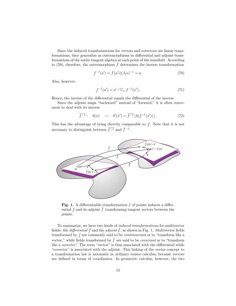
Fig. 1. A differentiable transformation f of points induces a differ-ential f and its adjoint f transforming tangent vectors between thepoints.

To summarize, we have two kinds of induced transformations for multivectorfields: the differential f and the adjoint f , as shown in Fig. 1. Multivector fieldstransformed by f are commonly said to be contravariant or to “transform like avector,” while fields transformed by f are said to be covariant or to “transformlike a covector.” The term “vector” is thus associated with the differential while“covector” is associated with the adjoint. This linking of the vector concept toa transformation law is axiomatic in ordinary tensor calculus, because vectorsare defined in terms of coordinates. In geometric calculus, however, the two

15

concepts are separate, because the algebraic concept of vector is determinedby the axioms of geometric algebra without reference to any coordinates ortransformations.

As we have just seen, one way to assign a transformation law to a vector ora vector field is by relating it to differentiation. Another way is by the rule ofdirect substitution: A field F = F (x) is transformed to F (f−1(x′)) = F ′(x′) or,equivalently, to

F ′(x′) ≡ F ′(f(x)) = F (x) . (73)

Thus, the values of the field are unchanged — although they are associated withdifferent points by changing the functional form of the field.

Directional derivatives of the two different functions in (73) are related bythe chain rule:

a ·F = a ·xF ′(f(x)) = (a ·xf(x)) ·x′F ′(x′) = f(a) ·′F ′ = a′ ·′

F ′ .

(74)

The chain rule is more simply expressed as an operator identity

a · = a · f (′) = f(a) ·′

= a′ ·′. (75)

Differentiation with ∂a yields the general transformation law for the vectorderivative:

= f (′) or ′

= f −1() . (76)

This is the chain rule for the vector derivative, the most basic form of the chainrule for differentiation on vector manifolds. All properties of induced transfor-mations are essentially implications of this rule, including the transformationlaw for the differential, as (75) shows.

Sometimes it is convenient to use a subscript notation for the differential:

fa ≡ f(a) = a ·f. (77)

Then the second differential of the transformation (63) can be written

fab ≡ b · a ·f = b ·[f(a)] − [f(b ·a)] , (78)

and we note that

fab = fba. (79)

This symmetry is equivalent to the fact that the adjoint function has vanishingcurl. Thus, using = ∂aa · we prove

∧ f (a′) = ∂b ∧ fb(a′) = ∂b ∧ ∂cfcb · a′ = ∧f · a′ = 0 . (80)

16

The transformation rule for the curl of a covector field a = f (a′) is therefore

∧ a = ∧ f (a′) = f (′ ∧ a′) . (81)

To extend this to multivector fields of any grade, note that the differential of anoutermorphism is not itself an outermorphism; rather it satisfies the “productrule”

fb(A′ ∧ B′) = fb(A′) ∧ f (B′) + f (A′) ∧ fb(B′) . (82)

Therefore, it follows from (80) that the curl of the adjoint outermorphism van-ishes, and (81) generalizes to

∧ A = f (′ ∧ A′) or ′ ∧ A′ = f −1(∧ A) , (83)

where A = f (A′). Thus, the adjoint outermorphism of the curl is the curl of anoutermorphism.

The transformation rule for the divergence is more complex, but it can bederived from that of the curl by exploiting the duality of inner and outer prod-ucts

a ∧ (Ai) = (a · A)i (84)

and the transformation law (58) relating them. Thus,

f (′ ∧ (A′i)) = f [ (′ · A′)i ] = f−1(′ · A′)f (i) .

Then, using (83) and (66) we obtain

∧ f (A′i) = ∧ [ f−1(A′)f (i) ] = · (JfA)i ,

where A′ = f(A). For the divergence, therefore, we have the transformationrule

′ · A′ = ′ · f(A) = Jf−1 f [ · (JfA) ] = f [ · A + ( lnJf ) · A ] , (85)

This formula can be separated into two parts:

′ · f (A) = f [ ( ln Jf ) · A ] = (′ln Jf ) · f(A) , (86)

′ · f(A) = f( · A) . (87)

The whole can be recovered from the parts by using the following generalizationof (75) (which can also be derived from (58)):

f(A) ·′= f(A ·) . (88)

17

IV. Induced Geometry on Flat Spacetime

Every real entity has a definite location in space and time — this is the funda-mental criterion for existence assumed by every scientific theory. In Einstein’srelativity theories the spacetime of real physical entities is a 4-dimensional con-tinuum modeled mathematically by a 4D differentiable manifold M4. The stan-dard formulation of general relativity (GR) employs a curved space model ofspacetime, which places points and vector fields in different spaces. In contrast,our flat space model of spacetime identifies the spacetime manifold M4 withthe Minkowski vector space of special relativity. A spacetime map describes aspatiotemporal partial ordering of physical events by representing the events aspoints (vectors) in M4 = x. All other properties of physical entities are rep-resented by fields on spacetime with values in the tangent algebra V4(x) and thegeometric algebra G(V4) that it generates. For this reason it is worthwhile tomaintain a distinction between V4 and M4 even though they are algebraicallyidentical vector spaces.

To incorporate gravity into flat space theory we represent metrical relationsamong events by fields in V4 rather than intrinsic properties of M4 as in curvedspace theory. The following subsections explain how to do that in a systematicway that is easily compared to Einstein’s curved space theory.

A. Displacement Gauge Invariance

A given ordering of events can be represented by a map in many differentways, just as the surface of the earth can be represented by Mercator projection,stereographic projection or many other equivalent maps. As the physical worldis independent of the way we construct our maps, we seek a physical theorywhich is equally independent. The Cambridge group has formulated this ideaas a new kind of gauge principle, which can be expressed as follows:

Displacement Gauge Principle (DGP): The equations of physicsmust be invariant under arbitrary smooth remappings of events ontospacetime.

To give this principle a precise mathematical formulation, from here on weinterpret the transformation (63) as a smooth remapping of flat spacetime M4

onto itself. It will be convenient to cast the direct substitution transformation(73) of a field F = F (x) in the alternative form

F ′(x) ≡ F (x′) = F (f(x)) . (89)

This simple transformation law, assumed to hold for all physical fields and fieldequations, is the mathematical formulation of the DGP. The descriptive term“displacement” is justified by the fact that (89) describes displacement of thefield from point x to point x′ without changing its values. The DGP shouldbe recognized as a vast generalization of “translational invariance” in specialrelativity, so it has a comparable physical interpretation. Accordingly, the DGPcan be interpreted as asserting that “spacetime is globally homogeneous.” In

18

other words, with respect to the equations of physics all spacetime points areequivalent. Thus, the DGP has implications for measurement, as it establishesa means for comparing field configurations at different places and times.

The Cambridge group had the brilliant insight that enforcement of the trans-formation law (89) requires introduction of a new physical field that can be iden-tified with the gravitational field. Properties of this field, called the gauge fieldor gauge tensor, derive from the transformation laws of the preceding section.The most essential step is defining a gauge invariant derivative. To that end,consider a gauge invariant scalar field φ = φ(x) transformed by (89); accordingto (76) the transformation of its gradient is given by

φ′(x) = φ(f(x)) = f [′φ(x′)] . (90)

To make this equation gauge invariant, we introduce an invertible tensor fieldh defined on covectors so that

h′[(φ′(x)] = h[(′φ(x′)] . (91)

Comparison with (90) shows that h must be a linear operator on covectors withthe transformation law

h′ = hf −1 . (92)

More explicitly, when operating on a covector b = φ the rule is

h′(b; x) = h(f −1(b;x);x′) . (93)

We usually suppress the position dependence and write

h′(b) = h(f −1(b)) . (94)

Applying this rule to the vector derivative with its transformation rule (76),we can define a position gauge invariant derivative by

≡ h() . (95)

The symbol is a convenient abuse of notation to remind us that the linearoperator h is involved in its definition.

From the operator we obtain a position gauge invariant directional deriva-tive

a · = a · h() = (ha) · , (96)

where h is the adjoint of h and a is a “free vector,” which is to say that it canbe regarded as constant or as a vector transforming by the direct substitutionrule (89). This is clarified by a specific example.

Let x = x(τ) be a timelike curve representing a particle history. Accordingto (64), the diffeomorphism (63) induces the transformation

x =dx

dτ→ x′ = f(x.) . (97)

19

Thus the description of particle velocity by x. is “contravariant” under spacetime

diffeomorphisms. Comparing (62) with (96), it is evident that an “invariant”velocity vector v = v(x(τ)) can be introduced by writing

x = h(v) , (98)

where h obeys the adjoint of the “gauge transformation” rule (92), that is

f−1 h′ = h or h′ = f h . (99)

Accordingly, (97) implies that

x′ = h′(v) , (100)

where v has the same value as in (98), but it is taken as a function of x′(τ)instead of x(τ). To distinguish the x from the invariant velocity

v = h−1(x) = h′−1(x′) , (101)

one could refer to x as the map velocity. Otherwise the term “velocity” desig-nates v. The invariant normalization

v2 = 1 (102)

fixes the scale on the parameter τ , which can therefore be interpreted as propertime.

For any field F = F (x(τ)) defined on a particle history x(τ), the chain rulegives the operator relation

d

dτ= x · = h(v) · = v · h() = v · , (103)

so that

dF

dτ= v ·F . (104)

For F (x) = x, this gives

dx

dτ= v ·x = (hv) ·x = hv , (105)

recovering (98).Since h and h are mutually determined, we can refer to either as the “gauge

tensor” or, simply, the “gauge” on spacetime. Actually, the term “gauge” ismore appropriate here than elsewhere in physics, because h does indeed deter-mine the “gauging” of a metric on spacetime. To see that, use (97) in (101)to derive the following expression for the invariant line element on a timelikeparticle history:

dτ2 = [ h−1(dx) ]2 = dx · g(dx) (106)

20

where

g = h−1 h−1 (107)

is a symmetric metric tensor. This formulation suggests that gauge is a morefundamental geometric entity than metric, and that view is confirmed by devel-opments below. Einstein has taught us to interpret the metric tensor physicallyas a gravitational potential, making it easy and natural to transfer this inter-pretation to the gauge tensor. Some readers will recognize h as equivalent to a“tetrad field,” which has been proposed before to represent gravitational fieldson flat spacetime [16]. However, the spacetime calculus makes all the differencein turning the tetrad into a practical tool.

To verify that (106) is equivalent to the standard invariant line element ingeneral relativity, coordinates must be introduced. Let x = x(x0, x1, x2, x3)be a parametrization of the points, in some spacetime region, by an arbitraryset of coordinates xµ. Partial derivatives then give tangent vectors to thecoordinate curves ∂µx, which, in direct analogy to (98) and (101), determine aset of displacement gauge invariant vector fields gµ according to the equation

eµ ≡ ∂µx =∂x

∂xµ= h(gµ) , (108)

or, equivalently, by

gµ = h−1(eµ) . (109)

The components for this coordinate system are then given by

gµν = gµ · gν = eµ · g(eν) . (110)

Therefore, with dx = dxµeµ, the line element (106) can be put in the form

dτ2 = gµνdxµdxν , (111)

which is familiar from the tensor formulation of GR.To complete the introduction of coordinates into the flat space gauge theory,

we introduce coordinate functions xµ = xµ(x) and the coordinate frame vectors

eµ = xµ (112)

reciprocal to the frame eµ defined by (108); whence

eµ · eν = eµ ·xν = ∂µxν = δνµ . (113)

The displacement gauge invariant frame gµ reciprocal to (109) is then givenby

gµ = h(eµ) = xµ . (114)

21

So the gauge invariant derivative is given by

= h() = gµ∂µ . (115)

The flat space and curved space theories can now be compared throughtheir use of coordinates. The vector fields gµ encode all the information in themetric tensor gµν = gµ · gν of GR, as is evident in (110). However, equations(111) and (114) decouple coordinate dependence of the metric, expressed byeµ = ∂µx, from the physical dependence, expressed by the gauge tensor h or itsadjointh. In other words, the remapping of events in spacetime is completelydecoupled from changes in coordinates in the gauge theory, whereas the curvedspace theory has no means to separate passive coordinate changes from shiftsin physical configurations. This crucial fact is the reason why the DisplacementGauge Principle has physical consequences, whereas Einstein’s general relativityprinciple does not.

The precise theoretical status of Einstein’s general relativity principle (GRP),also known as the general covariance principle, has been a matter of perennialconfusion and dispute that some say originated in confusion on Einstein’s part[17]. One of Einstein’s main motivations in formulating it was epistemologi-cal: to extend the special relativity principle, requiring physical equivalence ofall inertial frames, to physical equivalence of arbitrary reference frames. Heformulated the GRP as requiring covariance of the equations of physics un-der the group of arbitrary coordinate transformations (also known as generalcovariance). While acknowledging criticisms that the requirement of generalcovariance is devoid of physical content, Einstein continued to believe in theGRP as a cornerstone of his gravitation theory.

Gauge theory throws new light on the GRP, which may be regarded as vin-dicating Einstein’s obstinate stance. The problem with Einstein’s GRP is thatit is not a true symmetry principle [17]. For a transformation group to be aphysical symmetry group, there must be a well defined “geometric object” thatthe group leaves invariant. Thus the “displacement group” of the DGP is a sym-metry group, because it leaves the flat spacetime background invariant. That iswhy it can have the physical consequences described above. There is no com-parable symmetry group for curved spacetime, because each mapping producesa new spacetime, so there is no geometric object to be left invariant. Moreover,general covariance does not discriminate between passive coordinate transfor-mations and active physical transformations. Those distinctions are generallymade on an ad hoc basis in applications. The intuitive idea of physically equiv-alent situations was surely at the back of Einstein’s mind when he insisted onheuristic significance of the GPR over the objections of Kretschmann and otherson its lack of physical content. I submit that the DGP provides, at last, a pre-cise mathematical formulation for the kind of GRP that Einstein was lookingfor. Once again I am impressed by Einstein’s profound physical insight, whichserved him so well in assessing the significance of mathematical equations inphysics. Of course, his conclusions depended critically on the mathematics athis disposal, and displacement gauge theory was not an option available to him.

22

B. Rotation Gauge Covariance

Gauge theory gravity requires one other gauge principle, which we formulateas follows:

Rotation Gauge Principle (RGP): The equations of physics mustbe covariant under local Lorentz rotations.

Generalizing the treatment in Section IIIB, we characterize a local Lorentz ro-tation by a position dependent rotor field L = L(x) with LL = 1. This enablesus to define two kinds of covariant fields, a multivector field M = M(x) and aspinor field ψ = ψ(x), with respective transformation laws:

L : M → M ′ = L M ≡ LML , (116)

L : ψ → ψ′ = Lψ . (117)

Spinors and multivectors are related by the fact that the spinor field deter-mines a frame of multivector observables ψγµψ, where γµ is the standardorthonormal frame of constant vectors introduced in equation (1). Frame inde-pendence of the gauge tensor is ensured by (116), which implies that the gaugetensor satisfies the operator transformation law

L : h → h′ = L h . (118)

From (114) it follows that this transformation leaves the metric tensor gµν =gµ · gν invariant.

To construct field equations that satisfy the RGP, we define a “gauge co-variant derivative” or coderivative operator D as follows. With respect to acoordinate frame gµ = h−1(eµ), components Dµ = gµ · D of the coderivativeare defined for spinors and multivectors respectively by

Dµψ = (∂µ + 12ωµ)ψ , (119)

DµM = ∂µM + ωµ × M , (120)

where the connexion for the derivative

ωµ = ω(gµ) (121)

is a bivector-valued tensor evaluated on the frame gµ. From Section IA,we know that the bivector property of ωµ implies that ωµ × M is “gradepreserving.” Hence Dµ is a “scalar differential operator” in the sense thatgrade(DµM) =grade(M). Note that Dµ is not grade-preserving on the spinorin (119).

To ensure the covariant transformations for the derivatives

L : Dµψ → L(Dµψ) = D′µψ′ = (∂µ + 1

2ω′µ)ψ′ , (122)

23

L : DµM → L (DµM) = D′µM ′ = ∂µM ′ + ω′

µ × M ′ , (123)

the connexion must obey the familiar gauge theory transformation law

ωµ = → ω′µ = LωµL − 2(∂µL)L , (124)

where it should be noted that the operator ∂µ = gµ · is rotation gauge in-variant. The full vector coderivative D can now be defined by the operatorequation

D = gµDµ , (125)

for which gauge covariance follows from (118) and the definition of Dµ. SinceDµ preserves the grade of M in (120), the coderivative is a vector differentialoperator, so we can decompose it in the same way that we decomposed thevector derivative into divergence and curl in equation (31). Thus, for anarbitrary covariant multivector field M = M(x), we can write

DM = D · M + D ∧ M , (126)

where D · M and D ∧ M are respectively the codivergence and the cocurl.Combining (118) with (92), we see that the most general transformation of

the gauge tensor is given by

h′ = L hf −1, h′ = f hL . (127)

In other words, every gauge transformation on spacetime is a combination ofdisplacement and local rotation. This operator equation enables us to turn anymultivector field on spacetime into a gauge covariant field, as shown explicitlyin the next section for the electromagnetic field. Finally, it should be notedthat all the above rotation covariant quantities, including the connexion ωµ, aredisplacement gauge invariant as well.

In special relativity, Lorentz transformations are passive rotations express-ing equivalence of physics with respect to different inertial reference frames.Here, however, covariance under active rotations expresses local physical equiv-alence of different directions in spacetime. In other words, the rotation gaugeprinciple asserts that spacetime is locally isotropic. Thus, “passive equivalence”is an equivalence of observers, while “active equivalence” is an equivalence ofstates. This distinction generalizes to the physical interpretation of any sym-metry group principle: Active transformations relate equivalent physical states;passive transformations relate equivalent observers.

To establish the connection of GTG to GR, we need to relate the coderivativeto the usual covariant derivative in GR. Like the directional derivative ∂µ =gµ ·, the directional coderivative Dµ = gµ · D is a “scalar differential operator”that maps vectors into vectors. Accordingly, we can write

Dµgν = Lαµνgα , (128)

24

which merely expresses the derivative as a linear combination of basis vectors.This defines the so-called coefficients of connexion Lα

µν for the frame gν. Bydifferentiating gα · gν = δα

ν , we find the complementary equation

Dµgα = −Lαµνgν . (129)

When the coefficients of connexion are known functions, the coderivative of anymultivector field is determined.

Thus, for any vector field a = aνgν we have

Dµa = (Dµaν)gν + aν(Dµgν).

Then, since the aν are scalars, we get

Dµa = (∂µaα + aνLαµν)gα . (130)

Note that the coefficient in parenthesis on the right is the standard expressionfor a “covariant derivative” in tensor calculus.

Further properties of the connection are obtained by contracting (129) withgµ to obtain

D ∧ gα = gν ∧ gµLαµν . (131)

This bivector-valued quantity is called torsion. In the Riemannian geometry ofGR torsion vanishes, so we restrict our attention to that case. Considering theantisymmetry of the outer product on the right side of (131), we see that thetorsion vanishes if and only if

Lµαβ = Lµ

βα . (132)

This can be related to the metric tensor by considering

Dµgαβ = ∂µgαβ = (Dµgα) · gβ + gα · (Dµgβ) ,

whence

∂µgαβ = gανLνµβ + gβνLν

µα . (133)

Combining three copies of this equation with permuted free indices, we solve for

Lµαβ = 1

2gµν(∂αgβν + ∂βgαν − ∂νgαβ) . (134)

This is the classical Christoffel formula for a Riemannian connexion, so the de-sired relation of the coderivative to the covariant derivative in GR is established.

C. Curvature and Coderivative

In standard tensor analysis the curvature tensor is obtained from the commu-tator of covariant derivatives. Likewise, we obtain it here from the commutatorof coderivatives. Differentiating (129) we get

[Dµ, Dν ]gα = Rαµνβgβ , (135)

25

where the operator commutator has the usual definition

[Dµ, Dν ] ≡ DµDν − DνDµ , (136)

and

Rαµνβ = ∂µLα

νβ − ∂νLαµβ + Lα

νσLσµβ − Lα

µσLσνβ , (137)

is the usual tensor expression for the Riemannian curvature of the manifold.This suffices to establish mathematical equivalence of our flat space gauge theoryto the standard tensor formulation of Riemannian geometry and hence to GR.Now we can confidently turn to the full gauge theory treatment of curvatureand gravitation to see what advantages it has over standard GR.

The commutator of coderivatives defined by (121) gives us

[Dµ, Dν ]M = R(gµ ∧ gν) × M , (138)

where

R(gµ ∧ gν) = ∂µων − ∂νωµ + ωµ × ων

= Dµων − Dνωµ − ωµ × ων ≡ ωµν

(139)

is the curvature tensor expressed as a bivector-valued function of a bivectorvariable. This is the fundamental form for curvature in GTG. It follows from(123) that the curvature bivector has the covariance property

L : R(gµ ∧ gν) → R′(g′µ ∧ g′ν) = L R(L (gµ ∧ gν)), (140)

where L = L−1.For the gravity field variables gµ, equations (138) and (135) give us

[Dµ, Dν ]gα = ωµν · gα = Rαµνβ gβ ; (141)

whence

Rαµνβ = ωµν · (gα ∧ gβ). (142)

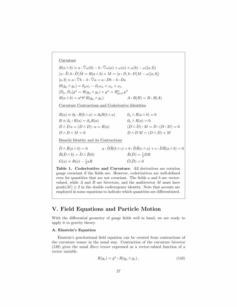
Coordinate frame fields gµ and gµ have been used to introduce thecoderivative and curvature in order to make connection with the standard ten-sor formalism as direct as possible. However, the vector coderivative and thecurvature bivector can be defined and all their properties can be derived ina completely coordinate-free way. Derivations are given in Appendix B, andresults are summarized in Table 1.

26

Curvature

R(a ∧ b) ≡ a ·ω(b) − b ·ω(a) + ω(a) × ω(b) − ω([a, b])

[a · D, b · D ]M = R(a ∧ b) × M = [a · D, b · D ]M − ω([a, b])

[a, b] ≡ a ·b − b ·a = a · Db − b · Da

R(gµ ∧ gν) = ∂µων − ∂νωµ + ωµ × ων

[Dµ, Dν ]gα = R(gµ ∧ gν) × gα = Rαµνβ gβ

R(a ∧ b) = aµbνR(gµ ∧ gν) A · R(B) = B · R(A)

Curvature Contractions and Coderivative Identities

R(a) ≡ ∂b · R(b ∧ a) = ∂bR(b ∧ a) ∂a ∧ R(a ∧ b) = 0

R ≡ ∂a · R(a) = ∂aR(a) ∂a ∧ R(a) = 0

D ∧ D a = (D ∧ D) · a = R(a) (D ∧ D) · M = D · (D · M) = 0

D ∧ D ∧ M = 0 D ∧ D M = (D ∧ D) × M

Bianchi Identity and its Contractions

D ∧ R(a ∧ b) = 0 a · DR(b ∧ c) + b · DR(c ∧ a) + c · DR(a ∧ b) = 0

R(D ∧ b) = D ∧ R(b) R(D) = 12DR

G(a) ≡ R(a) − 12aR G(D) = 0

Table 1. Coderivative and Curvature. All derivatives are rotationgauge covariant if the fields are. However, coderivatives are well-definedeven for quantities that are not covariant. The fields a and b are vector-valued, while A and B are bivectors, and the multivector M must havegrade(M) ≥ 2 in the double codivergence identity. Note that accents areemployed in some equations to indicate which quantities are differentiated.

V. Field Equations and Particle Motion

With the differential geometry of gauge fields well in hand, we are ready toapply it to gravity theory.

A. Einstein’s Equation

Einstein’s gravitational field equation can be created from contractions ofthe curvature tensor in the usual way. Contraction of the curvature bivector(139) gives the usual Ricci tensor expressed as a vector-valued function of avector variable.

R(gν) = gµ · R(gµ ∧ gν) , (143)

27

With help from the identity (13), a second contraction gives the usual scalarcurvature

R ≡ gν · R(gν) = (gν ∧ gµ) · R(gµ ∧ gν) . (144)

The gravitational field equation can thus be written in the form

G(gν) ≡ R(gν) − 12gν R = κT (gν) , (145)

where κ = 8π in “natural units” with the gravitational constant set equal tounity. The vector-valued function of a vector variable G(a) is Einstein’s tensor,and its source T (a) is the total energy-momentum tensor for material particlesand non-gravitational fields. Of course, decomposition into tensor componentsGµν = gµ · G(gν) and Tµν = gµ · T (gν) yields Einstein’s equation in its standardtensor component form.

The spacetime algebra reviewed in Section I enables us to express Einstein’stensor Gβ = G(gβ) in the new unitary form:

Gβ = 12 (gβ ∧ gµ ∧ gν) · ωµν = 1

2 (gβ ∧ ωµν) · (gµ ∧ gν) . (146)

The last equality is a consequence of the well-known symmetry of the curvaturetensor,

(gα ∧ gβ) · R(gµ ∧ gν) = (gµ ∧ gν) · R(gα ∧ gβ) . (147)

Identities (12) and (13) can be used to expand the inner product in (146) to get

Gβ = gµ · ωµνgνβ − 12gβ(gν ∧ gµ) · ωµν , (148)

which will be recognized as equivalent to the standard form (145) for the Einsteintensor. Thus, expansion of the inner product has split the “unitary” Einsteintensor into two parts. Let us refer to this as the Ricci split of the Einsteintensor.

As is well known, Einstein originally chose the particular combination ofRicci tensor and scalar curvature in (145) because, as shown in Appendix B andTable 1, its codivergence G(D) vanishes in consequence of the Bianchi identity.Using Dµ(ggµ) = 0 from appendix A, we can write this version of the Bianchiidentity in the form

Dµ[gG(gµ)] = gG(D) = 0 . (149)

It follows, then, from Einstein’s field equation (145) that

Dµ[gT (gµ)] = gT (D) = 0 . (150)

Initially, Einstein wanted to interpret this as a general energy-momentum con-servation law. However, that interpretation is not so straightforward, because atrue conservation law requires vanishing of an ordinary divergence rather thana codivergence. Instead, we shall see in Section VC that (150) determines the

28

equation of motion for matter. Then in Section VII we see that an alternativeto the Ricci split is more suitable for deriving the general energy-momentumconservation law that Einstein wanted.

B. Electrodynamics with Gravity

GTG differs from GR in providing explicit equations for the influence ofgravity on physical fields. This is best illustrated by electrodynamics. Maxwell’sequation F = J with F = ∧A is not gravitation gauge covariant. To makethe vector field A gauge covariant and incorporate the effect of gravity, we simplywrite [15]

A = h(A) , (151)

and gauge covariance is assured by (127). In fact, the influence of gravity onthe electromagnetic field is fully characterized by the gauge tensor h.

Now applying (240) from Appendix A to (151), we immediately obtain agauge covariant expression for the electromagnetic field strength:

F = h(F ) = D ∧ A = h(∧ A ) . (152)

Similarly, applying the cocurl again and using Table 1, we obtain

D ∧ F = D ∧ D ∧ A = h(∧∧ A ) = 0 . (153)

Thus, Maxwell’s equation ∧ F = 0 applies irrespective of the gravitationalfield. Now it is obvious that the gauge covariant form of Maxwell’s equationmust be

D F = D · F + D ∧ F = J . (154)

From the vector part of this equation, we have, using the double codivergenceidentity in Table 1,

D · (D · F ) = 0 = D · J , (155)

A little more analysis is needed to relate the right side of this equation to thestandard charge current conservation law.

Explicit dependence of the codivergence D · F on the gauge tensor can bederived from (152) by exploiting duality. The derivation is essentially the sameas that for (85) and yields the result

D · F = hh−1[ · (h−1 h(F ))] , (156)

where h ≡ det(h). For the vector field J the result is a scalar, and we obtainthe simpler equation

D · J = h · (h−1 h(J )) , (157)

29

so comparison with (155) identifies J = h−1 h(J ) with the conserved chargecurrent. Combining this with (156), we can write D · F = J in the equivalentform

· (h−1 hh(F )) = J . (158)

This enables us to interpret the operator h−1 hh = h−1 g−1 as a kind of dielectrictensor or generalized index of refraction for the “gravitational medium” [18]. Ofcourse, equation (158) can be used to compute refraction of light by the sun,with a result in agreement with alternative GR calculations.

The standard Maxwell energy-momentum tensor (as given in GA2) is easilygeneralized to the gauge covariant form:

TEM (a) = −12F aF (159)

Using (153) to compute its coderivative , we obtain

TEM (D) = − 12 (F DF + F DF ) = 1

2 (J F − F J ) . (160)

In other words,

Dµ[gTEM (gµ)] = gTEM (D) = gF · J . (161)

One way to assure mutual consistency of Einstein’s field equation with Maxwell’sequation is to derive them from a common Lagrangian. This has been doneby the Cambridge group in a novel way with GC, and the method has beenextended to spinor fields with provocative new results. The reader is referredto the literature for details [2].

C. Equations of Motion from Einstein’s Equation

In classical electrodynamics Maxwell’s field equation and Lorentz’s equationof motion for a charged particle must be postulated separately. It came asquite a surprise, therefore, to discover that in GR the equation of motion fora material particle can be derived from Einstein’s field equation, provided it isassumed to hold everywhere, including at any singularities in the gravitationalfield. This discovery was made independently by several people, though mostof the credit is unfairly given to Einstein [19]. Here we sketch essential elementsin one especially simple approach to deriving equations of motion to illustrateadvantages of using GA. The form of the equation of motion is determined bythe form of the energy-momentum tensor. The idea is to describe a localizedmaterial system as a point particle by a multipole expansion of the mass distri-bution. Then the problem is to reformulate the result as a differential equationfor the particle.

We consider only the simplest case of a structureless point particle. For afluid of non-interacting material particles, the energy-momentum tensor can beput in the form

TM (a) = mρ(a · v)v, (162)

30

where ρ is the proper particle density, v is the proper particle velocity and m isthe mass per particle. Its codivergence is

TM (D) = TM () + ωµ · T (gµ) = mvD · (ρv) + mρv · Dv. (163)

As shown in (157) for a charge current, the codivergence D · (ρv) can be ex-pressed as a true divergence, so its vanishing expresses particle conservation,which we assume holds here. For a single particle, ρ is a δ-function on the par-ticle history, and it can be eliminated by integration, but we don’t need thatstep here.

For a charged particle the total energy-momentum tensor is

T (a) = TM (a) + TEM (a) = mρa · vv − 12F aF . (164)

According to (161) and (163), its codivergence is

Dµ[g(TM (gµ) + TEM (gµ)] = gρmv · Dv + gJ · F . (165)

For a particle with charge q the current density is J = qρv, so the vanishing of(165) gives us

mv · Dv − qF · v = 0. (166)

This has the desired form for the equation of motion of a point charge. ForF = 0 it reduces to the geodesic equation, as described in the next Section.

The electromagnetic field in (166) can be expressed as a sum F = F self +F ext, where F self is the particle’s own field and F ext is the field of other parti-cles. Evaluated on the particle history, F self describes reaction of the particleto radiation it emits. This process has been much studied in the literature [19],but the analysis is too complicated to discuss here. If we neglect radiation, wecan write F = F ext in (166), and qF · v is the usual Lorentz force on a “testcharge.”

D. Particle Motion and Parallel Transfer

The equation for a particle history x = x(τ) generated by a timelike velocityv = v(x(τ)) in the presence of an “ambient” gauge tensor h is x

. = h(v). For anycovariant multivector field M = M(x(τ)), eqn. (120) gives us the directionalcoderivative

v · DM =d

dτM + ω(v) × M , (167)

where the gauge invariant proper time derivative is given by (104). Obviously,all this applies to arbitrary differentiable curves in spacetime if the requirementthat v be timelike is dropped.

The equation for a geodesic can now be written

v · Dv = v. + ω(v) · v = 0 (168)

31

With ω(v) specified by the “ambient geometry,” this equation can be integratedfor v = h−1(x.) and then a second integration gives the geodesic curve x(τ).The solution is facilitated by noting that (168) implies

v · v. = 1

2

dv2

dτ= v · ω(v) · v = ω(v) · (v ∧ v) = 0 . (169)

Therefore v2 is constant on the curve and, as noted in GA2, the value of v atany point on the curve can be obtained from a timelike reference value v0 by aLorentz rotation. Thus,

v = R v0 = Rv0R , (170)

where R = R(x(τ)) is a rotor field on the curve satisfying the differential equa-tion

v · DR =dR

dτ+ 1

2ω(v)R = 0 . (171)

This is equivalent to the spinor derivative (119), so the rotor R can be regardedas a special kind of spinor.

More generally, the parallel transport of any fixed multivector M0 to a fieldM = M(x(τ)) defined on the whole curve is given by

M = R M0 = RM0R . (172)

Of course, it satisfies the differential equation

v · DM = M + ω(v) × M = 0 . (173)

The formal similarity of this formulation for parallel transport to a directionalgauge transformation is obvious, but the two should not be confused.

With the spinor coderivative defined by (171) (and not necessarily vanish-ing), we can rewrite (167) as an operator equation

v · D = Rd

dτR, (174)

or equivalently, as

Rv · D = v ·R =d

dτR . (175)

This shows that a coderivative can be locally transformed to an ordinary deriva-tive by a suitable gauge transformation.

According to (166), for a particle with unit mass and charge q in an elec-tromagnetic field F = h(F ) = D ∧ A = h(∧ A), the geodesic equation (168)generalizes to

v. = v · ω(v) + qF · v , (176)

32

The first term on the right can be interpreted as a “gravitational force,” thoughthe standard GR interpretation regards it as part of “force-free” geodesic mo-tion. From (246) and (242) in Appendix A, we see that v · (v · H) = (v∧v) · H =0, so

v · ω(v) = v · H(v) = −v · h [ ∧ h−1(v)] , (177)

where the accent indicates which quantity is differentiated. Thus, the “gravi-tational force” is determined by the bivector-valued function H(v), and we canwrite

v · H(v) + qF · v = h[ ( ∧ h−1(v) + ∧ A) ] · h−1(x.)

= h[ ( ∧ h−1(v) + ∧ A) · x. ].

(178)

Finally, on expanding the last term and introducing the metric tensor g definedby (107), we can put the equation of motion (176) in the form

d

dτ[ g(x.) + qA] = [ 1

2x. · g(x.) + qA · x

. ] . (179)

Except for the presence of the metric tensor g, this is identical to the equationof motion for a point charge in Special Relativity, so we can use familiar tech-niques from that domain to solve it (details in Section VII). Ignoring the vectorpotential and solving for

..x , it can be put in the form

..x = g−1

[12x

. · g(x.) − g(x.)] . (180)

This is equivalent to the standard formulation for the geodesic equation in termsof the “Christoffel connection.” Note how the metric tensor appears when theequation of motion is formulated in terms of a spacetime map rather than incovariant form.

E. Gravitational Precession and Dirac Equation

The solution of equation (171) gives more than the velocity. In perfect anal-ogy with the treatment of electromagnetic spin precession in GA2, it gives usa general method for evaluating gravitational effects on the motion and preces-sion of a spacecraft or satellite, and thus a means for testing gravitation theory.To the particle worldline we attach a (comoving orthonormal frame) or mobileeµ = eµ(x(τ)) = eµ(τ);µ = 0, 1, 2, 3. The mobile is tied to the velocity byrequiring v = e0. Rotation of the mobile with respect to a fixed orthonormalframe γµ is described by

eµ = R γµR , (181)

where R = R(x(τ)) is a unimodular rotor. This has the same form as equation(24) for a mobile in flat spacetime because the background spacetime is flat.

33

Applying (167) to (181) we obtain the coderivative of the mobile:

v · Deµ = eµ + ω(v) · eµ . (182)

The coderivative here includes a gauge invariant description of gravitationalforces on the mobile. In accordance with (21) and (23), effects of any nongrav-itational forces can be incorporated by writing

v · Deµ = eµ + ω(v) · eµ = Ω · eµ , (183)

where Ω = Ω(x) is a bivector such as an external electromagnetic field actingon the mobile. The four equations (183) include the equation of motion

dv

dτ= (Ω − ω(v)) · v (184)

for the particle, and are equivalent to the single rotor equation

dR

dτ= 1

2 (Ω − ω(v))R . (185)

For Ω = 0 the particle equation becomes the equation for a geodesic, and therotor equation describes parallel transfer of the mobile along the geodesic. Thisequation has been applied to gravitational precession in [20], so there is no needto elaborate here.

Our rotor treatment of classical gravitational precession generalizes directlyto gravitational interactions in quantum mechanics. We saw in (40) that a realDirac spinor field ψ = ψ(x) determines an orthonormal frame of vector fieldseµ = eµ(x) = RγµR . Generalization of the real Dirac equation (38) to includegravitational interaction is obtained simply by replacing the partial derivative∂µ by the coderivative Dµ defined by equation (119). Thus, we obtain

gµDµψγ2γ1h = gµ(∂µ + 12ωµ)ψγ2γ1h = eA ψ + mψγ0 , (186)

where A = h(A) is the gauge covariant vector potential. This is equivalent tothe standard matrix form of the Dirac equation with gravitational interaction,but it is obviously much simpler in formulation and application. Comparisonof the spinor coderivative (119) with the rotor coderivative (185) tells us imme-diately that gravitational effects on electron motion, including spin precession,are exactly the same as on classical rigid body motion. The Cambridge grouphas studied solutions of the real Dirac equation (186) in the field of a black holeextensively [21].

VI. Solutions of Einstein’s Equation

Though GC facilitates curvature calculations, the nonlinearity of Einstein’sequation still makes it difficult to solve. Gauge theory gravity introduces simpli-fications both in calculation and physical interpretation by cleanly separating

34

the functional form of the gauge tensor from arbitrary choices of coordinatesystem. Using results in the Appendices and Table 1, gravitational curvaturecan be calculated from a given gauge tensor by the straightforward sequence ofsteps:

h(a) → ∧ h−1

(a) → ω(a) → R(a ∧ b) . (187)

To solve Einstein’s equation for a given physical situation, symmetry consider-ations are used to restrict the functional form of the gauge tensor, from whicha functional form for the curvature tensor is derived by (187). This, in turn, isused to simplify the form of Einstein’s tensor and reduce Einstein’s equation tosolvable form. Finally, gauge freedom is used to analyze alternative forms forthe solution and ascertain the simplest for a given application. Details, framedsomewhat differently, are given in [2] and other publications by the Cambridgegroup, so they need not be repeated here. We confine our attention to a reviewof results that showcase advantages of the GC formulation and analysis.

A. Static Black Hole

The most fundamental result of GR is the gravitational field of a point particleat rest called a black hole. To construct a spacetime map of this field and themotion of particles within it, we represent the velocity of the hole by the constantunit vector γ0 and locate the origin on its history. As explained in GA2, thisdefines a preferred reference frame and a spacetime split of each spacetime pointx into designation by a time t = x · γ0 and a relative position vector x = x∧ γ0,and a split of the vector derivative ∂t = γ0· and ∇ = γ0 ∧, as expressed by

xγ0 = t + x, γ0 = ∂t + ∇. (188)

It will also be convenient to write r = |x ∧ γ0| = |x| so that x = rx, and tointroduce the unit radius vector

er = ∂rx = −r = xγ0. (189)

The Cambridge group has shown that the curvature tensor for a black holecan be written in the wonderfully compact form [2, 3]

R(B) = − M

2r3(B + 3xBx), (190)

where M is the mass of the black hole. Considering the local Lorentz rotation ofthe curvature (140), it is evident at once that the curvature tensor is invariantunder a boost in the x = erγ0 plane, as expressed by

L x = LxL = x. (191)

This simple symmetry of the curvature tensor has long remained unrecognizedin standard tensor formulations of GR.

35

Using the vector derivative identity (28), it is not difficult to verify by directcalculation that

R(b) = ∂aR(a ∧ b) = 0, (192)

so Einstein’s tensor G(a) vanishes when r = 0. As is evident in (190), thecurvature is singular at r = 0; this can be shown to arise from a delta-functionin the energy-momentum tensor:

T (a) = 4πδ3(x)(a · γ0)γ0 . (193)

This simple expression for the singularity contrasts with standard GR where theblack hole singularity is not so well defined, and it is often claimed that suchentities as “wormholes” are allowed [12]. Unfortunately for science fiction buffs,GTG rules out wormholes by requiring global solutions of Einstein’s equation,as explained below.

The standard Schwarzschild solution of Einstein’s field equation for a blackhole is equivalent to the symmetric gauge tensor

hS(a) = (α−1a · γ0 + αa ∧ γ0)γ0, α =(

1 − 2M

r

) 12

. (194)

Alternative solutions can be generated by gauge transformations that leave thecurvature (190) invariant. Allowed transformations are determined by threeparameters. One parameter is fixed by boundary conditions at infinity, a sec-ond generates displacements, and the third generates boosts defined by (191).The Cambridge group [3] has found boost-displacements that transform the“Schwarzschild gauge” (194) into a “Kerr-Schild gauge”

hKS(a) = a +M

ra · (γ0 − er)(γ0 − er), (195)

and a “Newtonian gauge”

h(a) = a − ϕ(a · γ0)er, ϕ =(

2M

r

) 12

. (196)

The former corresponds to such well-known solutions as the Eddington-Finkelsteinmetric, while the latter has hardly been noticed in the GR literature, despite itsconsiderable virtues, which we now expose. It should be noted that the Newto-nian gauge (196) is well-defined for every r = 0, while the Schwarzschild gauge(194) has a well-known singularity at r = 2M . Therefore, the former is a moregeneral solution to Einstein’s equation than the latter.

To interpret results of physical measurements in the gravitational field, wefollow the usual practice of setting up reference systems of imaginary observers.First, consider a stationary observer at a fixed distance r from the black hole,so his world line is defined by the map velocity

x. = t

.γ0, (197)

36

so x = 0. As only gauge covariant quantities are physically significant, we mustconsider the observer’s “gauge velocity” determined by (196):

v = h−1x. = t

.(γ0 + ϕer). (198)

Whence the constraint v2 = 1 implies

t.=

(1 − 2M

r

)− 12

. (199)

This tells us that the stationary observer’s clock (reading proper time τ) runsslow compared to the proper time t of the black hole. But how can we “read” aclock on the black hole? That is answered by considering a freely-falling observerwith a constant gauge velocity v = γ0 equal to that of the black hole, so hismap velocity is

x. = h−1γ0 = γ0 + ϕer, (200)

which we solve immediately for

t.= x

. · γ0, r. = −x

. · er = −ϕ = −(

2M

r

) 12

. (201)

This tells us that the clock of a freely falling observer has the same rate as theproper time of the black hole, and his velocity r

. is identical to the infall velocityin Newtonian theory. This justifies the name “Newtonian gauge” introducedabove and suggests referring to time t as “Newtonian time.”

As our discussion of observers suggests, the Newtonian gauge simplifies phys-ical interpretation and analysis of motion in the gravitational field of a pointparticle. It has the great advantage of showing precisely how GR differs fromNewtonian theory in this case. To compare with standard GR, we need the“Newtonian” gauge tensor, which from (196) is

g a = h−1 h−1a = a + ϕ(a · γ0 er + a · erγ0) − ϕ2a · γ0γ0. (202)

This determines a line element

ds2 = dx · g dx = dt2 − (dr + ϕdt)2 − r2dΩ2. (203)

This line element does not appear in any GR textbook. Only Ron Gautreauhas expounded its pedagogical benefits in a series of AJP articles [22]. All hisanalysis can be neatly reformulated in Newtonian gauge theory.

Now, to analyze the general motion of a point charge in the Newtoniangauge, we multiply equation (179) by γ0 to do a space-time split. Consideringfirst the scalar part of the split, for static fields ∂t g = 0 and ∂tA = 0 we findimmediately the constant of motion

E = ( gx. + qA) · γ0 = v · u + V , (204)

37

where V = qA · γ0 is the usual electric potential and

v · u = γ0 · gx = h−1(γ0) · h−1(x.) = t.(1 − ϕ2) − ϕr

.. (205)

We recognize this as a gauge invariant generalization of energy conservation inspecial relativity. The time derivative can be eliminated from this expressionwith the constraint

1 = v2 = (x. + ϕt.er)2 = (1 − ϕ2)t

.2 − 2t.r. − x2 . (206)

As our analysis to this point is sufficient to show how electromagnetic interac-tions can be included, let us omit them from the rest of our analysis to con-centrate on the distinctive features of the gravitational interaction. Introducingthe angular momentum (per unit mass)

L = x ∧ x = r2x ˙x (207)

so we can write

x2 = r.2 +

L2

r2(208)

with L2 = −L2, we eliminate t.

between (204) and (206) to get an equationgoverning radial motion of the particle:

E2 = (1 − ϕ2)(

1 +L2

r2

)+ r

.2. (209)

A pedagogically excellent analysis of the physical implications this equation andrelated issues in elementary black hole physics is given by Taylor and Wheeler[23]. Their treatment could be further simplified by adopting the Newtoniangauge.

To complete our analysis of motion in the Newtonian gauge, we return tothe space-time split of equation (179) to consider the bivector part, which givesus the spatial equation of motion

g = −∇ 12x

. · g(x.) , (210)

and, from (202), we get the more explicit expressions

g ≡ ( gx.) ∧ γ0 = x + ϕt

.x (211)

−∇ 12x

. · g(x.) = t. [

r.∇ϕ +

ϕ

r(x − r

.x) + 1

2 t.∇ϕ2

]. (212)

Inserting these expressions into (210), we get the equation of motion in theform

x = λx , (213)

38

where λ is a complicated expression that is difficult to simplify. However, allwe need is to recognize that the right side of (213) is a central force, so angularmomentum is conserved. Then, with the help of (208), we obtain

x =(

..r − L2

r3

)x , (214)

and, differentiating the radial equation (209) to eliminate..r , we get the equation

of motion in the simple explicit form

x = −M

r2x − 3ML2

r3x . (215)

Thus, the deviation of GR from the Newtonian gravitational force has beenreduced to the single term on the right side of this equation.

To solve the equation of motion (215), we first neglect the GR correction, sothe equation has the familiar Newtonian form, although the parameter is propertime rather than Newtonian time. This equation is most elegantly and easilysolved by using (207) to put it in the form

Lx = −M

r2Lx = M ˙x , (216)

which reveals at once the constant of motion

Mε = Lx − M x . (217)

The solution is now completely determined by the two constants of motion ε andL, and GA facilitates analysis of all its properties, as demonstrated exhaustivelyelsewhere [24]. The solution is a conic section with eccentricity ε = |ε|, and ε isthe direction of its major axis. For 0 ≤ ε < 1 the solution is an ellipse. Changingthe independent variable from proper time to Newtonian time has the effect ofmaking the ellipse precess. That is a purely kinematic effect of special relativity.

To ascertain the GR effect on orbital precession, we use (217) to write (215)in the form

dε

dτ= 3L3 x · L

r3. (218)

Averaging over an orbital period, we get [2]

∆ε =6πM

a(1 − ε2)ε·L , (219)

where a is the semimajor axis of the ellipse. For Mercury, this gives the famousGR perihelion advance of 43 arcseconds per century.

B. Other Solutions

The Cambridge group has applied GTG to most of the domains where GRis applied, with many new simplifications, insights and results. For example,

39

anyone who has studied the Kerr solution for a rotating black hole should bepleased, if not astounded, to learn that the Kerr curvature tensor can be castin the compact form

R(B) = − M

2(r − iL cos θ)3(B + 3xBx), (220)

where L is a constant and θ is the angle with respect to the axis of rotation. Ithas been known for a long time that the Kerr curvature can be obtained fromthe Schwarzschild curvature by complexifying the coordinates, but (220) showsthat it can be reduced to a substitution for the radius in (190), and the unitimaginary is properly identified as the unit pseudoscalar, so the substitutioncan be interpreted as a duality rotation-scaling of the Schwarzschild curvature.GTG provides other insights into Kerr geometry, but so far they have not beensufficient to solve the important problem of matching the Kerr solution to theboundary of a rotating star.

The Cambridge group, including a number of graduate students and post-docs, is actively applying GTG to a number of outstanding problems in GR,particularly in cosmology and black hole quantum theory. As this work is con-tinually progressing, interested readers are referred to the Cambridge website[21] for the latest news.

VII. Energy-momentum Conservation

Shortly after publishing his general theory of relativity, Einstein endeavored todefine an energy-momentum tensor for the gravitational field so he could inter-pret his gravitational field equation as a general equation for energy-momentumconservation [25]. His proposal was immediately confronted with severe diffi-culties that have remained unresolved to this day despite considerable effortsof many physicists. The general consensus today is that a unique energy-momentum tensor cannot be defined, so only global energy-momentum con-servation is allowed in GR [26]. However, there are dissenters who maintainthat local energy-momentum conservation is a fundamental experimental fact,so it must be and can be incorporated in GR [27]. In this section we showhow GTG provides a new approach to the problem of local energy-momentumconservation in GR.

An alternative to the Ricci split (148) is obtained by substituting the curva-ture bivector (139) into the new unitary form for Einstein’s tensor (146) to getEinstein’s equation in the form

gG(gβ) = g(gβ ∧ gµ ∧ gν) · (Dµων − 12ωµ × ων) = κgT (gβ) = κT β , (221)

where g = |det(gµ · gν)|12 = |det(gµν)|

12 is the“metric density,” so T β ≡ gT (gβ)

is a “tensor density.” Next, we define an “energy-momentum superpotential” by

κUβµ ≡ g(gβ ∧ gµ ∧ gν) · ων , (222)

40

and, using the following identity derived from an identity at the end of AppendixA

Dµ[g(gβ ∧ gµ ∧ gν)] = 0 , (223)

we write

g(gβ ∧ gµ ∧ gν) · Dµων = DµUβµ = ∂µ Uβµ + ωµ × Uβµ . (224)

Inserting this into (221) we obtain a split of Einstein’s equation in the followingform:

κ−1gG(gβ) = T β − tβ = T β , (225)

where

tβ ≡ Uβµ × ωµ + 12κ−1g(gβ ∧ gµ ∧ gν) · (ωµ × ων) (226)

is identified as the energy-momentum tensor (density) for the graviational field,so

T β ≡ ∂µUβµ , (227)

can be identified as the total energy-momentum tensor (density). It followsimmediately that we have the true energy-momentum conservation law:

∂βT β = ∂β(tβ + T β) = 0 , (228)

because ∂β∂µUβµ = −∂β∂µUβµ = 0. Because of its evident importance ingiving us a general conservation law, let us refer to (225) with the associateddefinitions (226) and (227) as the canonical energy-momentum split.

The most striking and perhaps the most profound feature of the canonicalsplit is the simple linear relation (222) between the the superpotential, whichdetermines energy-momentum density, and the connexion, which determinesgravitational force. It is a kind of duality between a vector-valued function of abivector variable κUβµ and a bivector-valued function of a vector variable ωσ.The duality relation can be inverted by expanding the right side of (222) to get

κUµν = g(gµ ∧ gν ∧ gσ) · ωσ = 12κ(gµ ∧ gν) · I + g(gµ ∧ gν) · ωσgσ , (229)

where

I ≡ 12 (gν ∧ gµ) · Uµν = gν(gµ · Uµν) = 2κ−1ggσ · ωσ (230)

is a “frame-independent” vector field. Solving (229) for the connexion bivectorwe obtain

κ−1gωσ = 12 (gσ ∧ gν ∧ gµ) · Uµν + 1

2I ∧ gσ . (231)

41

This surprising dual equivalence of the connexion ωσ to the superpotential κUβµ

can be regarded as a hitherto unsuspected relation of gravitational force toenergy-momentum tensor. Accordingly, it can be expected to provide newphysical insights, but there is insufficient space to explore the possibilities inthis paper. A more complete analysis of the canonical split, including its re-lation to alternative splits by Einstein and others, will be published elsewhere[28].

Physically, the most important question about the canonical split is theuniqueness of the energy-momentum tensor defined by (227). In other words,to what degree is energy-momentum localizable? We have already noted thatthe connexion ωµ = ω(gµ) is invariant under the position gauge transformations.Hence, the superpotential and all other elements of the canonical split are gaugeinvariant. This completely solves Einstein’s problem of defining a coordinateindependent energy-momentum tensor.

In contrast to the Ricci split (148), however, the canonical split is not ro-tation gauge covariant. According to (124), the connexion transforms as a“pseudotensor” under local rotations. Since the superpotential Uµν is directlyproportional to ωµ and the energy-momentum tensor is a gradient thereof, thesequantities depend on the choice of the local rotation gauge, which is not uniquelydefined by the theory. However, local energy-momentum conservation is notnecessarily destroyed by this gauge variability, because the local gravitationalforce retains its duality to local energy-momentum density. To make the pointexplicit, consider the geodesic equation for a particle with invariant velocityv = h−1(x):

v · Dv = v + ω(v) · v = 0. (232)

For a given gauge, the term −ω(v) · v can be regarded as the gravitational forceon the particle. This force changes with a change in gauge, but the superpoten-tial and energy-momentum tensor change in the same way. Therefore, the localrelation of force to energy-momentum is preserved. In other words, with respectto local energy-momentum exchange, all gauges are equivalent. In this sense,energy-momentum is localizable whatever gauge is chosen. However, much moreanalysis will be needed to confirm this line of reasoning.

VIII. Spacetime Modeling Games

Every scientific theory is characterized by general principles, often ill-definedor unstated, that define the domain and structure of the theory. Accordingly,an essential step in evaluating a theory is articulating its defining principles.Einstein taught us that models of spacetime underlie every physical theory,so that is where we begin. To facilitate comparison with alternative theories,especially Einstein’s general relativity (GR), I have outlined the basic principlesof gauge theory gravity (GTG) as I see it in Table 2. Some commentary isneeded to understand the design and intent of the table.

42

In the early stages of GTG development the Cambridge group was keen toshow how it differs from GR, particularly in the treatment of black holes [18].I cannot speak for their current opinions, but my own view is that GTG is notfundamentally different from GR. I see it, rather, as simplifying and clarifyingthe structure of GR — in a sense, as perfecting the foundations and completingthe development of GR. As a bonus, GTG brings the full power of geometriccalculus to the analysis and solution of problems in the domain of GR, and itgoes beyond GR when torsion is included [29].

As Newtonian mechanics is the original prototype for all physical theories,I have followed Newton’s example in formulating a set of Universal Laws thatdefine GTG. The Laws are “universal” in the sense that they apply to all modelsand explanations consistent with the theory, and they are intended to embraceall of physics. This is not to say that the Laws cannot be modified, improvedor extended.

I have argued elsewhere that it takes six Universal Laws to define Newton’stheory completely [30, 31], so I have constructed analogs of those six Laws forGTG in Table 2. This stimulates an enlightening comparison of Newtonian the-ory with GR and GTG, giving us a new slant on Newton’s original formulationand how physics has evolved since then.

I have partitioned the six Laws into two major categories: I. Laws of space-time structure and measurement. II. Laws of motion and interaction. The firstcategory, embracing the Zeroth and First Laws, is a central concern of thispaper, so it deserves the most thorough commentary.

The second category, embracing the Second through the Fifth Laws, consistsof standard equations and concepts of GR expressed in the language of STA,augmented with the new definition of energy-momentum tensor in Section VII. Iconfess that I am not fully satified with the formulation of Laws in this category,but I offer it as a means to focus attention on fundamental theoretical issues.The categorization according to Newtonian Laws may not be not optimal, butit provides a convenient platform for comparison with Newtonian theory.

Table 2: UNIVERSAL LAWS FOR GAUGE GRAVITY THEORY

I. Laws of Spacetime Structure and Measurement

Zeroth Law: (Spacetime Structure)

(0.1) Irreducible physical events are represented by points in 4DMinkowski spacetime.

(0.2) Physical entities are modeled as particles or fields on spacetime(with values in the spacetime algebra).

(0.3) Particle histories are positive timelike (or lightlike) curves.

43

First Law: (Gauge Equivalence)

(1.1) The equations of physics are gauge invariant under globaldisplacements and covariant under local Lorentz rotations.

(1.2) The effects of gravity are represented by a gauge tensor h and itsderivatives.

(1.3) Only gauge invariant quantities are physical observables.

II. Laws of Motion and Interaction.

Second Law: (Particle Motion)

Every particle has a gauge covariant velocity v = h−1(x) and an equa-tion of motion of the form

(2.1) v = −ω(v) · v + Ω · v ,

where the gravitational force is specified by the “connexion bivector”ω(v) and nongravitational forces are specified by the bivector Ω. Fora particle with rigid internal structure defined by a comoving frameeµ with v = e0, the equation of motion generalizes to

(2.2) eµ = [Ω − ω(v)] · eµ .

Third Law: (Gravity Field and Energy-momentum Conservation)

The gravitational field ω(a) is determined (up to a rotation gaugetransformation) by Einstein’s equation

(3.1) 12 (a ∧ ∂b ∧ ∂c) · R(b ∧ c) = κT (a) ,

where R(b ∧ c) is the curvature bivector (defined in Table 1), T (a) isthe total energy-momentum tensor for all entities present, and κ is aconstant. With vanishing torsion, the total energy-momentum densityis given by

(3.2) T (a) = U(a∧) with U(a∧b) ≡ gh(a∧b∧∂c) · ω[h−1(c)] ,

so it satisfies the conservation law

(3.3) T () = 0 .

Fourth Law: (Energy-momentum Tensor)

Every physical system has an energy-momentum tensor T (a) with thefollowing properties:

44

Additivity: T (a) is the sum of energy-momentum tensors for any sub-systems. Thus, for a two component system,

(4.1) T (a) = T1(a) + T2(a) .

Energy positivity: For every nonspacelike vector v,

(4.2) v · T (v) ≥ 0 , and [T (v)]2 ≥ 0 .

Fifth Law: (Sources and Fields)

Every material system is the source of fields that propagate according tofield equations and interact with particles according to the Second Law.

My formulation of Universal Laws for GTG is in accord with Einstein’s viewof GR as an extension of classical field theory. Even so, the formulation is generalenough to include relativistic quantum mechanics, though I need not discuss thematter here, as the Cambridge group has treated the subject thoroughly withan elegant Lagrangian approach [3, 2].

Lagrangian field theory has many well-known advantages, including (a) deriva-tion from a single Lagrangian guarantees mutual consistency of the variousfield equations, (b) derivation of conservation laws from symmetry principles(Noether’s theorem). It sometimes seems that you get more out of the La-grangian than you put in, but, of course, you can’t really. The advantage ofan explicit listing of Universal Laws like Table 2 is that it helps one identifycritical components of the theory. That can serve as a guide in constructinga serviceable Lagrangian. Thus, the Cambridge Lagrangian (tacitly) presumesthe Zeroth Law to begin with and builds in the First Law by introducing thegauge tensor and the connexion bivector as independent variables; additivityof interactions is introduced in the usual way through additive terms in theLagrangian.

I. Laws of spacetime structure and measurement

Although the standard curved space version of GR is mathematically equiv-alent to GTG in all essential respects, there are striking differences between thetwo versions in regard to geometric intuition and physical interpretation. In GRphysical entities and interactions are woven into the fabric of spacetime; whereasin GTG spacetime is little more than a bookkeeping system and physical entitiesare represented as geometric objects that live on rather than in spacetime — soto speak, they live in the tangent algebra. The Zeroth Law in Table 2 lays outthe essential ideas.

The Zeroth Law is about making spacetime maps. Law (0.1) asserts thatphysical events are mapped into points in a 4D Minkowski vector space in exactlythe same way as in special relativity [7]. Spacetime maps express contiguity anddifferentiability relations among events as well as a partial ordering of eventsinto timelike, lightlike and spacelike relations as determined by the Minkowski

45

lightcone. These relations among events are “premetrical,” as they do not re-quire a concept of spacetime distance between events. The metrical notion ofdistance is introduced by the First Law.

The ordering of events in a particle history is specified by Law (0.3). Togive it a mathematical formulation, let x = x(λ) and y = y(λ) be two distincthistories that cross at some point and denote their derivatives by overdots. ThenLaw (0.3) asserts that at the crossing point

x2, y2 ≥ 0 and x · y > 0 . (233)

The first inequality asserts that each history is timelike or lightlike, while thesecond asserts that the two histories share the same forward lightcone, which wedesignate as positive. No metrical concept is involved here, though the conceptof spacetime signature is crucial. It is worth mentioning that Law (0.3) is easilygeneralized to allow piecewise differentiable curves that can be used to describecreation and annihilation of particles.

In GTG the concept of observer is replaced by, or if you will, augmented bythe concept of spacetime map. In GTG we can regard each inertial system asidentified with a single fixed frame γµ defining the flat space background ofMinkowski space. So to speak, all inertial frames are reduced to a single flatspacetime where the observations of any observer can be recorded in a spacetimemap using any convenient coordinate system. Different spacetime maps can thenbe compared with procedures specified by the First Law.

Besides designating locations of objects, maps designate the kind of objectat specified locations. Law (0.2) specifies the class of geometric objects thatGTG allows for modeling physical entities, namely, particles or fields with val-ues in the real STA. We have seen that this class includes Dirac spinors andcoordinate-free representation of the tensors that are needed for GR. The classalso includes representations for particles of any spin within the real STA, butwe cannot go into that here. All this is in full accord with the conventional viewthat fundamental physical entities should by modeled by representations of theLorentz group, though association with the Lorentz group comes from the FirstLaw in GTG.

The heart of the First Law is the Displacement Gauge Principle (DGP)and the Rotation Gauge Principle (RGP) that were introduced and thoroughlydiscussed in Section III. My purpose here is to place these principles in a broadertheoretical context and reconcile them with the ideas of Einstein and Newton.

We have seen how the rich mathematical structure of differential geometry isgenerated by the DGP and RGP on the flat spacetime background. The DGPrequires existence of the gauge tensor h(a), while the RGP entails existenceof the coderivative D and the connexion bivector ω(a). By differentiation theconnexion is related to the gauge tensor and the curvature is derived from theconnexion. Law (1.2) identifies this geometry with effects of gravity. Indeed,Law (1.2) can be regarded as a formulation of Einstein’s “Strong Principle ofEquivalence,” as it asserts universality of gravitational effects on all fields andparticles.

46

The First Law provides the foundation for quantitative measurements onspacetime maps admitted by the Zeroth Law. Every measurement is a compar-ison of some sort. We have seen how the gauge tensor enables a gauge invariantdefinition of proper time on a particle history, thereby defining equivalent timeintervals on the history, which is the foundation for time measurement. Moregenerally, the gauge tensor determines a metric tensor that enables gauge in-variant comparisons of lengths and angles at any spacetime point. However, weneed more than that for a general theory of measurement. To compare physicalmeasurements at different places and times, we need to generalize the Euclideannotion of congruence. That generalization is supplied by the DGP, which allowsus to map any spacetime region into any other. In other words, the backgroundspacetime is globally homogeneous; this can be regarded as an alternative for-mulation of the DGP. To complete our formulation of generalized congruence,we need a means to compare directions at neighboring points in any spacetimeregion. That is supplied by the RGP, which can be regarded as asserting thatspacetime is locally isotropic.

The fundamental roles of the DGP and the RGP as “Laws of Measurement”can be neatly encapsulated by referring to the the First Law as the Princi-ple of Gauge Equivalence. It is about equivalence of measurements or physicalconfigurations rather than equivalence of observers. Displacement and rotationgauge transformations are active transformations comparing lengths and direc-tions of physical configurations at different locations, rather than passive coor-dinate transformations comparing labels that different observers assign to thesame configuration of events. In GTG the assignment of coordinates to events(spacetime maps) is completely separated from the assignment of measurablelengths and relative directions.

The RGP can be regarded as a clarification and refinement of Einstein’sweak principle of equivalence (WPE), though the precise meaning and importof the WPE continues to be a matter of dispute [17]. For our purposes, it suf-fices to take the WPE as asserting that, for a given reference system at anyspacetime point, a gravitational force is indistinguishable from an accelerationof the reference system; in other words, the gravitational force can be “can-celled” by accelerating the reference system. In accord with equation (124), theRGP allows us to interpret that local acceleration as a local Lorentz rotationthat transforms the connection ωµ (determining the gravitational force) to aphysically equivalent vanishing connection ω′

µ = LωµL − (∂µL)L = 0, with thecancelling acceleration expressed by the derivative (∂µL)L . Since the WPE ispresumed to hold for arbitrary gravitational forces, it requires the existence ofarbitrary gauge rotations. Thus, the WPE can be regarded as an alternativeformulation of the RGP, or better, perhaps, as an operational formulation interms of physical measurements. Moreover, formulation of the WPE as a gaugeprinciple makes it clear that the WPE implies existence of a gravitational forceexpressed as a connexion.

In Section IVA, we saw how Einstein’s general principle of relativity can bepurged of its adventitious reliance on coordinates by recasting it as a displace-

47

ment gauge principle. With respect to physical measurements, this too can beregarded as and equivalence principle. Thus, it may be better to speak of “gen-eral (gauge) equivalence” rather than “general relativity,” or, at least, regardgauge equivalence principles and relativity principles as different names for thesame thing.

It may be useful to distinguish “special and general gauge theories,” justas we distinguish “special and general relativity theories.” We can define thespecial (or restricted) gauge theory by the requirement that the gauge tensor isconstant, which we know implies a vanishing gravitational field. This can beneatly expressed by reformulating the First Law as follows.

Restricted First Law: The history of a free particle is a straight line.

Every straight line through a point x0 has a parametric equation of the formx(τ) = x0 + vτ , where v is a constant vector. The most general displacementthat maps straight lines into straight lines is a Poincare transformation:

f : x → x′ = f(x) = RxR + c , (234)

where c is a constant vector and R is a constant rotor. This is not a (passive)relabeling of points, but an active transformation between congruent free parti-cle histories. The differential of this transformation is f(a) = Ra = RaR , so ifwe begin with h = 1, this induces a gauge transformation to the constant gaugefield ha = Ra. Thus, the (constant) Lorentz Group defines a class of equivalentgauge tensors.

The restricted version of the First Law is a fairly straightforward generaliza-tion of Newton’s First Law [30], which assigns uniform motion in a straight lineto free particles. This establishes the First Law in GTG as a natural generaliza-tion of Newton’s so-called Law of Inertia. The Newtonian version of the ZerothLaw models physical space with a Euclidean metric. In the present versionall metrical assumptions have been transferred to the First Law. In retrospectwe can see that Newton’s First Law tacitly involved metrical assumptions fordefining free particles and inertial frames — though it was not until the lat-ter part of the nineteenth century that physicists recognized its necessity fordefining inertial systems. I, for one, am amazed at the richness of the gaugetheory generalization of a subtle Law that has often been dismissed as a trivialcase of Newton’s Second Law. It is time in the physics curriculum to recog-nize Newton’s great First Law for what it is: a fundamental principle of gaugeequivalence.

II. Laws of motion and interaction.

Law (2.1) in Table 2 is a fairly straightforward generalization of Newton’sSecond Law. As we noted in Section VD where it was studied at some length,Law (2.1) reduces to the gravitational geodesic equation when Ω = 0. The grav-itational force is gauge dependent, though it is well-defined when a physicallysignificant gauge is specified, as we saw in our study of the Newtonian gaugefor a black hole field.

48

I have suppressed “inertial mass” in Law (2.1) so it gives the geodesic equa-tion for lightlike (massless) particles, and I have included its generalization (2.2)to include intrinsic spin, because these equations are so basic and useful. Wehave seen in Section VE how (2.2) can be reduced to a single spinor equa-tion. Indeed, that equation it has been derived as a classical limit of the Diracequation with electromagnetic interaction [7], and its generalization to includegravitational interactions is given here.

In Section VC we saw how the equation for particle motion can be derivedfrom Einstein’s field equation, at least for a particular case. One could ar-gue that this fact renders the Second Law in Table 2 superfluous. However, Ipropose to regard equations (2.1) and (2.2) as general forms for any admissi-ble equations of motion, with which the derivation of specific forms from spe-cific energy-momentum tensors must be consistent. It is in the context of suchspecific derivations that the fundamental problems of defining mass and massrenormalization should be addressed.

I have used the coordinate-free method from Appendix B to formulate theequations in the Third Law, though a semi-coordinate method was used for themore detailed formulation and analysis in Section VII. It may be surprising tosee Einstein’s Law (3.1) proposed as a generalization of Newton’s Third Law.However, according to (228) the “generalized conservation law” (3.3) impliesthe local balance of energy-momentum fluxes

∂βtβ = −∂βT β , (235)

which is indeed a generalization of Newton’s Third Law. The balance amongnongravitational fields and particles is covered by (4.1).

It should be mentioned, that the Universal Laws in Table 2 permit a grav-itational connexion with torsion, though that requires redefining the energy-momentum tensor (3.2). Nonvanishing torsion is explicitly included in the Cam-bridge treatment of GTG [29, 3], so it need not be considered here. Suffice it tosay that association of torsion with intrinsic spin has implications for angularmomentum conservation and symmetry of the energy-momentum tensor.

In my expanded formulation of Newton’s Laws [31], I followed Arnold Som-merfeld in formulating the “superposition principle” as a Fourth Law, indepen-dent of Newton’s Second Law. The additivity of independent bivectors ω(v)and Ω in the Second Law of Table 2 is already a limited superposition principle.However, field theory (which was not available to Newton) enables us to tracesuperposition to properties of the field equations and sources. Thus, superposi-tion of electromagnetic forces follows from the linearity of Maxwell’s equation.In contrast, the nonlinearity of Einstein’s equation precludes superposition ofgravitational forces from different sources, though I propose the additivity Law(4.1) as a weaker kind of superposition principle. As that additivity is presumedto apply generally, I have folded it into a Fourth Law postulating general prop-erties for any (non-gravitational) energy-momentum tensor. The importance ofthe energy positivity Law (4.2) has been demonstrated by Hawking and Ellis[32].

49

To complete the formulation of Newton’s Laws, I proposed a Fifth Law thatspecifies a general functional form for laws of force in the Newtonian system[31]. This sets the stage for Newton’s general research program: to systemat-ically search for fundamental force laws in nature. The ground rules for thatsearch have been changed by classical field theory, which regards all forces aspropagated by fields with sources in material particles. Accordingly, I proposea Fifth Law that sets the stage for investigating fields and field equations innature. Of course, physics has gone a long way along that path. So far onlyelectromagnetic field theory has been fully incorporated into GTG. Weak andstrong interactions remain to be included, and some modification of GTG maybe needed to do that in a geometrically fundamental way.

Of course, GTG is not the only spacetime modeling game in town, though itmay be the most conservative. String theory proposes to generalize the space-time manifold to 10 dimensions. It remains to be seen if extra spacetime di-mensions are really needed.

Appendix A. Cocurl and Connexion

To solve the gravitational field equation, we need to relate the coderivative (orits connexion) to the gauge tensor. As explained in Section IVB, Riemanniangeometry requires

D ∧ gµ = D ∧xµ = 0 . (236)

This is equivalent to the condition that, for any scalar field φ = φ(x),

D ∧ Dφ = D ∧φ = D ∧ h(φ) = 0 . (237)

To understand the geometric significance of vanishing torsion, observe that (237)is actually an integrability condition for scalar fields, as seen by applying (236)to get

D ∧ Dφ = D ∧ gµ∂µφ = gν ∧ gµ∂ν∂µφ = 0 , (238)

whence

∂ν∂µφ = ∂µ∂νφ . (239)

This commutativity of partial derivatives is the classical condition for integra-bility.

For φ = a · x and constant vector a, (237) becomes

D ∧ h(a) = 0 . (240)

By (123) this can be expanded to

∧ h(a) + ∂b ∧ [ω(b) · h(a) ] = 0 , (241)

50

which can be solved for ω(a). Define

H(a) ≡ −h(∧ h−1(a)) , (242)

and note that

H(a) = −h() ∧ h[ h−1(a) ] = ∧ h[h−1(a) ] , (243)

so (241) becomes

H(a) = ∂b ∧ [a · ω(b) ] . (244)

Protraction of this equation gives the position gauge invariant quantity

H ≡ ∂b ∧ ω(b) = − 12∂b ∧ H(b) . (245)

It follows that

a · H = ω(a) − ∂b ∧ [a · ω(b) ] .

Adding this to (244), we obtain the desired result

ω(a) = H(a) + a · H . (246)

This formula enables us to calculate ω(a) from a given h by first calculatingH(a) from (242) and then H from (245). The simple functional form (242)makes H(a) seem almost as important as ω(a) itself.

As a check on our analysis, note that in the absence of gravity we can choosethe gauge h = 1, so ω(a) vanishes everywhere, and the coderivative reduces tothe derivative. This is most easily proved from (242). Every other h can begenerated from 1 by a transformation f(x), so its adjoint h becomes a gradientand

h−1(a) = f (a) = xf(x) · a . (247)

Inserted into (242), this makes H(a) vanish because of the operator identity∧ = 0, so ω(a) vanishes by (246). Similarly, displacement gauge covarianceof H(a), and hence of ω(a), can be verified directly by substituting h′ = hfinto (242).

Many other differential identities are consequences of vanishing torsion. The

following is needed for Section VII. For g = |det(gµν)|12 , every textbook on GR

derives the result

Lννµ = ∂µ ln g . (248)

Whence we derive the identity

Dµ(ggµ) = gDµgµ + Dg = 0 , (249)

and from this, the identity

Dµ[g(gµ ∧ gν)] = gD ∧ gν = 0 . (250)

51

Appendix B. Properties of the Coderivative andCurvature

This appendix is devoted to summarizing and analyzing properties of the coderiva-tive and the curvature tensor using the coordinate-free techniques of GC todemonstrate its advantages.

Using (236) we can recast the curvature equation (135) in terms of thecoderivative:

D ∧ Dgα = 12Rα

µνβ(gµ ∧ gν)gβ . (251)

This can be analyzed further in the following way:

D2gα = (D · D + D ∧ D)gα = D(D · gα + D ∧ gα) . (252)

Hence, using (236) again, we obtain

(D ∧ D)gα = D(D · gα) − (D · D)gα . (253)

The right-hand side of this equation has only a vector part; hence the trivectorpart of (251) vanishes to give us

D ∧ D ∧ gα = 12Rα

µνβ(gµ ∧ gν ∧ gβ) = 0 . (254)

This is equivalent to the well known symmetry property of the curvature tensor:

Rαµνβ + Rα

βµν + Rανβµ = 0 . (255)

However, its deep significance is that it implies

D ∧ D ∧ M = 0 . (256)

for any k-vector field M = M(x). This answers the question raised in SectionVB about the existence of a vector potential for the electromagnetic field. It isa consequence of the condition (236) for vanishing torsion.

By the way, equation (251) reduces to

D ∧ Dgα = (D ∧ D) · gα = Rαβgβ , (257)

where

Rαβ = Rα

βµνgµν (258)

is the standard Ricci tensor. Comparing (257) with (253), we get the followingprovocative form for the Ricci tensor:

R(gα) ≡ Rαβgβ = D(D · gα) − (D · D)gα . (259)

Though this suggests alternative forms for Einstein’ equation, we will not in-vestigate that in this paper.

52

For vector fields a = aµgµ and b = bνgν the fundamental equation (138) canbe put in the form

[a · D, b · D ]M = R(a ∧ b) × M , (260)

where it has been assumed that a · Db − b · Da = 0 to avoid inessential compli-cations.

Equation (260) shows that curvature is a linear bivector-valued function ofa bivector variable. Thus, for an arbitrary bivector field B = B(x) we can write

R(B) ≡ 12B · (∂b ∧ ∂a) R(a ∧ b) = 1

2BνµR(gµ ∧ gν) , (261)

where ∂a is the usual vector derivative operating on the tangent space insteadof the manifold, and Bνµ = B · (gµ ∧ gν). Note that this use of the vectorderivative supplants decomposition into basis vectors and summation over in-dices, a technique that has been developed into a general method for basis-freeformulation and manipulation of tensor algebra [8]. To that end, it is helpfulto introduce the terminology traction, contraction and protraction, respectively,for the tensorial operations

∂a R(a ∧ b) = gµR(gµ ∧ b) = γµR(γµ ∧ b) , (262)

∂a · R(a ∧ b) = gµ · R(gµ ∧ b) = γµ · R(γµ ∧ b) ,

∂a ∧ R(a ∧ b) = gµ ∧ R(gµ ∧ b) = γµ ∧ R(γµ ∧ b) .

that are employed below. These relations are easily proved by decomposing thevector derivative with respect to any basis and using the linearity of R(a∧ b) asin (261). Of course, the replacement of vector derivatives by basis vectors andsums over indices in (262) is necessary to relate the following coordinate-freerelations to the component forms of standard tensor analysis.

To reformulate (260) as a condition on the vector coderivative D, note thatfor a vector field c = c(x) the commutator product is equivalent to the innerproduct and (260) becomes

[a · D, b · D ]c = R(a ∧ b) · c . (263)

To reformulate this as a condition on the vector coderivative, we simply elimi-nate the variables a and b by traction. Protraction of (263) gives

∂b ∧ [ a · D, b · D ]c = ∂b ∧ [ R(a ∧ b) · c ] = R(c ∧ a) + c · [ ∂b ∧ R(a ∧ b) ] .

Another protraction together with

D ∧ D = 12 (∂b ∧ ∂a)[ a · D, b · D ] (264)

53

gives

D ∧ D ∧ c = [ ∂b ∧ ∂a ∧ R(a ∧ b) ] · c + ∂a ∧ R(a ∧ c) . (265)

According to (256) the left side of this equation vanishes as a consequence ofvanishing torsion, and, because the terms on the right have different functionaldependence on the free variable c, they must vanish separately. Therefore

∂a ∧ R(a ∧ b) = 0 . (266)

This constraint on the Riemann curvature tensor is called the Ricci identity, or,in recent literature, the Bianchi identity of the first kind.

The requirement (266) that the curvature tensor is protractionless has anespecially important consequence. The identity

∂b ∧ [B · (∂a ∧ R(a ∧ b)) ] = ∂b ∧ ∂aB · R(a ∧ b) − B · (∂b ∧ ∂a)R(a ∧ b) (267)

vanishes on the left side because of (266), and the right side then implies that

A · R(B) = R(A) · B . (268)

Thus, the curvature is a symmetric bivector function. This symmetry can beused to recast (266) in the equivalent form

R((a ∧ b ∧ c) · ∂e

)· e = 0 . (269)

On expanding the inner product in its argument, it becomes

R(a ∧ b) · c + R(c ∧ a) · b + R(b ∧ c) · a = 0 , (270)

which is closer to the usual tensorial form for the Ricci identity.As noted in (258), contraction of the curvature tensor defines the Ricci tensor

R(a) ≡ ∂b · R(b ∧ a) . (271)

The Ricci identity (266) implies that we can write

∂b · R(b ∧ a) = ∂bR(b ∧ a) , (272)

and also that the Ricci tensor is protractionless:

∂a ∧ R(a) = 0 . (273)

This implies the symmetry

a · R(b) = R(a) · b . (274)

An alternative expression for the Ricci tensor is obtained by operating on(263) with (264) and establishing the identity

12 (∂a ∧ ∂b) · [R(a ∧ b) · c ] = R(c) . (275)

54

The result is, in agreement with (257),

D ∧ D a = (D ∧ D) · a = R(a) . (276)

This could be adopted as a definition of the Ricci tensor directly in terms of thecoderivative without reference to the curvature tensor. That might lead to amore efficient formulation of the gravitational field equations introduced below.

Equation (276) shows the fundamental role of the operator D ∧ D, butoperating with it on a vector gives only the Ricci tensor. To get the full curvaturetensor from D ∧ D, one must operate on a bivector. To that end, we takeM = a ∧ b in (260) and put it in the form

D ∧ D(a ∧ b) = D ∧ D × (a ∧ b) = 12 (∂d ∧ ∂c) × [R(c ∧ d) × (a ∧ b) ] .

Although the commutator product has the useful “distributive property” A ×[B×C] = A×B +A×C, a fair amount of algebra is needed to reduce the rightside of this equation. The result is

D ∧ D(a ∧ b) = R(a) ∧ b + a ∧ R(b) − 2R(a ∧ b) , (277)

or equivalently

2R(a ∧ b) = (D ∧ Da) ∧ b + a ∧ (D ∧ Db) − D ∧ D(a ∧ b) . (278)

This differential identity is the desired expression for the curvature tensor interms of D ∧ D.

Contraction of the Ricci tensor defines the scalar curvature

R ≡ ∂aR(a) = ∂a · R(a) . (279)

Since R(a ∧ b), R(a), and R can be distinguished by their arguments, there isno danger of confusion from using the same symbol R for each.

Besides the Ricci identity, there is one further general constraint on thecurvature tensor that can be derived as follows. The commutators of directionalcoderivatives satisfy the Jacobi identity

[a · D, [ b · D, c · D ] ] + [b · D, [c · D, a · D ] ] + [c · D, [a · D, b · D ] ] = 0 . (280)

By operating with this on an arbitrary nonscalar multivector M and using (260),we can translate it into a condition on the curvature tensor that is known asthe Bianchi identity:

a · DR(b ∧ c) + b · DR(c ∧ a) + c · DR(a ∧ b) = 0 . (281)

Like the Ricci identity (269), this can be expressed more compactly as

R[ (a ∧ b ∧ c) · D ] = 0 , (282)

55

where the accent serves to indicate that D differentiates the tensor R but notits tensor arguments. “Dotting” by free bivector B, we obtain

R[ (a ∧ b ∧ c) · D] · B = (a ∧ b ∧ c) · (D ∧ R(B)) .

Therefore the Bianchi identity can be expressed in the compact form

D ∧ R(a ∧ b) = 0 . (283)

This condition on the curvature tensor is the source of general conservation lawsin general relativity.

Contraction of (283) with ∂a gives

R(D ∧ b) − D ∧ R(b) = 0 . (284)

A second contraction yields the differential identity

G(D) = R(D) − 12DR = 0 , (285)

where

G(a) ≡ R(a) − 12aR (286)

is the Einstein tensor.

References

[1] H. Poincare, Science and Hypothesis, Original French edition 1902; Englishtranslation 1905 (Dover, New York, 1951).

[2] C. Doran & A. Lasenby, Geometric Algebra for Physicists (Cambridge Uni-versity Press, Cambridge, 2003).

[3] A. Lasenby, C. Doran, & S. Gull, “Gravity, gauge theories and geometricalgebra,” Phil. Trans. R. Lond. A 356: 487–582 (1998).

[4] A. Grunbaum, Philosophical Problems of Space and Time (Knopf, NewYork, 1963). Poincare’s conventionalism (which holds that the distinctionbetween flat and curved geometries for space and time rests on conventionsin the physical definition of congruence in measurement) was much debatedin the half century after the advent of GR. Grunbaum gives a thoroughcritical analysis of Poincare’s view (especially in Sect. B of Chap. IV) andits critics (including Einstein). The subject is ripe for reconsideration nowthat GTG has supplied a complete mathematical realization of Poincare’sposition.

[5] R. Feynman, Feynman Lectures on Gravitation (Addison-Wesley, Reading,1995).

56

[6] D. Hestenes, “Oersted Medal Lecture 2002: Reforming the mathematicallanguage of physics,” Am. J. Phys. 71 104–121 (2003).

[7] D. Hestenes, “Spacetime physics with geometric algebra,” Am. J. Phys. 71:691–704 (2003). Referred to as GA2 in the text.

[8] D. Hestenes & G. Sobczyk, CLIFFORD ALGEBRA to GEOMETRICCALCULUS, a Unified Language for Mathematics and Physics (KluwerAcademic, Dordrecht/Boston, 1986).

[9] D. Hestenes, “Differential Forms in Geometric Calculus.” In F. Brackx,R. Delanghe, and H. Serras (eds), Clifford Algebras and their Applicationsin Mathematical Physics (Kluwer Academic, Dordrecht/Boston, 1993). pp.269–285.

[10] R. d’Inverno, Introducing Einstein’s Relativity (Clarendon Press, Oxford,1992).

[11] F. Heyl, P. von der Heyde & D. Kerlick, “General relativity with spinand torsion: Foundations and Prospects,” Reviews of Modern Physics 48:393–416 (1976).

[12] C. Misner, K. Thorne & J. Wheeler, Gravitation (Freeman, San Francisco,1973).

[13] D. Hestenes, “The Design of Linear Algebra and Geometry,” Acta Appli-canda Mathematicae 23: 65–93 (1991).

[14] C. Doran, D. Hestenes, F. Sommen & N. Van Acker, “Lie Groups as SpinGroups,” J. Math. Phys. 34: 3642–3669 (1993).

[15] Of course, this use of the “overbar notation” is an abuse of our notationfor linear operators, but as the operator h is involved, it helps distinguishgauge covariant fields from fields that are not gauge covariant. Caligraphicfont is used for the same purpose in [2].

[16] W. R. Davis, “The Role of Tetrad and Flat-Metric Fields in the Frameworkof the General Theory of Relativity,” Nuovo Cimento 43B: 2816–20 (1966).

[17] J. Earman, “Covariance, Invariance, and the Equivalence of Frames,”Found. Phys. 4: 267–289 (1974).

[18] S. Gull, A. Lasenby & C. Doran “Geometric algebra, spacetime physics andgravitation,” In O. Lahav, E. Terlevich & R. Terlevich (Eds.) GravitationalDynamics (Cambridge University Press, Cambridge, 1996). p. 171-180.

[19] P. Havas “The Early History of the ‘Problem of Motion’ in General Relativ-ity,” In D. Howard & J. Stachel (Eds.) Einstein and the History of GeneralRelativity (Birkhauser, Boston, 1989). p. 234-276.

57

[20] D. Hestenes, “A Spinor Approach to Gravitational Motion and Precession,”Int. J. Theo. Phys., 25, 589–598 (1986).

[21] <www.mrao.cam.ac.uk>.

[22] R. Gautreau, “Light cones inside the Schwarzschild radius,” Am. J. Phys.63: 431–439 (1995);“Cosmological Schwarzschild radii and Newtoniangravitational theory,” Am. J. Phys. 64 1457–1467 (1996). R. Gautreau &J. Cohen, “Gravitational collapse in a single coordinate system,” Am. J.Phys. 63: 991–999 (1995); “Gravitational expansion and the destruction ofa black hole,” Am. J. Phys. 65: 198–201 (1997).

[23] E. Taylor & J. Wheeler, Exploring Black Holes: Introduction to GeneralRelativity (Addison Wesley, Reading, 2004).

[24] D. Hestenes, New Foundations for Classical Mechanics, (Kluwer, Dor-drecht/Boston, 1986). Second Edition (1999).

[25] A. Einstein, “Hamilton’s Principle and the General Theory of Relativity,”Sitzungsber.D. Preuss. Akad. D. Wiss., 1916. English translation in ThePrinciple of Relativity (Dover, 1923).

[26] Page 46 in reference [12].

[27] S. Babak & L. Grishchuk, “Energy-momentum tensor for the gravitationalfield,” Phys. Rev. D 61, 1–18 (1999).

[28] D. Hestenes, “Energy-momentum Complex in General Relativity andGauge Theory Gravity.” To be published. Available at the website:<http://modelingnts.la.asu.edu>.

[29] C. Doran, A. Lasenby, A. Challinor & S. Gull, “Effects of Spin-Torsion inGauge Theory Gravity,” J. Math. Phys. 39: 3303-3321 (1998).

[30] Chapter 9: “Foundations of Mechanics” in [24]. This chapter was replacedby a chapter on Relativity in the Second Edition. However, it is availableat the website: <http://modelingnts.la.asu.edu>

[31] D. Hestenes, “Modeling Games in the Newtonian World,” Am. J. Phys. 60:732-748 (1992).

[32] S. Hawking & G. Ellis, The Large Scale Structure of Spacetime, (Cam-bridge, 1973).

58