Elastic-Plastic J-Integral Solutions for Surface Cracks in ...Elastic-Plastic J-Integral Solutions...

NASA/TP—2013–217480

Elastic-Plastic J-Integral Solutions for Surface Cracks in Tension Using an Interpolation MethodologyP.A. Allen and D.N. WellsMarshall Space Flight Center, Huntsville, Alabama

April 2013

National Aeronautics andSpace AdministrationIS20George C. Marshall Space Flight CenterHuntsville, Alabama 35812

https://ntrs.nasa.gov/search.jsp?R=20130012740 2020-03-13T13:05:20+00:00Z

The NASA STI Program…in Profile

Since its founding, NASA has been dedicated to the advancement of aeronautics and space science. The NASA Scientific and Technical Information (STI) Program Office plays a key part in helping NASA maintain this important role.

The NASA STI Program Office is operated by Langley Research Center, the lead center for NASA’s scientific and technical information. The NASA STI Program Office provides access to the NASA STI Database, the largest collection of aeronautical and space science STI in the world. The Program Office is also NASA’s institutional mechanism for disseminating the results of its research and development activities. These results are published by NASA in the NASA STI Report Series, which includes the following report types:

• TECHNICAL PUBLICATION. Reports of completed research or a major significant phase of research that present the results of NASA programs and include extensive data or theoretical analysis. Includes compilations of significant scientific and technical data and information deemed to be of continuing reference value. NASA’s counterpart of peer-reviewed formal professional papers but has less stringent limitations on manuscript length and extent of graphic presentations.

• TECHNICAL MEMORANDUM. Scientific and technical findings that are preliminary or of specialized interest, e.g., quick release reports, working papers, and bibliographies that contain minimal annotation. Does not contain extensive analysis.

• CONTRACTOR REPORT. Scientific and technical findings by NASA-sponsored contractors and grantees.

• CONFERENCE PUBLICATION. Collected papers from scientific and technical conferences, symposia, seminars, or other meetings sponsored or cosponsored by NASA.

• SPECIAL PUBLICATION. Scientific, technical, or historical information from NASA programs, projects, and mission, often concerned with subjects having substantial public interest.

• TECHNICAL TRANSLATION. English-language translations of foreign

scientific and technical material pertinent to NASA’s mission.

Specialized services that complement the STI Program Office’s diverse offerings include creating custom thesauri, building customized databases, organizing and publishing research results…even providing videos.

For more information about the NASA STI Program Office, see the following:

• Access the NASA STI program home page at <http://www.sti.nasa.gov>

• E-mail your question via the Internet to <[email protected]>

• Fax your question to the NASA STI Help Desk at 443 –757–5803

• Phone the NASA STI Help Desk at 443 –757–5802

• Write to: NASA STI Help Desk NASA Center for AeroSpace Information 7115 Standard Drive Hanover, MD 21076–1320

i

NASA/TP—2013–217480


April 2013

National Aeronautics andSpace Administration

Marshall Space Flight Center • Huntsville, Alabama 35812

ii

Available from:

NASA Center for AeroSpace Information7115 Standard Drive

Hanover, MD 21076 –1320443 –757– 5802

This report is also available in electronic form at<https://www2.sti.nasa.gov/login/wt/>

TRADEMARKS

Trade names and trademarks are used in this report for identification only. This usage does not constitute an official endorsement, either expressed or implied, by the National Aeronautics and Space Administration.

Acknowledgments

The authors would like to acknowledge James C. Newman, Jr. (Mississippi State University) and Ivatury S. Raju (NASA Langley) for their pivotal work on the linear-elastic stress intensity factor equations for surface cracks. The work of Dr. Newman and Dr. Raju has provided the foundation for a wealth of study into the fracture behavior of surface cracks. The authors would also like to thank Preston McGill (NASA Marshall Space Flight Center) for his thorough review of this paper. Finally, the authors would like to especially thank Robert H. Dodds Jr. (University of Illinois at Urbana-Champaign Professor Emeritus) for reviewing this paper and for his continual guidance, mentoring, and encouragement.

iii

EXECUTIVE SUMMARY

No closed form solutions exist for the elastic-plastic J-integral for surface cracks due to the nonlinear three-dimensional (3D) nature of the problem. Traditionally, each surface crack case must be analyzed with a unique and time-consuming nonlinear finite element analysis (FEA). Addition-ally, knowledge of nonlinear FEA, plasticity theory, and elastic-plastic fracture mechanics is required to reliably execute this type of analysis. To simplify this process, the authors have developed and ana-lyzed an array of 600 3D nonlinear finite element models for surface cracks in flat plates under ten-sion loading. The solution space covers a wide range of crack shapes and depths (shape: 0.2 ≤ a/c ≤ 1, depth: 0.2 ≤ a/B ≤ 0.8) and material flow properties (elastic modulus to yield ratio: 100 ≤ E/sys ≤ 1,000, and hardening: 3 ≤ n ≤ 20). The solution of this large array of nonlinear models was made practical by computer routines that automate the process of building the finite element models, running the nonlinear analyses, post-processing model results, and compiling and organizing the solution results into multidimensional arrays. The authors have developed a methodology for interpolating between the geometric and material property variables that allows the user to estimate the J-integral solution around the surface crack perimeter as a function of loading condition from the linear-elastic regime through the elastic-plastic regime. In addition to the J-integral solution, the complete force versus crack mouth opening displacement (CMOD) record is estimated. The solution space and interpo-lation routines have been extensively verified throughout the range of applicable geometries and materials. The user of this interpolated solution space need only know the crack and plate geometry and the basic material flow properties to reliably evaluate the full surface crack J-integral and force versus CMOD solution; thus, a solution can be obtained very rapidly by users without elastic-plastic fracture mechanics modeling experience. Enabling a convenient surface crack solution in the fully elastic-plastic domain, which up to now was only available for linear-elastic conditions, will signifi-cantly reduce the costs typically associated with evaluating elastic-plastic surface crack behavior. The authors hope this will promote advanced surface crack testing methodologies in the elastic-plastic regime and simplify aspects of surface crack structural assessment using the elastic-plastic J-integral.

v

TABLE OF CONTENTS

1. INTRODUCTION ............................................................................................................. 1

2. COMPUTATIONAL PROCEDURES ............................................................................... 4

2.1 Constitutive Model ....................................................................................................... 4 2.2 Solution Space .............................................................................................................. 5 2.3 Finite Element Models .................................................................................................. 9 2.4 Automation Methods ................................................................................................... 11 2.5 Interpolation Methodology .......................................................................................... 12 2.6 Solution Space Interpolation ........................................................................................ 16

3. REVIEW AND VERIFICATION ..................................................................................... 30

3.1 Representative Model Results ....................................................................................... 30 3.2 Verification Process ....................................................................................................... 35 3.3 Elastic-Plastic Solution Comparison to Benchmark Data Set ....................................... 38 3.4 Interpolated Solution of the Round Robin Surface Crack Set ...................................... 42

4. CONCLUSIONS ................................................................................................................ 52

APPENDIX A—WIDTH EFFECTS SUBSTUDY ................................................................ 53

APPENDIX B—COLLECTION OF BENCHMARK MODELS COMPARISON PLOTS ............................................................................... 56

APPENDIX C—FINITE ELEMENT MODELS SOLUTION DATABASE ......................... 82

APPENDIX D—BENCHMARK FINITE ELEMENT MODELS SOLUTION DATABASE ........................................................................... 83

REFERENCES ...................................................................................................................... 84

vi

LIST OF FIGURES

1. Semielliptical surface crack in a flat plate .................................................................. 2

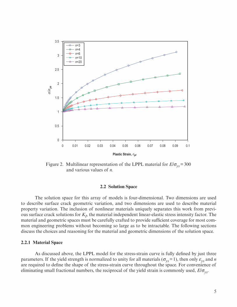
2. Multilinear representation of the LPPL material for E/sys = 300 and various values of n .............................................................................................. 5

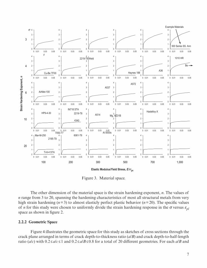
3. Material space ........................................................................................................... 7

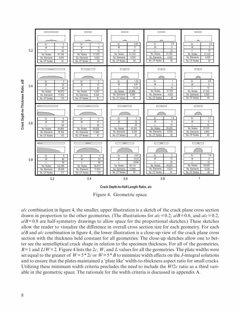
4. Geometric space ........................................................................................................ 8

5. Typical ¼ symmetric surface crack finite element mesh ............................................. 9

6. Cross section through the crack plane illustrating the characteristic lengths, rfa and rfb ..................................................................................................... 10

7. Method to choose far-field displacement values for FEMs based on a desired deformation level, M ................................................................................... 11

8. Cross section through the crack plane for two surface crack geometries with different physical dimensions but the same geometric proportions .................... 14

9. Comparison of the force versus CMOD response for models 1 and 2 ........................ 14

10. Comparison of Jtotal and Jel versus CMOD for models 1 and 2 ................................. 15

11. Comparison of Jtotal and Jel versus f for models 1 and 2 ........................................... 15

12. J(f) versus CMODn space .......................................................................................... 16

13. Conceptual illustration of the interpolation space ..................................................... 18

14. Illustration of (a) effect of truncating the solution space based on the average of the maximum CMODn values on the sn versus CMODn results, and (b) dividing the CMODn into even increments for sn versus CMODn interpolation .............................................................................................................. 20

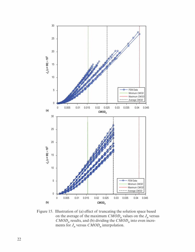
15. Illustration of (a) effect of truncating the solution space based on the average of the maximum CMODn values on the Jn versus CMODn results, and (b) dividing the CMODn into even increments for Jn versus CMODn interpolation .............................................................................................................. 22

vii

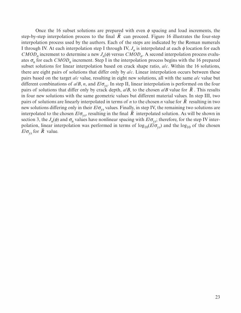
16. Conceptual illustration of the interpolation process. Arrow indicates interpolation direction ............................................................................................... 24

17. Comparison of results for (a) sn versus CMODn, (b) Jn(f = 90°) versus CMODn, and (c) Jn versus f for the final common loading condition for

the 16 solution subsets and the final interpolated result prior to interpolation step I to the desired a/c value ..................................................................................... 26

18. Comparison of results for (a) sn versus CMODn, (b) Jn(f = 90°) versus CMODn, and (c) Jn versus f for the final common loading condition for the eight solution subsets and the final interpolated result prior to interpolation step II to the desired a/B value ................................................................................... 27

19. Comparison of results for (a) sn versus CMODn, (b) Jn(f = 90°) versus CMODn, and (c) Jn versus f for the final common loading condition for the four solution subsets and the final interpolated result prior to interpolation step III to the desired n value ..................................................................................... 28

20. Comparison of results for (a) sn versus CMODn, (b) Jn(f = 90°) versus CMODn, and (c) Jn versus f for the final common loading condition for the two solution subsets and the final interpolated result prior to interpolation step IV to the desired E/sys value .............................................................................. 29

21. Comparison of results for (a) sn versus CMODn, (b) Jn(f = 90°) versus CMODn, and (c) Jn versus f for various a/B values, a/c = 0.6, n = 6, and E/sys = 300 .......................................................................................................... 31

22. Comparison of results for (a) sn versus CMODn, (b) Jn(f = 90°) versus CMODn, and (c) Jn versus f for a/B = 0.6, various a/c values, n = 6, and E/sys = 300 .......................................................................................................... 32

23. Comparison of results for (a) sn versus CMODn, (b) Jn(f = 90°) versus CMODn, and (c) Jn versus f for a/B = 0.6, a/c = 0.6, various n values, and E/sys = 300 .......................................................................................................... 33

24. Comparison of results for (a) sn versus CMODn, (b) Jn(f = 90°) versus CMODn, and (c) Jn versus f for a/B = 0.6, a/c = 0.6, n = 6, and various E/sys values ............................................................................................................... 34

25. Comparison of linear-elastic stress intensity correction factors from the NR equations to the values calculated from the 20 geometries in this study .............. 36

26. Normalized Jn(f = 90°) for each domain at the final load step for all 600 solutions .............................................................................................................. 37

LIST OF FIGURES (Continued)

viii

27. Percent difference in domains 9 and 10 Jn values for all f locations at the final load step for all 600 solutions ................................................................... 37

28. Comparison of benchmark model No. 1 FEM results and interpolated results for (a) P versus CMODn, (b) M versus CMODn, (c) benchmark FEM/interpolated results versus CMODn, (d) Jn versus CMODn at f = 30° and 90°, (e) Jn versus P at f = 30° and 90°, and (f) Jn versus f for CMODn values A and B ........................................................................................................... 40

29. Comparison of benchmark model No. 25 FEM results and interpolated results for (a) P versus CMODn, (b) M versus CMODn, (c) benchmark FEM/interpolated results versus CMODn, (d) Jn versus CMODn at f = 30° and 90°, (e) Jn versus P at f = 30° and 90°, and (f) Jn versus f for CMODn values A and B ........................................................................................................... 41

30. Round robin specimen configured for testing ............................................................. 43

31. Round robin specimen fracture surface with tearing location indicated ..................... 44

32. Round robin uniaxial tensile stress versus strain data compared with FEA and LPPL material fits ............................................................................................... 45

33. Influence of LPPL material choice on results for (a) P versus CMOD, (b) J(f = 17°) versus CMOD, and (c) J versus f .......................................................... 47

34. Interpolation, FEM, and RR participant results compared to experimental force versus CMOD response .................................................................................... 49

35. Comparison of interpolation, FEM, and RR participant results for J(f = 17°) versus CMOD ............................................................................................................ 50

36. Additional comparison of interpolation, FEM, and RR participant results for J(f = 17°) versus CMOD ...................................................................................... 51

37. Comparison of the sn versus CMODn results for geometries with differing 2c/W ..... 54

38. Comparison of the P versus CMODn results for geometries with differing 2c/W ....... 54

39. Comparison of the Jn(f = 90°) versus CMODn results for geometries with differing 2c/W .................................................................................................... 55

40. Comparison of the Jn versus f results for geometries with differing 2c/W at the maximum CMOD value of the 2c/W = 20 FEM ............................................... 55


ix


B1–B25 Comparison of benchmark model Nos. 1–25 FEM results and interpolated results for (a) P versus CMODn, (b) M versus CMODn, (c) benchmark FEM/interpolated results versus CMODn, (d) Jn versus CMODn at f = 30° and 90°, (e) Jn versus P at f = 30° and 90°, and (f) Jn versus f for CMODn values A and B .................................................................................................... 57

x

LIST OF TABLES

1. Benchmark FEM geometry and material values .......................................................... 38

2. Benchmark model numbers, model descriptions, and interpolated result comparisons ....................................................................................................... 39

3. Round robin FEM and interpolation method sensitivity study result comparisons ....................................................................................................... 45

4. Example database format for FEM solutions .............................................................. 82

xi

LIST OF ACRONYMS, ABBREVIATIONS, AND DESIGNATORS

2D two-dimensional

3D three-dimensional

C(T) compact tension

EPFM elastic-plastic fracture mechanics

EPRI Electric Power Research Institute

FEA finite element analysis

FEM finite element model

Int. interpolation solution (see table 3)

LEFM linear-elastic fracture mechanics

LPPL linear plus power law

NR Newman-Raju

RR round robin

RSM reference stress method

xii

NOMENCLATURE

2c total surface crack length

a crack depth

B plate thickness

c half surface crack length

CMOD crack mouth opening displacement

E elastic modulus

g geometry matrix

h1 nondimensional influence factor

Jel linear-elastic portion of Jtotal

Jn normalized J-integral value

Jf J-integral value at a given parametric crack front angle

KI mode I linear-elastic stress intensity factor

L plate length

M crack front deformation level

m material matrix

n strain hardening exponent

P force

R final interpolated result

rfa and rfb specimen characteristic lengths

W plate width

xiii

NOMENCLATURE (Continued)

α fitting constant

β fitting constant

γ fitting constant

δ axial displacement

δfar far-field axial displacement

ε engineering strain

εpl plastic strain

εys yield strain

λ geometry correction factor

ν Poisson’s ratio

s stress

sn normalized far-field stress

snet net section stress

sys material yield stress

f parametric crack front angle

1

TECHNICAL PUBLICATION

ELASTIC-PLASTIC J-INTEGRAL SOLUTIONS FOR SURFACE CRACKS IN TENSION USING AN INTERPOLATION METHODOLOGY

1. INTRODUCTION

Surface cracks are among the most common defects found in structural components and frequently reach failure once the limits of linear-elastic fracture mechanics (LEFM) have been exceeded and elastic-plastic fracture mechanics (EPFM) governs. For example, in the aerospace industry EPFM conditions commonly exist due to small critical crack sizes, thin walls, and high loading conditions inherent to lightweight, high-performance structures. Conversely, in the nuclear and petroleum industries EPFM conditions often prevail due to the use of lower strength, very high-toughness materials. EPFM assessment has become significantly more accessible through improved finite element interfaces such as FEACrack™ or ABAQUS® CAE,1,2 but unfortunately the cost of such assessments in analysis time remains a significant impediment to common use. Similar difficul-ties arise in assessing laboratory fracture toughness tests with surface cracks. In these tests, due to practical specimen size limitations, the material fracture toughness is commonly not reached until well beyond the LEFM limit. Surface crack fracture testing is hindered significantly by the lack of a readily available set of surface crack solutions for the nonspecialist to evaluate the elastic-plastic J-integral, crack mouth opening displacement (CMOD) values, or deformation state of a test speci-men at fracture. A convenient set of elastic-plastic surface crack solutions could help mitigate many of these obstacles.

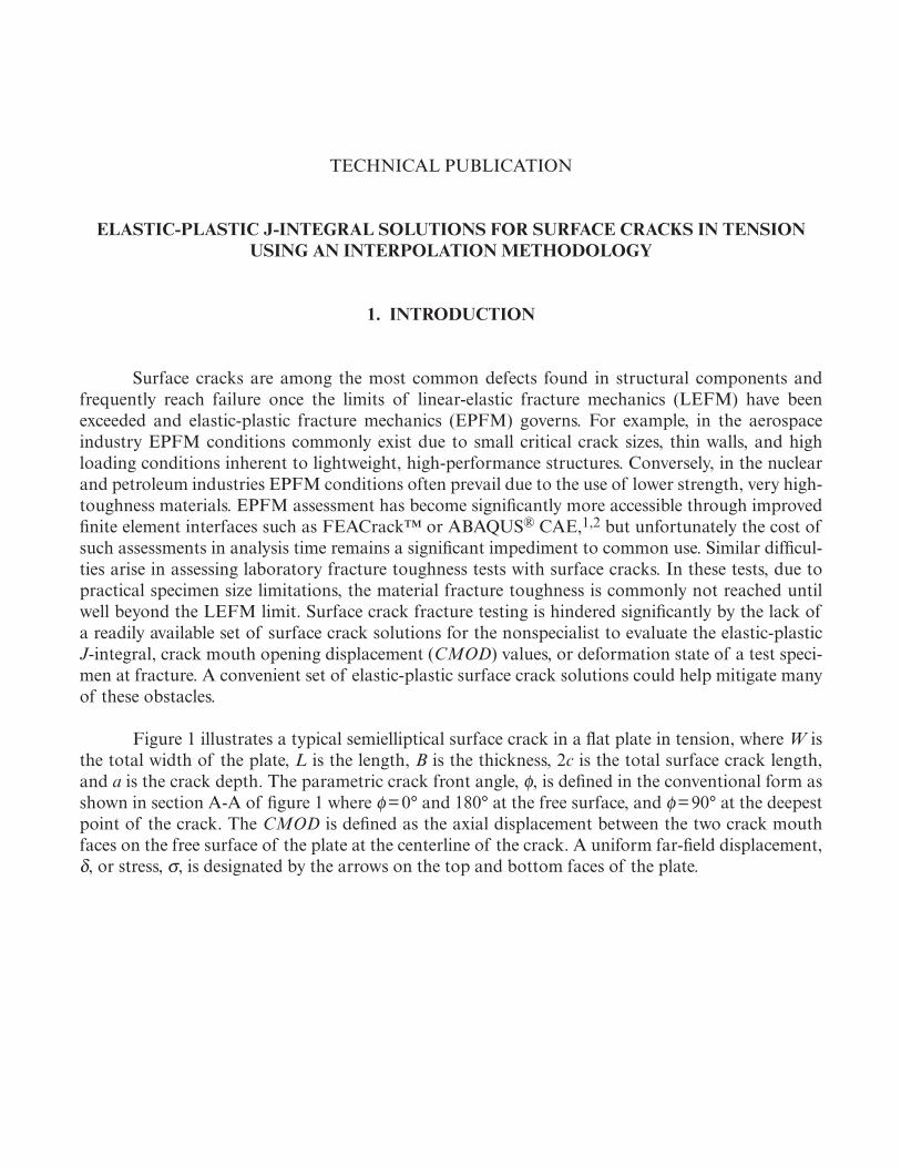
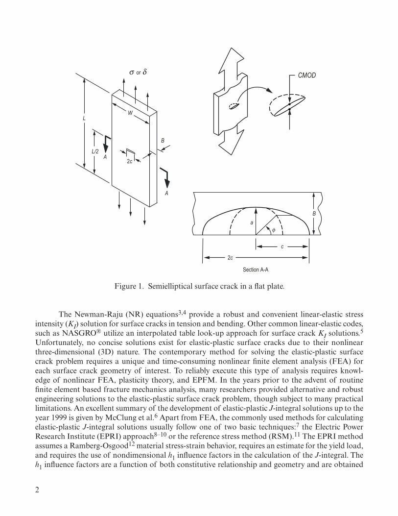
Figure 1 illustrates a typical semielliptical surface crack in a flat plate in tension, where W is the total width of the plate, L is the length, B is the thickness, 2c is the total surface crack length, and a is the crack depth. The parametric crack front angle, f, is defined in the conventional form as shown in section A-A of figure 1 where f= 0° and 180° at the free surface, and f= 90° at the deepest point of the crack. The CMOD is defined as the axial displacement between the two crack mouth faces on the free surface of the plate at the centerline of the crack. A uniform far-field displacement, δ, or stress, s, is designated by the arrows on the top and bottom faces of the plate.

2

W

2c

A

AL/2

L

B

φ

B

c

Section A-A

2co2c

a

σ δor CMOD

Figure 1. Semielliptical surface crack in a flat plate.

The Newman-Raju (NR) equations3,4 provide a robust and convenient linear-elastic stress intensity (KI) solution for surface cracks in tension and bending. Other common linear-elastic codes, such as NASGRO® utilize an interpolated table look-up approach for surface crack KI solutions.5 Unfortunately, no concise solutions exist for elastic-plastic surface cracks due to their nonlinear three-dimensional (3D) nature. The contemporary method for solving the elastic-plastic surface crack problem requires a unique and time-consuming nonlinear finite element analysis (FEA) for each surface crack geometry of interest. To reliably execute this type of analysis requires knowl-edge of nonlinear FEA, plasticity theory, and EPFM. In the years prior to the advent of routine finite element based fracture mechanics analysis, many researchers provided alternative and robust engineering solutions to the elastic-plastic surface crack problem, though subject to many practical limitations. An excellent summary of the development of elastic-plastic J-integral solutions up to the year 1999 is given by McClung et al.6 Apart from FEA, the commonly used methods for calculating elastic-plastic J-integral solutions usually follow one of two basic techniques:7 the Electric Power Research Institute (EPRI) approach8–10 or the reference stress method (RSM).11 The EPRI method assumes a Ramberg-Osgood12 material stress-strain behavior, requires an estimate for the yield load, and requires the use of nondimensional h1 influence factors in the calculation of the J-integral. The h1 influence factors are a function of both constitutive relationship and geometry and are obtained

3

from a fully plastic elastic-plastic finite element solution. Tables of h1 factors for surface cracks in flat plates have been generated by several researchers6,13–15 for limited combinations of material prop-erties, geometry values, and surface crack front angle, f. Yagawa et al.13 also developed influence factors for the fully plastic crack opening displacement for the geometries and materials covered in their study. In addition, Kim et al.16 performed investigations into the RSM for a limited number of surface crack geometries and Ramberg-Osgood material combinations.

The EPRI and RSM techniques have found wide application in analysis of structures but have limited application in the assessment of surface crack laboratory tests. To understand with sufficient precision the crack front conditions at the point the fracture toughness is reached in an experimental surface crack test requires knowledge of the force, P, versus CMOD response, the elastic-plastic deformation state of the specimen, and detailed knowledge of the J-integral versus f relationship as a function of deformation. The current RSM and EPRI solutions for surface cracks do not provide the user with the full P versus CMOD trace which serves as the most fundamental connection between experiment and analysis. The CMOD value provides the most robust predictor of the J-integral values at the crack tip.7,17 Most conventional fracture toughness test specimens such as the compact tension, C(T), or single edge notched bend are considered two-dimensional (2D) in nature and report a single value of fracture toughness representing the average driving force along the entire crack front. Conversely, the surface crack toughness test is highly 3D, and the toughness values are usually reported as a single, local value of toughness at a given f location along the crack front. Most of the current RSM and EPRI solutions only have solution values at a limited number of f locations. In addition, the EPRI and RSM techniques have J versus f relationships that are based on either linear-elastic solutions (RSM) or fully plastic solutions (EPRI) which do not capture the changes in the J versus f distribution and maximum J-integral location with increasing deformation.

To overcome these shortcomings and provide a simple and robust method for analyzing sur-face crack tension tests, the authors have developed and analyzed an array of 600, 3D nonlinear finite element models (FEMs) for surface cracks in flat plates under tension loading. The solution space covers a wide range of crack geometric parameters and material properties. The solution of this large array of nonlinear models was made practical by computer routines that automate the pro-cess of building the FEMs, running the nonlinear analyses, post-processing model results, and com-piling and organizing the solution results into multidimensional arrays. The authors have developed a methodology for interpolating between the geometric and material property variables that allows the user to estimate the J-integral solution around the surface crack perimeter (f) as a function of loading condition from the linear-elastic regime through the elastic-plastic regime. In addition to the J-integral solution, the complete force versus CMOD record is estimated. The user of this interpo-lated solution space need only know the crack and plate geometry and the basic material flow prop-erties to reliably evaluate the full surface crack J-integral and force versus CMOD solution; thus, a solution can be obtained very rapidly by users without EPFM modeling experience.

4

2. COMPUTATIONAL PROCEDURES

This project is logistically intense. Though computationally, each part of the process of build-ing this new solution space follows mostly well-established paths, combining those parts effectively into a functional whole requires planning at every level. This section provides insight into the basic computational procedures used in the FEMs which constitutes the solution space as well as the parameters of the geometric and material property variables that define the overall solution space. Briefly discussed in the conclusion are the logistics of building, executing, and then assembling the solution space—made practical only through automation.

2.1 Constitutive Model

The constitutive model for this study employs incremental von Mises plasticity theory in a conventional small geometry change (small strain) setting. The material is assumed to be isotronic and homogenous with flow behavior following a linear plus power law (LPPL) representation of the stress-strain response. For the LPPL model, the uniaxial stress-strain curve follows a linear then power law model given by

εεys

=σσ ys

ε ≤ εys ; εεys

=σσ ys

⎛

⎝⎜

⎞

⎠⎟

n

ε > εys , (1)

where εis engineering strain, n is the strain hardening exponent,s is engineering stress, sys is a rep-resentative yield stress, and εys is a corresponding yield strain defined by εys = sys /E, with the elastic modulus, E. For this analytical work, sys is equivalent to the proportional limit and defines the lim-its of the initial linear-elastic portion of the response. This approach to modeling the stress-strain response has numerous advantages in this study: first, the model lends itself to easy implementation in the planned material space because the curve is fully defined by three parameters (sys, εys or E, and n); second, the model faithfully represents the stress-strain response of a large majority of structural metals; and third, unlike the commonly used Ramberg-Osgood model, prior to exceeding the yield strain, the LPPL model is purely linear-elastic, and thus does not prematurely accumulate plastic strain. Unlike the research FEA code utilized for this study, WARP3D,18 most commercial finite ele-ment codes do not natively support the LPPL model for plasticity analysis. Therefore, to make the analysis methods used in this study more universally repeatable in other analysis codes, the smooth LPPL representation of the material response forε> εys was discretized into 20 line segments for use in the commonly available, multilinear stress-strain curve representation. In this way, the common and convenient way of describing the plastic hardening behavior through the hardening exponent, n, could be retained but the analysis performed in a way that is not dependent on the availability of a native LPPL model. The plastic strain, εpl, increments for each multilinear line segment were gra-dated from initially fine increments of 0.001 for eight line segments, to 0.005 for four line segments and then to 0.01 for the remaining seven line segments to ensure a smooth transition from linear-elastic to nonlinear behavior and to smoothly capture the power law hardening behavior. Figure 2 illustrates the multilinear representation of the LPPL plastic response for a material with a yield strain,

εys = 0.003 (normalized elastic modulus of E/sys=300) and various n values.

5

Plastic Strain,

0 0.01 0.02 0.03 0.04 0.05 0.06 0.07 0.08 0.09 0.10

0.5

1

1.5

2

2.5

3

3.5

pl

n=3n=4n=6n=10n=20

ε

σσ /

ys

Figure 2. Multilinear representation of the LPPL material for E/sys = 300 and various values of n.

2.2 Solution Space

The solution space for this array of models is four-dimensional. Two dimensions are used to describe surface crack geometric variation, and two dimensions are used to describe material property variation. The inclusion of nonlinear materials uniquely separates this work from previ-ous surface crack solutions for KI, the material independent linear-elastic stress intensity factor. The material and geometric spaces must be carefully crafted to provide sufficient coverage for most com-mon engineering problems without becoming so large as to be intractable. The following sections discuss the choices and reasoning for the material and geometric dimensions of the solution space.

2.2.1 Material Space

As discussed above, the LPPL model for the stress-strain curve is fully defined by just three parameters. If the yield strength is normalized to unity for all materials (sys = 1), then only εys and n are required to define the shape of the stress-strain curve throughout the space. For convenience of eliminating small fractional numbers, the reciprocal of the yield strain is commonly used, E/sys.

6

Figure 3 illustrates the material space for the study described in terms of the six E/sys and five n values resulting in 30 different material combinations. In all cases, sys = 1 and Poisson’s ratio, ν= 0.3. The names of several common engineering materials are overlaid on the material matrix in figure 3 to illustrate how some common materials are represented in the material matrix. The low E/sys values of 100 to 200 are materials capable of high values of elastic strain, thus they have low elastic modulus and relatively high yield strength, such as many high-performance titanium and alu-minum alloys. The opposite end of the E/sys space with values of E/sys=1,000 have very little elastic strain capability due to high elastic modulus and low yield strength. Austenitic stainless steels are a common example of this material class. To practitioners not accustomed to considering materials based on the E/sys ratio, it is important to realize that, for a fixed hardening exponent, n, the nonlin-ear material response is governed by this ratio. Materials that may not seem alike from an engineering perspective are actually equivalent in their nonlinear response. For example, consider three materials with similar n and equivalent yield strains such that E/sys = 400 in each case. This could easily be an aluminum alloy with yield strength around 180 MPa, a titanium alloy with yield strength around 275 MPa, or a steel alloy with yield strength around 500 MPa. The normalized nonlinear response is the same in each case. This will be discussed further in a following section on normalization schemes. The effect of E/sys on the load, P, versus CMOD behavior (and the resulting J-integral values) is strongest for lower values of E/sys; therefore, the authors chose smaller increments of E/sys for E/sys ≤ 300 to provide more uniform coverage over the solution space.

7

0 0.01 0.03 0.050

1

2

3

4

0 0.01 0.03 0.050

1

2

3

4

0 0.01 0.03 0.050

1

2

3

4

0 0.01 0.03 0.050

1

2

3

4

0 0.01 0.03 0.050

1

2

3

4

0 0.01 0.03 0.050

1

2

3

4

0 0.01 0.03 0.050

1

2

3

4

0 0.01 0.03 0.050

1

2

3

4

0 0.01 0.03 0.050

1

2

3

4

0 0.01 0.03 0.050

1

2

3

4

0 0.01 0.03 0.050

1

2

3

4

0 0.01 0.03 0.050

1

2

3

4

0 0.01 0.03 0.050

1

2

3

4

0 0.01 0.03 0.050

1

2

3

4

0 0.01 0.03 0.050

1

2

3

4

0 0.01 0.03 0.050

1

2

3

4

0 0.01 0.03 0.050

1

2

3

4

0 0.01 0.03 0.050

1

2

3

4

0 0.01 0.03 0.050

1

2

3

4

0 0.01 0.03 0.050

1

2

3

4

0 0.01 0.03 0.050

1

2

3

4

0 0.01 0.03 0.050

1

2

3

4

0 0.01 0.03 0.050

1

2

3

4

0 0.01 0.03 0.050

1

2

3

4

0 0.01 0.03 0.050

1

2

3

4

0 0.01 0.03 0.050

1

2

3

4

0 0.01 0.03 0.050

1

2

3

4

0 0.01 0.03 0.050

1

2

3

4

0 0.01 0.03 0.050

1

2

3

4

0 0.01 0.03 0.050

1

2

3

4

20

10

6

4

3

100 200 300 500 700 1,000

2219-T8

2195-T8

300 Series SS. Ann

Example Materials

2219-T8 Weld

Ti-6-4 STA

7050-T7 Mar-M-250

AirMet-100

A514

A537 A572

A36

1010 HR

6061-T6 Al 5000s

Hastelloy-X IN718 STA

Haynes 188

Be

Cu-Be TF00

4340

Mg, AZ31B HP9-4-30

Elastic Modulus/Yield Stress, E / ys

Stra

in H

arde

ning

Exp

onen

t, n

σ

σ

ε

Figure 3. Material space.

The other dimension of the material space is the strain hardening exponent, n. The values of n range from 3 to 20, spanning the hardening characteristics of most all structural metals from very high strain hardening (n = 3) to almost elasticly perfect plastic behavior (n = 20). The specific values of n for this study were chosen to uniformly divide the strain hardening response in the s versus εpl space as shown in figure 2.

2.2.2 Geometric Space

Figure 4 illustrates the geometric space for this study as sketches of cross sections through the crack plane arranged in terms of crack depth-to-thickness ratio (a/B) and crack depth-to-half-length ratio (a/c) with 0.2 ≤ a/c ≤ 1 and 0.2 ≤ a/B ≤ 0.8 for a total of 20 different geometries. For each a/B and

8

a/c combination in figure 4, the smaller, upper illustration is a sketch of the crack plane cross section drawn in proportion to the other geometries. (The illustrations for a/c = 0.2, a/B = 0.6, and a/c = 0.2, a/B = 0.8 are half-symmetry drawings to allow space for the proportional sketches.) These sketches allow the reader to visualize the difference in overall cross section size for each geometry. For each a/B and a/c combination in figure 4, the lower illustration is a close-up view of the crack plane cross section with the thickness held constant for all geometries. The close-up sketches allow one to bet-ter see the semielliptical crack shape in relation to the specimen thickness. For all of the geometries, B = 1 and L/W = 2. Figure 4 lists the 2c, W, and L values for all the geometries. The plate widths were set equal to the greater of W = 5 * 2c or W = 5 * B to minimize width effects on the J-integral solutions and to ensure that the plates maintained a ‘plate like’ width-to-thickness aspect ratio for small cracks. Utilizing these minimum width criteria precludes the need to include the W/2c ratio as a third vari-able in the geometric space. The rationale for the width criteria is discussed in appendix A.

Figure 4. Geometric space.

0.2 0.4 0.6 0.8 1

0.2

0.8

0.6

0.4

2c 2W 10L 20

No. Nodes 41,146No. Elements 8,876No. CF Nodes 91

2c 4W 20L 40


2c 6W 30L 60


2c 8W 40L 80


2c 4WL

No. NodesNo. ElementsNo. CF Nodes

2c 1W 5L 10


2c 2W 10L 20


2c 3W 15L 30


1.62040

80,87217,632

133

2c 0.67W 5L 10


2c 1.33W 6.67L 13.34


2c 2W 10L 20


2c 2.67W 13.33L 26.66


2c 0.5W 5L 10


2c 1W 5L 10


2c 1.5W 8L 15


2c 2W 10L 20


2c 0.4W 5L 10


2c 0.8W 5L 10


2c 1.2W 6L 12


2cW 8L 16


Crack Depth-to-Half-Length Ratio, a/c

Crac

k Dep

th-to

-Thi

ckne

ss R

atio

, a/B

9

2.3 Finite Element Models

A total of 600 nonlinear finite element analyses were required to perform the analysis of the 30 material and 20 geometric combinations. All of the finite element models were created using the commercial finite element mesh creation and post-processing tool, FEACrack,1 and the analyses were performed using the freely available research code, WARP3D version 16.3.1.18

2.3.1 Finite Element Model Details

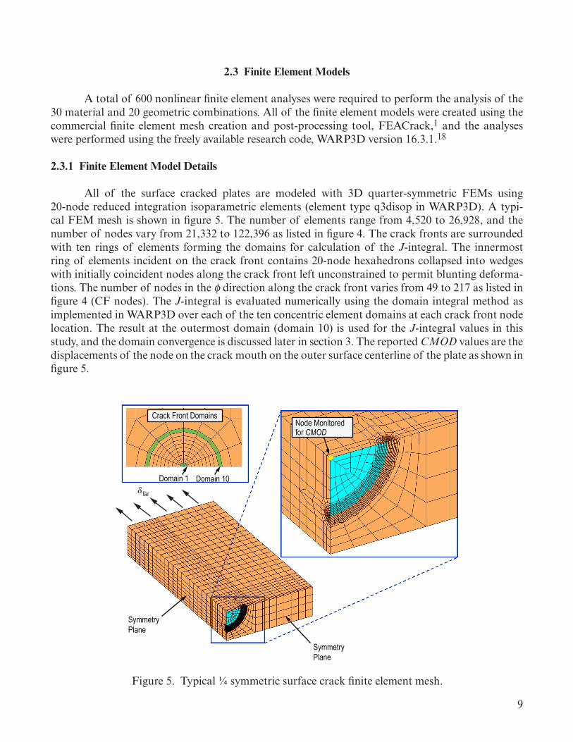
All of the surface cracked plates are modeled with 3D quarter-symmetric FEMs using 20-node reduced integration isoparametric elements (element type q3disop in WARP3D). A typi-cal FEM mesh is shown in figure 5. The number of elements range from 4,520 to 26,928, and the number of nodes vary from 21,332 to 122,396 as listed in figure 4. The crack fronts are surrounded with ten rings of elements forming the domains for calculation of the J-integral. The innermost ring of elements incident on the crack front contains 20-node hexahedrons collapsed into wedges with initially coincident nodes along the crack front left unconstrained to permit blunting deforma-tions. The number of nodes in the f direction along the crack front varies from 49 to 217 as listed in figure 4 (CF nodes). The J-integral is evaluated numerically using the domain integral method as implemented in WARP3D over each of the ten concentric element domains at each crack front node location. The result at the outermost domain (domain 10) is used for the J-integral values in this study, and the domain convergence is discussed later in section 3. The reported CMOD values are the displacements of the node on the crack mouth on the outer surface centerline of the plate as shown in figure 5.

SymmetryPlane

SymmetryPlane

Node Monitoredfor CMOD

Domain 1 Domain 10

Crack Front Domains

δ far

Figure 5. Typical ¼ symmetric surface crack finite element mesh.

10

2.3.2 Boundary Conditions and Loading

The FEMs are loaded with 20 to 30 uniform load steps with an average of 2 to 5 Newton iterations for convergence within each step to a tight tolerance on residual nodal forces. Symmetry planes are enforced through setting the normal nodal displacements on the plane equal to zero. Uni-form axial displacements, δfar , are applied to all of the nodes on the top surface of the plate to apply tension. The intent was to apply sufficient displacement to deform the models far into an elastic-plastic regime, but not so much that the models would fail to converge on the last analysis step. Since hundreds of nonlinear models were run, it was not practical to ‘hand pick’ a unique value for each displacement boundary condition—an automated method had to be employed.

The δfar boundary conditions for the FEMs are applied in a two-step process. First, the LPPL equation is used to calculate the net section stress, snet, corresponding to εpl = 0.1%. This stress is then used to calculate a linear approximation of the far-field displacement using the equation

! far ="netL

2E , (2)

where the factor of ½ is due to symmetry. All of the FEMs were successfully run with the δfar values from equation (2) applied, and the models were checked for the deformation level, M, where M is defined as

M =rφσ ys

Jφ . (3)

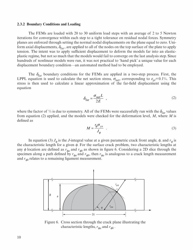
In equation (3) Jf is the J-integral value at a given parametric crack front angle, f, and rf

is the characteristic length for a givenf. For the surface crack problem, two characteristic lengths at any f location are defined as rfa and rfb as shown in figure 6. Considering a 2D slice through the specimen along a path defined by rfa and rfb, then rfa

is analogous to a crack length measurement and rfb relates to a remaining ligament measurement.

aB

2c

rφ b

rφ aφ

Figure 6. Cross section through the crack plane illustrating the characteristic lengths, rfa and rfb .

11

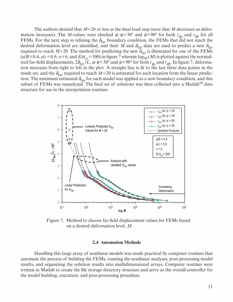
The authors desired that M ≈ 20 or less at the final load step (note that M decreases as defor-mation increases). The M-values were checked at f= 30° and f= 90° for both rfa

and rfb for all FEMs. For the next step in refining the δfar boundary condition, the FEMs that did not reach the desired deformation level are identified, and their M and δfar data are used to predict a new δfar required to reach M ≈ 20. The method for predicting the new δfar is illustrated for one of the FEMs (a/B = 0.4, a/c = 0.6, n = 6, and E/sys = 500) in figure 7 wherein log10 (M) is plotted against the normal-ized far-field displacements, 2δfar /L, atf= 30° and f= 90° for both rfa

and rfb. In figure 7, deforma-tion increases from right to left in the plot. A straight line is fit to the last three data points in the result set, and the δfar required to reach M =20 is estimated for each location from the linear predic-tion. The minimum estimated δfar for each model was applied as a new boundary condition, and this subset of FEMs was reanalyzed. The final set of solutions was then collected into a Matlab19 data structure for use in the interpolation routines.

101 102 103 104 105 1060

1

2

3

4

5

6

7

8

log M

! ! ! ! !Linearly Predicted δ far Values for M = 20

Analysis withUpdated δ far values

IncreasingDeformation

2δfa

r / L × 10

3

Linear Predictionfor δ far

rφ a for φ = 30rφ b for φ = 30rφ a for φ = 90rφ b for φ = 90Updated Analysis

a/B = 0.4a/c = 0.6n = 6E/ ys= 500σ

Figure 7. Method to choose far-field displacement values for FEMs based on a desired deformation level, M.

2.4 Automation Methods

Handling this large array of nonlinear models was made practical by computer routines that automate the process of building the FEMs, running the nonlinear analyses, post-processing model results, and organizing the solution results into multidimensional arrays. Computer routines were written in Matlab to create the file storage directory structure and serve as the overall controller for the model building, execution, and post-processing procedure.

12

The FEMs were built using FEACrack in batch control mode on a 64-bit Windows XP com-puter. FEACrack uses a text-based input file to control all the model parameters for a given FEM. The authors developed Matlab scripts that read in a ‘baseline’ FEACrack input file for a surface crack plate and modified the file to include the desired plate dimensions, crack dimensions, mate-rial properties, and boundary conditions. The script then executes FEACrack in batch mode to build the appropriate input file for WARP3D and saves the file with an appropriate filename in the desired directory. This process was automated to prepare the required 600 input files for analysis. The WARP3D input files were then moved to a 64-bit Linux server for efficient parallel processing analy-sis. Once the FEAs were complete, the WARP3D binary packet result files were transferred to the 64-bit Windows XP computer and were post-processed in batch mode with FEACrack using another set of Matlab generated scripts. These post-processing steps resulted in a set of 600 text-based result files from FEACrack that contained all of the pertinent model result data. A set of Matlab scripts were then used to consolidate the full data set into arrays of J-integral versus f values, far-field stresses, and CMOD values in an easily indexed Matlab data structure.

2.5 Interpolation Methodology

The interpolation methods developed and implemented in this study involve a normalization scheme used to scale the solutions. This scheme is described below along with a brief exemplar case study. The interpolation process takes place in this dimensionless, normalized space. The interpola-tion methods are described on a step-by-step basis.

2.5.1 Normalization Scheme

To derive useful results from the solution space, interpolation within the geometry and mate-rial dimensions is necessary, but scaling of the solutions with respect to geometry and material is also required. To simplify scaling of the solution space, it is advantageous, but not required, to have the solution space normalized to a dimensionless state. In this fashion, once interpolation is complete within the space, the resulting dimensionless interpolated solution can be easily scaled by to a dimen-sioned state by multiplying by representative length and stress scaling factors for the actual geometry. There are three primary results in the solution set that need to be normalized: J, CMOD, and far-field stress, s. By dimensional analysis, it is clear that the J-integral is conveniently normalized by a product of stress and length, therefore the normalized J-integral value, Jn, can be written as

Jn =J

σ ysB . (4)

In this case, the normalizing stress is chosen to be the material yield strength (proportional limit) represented in the LPPL stress-strain curve model, and the normalizing length is chosen to be the plate thickness, B. These are particularly convenient normalizing factors because, as discussed previously, both sys and B were defined to have unit value in the model space. Thus, the J-integral value from the analysis does not change when normalized. The same follows for the CMOD and far-field stress results where

CMODn =

CMODB

, (5)

13

and the normalized far-field stress, sn, is

σn =σσ ys

. (6)

Starting from this normalized space, a dimensional result is easily obtained by reversing the normalization by multiplying by the appropriate dimensional factors, BD and sysD, the thickness and yield strength, respectively, of the actual specimen or structure. Letting JD, CMODD, and sD represent the dimensional results;

JD = Jn *σ ysD * BD , (7)

CMODD =CMODn * BD , (8)

and

σD = σn *σ ysD . (9)

The dimensional force, PD, associated with the far stress, sD, can be obtained by simple mechanics following similar form:

PD = σn *WD * BD , (10)

where WD is the dimensional width of the plate.

2.5.2 Normalization Case Study

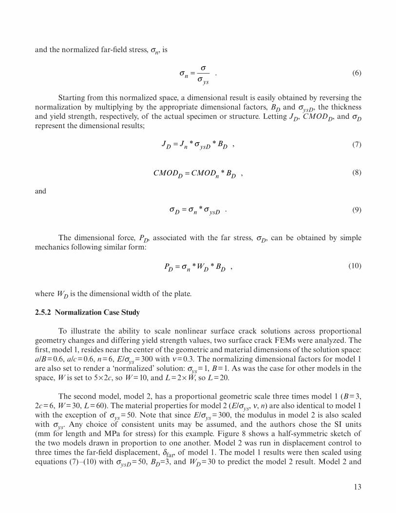
To illustrate the ability to scale nonlinear surface crack solutions across proportional geometry changes and differing yield strength values, two surface crack FEMs were analyzed. The first, model 1, resides near the center of the geometric and material dimensions of the solution space: a/B = 0.6, a/c = 0.6, n = 6, E/sys = 300 with ν = 0.3. The normalizing dimensional factors for model 1 are also set to render a ‘normalized’ solution: sys = 1, B = 1. As was the case for other models in the space, W is set to 5 ×2c, so W = 10, and L = 2 ×W, so L = 20.

The second model, model 2, has a proportional geometric scale three times model 1 (B = 3, 2c = 6, W = 30, L = 60). The material properties for model 2 (E/sys, ν, n) are also identical to model 1 with the exception of sys = 50. Note that since E/sys = 300, the modulus in model 2 is also scaled with sys. Any choice of consistent units may be assumed, and the authors chose the SI units (mm for length and MPa for stress) for this example. Figure 8 shows a half-symmetric sketch of the two models drawn in proportion to one another. Model 2 was run in displacement control to three times the far-field displacement, δfar, of model 1. The model 1 results were then scaled using equations (7) –(10) with sysD = 50, BD=3, and WD = 30 to predict the model 2 result. Model 2 and

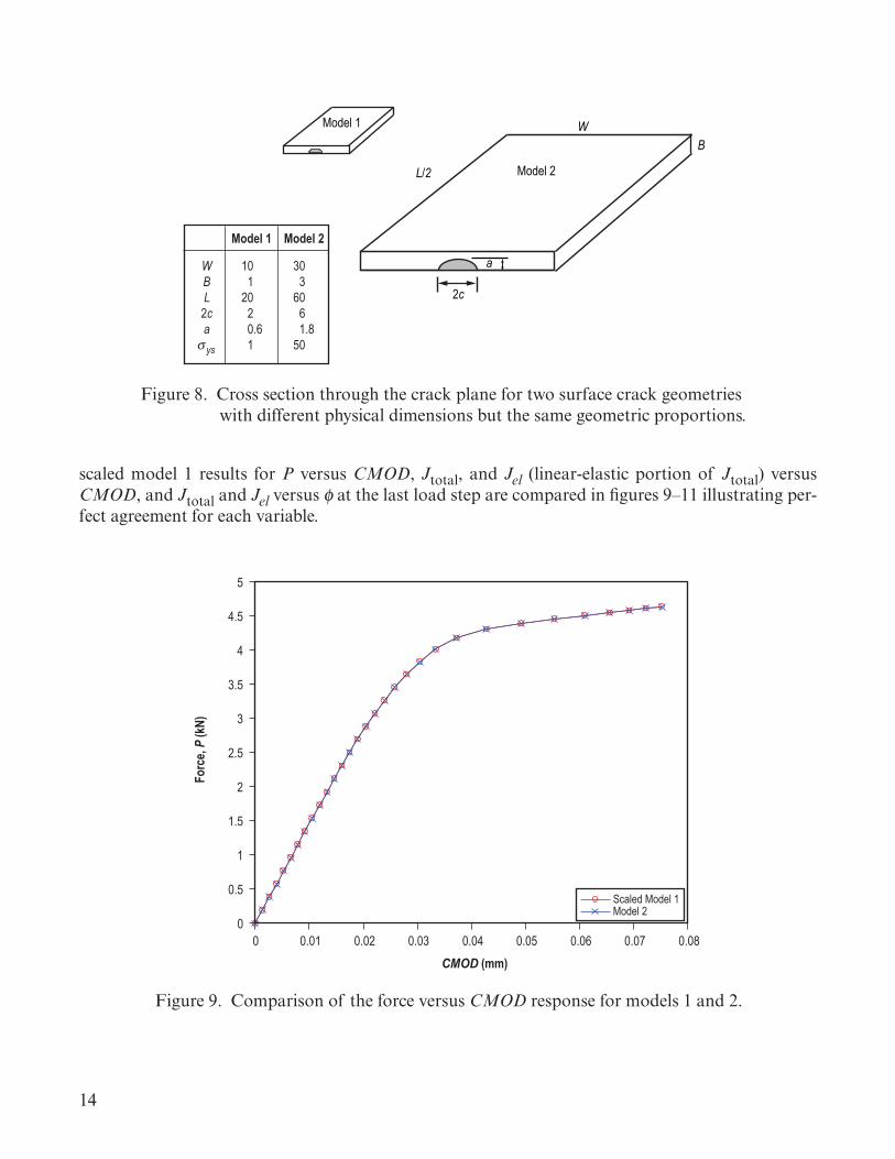
14

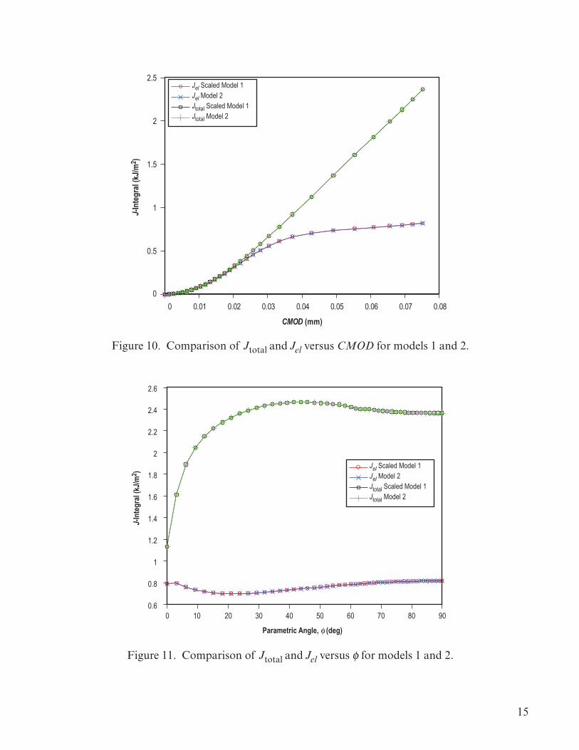
scaled model 1 results for P versus CMOD, Jtotal, and Jel (linear-elastic portion of Jtotal) versus CMOD, and Jtotal and Jel versus f at the last load step are compared in figures 9–11 illustrating per-fect agreement for each variable.

0 0.01 0.02 0.03 0.04 0.05 0.06 0.07 0.080

0.5

1

1.5

2

2.5

3

3.5

4

4.5

5

CMOD (mm)

Forc

e, P

(kN)

Scaled Model 1Model 2

Figure 9. Comparison of the force versus CMOD response for models 1 and 2.

Figure 8. Cross section through the crack plane for two surface crack geometries with different physical dimensions but the same geometric proportions.

Model 2

Model 1 W B

L/2

2c

a

Model 1 Model 2

WBL2ca

ysσ

10 1

20 2 0.61

30 3

60 6 1.8

50

15

0 0.01 0.02 0.03 0.04 0.05 0.06 0.07 0.080

0.5

1

1.5

2

2.5

CMOD (mm)

J-In

tegr

al (k

J/m2 )

Jel Scaled Model 1Jel Model 2Jtotal Scaled Model 1Jtotal Model 2

Figure 10. Comparison of Jtotal and Jel versus CMOD for models 1 and 2.

0 10 20 30 40 50 60 70 80 900.6

0.8

1

1.2

1.4

1.6

1.8

2

2.2

2.4

2.6

Jel Scaled Model 1Jel Model 2Jtotal Scaled Model 1Jtotal Model 2

Parametric Angle, φ (deg)

J-In

tegr

al (k

J/m2 )

Figure 11. Comparison of Jtotal and Jel versus f for models 1 and 2.

16

2.6 Solution Space Interpolation

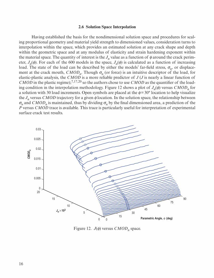
Having established the basis for the nondimensional solution space and procedures for scal-ing proportional geometry and material yield strength to dimensioned values, consideration turns to interpolation within the space, which provides an estimated solution at any crack shape and depth within the geometric space and at any modulus of elasticity and strain hardening exponent within the material space. The quantity of interest is the Jn value as a function of f around the crack perim-eter, Jn(f). For each of the 600 models in the space, Jn(f) is calculated as a function of increasing load. The state of the load can be described by either the models’ far-field stress, sn, or displace-ment at the crack mouth, CMODn. Though sn (or force) is an intuitive descriptor of the load, for elastic-plastic analysis, the CMOD is a more reliable predictor of J (J is nearly a linear function of CMOD in the plastic regime);7,17,20 so the authors chose to use CMOD as the quantifier of the load-ing condition in the interpolation methodology. Figure 12 shows a plot of Jn(f) versus CMODn for a solution with 30 load increments. Open symbols are placed at the f = 30° location to help visualize the Jn versus CMOD trajectory for a given f location. In the solution space, the relationship between sn and CMODn is maintained, thus by dividing sn by the final dimensioned area, a prediction of the P versus CMOD trace is available. This trace is particularly useful for interpretation of experimental surface crack test results.

015

3045

6075

90

0

5

10

15

200

0.005

0.01

0.015

0.02

0.025

0.03

CMOD

n


Jn × 103

Figure 12. J(f) versus CMODn space.

17

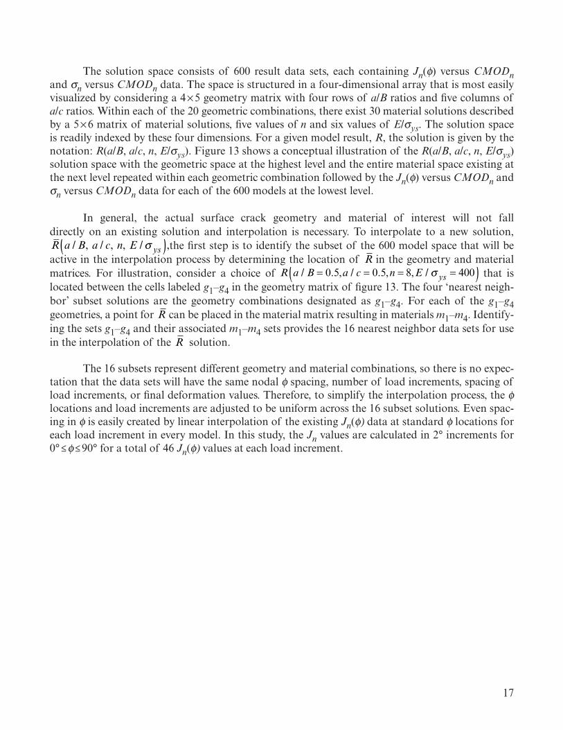
The solution space consists of 600 result data sets, each containing Jn(f) versus CMODn and sn versus CMODn data. The space is structured in a four-dimensional array that is most easily visualized by considering a 4 ×5 geometry matrix with four rows of a/B ratios and five columns of a/c ratios. Within each of the 20 geometric combinations, there exist 30 material solutions described by a 5 ×6 matrix of material solutions, five values of n and six values of E/sys. The solution space is readily indexed by these four dimensions. For a given model result, R, the solution is given by the notation: R(a/B, a/c, n, E/sys). Figure 13 shows a conceptual illustration of the R(a/B, a/c, n, E/sys) solution space with the geometric space at the highest level and the entire material space existing at the next level repeated within each geometric combination followed by the Jn(f) versus CMODn and sn versus CMODn data for each of the 600 models at the lowest level.

In general, the actual surface crack geometry and material of interest will not fall directly on an existing solution and interpolation is necessary. To interpolate to a new solution, R a / B, a / c, n, E /! ys( ),the first step is to identify the subset of the 600 model space that will be active in the interpolation process by determining the location of R in the geometry and material matrices. For illustration, consider a choice of

R a / B = 0.5,a / c = 0.5,n = 8,E / σ ys = 400( ) that is

located between the cells labeled g1–g4 in the geometry matrix of figure 13. The four ‘nearest neigh-bor’ subset solutions are the geometry combinations designated as g1–g4. For each of the g1–g4 geometries, a point for R can be placed in the material matrix resulting in materials m1–m4. Identify-ing the sets g1–g4 and their associated m1–m4 sets provides the 16 nearest neighbor data sets for use in the interpolation of the R solution.

The 16 subsets represent different geometry and material combinations, so there is no expec-tation that the data sets will have the same nodal f spacing, number of load increments, spacing of load increments, or final deformation values. Therefore, to simplify the interpolation process, the flocations and load increments are adjusted to be uniform across the 16 subset solutions. Even spac-ing in f is easily created by linear interpolation of the existing Jn(f) data at standard f locations for each load increment in every model. In this study, the Jn values are calculated in 2° increments for 0° ≤ f ≤ 90° for a total of 46 Jn(f) values at each load increment.

18

0 0.01 0.03 0.050

1

2

3

4

0 0.01 0.03 0.050

1

2

3

4

0 0.01 0.03 0.050

1

2

3

4

0 0.01 0.03 0.050

1

2

3

4

0 0.01 0.03 0.050

1

2

3

4

0 0.01 0.03 0.050

1

2

3

4

0 0.01 0.03 0.050

1

2

3

4

0 0.01 0.03 0.050

1

2

3

4

0 0.01 0.03 0.050

1

2

3

4

0 0.01 0.03 0.050

1

2

3

4

0 0.01 0.03 0.050

1

2

3

4

0 0.01 0.03 0.050

1

2

3

4

0 0.01 0.03 0.050

1

2

3

4

0 0.01 0.03 0.050

1

2

3

4

0 0.01 0.03 0.050

1

2

3

4

0 0.01 0.03 0.050

1

2

3

4

0 0.01 0.03 0.050

1

2

3

4

0 0.01 0.03 0.050

1

2

3

4

0 0.01 0.03 0.050

1

2

3

4

0 0.01 0.03 0.050

1

2

3

4

0 0.01 0.03 0.050

1

2

3

4

0 0.01 0.03 0.050

1

2

3

4

0 0.01 0.03 0.050

1

2

3

4

0 0.01 0.03 0.050

1

2

3

4

0 0.01 0.03 0.050

1

2

3

4

0 0.01 0.03 0.050

1

2

3

4

0 0.01 0.03 0.050

1

2

3

4

0 0.01 0.03 0.050

1

2

3

4

0 0.01 0.03 0.050

1

2

3

4

0 0.01 0.03 0.050

1

2

3

4

20

10

6

4

3

n

0 15 30 45 60 75 90

05

1015

200

0.005

0.01

0.015

0.02

0.025

0.03

0.2 0.4 0.6 0.8 1

0.2

0.8

0.6

0.4

0 0.01 0.03 0.050

1

2

3

4

0 0.01 0.03 0.050

1

2

3

4

0 0.01 0.03 0.050

1

2

3

4

0 0.01 0.03 0.050

1

2

3

4

0 0.01 0.03 0.050

1

2

3

4

0 0.01 0.03 0.050

1

2

3

4

0 0.01 0.03 0.050

1

2

3

4

0 0.01 0.03 0.050

1

2

3

4

0 0.01 0.03 0.050

1

2

3

4

0 0.01 0.03 0.050

1

2

3

4

0 0.01 0.03 0.050

1

2

3

4

0 0.01 0.03 0.050

1

2

3

4

0 0.01 0.03 0.050

1

2

3

4

0 0.01 0.03 0.050

1

2

3

4

0 0.01 0.03 0.050

1

2

3

4

0 0.01 0.03 0.050

1

2

3

4

0 0.01 0.03 0.050

1

2

3

4

0 0.01 0.03 0.050

1

2

3

4

0 0.01 0.03 0.050

1

2

3

4

0 0.01 0.03 0.050

1

2

3

4

0 0.01 0.03 0.050

1

2

3

4

0 0.01 0.03 0.050

1

2

3

4

0 0.01 0.03 0.050

1

2

3

4

0 0.01 0.03 0.050

1

2

3

4

0 0.01 0.03 0.050

1

2

3

4

0 0.01 0.03 0.050

1

2

3

4

0 0.01 0.03 0.050

1

2

3

4

0 0.01 0.03 0.050

1

2

3

4

0 0.01 0.03 0.050

1

2

3

4

0 0.01 0.03 0.050

1

2

3

4

20

10

6

4

3

n

g1

g1 g2

g3 g4

g2

g3 g4

m1

m1 m2

m3 m4

0 0.005 0.01 0.015 0.02 0.025 0.030

0.2

0.4

0.6

0.8

1

1.2

0 0.01 0.03 0.050

1

2

3

4

0 0.01 0.03 0.050

1

2

3

4

0 0.01 0.03 0.050

1

2

3

4

0 0.01 0.03 0.050

1

2

3

4

0 0.01 0.03 0.050

1

2

3

4

0 0.01 0.03 0.050

1

2

3

4

0 0.01 0.03 0.050

1

2

3

4

0 0.01 0.03 0.050

1

2

3

4

0 0.01 0.03 0.050

1

2

3

4

0 0.01 0.03 0.050

1

2

3

4

0 0.01 0.03 0.050

1

2

3

4

0 0.01 0.03 0.050

1

2

3

4

0 0.01 0.03 0.050

1

2

3

4

0 0.01 0.03 0.050

1

2

3

4

0 0.01 0.03 0.050

1

2

3

4

0 0.01 0.03 0.050

1

2

3

4

0 0.01 0.03 0.050

1

2

3

4

0 0.01 0.03 0.050

1

2

3

4

0 0.01 0.03 0.050

1

2

3

4

0 0.01 0.03 0.050

1

2

3

4

0 0.01 0.03 0.050

1

2

3

4

0 0.01 0.03 0.050

1

2

3

4

0 0.01 0.03 0.050

1

2

3

4

0 0.01 0.03 0.050

1

2

3

4

0 0.01 0.03 0.050

1

2

3

4

0 0.01 0.03 0.050

1

2

3

4

0 0.01 0.03 0.050

1

2

3

4

0 0.01 0.03 0.050

1

2

3

4

0 0.01 0.03 0.050

1

2

3

4

0 0.01 0.03 0.050

1

2

3

4

20

10

6

4

3

n

0 0.01 0.03 0.050

1

2

3

4

0 0.01 0.03 0.050

1

2

3

4

0 0.01 0.03 0.050

1

2

3

4

0 0.01 0.03 0.050

1

2

3

4

0 0.01 0.03 0.050

1

2

3

4

0 0.01 0.03 0.050

1

2

3

4

0 0.01 0.03 0.050

1

2

3

4

0 0.01 0.03 0.050

1

2

3

4

0 0.01 0.03 0.050

1

2

3

4

0 0.01 0.03 0.050

1

2

3

4

0 0.01 0.03 0.050

1

2

3

4

0 0.01 0.03 0.050

1

2

3

4

0 0.01 0.03 0.050

1

2

3

4

0 0.01 0.03 0.050

1

2

3

4

0 0.01 0.03 0.050

1

2

3

4

0 0.01 0.03 0.050

1

2

3

4

0 0.01 0.03 0.050

1

2

3

4

0 0.01 0.03 0.050

1

2

3

4

0 0.01 0.03 0.050

1

2

3

4

0 0.01 0.03 0.050

1

2

3

4

0 0.01 0.03 0.050

1

2

3

4

0 0.01 0.03 0.050

1

2

3

4

0 0.01 0.03 0.050

1

2

3

4

0 0.01 0.03 0.050

1

2

3

4

0 0.01 0.03 0.050

1

2

3

4

0 0.01 0.03 0.050

1

2

3

4

0 0.01 0.03 0.050

1

2

3

4

0 0.01 0.03 0.050

1

2

3

4

0 0.01 0.03 0.050

1

2

3

4

0 0.01 0.03 0.050

1

2

3

4

20

10

6

4

3

200100 300 500 700 1,000

200100 300 500 700 1,000

200100 300 500 700 1,000

200100 300 500 700 1,000

n


CMOD

n

Jn×103

CMODn

E/ ysσ

σ

E/ ysσ

E/ ysσE/ ysσ

m1 m2

m3 m4

m1 m2

m3 m4

m1 m2

m3 m4



Crac

k Dep

th-to

-Thi

ckne

ss R

atio

, a/B

Crac

k Dep

th-to

-Thi

ckne

ss R

atio

, a/B

n

Figure 13. Conceptual illustration of the interpolation space.

19

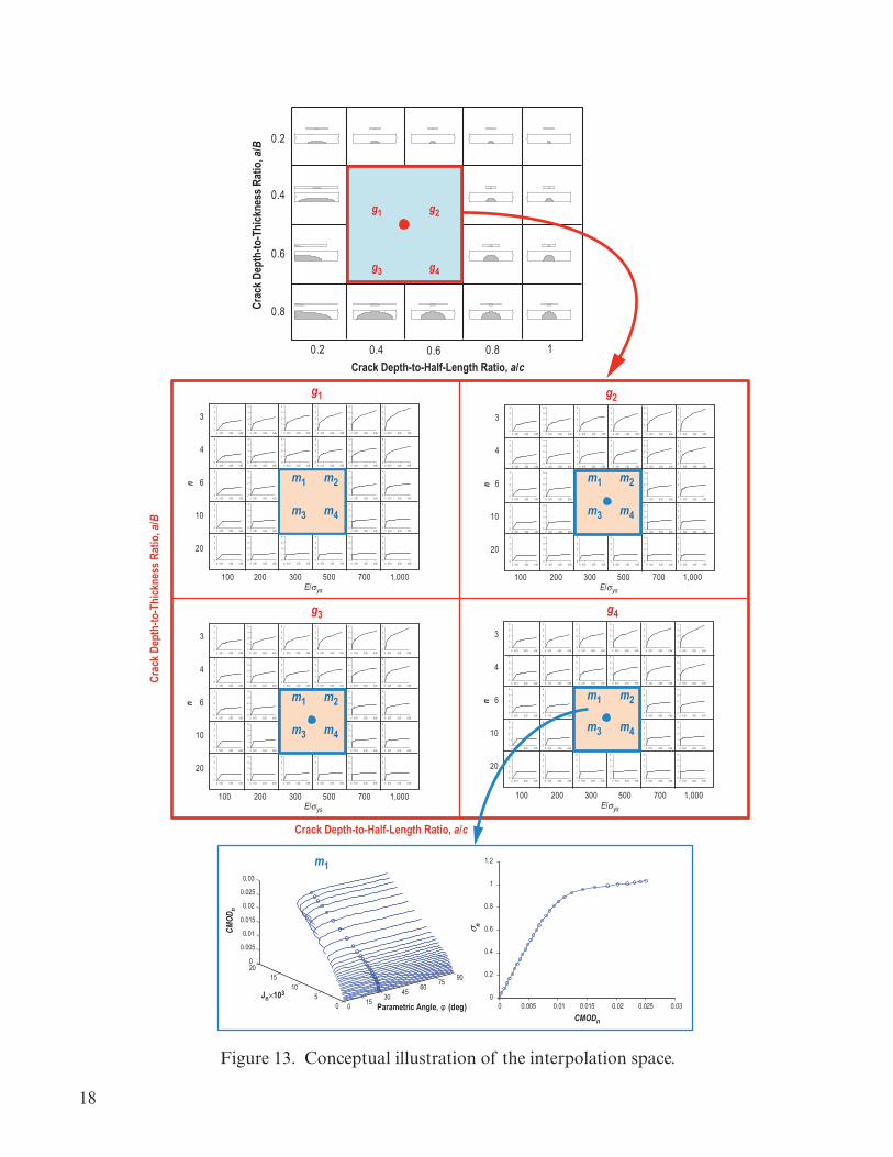
The methodology for setting uniform spacing and magnitude for loading conditions across the 16 subset solutions is not as straightforward. Since the FEMs are run to different levels of sn and CMODn, several choices must be made concerning how to divide the solutions into load incre-ments including: the measure used for parsing (sn or CMODn), the load increment spacing, and a method to either truncate or extend the solutions. As stated above, the authors chose to use CMODn as the parsing measure of loading condition, thus a common maximum value of CMODn across all 16 sets is needed. Figure 14(a) plots sn versus CMODn for the 16 subset solutions and illustrates the challenge in determining the maximum allowed CMODn value for the solution set. The minimum, maximum, and average CMODn values are designated by vertical lines in figure 14(a). Truncating all of the data sets to the minimum CMODn of the 16 sets severely limits the extent of the solutions. In turn, extrapolating all of the data sets out to the maximum CMODn value requires extending some solutions to CMODn values far beyond their final converged load increment. Instead, the authors chose to set the maximum common loading condition equal to the average CMODn of the 16 data sets. Solutions that extend beyond the average CMODn are truncated. Solutions with maximum CMODn values less than the average are extrapolated out to the average CMODn by fitting a power law of the form sn=α*(CMODn)β+γ to the last five sn versus CMODn data points in the set, where α,β,and γ are fitting constants. Once the 16 data sets have all been either truncated or extrapolated to the same maximum CMODn, each set is divided into 20 even CMODn increments common across all sets. Linear interpolation is used to determine the values of sn for the 20 CMODn increments. Figure 14(b) illustrates the 16 sn versus CMODn data sets with 20 even CMODn increments out to the average CMODn.

20

0 0.005 0.01 0.015 0.02 0.025 0.03 0.035 0.04 0.0450

0.5

1

1.5

1.5

CMODn

CMODnCMODn

0 0.005 0.01 0.015 0.02 0.025 0.03 0.035 0.04 0.0450

0.5

1

(b)

(a)

FEM DataMinimum CMODMaximum CMODAverage CMOD


Nor

mali

zed

Far-F

ield

Stre

ss, σ

n N

orm

alize

d Fa

r-Fiel

d St

ress

, σn

Figure 14. Illustration of (a) effect of truncating the solution space based on the average of the maximum CMODn values on the sn versus CMODn results, and (b) dividing the CMODn into even incre-ments for sn versus CMODn interpolation.

21

With each of the 16 subset solutions adjusted to common increments of CMODn, the Jn(f) values for the new load increments must be interpolated. Figure 15(a) shows Jn(f = 90°) versus CMODn for the same 16 subsets shown in figure 14. The Jn versus CMODn solutions that extended beyond the average CMODn are truncated while the solutions that are less than the average CMODn are extrapolated using linear extrapolation. Linear extrapolation works well for these data because the Jn versus CMODn response becomes approximately linear once into the elastic-plastic regime. Figure 15(b) illustrates Jn(f = 90°) versus CMODn data sets with 20 even CMODn increments out to the average CMODn.

22

0 0.005 0.01 0.015 0.02 0.025 0.03 0.035 0.04 0.0450

5

10

15

20

25

30

0 0.005 0.01 0.015 0.02 0.025 0.03 0.035 0.04 0.0450

5

10

15

20

25

30

J n (φ

= 90)

× 10

3J n

(φ= 9

0) ×

103

CMODn

CMODn



(b)

(a)

Figure 15. Illustration of (a) effect of truncating the solution space based on the average of the maximum CMODn values on the Jn versus CMODn results, and (b) dividing the CMODn into even incre-ments for Jn versus CMODn interpolation.

23

Once the 16 subset solutions are prepared with even f spacing and load increments, the step-by-step interpolation process to the final R can proceed. Figure 16 illustrates the four-step interpolation process used by the authors. Each of the steps are indicated by the Roman numerals I through IV. At each interpolation step I through IV, Jn is interpolated at each f location for each CMODn increment to determine a new Jn(f) versus CMODn. A second interpolation process evalu-ates sn for each CMODn increment. Step I in the interpolation process begins with the 16 prepared subset solutions for linear interpolation based on crack shape ratio, a/c. Within the 16 solutions, there are eight pairs of solutions that differ only by a/c. Linear interpolation occurs between these pairs based on the target a/c value, resulting in eight new solutions, all with the same a/c value but different combinations of a/B, n, and E/sys. In step II, linear interpolation is performed on the four pairs of solutions that differ only by crack depth, a/B, to the chosen a/B value for R . This results in four new solutions with the same geometric values but different material values. In step III, two pairs of solutions are linearly interpolated in terms of n to the chosen n value for R resulting in two new solutions differing only in their E/sys values. Finally, in step IV, the remaining two solutions are interpolated to the chosen E/sys, resulting in the final R interpolated solution. As will be shown in section 3, the Jn(f) and sn values have nonlinear spacing with E/sys; therefore, for the step IV inter-polation, linear interpolation was performed in terms of log10(E/sys) and the log10 of the chosen E/sys for R value.

24

0 0.01 0.03 0.050

1

2

3

4

0 0.01 0.03 0.050

1

2

3

4

0 0.01 0.03 0.050

1

2

3

4

0 0.01 0.03 0.050

1

2

3

4

0 0.01 0.03 0.050

1

2

3

4

0 0.01 0.03 0.050

1

2

3

4

0 0.01 0.03 0.050

1

2

3

4

0 0.01 0.03 0.050

1

2

3

4

0 0.01 0.03 0.050

1

2

3

4

0 0.01 0.03 0.050

1

2

3

4

0 0.01 0.03 0.050

1

2

3

4

0 0.01 0.03 0.050

1

2

3

4

0 0.01 0.03 0.050

1

2

3

4

0 0.01 0.03 0.050

1

2

3

4

0 0.01 0.03 0.050

1

2

3

4

0 0.01 0.03 0.050

1

2

3

4

0 0.01 0.03 0.050

1

2

3

4

0 0.01 0.03 0.050

1

2

3

4

0 0.01 0.03 0.050

1

2

3

4

0 0.01 0.03 0.050

1

2

3

4

0 0.01 0.03 0.050

1

2

3

4

0 0.01 0.03 0.050

1

2

3

4

0 0.01 0.03 0.050

1

2

3

4

0 0.01 0.03 0.050

1

2

3

4

0 0.01 0.03 0.050

1

2

3

4

0 0.01 0.03 0.050

1

2

3

4

0 0.01 0.03 0.050

1

2

3

4

0 0.01 0.03 0.050

1

2

3

4

0 0.01 0.03 0.050

1

2

3

4

0 0.01 0.03 0.050

1

2

3

4

20

10

6

4

3

100 200 300 500 700 1000E / ys

0 0.01 0.03 0.050

1

2

3

4

0 0.01 0.03 0.050

1

2

3

4

0 0.01 0.03 0.050

1

2

3

4

0 0.01 0.03 0.050

1

2

3

4

0 0.01 0.03 0.050

1

2

3

4

0 0.01 0.03 0.050

1

2

3

4

0 0.01 0.03 0.050

1

2

3

4

0 0.01 0.03 0.050

1

2

3

4

0 0.01 0.03 0.050

1

2

3

4

0 0.01 0.03 0.050

1

2

3

4

0 0.01 0.03 0.050

1

2

3

4

0 0.01 0.03 0.050

1

2

3

4

0 0.01 0.03 0.050

1

2

3

4

0 0.01 0.03 0.050

1

2

3

4

0 0.01 0.03 0.050

1

2

3

4

0 0.01 0.03 0.050

1

2

3

4

0 0.01 0.03 0.050

1

2

3

4

0 0.01 0.03 0.050

1

2

3

4

0 0.01 0.03 0.050

1

2

3

4

0 0.01 0.03 0.050

1

2

3

4

0 0.01 0.03 0.050

1

2

3

4

0 0.01 0.03 0.050

1

2

3

4

0 0.01 0.03 0.050

1

2

3

4

0 0.01 0.03 0.050

1

2

3

4

0 0.01 0.03 0.050

1

2

3

4

0 0.01 0.03 0.050

1

2

3

4

0 0.01 0.03 0.050

1

2

3

4

0 0.01 0.03 0.050

1

2

3

4

0 0.01 0.03 0.050

1

2

3

4

0 0.01 0.03 0.050

1

2

3

4

20

10

6

4

3

100 200 300 500 700 1000

n

E / ys

0 0.01 0.03 0.050

1

2

3

4

0 0.01 0.03 0.050

1

2

3

4

0 0.01 0.03 0.050

1

2

3

4

0 0.01 0.03 0.050

1

2

3

4

0 0.01 0.03 0.050

1

2

3

4

0 0.01 0.03 0.050

1

2

3

4

0 0.01 0.03 0.050

1

2

3

4

0 0.01 0.03 0.050

1

2

3

4

0 0.01 0.03 0.050

1

2

3

4

0 0.01 0.03 0.050

1

2

3

4

0 0.01 0.03 0.050

1

2

3

4

0 0.01 0.03 0.050

1

2

3

4

0 0.01 0.03 0.050

1

2

3

4

0 0.01 0.03 0.050

1

2

3

4

0 0.01 0.03 0.050

1

2

3

4

0 0.01 0.03 0.050

1

2

3

4

0 0.01 0.03 0.050

1

2

3

4

0 0.01 0.03 0.050

1

2

3

4

0 0.01 0.03 0.050

1

2

3

4

0 0.01 0.03 0.050

1

2

3

4

0 0.01 0.03 0.050

1

2

3

4

0 0.01 0.03 0.050

1

2

3

4

0 0.01 0.03 0.050

1

2

3

4

0 0.01 0.03 0.050

1

2

3

4

0 0.01 0.03 0.050

1

2

3

4

0 0.01 0.03 0.050

1

2

3

4

0 0.01 0.03 0.050

1

2

3

4

0 0.01 0.03 0.050

1

2

3

4

0 0.01 0.03 0.050

1

2

3

4

0 0.01 0.03 0.050

1

2

3

4

20

10

6

4

3

100 200 300 500 700 1000E / ys

0 0.01 0.03 0.050

1

2

3

4

0 0.01 0.03 0.050

1

2

3

4

0 0.01 0.03 0.050

1

2

3

4

0 0.01 0.03 0.050

1

2

3

4

0 0.01 0.03 0.050

1

2

3

4

0 0.01 0.03 0.050

1

2

3

4

0 0.01 0.03 0.050

1

2

3

4

0 0.01 0.03 0.050

1

2

3

4

0 0.01 0.03 0.050

1

2

3

4

0 0.01 0.03 0.050

1

2

3

4

0 0.01 0.03 0.050

1

2

3

4

0 0.01 0.03 0.050

1

2

3

4

0 0.01 0.03 0.050

1

2

3

4

0 0.01 0.03 0.050

1

2

3

4

0 0.01 0.03 0.050

1

2

3

4

0 0.01 0.03 0.050

1

2

3

4

0 0.01 0.03 0.050

1

2

3

4

0 0.01 0.03 0.050

1

2

3

4

0 0.01 0.03 0.050

1

2

3

4

0 0.01 0.03 0.050

1

2

3

4

0 0.01 0.03 0.050

1

2

3

4

0 0.01 0.03 0.050

1

2

3

4

0 0.01 0.03 0.050

1

2

3

4

0 0.01 0.03 0.050

1

2

3

4

0 0.01 0.03 0.050

1

2

3

4

0 0.01 0.03 0.050

1

2

3

4

0 0.01 0.03 0.050

1

2

3

4

0 0.01 0.03 0.050

1

2

3

4

0 0.01 0.03 0.050

1

2

3

4

0 0.01 0.03 0.050

1

2

3

4

20

10

6

4

3

100 200 300 500 700 1000

n

E / ys

0 0.01 0.03 0.050

1

2

3

4

0 0.01 0.03 0.050

1

2

3

4

0 0.01 0.03 0.050

1

2

3

4

0 0.01 0.03 0.050

1

2

3

4

0 0.010

1

2

3

4

0 0.01 0.03 0.050

1

2

3

4

0 0.01 0.03 0.050

1

2

3

4

0 0.01 0.03 0.050

1

2

3

4

0 0.01 0.03 0.050

1

2

3

4

0 0.010

1

2

3

4

0 0.01 0.03 0.050

1

2

3

4

0 0.01 0.03 0.050

1

2

3

4

0 0.01 0.03 0.050

1

2

3

4

0 0.01 0.03 0.050

1

2

3

4

0 0.010

1

2

3

4

0 0.01 0.03 0.050

1

2

3

4

0 0.01 0.03 0.050

1

2

3

4

0 0.01 0.03 0.050

1

2

3

4

0 0.01 0.03 0.050

1

2

3

4

0 0.010

1

2

3

4

0 0.01 0.03 0.050

1

2

3

4

0 0.01 0.03 0.050

1

2

3

4

0 0.01 0.03 0.050

1

2

3

4

0 0.01 0.03 0.050

1

2

3

4

0 0.010

1

2

3

4

20

10

6

4

3

100 200 300 500

n

E / ys

0 0.01 0.03 0.050

1

2

3

4

0 0.01 0.03 0.050

1

2

3

4

0 0.01 0.03 0.050

1

2

3

4

0 0.01 0.03 0.050

1

2

3

4

0 0.010

1

2

3

4

0 0.01 0.03 0.050

1

2

3

4

0 0.01 0.03 0.050

1

2

3

4

0 0.01 0.03 0.050

1

2

3

4

0 0.01 0.03 0.050

1

2

3

4

0 0.010

1

2

3

4

0 0.01 0.03 0.050

1

2

3

4

0 0.01 0.03 0.050

1

2

3

4

0 0.01 0.03 0.050

1

2

3

4

0 0.01 0.03 0.050

1

2

3

4

0 0.010

1

2

3

4

0 0.01 0.03 0.050

1

2

3

4

0 0.01 0.03 0.050

1

2

3

4

0 0.01 0.03 0.050

1

2

3

4

0 0.01 0.03 0.050

1

2

3

4

0 0.010

1

2

3

4

0 0.01 0.03 0.050

1

2

3

4

0 0.01 0.03 0.050

1

2

3

4

0 0.01 0.03 0.050

1

2

3

4

0

1

2

3

4

20

10

6

4

3

100 200 300 500

n

E / ys

0 1530

4560

7590

05

1015

200

0.005

0.01

0.015

0.02

0.025

0.03

CMOD

n

0 0.005 0.01 0.015 0.02 0.025 0.030

0.2

0.4

0.6

0.8

1

1.2

CMODn

Jn×103Parametric Angle, φ (deg)

σ n

m1 m2

m3 m4

m1 m2

m3 m4

m1 m2

m3 m4

m1 m2

m3 m4

m1 m2

m3 m4

m1

m1

m1,3 m2,4

m2

m3 m4

m2

m3 m4

g1g1,2

g3,4

g1,2 – 3,4

g1,2 – 3,4 m1,3 – 2,4

g1,2 – 3,4

g2

g3 g4

Step I — a/c Interpolation Step II — a/B Interpolation

Step III — n Interpolation Step IV — E / ys Interpolationσ

Final — R (a/B, a/c, n, E / ys) σ

Figure 16. Conceptual illustration of the interpolation process. Arrow indicates interpolation direction.

25

Figures 17–20 illustrate the interpolation steps I through IV, respectively, for the example interpolated solution,

R a / B,a / c,n,E / σ ys( ) = R 0.5,0.5,8,400( ) . Each figure shows a comparison of

results for: (1) sn versus CMODn, (2) Jn(f = 90°) versus CMODn, and (3) Jn(f) for the final common loading condition of the nearest neighbor solution subsets along with the final interpolated result, R . The solution subset results are plotted as solid lines with open symbols; the open symbols repre-sent specific materials (m1–m4 in figs. 13 and 16) while the colors represent specific geometry choices (g1–g4 in figs. 13 and 16). The final interpolated results are plotted with a solid line with filled star-shaped symbols. Figure 17 represents the original 16 subsets prior to step I interpolation process on a/c. Figure 18 shows the resulting eight solutions of step I prior to the step II interpolation for a/B. Figure 19 shows the resulting four solutions of step II prior to step III interpolation on the n value. Lastly, figure 20 shows the final two solutions to be interpolated by E/sys in step IV.

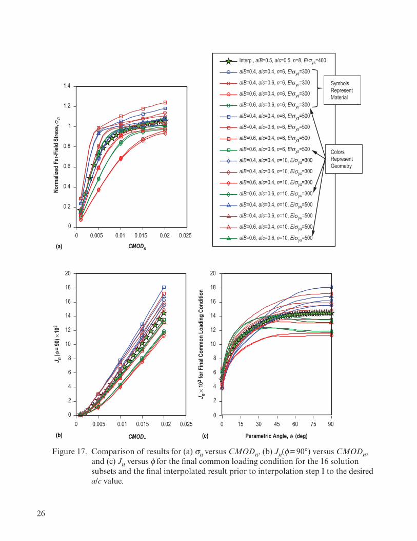
26

0 0.005 0.01 0.015 0.02 0.0250

0.2

0.4

0.6

0.8

1

1.2

1.4

Interp., a/B=0.5, a/c=0.5, n=8, E/ ys=400

a/B=0.4, a/c=0.4, n=6, E/ ys=300

a/B=0.4, a/c=0.6, n=6, E/ ys=300

a/B=0.6, a/c=0.4, n=6, E/ ys=300

a/B=0.6, a/c=0.6, n=6, E/ ys=300

a/B=0.4, a/c=0.4, n=6, E/ ys=500

a/B=0.4, a/c=0.6, n=6, E/ ys=500

a/B=0.6, a/c=0.4, n=6, E/ ys=500

a/B=0.6, a/c=0.6, n=6, E/ ys=500

a/B=0.4, a/c=0.4, n=10, E/ ys=300

a/B=0.4, a/c=0.6, n=10, E/ ys=300

a/B=0.6, a/c=0.4, n=10, E/ ys=300

a/B=0.6, a/c=0.6, n=10, E/ ys=300

a/B=0.4, a/c=0.4, n=10, E/ ys=500

a/B=0.4, a/c=0.6, n=10, E/ ys=500

a/B=0.6, a/c=0.4, n=10, E/ ys=500

a/B=0.6, a/c=0.6, n=10, E/ ys=500

0 0.005 0.01 0.015 0.02 0.0250

2

4

6

8

10

12

14

16

18

20

CMODn

CMODn

0 15 30 45 60 75 900

2

4

6

8

10

12

14

16

18

20


(a)

(b) (c)

J n (φ

= 90)

× 10

3

J n ×

103 f

or F

inal

Com

mon

Loa

ding

Con

ditio

n

SymbolsRepresentMaterial

ColorsRepresentGeometry

σ

σ

σ

σ

σ

σ

σ

σ

σ

σ

σ

σ

σ

σ

σ

σ

σ

Norm

alize

d Fa

r-Fiel

d St

ress

, n

σ

Figure 17. Comparison of results for (a) sn versus CMODn, (b) Jn(f = 90°) versus CMODn, and (c) Jn versus f for the final common loading condition for the 16 solution subsets and the final interpolated result prior to interpolation step I to the desired a/c value.

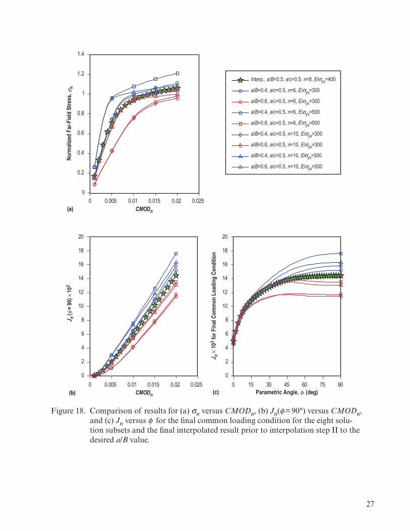
27

0 0.005 0.01 0.015 0.02 0.0250

0.2

0.4

0.6

0.8

1

1.2

1.4

Interp., a/B=0.5, a/c=0.5, n=8, E/ ys=400

a/B=0.4, a/c=0.5, n=6, E/ ys=300

a/B=0.6, a/c=0.5, n=6, E/ ys=300

a/B=0.4, a/c=0.5, n=6, E/ ys=500

a/B=0.6, a/c=0.5, n=6, E/ ys=500

a/B=0.4, a/c=0.5, n=10, E/ ys=300

a/B=0.6, a/c=0.5, n=10, E/ ys=300

a/B=0.4, a/c=0.5, n=10, E/ ys=500

a/B=0.6, a/c=0.5, n=10, E/ ys=500

0 0.005 0.01 0.015 0.02 0.0250

2

4

6

8

10

12

14

16

18

20

0 15 30 45 60 75 900

2

4

6

8

10

12

14

16

18

20

(a)

(b) (c)

CMODn

CMODn

J n (φ

= 90)

× 10

3

σ

σ

σ

σ

σ

σ

σ

σ

σ


Norm

alize

d Fa

r-Fiel

d St

ress

, n σ

J n ×

103 f

or F

inal

Com

mon

Loa

ding

Con

ditio

n

Figure 18. Comparison of results for (a) sn versus CMODn, (b) Jn(f = 90°) versus CMODn, and (c) Jn versus f for the final common loading condition for the eight solu-tion subsets and the final interpolated result prior to interpolation step II to the desired a/B value.

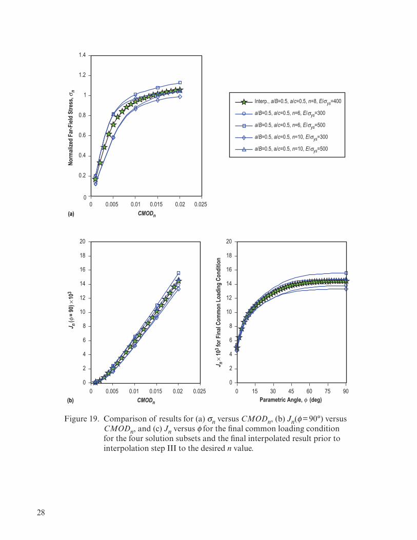
28

0 0.005 0.01 0.015 0.02 0.0250

0.2

0.4

0.6

0.8

1

1.2

1.4

Interp., a/B=0.5, a/c=0.5, n=8, E/ ys=400

a/B=0.5, a/c=0.5, n=6, E/ ys=300

a/B=0.5, a/c=0.5, n=6, E/ ys=500

a/B=0.5, a/c=0.5, n=10, E/ ys=300

a/B=0.5, a/c=0.5, n=10, E/ ys=500

0 0.005 0.01 0.015 0.02 0.0250

2

4

6

8

10

12

14

16

18

20

0 15 30 45 60 75 900

2

4

6

8

10

12

14

16

18

20

(a)

(b)

CMODn

σ

σ

σ

σ

σ

J n (φ

= 90)

× 10

3

CMODn Parametric Angle, φ (deg)

Norm

alize

d Fa

r-Fiel

d St

ress

, n σ

J n ×

103 f

or F

inal

Com

mon

Loa

ding

Con

ditio

n

Figure 19. Comparison of results for (a) sn versus CMODn, (b) Jn(f = 90°) versus CMODn, and (c) Jn versus f for the final common loading condition for the four solution subsets and the final interpolated result prior to interpolation step III to the desired n value.

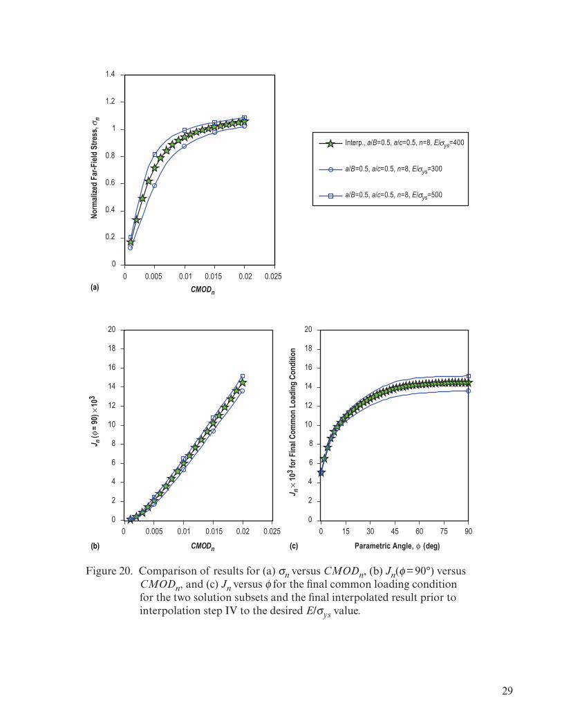
29

0 0.005 0.01 0.015 0.02 0.0250

0.2

0.4

0.6

0.8

1

1.2

1.4

Interp., a/B=0.5, a/c=0.5, n=8, E/ ys=400

a/B=0.5, a/c=0.5, n=8, E/ ys=300

a/B=0.5, a/c=0.5, n=8, E/ ys=500

0 0.005 0.01 0.015 0.02 0.0250

2

4

6

8

10

12

14

16

18

20

0 15 30 45 60 75 900

2

4

6

8

10

12

14

16

18

20

(a)

(b) (c) CMODn

CMODn


J n (φ

= 90)

× 10

3

σ

σ

σ

Norm

alize

d Fa

r-Fiel

d St

ress

, n σ

J n ×

103 f

or F

inal

Com

mon

Loa

ding

Con

ditio

n

Figure 20. Comparison of results for (a) sn versus CMODn, (b) Jn(f = 90°) versus CMODn, and (c) Jn versus f for the final common loading condition for the two solution subsets and the final interpolated result prior to interpolation step IV to the desired E/sys value.

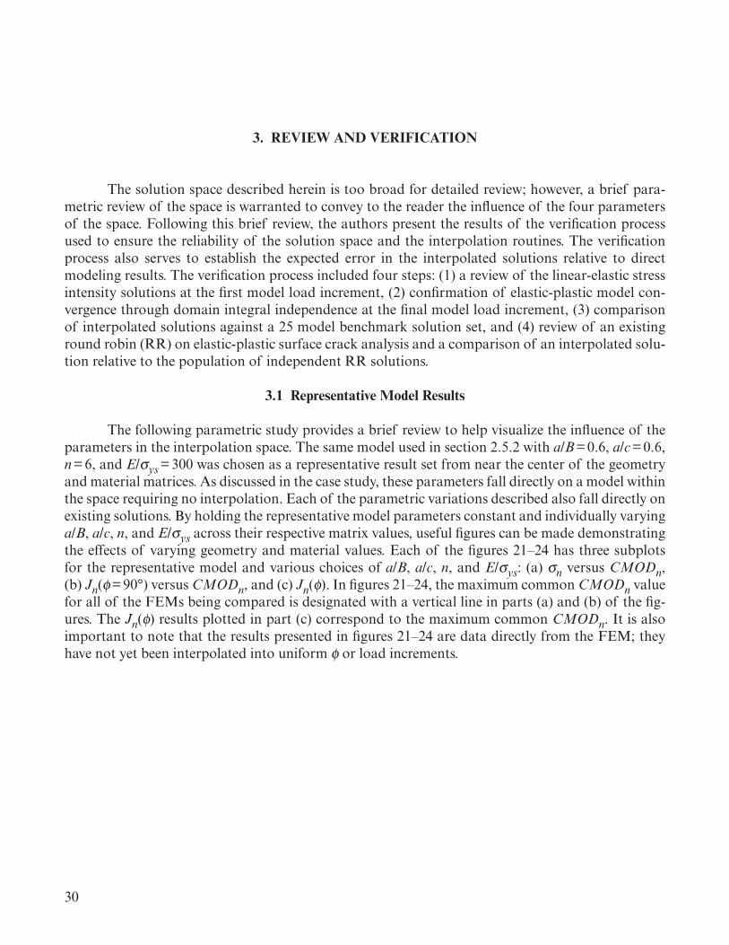
30

3. REVIEW AND VERIFICATION

The solution space described herein is too broad for detailed review; however, a brief para-metric review of the space is warranted to convey to the reader the influence of the four parameters of the space. Following this brief review, the authors present the results of the verification process used to ensure the reliability of the solution space and the interpolation routines. The verification process also serves to establish the expected error in the interpolated solutions relative to direct modeling results. The verification process included four steps: (1) a review of the linear-elastic stress intensity solutions at the first model load increment, (2) confirmation of elastic-plastic model con-vergence through domain integral independence at the final model load increment, (3) comparison of interpolated solutions against a 25 model benchmark solution set, and (4) review of an existing round robin (RR) on elastic-plastic surface crack analysis and a comparison of an interpolated solu-tion relative to the population of independent RR solutions.

3.1 Representative Model Results

The following parametric study provides a brief review to help visualize the influence of the parameters in the interpolation space. The same model used in section 2.5.2 with a/B = 0.6, a/c = 0.6, n = 6, and E/sys = 300 was chosen as a representative result set from near the center of the geometry and material matrices. As discussed in the case study, these parameters fall directly on a model within the space requiring no interpolation. Each of the parametric variations described also fall directly on existing solutions. By holding the representative model parameters constant and individually varying a/B, a/c, n, and E/sys across their respective matrix values, useful figures can be made demonstrating the effects of varying geometry and material values. Each of the figures 21–24 has three subplots for the representative model and various choices of a/B, a/c, n, and E/sys: (a) sn versus CMODn, (b) Jn(f= 90°)versus CMODn, and (c) Jn(f). In figures 21–24, the maximum common CMODn value for all of the FEMs being compared is designated with a vertical line in parts (a) and (b) of the fig-ures. The Jn(f) results plotted in part (c) correspond to the maximum common CMODn. It is also important to note that the results presented in figures 21–24 are data directly from the FEM; they have not yet been interpolated into uniform f or load increments.

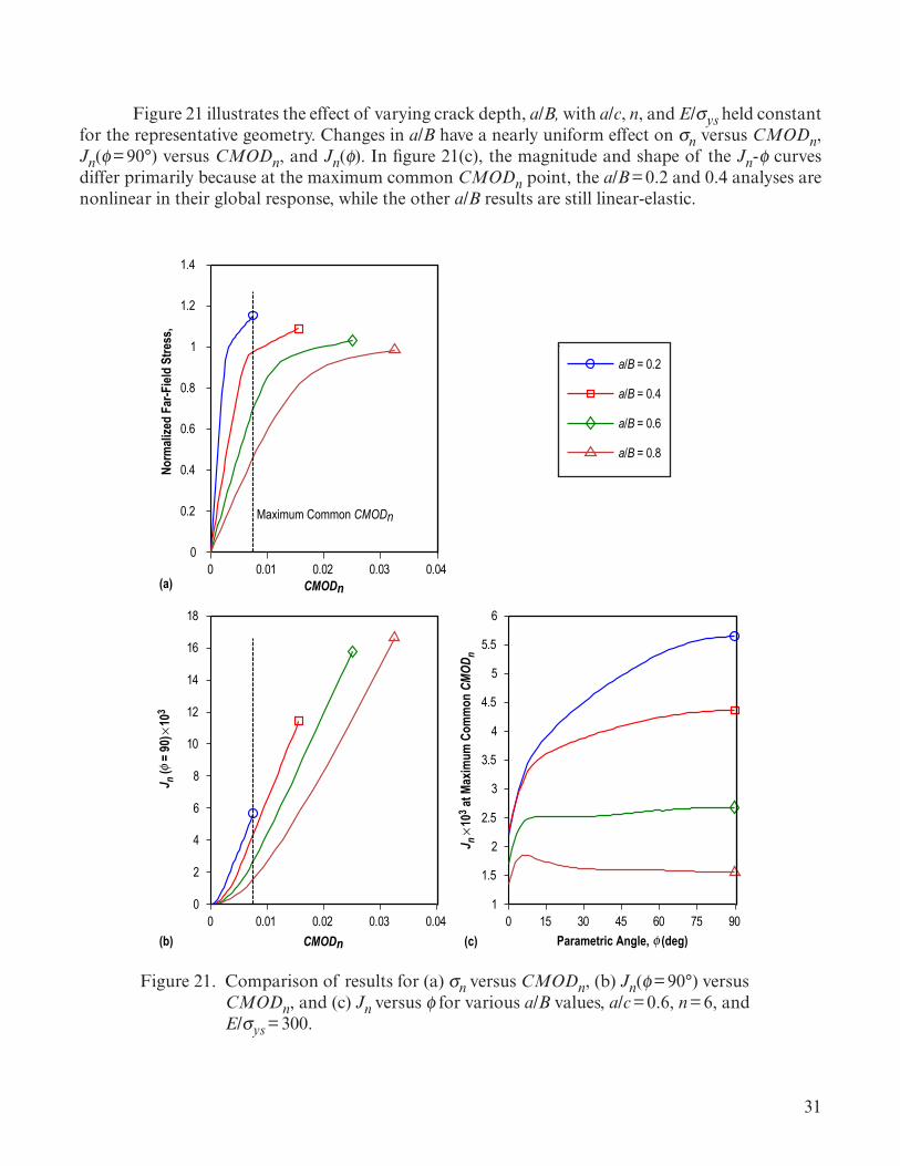
31

Figure 21 illustrates the effect of varying crack depth, a/B, with a/c, n, and E/sys held constant for the representative geometry. Changes in a/B have a nearly uniform effect on sn versus CMODn, Jn(f= 90°) versus CMODn, and Jn(f).In figure 21(c), the magnitude and shape of the Jn- f curves differ primarily because at the maximum common CMODn point, the a/B = 0.2 and 0.4 analyses are nonlinear in their global response, while the other a/B results are still linear-elastic.

0 0.01 0.02 0.03 0.040

0.2

0.4

0.6

0.8

1

1.2

1.4

a/B = 0.2

a/B = 0.4

a/B = 0.6

a/B = 0.8

0 0.01 0.02 0.03 0.040

2

4

6

8

10

12

14

16

18

0 15 30 45 60 75 901

1.5

2

2.5

3

3.5

4

4.5

5

5.5

6

Parametric Angle, (deg)CMODn

CMODn

Maximum Common CMODn

Norm

alize

d Fa

r-Fiel

d St

ress

,J n (

= 90

)×10

3

J n ×1

03 at M

axim

um C

omm

on C

MOD n

φ

φ

(a)

(b) (c)

Figure 21. Comparison of results for (a) sn versus CMODn, (b) Jn(f = 90°) versus CMODn, and (c) Jn versus f for various a/B values, a/c = 0.6, n = 6, and E/sys = 300.

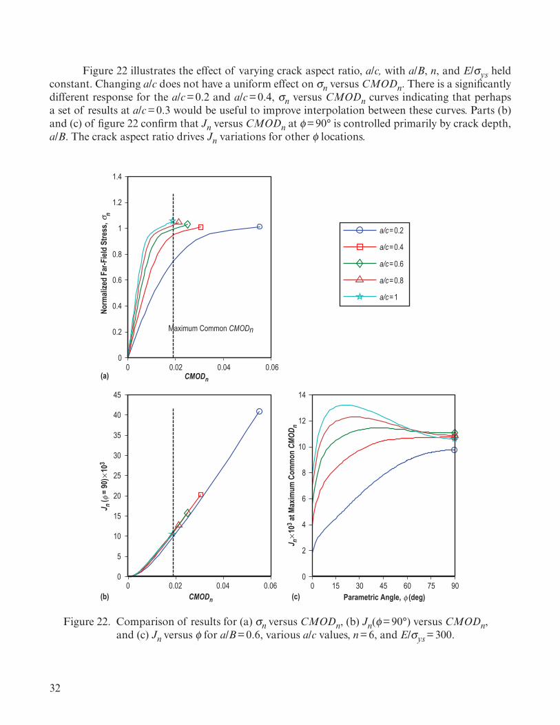
32

Figure 22 illustrates the effect of varying crack aspect ratio, a/c, with a/B, n, and E/sys held constant. Changing a/c does not have a uniform effect on sn versus CMODn. There is a significantly different response for the a/c = 0.2 and a/c = 0.4, sn versus CMODn curves indicating that perhaps a set of results at a/c = 0.3 would be useful to improve interpolation between these curves. Parts (b) and (c) of figure 22 confirm that Jn versus CMODn at f = 90° is controlled primarily by crack depth, a/B. The crack aspect ratio drives Jn variations for other f locations.

0 0.02 0.04 0.06

a/c=0.2

a/c=0.4

a/c=0.6

a/c=0.8

a/c=1

0 0.02 0.04 0.060

5

10

15

20

25

30

35

40

45

0

2

4

6

8

10

12

14

J n (

= 90

)×10

3

(a)

(b) (c) Parametric Angle, (deg)φ

0

0.2

0.4

0.6

0.8

1

1.2

1.4

0 15 30 45 60 75 90CMODn

CMODn

φ


Norm

alize

d Fa

r-Fiel

d St

ress

,n

J n×10

3 at M

axim

um C

omm

on C

MOD n

σ

Figure 22. Comparison of results for (a) sn versus CMODn, (b) Jn(f = 90°) versus CMODn, and (c) Jn versus f for a/B = 0.6, various a/c values, n = 6, and E/sys = 300.

33

Figure 23 illustrates the effect of varying strain hardening exponent, n, with a/B, a/c, and E/sys held constant. As expected, changes in n have no effect on the linear portion of the sn versus CMODn response but do affect the curve once nonlinear. Following directly from the LPPL tensile response, the n = 3 model has the highest sn for a given CMODn while the n = 20 nonlinear response is almost flat and has the lowest sn for a given CMODn. In figure 23(b), the Jn(f= 90°) versus CMODn results are identical for all n values for low deformations in the LEFM regime and then begin to diverge for higher deformations as plasticity increases. Compared to the other parameters, the strain hardening exponent has the weakest effect on the solution space.

0 0.01 0.02 0.03

0 0.01 0.02 0.03

n=3

n=4

n=6

n=10

n=20

0

2

4

6

8

10

12

14

16

18

20

6

8

10

12

14

16

18

(a)


0

0.2

0.4

0.6

0.8

1

1.2

1.4

0 15 30 45 60 75 90CMODn

CMODn

φ


Norm

alize

d Fa

r-Fiel

d St

ress

,n

J n ( =

90)×

103

J n ×1

03 at M

axim

um C

omm

on C

MOD n

σ

Figure 23. Comparison of results for (a) sn versus CMODn, (b) Jn(f = 90°) versus CMODn, and (c) Jn versus f for a/B = 0.6, various n values, and E/sys = 300.

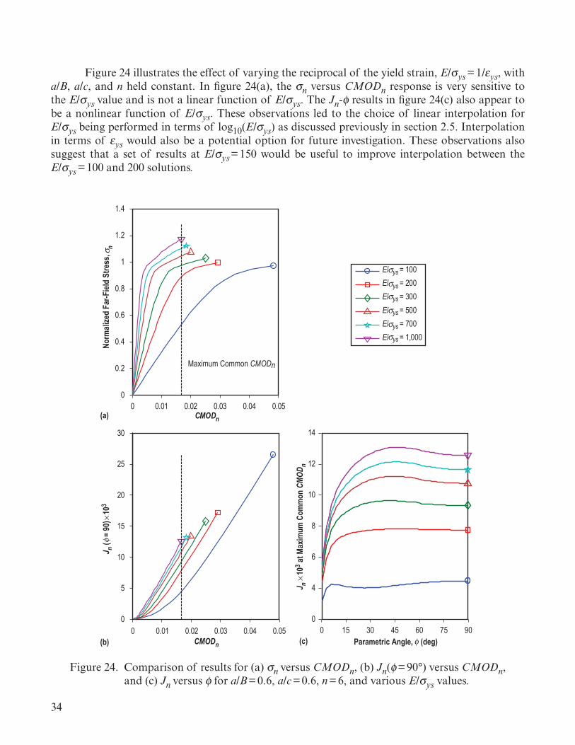
34

Figure 24 illustrates the effect of varying the reciprocal of the yield strain, E/sys = 1/εys, with a/B, a/c, and n held constant. In figure 24(a), the sn versus CMODn response is very sensitive to the E/sys value and is not a linear function of E/sys. The Jn-f results in figure 24(c) also appear to be a nonlinear function of E/sys. These observations led to the choice of linear interpolation for E/sys being performed in terms of log10(E/sys) as discussed previously in section 2.5. Interpolation in terms of εys would also be a potential option for future investigation. These observations also suggest that a set of results at E/sys = 150 would be useful to improve interpolation between the E/sys = 100 and 200 solutions.

4

0

6

8

10

12

14

(a)


0

0.2

0.4

0.6

0.8

1

1.2

1.4

0 15 30 45 60 75 90

E/ = 100E/ = 200E/ = 300E/ = 500E/ = 700E/ ys = 1,000

0 0.01 0.02 0.03 0.04 0.05

0 0.01 0.02 0.03 0.04 0.050

5

10

15

20

25

30

CMODn

CMODn


φJ n (

= 90

)×10

3

J n ×10

3 at M

axim

um C

omm

on C

MOD n

Norm

alize

d Fa

r-Fiel

d St

ress

, nσ

σysσysσysσysσysσ

Figure 24. Comparison of results for (a) sn versus CMODn, (b) Jn(f = 90°) versus CMODn, and (c) Jn versus f for a/B = 0.6, a/c = 0.6, n = 6, and various E/sys values.

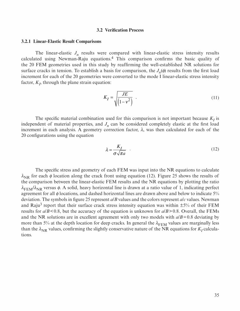
35

3.2 Verification Process

3.2.1 Linear-Elastic Result Comparisons

The linear-elastic Jn results were compared with linear-elastic stress intensity results calculated using Newman-Raju equations.4 This comparison confirms the basic quality of the 20 FEM geometries used in this study by reaffirming the well-established NR solutions for surface cracks in tension. To establish a basis for comparison, the Jn(f) results from the first load increment for each of the 20 geometries were converted to the mode I linear-elastic stress intensity factor, KI, through the plane strain equation:

KI =JE

1− ν2( ) . (11)

The specific material combination used for this comparison is not important because KI is independent of material properties, and Jn can be considered completely elastic at the first load increment in each analysis. A geometry correction factor, λ, was then calculated for each of the 20 configurations using the equation

! =KI

" #a! (12)

The specific stress and geometry of each FEM was input into the NR equations to calculate λNR for each f location along the crack front using equation (12). Figure 25 shows the results of the comparison between the linear-elastic FEM results and the NR equations by plotting the ratio λFEM/λNR versus f. A solid, heavy horizontal line is drawn at a ratio value of 1, indicating perfect agreement for all f locations, and dashed horizontal lines are drawn above and below to indicate 5% deviation. The symbols in figure 25 represent a/B values and the colors represent a/c values. Newman and Raju3 report that their surface crack stress intensity equation was within ±5% of their FEM results for a/B < 0.8, but the accuracy of the equation is unknown for a/B > 0.8. Overall, the FEMs and the NR solutions are in excellent agreement with only two models with a/B = 0.8 deviating by more than 5% at the depth location for deep cracks. In general the λFEM values are marginally less than theλNR values, confirming the slightly conservative nature of the NR equations for KI calcula-tions.

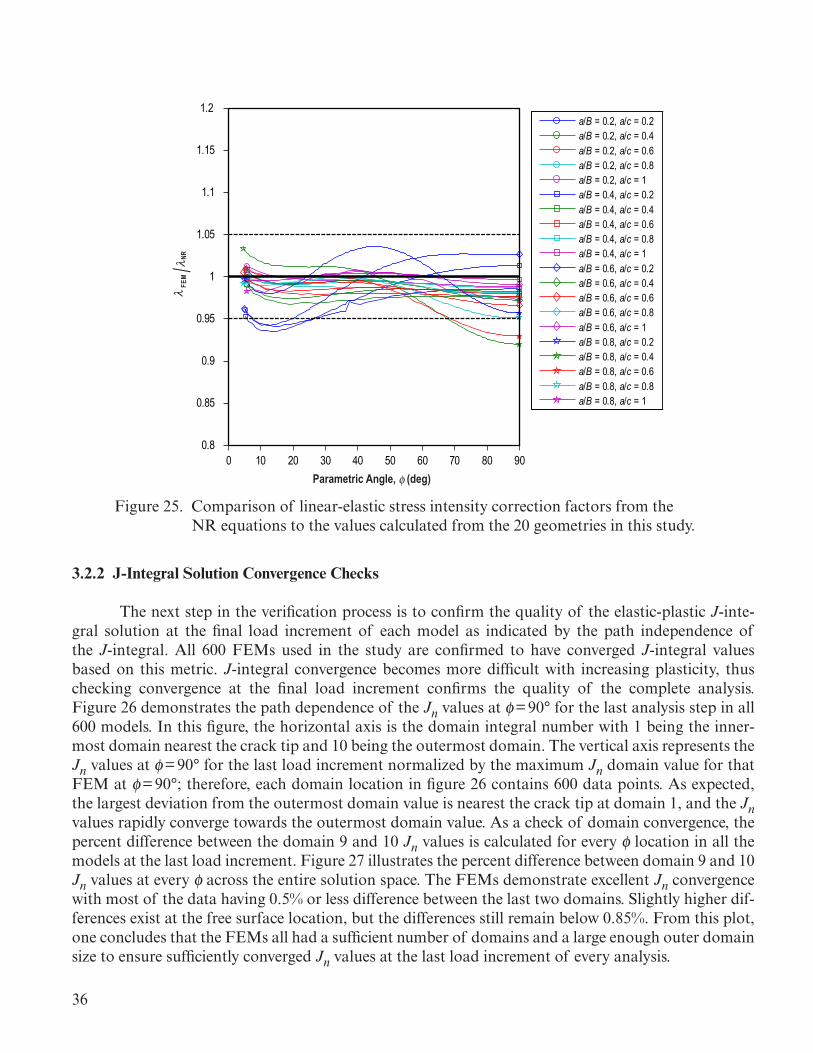
36

0 10 20 30 40 50 60 70 80 900.8

0.85

0.9

0.95

1

1.05

1.1

1.15

1.2a/B = 0.2, a/c = 0.2a/B = 0.2, a/c = 0.4a/B = 0.2, a/c = 0.6a/B = 0.2, a/c = 0.8a/B = 0.2, a/c = 1a/B = 0.4, a/c = 0.2a/B = 0.4, a/c = 0.4a/B = 0.4, a/c = 0.6a/B = 0.4, a/c = 0.8a/B = 0.4, a/c = 1a/B = 0.6, a/c = 0.2a/B = 0.6, a/c = 0.4a/B = 0.6, a/c = 0.6a/B = 0.6, a/c = 0.8a/B = 0.6, a/c = 1a/B = 0.8, a/c = 0.2a/B = 0.8, a/c = 0.4a/B = 0.8, a/c = 0.6a/B = 0.8, a/c = 0.8a/B = 0.8, a/c = 1

Parametric Angle, (deg)φ

FEM / N

R λ

λ

Figure 25. Comparison of linear-elastic stress intensity correction factors from the NR equations to the values calculated from the 20 geometries in this study.

3.2.2 J-Integral Solution Convergence Checks

The next step in the verification process is to confirm the quality of the elastic-plastic J-inte-gral solution at the final load increment of each model as indicated by the path independence of the J-integral. All 600 FEMs used in the study are confirmed to have converged J-integral values based on this metric. J-integral convergence becomes more difficult with increasing plasticity, thus checking convergence at the final load increment confirms the quality of the complete analysis. Figure 26 demonstrates the path dependence of the Jn values at f = 90° for the last analysis step in all 600 models. In this figure, the horizontal axis is the domain integral number with 1 being the inner-most domain nearest the crack tip and 10 being the outermost domain. The vertical axis represents the Jn values at f = 90° for the last load increment normalized by the maximum Jn domain value for that FEM at f= 90°; therefore, each domain location in figure 26 contains 600 data points. As expected, the largest deviation from the outermost domain value is nearest the crack tip at domain 1, and the Jn values rapidly converge towards the outermost domain value. As a check of domain convergence, the percent difference between the domain 9 and 10 Jn values is calculated for every f location in all the models at the last load increment. Figure 27 illustrates the percent difference between domain 9 and 10 Jn values at every f across the entire solution space. The FEMs demonstrate excellent Jn convergence with most of the data having 0.5% or less difference between the last two domains. Slightly higher dif-ferences exist at the free surface location, but the differences still remain below 0.85%. From this plot, one concludes that the FEMs all had a sufficient number of domains and a large enough outer domain size to ensure sufficiently converged Jn values at the last load increment of every analysis.

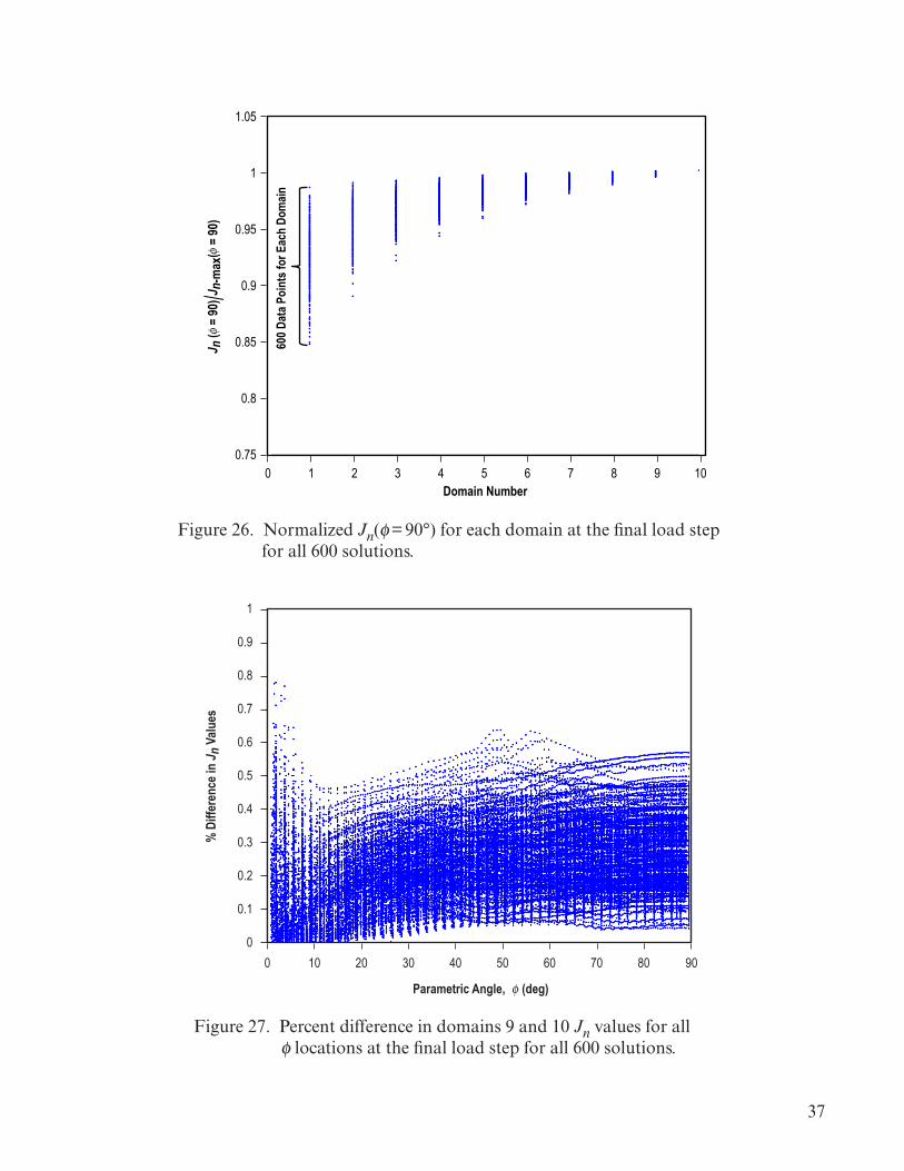
37

0.75

0.8

0.85

0.9

0.95

1

1.05

Domain Number

J n (

= 90

) /J n-m

ax(

= 90

)

600 D

ata P

oint

s for

Eac

h Do

main

φφ

0 1 2 3 4 5 6 7 8 9 10

Figure 26. Normalized Jn(f = 90°) for each domain at the final load step for all 600 solutions.

1

0.9

0.8

0.7

0.6

0.5

0.4

0.3

0.2

0.1

00 10 20 30 40 50 60 70 80 90

(deg)Parametric Angle, φ

% D

iffer

ence

in J n

Valu

es

Figure 27. Percent difference in domains 9 and 10 Jn values for all f locations at the final load step for all 600 solutions.

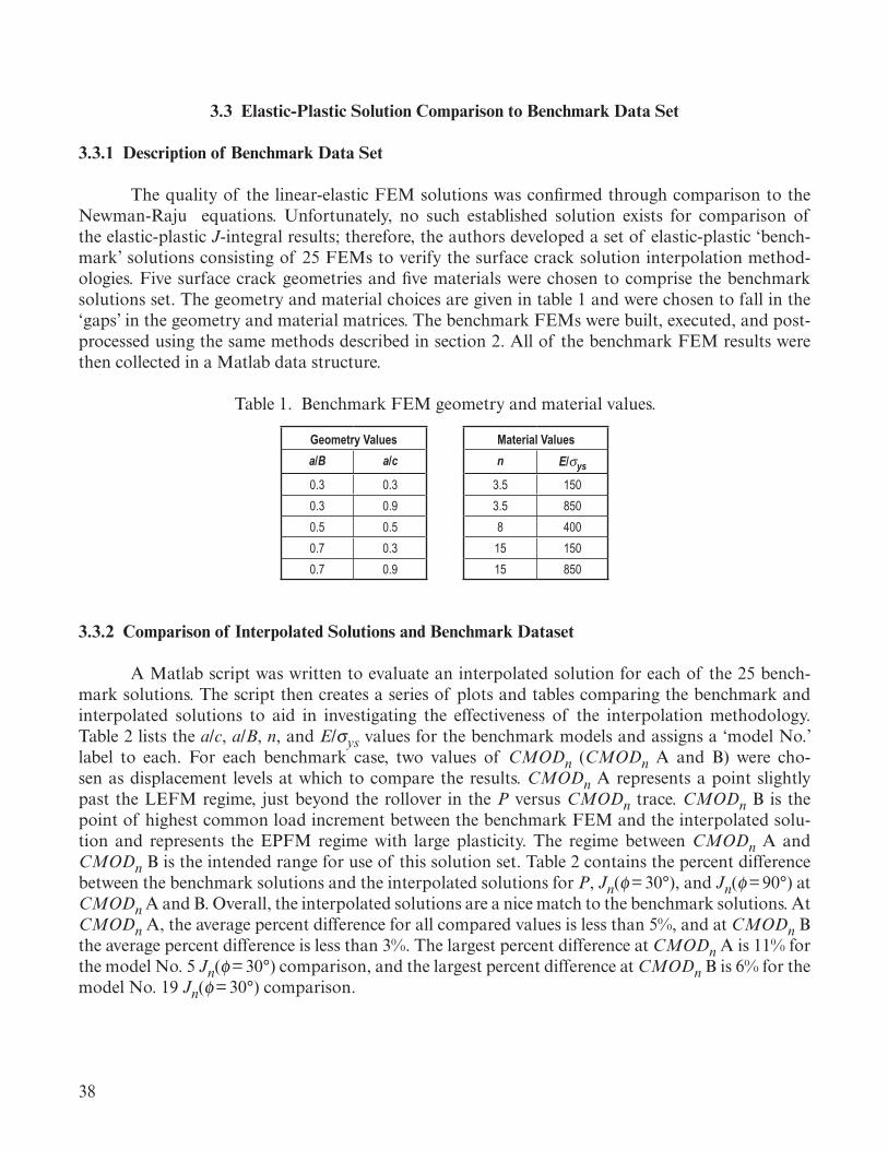
38

3.3 Elastic-Plastic Solution Comparison to Benchmark Data Set

3.3.1 Description of Benchmark Data Set

The quality of the linear-elastic FEM solutions was confirmed through comparison to the Newman-Raju equations. Unfortunately, no such established solution exists for comparison of the elastic-plastic J-integral results; therefore, the authors developed a set of elastic-plastic ‘bench-mark’ solutions consisting of 25 FEMs to verify the surface crack solution interpolation method-ologies. Five surface crack geometries and five materials were chosen to comprise the benchmark solutions set. The geometry and material choices are given in table 1 and were chosen to fall in the ‘gaps’ in the geometry and material matrices. The benchmark FEMs were built, executed, and post-processed using the same methods described in section 2. All of the benchmark FEM results were then collected in a Matlab data structure.

Table 1. Benchmark FEM geometry and material values.

Geometry Values Material Valuesa/B a/c n E/sys

0.3 0.3 3.5 1500.3 0.9 3.5 8500.5 0.5 8 4000.7 0.3 15 1500.7 0.9 15 850

3.3.2 Comparison of Interpolated Solutions and Benchmark Dataset

A Matlab script was written to evaluate an interpolated solution for each of the 25 bench-mark solutions. The script then creates a series of plots and tables comparing the benchmark and interpolated solutions to aid in investigating the effectiveness of the interpolation methodology. Table 2 lists the a/c, a/B, n, and E/sys values for the benchmark models and assigns a ‘model No.’ label to each. For each benchmark case, two values of CMODn (CMODn A and B) were cho-sen as displacement levels at which to compare the results. CMODn A represents a point slightly past the LEFM regime, just beyond the rollover in the P versus CMODn trace. CMODn B is the point of highest common load increment between the benchmark FEM and the interpolated solu-tion and represents the EPFM regime with large plasticity. The regime between CMODn A and CMODn B is the intended range for use of this solution set. Table 2 contains the percent difference between the benchmark solutions and the interpolated solutions for P, Jn(f = 30°), and Jn(f = 90°) at CMODn A and B. Overall, the interpolated solutions are a nice match to the benchmark solutions. At CMODn A, the average percent difference for all compared values is less than 5%, and at CMODn B the average percent difference is less than 3%. The largest percent difference at CMODn A is 11% for the model No. 5 Jn(f = 30°) comparison, and the largest percent difference at CMODn B is 6% for the model No. 19 Jn(f = 30°) comparison.

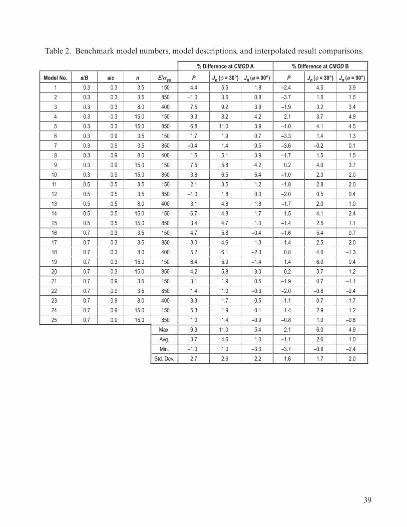
39

Table 2. Benchmark model numbers, model descriptions, and interpolated result comparisons.

% Difference at CMOD A % Difference at CMOD B

Model No. a/B a/c n E/sys P Jn (f = 30°) Jn (f = 90°) P Jn (f = 30°) Jn (f = 90°)1 0.3 0.3 3.5 150 4.4 5.5 1.8 –2.4 4.5 3.92 0.3 0.3 3.5 850 –1.0 3.6 0.8 –3.7 1.5 1.53 0.3 0.3 8.0 400 7.5 9.2 3.9 –1.9 3.2 3.44 0.3 0.3 15.0 150 9.3 8.2 4.2 2.1 3.7 4.95 0.3 0.3 15.0 850 6.8 11.0 3.9 –1.0 4.1 4.56 0.3 0.9 3.5 150 1.7 1.9 0.7 –3.3 1.4 1.37 0.3 0.9 3.5 850 –0.4 1.4 0.5 –3.6 –0.2 0.18 0.3 0.9 8.0 400 1.6 5.1 3.9 –1.7 1.5 1.59 0.3 0.9 15.0 150 7.5 5.8 4.2 0.2 4.0 3.7

10 0.3 0.9 15.0 850 3.8 6.5 5.4 –1.0 2.3 2.011 0.5 0.5 3.5 150 2.1 3.5 1.2 –1.8 2.8 2.012 0.5 0.5 3.5 850 –1.0 1.8 0.0 –2.0 0.5 0.413 0.5 0.5 8.0 400 3.1 4.8 1.8 –1.7 2.0 1.014 0.5 0.5 15.0 150 6.7 4.8 1.7 1.5 4.1 2.415 0.5 0.5 15.0 850 3.4 4.7 1.0 –1.4 2.5 1.116 0.7 0.3 3.5 150 4.7 5.8 –0.4 –1.6 5.4 0.717 0.7 0.3 3.5 850 3.0 4.6 –1.3 –1.4 2.5 –2.018 0.7 0.3 8.0 400 5.2 6.1 –2.3 0.8 4.0 –1.319 0.7 0.3 15.0 150 6.4 5.9 –1.4 1.4 6.0 0.420 0.7 0.3 15.0 850 4.2 5.8 –3.0 0.2 3.7 –1.221 0.7 0.9 3.5 150 3.1 1.9 0.5 –1.9 0.7 –1.122 0.7 0.9 3.5 850 1.4 1.0 –0.3 –2.0 –0.8 –2.423 0.7 0.9 8.0 400 3.3 1.7 –0.5 –1.1 0.7 –1.724 0.7 0.9 15.0 150 5.3 1.9 0.1 1.4 2.9 1.225 0.7 0.9 15.0 850 1.0 1.4 –0.9 –0.8 1.0 –0.8

Max. 9.3 11.0 5.4 2.1 6.0 4.9Avg. 3.7 4.6 1.0 –1.1 2.6 1.0Min. –1.0 1.0 –3.0 –3.7 –0.8 –2.4

Std. Dev. 2.7 2.6 2.2 1.6 1.7 2.0

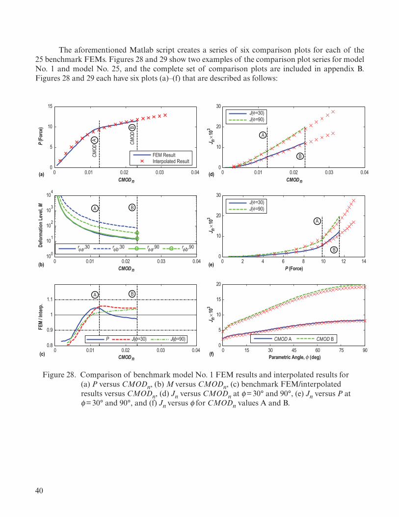
40

The aforementioned Matlab script creates a series of six comparison plots for each of the 25 benchmark FEMs. Figures 28 and 29 show two examples of the comparison plot series for model No. 1 and model No. 25, and the complete set of comparison plots are included in appendix B. Figures 28 and 29 each have six plots (a)–(f) that are described as follows:

0 0.01 0.02 0.03 0.040

5

10

15

P (F

orce

)

FEM ResultInterpolated Result

0 0.01 0.02 0.03 0.040

10

20

30J( =30)J( =90)

0 0.01 0.02 0.03 0.0410

101

0

102

103

104

Defo

rmat

ion

Leve

l, M

r a,30 r b,30 r a,90 r b,90

0 2 4 6 8 10 12 140

10

20

30

P (Force)

0 0.01 0.02 0.03 0.040.8

0.9

1

1.1

CMOD

A

A

A

A

B

B

B

B

n

CMODn

CMOD

CMOD

CMODA

B

n CMODn

FEM

/ Inte

rp.

P J( =30) J( =90)

0 15 30 45 60 75 900

5

10

15

20

J n×1

03J n

×103

J n×1

03

CMOD A CMOD B

(a)

(b)

(c)

(d)

(e)

(f) (deg)Parametric Angle, φ

φ φ φ φ

φφ

J( =30)J( =90)

φφ

φ φ

Figure 28. Comparison of benchmark model No. 1 FEM results and interpolated results for (a) P versus CMODn, (b) M versus CMODn, (c) benchmark FEM/interpolated results versus CMODn, (d) Jn versus CMODn at f = 30° and 90°, (e) Jn versus P at f = 30° and 90°, and (f) Jn versus f for CMODn values A and B.

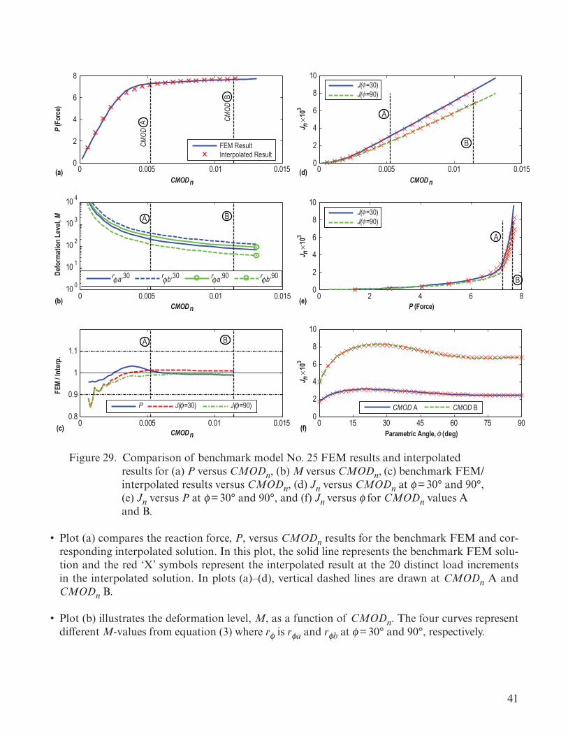
41

P (F

orce

)De

form

atio

n Le

vel, M

P (Force)

CMOD

A

A

B

B

n

CMODn

CMODn CMODn

FEM

/ Inte

rp.

Parametric Angle, (deg)

J n×1

03J n

×103

J n×1

03

(a)

(b)

(c)

(d)

(e)

(f)

0 0.005 0.01 0.0150

2

4

6

8

0 0.005 0.01 0.0150

2

4

6

8

10

0 0.005 0.01 0.01510 0

10 1

10 2

10 3

10 4

0 2 4 6 80

2

4

6

8

10

0 0.005 0.01 0.0150.8

0.9

1

1.1

0 15 30 45 60 75 900

2

4

6

8

10

P J( =30) J( =90) CMOD A CMOD B

φ

J( =30)J( =90)

φφ

φ φ

J( =30)J( =90)

FEM ResultInterpolated Result

CMOD

CMOD

A

B

r a,30 r b,30 r a,90 r b,90

A

A

B

B

B

A

A

B

φφ φ φ

φφ

Figure 29. Comparison of benchmark model No. 25 FEM results and interpolated results for (a) P versus CMODn, (b) M versus CMODn, (c) benchmark FEM/interpolated results versus CMODn, (d) Jn versus CMODn at f = 30° and 90°, (e) Jn versus P at f = 30° and 90°, and (f) Jn versus f for CMODn values A and B.

• Plot (a) compares the reaction force, P, versus CMODn results for the benchmark FEM and cor-responding interpolated solution. In this plot, the solid line represents the benchmark FEM solu-tion and the red ‘X’ symbols represent the interpolated result at the 20 distinct load increments in the interpolated solution. In plots (a)–(d), vertical dashed lines are drawn at CMODn A and CMODn B.

• Plot (b) illustrates the deformation level, M, as a function of CMODn. The four curves represent different M-values from equation (3) where rf is rfa and rfb at f = 30° and 90°, respectively.

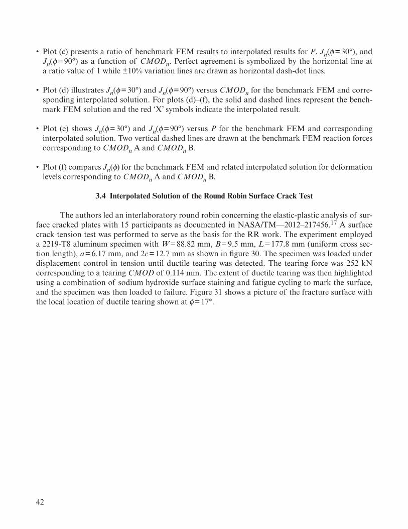
42

• Plot(c)presentsaratioofbenchmarkFEMresultstointerpolatedresultsforP,Jn(φ =30°),andJn(φ=90°)asa functionofCMODn.Perfectagreement is symbolizedby thehorizontal lineataratiovalueof1while±10%variationlinesaredrawnashorizontaldash-dotlines.

• Plot(d)illustratesJn(φ=30°)andJn(φ=90°)versusCMODnforthebenchmarkFEMandcorre-spondinginterpolatedsolution.Forplots(d)–(f),thesolidanddashedlinesrepresentthebench-markFEMsolutionandthered‘X’symbolsindicatetheinterpolatedresult.

• Plot (e) showsJn(φ=30°)andJn(φ=90°)versusP for thebenchmarkFEMandcorrespondinginterpolatedsolution.TwoverticaldashedlinesaredrawnatthebenchmarkFEMreactionforcescorrespondingtoCMODnAandCMODnB.

• Plot(f)comparesJn(φ)forthebenchmarkFEMandrelatedinterpolatedsolutionfordeformationlevelscorrespondingtoCMODnAandCMODnB.

3.4 Interpolated Solution of the Round Robin Surface Crack Test

Theauthorsledaninterlaboratoryroundrobinconcerningtheelastic-plasticanalysisofsur-facecrackedplateswith15participantsasdocumentedinNASA/TM—2012–217456.17AsurfacecracktensiontestwasperformedtoserveasthebasisfortheRRwork.Theexperimentemployeda2219-T8aluminumspecimenwithW=88.82mm,B=9.5mm,L=177.8mm(uniformcrosssec-tionlength),a=6.17mm,and2c=12.7mmasshowninfigure30.Thespecimenwasloadedunderdisplacementcontrol in tensionuntilductile tearingwasdetected.The tearing forcewas252kNcorrespondingtoatearingCMODof 0.114mm.Theextentofductiletearingwasthenhighlightedusingacombinationofsodiumhydroxidesurfacestainingandfatiguecyclingtomarkthesurface,andthespecimenwasthenloadedtofailure.Figure31showsapictureofthefracturesurfacewiththelocallocationofductiletearingshownatφ=17°.

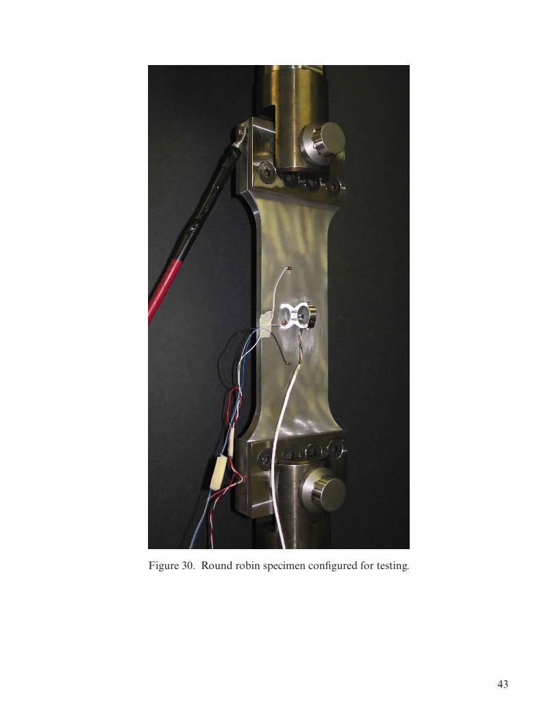
43

Figure 30. Round robin specimen configured for testing.

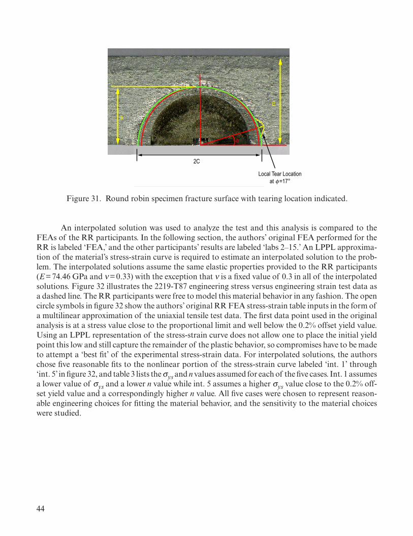
44

φ

B

a

2C

Local Tear Locationat =17°φ

Figure 31. Round robin specimen fracture surface with tearing location indicated.

An interpolated solution was used to analyze the test and this analysis is compared to the FEAs of the RR participants. In the following section, the authors’ original FEA performed for the RR is labeled ‘FEA,’ and the other participants’ results are labeled ‘labs 2–15.’ An LPPL approxima-tion of the material’s stress-strain curve is required to estimate an interpolated solution to the prob-lem. The interpolated solutions assume the same elastic properties provided to the RR participants (E = 74.46 GPa and ν = 0.33) with the exception that ν is a fixed value of 0.3 in all of the interpolated solutions. Figure 32 illustrates the 2219-T87 engineering stress versus engineering strain test data as a dashed line. The RR participants were free to model this material behavior in any fashion. The open circle symbols in figure 32 show the authors’ original RR FEA stress-strain table inputs in the form of a multilinear approximation of the uniaxial tensile test data. The first data point used in the original analysis is at a stress value close to the proportional limit and well below the 0.2% offset yield value. Using an LPPL representation of the stress-strain curve does not allow one to place the initial yield point this low and still capture the remainder of the plastic behavior, so compromises have to be made to attempt a ‘best fit’ of the experimental stress-strain data. For interpolated solutions, the authors chose five reasonable fits to the nonlinear portion of the stress-strain curve labeled ‘int. 1’ through ‘int. 5’ in figure 32, and table 3 lists the sys and n values assumed for each of the five cases. Int. 1 assumes a lower value of sys and a lower n value while int. 5 assumes a higher sys value close to the 0.2% off-set yield value and a correspondingly higher n value. All five cases were chosen to represent reason-able engineering choices for fitting the material behavior, and the sensitivity to the material choices were studied.

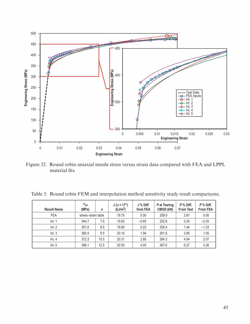
45

0 0.01 0.02 0.03 0.04 0.05 0.06 0.070

50

100

150

200

250

300

350

400

450

500

Engi

neer

ing

Stre

ss (M

Pa)

0 0.005 0.01 0.015 0.02 0.025 0.03300

350

400

450

Engineering Strain

Engineering Strain

Engi

neer

ing

Stre

ss (M

Pa)

Test DataFEA InputsInt. 1Int. 2Int. 3Int. 4Int. 5

Figure 32. Round robin uniaxial tensile stress versus strain data compared with FEA and LPPL material fits.

Table 3. Round robin FEM and interpolation method sensitivity study result comparisons.

Result Nameσys

(MPa) nJ (f = 17°)

(kJ/m2)J % Diff. from FEA

P at Tearing CMOD (kN)

P % Diff. From Test

P % Diff. From FEA

FEA stress–strain table 19.75 0.00 258.9 2.81 0.00Int. 1 344.7 7.5 19.63 –0.65 252.8 0.40 –2.35Int. 2 351.6 8.5 19.80 0.22 255.4 1.44 –1.33Int. 3 365.4 9.5 20.14 1.94 261.6 3.90 1.05Int. 4 372.3 10.5 20.31 2.80 264.3 4.94 2.07Int. 5 386.1 12.5 20.55 4.05 267.6 6.27 3.36

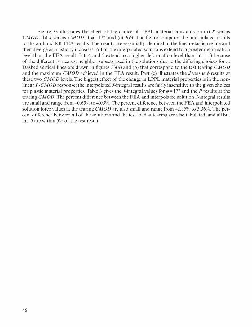
46

Figure 33 illustrates the effect of the choice of LPPL material constants on (a) P versus CMOD, (b) J versus CMOD at f = 17°, and (c) J(f). The figure compares the interpolated results to the authors’ RR FEA results. The results are essentially identical in the linear-elastic regime and then diverge as plasticity increases. All of the interpolated solutions extend to a greater deformation level than the FEA result. Int. 4 and 5 extend to a higher deformation level than int. 1–3 because of the different 16 nearest neighbor subsets used in the solutions due to the differing choices for n. Dashed vertical lines are drawn in figures 33(a) and (b) that correspond to the test tearing CMOD and the maximum CMOD achieved in the FEA result. Part (c) illustrates the J versus f results at these two CMOD levels. The biggest effect of the change in LPPL material properties is in the non-linear P-CMOD response; the interpolated J-integral results are fairly insensitive to the given choices for plastic material properties. Table 3 gives the J-integral values for f = 17° and the P results at the tearing CMOD. The percent difference between the FEA and interpolated solution J-integral results are small and range from –0.65% to 4.05%. The percent difference between the FEA and interpolated solution force values at the tearing CMOD are also small and range from –2.35% to 3.36%. The per-cent difference between all of the solutions and the test load at tearing are also tabulated, and all but int. 5 are within 5% of the test result.

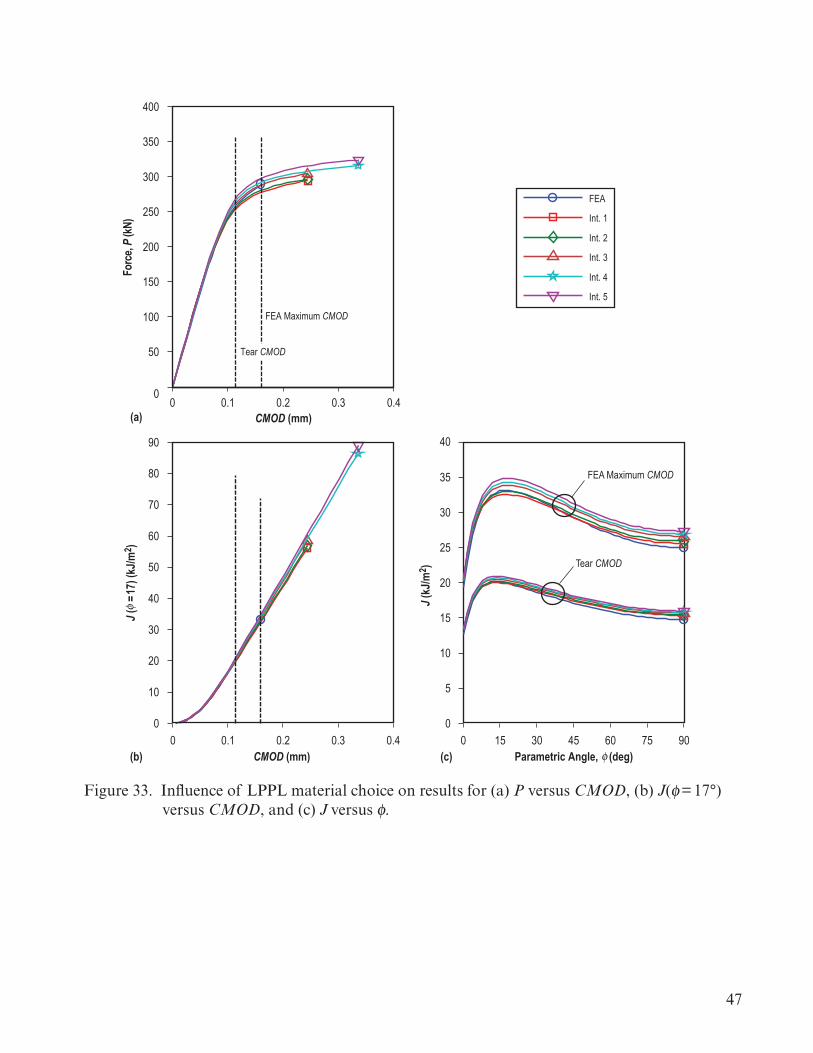
47

0 0.1 0.2 0.3 0.40

50

100

150

200

250

300

350

400

FEA Maximum CMOD

Tear CMOD

CMOD (mm)

Forc

e, P

(kN)

FEA

Int. 1

Int. 2

Int. 3

Int. 4

Int. 5

0 0.1 0.2 0.3 0.40

10

20

30

40

50

60

70

80

90

CMOD (mm)

(a)

(b) (c)0 15 30 45 60 75 90

0

5

10

15

20

25

30

35

40J (

kJ/m

2 )

J ( =

17) (

kJ/m

2 )

Parametric Angle, (deg)φ

φ

FEA Maximum CMOD

Tear CMOD

Figure 33. Influence of LPPL material choice on results for (a) P versus CMOD, (b) J(f = 17°) versus CMOD, and (c) J versus f.

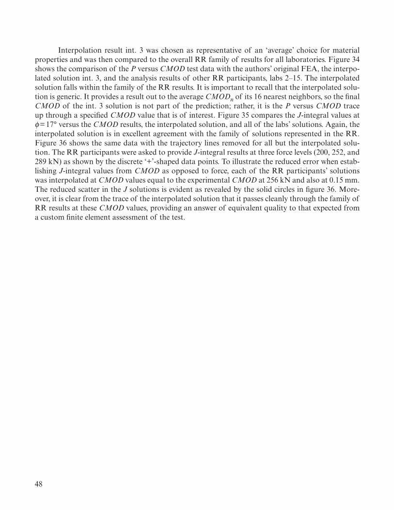
48

Interpolation result int. 3 was chosen as representative of an ‘average’ choice for material properties and was then compared to the overall RR family of results for all laboratories. Figure 34 shows the comparison of the P versus CMOD test data with the authors’ original FEA, the interpo-lated solution int. 3, and the analysis results of other RR participants, labs 2–15. The interpolated solution falls within the family of the RR results. It is important to recall that the interpolated solu-tion is generic. It provides a result out to the average CMODn of its 16 nearest neighbors, so the final CMOD of the int. 3 solution is not part of the prediction; rather, it is the P versus CMOD trace up through a specified CMOD value that is of interest. Figure 35 compares the J-integral values at f = 17° versus the CMOD results, the interpolated solution, and all of the labs’ solutions. Again, the interpolated solution is in excellent agreement with the family of solutions represented in the RR. Figure 36 shows the same data with the trajectory lines removed for all but the interpolated solu-tion. The RR participants were asked to provide J-integral results at three force levels (200, 252, and 289 kN) as shown by the discrete ‘+’-shaped data points. To illustrate the reduced error when estab-lishing J-integral values from CMOD as opposed to force, each of the RR participants’ solutions was interpolated at CMOD values equal to the experimental CMOD at 256 kN and also at 0.15 mm. The reduced scatter in the J solutions is evident as revealed by the solid circles in figure 36. More-over, it is clear from the trace of the interpolated solution that it passes cleanly through the family of RR results at these CMOD values, providing an answer of equivalent quality to that expected from a custom finite element assessment of the test.

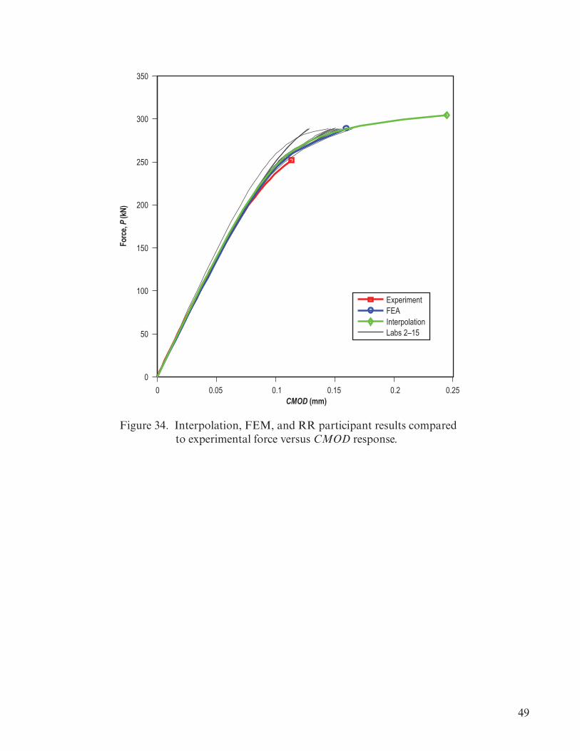
49

0 0.05 0.1 0.15 0.2 0.250

50

100

150

200

250

300

350

CMOD (mm)

Forc

e, P

(kN)

ExperimentFEAInterpolationLabs 2–15

Figure 34. Interpolation, FEM, and RR participant results compared to experimental force versus CMOD response.

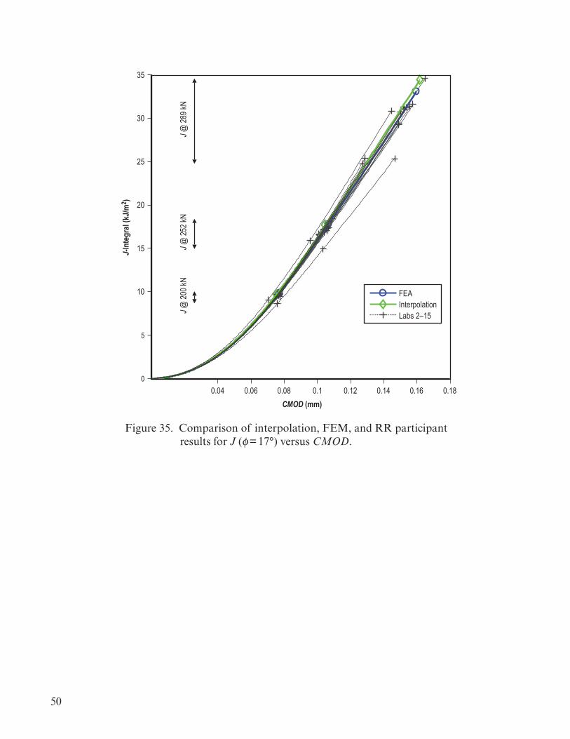
50

0.04 0.06 0.08 0.1 0.12 0.14 0.16 0.180

5

10

15

20

25

30

35

J @ 28

9 kN

J @ 25

2 kN

J @ 20

0 kN

CMOD (mm)

J-In

tegr

al (k

J/m2 )

FEAInterpolationLabs 2–15

Figure 35. Comparison of interpolation, FEM, and RR participant results for J (f = 17°) versus CMOD.

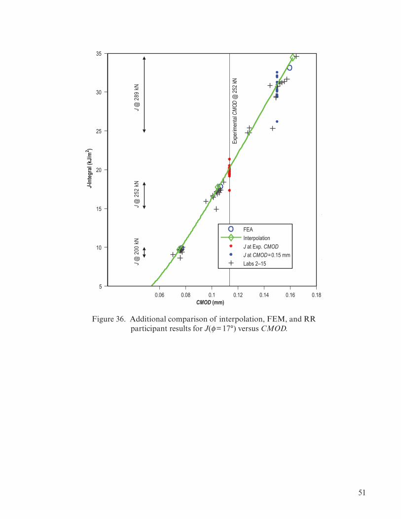
51

0.06 0.08 0.1 0.12 0.14 0.16 0.185

10

15

20

25

30

35

Expe

rimen

tal C

MOD

@ 25

2 kN

J @ 2

89 k

NJ @

252

kN

J @ 2

00 k

N

CMOD (mm)

J-In

tegr

al (k

J/m2 )

FEAInterpolationJ at Exp. CMODJ at CMOD=0.15 mmLabs 2–15

Figure 36. Additional comparison of interpolation, FEM, and RR participant results for J(f = 17°) versus CMOD.

52

4. CONCLUSIONS

This set of elastic-plastic surface crack solutions and the interpolation methodologies devel-oped to sew them together into a complete, functional space represents a significant bridge for the practicing engineer toward commonplace assessment of surface cracks by the J-integral. This is par-ticularly true for the case of experimental evaluation of surface crack performance. The evaluation of fracture toughness in the elastic-plastic regime continues to lag significantly behind linear-elastic methods in implementation experimentally, even for common 2D geometries such as the C(T) speci-men, despite the advantages in flexibility and breadth of information elastic-plastic methods reveal. Surface crack toughness testing can provide the most direct measure of material performance in structurally representative configurations; yet, the detailed working knowledge of finite element mod-eling required to properly assess a surface crack test in the elastic-plastic regime (as most are) has kept surface crack toughness testing reserved mainly as a domain for the specialist. The costs in modeling time and software infrastructure are largely prohibitive for most experimental labs. The interpolation methodology described herein and solution space provided in the appendices represent a new evolu-tional step in tools for the analyst and experimentalist alike. Significant effort has been expended to ensure the reliability of this new tool. The authors have verified the solutions and the interpolation method through several techniques. The linear-elastic J-integral solutions were shown to be very similar to the Newman-Raju solutions. Domain conver-gence for the elastic-plastic J-integral values at the final load step was demonstrated for the complete set of solutions at all crack front locations. Twenty-five benchmark FEMs were created purposefully exploiting gaps in the geometry and material solution matrices to test the effectiveness of the interpo-lation method. The interpolated solutions were able to predict the benchmark J-integral and reaction force solutions for a given CMOD value to within a few percent. The interpolation method was also used to estimate a solution for an interlaboratory round robin problem, and the interpolated solution had excellent agreement with the multiple laboratory results. The results of these studies indicate that the authors’ surface crack solution set and interpolation method are sufficiently accurate to provide easily obtained and useful solutions for the J-integral and P-CMOD response.

There remain a number of refinements and extensions to this work that would be equally valuable. The most obvious extension is to develop a similar solution space for surface cracks in flat plates subjected to a bending stress boundary condition. This is feasible with much of the same framework used to create the tension case. Within the existing tension space there are opportunities to fill gaps in the geometric or material variables to improve interpolation errors or to implement more sophisticated interpolation schemes. This may be a warranted investigation prior to developing the bending solutions. The solution set provides an excellent opportunity to investigate general surface crack behavior such as refining surface crack deformation limits in LEFM and EPFM, developing a robust predictor of surface crack tearing location in f, or extrapolating solutions to higher deforma-tion levels. Despite the many possibilities, the most hopeful outcome for the authors is adoption in the experimental community. Perhaps these solutions will eventually provide an impact similar to the equations of Newman and Raju.

53

APPENDIX A—WIDTH EFFECTS SUBSTUDY

A substudy was conducted to investigate the effects of increasing W/2c on the J-integral solu-tions and the force versus CMOD response. The same model used in the normalization case study was utilized here with W/2c = 5, L/W = 2, a/B = 0.6, a/c = 0.6, n = 6, sys = 1, ν = 0.3, and E/sys = 300. Two additional FEMs were created and analyzed with W/2c = 10 and 20 with all other geometric propor-tions and properties the same. In addition, interpolated solutions were estimated for all three plate geometries. Figure 37 illustrates the normalized far-field stress, sn, versus CMODn for all the FEMs and interpolated solutions. All of the sn versus CMODn interpolated solutions are identical and match the W/2c = 5 FEM result, and all of the responses are essentially the same in the linear-elastic region. The wider FEM plate results require a slightly higher far-field stress to reach a given CMODn value in the nonlinear region. Figure 38 shows the figure 37 results with the stress axis converted to applied force, P. As expected, the interpolated result and the W/2c = 5 FEM result match exactly. The interpolated solutions of the wider plate results are a reasonable match in the linear regime, but the interpolated results slightly underpredict the force for a given CMODn in the nonlinear region. Matching the P versus CMODn response is not required to interpolate to a J-integral solution, but is important for a comparison to P versus CMOD experimental results. Figure 39 illustrates that the Jn(f = 90°) versus CMODn results are almost identical for the FEA and interpolated solutions show-ing that the J-integral as a function of CMOD is essentially invariant to increasing plate width. The maximum CMODn for the W/2c = 20 FEM is shown as a vertical dashed line in figure 39, and figure 40 shows Jn versus f results at this CMODn level for all the FEA and interpolated solutions. Again, the Jn versus f results are demonstrated to be insensitive to plate width for a given CMODn level, and the interpolated solutions are an excellent match to the FEA solutions.

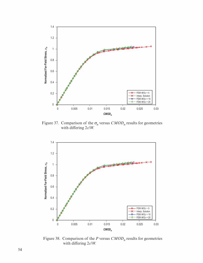
54

0 0.005 0.01 0.015 0.02 0.025 0.030

0.2

0.4

0.6

0.8

1

1.2

1.4

FEM W/2c = 5Interp. SolutionFEM W/2c = 10FEM W/2c = 20

CMODn

σ nNo

rmali

zed

Far-F

ield

Stre

ss,

Figure 37. Comparison of the sn versus CMODn results for geometries with differing 2c/W.

0 0.005 0.01 0.015 0.02 0.025 0.030

0.2

0.4

0.6

0.8

1

1.2

1.4


CMODn

σ nNo

rmali

zed

Far-F

ield

Stre

ss,

Figure 38. Comparison of the P versus CMODn results for geometries with differing 2c/W.

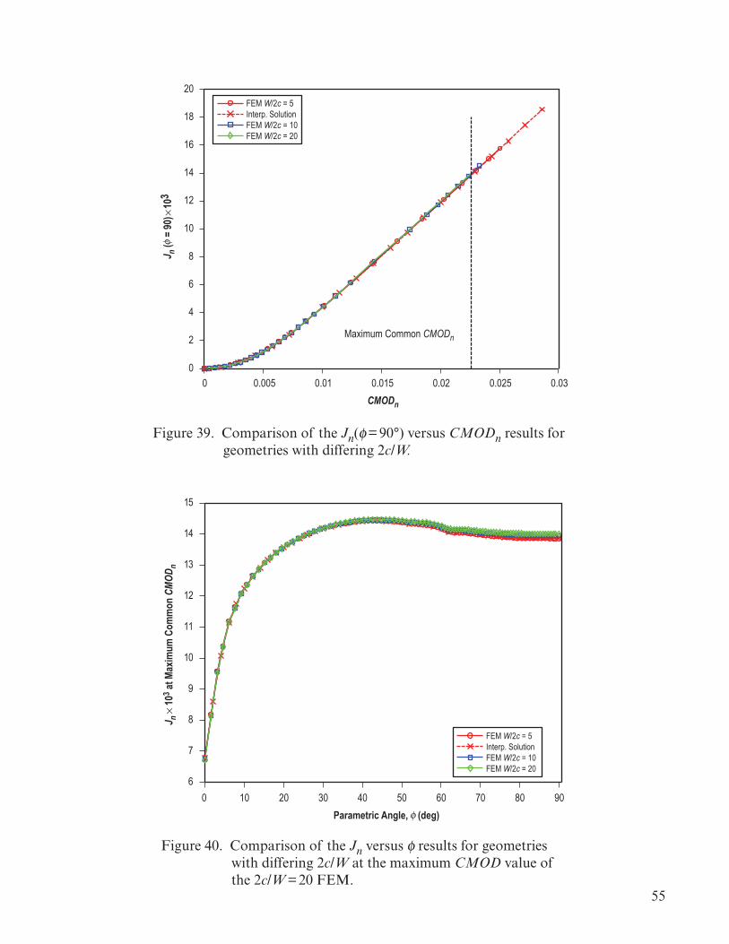
55

0 0.005 0.01 0.015 0.02 0.025 0.030

2

4

6

8

10

12

14

16

18

20

CMODn


φJ n (

= 90

)×10

3


Figure 39. Comparison of the Jn(f = 90°) versus CMODn results for geometries with differing 2c/W.

0 10 20 30 40 50 60 70 80 906

7

8

9

10

11

12

13

14

15

J n ×

103 a

t Max

imum

Com

mon

CMO

D n


φParametric Angle, (deg)

Figure 40. Comparison of the Jn versus f results for geometries with differing 2c/W at the maximum CMOD value of the 2c/W = 20 FEM.

56

APPENDIX B—COLLECTION OF BENCHMARK MODELS COMPARISON PLOTS

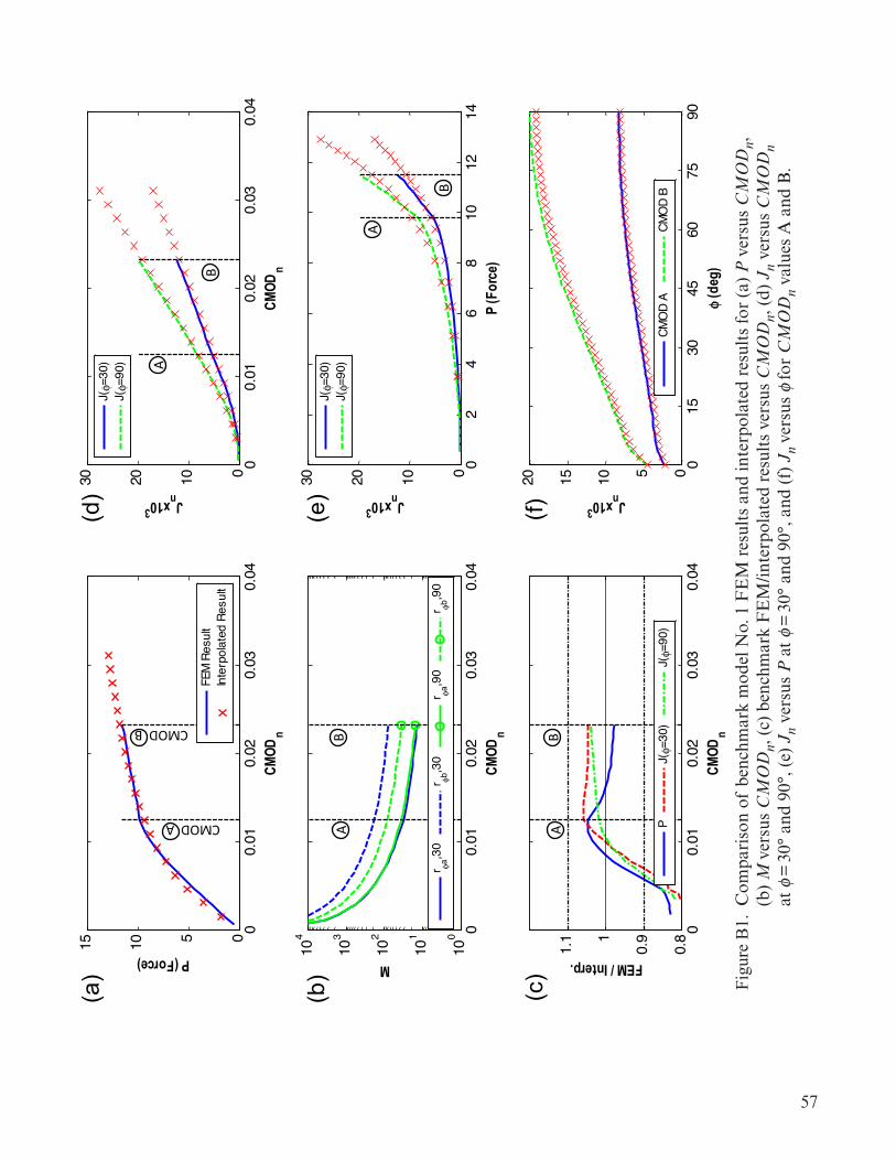
57

00.

010.

020.

030.

04051015

CMOD

n

P (Force)

FEM

Res

ult

Inte

rpol

ated

Res

ult

00.

010.

020.

030.

040102030

CMOD

n

Jnx103

J(φ=

30)

J(φ=

90)

00.

010.

020.

030.

0410

0

101

102

103

104

CMOD

n

M

r φa,3

0r φb

,30

r φa,9

0r φb

,90

02

46

810

1214

0102030

P (F

orce

)

Jnx103

J(φ=

30)

J(φ=

90)

00.

010.

020.

030.

040.

8

0.91

1.1

CMOD

n

FEM / Interp.

PJ(φ=

30)

J(φ=

90)

015

3045

6075

9005101520

φ (d

eg)

Jnx103

CMO

D A

CMO

D B

CMOD A

CMOD B

AB

AB

A

B

A

B

Fig. B1

(a)

(b)

(c)

(d)

(e)

(f)

Figu

re B

1. C

ompa

riso

n of

ben

chm

ark

mod

el N

o. 1

FE

M r

esul

ts a

nd in

terp

olat

ed r

esul

ts fo

r (a

) P

ver

sus

CM

OD

n,

(b)

M v

ersu

s C

MO

Dn,

(c)

ben

chm

ark

FE

M/in

terp

olat

ed r

esul

ts v

ersu

s C

MO

Dn,

(d)

Jn

vers

us C

MO

Dn

at

f =

30°

and

90°

, (e)

Jn

vers

us P

at

f = 3

0° a

nd 9

0°, a

nd (

f) J

n ve

rsus

f fo

r C

MO

Dn

valu

es A

and

B.

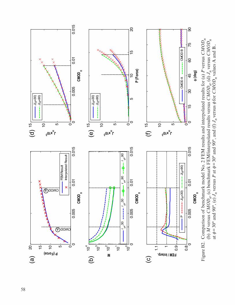
58

00.

005

0.01

0.01

505101520

CMOD

n

P (Force)

FEM

Res

ult

Inte

rpol

ated

Res

ult

00.

005

0.01

0.01

5051015

CMOD

n

Jnx103

J(φ=

30)

J(φ=

90)

00.

005

0.01

0.01

510

0

101

102

103

104

CMOD

n

M

r φa,3

0r φb

,30

r φa,9

0r φb

,90

05

1015

20051015

P (F

orce

)

Jnx103

J(φ=

30)

J(φ=

90)

00.

005

0.01

0.01

50.

8

0.91

1.1

CMOD

n

FEM / Interp.

PJ(φ=

30)

J(φ=

90)

015

3045

6075

90051015

φ (d

eg)

Jnx103

CMO

D A

CMO

D B

CMOD A

CMOD B

Fig. B2

(a)

(b)

(c)

(d)

(e)

(f)

Figu

re B

2. C

ompa

riso

n of

ben

chm

ark

mod

el N

o. 2

FE

M r

esul

ts a

nd in

terp

olat

ed r

esul

ts fo

r (a

) P

ver

sus

CM

OD

n (b

) M

ver

sus

CM

OD

n, (

c) b

ench

mar

k F

EM

/inte

rpol

ated

res

ults

ver

sus

CM

OD

n, (

d) J

n ve

rsus

CM

OD

n

at f

= 3

0° a

nd 9

0°, (

e) J

n ve

rsus

P a

t f =

30°

and

90°

, and

(f)

Jn

vers

us f

for

CM

OD

n va

lues

A a

nd B

..

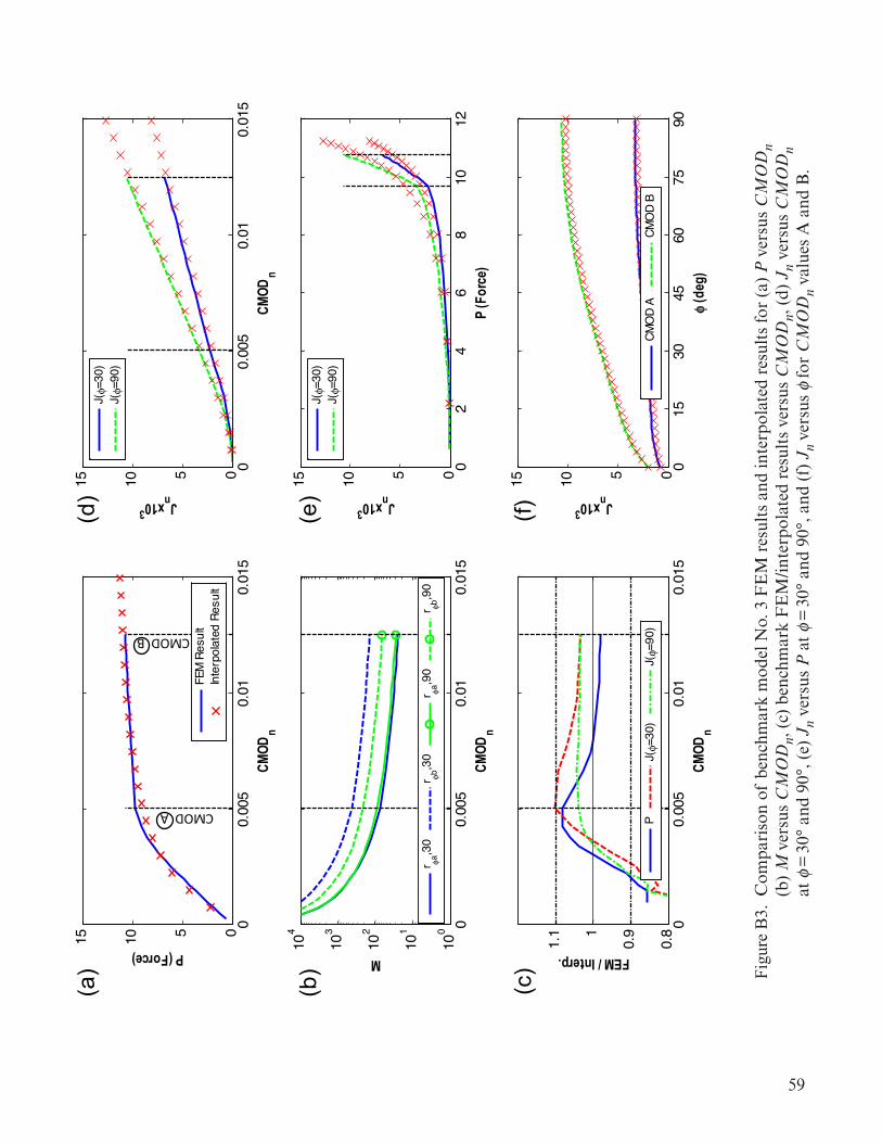
59

00.

005

0.01

0.01

5051015

CMOD

n

P (Force)

FEM

Res

ult

Inte

rpol

ated

Res

ult

00.

005

0.01

0.01

5051015

CMOD

n

Jnx103

J(φ=

30)

J(φ=

90)

00.

005

0.01

0.01

510

0

101

102

103

104

CMOD

n

M

r φa,3

0r φb

,30

r φa,9

0r φb

,90

02

46

810

12051015

P (F

orce

)

Jnx103

J(φ=

30)

J(φ=

90)

00.

005

0.01

0.01

50.

8

0.91

1.1

CMOD

n

FEM / Interp.

PJ(φ=

30)

J(φ=

90)

015

3045

6075

90051015

φ (d

eg)

Jnx103

CMO

D A

CMO

D B

CMOD A

CMOD B

Fig. B3

(a)

(b)

(c)

(d)

(e)

(f)

Figu

re B

3. C

ompa

riso

n of

ben

chm

ark

mod

el N

o. 3

FE

M r

esul

ts a

nd in

terp

olat

ed r

esul

ts fo

r (a

) P

ver

sus

CM

OD

n (b

) M

ver

sus

CM

OD

n, (

c) b

ench

mar

k F

EM

/inte

rpol

ated

res

ults

ver

sus

CM

OD

n, (

d) J

n ve

rsus

CM

OD

n

at f

= 3

0° a

nd 9

0°, (

e) J

n ve

rsus

P a

t f =

30°

and

90°

, and

(f)

Jn

vers

us f

for

CM

OD

n va

lues

A a

nd B

.

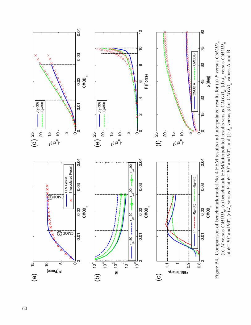
60

00.

010.

020.

030.

04051015

CMOD

n

P (Force)

FEM

Res

ult

Inte

rpol

ated

Res

ult

00.

010.

020.

030.

040510152025

CMOD

n

Jnx103

J(φ=

30)

J(φ=

90)

00.

010.

020.

030.

0410

0

101

102

103

104

CMOD

n

M

r φa,3

0r φb

,30

r φa,9

0r φb

,90

02

46

810

120510152025

P (F

orce

)

Jnx103

J(φ=

30)

J(φ=

90)

00.

010.

020.

030.

040.

8

0.91

1.1

CMOD

n

FEM / Interp.

PJ(φ=

30)

J(φ=

90)

015

3045

6075

900510152025

φ (d

eg)

Jnx103

CMO

D A

CMO

D B

CMOD A

CMOD B

Fig. B4

(a)

(b)

(c)

(d)

(e)

(f)

Figu

re B

4. C

ompa

riso

n of

ben

chm

ark

mod

el N

o. 4

FE

M r

esul

ts a

nd in

terp

olat

ed r

esul

ts fo

r (a

) P

ver

sus

CM

OD

n

(b)

M v

ersu

s C

MO

Dn,

(c)

ben

chm

ark

FE

M/in

terp

olat

ed r

esul

ts v

ersu

s C

MO

Dn,

(d)

Jn

vers

us C

MO

Dn

at

f =

30°

and

90°

, (e)

Jn

vers

us P

at

f = 3

0° a

nd 9

0°, a

nd (

f) J

n ve

rsus

f fo

r C

MO

Dn

valu

es A

and

B.

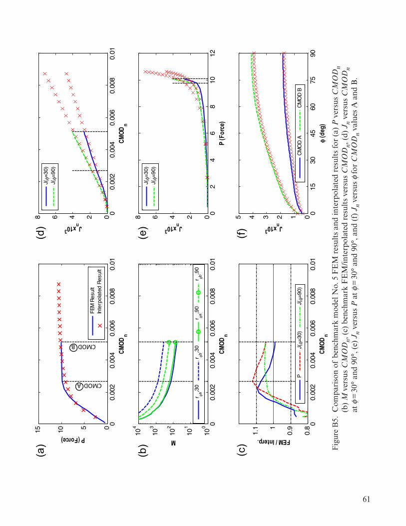
61

Figu

re B

4. C

ompa

riso

n of

ben

chm

ark

mod

el N

o. 4

FE

M r

esul

ts a

nd in

terp

olat

ed r

esul

ts fo

r (a

) P

ver

sus

CM

OD

n

(b)

M v

ersu

s C

MO

Dn,

(c)

ben

chm

ark

FE

M/in

terp

olat

ed r

esul

ts v

ersu

s C

MO

Dn,

(d)

Jn

vers

us C

MO

Dn

at

f =

30°

and

90°

, (e)

Jn

vers

us P

at

f = 3

0° a

nd 9

0°, a

nd (

f) J

n ve

rsus

f fo

r C

MO

Dn

valu

es A

and

B.

00.

002

0.00

40.

006

0.00

80.

01051015

CMOD

n

P (Force)

FEM

Res

ult

Inte

rpol

ated

Res

ult

00.

002

0.00

40.

006

0.00

80.

0102468

CMOD

n

Jnx103

J(φ=

30)

J(φ=

90)

00.

002

0.00

40.

006

0.00

80.

0110

0

101

102

103

104

CMOD

n

M

r φa,3

0r φb

,30

r φa,9

0r φb

,90

02

46

810

1202468

P (F

orce

)

Jnx103

J(φ=

30)

J(φ=

90)

00.

002

0.00

40.

006

0.00

80.

010.

8

0.91

1.1

CMOD

n

FEM / Interp.

PJ(φ=

30)

J(φ=

90)

015

3045

6075

90012345

φ (d

eg)

Jnx103

CMO

D A

CMO

D B

CMOD A

CMOD B

Fig. B5

(a)

(b)

(c)

(d)

(e)

(f)

Figu

re B

5. C

ompa

riso

n of

ben

chm

ark

mod

el N

o. 5

FE

M r

esul

ts a

nd in

terp

olat

ed r

esul

ts fo

r (a

) P

ver

sus

CM

OD

n (b

) M

ver

sus

CM

OD

n, (

c) b

ench

mar

k F

EM

/inte

rpol

ated

res

ults

ver

sus

CM

OD

n, (

d) J

n ve

rsus

CM

OD

n

at f

= 3

0° a

nd 9

0°, (

e) J

n ve

rsus

P a

t f =

30°

and

90°

, and

(f)

Jn

vers

us f

for

CM

OD

n va

lues

A a

nd B

.

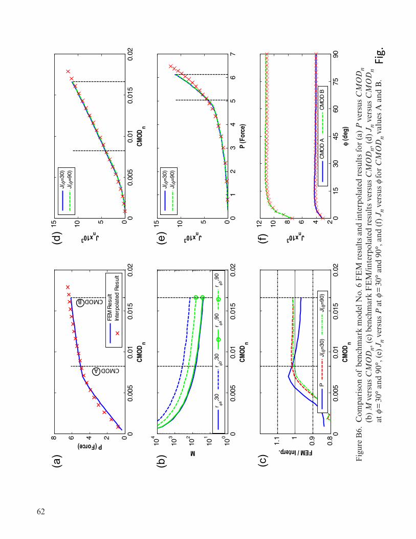
62

00.

005

0.01

0.01

50.

0202468

CMOD

n

P (Force)

FEM

Res

ult

Inte

rpol

ated

Res

ult

00.

005

0.01

0.01

50.

02051015

CMOD

n

Jnx103

J(φ=

30)

J(φ=

90)

00.

005

0.01

0.01

50.

0210

0

101

102

103

104

CMOD

n

M

r φa,3

0r φb

,30

r φa,9

0r φb

,90

01

23

45

67

051015

P (F

orce

)

Jnx103

J(φ=

30)

J(φ=

90)

00.

005

0.01

0.01

50.

020.

8

0.91

1.1

CMOD

n

FEM / Interp.

PJ(φ=

30)

J(φ=

90)

015

3045

6075

9024681012

φ (d

eg)

Jnx103

CMO

D A

CMO

D B

CMOD A

CMOD B

Fig. B6

(a)

(b)

(c)

(d)

(e)

(f)

Figu

re B

6. C

ompa

riso

n of

ben

chm

ark

mod

el N

o. 6

FE

M r

esul

ts a

nd in

terp

olat

ed r

esul

ts fo

r (a

) P

ver

sus

CM

OD

n

(b)

M v

ersu

s C

MO

Dn,

(c)

ben

chm

ark

FE

M/in

terp

olat

ed r

esul

ts v

ersu

s C

MO

Dn,

(d)

Jn

vers

us C

MO

Dn

at

f =

30°

and

90°

, (e)

Jn

vers

us P

at

f = 3

0° a

nd 9

0°, a

nd (

f) J

n ve

rsus

f fo

r C

MO

Dn

valu

es A

and

B.

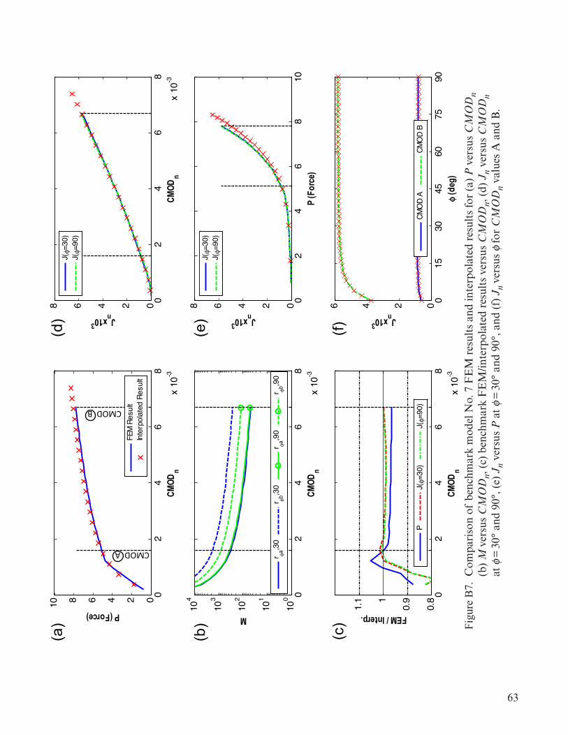
63

Figu

re B

6. C

ompa

riso

n of

ben

chm

ark

mod

el N

o. 6

FE

M r

esul

ts a

nd in

terp

olat

ed r

esul

ts fo

r (a

) P

ver

sus

CM

OD

n

(b)

M v

ersu

s C

MO

Dn,

(c)

ben

chm

ark

FE

M/in

terp

olat

ed r

esul

ts v

ersu

s C

MO

Dn,

(d)

Jn

vers

us C

MO

Dn

at

f =

30°

and

90°

, (e)

Jn

vers

us P

at

f = 3

0° a

nd 9

0°, a

nd (

f) J

n ve

rsus

f fo

r C

MO

Dn

valu

es A

and

B.

02

46

8x

10-3

0246810

CMOD

n

P (Force)

FEM

Res

ult

Inte

rpol

ated

Res

ult

02

46

8x

10-3

02468

CMOD

n

Jnx103

J(φ=

30)

J(φ=

90)

02

46

8x

10-3

100

101

102

103

104

CMOD

n

M

r φa,3

0r φb

,30

r φa,9

0r φb

,90

02

46

810

02468

P (F

orce

)

Jnx103

J(φ=

30)

J(φ=

90)

02

46

8x

10-3

0.8

0.91

1.1

CMOD

n

FEM / Interp.

PJ(φ=

30)

J(φ=

90)

015

3045

6075

900246

φ (d

eg)

Jnx103

CMO

D A

CMO

D B

CMOD A

CMOD B

Fig. B7

(a)

(b)

(c)

(d)

(e)

(f)

Figu

re B

7. C

ompa

riso

n of

ben

chm

ark

mod

el N

o. 7

FE

M r

esul

ts a

nd in

terp

olat

ed r

esul

ts fo

r (a

) P

ver

sus

CM

OD

n

(b)

M v

ersu

s C

MO

Dn,

(c)

ben

chm

ark

FE

M/in

terp

olat

ed r

esul

ts v

ersu

s C

MO

Dn,

(d)

Jn

vers

us C

MO

Dn

at

f =

30°

and

90°

, (e)

Jn

vers

us P

at

f = 3

0° a

nd 9

0°, a

nd (

f) J

n ve

rsus

f fo

r C

MO

Dn

valu

es A

and

B.

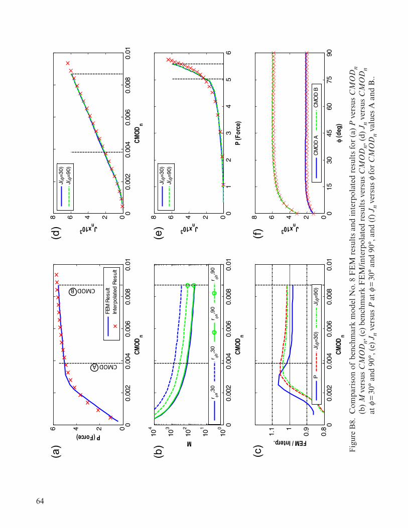
64

00.

002

0.00

40.

006

0.00

80.

010246

CMOD

n

P (Force)

FEM

Res

ult

Inte

rpol

ated

Res

ult

00.

002

0.00

40.

006

0.00

80.

0102468

CMOD

n

Jnx103

J(φ=

30)

J(φ=

90)

00.

002

0.00

40.

006

0.00

80.

0110

0

101

102

103

104

CMOD

n

M

r φa,3

0r φb

,30

r φa,9

0r φb

,90

01

23

45

602468

P (F

orce

)

Jnx103

J(φ=

30)

J(φ=

90)

00.

002

0.00

40.

006

0.00

80.

010.

8

0.91

1.1

CMOD

n

FEM / Interp.

PJ(φ=

30)

J(φ=

90)

015

3045

6075

9002468

φ (d

eg)

Jnx103

CMO

D A

CMO

D B

CMOD A

CMOD B

Fig. B8

(a)

(b)

(c)

(d)

(e)

(f)

Figu

re B

8. C

ompa

riso

n of

ben

chm

ark

mod

el N

o. 8

FE

M r

esul

ts a

nd in

terp

olat

ed r

esul

ts fo

r (a

) P

ver

sus

CM

OD

n

(b)

M v

ersu

s C

MO

Dn,

(c)

ben

chm

ark

FE

M/in

terp

olat

ed r

esul

ts v

ersu

s C

MO

Dn,

(d)

Jn

vers

us C

MO

Dn

at

f =

30°

and

90°

, (e)

Jn

vers

us P

at

f = 3

0° a

nd 9

0°, a

nd (

f) J

n ve

rsus

f fo

r C

MO

Dn

valu

es A

and

B..

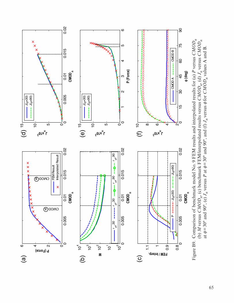
65

Figu

re B

8. C

ompa

riso

n of

ben

chm

ark

mod

el N

o. 8

FE

M r

esul

ts a

nd in

terp

olat

ed r

esul

ts fo

r (a

) P

ver

sus

CM

OD

n

(b)

M v

ersu

s C

MO

Dn,

(c)

ben

chm

ark

FE

M/in

terp

olat

ed r

esul

ts v

ersu

s C

MO

Dn,

(d)

Jn

vers

us C

MO

Dn

at

f =

30°

and

90°

, (e)

Jn

vers

us P

at

f = 3

0° a

nd 9

0°, a

nd (

f) J

n ve

rsus

f fo

r C

MO

Dn

valu

es A

and

B..

00.

005

0.01

0.01

50.

020246

CMOD

n

P (Force)

FEM

Res

ult

Inte

rpol

ated

Res

ult

00.

005

0.01

0.01

50.

02051015

CMOD

n

Jnx103

J(φ=

30)

J(φ=

90)

00.

005

0.01

0.01

50.

0210

0

101

102

103

104

CMOD

n

M

r φa,3

0r φb

,30

r φa,9

0r φb

,90

01

23

45

6051015

P (F

orce

)

Jnx103

J(φ=

30)

J(φ=

90)

00.

005

0.01

0.01

50.

020.

8

0.91

1.1

CMOD

n

FEM / Interp.

PJ(φ=

30)

J(φ=

90)

015

3045

6075

90246810

φ (d

eg)

Jnx103

CMO

D A

CMO

D B

CMOD A

CMOD B

Fig. B9

(a)

(b)

(c)

(d)

(e)

(f)

Figu

re B

9. C

ompa

riso

n of

ben

chm

ark

mod

el N

o. 9

FE

M r

esul

ts a

nd in

terp

olat

ed r

esul

ts fo

r (a

) P

ver

sus

CM

OD

n (b

) M

ver

sus

CM

OD

n, (

c) b

ench

mar

k F

EM

/inte

rpol

ated

res

ults

ver

sus

CM

OD

n, (

d) J

n ve

rsus

CM

OD

n

at f

= 3

0° a

nd 9

0°, (

e) J

n ve

rsus

P a

t f =

30°

and

90°

, and

(f)

Jn

vers

us f

for

CM

OD

n va

lues

A a

nd B

.

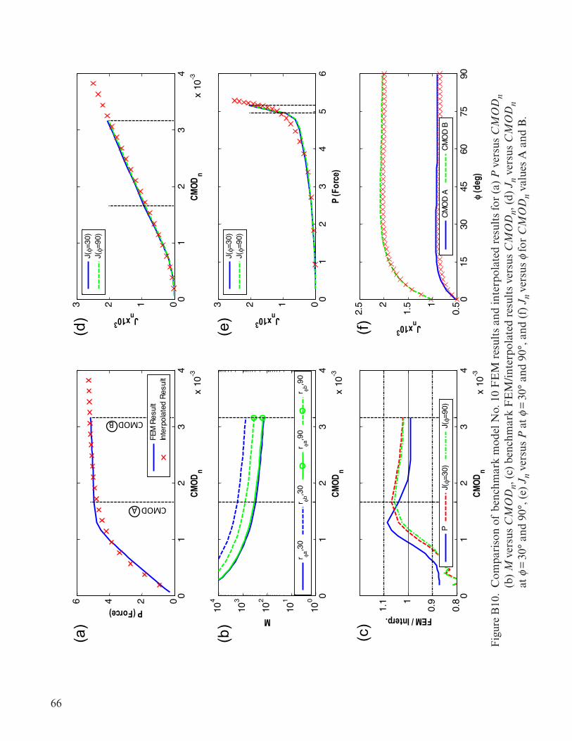
66

01

23

4x

10-3

0246

CMOD

n

P (Force)

FEM

Res

ult

Inte

rpol

ated

Res

ult

01

23

4x

10-3

0123

CMOD

n

Jnx103

J(φ=

30)

J(φ=

90)

01

23

4x

10-3

100

101

102

103

104

CMOD

n

M

r φa,3

0r φb

,30

r φa,9

0r φb

,90

01

23

45

60123

P (F

orce

)

Jnx103

J(φ=

30)

J(φ=

90)

01

23

4x

10-3

0.8

0.91

1.1

CMOD

n

FEM / Interp.

PJ(φ=

30)

J(φ=

90)

015

3045

6075

900.

51

1.52

2.5

φ (d

eg)

Jnx103

CMO

D A

CMO

D B

CMOD A

CMOD B

Fig. B10

(a)

(b)

(c)

(d)

(e)

(f)

Figu

re B

10.

Com

pari

son

of b

ench

mar

k m

odel

No.

10

FE

M r

esul

ts a

nd in

terp

olat

ed r

esul

ts fo

r (a

) P

ver

sus

CM

OD

n (b

) M

ver

sus

CM

OD

n, (

c) b

ench

mar

k F

EM

/inte

rpol

ated

res

ults

ver

sus

CM

OD

n, (

d) J

n ve

rsus

CM

OD

n

at f

= 3

0° a

nd 9

0°, (

e) J

n ve

rsus

P a

t f =

30°

and

90°

, and

(f)

Jn

vers

us f

for

CM

OD

n va

lues

A a

nd B

.

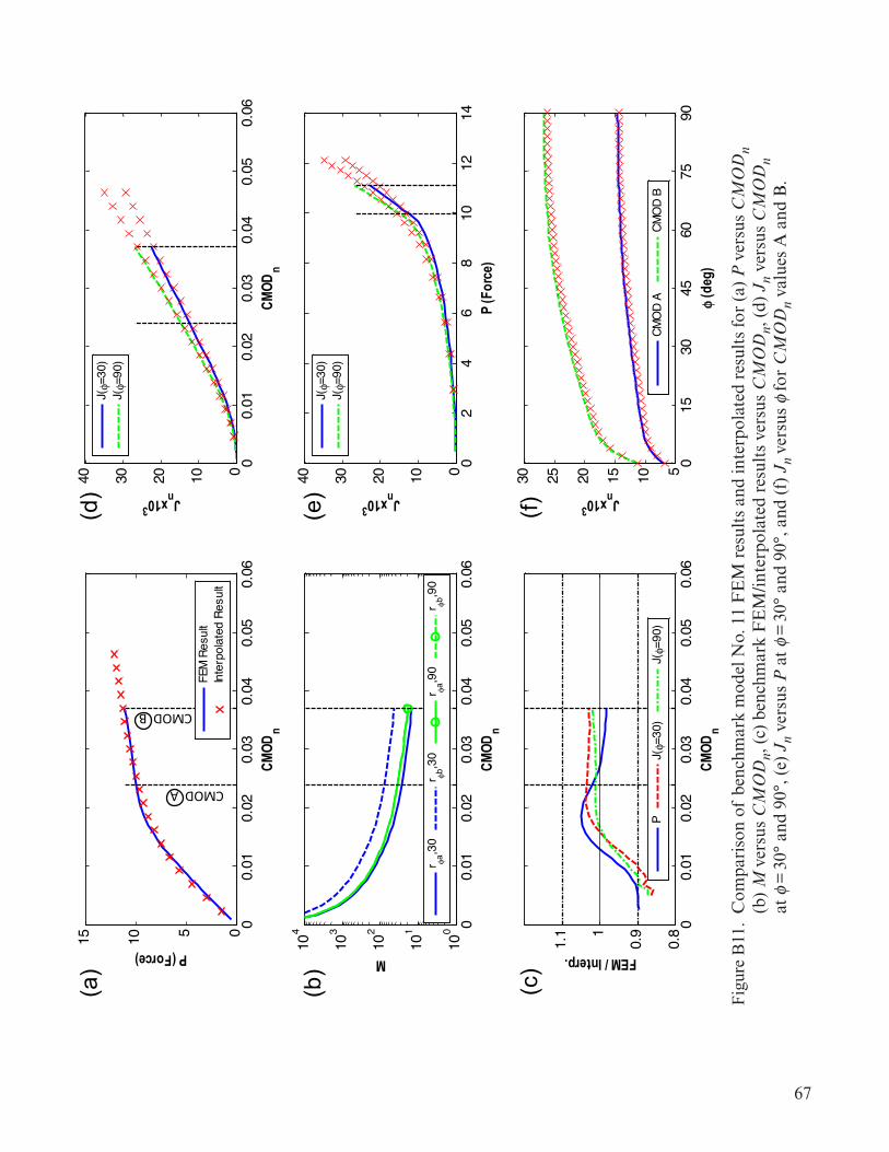
67

Figu

re B

10.

Com

pari

son

of b

ench

mar

k m

odel

No.

10

FE

M r

esul

ts a

nd in

terp

olat

ed r

esul

ts fo

r (a

) P

ver

sus

CM

OD

n (b

) M

ver

sus

CM

OD

n, (

c) b

ench

mar

k F

EM

/inte

rpol

ated

res

ults

ver

sus

CM

OD

n, (

d) J

n ve

rsus

CM

OD

n

at f

= 3

0° a

nd 9

0°, (

e) J

n ve

rsus

P a

t f =

30°

and

90°

, and

(f)

Jn

vers

us f

for

CM

OD

n va

lues

A a

nd B

.

00.

010.

020.

030.

040.

050.

06051015

CMOD

n

P (Force)

FEM

Res

ult

Inte

rpol

ated

Res

ult

00.

010.

020.

030.

040.

050.

06010203040

CMOD

n

Jnx103

J(φ=

30)

J(φ=

90)

00.

010.

020.

030.

040.

050.

0610

0

101

102

103

104

CMOD

n

M

r φa,3

0r φb

,30

r φa,9

0r φb

,90

02

46

810

1214

010203040

P (F

orce

)

Jnx103

J(φ=

30)

J(φ=

90)

00.

010.

020.

030.

040.

050.

060.

8

0.91

1.1

CMOD

n

FEM / Interp.

PJ(φ=

30)

J(φ=

90)

015

3045

6075

9051015202530

φ (d

eg)

Jnx103

CMO

D A

CMO

D B

CMOD A

CMOD B

Fig. B11

(a)

(b)

(c)

(d)

(e)

(f)

Figu

re B

11.

Com

pari

son

of b

ench

mar

k m

odel

No.

11

FE

M r

esul

ts a

nd in

terp

olat

ed r

esul

ts fo

r (a

) P

ver

sus

CM

OD

n (b

) M

ver

sus

CM

OD

n, (

c) b

ench

mar

k F

EM

/inte

rpol

ated

res

ults

ver

sus

CM

OD

n, (

d) J

n ve

rsus

CM

OD

n

at f

= 3

0° a

nd 9

0°, (

e) J

n ve

rsus

P a

t f =

30°

and

90°

, and

(f)

Jn

vers

us f

for

CM

OD

n va

lues

A a

nd B

.

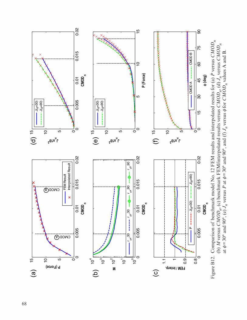
68

00.

005

0.01

0.01

50.

02051015

CMOD

n

P (Force)

FEM

Res

ult

Inte

rpol

ated

Res

ult

00.

005

0.01

0.01

50.

02051015

CMOD

n

Jnx103

J(φ=

30)

J(φ=

90)

00.

005

0.01

0.01

50.

0210

0

101

102

103

104

CMOD

n

M

r φa,3

0r φb

,30

r φa,9

0r φb

,90

05

1015

051015

P (F

orce

)

Jnx103

J(φ=

30)

J(φ=

90)

00.

005

0.01

0.01

50.

020.

8

0.91

1.1

CMOD

n

FEM / Interp.

PJ(φ=

30)

J(φ=

90)

015

3045

6075

90051015

φ (d

eg)

Jnx103

CMO

D A

CMO

D B

CMOD A

CMOD B

Fig. B12

(a)

(b)

(c)

(d)

(e)

(f)

Figu

re B

12.

Com

pari

son

of b

ench

mar

k m

odel

No.

12

FE

M r

esul

ts a

nd in

terp

olat

ed r

esul

ts fo

r (a

) P

ver

sus

CM

OD

n (b

) M

ver

sus

CM

OD

n, (

c) b

ench

mar

k F

EM

/inte

rpol

ated

res

ults

ver

sus

CM

OD

n, (

d) J

n ve

rsus

CM

OD

n

at f

= 3

0° a

nd 9

0°, (

e) J

n ve

rsus

P a

t f =

30°

and

90°

, and

(f)

Jn

vers

us f

for

CM

OD

n va

lues

A a

nd B

.

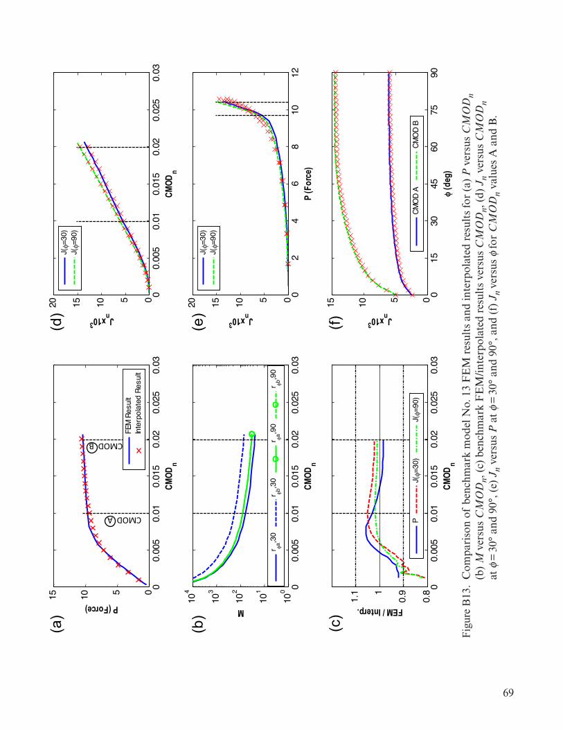
69

00.

005

0.01

0.01

50.

020.

025

0.03

051015

CMOD

n

P (Force)

FEM

Res

ult

Inte

rpol

ated

Res

ult

00.

005

0.01

0.01

50.

020.

025

0.03

05101520

CMOD

n

Jnx103

J(φ=

30)

J(φ=

90)

00.

005

0.01

0.01

50.

020.

025

0.03

100

101

102

103

104

CMOD

n

M

r φa,3

0r φb

,30

r φa,9

0r φb

,90

02

46

810

1205101520

P (F

orce

)

Jnx103

J(φ=

30)

J(φ=

90)

00.

005

0.01

0.01

50.

020.

025

0.03

0.8

0.91

1.1

CMOD

n

FEM / Interp.

PJ(φ=

30)

J(φ=

90)

015

3045

6075

90051015

φ (d

eg)

Jnx103

CMO

D A

CMO

D B

CMOD A

CMOD B

Fig. B13

(a)

(b)

(c)

(d)

(e)

(f)

Figu

re B

13.

Com

pari

son

of b

ench

mar

k m

odel

No.

13

FE

M r

esul

ts a

nd in

terp

olat

ed r

esul

ts fo

r (a

) P

ver

sus

CM

OD

n (b

) M

ver

sus

CM

OD

n, (

c) b

ench

mar

k F

EM

/inte

rpol

ated

res

ults

ver

sus

CM

OD

n, (

d) J

n ve

rsus

CM

OD

n

at f

= 3

0° a

nd 9

0°, (

e) J

n ve

rsus

P a

t f =

30°

and

90°

, and

(f)

Jn

vers

us f

for

CM

OD

n va

lues

A a

nd B

.

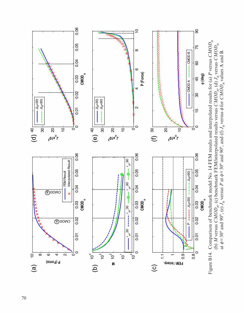
70

00.

010.

020.

030.

040.

050.

060246810

CMOD

n

P (Force)

FEM

Res

ult

Inte

rpol

ated

Res

ult

00.

010.

020.

030.

040.

050.

06010203040

CMOD

n

Jnx103

J(φ=

30)

J(φ=

90)

00.

010.

020.

030.

040.

050.

0610

0

101

102

103

104

CMOD

n

M

r φa,3

0r φb

,30

r φa,9

0r φb

,90

02

46

810

010203040

P (F

orce

)

Jnx103

J(φ=

30)

J(φ=

90)

00.

010.

020.

030.

040.

050.

060.

8

0.91

1.1

CMOD

n

FEM / Interp.

PJ(φ=

30)

J(φ=

90)

015

3045

6075

900102030

φ (d

eg)

Jnx103

CMO

D A

CMO

D B

CMOD A

CMOD B

Fig. B14

(a)

(b)

(c)

(d)

(e)

(f)

Figu

re B

14.

Com

pari

son

of b

ench

mar

k m

odel

No.

14

FE

M r

esul

ts a

nd in

terp

olat

ed r

esul

ts fo

r (a

) P

ver

sus

CM

OD

n (b

) M

ver

sus

CM

OD

n, (

c) b

ench

mar

k F

EM

/inte

rpol

ated

res

ults

ver

sus

CM

OD

n, (

d) J

n ve

rsus

CM

OD

n

at f

= 3

0° a

nd 9

0°, (

e) J

n ve

rsus

P a

t f =

30°

and

90°

, and

(f)

Jn

vers

us f

for

CM

OD

n va

lues

A a

nd B

.

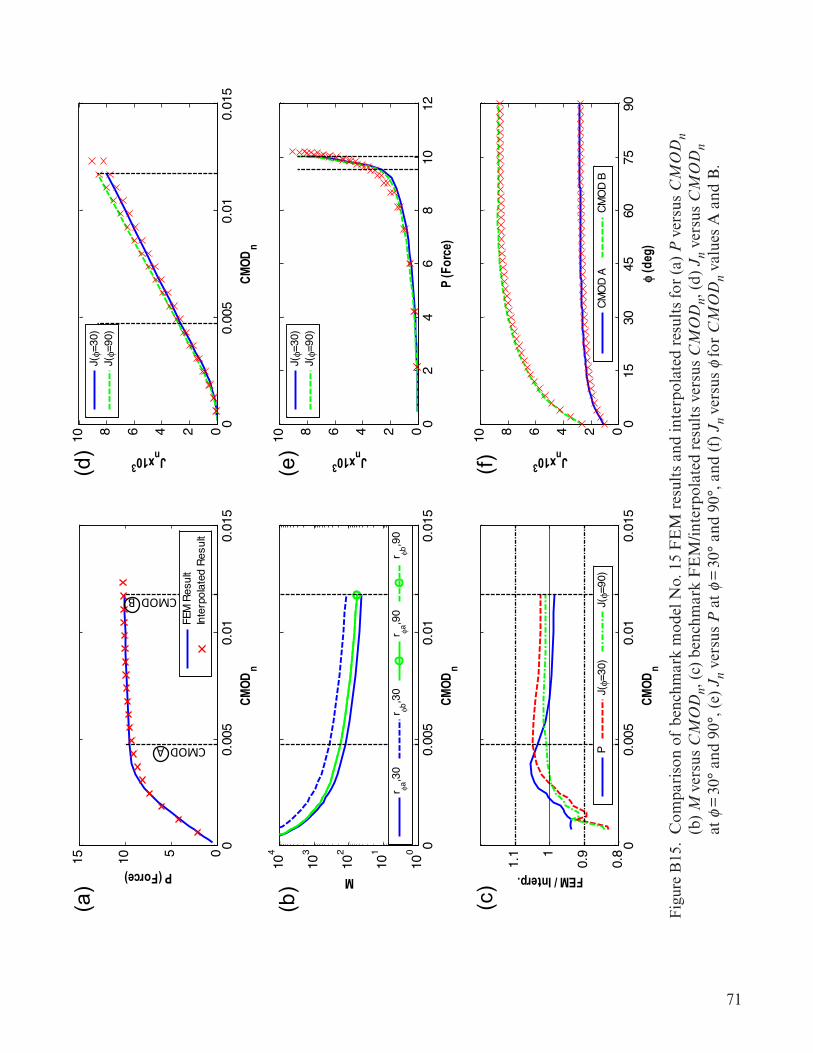
71

Figu

re B

14.

Com

pari

son

of b

ench

mar

k m

odel

No.

14

FE

M r

esul

ts a

nd in

terp

olat

ed r

esul

ts fo

r (a

) P

ver

sus

CM

OD

n (b

) M

ver

sus

CM

OD

n, (

c) b

ench

mar

k F

EM

/inte

rpol

ated

res

ults

ver

sus

CM

OD

n, (

d) J

n ve

rsus

CM

OD

n

at f

= 3

0° a

nd 9

0°, (

e) J

n ve

rsus

P a

t f =

30°

and

90°

, and

(f)

Jn

vers

us f

for

CM

OD

n va

lues

A a

nd B

.

00.

005

0.01

0.01

5051015

CMOD

n

P (Force)

FEM

Res

ult

Inte

rpol

ated

Res

ult

00.

005

0.01

0.01

50246810

CMOD

n

Jnx103

J(φ=

30)

J(φ=

90)

00.

005

0.01

0.01

510

0

101

102

103

104

CMOD

n

M

r φa,3

0r φb

,30

r φa,9

0r φb

,90

02

46

810

120246810

P (F

orce

)

Jnx103

J(φ=

30)

J(φ=

90)

00.

005

0.01

0.01

50.

8

0.91

1.1

CMOD

n

FEM / Interp.

PJ(φ=

30)

J(φ=

90)

015

3045

6075

900246810

φ (d

eg)

Jnx103

CMO

D A

CMO

D B

CMOD A

CMOD B

Fig. B15

(a)

(b)

(c)

(d)

(e)

(f)

Figu

re B

15.

Com

pari

son

of b

ench

mar

k m

odel

No.

15

FE

M r

esul

ts a

nd in

terp

olat

ed r

esul

ts fo

r (a

) P

ver

sus

CM

OD

n (b

) M

ver

sus

CM

OD

n, (

c) b

ench

mar

k F

EM

/inte

rpol

ated

res

ults

ver

sus

CM

OD

n, (

d) J

n ve

rsus

CM

OD

n

at f

= 3

0° a

nd 9

0°, (

e) J

n ve

rsus

P a

t f =

30°

and

90°

, and

(f)

Jn

vers

us f

for

CM

OD

n va

lues

A a

nd B

.

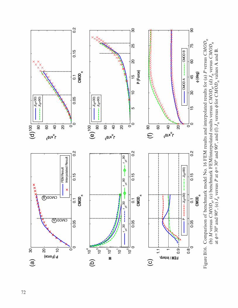
72

00.

050.

10.

150.

20102030

CMOD

n

P (Force)

FEM

Res

ult

Inte

rpol

ated

Res

ult

00.

050.

10.

150.

2020406080100

CMOD

n

Jnx103

J(φ=

30)

J(φ=

90)

00.

050.

10.

150.

210

0

101

102

103

104

CMOD

n

M

r φa,3

0r φb

,30

r φa,9

0r φb

,90

05

1015

2025

30020406080100

P (F

orce

)

Jnx103

J(φ=

30)

J(φ=

90)

00.

050.

10.

150.

20.

8

0.91

1.1

CMOD

n

FEM / Interp.

PJ(φ=

30)

J(φ=

90)

015

3045

6075

90020406080

φ (d

eg)

Jnx103

CMO

D A

CMO

D B

CMOD A

CMOD B

Fig. B16

(a)

(b)

(c)

(d)

(e)

(f)

Figu

re B

16.

Com

pari

son

of b

ench

mar

k m

odel

No.

16

FE

M r

esul

ts a

nd in

terp

olat

ed r

esul

ts fo

r (a

) P

ver

sus

CM

OD

n (b

) M

ver

sus

CM

OD

n, (

c) b

ench

mar

k F

EM

/inte

rpol

ated

res

ults

ver

sus

CM

OD

n, (

d) J

n ve

rsus

CM

OD

n

at f

= 3

0° a

nd 9

0°, (

e) J

n ve

rsus

P a

t f =

30°

and

90°

, and

(f)

Jn

vers

us f

for

CM

OD

n va

lues

A a

nd B

.

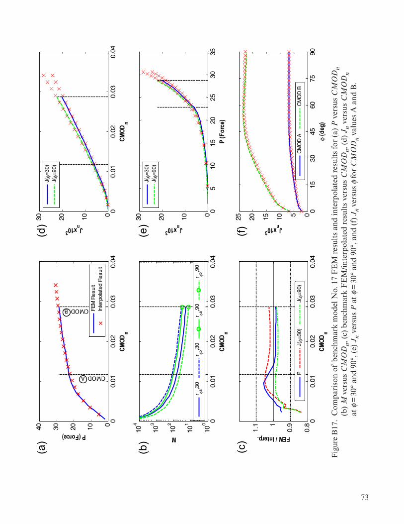
73

00.

010.

020.

030.

04010203040

CMOD

n

P (Force)

FEM

Res

ult

Inte

rpol

ated

Res

ult

00.

010.

020.

030.

040102030

CMOD

n

Jnx103

J(φ=

30)

J(φ=

90)

00.

010.

020.

030.

0410

0

101

102

103

104

CMOD

n

M

r φa,3

0r φb

,30

r φa,9

0r φb

,90

05

1015

2025

3035

0102030

P (F

orce

)

Jnx103

J(φ=

30)

J(φ=

90)

00.

010.

020.

030.

040.

8

0.91

1.1

CMOD

n

FEM / Interp.

PJ(φ=

30)

J(φ=

90)

015

3045

6075

900510152025

φ (d

eg)

Jnx103

CMO

D A

CMO

D B

CMOD A

CMOD B

Fig. B17

(a)

(b)

(c)

(d)

(e)

(f)

Figu

re B

17.

Com

pari

son

of b

ench

mar

k m

odel

No.

17

FE

M r

esul

ts a

nd in

terp

olat

ed r

esul

ts fo

r (a

) P

ver

sus

CM

OD

n (b

) M

ver

sus

CM

OD

n, (

c) b

ench

mar

k F

EM

/inte

rpol

ated

res

ults

ver

sus

CM

OD

n, (

d) J

n ve

rsus

CM

OD

n

at f

= 3

0° a

nd 9

0°, (

e) J

n ve

rsus

P a

t f =

30°

and

90°

, and

(f)

Jn

vers

us f

for

CM

OD

n va

lues

A a

nd B

.

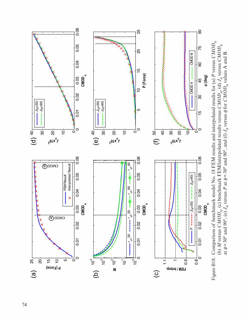
74

00.

010.

020.

030.

040.

050.

060510152025

CMOD

n

P (Force)

FEM

Res

ult

Inte

rpol

ated

Res

ult

00.

010.

020.

030.

040.

050.

06010203040

CMOD

n

Jnx103

J(φ=

30)

J(φ=

90)

00.

010.

020.

030.

040.

050.

0610

0

101

102

103

104

CMOD

n

M

r φa,3

0r φb

,30

r φa,9

0r φb

,90

05

1015

2025

010203040

P (F

orce

)

Jnx103

J(φ=

30)

J(φ=

90)

00.

010.

020.

030.

040.

050.

060.

8

0.91

1.1

CMOD

n

FEM / Interp.

PJ(φ=

30)

J(φ=

90)

015

3045

6075

9001020304050

φ (d

eg)

Jnx103

CMO

D A

CMO

D B

CMOD A

CMOD B

Fig. B18

(a)

(b)

(c)

(d)

(e)

(f)

Figu

re B

18.

Com

pari

son

of b

ench

mar

k m

odel

No.

18

FE

M r

esul

ts a

nd in

terp

olat

ed r

esul

ts fo

r (a

) P

ver

sus

CM

OD

n

(b)

M v

ersu

s C

MO

Dn,

(c)

ben

chm

ark

FE

M/in

terp

olat

ed r

esul

ts v

ersu

s C

MO

Dn,

(d)

Jn

vers

us C

MO

Dn

at

f =

30°

and

90°

, (e)

Jn

vers

us P

at

f = 3

0° a

nd 9

0°, a

nd (

f) J

n ve

rsus

f fo

r C

MO

Dn

valu

es A

and

B.

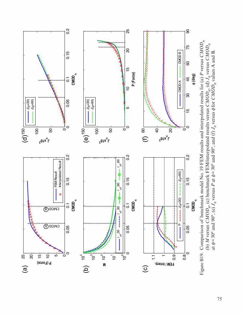
75

00.

050.

10.

150.

20510152025

CMOD

n

P (Force)

FEM

Res

ult

Inte

rpol

ated

Res

ult

00.

050.

10.

150.

2050100

150

CMOD

n

Jnx103

J(φ=

30)

J(φ=

90)

00.

050.

10.

150.

210

0

101

102

103

104

CMOD

n

M

r φa,3

0r φb

,30

r φa,9

0r φb

,90

05

1015

2025

050100

150

P (F

orce

)

Jnx103

J(φ=

30)

J(φ=

90)

00.

050.

10.

150.

20.

8

0.91

1.1

CMOD

n

FEM / Interp.

PJ(φ=

30)

J(φ=

90)

015

3045

6075

900204060

φ (d

eg)

Jnx103

CMO

D A

CMO

D B

CMOD A

CMOD B

Fig. B19

(a)

(b)

(c)

(d)

(e)

(f)

Figu

re B

19.

Com

pari

son

of b

ench

mar

k m

odel

No.

19

FE

M r

esul

ts a

nd in

terp

olat

ed r

esul

ts fo

r (a

) P

ver

sus

CM

OD

n (b

) M

ver

sus

CM

OD

n, (

c) b

ench

mar

k F

EM

/inte

rpol

ated

res

ults

ver

sus

CM

OD

n, (

d) J

n ve

rsus

CM

OD

n

at f

= 3

0° a

nd 9

0°, (

e) J

n ve

rsus

P a

t f =

30°

and

90°

, and

(f)

Jn

vers

us f

for

CM

OD

n va

lues

A a

nd B

.

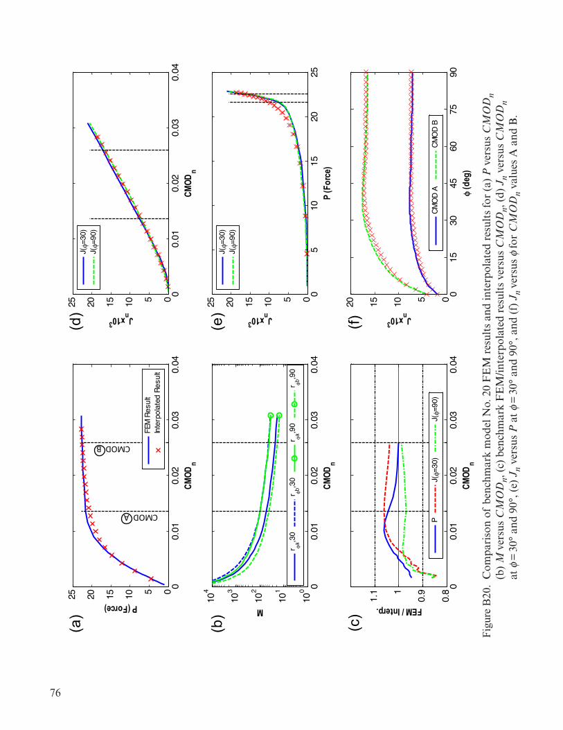
76

00.

010.

020.

030.

040510152025

CMOD

n

P (Force)

FEM

Res

ult

Inte

rpol

ated

Res

ult

00.

010.

020.

030.

040510152025

CMOD

n

Jnx103

J(φ=

30)

J(φ=

90)

00.

010.

020.

030.

0410

0

101

102

103

104

CMOD

n

M

r φa,3

0r φb

,30

r φa,9

0r φb

,90

05

1015

2025

0510152025

P (F

orce

)

Jnx103

J(φ=

30)

J(φ=

90)

00.

010.

020.

030.

040.

8

0.91

1.1

CMOD

n

FEM / Interp.

PJ(φ=

30)

J(φ=

90)

015

3045

6075

9005101520

φ (d

eg)

Jnx103

CMO

D A

CMO

D B

CMOD A

CMOD B

Fig. B20

(a)

(b)

(c)

(d)

(e)

(f)

Figu

re B

20.

Com

pari

son

of b

ench

mar

k m

odel

No.

20

FE

M r

esul

ts a

nd in

terp

olat

ed r

esul

ts fo

r (a

) P

ver

sus

CM

OD

n (b

) M

ver

sus

CM

OD

n, (

c) b

ench

mar

k F

EM

/inte

rpol

ated

res

ults

ver

sus

CM

OD

n, (

d) J

n ve

rsus

CM

OD

n

at f

= 3

0° a

nd 9

0°, (

e) J

n ve

rsus

P a

t f =

30°

and

90°

, and

(f)

Jn

vers

us f

for

CM

OD

n va

lues

A a

nd B

.

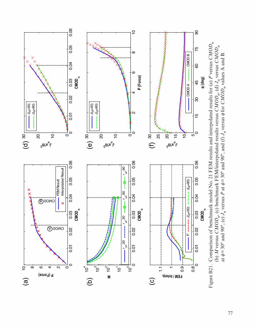
77

00.

010.

020.

030.

040.

050.

060246810

CMOD

n

P (Force)

FEM

Res

ult

Inte

rpol

ated

Res

ult

00.

010.

020.

030.

040.

050.

060102030

CMOD

n

Jnx103

J(φ=

30)

J(φ=

90)

00.

010.

020.

030.

040.

050.

0610

0

101

102

103

104

CMOD

n

M

r φa,3

0r φb

,30

r φa,9

0r φb

,90

02

46

810

0102030

P (F

orce

)

Jnx103

J(φ=

30)

J(φ=

90)

00.

010.

020.

030.

040.

050.

060.

8

0.91

1.1

CMOD

n

FEM / Interp.

PJ(φ=

30)

J(φ=

90)

015

3045

6075

9051015202530

φ (d

eg)

Jnx103

CMO

D A

CMO

D B

CMOD A

CMOD B

Fig. B21

(a)

(b)

(c)

(d)

(e)

(f)

Figu

re B

21.

Com

pari

son

of b

ench

mar

k m

odel

No.

21

FE

M r

esul

ts a

nd in

terp

olat

ed r

esul

ts fo

r (a

) P

ver

sus

CM

OD

n (b

) M

ver

sus

CM

OD

n, (

c) b

ench

mar

k F

EM

/inte

rpol

ated

res

ults

ver

sus

CM

OD

n, (

d) J

n ve

rsus

CM

OD

n

at f

= 3

0° a

nd 9

0°, (

e) J

n ve

rsus

P a

t f =

30°

and

90°

, and

(f)

Jn

vers

us f

for

CM

OD

n va

lues

A a

nd B

.

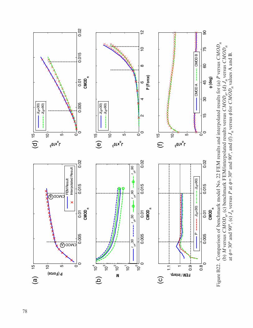
78

00.

005

0.01

0.01

50.

02051015

CMOD

n

P (Force)

FEM

Res

ult

Inte

rpol

ated

Res

ult

00.

005

0.01

0.01

50.

02051015

CMOD

n

Jnx103

J(φ=

30)

J(φ=

90)

00.

005

0.01

0.01

50.

0210

0

101

102

103

104

CMOD

n

M

r φa,3

0r φb

,30

r φa,9

0r φb

,90

02

46

810

12051015

P (F

orce

)

Jnx103

J(φ=

30)

J(φ=

90)

00.

005

0.01

0.01

50.

020.

8

0.91

1.1

CMOD

n

FEM / Interp.

PJ(φ=

30)

J(φ=

90)

015

3045

6075

90051015

φ (d

eg)

Jnx103

CMO

D A

CMO

D B

CMOD A

CMOD B

Fig. B22

(a)

(b)

(c)

(d)

(e)

(f)

Figu

re B

22.

Com

pari

son

of b

ench

mar

k m

odel

No.

22

FE

M r

esul

ts a

nd in

terp

olat

ed r

esul

ts fo

r (a

) P

ver

sus

CM

OD

n (b

) M

ver

sus

CM

OD

n, (

c) b

ench

mar

k F

EM

/inte

rpol

ated

res

ults

ver

sus

CM

OD

n, (

d) J

n ve

rsus

CM

OD

n

at f

= 3

0° a

nd 9

0°, (

e) J

n ve

rsus

P a

t f =

30°

and

90°

, and

(f)

Jn

vers

us f

for

CM

OD

n va

lues

A a

nd B

.

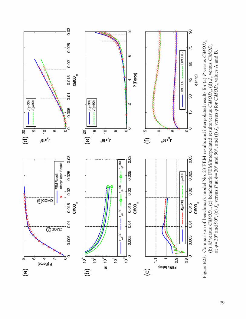
79

Figu

re B

22.

Com

pari

son

of b

ench

mar

k m

odel

No.

22

FE

M r

esul

ts a

nd in

terp

olat

ed r

esul

ts fo

r (a

) P

ver

sus

CM

OD

n (b

) M

ver

sus

CM

OD

n, (

c) b

ench

mar

k F

EM

/inte

rpol

ated

res

ults

ver

sus

CM

OD

n, (

d) J

n ve

rsus

CM

OD

n

at f

= 3

0° a

nd 9

0°, (

e) J

n ve

rsus

P a

t f =

30°

and

90°

, and

(f)

Jn

vers

us f

for

CM

OD

n va

lues

A a

nd B

.

00.

005

0.01

0.01

50.

020.

025

0.03

02468

CMOD

n

P (Force)

FEM

Res

ult

Inte

rpol

ated

Res

ult

00.

005

0.01

0.01

50.

020.

025

0.03

05101520

CMOD

n

Jnx103

J(φ=

30)

J(φ=

90)

00.

005

0.01

0.01

50.

020.

025

0.03

100

101

102

103

104

CMOD

n

M

r φa,3

0r φb

,30

r φa,9

0r φb

,90

02

46

805101520

P (F

orce

)

Jnx103

J(φ=

30)

J(φ=

90)

00.

005

0.01

0.01

50.

020.

025

0.03

0.8

0.91

1.1

CMOD

n

FEM / Interp.

PJ(φ=

30)

J(φ=

90)

015

3045

6075

90051015

φ (d

eg)

Jnx103

CMO

D A

CMO

D B

CMOD A

CMOD B

Fig. B23

(a)

(b)

(c)

(d)

(e)

(f)

Figu

re B

23.

Com

pari

son

of b

ench

mar

k m

odel

No.

23

FE

M r

esul

ts a

nd in

terp

olat

ed r

esul

ts fo

r (a

) P

ver

sus

CM

OD

n (b

) M

ver

sus

CM

OD

n, (

c) b

ench

mar

k F

EM

/inte

rpol

ated

res

ults

ver

sus

CM

OD

n, (

d) J

n ve

rsus

CM

OD

n

at f

= 3

0° a

nd 9

0°, (

e) J

n ve

rsus

P a

t f =

30°

and

90°

, and

(f)

Jn

vers

us f

for

CM

OD

n va

lues

A a

nd B

.

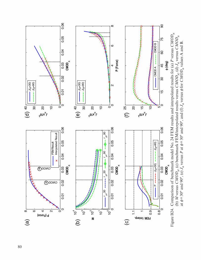
80

00.

010.

020.

030.

040.

050.

0602468

CMOD

n

P (Force)

FEM

Res

ult

Inte

rpol

ated

Res

ult

00.

010.

020.

030.

040.

050.

06010203040

CMOD

n

Jnx103

J(φ=

30)

J(φ=

90)

00.

010.

020.

030.

040.

050.

0610

0

101

102

103

104

CMOD

n

M

r φa,3

0r φb

,30

r φa,9

0r φb

,90

02

46

8010203040

P (F

orce

)

Jnx103

J(φ=

30)

J(φ=

90)

00.

010.

020.

030.

040.

050.

060.

8

0.91

1.1

CMOD

n

FEM / Interp.

PJ(φ=

30)

J(φ=

90)

015

3045

6075

90510152025

φ (d

eg)

Jnx103

CMO

D A

CMO

D B

CMOD A

CMOD B

Fig. B24

(a)

(b)

(c)

(d)

(e)

(f)

Figu

re B

24.

Com

pari

son

of b

ench

mar

k m

odel

No.

24

FE

M r

esul

ts a

nd in

terp

olat

ed r

esul

ts fo

r (a

) P

ver

sus

CM

OD

n (b

) M

ver

sus

CM

OD

n, (

c) b

ench

mar

k F

EM

/inte

rpol

ated

res

ults

ver

sus

CM

OD

n, (

d) J

n ve

rsus

CM

OD

n

at f

= 3

0° a

nd 9

0°, (

e) J

n ve

rsus

P a

t f =

30°

and

90°

, and

(f)

Jn

vers

us f

for

CM

OD

n va

lues

A a

nd B

.

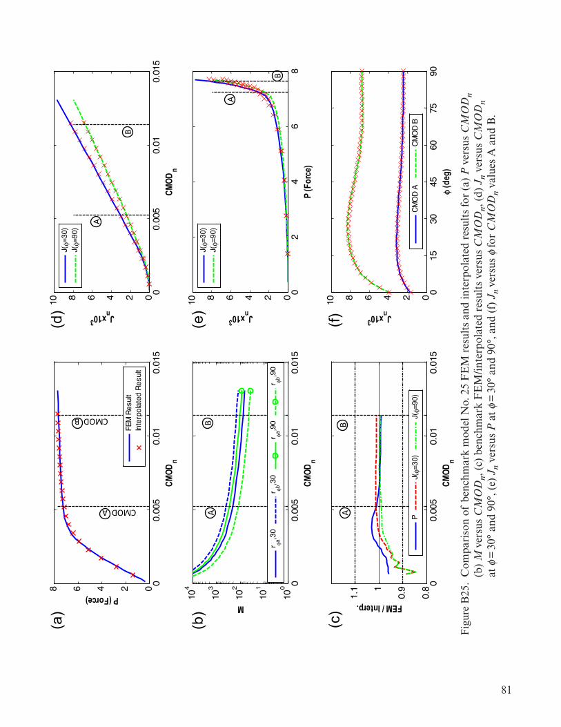
81

Figu

re B

24.

Com

pari

son

of b

ench

mar

k m

odel

No.

24

FE

M r

esul

ts a

nd in

terp

olat

ed r

esul

ts fo

r (a

) P

ver

sus

CM

OD

n (b

) M

ver

sus

CM

OD

n, (

c) b

ench

mar

k F

EM

/inte

rpol

ated

res

ults

ver

sus

CM

OD

n, (

d) J

n ve

rsus

CM

OD

n

at f

= 3

0° a

nd 9

0°, (

e) J

n ve

rsus

P a

t f =

30°

and

90°

, and

(f)

Jn

vers

us f

for

CM

OD

n va

lues

A a

nd B

.

00.

005

0.01

0.01

502468

CMOD

n

P (Force)

FEM

Res

ult

Inte

rpol

ated

Res

ult

00.

005

0.01

0.01

50246810

CMOD

n

Jnx103

J(φ=

30)

J(φ=

90)

00.

005

0.01

0.01

510

0

101

102

103

104

CMOD

n

M

r φa,3

0r φb

,30

r φa,9

0r φb

,90

02

46

80246810

P (F

orce

)

Jnx103

J(φ=

30)

J(φ=

90)

00.

005

0.01

0.01

50.

8

0.91

1.1

CMOD

n

FEM / Interp.

PJ(φ=

30)

J(φ=

90)

015

3045

6075

900246810

φ (d

eg)

Jnx103

CMO

D A

CMO

D B

Fig. B25

CMOD A

CMOD B

AB

AB

A

B

A

B

(a)

(b)

(c)

(d)

(e)

(f)

Figu

re B

25.

Com

pari

son

of b

ench

mar

k m

odel

No.

25

FE

M r

esul

ts a

nd in

terp

olat

ed r

esul

ts fo

r (a

) P

ver

sus

CM

OD

n (b

) M

ver

sus

CM

OD

n, (

c) b

ench

mar

k F

EM

/inte

rpol

ated

res

ults

ver

sus

CM

OD

n, (

d) J

n ve

rsus

CM

OD

n

at f

= 3

0° a

nd 9

0°, (

e) J

n ve

rsus

P a

t f =

30°

and

90°

, and

(f)

Jn

vers

us f

for

CM

OD

n va

lues

A a

nd B

.

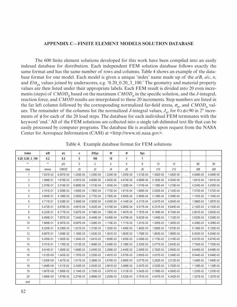
82

APPENDIX C—FINITE ELEMENT MODELS SOLUTION DATABASE

The 600 finite element solutions developed for this work have been compiled into an easily indexed database for distribution. Each independent FEM solution database follows exactly the same format and has the same number of rows and columns. Table 4 shows an example of the data-base format for one model. Each model is given a unique ‘index’ name made up of the a/B, a/c, n, and E/sys values joined by underscores, e.g. ‘0.20_0.20_3_100.’ The geometry and material property values are then listed under their appropriate labels. Each FEM result is divided into 20 even incre-ments (steps) of CMODn based on the maximum CMODn in the specific solution, and the J-integral, reaction force, and CMOD results are interpolated to these 20 increments. Step numbers are listed in the far left column followed by the corresponding normalized far-field stress, sn, and CMODn val-ues. The remainder of the columns list the normalized J-integral values, Jn, for 0 ≥ f ≥ 90 in 2° incre-ments of f for each of the 20 load steps. The database for each individual FEM terminates with the keyword ‘end.’ All of the FEM solutions are collected into a single tab delimited text file that can be easily processed by computer programs. The database file is available upon request from the NASA Center for Aerospace Information (CASI) at <http://www.sti.nasa.gov>.

Table 4. Example database format for FEM solutions

Index a/B a/c n E/Sys W B Sys0.20_0.20_3_100 0.2 0.2 3 100 10 1 1

** ** phi 0 2 4 6 8 10 12 … 88 90step stress CMOD J0 J2 J4 J6 J8 J10 J12 … J88 J90

1 7.937E-02 8.397E-04 1.240E-05 1.235E-05 1.224E-05 1.255E-05 1.313E-05 1.392E-05 1.492E-05 … 4.948E-05 4.949E-052 1.586E-01 1.679E-03 4.581E-05 4.606E-05 4.562E-05 4.674E-05 4.889E-05 5.182E-05 5.554E-05 … 1.841E-04 1.841E-043 2.376E-01 2.519E-03 9.888E-05 1.013E-04 1.004E-04 1.028E-04 1.074E-04 1.138E-04 1.219E-04 … 4.034E-04 4.035E-044 3.161E-01 3.359E-03 1.695E-04 1.780E-04 1.772E-04 1.811E-04 1.890E-04 2.000E-04 2.142E-04 … 7.070E-04 7.072E-045 3.940E-01 4.198E-03 2.565E-04 2.772E-04 2.790E-04 2.850E-04 2.969E-04 3.138E-04 3.356E-04 … 1.103E-03 1.104E-036 4.711E-01 5.038E-03 3.566E-04 3.955E-04 4.045E-04 4.144E-04 4.311E-04 4.547E-04 4.854E-04 … 1.586E-03 1.587E-037 5.472E-01 5.878E-03 4.681E-04 5.302E-04 5.516E-04 5.685E-04 5.917E-04 6.231E-04 6.640E-04 … 2.152E-03 2.153E-038 6.222E-01 6.717E-03 5.907E-04 6.798E-04 7.185E-04 7.467E-04 7.787E-04 8.199E-04 8.724E-04 … 2.801E-03 2.802E-039 6.956E-01 7.557E-03 7.244E-04 8.449E-04 9.046E-04 9.479E-04 9.923E-04 1.046E-03 1.112E-03 … 3.525E-03 3.526E-03

10 7.669E-01 8.397E-03 8.697E-04 1.026E-03 1.110E-03 1.171E-03 1.231E-03 1.300E-03 1.383E-03 … 4.306E-03 4.308E-0311 8.320E-01 9.236E-03 1.021E-03 1.215E-03 1.325E-03 1.406E-03 1.482E-03 1.569E-03 1.670E-03 … 5.148E-03 5.150E-0312 8.887E-01 1.008E-02 1.185E-03 1.423E-03 1.561E-03 1.663E-03 1.758E-03 1.863E-03 1.985E-03 … 6.002E-03 6.004E-0313 9.355E-01 1.092E-02 1.354E-03 1.641E-03 1.809E-03 1.935E-03 2.049E-03 2.175E-03 2.319E-03 … 6.872E-03 6.874E-0314 9.701E-01 1.176E-02 1.513E-03 1.848E-03 2.046E-03 2.196E-03 2.330E-03 2.477E-03 2.643E-03 … 7.754E-03 7.755E-0315 9.914E-01 1.260E-02 1.658E-03 2.040E-03 2.268E-03 2.440E-03 2.595E-03 2.762E-03 2.950E-03 … 8.646E-03 8.648E-0316 1.012E+00 1.343E-02 1.797E-03 2.225E-03 2.481E-03 2.675E-03 2.850E-03 3.037E-03 3.246E-03 … 9.544E-03 9.546E-0317 1.030E+00 1.427E-02 1.917E-03 2.389E-03 2.670E-03 2.885E-03 3.077E-03 3.282E-03 3.512E-03 … 1.046E-02 1.046E-0218 1.048E+00 1.511E-02 2.035E-03 2.553E-03 2.861E-03 3.096E-03 3.307E-03 3.532E-03 3.783E-03 … 1.138E-02 1.139E-0219 1.067E+00 1.595E-02 2.154E-03 2.720E-03 3.057E-03 3.313E-03 3.542E-03 3.788E-03 4.060E-03 … 1.233E-02 1.233E-0220 1.086E+00 1.679E-02 2.274E-03 2.889E-03 3.255E-03 3.532E-03 3.781E-03 4.047E-03 4.342E-03 … 1.327E-02 1.327E-02

end

83

APPENDIX D—BENCHMARK FINITE ELEMENT MODELS SOLUTION DATABASE

The 25 benchmark finite element solutions developed for this work have been complied into an easily indexed database for distribution. The solution database follows the same format as the 600 model FEM database described in appendix C. The database file is available upon request from the NASA Center for Aerospace Information (CASI) at <http://www.sti.nasa.gov>.

84

REFERENCES

1. FEACrack, Quest Integrity Group, <http://www.questintegrity.com/products/feacrack-3D- crack-mesh-software/>, Verified December 12, 2012.

2. ABAQUS/CAE, Dassault Systèmes. <http://www.3ds.com/products/simulia/portfolio/abaqus/abaqus-portfolio/abaquscae/>, Verified January 16, 2013.

3. Newman, J.C.; and Raju, I.S.: Stress-Intensity Factor Equations for Cracks in Three-Dimen-sional Finite Bodies Subjected to Tension and Bending Loads, NASA/TM—1984–85793, Langley Research Center, VA, April 1984.

4. Newman, J.C.; Reuter, W.G.; and Aveline, C.R.: “Stress and Fracture Analyses of Semi-Ellip-tical Surface Cracks,” Fatigue and Fracture Mechanics, P.C. Harris and K.L. Jerina (eds.), American Society of Testing and Materials, West Conshohocken, PA, Vol. 30, pp. 403–423, January 2000.

5. NASGRO, Southwest Research Institute, <http://www.swri.org/4org/d18/mateng/matint/nas-gro/default.htm>, Verified January 16, 2013.

6. McClung, R.C.; Chell, G.G.; Lee, Y.D.; et al.: Development of a Practical Methodology for Elastic-Plastic and Fully Plastic Fatigue Crack Growth, NASA/CR—1999–209428, Marshall Space Flight Center, AL, July 1999.

7. Anderson, T.L.: Fracture Mechanics: Fundamentals and Applications, 3rd ed., CRC Press, Boca Raton, FL, 2005.

8. Kumar, V.; German, M.D.; and Shih, C.F.: An Engineering Approach for Elastic-Plastic Fracture Analysis, Tech. Rep. NP-1931, Electric Power Research Institute, Schenectady, NY, July 1981.

9. Kumar, V.; German, M.D.; Wilkening, W.W.; et al.: Advances in Elastic-Plastic Fracture Analy-sis, Tech. Rep. NP-3607, Electric Power Research Institute, Schenectady, NY, August 1984.

10. Kumar, V.; and German, M.D.: Elastic-Plastic Fracture Analysis of Through-Wall and Surface Flaws in Cylinders, Tech. Rep. NP-5596, Electric Power Research Institute, Schenectady, NY, January 1988.

11. Ainsworth, R.A.: “The assessment of defects in structures of strain hardening material,” Engi-neering Fracture Mechanics, Vol. 19, No. 4, pp. 633–642, 1984.

85

12. Ramberg, W.; and Osgood, W.R.: Description of Stress-Strain Curves by Three-Parameters, Technical Note 902, National Advisory Committee on Aeronautics, Washington, DC, April 1943.

13. Yagawa, G.; Yasumi, K.; and Hiroyoshi, U.: “Three-dimensional fully plastic solutions for semi-elliptical surface cracks,” International Journal of Pressure Vessels and Piping, Vol. 53, No. 3, pp. 457–510, 1993.

14. Wilson, C.D.; and Natarajan, K.R.: Verification of NASGRO Elastic-Plastic Modules: J-Inte-gral Computation, MCTR-03-03-01, Center for Manufacturing Research, Tennessee Techno-logical University, TN, 2003.

15. Wang, X.: “Fully plastic J-integral solutions for surface cracked plates under biaxial loading,” Engineering Fracture Mechanics, Vol. 73, No. 11, pp. 1581–1595, March 2006.

16. Kim, Y.J.; Shim, D.J.; Choi, J.B.; and Young, J.K.: “Approximate J estimates for tension-loaded plates with semi-elliptical surface cracks,” Engineering Fracture Mechanics, Vol. 69, No. 13, pp. 1447–1463, September 2002.

17. Wells, D.N.; and Allen, P.A.: Analytical Round Robin for Elastic-Plastic Analysis of Surface Cracked Plates: Phase I Results, NASA/TM—2012–217456, Marshall Space Flight Center, AL, March 2012.

18. WARP3D, Static and Dynamic Nonlinear Analysis of Fracture in Solids, Dodds, R.H., Uni-versity of Illinois at Urbana-Champaign, <http://code.google.com/p/warp3d/>, Verified December 12, 2012.

19. Matlab, Mathworks, <http://www.mathworks.com/products/matlab/>, Verified December 12, 2012.

20. Brocks, W.; and Scheider, I.: “Reliable J-Values: Numerical aspects of the path-dependence of the J-integral in incremental plasticity,” Materialprüfung, Vol. 45, No. 6, pp. 264 –275, 2003.

86

REPORT DOCUMENTATION PAGE Form ApprovedOMB No. 0704-0188

The public reporting burden for this collection of information is estimated to average 1 hour per response, including the time for reviewing instructions, searching existing data sources, gathering and maintaining the data needed, and completing and reviewing the collection of information. Send comments regarding this burden estimate or any other aspect of this collection of information, including suggestions for reducing this burden, to Department of Defense, Washington Headquarters Services, Directorate for Information Operation and Reports (0704-0188), 1215 Jefferson Davis Highway, Suite 1204, Arlington, VA 22202-4302. Respondents should be aware that notwithstanding any other provision of law, no person shall be subject to any penalty for failing to comply with a collection of information if it does not display a currently valid OMB control number.PLEASE DO NOT RETURN YOUR FORM TO THE ABOVE ADDRESS.

1. REPORT DATE (DD-MM-YYYY) 2. REPORT TYPE 3. DATES COVERED (From - To)

4. TITLE AND SUBTITLE 5a. CONTRACT NUMBER

5b. GRANT NUMBER

5c. PROGRAM ELEMENT NUMBER

6. AUTHOR(S) 5d. PROJECT NUMBER

5e. TASK NUMBER

5f. WORK UNIT NUMBER

7. PERFORMING ORGANIZATION NAME(S) AND ADDRESS(ES) 8. PERFORMING ORGANIZATION REPORT NUMBER

9. SPONSORING/MONITORING AGENCY NAME(S) AND ADDRESS(ES) 10. SPONSORING/MONITOR’S ACRONYM(S)

11. SPONSORING/MONITORING REPORT NUMBER

12. DISTRIBUTION/AVAILABILITY STATEMENT

13. SUPPLEMENTARY NOTES

14. ABSTRACT

15. SUBJECT TERMS

16. SECURITY CLASSIFICATION OF:a. REPORT b. ABSTRACT c. THIS PAGE

17. LIMITATION OF ABSTRACT 18. NUMBER OF PAGES

19a. NAME OF RESPONSIBLE PERSON

19b. TELEPHONE NUMBER (Include area code)

Standard Form 298 (Rev. 8-98)Prescribed by ANSI Std. Z39-18

Elastic-Plastic J-Integral Solutions for Surface Cracks in Tension Using an Interpolation Methodology

P.A. Allen and D.N. Wells

George C. Marshall Space Flight CenterHuntsville, AL 35812

National Aeronautics and Space AdministrationWashington, DC 20546–0001

Unclassified-UnlimitedSubject Category 39Availability: NASA CASI (443–757–5802)

Prepared by the Materials and Processes Laboratory, Engineering DirectorateSupplemental database files available upon request.

M–1356

Technical Publication

NASA/TP—2013–217480

structural mechanics, metals and metallic materials

01–04–2013

UU 104

NASA

U U U

No closed form solutions exist for the elastic-plastic J-integral for surface cracks due to the nonlinear, three-dimensional nature of the problem. Traditionally, each surface crack must be analyzed with a unique and time-consuming nonlinear finite element analysis. To overcome this shortcoming, the authors have developed and analyzed an array of 600 3D nonlinear finite element models for surface cracks in flat plates under tension loading. The solution space covers a wide range of crack shapes and depths (shape: 0.2 ≤ a/c ≤ 1, depth: 0.2 ≤ a/B ≤ 0.8) and material flow properties (elastic modulus-to-yield ratio: 100 ≤ E/ys ≤ 1,000, and hard-ening: 3 ≤ n ≤ 20). The authors have developed a methodology for interpolating between the goemetric and material property vari-ables that allows the user to reliably evaluate the full elastic-plastic J-integral and force versus crack mouth opening displacement solution; thus, a solution can be obtained very rapidly by users without elastic-plastic fracture mechanics modeling experience. Complete solutions for the 600 models and 25 additional benchmark models are provided in tabular format.

STI Help Desk at email: [email protected]

STI Help Desk at: 443–757–5802

The NASA STI Program…in Profile

Since its founding, NASA has been dedicated to the advancement of aeronautics and space science. The NASA Scientific and Technical Information (STI) Program Office plays a key part in helping NASA maintain this important role.

The NASA STI Program Office is operated by Langley Research Center, the lead center for NASA’s scientific and technical information. The NASA STI Program Office provides access to the NASA STI Database, the largest collection of aeronautical and space science STI in the world. The Program Office is also NASA’s institutional mechanism for disseminating the results of its research and development activities. These results are published by NASA in the NASA STI Report Series, which includes the following report types:

• TECHNICAL PUBLICATION. Reports of completed research or a major significant phase of research that present the results of NASA programs and include extensive data or theoretical analysis. Includes compilations of significant scientific and technical data and information deemed to be of continuing reference value. NASA’s counterpart of peer-reviewed formal professional papers but has less stringent limitations on manuscript length and extent of graphic presentations.

• TECHNICAL MEMORANDUM. Scientific and technical findings that are preliminary or of specialized interest, e.g., quick release reports, working papers, and bibliographies that contain minimal annotation. Does not contain extensive analysis.

• CONTRACTOR REPORT. Scientific and technical findings by NASA-sponsored contractors and grantees.

• CONFERENCE PUBLICATION. Collected papers from scientific and technical conferences, symposia, seminars, or other meetings sponsored or cosponsored by NASA.

• SPECIAL PUBLICATION. Scientific, technical, or historical information from NASA programs, projects, and mission, often concerned with subjects having substantial public interest.

• TECHNICAL TRANSLATION. English-language translations of foreign

scientific and technical material pertinent to NASA’s mission.

Specialized services that complement the STI Program Office’s diverse offerings include creating custom thesauri, building customized databases, organizing and publishing research results…even providing videos.

For more information about the NASA STI Program Office, see the following:

• Access the NASA STI program home page at <http://www.sti.nasa.gov>

• E-mail your question via the Internet to <[email protected]>

• Fax your question to the NASA STI Help Desk at 443 –757–5803

• Phone the NASA STI Help Desk at 443 –757–5802

• Write to: NASA STI Help Desk NASA Center for AeroSpace Information 7115 Standard Drive Hanover, MD 21076–1320

NASA/TP—2013–


March 2013

National Aeronautics andSpace AdministrationIS20George C. Marshall Space Flight CenterHuntsville, Alabama 35812

Elastic-Plastic J-Integral Solutions for Surface Cracks in ...Elastic-Plastic J-Integral Solutions...

Documents

Transcript of Elastic-Plastic J-Integral Solutions for Surface Cracks in ...Elastic-Plastic J-Integral Solutions...