ELASTIC DEFORMATIONS OF COMPACT...

arX

iv:1

402.

6634

v1 [

gr-q

c] 2

6 Fe

b 20

14

ELASTIC DEFORMATIONS OF COMPACT STARS

LARS ANDERSSON†, ROBERT BEIG‡, AND BERND G. SCHMIDT

Abstract. We prove existence of solutions for an elastic body interactingwith itself through its Newtonian gravitational field. Our construction worksfor configurations near one given by a self-gravitating ball of perfect fluid.We use an implicit function argument. In so doing we have to revisit someclassical work in the astrophysical literature concerning linear stability ofperfect fluid stars. The results presented here extend previous work by theauthors, which was restricted to the astrophysically insignificant situationof configurations near one of vanishing stress. In particular, “mountains onneutron stars”, which are made possible by the presence of an elastic crustin neutron stars, can be treated using the techniques developed here.

1. Introduction

The matter models commonly used to describe stars in astrophysics are fluids.By a classical result of Lichtenstein [13], a self-gravitating time-independentfluid body is spherically symmetric in the absence of rotation. However, due tothe presence of a solid crust, it is possible for neutron stars to carry mountains(see [9]). In view of the result of Lichtenstein, in order to describe somethinglike “mountains on a neutron star” it is necessary to consider matter modelswhich allow non-isotropic stresses, for example those of elasticity theory.

The currently known existence results for non-spherical self-gravitating time-indepent elastic bodies deal with deformations of a relaxed stress-free state. In[5] it was shown that for a small body for which a relaxed stress-free configura-tion exists, there is a unique nearby solution which describes the deformationof the body under its own Newtonian gravitational field. The analogous resultin Einstein gravity was given in [3]. However, a large self-gravitating object likea neutron stars does not admit a relaxed configuration. This is the situationwhich we shall consider in this paper.

In section 2, we give an outline of the formalism of elasticity used in thispaper, following [2], and specializing to the time-independent case. Given areference body, i.e., a domain in three-dimensional Euclidean body space thephysical body is its image in physical space under a deformation map. Thefield theoretic description of the material in terms of deformation maps givesthe material frame (or Lagrangian) form of the theory, while the descriptionin terms of the inverses of the deformation maps, called configuration maps,taking the physical body to the reference body, gives the Eulerian picture. Thefield equations for Newtonian elasticity can be derived from an action principle

Date: February 26, 2014.‡ Supported in part by Fonds zur Forderung der Wissenschaftlichen Forschung project no.

P20414-N16.

1

http://arxiv.org/abs/1402.6634v1

2 L. ANDERSSON, R. BEIG, AND B. SCHMIDT

in which the properties of the matter are defined by a “stored energy function”which depends on the configuration, and a Riemannian reference metric on thebody, called the body metric. The body metric is taken to be conformal tothe Euclidean metric with the conformal factor chosen so that the associatedvolume element is that given by the particle number density of the referenceconfiguration, see below. This is done in section 3, working in the Euleriansetting. We consider here only isotropic materials, for which the stored energydepends on the configuration map only via the three principal invariants of thestrain tensor1 defined with respect to the body metric.

The resulting Euler-Lagrange equations for a self-gravitating elastic bodyform a quasi-linear, integro-differential boundary value problem for the config-uration map, with an a priori unknown boundary given by the condition thatthe normal stress be zero there. In section 3.3, we reformulate the system in thematerial frame, as a system of equations on the reference body, i.e. a fixed do-main in Euclidean space. The system of equations on the body given in section3.3 replaces the free boundary of the physical body, by the fixed boundary ofthe reference body, with a Neumann type boundary condition. For a large classof stored energy functions we obtain by this procedure a quasilinear elliptic,integro-differential boundary value problem, the solutions of which representself-gravitating time-independent elastic bodies.

There is no general existence theorem in the literature which can be ap-plied to such systems, except in the spherically symmetric case. A minimizerfor the variational problem describing a Newtonian self-gravitating body hasbeen shown to exist, under certain conditions, in [8]. However, it is unknownunder what conditions this minimizer satisfies the Euler-Lagrange equations.Specializing to the spherically symmetric case, the field equations for a self-gravitating, time-independent body reduces to a system of ordinary differentialequations, for which existence of solutions is easier to show. For example, inthe case of perfect fluid matter, which we will use as background, as explainedbelow, there is a simple condition on the equation of state (see [17] for therelativistic case, the Newtonian case is analogous) guaranteeing existence of so-lutions corresponding to a finite body. We shall in this paper construct “large”non-spherical time-independent self-gravitating bodies by applying the implicitfunction theorem to deform appropriate spherical background solutions.

We choose our reference configuration as follows, see sections 3.4, 3.5 fordetails. As mentioned above, a Newtonian self-gravitating fluid body is spher-ically symmetric. In fact, a fluid body centered at the origin is determined byspecifying its stored energy e(ρ) (in the context of fluids usually referred to asinternal energy) as a function of the physical density ρ of the fluid, togetherwith its central density, see again [17]. The fluid density ρ can be taken as oneof the principal invariants of the strain tensor.

Keeping these facts in mind, a time-independent self-gravitating fluid bodywith support of finite radius, and non-vanishing density at the boundary, canbe viewed as a special case of an elastic material, with deformation map given

1The strain tensor is the push-forward of the contravariant form of the metric on space,which in the present setting can be taken to be the Euclidean metric.

ELASTIC DEFORMATIONS OF COMPACT STARS 3

by the identity, and with spatial density ρ. A body metric conformal to theEuclidean metric is then chosen, which has volume element equal to ρ. Thetwo remaining principal invariants of the strain tensor are represented in termsof expressions τ, δ which vanish at this background configuration, cf. [18] forrelated definitions. We then choose a stored energy function which coincideswith e(ρ) at the reference configuration, but which has elastic stresses for non-spherical configurations. The just described elastic body is then taken as thestarting point of an implicit function theorem argument.

Given the stored energy as a function of the principal invariants, the actionand hence also the Euler-Lagrange equations are specified. We introduce a1-parameter family of non-spherical body densities ρλ with ρ0 = ρ, the spheri-cally symmetric density of the reference body. Introducing a suitable setting interms of Sobolev spaces, see section 4, we can formulate the system of Euler-Lagrange equations in the material frame as a 1-parameter family of non-linearfunctional equations F [ρλ, φλ] = 0. Our problem is then reduced to showingthat deformation maps φλ solving this equation exist for small λ 6= 0.

In order to apply the implicit function theorem to construct such solutions,we must analyze the Frechet derivative of the F or equivalently the equationslinearized at the reference deformation. This is done in section 5, which formsthe core of the paper. We start by calculating the linearized operator. Theresult is (5.3). With our choice of stored energy, the first variation of theaction is “pure fluid” (which is why the identity map is a solution of the Euler-Lagrange equations at the reference configuration), but the second variation,i.e. the Hessian of the action functional, evaluated at the reference configura-tion, or put differently, the linearization at the identity of the Euler-Lagrangesystem of equations, does have an elastic contribution. Proposition 5.1 gives analternative way of writing the linearized operator which will be essential later.

On geometrical grounds the kernel of the linearized operator contains theKilling vectors of flat space, translations and rotations. For the application ofthe implicit function it is essential to show that there are no further elementsin the kernel. This is done for radial and nonradial perturbations separately.

Lemma 5.3 gives sufficient conditions for the kernel to contain only the trivialradial perturbation. This is the famous 3γ − 4 > 0 condition, which guaran-tees the absence of linear time-harmonic radial fluid perturbations which growexponentially (see [10] and historical references therein). Here γ is the adia-batic index. For nonradial perturbations proposition 5.6 shows that there arejust Killing vectors in the kernel. For fluids with vanishing boundary densitythe analog of this statement is known in the astrophysical literature as theAntonov–Lebovitz Theorem (see [6] and references therein). Our result showsin particular that this theorem is also true for fluids with positive boundarydensity. Theorem 5.6 states our result that the kernel of the linearized operatorcontains only Euclidean motions.

To use the implicit function theorem we have also to control the cokernel.This is the content of proposition 6.1 which gives a Fredholm alternative forthe integro-differential boundary value problem under consideration. Here, ananalysis of the regularity properties of the Newtonian potential, and the layer


potential are needed. These results are given in appendix A. Again, it turnsout that the cokernel consists of infinitesimal Euclidean motions.

Now all the necessary pieces are in place for applying the implicit functiontheorem in order to show the existence of a family of solutions in section 7.First we define, following the approach used in [3] the “projected equations”by fixing some element of the kernel and projecting on a complement of thecokernel. The implicit function theorem then applies, and we obtain solutionsof the projected equations, cf. proposition 7.1. However, as is shown in theorem7.2, it turns out that these solutions are actually solutions of the full system.The essential reason this holds is Newton’s principle of “actio est reactio” i.e.the fact that the self-force and self-torque acting on a body through its owngravitational field is zero, which corresponds to (a nonlinear version of) thecondition that the force lie in a complement of the above cokernel.

Finally, in section 8 we demonstrate that if the family ρλ is non-sphericalfor λ > 0, and if the elastic part in the stored energy is non vanishing, thesolutions constructed are not spherically symmetric for λ > 0. Our analysisgives a clear interpretation of the solutions which have been constructed. Theyare near a particular self-gravitating time-independent fluid body, and have asmall deviation from spherical symmetry which is due to the presence of theelastic terms in stored energy function, and hence also in the system of Euler-Lagrange equations under consideration.

2. Preliminaries

We use the setup of [2], specializing to the time independent case, with somechanges which shall be specified below. Let R3

B,R3S denote the body space and

space, respectively. We introduce Cartesian coordinates XA on R3B and xi on

R3S . We will often write the coordinate derivative operators in R

3B and R

3S as

∂A and ∂i, respectively, and also use the notations u,A = ∂Au, and u,i = ∂iu.

The body B is an open domain in R3B with closure B and boundary ∂B. The

physical state of the material is described by configuration f : R3S → B and

deformation φ : B → R3S maps. We assume f φ = idB. The gradients of f, φ

are denoted

fAi = ∂ifA, φiA = ∂Aφ

i,

and satisfy

φiAfAk = δik.

The body and space are endowed with Riemannian metrics bAB and gij .

Remark 2.1. In the Newtonian case we are considering here, we take thespace metric to be the flat, Euclidean metric gij = δij . Further, as will beexplained below, we shall take the metric bAB on B to be conformal to theEuclidean metric. However, in order to have a clear view of the foundations, itis convenient to allow these for the moment to be general metrics.

We let Vb be the volume element of b,

(Vb)ABCdXAdXBdXC =

√b εABCdX

AdXBdXC .


Here√b =

√det bAB and εABC is the Levi-Civita symbol. Similarly let Vg

denote the volume element of g. The number density n is defined by

fAifBjfCk(Vb)ABC(f(x)) = n(x)(Vg)ijk. (2.1)

Let

HAB = fAifBjgij .

Making use of the body metric bAB we define

HAB = HACbCB .

Note that unless explicitly specified, we do not raise and lower indices with bAB .

Remark 2.2. The eigenvalues of HAB transform as scalars with respect to

coordinate changes both in R3B and in R

3S . For transformations of R

3B this

follows from the fact that HAB undergoes a similarity transformation under

pullback,

(ζ∗H)AB = (ζ−1)A,CHCDζ

D,B ,

where ζ : R3B → R

3B. On the other hand, for a map k : R3

S → R3S it holds that

the components of HAB transform as scalars, i.e.,

HAB[f k, k∗g](x) = (HA

B)(k(x))

In local coordinates, we have√g n =

√b det(fAi),

which in view of remark 2.2 gives

n = (detHAB)

1/2.

Let

HAB = (detHA

B)−1/3HA

B = n−2/3HAB. (2.2)

Then HAB depends on the body metric bAB only via its conformal class which

can be represented by

[b]AB = n−2/3bAB.

Further, define

σAB = HAB − 1

3trH δAB . (2.3)

Given the conformal class of the body metric, we can in addition to the invariantn also define the invariants

τ = (HAA − 3), (2.4)

and

δ = det(σAB). (2.5)

See [18] for related invariants. It follows from the definition that the invariantsτ, δ depend only on the conformal class of the body metric b, and further, byremark 2.2 we have that n, τ, δ transform as scalars with respect to coordinatechanges both in B and R

3S .


2.1. Kinematic identities. Given the above definitions, we have

∂n

∂fAi= nφiA,

∂n

∂φiA= −nfAi. (2.6)

Let J = n−1 φ. The Piola transform of a vector yi is Y A = JfAiyi φ. The

Piola identity states

∇AYA = J(∇iy

i) φ, (2.7a)

and similarly,

∇iyi = n(∇Ay

A) f. (2.7b)

Here ∇A denotes the covariant derivative with respect to bAB. The covariantderivatives and Piola transform also applies to two-point tensors, see [15] fordetails. We also have the following versions of the Piola identities

∇i(nφiA) =

1√g∂i(

√g nφiA) = 0, (2.8a)

∇A(n−1fAi) =

1√b∂A(

√b n−1fAi) = 0. (2.8b)

Let HAB be defined by the relation

HACHCB = δAB . (2.9)

A calculation shows∂n

∂HAB=n

2HAB, (2.10a)

∂2n

∂HAB∂HCD=n

4(HABHCD − 2HA(CHD)B). (2.10b)

Further, we have∂τ

∂HAB= HF (Aσ

FB) = HFAσ

FB, (2.11)

and

∂σAB∂HCD

= −1

3HCDσ

AB +HR(C(δ

AD)HR

B − 1

3HR

D)δAB). (2.12)

Example 2.1. Suppose φ is a conformal map, so that (φ∗g)AB = λ(X)bAB .

Then HAB = λ−1δAB and hence n = λ−3/2. This gives

HAB = δAB , (2.13)

[b]AB = (φ∗g)AB . (2.14)

Further, in this case, the invariants τ, δ vanish2 τ = δ = 0, and by (2.11) wehave

∂τ

∂HAB

∣

∣

∣

∣

φ conformal

= 0, (2.15a)

∂2τ

∂HAB∂HCD

∣

∣

∣

∣

φ conformal

= HA(CHD)B − 1

3HABHCD. (2.15b)

2Conversely, when τ = δ = 0, the map φ is conformal.


From the definition of the invariant δ we have δ = O(|σ|3) and hence in case φis conformal,

∂δ

∂HAB

∣

∣

∣

∣

φ conformal

= 0,∂δ

∂HAB∂HCD

∣

∣

∣

∣

φ conformal

= 0. (2.16)

3. Field equations of a Newtonian elastic body

Let χf−1(B) denote the indicator function of the support f−1(B) of the phys-ical body, and let

|∇U |2g = ∂iU∂jUgij .

The field equations for the static Newtonian self-gravitating elastic body arethe Euler-Lagrange equations for an action of the form

L =

∫

R3

S

ΛVg, (3.1)

where

Λ = (|∇U |28πG

+ ρUχf−1(B) + nǫχf−1(B)).

Here ρ = mn is the physical density of the material, where m is the specificmass per particle, and

ǫ = ǫ(HAB, f) (3.2)

is the stored energy function, which describes the internal energy per particleof the material. On the other hand, density of internal energy of the materialin its physical state is nǫ. For a stored energy of the form (3.2), termed frameindifferent, the action is covariant under spatial diffeomorphisms. The conversealso holds, see [4].

Let ζ denote the fields (fA, U). The canonical stress-energy tensor is

T ij =∂Λ

∂(∂iζ)∂jζ − Λδij .

Making use of the covariance of the action, one finds, cf. [12], that the Euler-Lagrange equations take the form

∇iTij = 0, (3.3)

where ∇i denotes the covariant derivative with respect to the metric gij .Let τ ij and Θi

j denote the contributions in T ij from the elastic field fA andthe Newtonian potential U , respectively, so that

T ij = τ ijχf−1(B) +Θij ,

where

τ ij = n∂ǫ

∂fAifAj ,

and

Θij =

1

4πG(∇iU∇jU − 1

2∇kU∇kUδ

ij).


3.1. Equations in Eulerian form. From the above, we see that the Eulerianform of the field equations for a self-gravitating body are

∇iτij + ρ∇iU = 0, in f−1(B), (3.4a)

τ ijni∣

∣

∂f−1(B)= 0, (3.4b)

∆gU = 4πGρχf−1(B). (3.4c)

Here ni is the outward pointing normal to the boundary ∂f−1(B) of the physicalbody. The boundary condition (3.4b) follows from the conservation equation(3.3), see [3, Lemma 2.2]. The Newtonian potential U is taken to be the uniquesolution to the Poisson equation (3.4c) such that U(x) → 0, as x→ ∞.

3.2. Integral form of the Newtonian potential. With gij = δij , the solu-tion to (3.4c) takes the form

U = E ⋆ (4πGρχf−1(B)),

where E(x) = −1/(4π|x|) is the fundamental solution of ∆, i.e.,

U(x) = −G∫

f−1(B)

ρ(x′)

|x− x′|dx′,

where dx is the Euclidean volume element.

Remark 3.1. Substituting the solution of the Poisson equation (3.4c) into theaction (3.1), one finds after a partial integration

L =

∫

f−1(B)(1

2ρU + ρǫ)dx , (3.5)

where ǫ is given by (3.14). The form of the action given in (3.5), which isexpressed in terms of the configuration fA, can be compared with the energyexpression discussed in [6, Appendix 5.B].

Using the differentiation formula for convolutions, we have

∂iU = 4πG(∂iE) ⋆ (ρχf−1(B)) = GE ⋆ ∂i(ρχf−1(B)),

where in the last equality, the derivative is in the sense of distributions. Hence,the force is given by the integral expression

−∂iU(x) = G

∫

f−1(B)

(

∂i1

|z|

) ∣

∣

∣

∣

z=x−x′ρ(x′)dx′. (3.6)

3.3. Equations in material frame. We now write the elastic system in thematerial frame which is the form which we shall use. The change of variablesformula applied to (3.1) gives

L =

∫

B

(1

2ρ U φ+ ρǫ)dX, (3.7)

where dX is the Euclidean volume element on B, and where ǫ is taken to be ofthe form

ǫ = ǫ(HAB ,X), (3.8)


with HAB the inverse of φiAφjBgij φ. The Newtonian potential in the matieral

frame is of the form

(U φ)(X) = −G∫

B

ρ(X ′)

|φ(X) − φ(X ′)|dX′.

Let

τAi = −√bJ(fAkτ

ki) φ. (3.9)

Then τ is minus the Piola transform of τ ij , densitized by the factor√b (= ρ in

Cartesian coordinates). We have

τAi =∂(√b ǫ)

∂φiA, (3.10)

where the ǫ in (3.10) is understood to be as in (3.8). The Piola identity implies

∇AτAi =

√b J(∇iτ

ij) φ.

With gij = δij and bAB = ρ2/3δAB , we have J = ρ−1 det(φiA),√b = ρ. In view

of the definition of τAi we have

∇AτAi = ∂Aτ

Ai,

and we can write the system (3.4) in the material frame as

−∂A(τAi) + ρ(∂iU) φ = 0 in B, (3.11a)

τAinA|∂B = 0, (3.11b)

where nA is the normal to ∂B. Using the change of variables formula, and (3.6)the gravitational term ρ(∂iU) φ in (3.11a) can be written in the integral form

(ρ(∂iU) φ)(X) = −Gρ(X)

∫

B

(

∂i1

|z|

)∣

∣

∣

∣

z=φ(X)−φ(X′)

ρ(X ′)dX ′. (3.12)

3.4. The reference configuration. We now introduce the situation whichwe shall consider in the rest of this paper. We restrict the space metric tobe the flat metric gij = δij and work in Cartesian coordinates (XA), (xi) onthe body and space respectively. The radial coordinates in R

3S and R

3B are

R = |X| =√

XAXBδAB and r = |x| =√

xixjδij . In the following, we will setthe specific mass m = 1 and denote both the number density and the densityof the material by ρ.

Definition 3.1. The reference configuration is given by choosing the body do-main to be B(R0), the ball of radius R0 i.e.

B = |X| < R0,with the trivial configuration and deformation f = id, φ = id, i.e.

fA(x) = δAixA, A = 1, 2, 3, φi(X) = δiAX

A, i = 1, 2, 3.

For a given, positive function ρ on B called the reference density, we set

bAB = ρ2/3δAB .


In Cartesian coordinates (XA), (xi) we have

ρ = ρdet(fAi) = ρdet(φiA)−1, (3.13)

and the volume element of bAB takes the form

Vb = ρ(X)dX.

For the reference configuration, we have

ρ(x) = ρ(f(x)),

and the invariants τ, δ vanish,

τ = δ = 0.

We will assume an isotropic stored energy function, i.e. one depending onconfigurations only via the invariants (ρ, τ, δ), where ρ is given by (3.13) andand τ , δ are given by (2.4) and (2.5), respectively. We restrict for simplicity tostored energy functions which have no explicit dependence on the configurationf . Note that τ and δ are independent of ρ. By Taylor’s formula, ǫ = ǫ(ρ, τ, δ)can, for configurations near the reference configuration, be written in the form

ǫ(ρ, τ, δ) = e(ρ) + τ l(ρ, τ, δ) + δm(ρ, τ, δ). (3.14)

for some functions l,m.Here we may view e(ρ) as the stored energy for a fluid configuration. Due to

the fact that the invariants τ, δ vanish to first order at the reference configura-tion, the Euler-Lagrange equation in the reference state with f = id, φ = id

will involve only e(ρ).

3.5. Static self-gravitating fluid bodies. We now consider a fluid withstored energy e = e(ρ) at the reference configuration f = id. A calculationshows

τ ij = ρ2e′(ρ)δij,

where e′ = de/dρ. The pressure of a fluid is given in terms of the energy densityµ = ρǫ by

p = ρdµ

dρ− µ,

or

p(ρ) = ρ2e′(ρ). (3.15)

Hence,

τ ij = pδij,

and equation (3.4) takes the form

∇ip+ ρ∇iU = 0, (3.16a)

p∣

∣

∂f−1(B)= 0, (3.16b)

∆U = 4πGρχf−1(B). (3.16c)

Static fluid bodies in Newtonian gravity are radially symmetric (see [13]), ρ =ρ(r). Let

M(r) = 4π

∫ r

0ρ(s)s2ds


be the mass contained within radius r, so that M = M(R0) is the total massof the body. It follows from the radial Poisson equation that

∇iU = GM(r)

r2xir,

and the self-gravitating fluid is therefore governed by the ordinary differentialequation

1

ρ

dp

dr+G

M(r)

r2= 0. (3.17)

Let ρc > ρ0 > 0 be given and consider an equation of state p = p(ρ), where p is

a smooth, non-negative function with dpdρ > 0 in [ρ0, ρc], with p(ρ0) = 0. Given

an equation of state p(ρ) satisfying the above properties and given ρc, there isa unique static fluid body, centered at the origin, which has boundary densityρ0 for some radius R0, see [17] for details3.

The adiabatic index of the fluid is given by

γ =ρ

p

dp

dρ. (3.18)

The following stability condition on γ,

3γ − 4 > 0, for ρ ∈ (ρ0, ρc],

plays an important role in our argument. As a simple explicit example of anequation of state with the above stated properties, consider

p = D(ρ− ρ0), (3.19)

for some (dimensional) constant D > 0. Then we have

p(3γ − 4) = D(−ρ+ 4ρ0).

It follows that for the equation of state (3.19), the stability condition holds forcentral density ρc satisfying ρ0 < ρc < 4ρ0.

4. The reference body and its deformation

We shall construct a family of static, self-gravitating elastic bodies by de-forming a reference body. The reference body is a static fluid body in thereference configuration, i.e. a solution of the equations (3.16) with internal en-ergy e = e(ρ), of radius R0 and density ρ. As in section 3.5 we assume that theboundary density is positive,

ρ0 = ρ(R0) > 0,

and that p = ρ2e′(ρ), the pressure in the reference body, satisfy p > 0 in B,p = 0 if R = R0 and dp

dρ > 0 in B. It follows that ρ ≥ ρ0 > 0. Note that the

condition ρ(R0) = 0 is simply the boundary condition (3.16b), which followsfrom the variational principle.

3This reference treats the relativistic case. The Newtonian case considered here is similarbut simpler.


Given a static self-gravitating fluid reference body with internal energy func-tion e(ρ) we consider deformed static self-gravitating bodies with isotropicstored energy function of the form (3.14), with ǫ(ρ, 0, 0) = e(ρ). Let

l = l(ρ, 0, 0).

We assumel > 0,

in B.4.1. Analytical formulation. Let

F : C∞(B)× C∞(B;R3S) → C∞(B;R3)× C∞(∂B;R3)

be defined byF [ρ, φ] = (−∂A(τAi) + ρ(∂iU) φ, τAinA). (4.1)

Let Hs(B) and Hs(∂B) denote the L2 Sobolev spaces, see [14, Chapitre 1] forbackground. For k ≥ 1, F extends to a smooth map

F : H2+k(B) → Hk(B)×H1/2+k(∂B).For simplicity, we assume k is an integer in the following.

Remark 4.1. The same statement holds true if we replace the L2 Sobolev spaceby the spaces W 2+k,p(B) and the corresponding boundary space Bk+1−1/p,p(∂B),with k ≥ 0, p > 3. With k = 0, this corresponds to the situation considered in[3].

The system (3.11) for a self-gravitating body takes the form

F [ρ, φ] = 0,

which we consider as an equation for the deformation φ given a reference densityρ. Letting λ 7→ ρλ be a one-parameter family of reference densities, with ρ0 = ρ,we shall apply the implicit function theorem to show that for λ sufficiently closeto zero, there is a solution φλ of the equation

F [ρλ, φλ] = 0.

In order to do this, we must analyze the Frechet derivative

DφF [ρ, id].

This is done in the next section.

5. The linearized operator

Let ξi be a vector field on R3S and consider a 1-parameter family of deforma-

tions, φs, with φ0 = id, such that

d

dsφis(X)

∣

∣

∣

∣

s=0

= ξi(id(X)).

The linearization with respect to φ of the map F , at the reference configuration,is given by

DφF [ρ, id].ξ =d

ds

∣

∣

∣

∣

s=0

F [ρ, φs].


We define the operator ξ 7→ Li[ξ] and the linearized boundary operator ξ 7→ li[ξ]by

DφF [ρ, id].ξ = (−Li[ξ], li[ξ]).We now calculate the the explicit form of Li[ξ] and li[ξ].

5.1. Derivation. Let τAi be defined by

τAi = τAi

∣

∣

∣

∣

φ=id

.

ThenτAi = −p δAi . (5.1)

Recall that with φ = id, we have HAB = δAB . A calculation using the factsrecorded in section 2.1 gives

d

dsτ [ρ, φs]

Ai

∣

∣

∣

∣

s=0

= [2p δ[AjδB]i + ρ

dp

dρδAiδ

Bj

+ 4ρ l (δ(AiδB)j −

5

6δAiδ

Bj +

1

2δABδij)] ξ

j,B, (5.2)

where l = l(ρ, 0, 0). With φ = id, we have the identification xi = φi(X). Wewill sometimes write Xi for φi(X). The chain rule gives

∂i = δAi∂A .

and we will often make use of this notation in the following. Further, define(δξ σ)ij by

(δξσ)ij = ξ(i,j) −1

3δij ξ

l,l ,

so that 2(δξ σ)ij is the Euclidean space conformal Killing operator, acting on ξ.The operator Li[ξ] can now be written in the form

Li[ξ] = ∂i

[(

−p+ ρdp

dρ

)

ξj ,j

]

+ ∂j(p ξj,i) + 4 ∂j

[

ρ l (δξ σ)ij

]

+ G

∫

B

ρ(X)ρ(X ′)

(

∂i∂j1

|X −X ′|

)

[ξj(X)− ξj(X ′)] dX ′. (5.3a)

Recalling that p (R0) = 0, we find that the linearized boundary operator isgiven by

li[ξ] =

[

ρdp

dρξj ,j ni + 4 ρ l (δξσij)n

j

]∣

∣

∣

∣

∂B

(5.3b)

Here we have used the notation ni = 1RX

i.The operator Li is formally self-adjoint. This follows from the fact that it

arises from a variational problem, but can easily be checked explicitely. Let(ξ, η) denote the L2 inner product

(ξ, η) =

∫

B

ξiηidX.

The Green’s identity for (−L[ξ], l[ξ]) takes the form

(L[ξ], η) − (ξ, L[η]) =

∫

∂Bli[ξ]η

idS(X)−∫

∂Bξili[η]dS(X) . (5.4)


The following proposition gives an alternate form for Li[ξ] which will play animportant role in the following.

Proposition 5.1. The operator Li in (5.3a) can be written as

Li[ξ] = ρ ∂i

(

1

ρ

dp

dρδξρ+ δξU

)

+ 4 ∂j[

ρ l (δξ σ)ij

]

, (5.5)

where δξρ = (ρ ξi),i and

(δξU)(X) = −G∂j∫

B

ρ(R′) ξj(X ′)

|X −X ′| dX ′

= −G∫

B

(δξ ρ)(X′)

|X −X ′| dX′ +G

∫

∂B

ρ(R′)

|X −X ′|ξi(X ′)ni(X

′)dS(X ′).

Further, the boundary operator li in (5.3b) can be written as

li[ξ] =

[(

dp

dρδξρ+ ρ U ′ξjnj

)

ni + 4ρ l (δξσ)ijnj

]∣

∣

∣

∣

∂B

. (5.6)

Proof. Let us call the first, second and fourth term in (5.3a) respectively A, Band (second line) C. The elastic term in the first line is not affected. We thenhave that

C = −Gρ(X)∂i∂j

∫

B

ρ(X ′)ξj(X ′)

|X −X ′| dX ′ − ρ(X)ξj(X)∂i∂jU(X), (5.7)

so that

A+B + C = −Gρ(X)∂i∂j

∫

B

ρ(X ′)ξj(X ′)

|X −X ′| dX ′ + [−(∂ip)ξj,j + (∂j p)ξ

j,i]

+ ∂i

(

ρdp

dρξj ,j

)

+ρ(X)ξj(X)∂i∂jU(X)

= −G∂i∂j∫

B

ρ(X ′)ξj(X ′)

|X −X ′| dX ′ + ρ ∂i

[

dp

dρ

(ρξj),jρ

]

. (5.8)

To check the last equality in (5.8), we calculate

ρ ∂i

[

dp

dρ

(ρ ξj),jρ

]

= ρ ∂i

[

dp

dρ

ρjξj

ρ

]

+ ∂i

[

ρdp

dρξj ,j

]

− dp

dρξj ,j∂iρ. (5.9)

But the first term in (5.9) can be rewritten as

ρ ∂i

[

(∂j p)ξj

ρ

]

= (∂j p)ξj,i + ρ ∂i

[

− ρ ∂jUρ

]

ξj , (5.10)

where we have used the p′ = ρU ′. in the last term. Inserting (5.10) into (5.9)proves the second equality in (5.8), which in turn proves (5.5). The proof of(5.6) is straightforward.

The Euclidean invariance of the action (3.1) governing a self-gravitating bodyimplies that the linearized operator and the linearized boundary operator an-nihilate Euclidean Killing vectors. For translations this follows from (5.3), andfor rotations from (5.5), (5.6). We shall show that under suitable conditions


on the fluid equation of state, these are the only elements in the kernel of thelinearized operator ξ 7→ (−L[ξ], l[ξ]). To achieve this, it is vital to decomposethe perturbations ξi into radial and non-radial parts.

A vector field ξi on B is called radial if it is of the form ξi(X) = F (R)ni(X),and non-radial if

∫

S2(R) ξini dS = 0 for all R ∈ (0, R0). If we consider conformal

Killing vectors on B, we have that translations, rotations and conformal boostsare non-radial, while dilations are radial. The radial part of a vector field ξ isgiven by

ξir(X) =1

4πR2

∫

∂B(R)ξj(X ′)nj(X

′)dS(X ′)ni(X) . (5.11)

whereB(R) is the Euclidean ball of radiusR. This gives a unique decomposition

ξ = ξr + ξnr

of ξ into a radial and a non-radial part.

Lemma 5.2. Radial and non-radial vector fields are L2-orthogonal in termsof (·, ·). Let ξ be a vector field with radial and non-radial parts ξr and ξnr,respectively. Then L[ξr] is radial and L[ξnr] is non-radial. If li[ξ] is zero, thenli[ξr] = 0 and li[ξnr] = 0.

Proof. The first claim is obvious. For the second claim concerning radial fieldsone simply observes radial fields are - as vector fields - invariant under rotationsand that rotations commute with Li, viewed as an operator from vector fields tocovector fields. For non-radial fields we could not find such a simple conceptualargument, but going through the terms in (5.5) this is not difficult to check,e.g. δξ ρ has zero spherical mean by

∫

∂B(R) ξinidS = 0 and the Stokes theorem.

In a similar way we see that∫

∂Bli[ξnr]n

idS(X) = 0. (5.12)

To prove the last claim in lemma 5.2, we note that when li[ξ] = 0, it followsthat

∫

∂Bli[ξr]n

idS(X) = −∫

∂Bli[ξnr]n

idS(X) = 0. (5.13)

But by spherical symmetry li[ξr] is proportional to ni, so that li[ξr] = li[ξr+ξnr]is zero.

By the previous lemma, we have

(ξ, L[ξ]) = (ξr, L[ξr]) + (ξnr, L[ξnr]) (5.14)

and if li[ξ] = 0,

(ξ, L[ξ]) = (ξr, L[ξr]) + (ξnr, L[ξnr]), with li[ξr] = 0 = li[ξnr]. (5.15)

Our next result concerns the first term in (5.15). Recall that

γ =ρ

p

dp

dρ

is the adiabatic index of the reference body, cf. (3.18).


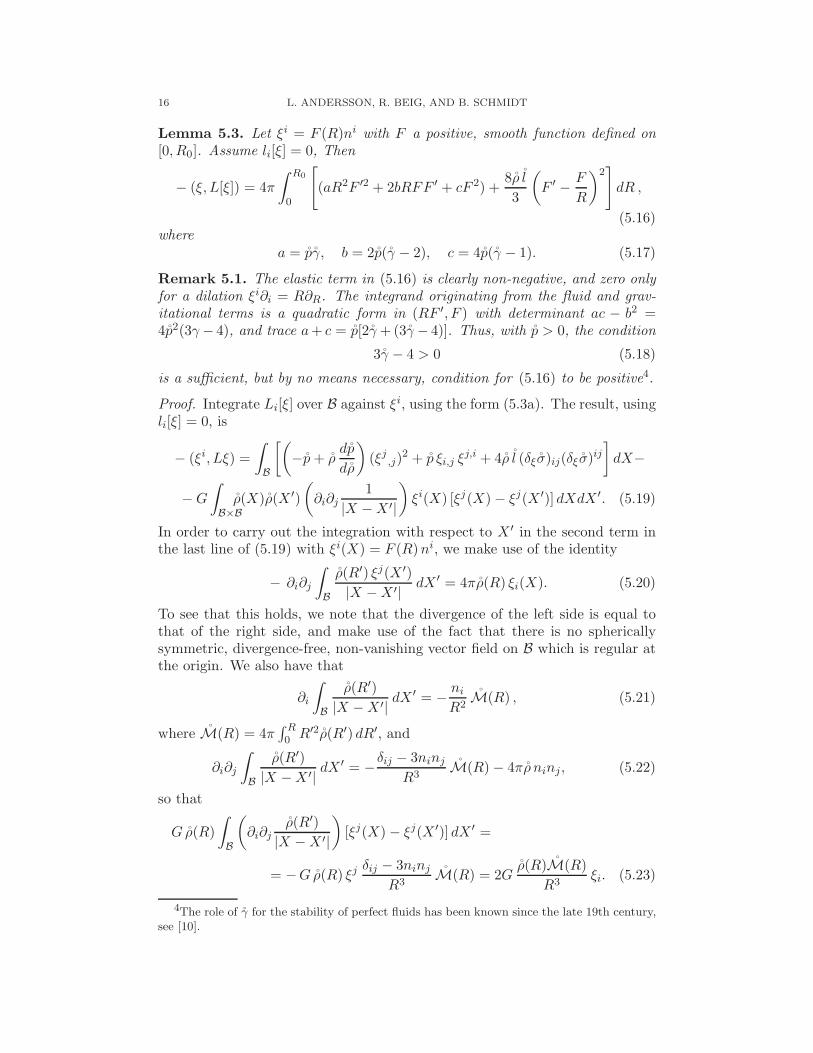
Lemma 5.3. Let ξi = F (R)ni with F a positive, smooth function defined on[0, R0]. Assume li[ξ] = 0, Then

− (ξ, L[ξ]) = 4π

∫ R0

0

[

(aR2F ′2 + 2bRFF ′ + cF 2) +8ρ l

3

(

F ′ − F

R

)2]

dR ,

(5.16)where

a = pγ, b = 2p(γ − 2), c = 4p(γ − 1). (5.17)

Remark 5.1. The elastic term in (5.16) is clearly non-negative, and zero onlyfor a dilation ξi∂i = R∂R. The integrand originating from the fluid and grav-itational terms is a quadratic form in (RF ′, F ) with determinant ac − b2 =4p2(3γ− 4), and trace a+ c = p[2γ+(3γ− 4)]. Thus, with p > 0, the condition

3γ − 4 > 0 (5.18)

is a sufficient, but by no means necessary, condition for (5.16) to be positive4.

Proof. Integrate Li[ξ] over B against ξi, using the form (5.3a). The result, usingli[ξ] = 0, is

− (ξi, Lξ) =

∫

B

[(

−p+ ρdp

dρ

)

(ξj ,j)2 + p ξi,j ξ

j,i + 4ρ l (δξσ)ij(δξ σ)ij

]

dX−

−G

∫

B×B

ρ(X)ρ(X ′)

(

∂i∂j1

|X −X ′|

)

ξi(X) [ξj(X)− ξj(X ′)] dXdX ′. (5.19)

In order to carry out the integration with respect to X ′ in the second term inthe last line of (5.19) with ξi(X) = F (R)ni, we make use of the identity

− ∂i∂j

∫

B

ρ(R′) ξj(X ′)

|X −X ′| dX ′ = 4πρ(R) ξi(X). (5.20)

To see that this holds, we note that the divergence of the left side is equal tothat of the right side, and make use of the fact that there is no sphericallysymmetric, divergence-free, non-vanishing vector field on B which is regular atthe origin. We also have that

∂i

∫

B

ρ(R′)

|X −X ′| dX′ = − ni

R2M(R) , (5.21)

where M(R) = 4π∫ R0 R′2ρ(R′) dR′, and

∂i∂j

∫

B

ρ(R′)

|X −X ′| dX′ = −δij − 3ninj

R3M(R)− 4πρ ninj, (5.22)

so that

G ρ(R)

∫

B

(

∂i∂jρ(R′)

|X −X ′|

)

[ξj(X)− ξj(X ′)] dX ′ =

= −G ρ(R) ξjδij − 3ninj

R3M(R) = 2G

ρ(R)M(R)

R3ξi. (5.23)

4The role of γ for the stability of perfect fluids has been known since the late 19th century,see [10].


Here we have used that the contribution of the last term in (5.22) cancelsthat from (5.20). Evaluating the first line in (5.19) is of course completelystraightforward. Thus for the non-elastic part of (5.19) we find the expression

4π

∫ R0

0R2

[

(

ρdp

dρ− p

)(

F ′ +2F

R

)2

+ p

(

F ′2 +2F 2

R2

)

− 2GρMF 2

R3

]

dR.

(5.24)But we know that

p′ = −G ρMR2

, (5.25)

cf. (3.17). Inserting (5.25) into (5.24) and integrating the last term by partsusing p (R0) = 0 gives the result.

Motivated by lemma 5.3 and the discussion in remark 5.1, we make thefollowing definition.

Definition 5.4. The reference body satisfies the radial stability condition if(5.18) holds, or more generally, if the quadratic form in (5.16) is positive defi-nite.

We now turn to the non-radial modes. These are analyzed using the form(5.5) and (5.6) for Li[ξ] respectively li[ξ], for a non-radial vector field ξi, underthe assumption li[ξ] = 0.

Define

δξµ =

(

dp

dρδξρ+ 4ρ l (δξσ)ij n

inj)∣

∣

∣

∣

∂B

, (5.26)

Then, cf. (5.3b), the condition li[ξ] = 0, implies

li[ξ]ni = ρ U ′ξini|∂B + δξµ = 0. (5.27)

Further, let U and u denote the Newtonian volume and single layer potentials,respectively, i.e.

U[f ] = −G

∫

B

f(X ′)

|X −X ′| dX′, (5.28)

and

u[f ] = −G∫

∂B

f(X ′)

|X −X ′| dS(X′). (5.29)

For convenience, we have not included the factor 1/4π here. Then we can write(see proposition 5.1)

δξU = U [δξ ρ]− u[ρ ξini] = U [δξρ] + u

[

δξµ

U ′

]

− u

[

li[ξ]ni

U ′

]

. (5.30)

The following proposition, which is proved starting from 5.5 by a straightfor-ward partial integration and making use of the above definitions, provides aformula for an expression which is essentially the second variation at the refer-ence deformation φ = id of the material form of the action given in equation(3.7).


Proposition 5.5. Let ξi be a vector field such that li[ξ] = 0. Then we have

− (ξ, L[ξ]) =

∫

B

1

ρ

dp

dρ(δξρ)(δξ ρ)dX +

∫

∂B

1

ρ U ′(δξµ)(δξµ)dS(X)+

+

∫

B

(δξ ρ)

(

U [δξρ] + u

[

δξµ

U ′

])

dX+

∫

∂B

1

U ′(δξµ)

(

U [δξρ] + u

[

δξµ

U ′

])

dS(X)+

+ 4

∫

B

ρ l (δξ σ)ij(δξ σ)ijdX. (5.31)

Remark 5.2. In addition to the elastic “bulk” contribution (third term in thefirst line in (5.31)), there are elastic contributions to all boundary terms in(5.31) resp. (5.29) via δξµ. In the absence of elasticity and when ρ(R0) =0, after insertion of (5.27), the expression (5.31) boils down to the famous“Chandrasekhar energy”, cf. [6, (5-49)]. Specializing to the radial case withli[ξ] = 0, the expression (5.31) of course coincides with (5.16). For this case itturns out to be simpler to derive (5.16) directly.

The following result is a generalization of the Antonov-Lebovitz theorem, cf.[6, §5.2] which allows for the the case where ρ(R0) > 0.

Proposition 5.6. Let ξi be a non-radial vector field such that li[ξ] = 0. Thenthe quadratic form −(ξ, Lξ) is non-negative, and zero if and only if ξi is aEuclidean Killing vector field.

Remark 5.3. Our proof of proposition 5.6 follows closely the proof valid underthe assumption ρ(R0) = 0 given in the book of Binney and Tremaine, cf. [6,Appendix 5.C]. The new edition, cf. [7, Appendix H] proves this result usinga more direct argument due to [1]. We have not been able to generalize thatargument to the case ρ(R0) > 0.

Proof. Note first of all that the last (purely elastic) term in (5.31) is non-negative and vanishes only on infinitesimal conformal motions. The remainingterms, on the other hand, depend only on pairs of functions, namely (δξρ, δξµ),on B × ∂B. Our claim amounts to the fact that, when restricted to pairs(δξ ρ, δξµ) with zero spherical mean, the sum of these terms is non-negative and

zero iff (δξ ρ, δξµ) = (ρ′(c, n),−ρ U ′(c, n)|∂B) for some constant vector c. To seethat we take pairs f = (δξ ρ, δξµ) to lie in the Hilbert space H defined by

H = L2

(

B, 1ρ

dp

dρdX

)

⊕ L2

(

∂B, 1

ρ U ′dS(X)

)

, (5.32)

with scalar product

〈f1|f2〉 =∫

B

1

ρ

dp

dρ(δ1ρ) (δ2ρ) dX +

∫

∂B

1

ρ U ′(δ1µ) (δ2µ) dS(X), (5.33)

and consider the operator V : H → H, defined by

V(δρ, δµ) =

(

ρdρ

dp

(

U [δξ ρ] + u

[

δξµ

U ′

])

, ρ

(

U [δξρ] + u

[

δξµ

U ′

]

|∂B))

. (5.34)

The operator V is self-adjoint with respect to the scalar product in (5.32), dueto the symmetry of the Poisson kernel.


By Lemma A.2, the volume potential U defines a continuous map L2(B) →H2(B). Further, the layer potential u defines a continuous map L2(∂B) →H1(∂B), cf. Lemma A.1. Since the scalar product (5.33) defines a norm on H

which is equivalent equivalent to the standard norm on L2(B) × L2(∂B), theoperator V : H → H is compact. Furthermore it maps (δρ, δµ)’s with vanishingspherical mean into themselves and its corresponding restriction is also self-adjoint and compact. Now the expression in (5.31) minus the elastic term takethe form

〈f |(E+ V)f〉. (5.35)

Since the operator V is compact and self-adjoint, it has a complete set of eigen-functions with real eigenvalues. We must show that for −λ in the spectrum ofV it holds that λ ≤ 1. Thus consider

λ δξρ+ ρdρ

dpδξU = 0, in B, (5.36)

and

λ δξµ+ (ρ δξU)|∂B = 0, in ∂B, (5.37)

where δξU = U [δξ ρ] + u

[

δξµ

U ′

]

. We write (5.36) in the form

∆δξU +4πG

λρdρ

dpδξU = 0. (5.38)

Furthermore we write δξU in the form

δξU = U ′δs = U ′∑

l

sl(R)Yl(Ω) , (5.39)

where we suppress the index m of spherical harmonics.Using the radial derivative of U ′′ + 2

R U′ = 4πGρ to eliminate U ′′′, it is

straightforward to show that (5.38) can be written in the form

1

R2U ′(R2U ′2s′l)

′ − l2 + l − 2

R2U ′sl − 4πG ρ

dρ

dpU ′

(

1− 1

λ

)

sl = 0. (5.40)

Integrating (5.40) over (0, R0) against R2U ′sl we find that

∫ r0

0R2U ′2

[

s′2l +

(

l2 + l − 2

r2+ 4πG ρ

dρ

dp

(

1− 1

λ

))

s2l

]

dR

−R20(U

′2sls′l)(R0) = 0. (5.41)

Next observe that the expression for δξU makes sense both in the interior and

exterior region, and that δξU is continuous across ∂B and δξU′ suffers a jump

[(δξU)′]∂B(r0) = 4πGδξµ

U ′(R0)= −4πG

λ

ρ δξU

U ′

∣

∣

∣

∣

∂B

= −4πG

λρ δs|B, (5.42)

where we have used (5.37) in the second equality. Since

[U ′′]|∂B = −4πGρ|∂B, (5.43)


it follows that

[δs′]∂B = 4πG

(

1− 1

λ

)(

ρ δs

U ′

)

∣

∣

∣

∂B(5.44)

This in turn implies that

[s′l](R0) = 4πG

(

1− 1

λ

)(

ρ sl

U ′

)

(R0). (5.45)

But, by virtue of the multipole expansion in the exterior region, we also havethat

limR↓R0

(

(U ′sl)′ +

l + 1

R0U ′sl

)

= 0 ⇒ limR↓R0

(

s′l +l − 1

R0sl

)

= 0 . (5.46)

Thus

limR↑R0

(

s′l +l − 1

R0sl

)

= 4πG

(

1

λ− 1

)(

ρ sl

U ′

)

(R0). (5.47)

Inserting (5.47) into (5.41), there results

∫ R0

0R2U ′2

[

s′2l +l2 + l − 2

R2s2l

]

dR+R0(l − 1)(U ′2 s2l )(R0) =

= 4πG

(

1

λ− 1

)[∫ R0

0ρdρ

dps2l dR+R2

0(U′ρ s2l )(R0)

]

. (5.48)

Thus (note that U ′ > 0 and, since δs has zero spherical mean, l ≥ 1) it followsthat λ ≤ 1 and λ = 1 implies that sl = 0 for l > 1 and s1 = const. This in turnmeans that δξU = U ′(c, n) = ci∂iU which implies

∆δξU = 4πG ρ′(c, n) . (5.49)

Thus δξρ = ρ′(c, n). It now follows that V restricted to quantities with zerospherical mean has eigenvalues λ ≤ 1 and λ = 1 implies that δξρ = ciρ,i.

Furthermore (5.37) now implies δξµ = −ρ U ′(c, n)|∂B .So far ξ itself was not involved in the argument. Going back to the definition(5.26) we infer that (δξ σijn

inj|∂B = 0. Now, due to the presence of the elasticterm in (5.31), it follows that (δξσ)ij = 0 everywhere in B, whence ξ is aconformal Killing vector. Dilations and conformal boosts are incompatible withδξρ = ciρ,i. The only remaining possibility is that ξi = ci + ΩijX

j with Ωij =Ω[ij].

Summing up we obtain the

Theorem 5.7. Assume that the radial stability condition, cf. definition 5.4,holds. Then the nullspace of Li, under the condition that li be zero consistsexactly of infinitesimal Euclidean motions.

As a final remark note that the Antonov-Lebovitz (i.e. non-radial-non-radial)part of the previous argument does not require any condition on the backgroundequation of state involving γ. It implies in particular that the kernel of the purefluid linearized operator acting on non-radial modes is trivial, i.e. only consistsof ξ’s being translations or satisfying δξρ = 0. This in turn implies that thereare no nontrivial nonspherical perturbations of a Newtonian perfect-fluid star


with given equation of state - which in turn is a linearized version of the classicalspherical-symmetry result of Lichtenstein.

6. Fredholm alternative

In this section we consider the operator

L : ξ → (−L[ξ], l[ξ]).We make use of the results and methods of [14, chapitre 2].

Let Lloc denote the local part of the operator L, corresponding to the first lineof (5.3a). Then ξ → L

locξ = (−Lloc[ξ], l[ξ]) is an elliptic, formally self-adjointdifferential operator of second order. Lloc is therefore Fredholm as a map

H2+k(B) → Hk(B)×H1/2+k(∂B),for k ≥ 0, k integer.

Further, let Z be the gravitational part of −L, given by the second line in(5.3a). Explicitely, for X ∈ B,

Zi[ξ](X) = Gξj(X)∂i∂jU(X)−−Gρ(X)

∫

B

(

∂i∂j1

|X −X ′|

)

ρ(X ′)ξj(X ′)dX

= Gξj(X)∂i∂jU + 4πGρ(X)∂i∂j(

∆−1(ρξjχB))

(X).

By assumption, the reference density ρ is smooth on B. By Lemma A.2, Z is abounded operator

Z : Hk(B) → Hk(B),for k ≥ 0, k integer. Hence, ξ 7→ (Z[ξ], 0) is a compact linear map

H2+k(B) → Hk(B)×H1/2+k(∂B),and hence it follows that L is Fredholm, since a compact perturbation of aFredholm operator is again Fredholm, cf. [11, Theorem 37.5]. In particular, Lhas finite dimensional kernel and closed range with finite dimensional cokernelgiven by kerL∗ where L

∗ is the operator mapping

H−k(B)×H−1/2−k(∂B) → H−2−k(B),defined by

〈Lξ,Φ〉 = 〈ξ,L∗Φ〉,where 〈·, ·〉 is the duality pairing. Explicitely, with Φ = (v, ϕ) we have

〈Lξ,Φ〉 =∫

B

−Li[ξ]bidx+

∫

∂Bli[ξ]τ

idS,

and rangeL is given by the space of F = (b, τ) such that∫

B

bividx+

∫

∂Bτiϕ

idS = 0,

for all Φ ∈ kerL∗. We have the Green’s identity∫

B

ηiLi[ξ]dx−∫

B

Li[η]ξidx =

∫

∂Bηili[ξ]dS(x)−

∫

∂Bli[η]ξ

idS.

Now consider the case k = 0. Since Φ ∈ kerL∗ is equivalent to

〈ξ,L∗Φ〉 = 〈Lξ,Φ〉 = 0,


for all ξ ∈ H2(B), we have for Φ = (v, ϕ) ∈ kerL∗,

0 =

∫

B

−Li[ξ]vidx+

∫

∂Bli[ξ]ϕ

idS

=

∫

B

−ξiLi[v]dx +

∫

∂Bξili[v] +

∫

∂B(ϕi − vi)li[ξ]dS.

Since ξ ∈ H2(B) is arbitrary, this gives immediately that Li[v] = 0. Further,we have that (ξ, l[ξ]) is a Dirichlet system on ∂B, and hence it follows thatli[v] = 0 and ϕi = vi on ∂B. It follows from the analysis in [14] that the kerneland cokernel of L are independent of k, and hence are well-defined. We end upwith the following result.

Proposition 6.1. Assume that the radial stability condition, cf. definition 5.4,holds. Let k ≥ 0, k integer. The operator ξ 7→ L[ξ] = (−L[ξ], l[ξ]) is a Fredholmoperator

H2+k(B) → Hk(B)×H1/2+k(∂B),with finite dimensional kernel, and range consisting of (bi, τi) such that

∫

B

−bividx+

∫

∂Bτiv

idS = 0,

for all v ∈ kerL.

7. Implicit function theorem

In this section, we assume that the radial stability condition, cf. definition5.4, holds. Let ρλ, λ ∈ (−ǫ, ǫ) be a 1-parameter family of densities on B. LetF [ρλ, φ] = (bi[ρλ, φ], τi[ρλ, φ]) where

bi[ρ, φ] = −∂A(ρτAi) + ρ(∂iU) φ,τi[ρ, φ] = τAinA

∣

∣

∂B.

The Frechet derivative of F at the reference state λ = 0, φ = id is

DφF∣

∣

λ=0,φ=idξ = L ξ = (−L[ξ], l[ξ]).

By theorem 5.7, and proposition 6.1 we have that the kernel and cokernel ofDΦF consists of Killing vector fields, i.e. ζ i of the form ci+ωijX

j for constantci, ωij, ωij = ω[ij].

Now let P be the projection defined by P : (bi, τi) 7→ (b′i, τi), with

b′i = bi + ci + ωijXj ,

for suitable ci, ωij such that (b′i, τ i) are equilibrated, i.e.∫

B

b′iζidx−

∫

∂Bτiζ

idS = 0,

for all ζ i ∈ kerL. The above determines b′i in terms of bi and τi and hence alsothe projection operator P.

We eliminate the kernel of L = DφF∣

∣

λ=0,φ=idby fixing the 1-jet of φ at the

origin. Denote the space of ξi ∈ H2+k(B) with ξi(0) = 0, ∂iξj(0) = 0 by X andlet Y denote the range of L. Then we have that L : X → Y is an isomorphism.


Now the following result is an immediate consequence of the implicit functiontheorem.

Proposition 7.1. Fix k ≥ 1 and ǫ > 0. For λ ∈ (−ǫ, ǫ), let λ 7→ ρλ be a1-parameter family of smooth functions on B, so that ρ = ρ0 is a solution toF [ρ, id] = 0. There is an ǫ0 > 0 so that for λ ∈ (−ǫ0, ǫ0), there is a uniqueφλ ∈ H2+k(B) with φ(0) = 0, ∂jφ

i(0) = δij , such that

PF [ρλ, φλ] = 0.

7.1. Equilibration. Recall that the the field equation in the Eulerian picturetakes the form

∇i(τijχf−1(B) +Θi

j) = 0.

For ζ i a Killing field we have ∇(iζj) = 0 and hence

∫

R3

ζj∇i(τijχf−1(B) +Θij)dx = −

∫

R3

∇iζj(τijχf−1(B) +Θij)dx = 0,

since τ ij = τ (ij) and Θij = Θ(ij). Recall

∇iΘij = ρχf−1(B)∂jU.

Applying the change of variables formula and the Piola identity, and takinginto account the boundary condition τ ijni

∣

∣

∂f−1(B)= 0 we have

0 =

∫

B

ζj φ[−∂AτAj + (∂jU) φ]dX,

and hence (bi, 0) is equilibrated with respect to ζ i φ.We are now ready to prove

Theorem 7.2. Assume that the radial stability condition holds. Fix k ≥ 1and ǫ > 0. For λ ∈ (−ǫ, ǫ), let λ 7→ ρλ be a 1-parameter family of smoothfunctions on B, so that ρ = ρ0 is a solution to F [ρ, id] = 0, and ρλ

∣

∣

∂B= ρ0

for λ ∈ (−ǫ, ǫ). There is an ǫ0 > 0 so that for λ ∈ (−ǫ0, ǫ0), there is a uniqueφλ ∈ H2+k(B) with φ(0) = 0, ∂jφ

i(0) = δij , such that

F [ρλ, φλ] = 0.

Proof. Let φλ be the solution to PF [ρλ, φλ] = 0 constructed in proposition 7.1,and let K denote the space of Killing fields on R

3. By the proof of proposition7.1 we have that the load bi = bi[ρλ, φλ] corresponding to φλ satisfies bi ∈ K.On the other hand, we have by the above discussion that

∫

B

ζ i φλbi = 0, ∀ζ i ∈ K.

For φλ sufficiently close to id this implies bi = 0. Since φλ depends continuouslyon λ, the result follows.


8. Non-spherical nature of solutions

It is important to understand that the method we have developed in thiswork is capable of “building mountains”, i.e. that the solutions we constructare indeed non-spherical. Before proving that this is the case, it will be useful tomake a few observations on the pure fluid case, where the action in the materialframe (3.7) takes the (static Euler-Poisson) form

Lep[ρ;φ] =∫

B

ρ(X) e(ρ det(φjB)−1)(X)dX

− G

2

∫

B×B

ρ(X)ρ(X ′)dX dX ′

|φ(X) − φ(X ′)| . (8.1)

Let ψ be a diffeomorphism ψ : B → B (in particular ψ maps ∂B into itself).

Further, let ρψ = ρ ψ | ∂ψ∂X |, where | ∂ψ∂X | = det(ψiA), and φψ = φ ψ. Then theaction given by (8.1) satisfies the covariance property

Lep[ρ ;φ] = Lep[ρψ;φψ]. (8.2)

This covariance property is of course reflected by the fact that the Eulerianvariable ρ[ρ, φ](x) = (ρ | ∂φ∂X |−1)(φ−1(x)) remains unchanged under the action of

ψ on (ρ, φ). It follows that the Euler-Poisson system is symmetric5 under theaction of the infinite dimensional group of volume preserving diffeomorphismsψ of B, i.e. when ψ leaves the volume form ρ dX invariant, then

Lep[ρ;φ ψ] = Lep[ρ;φ].Next recall from a theorem of Moser [16] that for any positive densities ρ1, ρ2in B such that

∫

Bρ1dX =

∫

Bρ2dX there exists a diffeomorphism ψ : B → B,

such that ρ2 = ρ1 ψ | ∂ψ∂X |. Thus, for fluids, any change of density ρ leaving itsintegral over B unchanged, should be viewed as a mere change of gauge. Notethat

∫

Bρ dX is nothing but the total mass of the physical solution, namely

∫

φ(B) ρ[ρ, φ](x) dx.

Remark 8.1. The above transformation properties explain the fact that thelinearized operator (5.3), in the absence of the elastic terms, has a kernel con-taining translations plus the infinite dimensional set of vector fields ξ satisfyingδξρ = 0 and ξini|B = 0. When the radial stability condition, cf. definition 5.4,

holds, the proofs of lemma 5.3, and of proposition 5.6 in the case where l is zero,show that the kernel in fact consists of these vector fields. Finally, we remarkthat the transformation properties can be used to derive the identity stated inproposition 5.1. The proof of the last statement is left to the reader.

Let δρ = ddλ ρλ|λ=0. Before stating our proposition on lack of spherical sym-

metry we prove two lemmas. The first concerns the form of the perturbedEulerian density and Cauchy stress.

5Not that covariance refers to a change of both the field variable φ and the backgroundfield, whereas symmetry refers to change of field variable leaving the background invariant.For example, special relativistic Maxwell theory (the background field in this case beingthe Minkowski metric) is covariant under spacetime diffeomorphisms but symmetric underPoincare transformations.


Lemma 8.1. There holds

d

dλρ[ρλ, φλ]

∣

∣

∣

∣

λ=0

= δρ− δξρ, (8.3)

andd

dλτij [ρλ, φλ]

∣

∣

∣

∣

λ=0

=dp

dρ(δρ− δξρ)δij − 4ρ l (δξ σ)ij . (8.4)

Proof. The proof of (8.3) follows easily from (3.13). The proof of (8.4) followsfrom (5.2) together with (3.9).

The second lemma concerns the linearized problem.

Lemma 8.2. The linearized problem, namely

DφF [ρ, id].ξ = −Dρ F [ρ, id].δρ (8.5)

takes the explicit form

ρ ∂i

(

1

ρ

dp

dρδξρ+ δξU

)

+ 4 ∂j[

ρ l (δξ σ)ij

]

= ρ ∂i

(

1

ρ

dp

dρδρ

)

−Gρ ∂i

∫

B

(δρ)(X ′)

|X −X ′|dX′, (8.6a)

for the bulk and[(

dp

dρδξρ+ ρ U ′ξjnj

)

ni + 4ρ l (δξσ)ijnj

] ∣

∣

∣

∣

∂B

=

(

dp

dρδρ

)

ni

∣

∣

∣

∣

∂B

, (8.6b)

for the boundary part.

Proof. The left hand side of (8.5) is clearly given by (5.5). To deal with theright hand side, we first note that since the invariant τ is independent of ρ, theelastic contribution to the right hand side of (8.6a) is zero. Now the form ofthe right hand side of equation (8.6a) follows by explicit computation from thefluid Euler-Lagrange equation, namely

E [ρ, φ]i = −∂A∂ [ρ e(ρ det(φjB)

−1)]

∂φiA

−Gρ(X)

∫

B

(

∂i1

|z|

)∣

∣

∣

∣

z=φ(X)−φ(X′)

ρ(X ′)dX ′, (8.7)

in B. Finally, the form of the right hand side in the boundary condition (8.6b)follows easily from

Dρ τAi[ρ, id] = −dp

dρδAi, (8.8)

which in turn follows from (5.1).

We now state our result on lack of spherical symmetry.

Proposition 8.3. Suppose l > 0. and that the stability condition (5.18) issatisfied. Let a non-zero function δρ on B be given, which has only l ≥ 2nonzero modes6 in its spherical harmonics expansion, and which has δρ|∂B = 0.

6The index l should not be confused with l(ρ, τ, δ) or l.


Then the perturbed stress of the physical body, given by (8.4), is not spher-ically symmetric. Here the perturbed stress is calculated with respect to theunique vector field ξi solving equation (8.5), constructed as in section 7.

Remark 8.2. The proof of proposition 8.3 applies more generally in the casewhen the quadratic form, defined by (5.16) with the elastic terms set to zero, ispositive definite.

Proof. We first show that with the given δρ, the right hand side of (8.6a), whichwe shall denote by Hi, is non-zero. Assume for a contradiction, that Hi is zero.

Since δρ has only l ≥ 2 modes, it holds that∫

B

δρ dX = 0

and hence there is a vector field ηi such that δηρ = δρ and ηini|∂B = 0.Inserting δηρ into the right hand side of equation (8.6a), and taking into

account that δρ|δB = 0, we see that Hi is identical to Li[η] given by (5.5) for

the particular case when the elastic term is absent, i.e., with l = 0.It follows from δρ|∂B = 0 that the vector field ηi satisfies ∂iη

i|∂B = 0. Hencewe have that η is in the null space of the operator Li given by (5.5) and satisfies

the boundary condition (5.27), both in the case l = 0. Then the proof of

proposition 5.6 in the case where l = 0 shows that either η is a translationKilling vector or δηρ = 0. If δηρ we have a contradition, and hence η is atranslation. However, in this case, δρ has only l = 1 components, and it followsthat δρ = 0, which gives a contradition. Thus we have proved that Hi isnon-zero.

Further, by construction, Hi has only l ≥ 2 components. To make concretewhat this means for a (co-)vector field, recall that any covector κi can be writtenin the form

κi = ani + (δij − nin

j)∂jb+ ǫijknj∂kc

where a, b, c are scalar fields on [0, R0] × S2 with a unique, and b, c unique up

to constants. The triple of scalars (a, b, c) corresponding to covector Hi hasnon-zero l ≥ 2 components in its spherical harmonics expansion. Due to thestability condition (5.18), the boundary value problem given (8.6) has a solutionξi, which is unique up to Killing vectors.

Recall that Killing vectors have only l ≥ 1 components. It follows that wecan set the l ≤ 1 components of ξi to zero, and get a solution which we alsodenote ξi to (8.6), such that ξi has only l ≥ 2 components.

Finally we show that the the perturbed Eulerian stress tensor (8.4) is notspherically symmetric. To do this we note that if it were spherically symmetric,then its tracefree part would be of the form

− 4ρ l (δξ σ)ij = A(δij − 3ninj) (8.9)

for some function A depending only on R. Since by construction ξi is non-zeroand has only l ≥ 2 modes, equation (8.9) can have a solution only if A = 0and ξi is a conformal Killing vector. But conformal Killing vectors have onlyl ≤ 1 modes, which is a contradiction. Therefore, the perturbed Eulerian stressis not spherically symmetric, which completes the proof.


We finally point out that it would be interesting to have information aboutthe spherical behavior of ξini|∂B, since this describes the shape of mountains toorder λ. However, this would require a detailed analysis of the boundary valueproblem given by (8.6), which we defer to later work.

Acknowledgements. This material is based in part on work supported by theNational Science Foundation under Grant No. 0932078 000, while LA and RBwere in residence at the Mathematical Sciences Research Institute in Berkeley,California, during the semester programme of Mathematical General Relativ-ity, during the fall of 2013. Further, LA and RB thank ESI for hospitalityand support during part of this work. BS is grateful to Jorg Frauendiener fordiscussions in the early stages of the present work.

Appendix A. Estimates for the Newtonian potential

Here we prove some potential theoretic estimates which are used in our anal-ysis. We discuss here only estimates in the setting of L2 Sobolev spaces Hs.See [20, Chapter 4] for background. The analogous results hold in the settingof Sobolev spaces of Lp type W s,p.

Consider Rn, n ≥ 3, with Cartesian coordinates (xi), and with the Euclideanmetric. Let Ω be a smooth, bounded domain in R

n, with boundary ∂Ω. Letni be the outward directed normal to ∂Ω. The trace of a function f on ∂Ω isdenoted Tr∂Ω f .

Let ωn be the area of the unit sphere in Rn, and let E = −1/(ωn|x|n−2) be

the fundamental solution of the Laplace equation. The volume potential of afunction f is

V[f ](x) =∫

ΩE(x− x′)f(x′)dx′,

and the layer potential S[f ] is

S[f ](x) =∫

∂ΩE(x− x′)f(x′)dS(x′),

where dS is the induced volume element on ∂Ω. We shall need the followingstandard result, cf. [19, Chapter 7, Proposition 11.2]. (See also [19, Chapter 7,Proposition 11.5] The assumption that the complement of Ω is connected madein [19, Chapter 7, Proposition 11.5] is not relevant for the continuity propertywhich we need here.)

Lemma A.1. S defines a bounded operator S : Hs−1(∂Ω) → Hs(∂Ω).

Let χΩ denote the indicator function of Ω, i.e.

χΩ(x) =

1 x ∈ Ω,0 x /∈ Ω,

and let δ∂Ω be the delta-distribution supported on ∂Ω. Let f be sufficientlyregular so that the trace Tr∂Ω f is defined. Then the following identity is validin the sense of distributions.

∂i(fχΩ) = (∂if)χΩ − Tr[fni]δ∂Ω. (A.1)


To see this, let φ ∈ C∞0 (Rn) and let ξi be a vector field on R

n. Then we have∫

Rn

φξi∂iχΩdx =

∫

Rn

φ∂i(ξiχΩ)− φ(∂iξ

i)χΩdx

= −∫

Rn

∂iφξiχΩ − φ(∂iξ

i)χΩdx

= −∫

∂Ω

φnidS −∫

Rn

φ(∂iξi)χΩdx.

Specializing to the case ξk∂k = ∂i gives (A.1). From (A.1) we have immediately,by the chain rule and the differentiation formula for convolutions,

∂iV[f ] = V[∂if ]− S[fni]. (A.2)

We can now prove the following.

Lemma A.2. Let s ≥ 0, s integer. Then V defines a continuous map

V : Hs(Ω) → Hs+2(Ω).

Proof. The case s = 0 follows from the standard interior estimate for thePoisson equation, cf. [14, Chapitre 2, Theoreme 3.1]. The proof now pro-ceeds by induction, with s = 0 as base. Let s ≥ 1 and suppose we haveproved the statement for s − 1. Let f ∈ Hs(Ω). By the trace theorem,[20, Chapter 4, Proposition 4.5], Tr∂Ω[fn

i] ∈ Hs−1/2(∂Ω) and by lemma A.1,

S[fni] ∈ Hs+1/2(∂Ω). Now, S[fni] is harmonic in Ω with trace on ∂Ω in

Hs+1/2. It follows that S[fni] ∈ Hs+1(Ω). Further, by the induction hypoth-esis, V[∂if ] ∈ Hs+1(Ω), and hence ∂iV[f ] ∈ Hs+1(Ω). Again by the inductionhypothesis, V[f ] ∈ Hs+1(Ω), and hence it follows that V[f ] ∈ Hs+2(Ω), whichcloses the induction and gives the result.

References

[1] Jean-Jacques Aly and Jerome Perez, On the stability of a gaseous sphere against non-

radial perturbations, Monthly Notices Roy. Astronom. Soc. 259 (1992), no. 1, 95–103.MR 1187889 (93i:85002)

[2] L. Andersson, T. A. Oliynyk, and B. G. Schmidt, Dynamical elastic bodies in Newtonian

gravity, Classical and Quantum Gravity 28 (2011), no. 23, 235006.[3] Lars Andersson, Robert Beig, and Bernd Schmidt, Static self-gravitating elastic bodies in

einstein gravity, Communications on Pure and Applied Mathematics 61 (2008), no. 7,988–1023.

[4] R. Beig and B. G. Schmidt, Relativistic elasticity, Classical and Quantum Gravity 20

(2003), 889–904.[5] Robert Beig and Bernd G. Schmidt, Static, Self-Gravitating Elastic Bodies, Proc. Roy.

Soc. Lond. A459 (2003), 109–115.[6] James Binney and Scott Tremaine, Galactic dynamics, Princeton series in astrophysics,

Princeton Univ. Press, Princeton, NJ, 1987.[7] , Galactic dynamics, Princeton series in astrophysics, Princeton Univ. Press,

Princeton, NJ, 2008.[8] S. Calogero and T. Leonori, Ground states of self-gravitating elastic bodies, ArXiv e-prints

(2012).[9] Nicolas Chamel and Pawel Haensel, Physics of neutron star crusts, Living Reviews in

Relativity 11 (2008), no. 10.


[10] S. Chandrasekhar, An introduction to the study of stellar structure, Dover PublicationsInc., New York, N. Y., 1957.

[11] John B. Conway, A course in operator theory, Graduate Studies in Mathematics, vol. 21,American Mathematical Society, Providence, RI, 2000.

[12] Jerzy Kijowski and Giulio Magli, Unconstrained variational principle and canonical struc-

ture for relativistic elasticity, Rep. Math. Phys. 39 (1997), no. 1, 99–112.[13] Leon Lichtenstein, Gleichgewichtsfiguren rotierender flussigkeiten, Springer, Berlin, 1933.[14] J.-L. Lions and E. Magenes, Problemes aux limites non homogenes et applications. Vol.

1, Travaux et Recherches Mathematiques, No. 17, Dunod, Paris, 1968.[15] Jerrold E. Marsden and Thomas J. R. Hughes, Mathematical foundations of elasticity,

Dover Publications Inc., New York, 1994, Corrected reprint of the 1983 original.[16] Jurgen Moser, On the volume elements on a manifold, Trans. Amer. Math. Soc. 120

(1965), 286–294.[17] A. D. Rendall and B. G. Schmidt, Existence and properties of spherically symmetric static

fluid bodies with a given equation of state, Classical and Quantum Gravity 8 (1991), 985–1000.

[18] A. Shadi Tahvildar-Zadeh, Relativistic and nonrelativistic elastodynamics with small shear

strains, Ann. Inst. H. Poincare Phys. Theor. 69 (1998), no. 3, 275–307.[19] Michael E. Taylor, Partial differential equations. II, Applied Mathematical Sciences, vol.

116, Springer-Verlag, New York, 1996, Qualitative studies of linear equations.[20] , Partial differential equations I. Basic theory, second ed., Applied Mathematical

Sciences, vol. 115, Springer, New York, 2011.

E-mail address: [email protected]

Albert Einstein Institute, Am Muhlenberg 1, D-14476 Potsdam, Germany


Gravitational Physics, Faculty of Physics, University of Vienna,

Boltzmanngasse 5, A-1090 Vienna, Austria


Max-Planck-Institut fur Gravitationsphysik, Albert-Einstein-Institut,

Am Muhlenberg 1, D-14476 Golm, Germany

ELASTIC DEFORMATIONS OF COMPACT...

Documents

Transcript of ELASTIC DEFORMATIONS OF COMPACT...