CIRPÉE Centre interuniversitaire sur le risque, les politiques économiques et l’emploi Cahier de recherche/Working Paper 05-32 Default Risk in Corporate Yield Spreads Georges Dionne Geneviève Gauthier Khemais Hammami Mathieu Maurice Jean-Guy Simonato Novembre/November 2005 _______________________ Dionne, Gauthier, Hammami, Maurice, Simonato: HEC Montréal Dionne: Corresponding author: georges.dionne@hec.ca The authors acknowledge the financial support of the National Science and Engineering Research Council of Canada (NSERC), of the Fonds québécois de recherche sur la nature et les technologies (FQRNT), of the Social Sciences and Humanities Research Council of Canada (SSHRC), of the Institut de Finance Mathématique de Montréal (IFM2), and of the Centre for Research on E-finance (CREF). Previous versions of the paper were presented at the Second International Conference on Credit Risk (Montreal, April 2004), at the SCSE annual conference (Quebec, 2004), at the C.R.E.D.I.T. Risk Conference (Venesia, 2004), and at the finance department of the University of Toronto (2005).

Abstract: An important research question examined in the recent credit risk literature focuses on the proportion of corporate yield spreads which can be attributed to default risk. Past studies have verified that only a small fraction of the spreads can be explained by default risk. In this paper, we reexamine this topic in the light of the different issues associated with the computation of transition and default probabilities obtained with historical rating transition data. One significant finding of our research is that the estimated default-risk proportion of corporate yield spreads is highly sensitive to the term structure of the default probabilities estimated for each rating class. Moreover, this proportion can become a large fraction of the yield spread when sensitivity analyses are made with respect to recovery rates, default cycles in the economy, and information considered in the historical rating transition data. Keywords: Credit risk, default risk, corporate yield spread, transition matrix, default probability, Moody's, Standard and Poor's, recovery rate, data filtration, default cycle. JEL Classification: G11, G12, G13, G21, G23 Résumé: Une importante question de recherche dans la littérature récente sur le risque de crédit aborde la proportion de l’écart de rendement entre les obligations privées et publiques (prime de crédit) pouvant être attribuée au risque de défaut. Des études antérieures ont démontré que cette proportion est faible (maximum 25 %). Dans cette recherche, nous réexaminons cette question en considérant différentes problématiques associées au calcul des probabilités de transition et de défaut obtenues des données historiques des transitions de notation de crédit. Un résultat important de notre recherche est que la proportion attribuable au risque de défaut dans les primes de crédit est sensible à la structure par terme des probabilités de défaut de chaque classe de risque. De plus, cette proportion peut devenir importante lorsque des analyses de sensibilité sont réalisées en fonction des taux de recouvrement, des cycles de défaut et de l’information considérée dans les données historiques des transitions de notation de crédit. Mots clés: Risque de crédit, risque de défaut, prime de crédit, matrice de transition, probabilité de défaut, Moody’s, Standard and Poor’s, taux de recouvrement, filtre de données, cycle de défaut.

1 Introduction

An important research question studied in the recent credit risk literature examines the proportion of corpo-

rate yield spreads explained by default risk. This question is not only important for the pricing of bonds and

credit derivatives but also for computing banks’ optimal economic capital for credit risk (Crouhy, Galai, and

Mark, 2000; Gordy, 2000). For example, in CreditMetrics (1997), all corporate yield spreads are assumed to

be explained by default risk, so the implied capital charge for default risk can be too high if other factors

enter in the composition of the spreads.

Elton, Gruber, Agrawal and Mann (Elton et al., 2001) have verified that only a small fraction of corporate

yield spreads can be attributed to default risk or expected default loss. They got their result from a reduced

form model and have shown that the expected default loss explains no more than 25% of corporate spot

spreads. The remainder is attributed to a tax premium and a risk premium for systematic risk. More

recently, Huang and Huang (2003) reached a similar conclusion with a structural model. They verified that,

for investment-grade bonds (Baa and higher ratings), only 20% of the spread is explained by default risk.

One of the key inputs needed for such assessments is an estimate of the term structure of default proba-

bility, that is, the probability of defaulting for different time horizons. To get these quantities, databases on

historical default frequencies from Moody’s and Standard and Poor’s can be used. For example, one can first

come up with an estimate of transition probabilities between rating classes and then use them to compute

the term structure of the default probability. This is the approach used in Elton et al. (2001). Although

this method appears straightforward, obtaining probability estimates with such a procedure is not a trivial

exercise. Many important issues arise in the process and the different choices made by the analyst might

lead to different results.

A first choice to make when computing default and transition probabilities is the period over which the

estimation is to be performed. As shown in Bangia et al. (2002), transition-matrix estimates are sensitive

to the period in which they are computed. Business and credit cycles might have a serious impact on the

estimated transition matrices and might lead to highly different estimates for the default-risk proportion.

A second issue calling for close attention concerns the statistical approach (Altman, 1998). Because

defaults and rating transitions are rare events, the typical cohort approach used by Moody’s and Standard

and Poor’s will produce transition probabilities matrices with many cells equal to zero. This does not mean

that the probability of the cell is nil but that its estimate is nil. Such a characteristic could lead economic

agents to underestimate the default-risk fraction in corporate yield spreads. Lando and Skodeberg (2002)

have shown that a continuous-time analysis of rating transitions using generator matrices improves the

estimates of rare transitions even when they are not observed in the data, a result that cannot be obtained

with the discrete-time cohort approach of Carty and Fons (1993) and Carty (1997).

Finally, a third important issue arising in the computation of default and transition probabilities is the

data filtering process which determines the information considered about issuers’ movements in the database.

For example, we must decide whether or not to consider issuers that are present at the beginning of the

estimation period but leave for reasons other than default (withdrawn rating or right censoring). Another

choice is whether or not to consider issuers that enter the database after the starting date of estimation.

2

Again, these choices might have non-negligible impacts on the final estimates.

In this article, we revisit the topic of corporate rate spread decomposition in light of the above consid-

erations. In a first step, we introduce a simple discrete-time model for estimating the proportion of the

corporate rate spread attributable to default risk. This model is then implemented using estimates of tran-

sition probabilities from the cohort method and computed for different periods of the default cycle. The

results show that matching the periods over which the probabilities are computed with the period over which

the spreads are examined can raise the proportion of the corporate yield spreads attributable to default risk.

For example, for A rated bonds, this proportion jumps from 9% to 23% (Table 3b, panel B, 1987-1991). For

Baa bonds, this proportion jumps from 32% to 65% (Table 3b, panel C, 1987-1991). As we shall see in more

detail, the 1987-1991 sub-period corresponds to a high default cycle in the bond market. The above results

are confirmed by a the continuous-time analysis of transition ratings in line with Lando and Skodeberg (2002)

(Table 3b, MDC columns). The analysis also highlights the importance of using the proper recovery rates

when estimating the proportion of the yield spread attributed to default risk. For Baa bonds, for example,

the above proportion of 65% corresponds to a recovery rate of 49%. This proportion jumps to 74% when

the recovery rate is cut to 40%, a more plausible rate in a high default risk period (Table 5).

In a second step, we look to see how sensitive our results are to the modelling approach taken and to

the information considered in the database. For this purpose, we introduce an alternative continuous-time

model. We also use this model to compute the approximate confidence intervals, in the spirit of Christensen,

Hansen, and Lando (2004). Three data filtering processes for different types of information are examined

: the first includes issuers that enter after the starting date of estimation (entry firms hereafter) as well

as withdrawn-rating observations; the second one excludes entry firm observations; and the third excludes

both entry firms observations and withdrawn-rating observations. Our results –when excluding withdrawn-

rating and entry firm observations– show that the average spread proportion attributed to default risk

for a maturity of ten years climbs to 71% for Baa rated bonds during the 1987-1991 period, with a 95%

approximate interval of 56% and 86% when the recovery rate is 49% (Table 8b).

The rest of the paper is organized as follows. In Section 2, we describe how the empirical bond-spread

curves are estimated. In Section 3, we present the discrete-time model used to estimate the default proportion

of the corporate yield spread for different rating categories and maturities. This section also presents the

results on the default-risk proportion obtained with this model and examines their sensitivity to assumptions

about default cycles, estimation methodology of probabilities and recovery rates. The sensitivity of our

modelling approach is then examined in Section 4 with the use of a continuous-time model. This section also

presents results including inference obtained by Monte Carlo simulations and a detailed sensitivity analysis

about the information considered in the databases. Section 5 concludes.

3

2 Empirical Bond-Spread Curves

2.1 Database Description

The data come from the Lehman Brothers Fixed Income Database (Warga, 1998). We choose this data to

enable comparisons with other articles in this literature using the same database. Moreover, the database

covers two default cycles an issue that will become important in the analysis. The data contains information

on monthly prices (quote and matrix), accrued interest, coupons, ratings, callability and returns on all

investment-grade corporate and government bonds for the period from January 1987 to December 1996. All

bonds with matrix prices and options were eliminated; bonds not included in Lehman Brothers’ bond indexes

and bonds with an odd frequency of coupon payments were also dropped.1 Appendix A.1, provides details

on the treatment of accrued interest.

As in Elton et al. (2001), month-end estimates of the yield-spread curves on zero-coupon bonds for each

rating class are needed to implement the models. These yield-spread curves are obtained by first estimating

the parameters associated with the Nelson and Siegel curve fitting approach. Appendix A.2 provides a brief

summary of this approach. All bonds with a pricing error higher than $5 are dropped. We then repeat

this estimation and data removal procedure until all bonds with a pricing error larger than $5 have been

eliminated. Using this procedure, 776 bonds were eliminated (one Aa, 90 A and 695 Baa) out of a total of

33,401 bonds found in the industrial sector, which is the focus of this study.

2.2 Empirical Analysis of Bond-Spread Curves

For each of the 120 months of this study, we first estimate the forward rate curve associated with government

bonds.2 The industrial corporate bonds are then grouped in three categories: Aa, A, and Baa. For each

category, we estimate the corporate forward rate curves. Our results are coherent, in that all of our estimated

empirical bond-spread curves are positive. Moreover, the bond-spread curves between a high rating class

and a lower rating class are also positive. Throughout this article, we shall use the expression “spot rate”

to indicate the yield to maturity on a zero-coupon bond. Figure 1 shows the empirical spreads on industrial

bonds of six years maturity for the ratings Aa, A, and Baa. We observe that the spreads are higher during

the January 1987-December 1991 sub-period.

(Figure 1 here)

Table 1 reports our results for corporate yield spreads for two to ten years of maturity. The results

are very close to those presented in Table 1 of Elton et al. (2001) for the industrial sector. The small

discrepancies might be explained by differences in data sets and estimation algorithms. In panel A, the

results cover the entire 10-year period, while in panels B and C they refer to two sub-periods of five years. It

1We did, however, keep three categories from the list of eliminations in Elton et al.(2001), because we lacked the informationneeded to identify them: government flower bonds, inflation-indexed government bonds, and bonds with floating rate debt. Aswe shall see, this makes no difference in the results.

2Recent studies (see, for example, Hull et al. 2005) argued that the Treasury rate is not the appropriate risk-free-rate. Weshall return to this issue in Section 4.3.

4

is important to observe that the average spreads are higher in the 1987-1991 sub-period than in the 1992-1996

sub-period. This difference will matter in the next sections where we explain the proportions of the corporate

yield spreads associated with default risk. The two sub-periods represent two different default cycles. The

1987-1991 sub-period is usually associated with a high default cycle while the sub-period 1992-1996 tends

to coincide with a low default cycle. The 1987-1991 period contains a macroeconomic recession and the US

loan crisis.

Figure 2 presents default rates extracted from Moody’s database (Moody’s, 2005). We observe that the

distribution of these rates over time has a shape similar to that of the empirical spreads for six years maturity

in Figure 1. This suggests that the link between the default-risk proportion and the default risk should vary

with the default cycles (see also Manning, 2004, for a similar conclusion).

(Figure 2 here)

Another interesting graph shown in Figure 3 examines how the average recovery rate varies with time.

These recovery rates were obtained from Moody’s database (Moody’s, 2005) and are defined as the ratio

of the defaulted bond’s market price, observed 30-days after its default date, to its face value (par). The

average recovery rates vary significantly with the default cycles defined above. For example, the average

recovery rate for all bonds during the 1987-1991 sub-period is equal to 40.8% while that of the 1992-1996

sub-period is equal to 45.5%. Those for senior unsecured bonds vary between 45.5% and 50.66% for the same

sub-periods. It is also documented in Moody’s (2005) that the recovery rates are even lower for industrial

bonds. Altman et al. (2003) present an interesting review of the literature on the link between recovery rate

and default probability.

(Figure 3 here)

Table 2 compares the average squared-root mean errors of the difference between theoretical bond prices

computed using the Nielson-Siegel model and the actual bond prices for treasuries and industrial corporate

bonds. Again our results are similar to those of Elton et al. (2001).

3 Discrete-Time Model

3.1 Model

The corporate yield spread is defined as the difference between the yield curves of the risky zero-coupon

bond and the risk-free, zero-coupon bond. Therefore, to characterize corporate yield spreads, one need only

model the values of a risk-free and a corporate zero-coupon bond. The model developed here, unlike that of

Elton et al. (2001), avoids specifying a coupon rate that might absorb effects unrelated to default risk. The

model we propose thus focuses on zero-coupon bonds and assumes that a corporate yield spread might be

totally explained by the recovery rate and the possibility of default. The model will be used to measure how

much the observed corporate yield spread is explained by these two components.

5

The model is built on the filtered probability space (Ω,F , Ft , P ). In this section, time is measuredin discrete periods. Let f (t, T ) denote the risk-free, continuously compounded forward rate (annualized) at

time t for a loan that starts at period T and ends one period later. The discount factor for the period t

to T is β (t, T ) = exp³−PT−1

s=t f (s, s)∆t

´where ∆t is the length (in years) of one period of time. In the

following, it is assumed that :

(i) There exists at least one martingale measure Q under which the discounted value of any risk-free, zero-

coupon bond is a martingale.

(ii) Under the martingale measure Q, the default time τ of the corporate bond is independent of the risk-free,forward interest rates f (t, T ), t ≤ T .

(iii) In case of default, a fraction ρτ of the market value of an equivalent risky bond is recovered at the

default time. This fraction is a deterministic function of the default time.

(iv) Under the martingale measure Q, the probability qs that the default will arise in s periods from now

will remain constant through time, that is, for s = 1, 2, 3, ...,

qs = Q [τ = s |τ > 0 ] (1)

= Qt [τ = t+ s |τ > t ] for any t,

where Qt denotes the conditional probability indicated by the information (the σ−field Ft) availableat period t.

(v) Investors are risk neutral with respect to default risk.

Assumption (i) is needed to price a bond at its expected discounted payoff. Assumption (ii) is used to

simplify the bond-value computations. We did not consider using the Q− forward measure to relax this

hypothesis since there are as many forward measures as there are zero-coupon bonds. Assumption (iii)

differs from the ones found in different studies. The recovery of a fraction of the face value of the bond is

not suitable for zero-coupon bonds because it would allow disproportionate cash flows with respect to the

bond price in case of early default. This, in turn, might give rise to negative spreads. When working with

coupon-paying bonds, however, the recovery of a fraction of the face value can be used as a proxy for the

recovery of a fraction of the market value because the latter is not too far from its face value. Assumption

(iv) is not crucial to the model’s application, and the model we propose can easily be extended to non-

homogeneous default probabilities. This assumption is required only in the estimation stage of the model

since there would otherwise be too many parameters to estimate. Finally, Assumption (v) implies that the

law of the default time τ is the same under the objective measure P and the martingale measure Q. This

assumption justifies using databases containing information about default probabilities under the objective

measure P to estimate the parameters of the default distribution under the martingale measure Q which

is required in the model. Since, in practice, risk-averse investors usually require a default-risk premium,

the impact of this hypothesis tends to underestimate the proportion of the spread that may be explained

6

by default risk. Therefore, all our results should be interpreted as lower bounds of the true default spread

proportions.

Theorem 1 Under Assumptions (i), (ii), (iii), (iv) and (v) the time t value eP (t, T ) of a corporate zero-

coupon bond with a face value of one dollar and a time to maturity of (T − t) periods may be expressed

as eP (t, T ) = P (t, T ) pt,T , (2)

where P (t, T ) is the time t value of an equivalent risk-free, zero-coupon bond, pT,T = 1,

pt,T =

(T−tXu=1

ρu+tpt+u,T qu +

Ã1−

T−tXu=1

qu

!), t ∈ 1, 2, ..., T − 1 , (3)

and qs is the probability, under the risk-neutral measure Q, that the default will occur in exactly s periods

from now.

The result is established by using induction on the time to maturity. A complete proof may be found in

Appendix B.1. The default-spread curve at time t is therefore

S (t, T ) =lnP (t, T )

∆t(T − t)− ln eP (t, T )∆t(T − t)

= − ln pt,T∆t(T − t)

. (4)

3.2 Parameter Estimation

To compute the corporate yield spreads implied by Equation (4), one needs estimates of the recovery rates

ρt and the probabilities qs, s = 1, 2, 3, ..., i.e. the term structure of default probabilities. As argued in the

introduction, the statistical approach adopted for the estimation of the default probabilities can influence

the estimated proportion of the spreads attributable to default.

A first approach, which imposes little structure on the data, requires forming a cohort at a point in time

and counting the defaults after one period, two periods, and so on. The drawback of such an approach

stems from the large standard errors associated with the estimates. Generating accurate estimates needs the

observation of many defaults, an unlikely possibility when working with investment grade bonds. For such

a case, many estimated probabilities would simply be zero. This approach would also make it difficult to

include the information provided by new firms entering the database.

Another approach found in the literature uses estimates of periodic transition matrices available from

Moody’s or Standard and Poor’s via the cohort method of Carty and Fons (1993) and Carty (1997). The

transitions from one credit rating class to another are counted and estimates of transition probabilities are

calculated using the number of bonds in the cohort at the start of the period. Probabilities of defaulting for

more than one period can then be conveniently computed from this transition matrix using simple matrix

multiplications. This convenience comes at the cost of imposing a Markovian structure on the data and

it is not clear if such a structure fits. As with the preceding approach, there are also several drawbacks

associated with such estimates of default probabilities. Defaults and rating transitions are rare events and

7

these transition matrices contain many cells with estimated probabilities equal to zero. This might lead

to an underestimation of the default-spread. Again, as with the preceding approach, if one tries to build

confidence intervals around these estimates, the results turn out to be unsatisfactory.

Recently, Lando and Skodeberg (2002) have suggested estimating a Markov-process generator rather than

the one-year transition matrix. As with the cohort approach, this method also adds a Markovian structure

not needed by the model we propose. Lando and Skodeberg (2002) have shown that this continuous-time

analysis of rating transitions using generator matrices improves the estimates of rare transitions even when

they are not observed in the data, a result that cannot be obtained with the discrete-time analysis of Carty

and Fons (1993) and Carty (1997). A continuous-time analysis of defaults permits estimates of default

probabilities even for cells that have no defaults. This is possible because the approach draws on the

information contained in the transition from one class to another to infer better estimates of the default

probabilities. Finally, as shown in Christensen, Hansen, and Lando (2004), inference in such a framework is

informative and can be conveniently computed.

The next section will examine the proportion of the corporate spreads which can be attributed to default

risk using the last two approaches described above for the estimation of the term structure of default proba-

bilities. The recovery rate ρτ = ρ will be assumed constant through time. In Elton et al. (2001), ρ is about

60% for Aa and A bonds and about 50% for Baa bonds. This section also illustrate how sensitive corporate

default spreads are to the value of the recovery rate.

3.3 Empirical Results with Discrete-Time Model

Table 3a summarizes the different sources of information about the transition matrices used in this section.

Table 3b summarizes our results on default spread proportions generated with the discrete-time model. In the

Elton et al. (2001) panel, we estimate their model using transition matrices drawn from five different sources.3

We repeat the same sensitivity analysis for the default-spread proportions, using our model estimated with

zero-coupon bonds and recovery rates as a fraction of the market value at the default time (Dionne et al.,

2005 panel). The results are similar to those in the Elton (2001) panel, the latter being obtained with a

coupon rate set so that a 10-year bond with that coupon would be selling close to par for all periods.

The first column of Table 3b in both panels presents the default-spread proportions obtained with a

transition matrix calculated from Standard and Poor’s data (SPEG). This matrix was estimated with the

cohort approach over the 1981-1995 period (Altman, 1995). Notice that Elton et al. (2001) used this matrix

to measure default risk over the entire 1987-1996 period.4 Using the same transition matrix over the 1987-

1991 and 1992-1996 sub-periods produces larger default-spread proportions in the latter case simply because

the empirical corporate yield spreads are smaller during those years (see Table 1). Moreover, because this

transition matrix underestimates the defaults during the high default cycle period of 1987-1991, it also

underestimates the default-spread proportions for that period.3Table A1 in Appendix reproduces the default spreads analysis of Elton et al. (2001) using our data and their transition

matrix. We see that the two data sets produce equivalent results.4Elton et al. (2001) were aware of this fact: “... our transition matrix estimates are not calculated over exactly the same

period for which we estimate the spreads. However there are three factors that make us believe that we have not underestimateddefault spreads.” (p. 263)

8

Column MDEG repeats the analysis using a matrix estimated over the 1970-1992 period with Moody’s

data. This matrix is also used in Elton et al. (2001). We observe that the corresponding default-spread

proportions are, in general, lower than for the Standard and Poor’s matrix, most likely because the two

matrices were estimated over two different periods. The results presented in Table 1 indicate clearly that

the estimated corporate yield spreads are very different in the two sub-periods. It might thus be more

appropriate to use different transition matrices estimated with data corresponding to these two different

sub-periods.

The MDB1 column reports the estimates obtained with transition matrices computed over the correspond-

ing sub-periods with Moody’s database. The matrices are one-year transition-matrix estimates obtained with

the cohort approach described in, for example, Christensen et al. (2004) equation (1). It should be noticed

that splitting the sample in high and low default periods might amplify (or shrink) the proportions in the

high (low) default sub-period. For example, in a high default sub-period, we assume that a ten-year bond

is priced with probabilities from the high default period even if this period is not expected to last for ten

years. The reverse effect might also be obtained for the low default period. Low default probabilities are

used to price a ten-year bond even if the low default cycle is not expected to last for ten years.

The fourth column (MDB2) also reports estimates made with cohort transition matrices computed with

Moody’s database on the corresponding sub-periods but now considering different information than in the

MDB1 case. The data considered here is obtained using the filtering approach suggested in Christensen et

al. (2004) 5. The specific details regarding the information considered here are presented in Appendix A3.

The results in columns MDB1 and MDB2 are similar. It is interesting to observe that the default-risk

proportion increases from 31.57% with the MDEG procedure to more than 60% with both MDB1 and MDB2

procedures for Baa bonds during the 1987-1991 sub-period. We also observe that the default risk proportion

is significantly lower in the 1992-1996 sub-period which is associated with a much lower default cycle. The

main difference with previous studies is that appropriate transition matrices are matched with the different

default cycles.

The fifth column (MDC) uses the same data and filtering technique as for the MDB2 column and ap-

plies the estimation method of Lando et al. (2002) using continuous-time credit migration. The estimated

generators are presented in Table A2. The default-spread proportions do not differ significantly with those

computed for Aa bonds using the discrete cohort method (MDB2) for a ten-year period (Table 3b) but

are slightly lower for A and Baa bonds. Some important differences appear also when we consider shorter

periods and higher credit ratings. Table 3c shows that the average default-spread proportions are higher

with the MDC method of estimation when we look at industrial Aa and A ratings for two-year periods.

These results are confirmed in Table 4a. We observe that, for these rating categories, the implied default

probabilities are much higher in the 1987-1991 sub-period with the continuous-time transition matrix ap-

proach (MDC_1). The main reason is that traditional methods of estimation yield zero estimates of short

term default probabilities for higher rating classes whatever the default cycle.

Finally, Table 5 presents a sensitivity analysis of default-spread proportions with respect to recovery

5With one exception that does not yield a significant difference. They used the senior unsecured bond rating to constructthe issuer rating while we used the estimated senior unsecured issuer rating given by Moody’s database.

9

rates. We observe that the results are very sensitive to the different values chosen. For example, with

a recovery rate of 40% (which is the rate often observed in high default cycles for industrial bonds), the

default-spread proportion can increase up to about 74% in the industrial Baa rating class of corporate bonds

when a discrete-time analysis of the data is done for the 1987-1991 sub-period. With the continuous-time

analysis, it goes up to 70%. A sensitivity analysis with respect to coupon rates (not reported here) also shows

that using bonds paying coupons does affect the results, which supports our approach of using zero-coupon

bonds.

4 Continuous-Time Model

4.1 Model

To test the robustness of the results derived from our theoretical model, we examine here an alternative

model specification where default can occur on a continuum of dates. This departs from the analysis of the

previous section which relies on estimates of default probabilities for different discrete horizons.

In this section, time is no longer expressed in terms of the number of periods but as a continuous function.

As shown in Theorem 2, the model presented here depends on a recovery rate ρ and the intensity λt : t ≥ 0associated with the distribution of τ , the default time. The risk-free discount factor for the time interval

(t, T ] is β (t, T ) = exp³− R T

tf (s, s) ds

´where f (t, T ) denotes the instantaneous continuously compounded

risk-free forward rate. In the following, it is assumed that:

(i) There exists at least one martingale measure Q under which the discounted value of any risk-free, zero-

coupon bond is a martingale.

(ii) Under the martingale measure Q, the default time τ of the corporate bond is independent of the risk-free,forward interest rates f (t, T ), t ≤ T .

(iii) In case of default, a constant fraction ρ of the market value of an equivalent risky bond is recovered at

the default time.

(iv*) Under the martingale measureQ, the intensity process λt : t ≥ 0 of the default time τ is deterministicbut may vary through time.

(v) Investors are risk neutral with respect to default risk.

The first three assumptions are identical to those used in the discrete-time model. Assumption (iv*) can

be relaxed easily, since any intensity process that satisfies the requirements of the Duffie-and-Singleton (1999)

model is acceptable. However, the expression given in Theorem 2 will be modified. Finally, assumption (v),

which implies that the distribution of τ will remain the same under the empirical probability measure P and

the martingale measure Q, is again required for the use of databases containing information about default

probabilities.

10

Theorem 2 Under the Assumptions (i), (ii), (iii), (iv*) and (v), the time t value of a corporate zero-coupon

bond is eP (t, T ) = P (t, T ) exp

Ã− (1− ρ)

Z T

t

λsds

!. (5)

This result is a particular case of the Duffie-and-Singleton model (1999) and the proof is in Section B.2. In

this particular case, the corporate yield spread curve at time t is given by

S (t, T ) =lnP (t, T )

T − t− ln

eP (t, T )T − t

=1− ρ

T − t

Z T

t

λsds. (6)

For practical reasons such as the estimation of the model, we need to impose some additional structure on

the distribution of τ. This is summarized in the following additional hypothesis:

(iv**) Under the martingale measure Q, the default time τ is driven by a time-homogeneous Markov processX modelling the credit rating migrations of the firm. This Markov process X is characterized by the

generator matrix Λ and we assume that Λ is diagonable.

In this context, the intensity is

λt =

Pmk=1 akdk exp (dkt)

1−Pmk=1 ak exp (dkt)

(7)

where the constants d1, ...dm are the eigen values associated with the generator matrix Λ and the constants

a1, ..., am are functions of the components of the eigen vectors of Λ and are described explicitly in the proof

found in Appendix B.3.

4.2 Parameter Estimation

To perform comparisons similar to those made for the discrete-time model, we must have available estimates

of the generators associated with the different transition matrices used in the analysis. However, as shown

in Israel et al. (2001), the existence of such a generator for a given transition probability matrix is not

guaranteed. We therefore borrow the procedure suggested in Israel et al. (2001) to verify the existence of an

underlying generator for the transition matrices used in the previous sections. The results show that such a

generator does not exist for the transition matrices from Standard and Poor’s and Moody’s used in Tables

3 and 4 (SPEG and MDEG) nor for the one computed from Moody’s database (MDB).

As proposed in Israel et al. (2001), a possible solution to this problem is to obtain a generator that will

produce a transition matrix close to the original transition matrix. We therefore follow their procedure to

obtain the estimated generators. Using these estimates, we next compute the intensities with equation (7).

The spreads are then computed using the following discrete approximation of equation (6) :

1− ρ

T − t

Z T

t

λsds ∼= 1− ρ

n

nXj=1

λj∆t (8)

with ∆t = (T − t)/n = 10−6.

11

4.3 Empirical Results with Continuous-Time Model

Table 6 presents the results associated with the continuous-time model and compares them to those obtained

with our discrete-time model. As shown in this table, the results are robust to the model specification. We

should mention that these results and those obtained with the discrete-time model should be interpreted

in light of the risk neutrality assumption made to justify using databases with information about default

probabilities under the objective measure. Relaxing this hypothesis would require, as reported in some

studies (Duffie et al., 2003, and Jarrow and Purnanandam, 2004), scaling up the martingale intensity. This

scaling would yield even higher proportions of estimated default present in the spread. Unfortunately, the

correct scaling factors are unknown and model dependent. However, the effect that an uniform scaling would

produce can be assessed by noticing that the spread is a linear function of the intensity in the continuous-time

model. Hence, a scaling factor of two would double the theoretical spreads.

We now report the sensitivity of our results to the data filtering process and the information considered

when computing the transition matrix. Such an analysis is important for financial institutions that are

building their own internal rating system for Basel II and for the regulators who will have to monitor these

systems. Approximate confidence intervals obtained by simulation are also reported in these tables. These

intervals are approximate because the simulation procedure uses the estimated generator as if it were the

true generator. The statistical uncertainty associated with this estimate is not taken into account. Hence,

the intervals presented in this table are smaller than genuine confidence intervals. Appendix C gives the

details of the simulation procedure and Table 7 reports the distribution of issuers by rating at the starting

date of the simulation period.

Tables 8a, b, and c report results for the default spread proportions while Tables 9a, b, and c reports

those for the estimated default probabilities. The main difference between Tables 8a, b, and c is in the

treatment of the data. Table 8a uses censored data (withdrawn rating) and issuers that enter after the

starting date (entry firms) of estimation. In Table 8b, we excluded withdrawn-rating and entry firm data.

In Table 8c, we excluded only entry firm data. The same treatments are applied for Tables 9a, b, and c.

As the results show, important differences are observed. Tables 8b and 9b report higher default proportions

and higher default probabilities. As already mentioned, these tables exclude withdrawn-rating and entry

firms and are more in the spirit of the standard cohort analysis of Moody’s while Tables 8c and 9c include

withdrawals. Moody’s also produces statistics including withdrawals (right censoring). We observe, from

Table 10, that the number of defaults is the same in panels b and c while the numbers of issuers and rating

observations are higher in panel c. Inclusion of the withdrawals reduces default probabilities and default risk

proportions in yield spreads. The same conclusion is obtained when entry firms are added (Tables 8a and 9a).

Default-risk proportions and implied default probabilities are even lower. Two alternative explanations are

possible: either the treatment of firms that enter and leave is not free of bias or the censored and entry issuers

represent different default risks. Additional research is needed to discriminate between the two explanations.

Finally, Table 11 examines possible explanations for the low default-risk proportion in yield spreads for

the 1992-1996 period. As recently argued in Hull, Predescu and White (2005), Treasury rates might not

be proper benchmarks. Regulation on this market might artificially raise the demand for these bonds and

12

reduce their yields.

Since, in theory, Credit Default Spreads (CDS) should be close to the credit spread of the bonds issued

by the reference entity over the risk-free rate, Hull et al. (2005) used the credit-default swap data to estimate

the benchmark risk-free rate used by participants in credit markets. Their main result is that the benchmark

five-year, risk-free rate is on average about 83% of the way from the Treasury rate to the swap rate. We

use this result to generate the benchmark risk-free rate for all maturities during the 1992-1996 period and

to assess whether the low default-risk proportions we got for that period can be attributed to our Treasury

benchmark. The results are reported in Table 11. Although the estimated proportions are higher, they are

far below those anticipated.

Some authors have suggested liquidity risk as a possible explanation of yield spreads (see, for example,

Longstaff, 2003). As argued by Duffie and Singleton (2003), liquidity risk should not be an important factor

when using quote prices. Another benchmark could also be the Aaa rating to eliminate tax and some of the

possible residual liquidity explanations. The results in Table 11 show that this does not substantially affect

the results.

5 Conclusion

We have revisited the estimation of default-risk proportions in corporate yield spreads. Past studies have

found that only a small proportion of the spreads can be attributed to default risk. We find here that such

results do not hold for all periods of the default cycle. It has been documented that the 1987-1991 period

corresponds to a high default cycle, while the 1992-1996 period corresponds to a low default cycle. When

the transition matrices are appropriate for the default cycle under examination, substantial differences in the

results are observed. The estimated proportions can reach 71% of the estimated spread for maturities of ten

years for Baa bonds during the 1987-1991 period, with an approximate confidence interval of 56% and 86%

when the recovery rate is 49% (Table 8b). This conclusion is important for financial institutions planning

to use internal rating systems and for the regulators that will have to monitor these systems

We have also shown that the results can vary substantially when changing the recovery rate assumption.

When the recovery rate is cut to 40%, a rate that seems more appropriate for industrial bonds in high default

cycles, the above proportion for Baa bonds goes up to 83%, with approximate confidence intervals of 67%

to 98% (computation details are available upon request). The default-spread proportions are multiplied by

1.5 on average when the recovery rate drops from 60% to 40% (Table 5).

Our study could be extended in several directions by relaxing some of the restrictive assumptions that

have been used. First, the assumption of risk neutrality could be relaxed with preference-based models.

The computation of risk-neutral probabilities different from the default probabilities under the objective

measure could then be obtained. In this framework, the risk-neutral probabilities would simply become the

default probabilities under the objective measure weighted by some function of the risk aversion. Building

confidence intervals around such estimates might produce results that would leave a tight fit for taxes once

liquidity premia are taken into account. This would produce results consistent with the vast and successful

literature on derivative securities in which the inclusion of taxes has been found to be of little help.

13

Finally, it should be noticed that we have observed substantial increases in the estimated proportion in

the high default cycle only. The results in the low default cycle maintain that a small proportion of the spread

is attributable to the default risk. As a result an important question remains: Why are the proportions of

yield spread associated to credit risk so low in low credit-risk cycles? This puzzle is discussed in recent

contributions from the literature. It is now labelled the “credit spread level puzzle” (Chen, Collin-Dufresne,

and Goldstein, 2005). It has been suggested that macroeconomic or Fama-French factors could explain the

common variations of credit spreads. Time variation in risk premia is another possible explanation (Dionne

et al., forthcoming), as well as non-Markov effects associated with hidden exited states (Christensen et al.,

2004).

A Appendix: Technical Notes and Additional Tables

A.1 Treatment of Accrued Interest

First, when the date of the next coupon payment is the same as the transaction date and if it is not an

odd coupon payment, the accrued interest in the Warga (1998) database is equal to zero before February

1991 and equal to the accrued interest of one day after February 1991. Second, when the date of the next

coupon payment is the day following the transaction date and if it is not an odd coupon payment, the

accrued interest in the database is equal to the coupon amount minus the accrued interest of one day before

February 1991 and equal to zero after February 1991. Finally, for the other bonds, the accrued interest in

the database is equal to the theoretical accrued interest (defined below) before February 1991 and equal to

the theoretical accrued interest plus the accrued interest of one day after February 1991.

In order to get a similar accrued interest for the entire period, we calculated the theoretical accrued

interest which is the same as that in the database for the first period (01-1987 to 02-1991) and we corrected

the accrued interest for the second period (03-1991 to 12-1996). The theoretical accrued interest (AI) is

given by this formula:

AI =nC

N

where n is the number of interest-bearing days, N is the number of days between two successive coupons6

and C is the semiannual coupon amount.

In the database there are two methods of calculating the parameters n and N . For government bonds it

is the actual/actual method. For corporate bonds it is the 30/360 method. Let (d1,m1, y1), (d2,m2, y2) and

(d3,m3, y3) represent, respectively, the date from which accrued interest is calculated, the settlement date,

and the relevant interest payment date with di the day’s number from 1 to 31, mi the month number from 1

and 12 and yi the year number. The parameters n and N are given by the next formula for the actual/actual

method:n = (d2,m2, y2)− (d1,m1, y1)N = (d3,m3, y3)− (d1,m1, y1)

6Or the emission date and the first coupon date if the transaction date falls before the first coupon payment date.

14

and by the next formula for the 30/360 method:

n =³d2 − d1

´+ 30 (m2 −m1) + 360 (y2 − y1)

N = 180

with

d1 =

⎧⎨⎩ 30 : m1 6= 2 and d1 = 3130 : m1 = 2 and d1 ≥ 28d1 : otherwise

and

d2 =

⎧⎨⎩ 30 : m2 6= 2 and d2 = 3130 : m1 = m2 = 2, d2 ≥ 28 and d1 ≥ 28d2 : otherwise

.

A.2 The Nelson-Siegel (1987) Model

The empirical corporate yield spreads are obtained using Nelson and Siegel’s approach which parameterize

the instantaneous forward rate as

fNS (t, T ) = at + bt exp

µ−T − t

ηt

¶+ ct

T − t

ηtexp

µ−T − t

ηt

¶where at, bt, ct and ηt are constants to be estimated for every month and rating class. The time t value of

a zero-coupon bond paying one dollar at maturity can then be written as

PNS (t, T ) = exp

½−αt (T − t)− βtηt

µ1− exp

µ−T − t

ηt

¶¶− γt (T − t) exp

µ−T − t

ηt

¶¾,

where αt = at, βt = bt + ct and γt = −ct.For a given date t, we observe n bond prices Vobs (t, T1) , ..., Vobs (t, Tn). Using Nelson-Siegel parametriza-

tion and the fact that a coupon bond can be expressed as a portfolio of zero-coupon bonds, we can write the

ith bond price as :

VNS (t, Ti) = Ci

KiXk=1

PNS (t, Ti,k) + PNS (t, Ti,Ki) (9)

where Ci is the coupon rate of the ith bond, Ti is its maturity date, Ki is its number of remaining coupons

and Ti,1, ..., Ti,Ki are the coupon dates with Ti,Ki = Ti. Note that VNS (t, Ti) is a function of the known

quantities Ci, Ki, Ti,1, ..., Ti,Ki = Ti and of the unknown quantities αt, βt, γt and ηt. For each date t in our

sample, we choose αt, βt, γt and ηt by minimizing the objective function

g (αt, βt, γt, ηt) =nXi=1

(VNS (t, Ti)− Vobs (t, Ti))2

using the Levenberg-Marquardt algorithm (Marquardt, 1963). To minimize the chances of converging to a

local rather than a global minimum, a grid search of 204 = 160 000 points is performed to find a suitable

starting point for the numerical minimization.

15

A.3 Data Description for Transition Matrix Estimation

The rating transition histories used to estimate the generator are taken from Moody’s Corporate Bond

Default Database (January, 09, 2002). We consider only issuers domiciled in United States and having at

least one senior unsecured estimated rating. We started with 5,719 issuers (in all industry groups) with

46,305 registered debt issues and 23,666 ratings observations. For each issuer we checked the number of

default dates in the Master Default Table (Moody’s, January, 09, 2002). We obtained 1,041 default dates

for 943 issuers in the period 1970-2001. Some issuers (91) had more than one default date. In the rating

transition histories, there are 728 withdrawn ratings that are not the last observation of the issuer. Theses

irrelevant withdrawals were eliminated and so we obtained 22,938 ratings observations. Table A3 compares

our data set with that of Christensen et al. (2004).

The most important and difficult task is to get a proper definition of default. In order to compare

our results with recent studies, we treat default dates as do Christensen et al. (2004). First, all the non

withdrawn-rating observations up to the date of default have typically been unchanged. However, the ratings

that occur within a week before the default date were eliminated.

Rating changes observed after the date of default were eliminated unless the new rating reached the B3

level or higher and the new ratings were related to debt issued after the date of default. In theses cases we

treated theses ratings as related to a new issuer. It is important to emphasize that the first rating date of

the new issuer is the latest date between the date of the first issue after default and the first date we observe

an issuer rating higher than or equal to B3.

The same treatment is applied for the case of two and three default dates. Finally, few issuers have a

registered default date before the first rating observation in the Senior Unsecured Estimated Rating Table

(Moody’s, January, 09, 2002). In theses cases, we considered that there was no default. With this procedure

we got 5821 issuers with 965 default dates.

We aggregated all rating notches and so we got the nine usual ratings Aaa, Aa, A, Baa, Ba, B, Caa-C,

Default and NR (Not Rated) with 15,564 rating observations.

B Proofs

B.1 Proof of Theorem 1

In this section, we determine the value eP (t, T ) of a corporate zero-coupon bond in the discrete-time settingdescribed in Section 3. The value eP (t, T ) of the corporate bond is expressed as the expectation, under the

16

martingale measure Q, of its discounted cash flows :

eP (t, T )= EQt

"T−1Xs=t+1

β (t, s) ρs eP (s, T )1τ=s + β (t, T ) (1τ>T + ρT1τ=T )

#

=TX

s=t+1

ρsEQt

hβ (t, s) eP (s, T )1τ=si+EQt [β (t, T )]| z

=P (t,T )

EQt [1τ>T ]| z Qt[τ>T |τ>t ]

=TX

s=t+1

ρsEQt

hβ (t, s) eP (s, T )1τ=si+ P (t, T )

Ã1−

T−tXu=1

qu

!.

where the second equality hinges on the independence between the default time τ and the risk-free forward

rate f .

The remainder of the proof is based on the induction on the time to maturity. Indeed, if there is only

one period before maturity, then the value of the corporate zero-coupon bond is

eP (T − 1, T ) = ρTEQT−1 [β (T − 1, T )1τ=T ] + P (T − 1, T ) (1− q1)

= ρTP (T − 1, T ) q1 + P (T − 1, T ) (1− q1)

= P (T − 1, T ) 1− (1− ρT ) q1| z =pT−1,T

,

and for t < T − 1, the value of the corporate zero-coupon bond is

eP (t, T ) = TXs=t+1

ρsEQt

hβ (t, s) eP (s, T )1τ=si+ P (t, T )

Ã1−

T−tXu=1

qu

!

=TX

s=t+1

ρsEQt [β (t, s)P (s, T ) ps,T1τ=s] + P (t, T )

Ã1−

T−tXu=1

qu

!

=TX

s=t+1

ρsps,TEQt [β (t, s)P (s, T )] E

Qt [1τ=s] + P (t, T )

Ã1−

T−tXu=1

qu

!

= ρTX

s=t+1

ρsps,TP (t, T ) qs−t + P (t, T )

Ã1−

T−tXu=1

qu

!

= P (t, T )

(T−tXu=1

ρu+tpt+u,T qu +

Ã1−

T−tXu=1

qu

!)| z

=pt,T

where the second equality comes from the use of the induction hypothesis and the third one is justified by

the independence between the default time τ and the risk-free forward rate f . ¥

17

B.2 Proof of Theorem 2

In this section, the value of a corporate zero-coupon bond is determined in the continuous-time setting

described in Section 4. Recall that, in case of default, the bondholder recovers, at time τ, a fraction of

the market value of an equivalent bond. The value of the corporate zero-coupon bond is expressed as the

expectation, under the martingale measure Q, of its discounted payoff :

eP (t, T ) = EQt hβ (t, T )1τ>T + β (t, τ) ρ eP (τ, T )1τ≤T i= EQt

"exp

Ã−Z T

t

[f (s, s) + (1− ρ)λs] ds

!#(from Duffie and Singleton (1999))

= EQt

"exp

Ã−Z T

t

f (s, s) ds

!#| z

=P (t,T )

exp

Ã− (1− ρ)

Z T

t

λsds

!. ¥

B.3 Proof for the form of λt under assumption (iv**)

If the generator matrix Λ is diagonable, then one can write Λ = PDP−1 where the columns of the matrixP contain the eigen vectors of Λ and D = (di) is a diagonal matrix filled with the eigen values of Λ. Let

Qt = (Q [Xt = j |X0 = i ])i,j=1,...,m denotes the transition matrix of the Markov process X. Then

Qt = exp (Λt) =∞Xk=1

(Λt)k

k!=∞Xk=1

PDkP−1tk

k!= P exp (Dt)P−1

=

ÃmXk=1

pik exp (dkt) p−1kj

!i,j=1,...,m

where pij are the components of P, p−1ij are the components of P−1, and the first equality is justified by

the definition of the generator of a time-homogenous Markov process. Let τi be the default time of a firm

initially rated i and note that the default state corresponds to state m. The cumulative distribution of τi is

Q [τi ≤ t] = Q [Xt = m |X0 = i ] . Therefore, the intensity associated with τi is

λi,t =∂∂tQ [Xt = default |X0 = i ]

1−Q [Xt = default |X0 = i ]=

Pmk=1 pikp

−1kmdk exp (dkt)

1−Pmk=1 pikp

−1km exp (dkt)

. ¥

C Approximate Confidence Interval Computation

The first step of our simulation procedure computes a generator matrix for a given period using the maximum

likelihood estimator given in Lando and Skodeberg (2002). Let the length of this period be T . The estimated

generator is considered to be the true parameters governing the data generating process. This does not

take into account the statistical uncertainty associated with this estimate. Hence, this procedure produces

approximate confidence intervals that will underestimate genuine confidence intervals that would account

for this variability.

18

The second step uses the estimated generator obtained in the first step and the sample of issuers at the

beginning of the period to simulate one rating history for each issuer. For each issuer with initial rating i,

we simulate the waiting time for leaving this state with an exponential distribution having a mean equal

to 1|λii| , where λii are the elements of the generator matrix when j = i. If the waiting time is longer than

period T , the issuer stays in its current rating for all the period. If the waiting time is shorter than T , we

simulate a uniform distributed random variable between 0 and 1 to determine the issuer’s next rating, using

the migration intensities λij|λii| for all j different from i so that the migration intensity is different from zero.

Then, we repeat the same task with the new rating until the cumulative of waiting times is greater than T

or the issuer gets default as a new rating. This procedure is carried out for each issuer having a rating at the

beginning of the period. Using these rating histories for all issuers, a generator is estimated to obtain a term

structure of default probabilities and an estimate of the average default-risk proportion in yield spreads for

each of the maturities.

The second step is repeated 10,000 times to get 10,000 estimates of average default risk proportion

in yield spreads. We then compute different statistics (mean, median, percentiles 2.5 and 97.5 used as our

approximate confidence intervals, and minimum and maximum) of average default proportion for each rating

and maturity

References

[1] Altman, E.I. (1995), “Rating Migration of Corporate Bonds: Comparative Results and Investor/Lender

Implications,” Working paper, Stern School of Business, New York University.

[2] Altman, E.I. (1998), “The Importance and Subtlety of Credit Rating Migration,” Journal of Banking

and Finance 22, 1231-1247.

[3] Altman, E.I., A. Resti, and A. Sironi (2003), “Default Recovery Rates in Credit Risk Modeling: A

Review of the Literature and Empirical Evidence,” Working paper, Stern School of Business, New York

University.

[4] Bangia, A. Diebold, F.X., Kronimus, A., Schagen, C., and T. Schuermann (2002), “Ratings Migration

and the Business Cycle,” with Application to Credit Portfolio Stress Testing, Journal of Banking and

Finance 26, 445- 474.

[5] Carty, L. and J. Fons (1993), “Measuring Changes in Credit Quality,” Journal of Fixed Incomes 4,

27-41.

[6] Carty, L. (1997), Moody’s Rating Migration and Credit Quality Correlation, 1920-1996, Special Com-

ment, Moody’s Investors Service, New York.

[7] Chen, L., P. Collin-Dufresne, and R.S. Goldstein (2005), “On the Relation Between Credit Spread Pread

Puzzles and the Equity Premium Puzzle,” Working paper, Michigan State University.

19

[8] Christensen, J., E. Hansen, and D. Lando (2004), “Confidence Sets for Continuous-Time Rating Tran-

sition Probabilities,” Journal of Banking and Finance 28, 2575-2602.

[9] Crouhy, M., D. Galai and R. Mark, (2000), “A Comparative Analysis of Current Credit Risk Models,”

Journal of Banking and Finance 24, 59-117.

[10] Dionne, G., G. Gauthier, K. Hammami, M. Maurice, and J.G. Simonato (forthcoming), “Default Risk

and Default Risk Premia in Corporate Yield Spreads,” Mimeo, HEC Montréal.

[11] Duffie, D., R. Jarrow, A. Purnanandam, and W. Yang (2003), “Market Pricing of Deposit Insurance,”

Journal of Financial Services Research 24, 93-119.

[12] Duffie, D. and K.J. Singleton (1999), “Modeling Term Structures of Defaultable Bonds,” Review of

Financial Studies 12, 687-720.

[13] Duffie, D. and K.J. Singleton (2003), Credit Risk: Pricing, Measurement, and Management, Princeton

University Press, Princeton.

[14] Elton E. J., M. J. Gruber, D. Agrawal and C. Mann (2001), “Explaining the Rate Spread on Corporate

Bonds,” The Journal of Finance 56, 247-277.

[15] Gordy, M., (2000), “A Comparative Anatomy of Credit Risk Models,” Journal of Banking and Finance

24, 119-149.

[16] Huang, J-Z. and M. Huang (2003), “How Much of the Corporate-Treasury Yield Spread is Due to Credit

Risk?” Working paper, Graduate School of Business, Stanford University.

[17] Hull, J., M. Predescu, and A. White (2005), “Bond Prices, Default Probabilities and Risk Premiums,”

Working paper, Rotman Business School, University of Toronto.

[18] Israel, R. B., J. S. Rosenthal, and J. Z. Wei (2001), “Finding Generators for Markov Chains Via

Empirical Transition Matrices,” with Applications to Credit Ratings, Mathematical Finance 2, 245-265.

[19] Jarrow, R. and A. Purnanandam (2003), “Capital Structure and the Present Value of a Firm’s Invest-

ment Opportunities,” Working Paper, Cornell University.

[20] Lando, D. and T. M. Skodeberg (2002), “Analyzing Rating Transitions and Rating Drift with Continuous

Observations,” Journal of Banking and Finance 26, 423-444.

[21] Longstaff, F.A. (2003), “The Flight-to-liquidity Premium in the Treasury Bond Prices,” Journal of

Business (forthcoming).

[22] Marquardt, D.W. (1963), “An Algorithm for Least-squares Estimation of Nonlinear Parameters,” Jour-

nal of the Society for Industrial and Applied Mathematics 11, 431-441.

20

[23] Manning, M.J. (2004), “Exploring the Relationship Between Credit Spreads and Default Probabilities,”

Working Paper no 325, Bank of England.

[24] Moody’s (2005), “Default and Recovery Rates of Corporate Bond Issuers,” 1920-2004.

[25] Nelson, R. and F. Siegel (1987), “Parsimonious Modeling of Yield Curves,” Journal of Business 60,

473-489.

[26] Warga, A. (1998), Fixed Income Database, University of Houston, Houston, Texas.

21

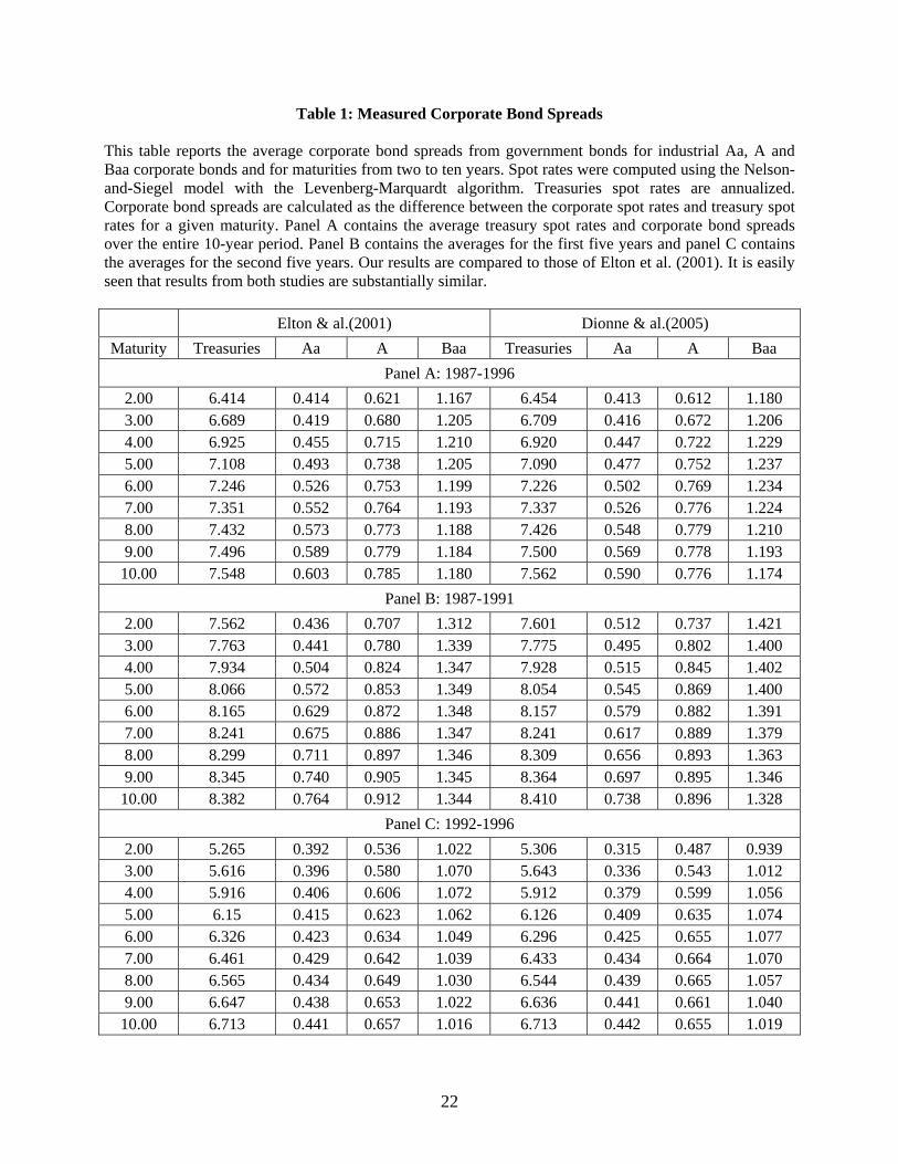
Table 1: Measured Corporate Bond Spreads This table reports the average corporate bond spreads from government bonds for industrial Aa, A and Baa corporate bonds and for maturities from two to ten years. Spot rates were computed using the Nelson-and-Siegel model with the Levenberg-Marquardt algorithm. Treasuries spot rates are annualized. Corporate bond spreads are calculated as the difference between the corporate spot rates and treasury spot rates for a given maturity. Panel A contains the average treasury spot rates and corporate bond spreads over the entire 10-year period. Panel B contains the averages for the first five years and panel C contains the averages for the second five years. Our results are compared to those of Elton et al. (2001). It is easily seen that results from both studies are substantially similar.

Elton & al.(2001) Dionne & al.(2005) Maturity Treasuries Aa A Baa Treasuries Aa A Baa

Panel A: 1987-1996 2.00 6.414 0.414 0.621 1.167 6.454 0.413 0.612 1.180 3.00 6.689 0.419 0.680 1.205 6.709 0.416 0.672 1.206 4.00 6.925 0.455 0.715 1.210 6.920 0.447 0.722 1.229 5.00 7.108 0.493 0.738 1.205 7.090 0.477 0.752 1.237 6.00 7.246 0.526 0.753 1.199 7.226 0.502 0.769 1.234 7.00 7.351 0.552 0.764 1.193 7.337 0.526 0.776 1.224 8.00 7.432 0.573 0.773 1.188 7.426 0.548 0.779 1.210 9.00 7.496 0.589 0.779 1.184 7.500 0.569 0.778 1.193

10.00 7.548 0.603 0.785 1.180 7.562 0.590 0.776 1.174 Panel B: 1987-1991

2.00 7.562 0.436 0.707 1.312 7.601 0.512 0.737 1.421 3.00 7.763 0.441 0.780 1.339 7.775 0.495 0.802 1.400 4.00 7.934 0.504 0.824 1.347 7.928 0.515 0.845 1.402 5.00 8.066 0.572 0.853 1.349 8.054 0.545 0.869 1.400 6.00 8.165 0.629 0.872 1.348 8.157 0.579 0.882 1.391 7.00 8.241 0.675 0.886 1.347 8.241 0.617 0.889 1.379 8.00 8.299 0.711 0.897 1.346 8.309 0.656 0.893 1.363 9.00 8.345 0.740 0.905 1.345 8.364 0.697 0.895 1.346

10.00 8.382 0.764 0.912 1.344 8.410 0.738 0.896 1.328 Panel C: 1992-1996

2.00 5.265 0.392 0.536 1.022 5.306 0.315 0.487 0.939 3.00 5.616 0.396 0.580 1.070 5.643 0.336 0.543 1.012 4.00 5.916 0.406 0.606 1.072 5.912 0.379 0.599 1.056 5.00 6.15 0.415 0.623 1.062 6.126 0.409 0.635 1.074 6.00 6.326 0.423 0.634 1.049 6.296 0.425 0.655 1.077 7.00 6.461 0.429 0.642 1.039 6.433 0.434 0.664 1.070 8.00 6.565 0.434 0.649 1.030 6.544 0.439 0.665 1.057 9.00 6.647 0.438 0.653 1.022 6.636 0.441 0.661 1.040

10.00 6.713 0.441 0.657 1.016 6.713 0.442 0.655 1.019

22

Table 2: Comparison of Average Root Mean Squared Errors

This table presents the average root mean squared error (ARMSE) of the difference between theoretical

bond prices computed using the Nelson-and-Siegel model and the actual bond prices for treasuries and

industrial Aa, A and Baa corporate bonds. The estimation procedure is described in Section 2. Root mean

squared error is measured in cents per dollar. For a given class of bonds, the root mean squared error is

calculated once per period (month). The number reported is the average of all root mean squared errors

within a given class over the months of the corresponding period. Our results are compared to those of

Elton et al. (2001). Again, the results are similar. The ARMSE formula is given below:

2

1

1

( ˆ )jn

i imi

j jA R M S E

P P

nm

=

==

−∑∑

where:

m: Number of months in the period.

nj: Number of bonds in month j.

iP : The theoretical price of bond i.

iP : The actual price of bond i.

Elton & al.(2001) Dionne & al.(2005)

Period Treasuries Aa A Baa Treasuries Aa A Baa 1987-1996 0.210 0.728 0.874 1.512 0.220 0.525 0.812 1.458 1987-1991 0.185 0.728 0.948 1.480 0.304 0.555 0.876 1.387 1992-1996 0.234 0.727 0.800 1.552 0.136 0.496 0.748 1.529

23

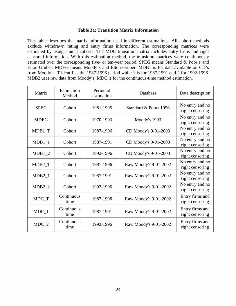
Table 3a: Transition Matrix Information This table describes the matrix information used in different estimations. All cohort methods exclude withdrawn rating and entry firms information. The corresponding matrices were estimated by using annual cohorts. The MDC transition matrix includes entry firms and right censored information. With this estimation method, the transition matrices were continuously estimated over the corresponding five- or ten-year period. SPEG means Standard & Poor’s and Elton-Gruber. MDEG means Moody’s and Elton-Gruber. MDB1 is for data available on CD’s from Moody’s. T identifies the 1987-1996 period while 1 is for 1987-1991 and 2 for 1992-1996. MDB2 uses raw data from Moody’s. MDC is for the continuous-time method estimation.

Matrix Estimation Method

Period of estimation Database Data description

SPEG Cohort 1981-1995 Standard & Poors 1996 No entry and no right censoring

MDEG Cohort 1970-1993 Moody's 1993 No entry and no right censoring

MDB1_T Cohort 1987-1996 CD Moody's 9-01-2003 No entry and no right censoring

MDB1_1 Cohort 1987-1991 CD Moody's 9-01-2003 No entry and no right censoring

MDB1_2 Cohort 1992-1996 CD Moody's 9-01-2003 No entry and no right censoring

MDB2_T Cohort 1987-1996 Raw Moody's 9-01-2002 No entry and no right censoring

MDB2_1 Cohort 1987-1991 Raw Moody's 9-01-2002 No entry and no right censoring

MDB2_2 Cohort 1992-1996 Raw Moody's 9-01-2002 No entry and no right censoring

MDC_T Continuous time 1987-1996 Raw Moody's 9-01-2002 Entry firms and

right censoring

MDC_1 Continuous time 1987-1991 Raw Moody's 9-01-2002 Entry firms and

right censoring

MDC_2 Continuous time 1992-1996 Raw Moody's 9-01-2002 Entry firms and

right censoring

24

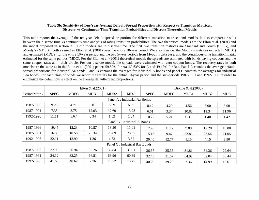
Table 3b: Sensitivity of Ten-Year Average Default-Spread Proportion with Respect to Transition Matrices, Discrete- vs Continuous-Time Transition Probabilities and Discrete Theoretical Models

This table reports the average of the ten-year default-spread proportion for different transition matrices and models. It also compares results between the discrete-time vs continuous-time analysis of rating transition probabilities. The two theoretical models are the Elton et al. (2001) and the model proposed in section 3.1. Both models are in discrete time. The first two transition matrices are Standard and Poor’s (SPEG), and Moody’s (MDEG), both as used in Elton et al. (2001) over the entire 10-year period. We also consider the Moody’s matrices extracted (MDB1) and estimated (MDB2) for the entire 10-year period and the two 5-year periods from Moody’s data base, and the continuous-time transition matrix estimated for the same periods (MDC). For the Elton et al. (2001) theoretical model, the spreads are estimated with bonds paying coupons and the same coupon rates as in their article. For our discrete model, the spreads were estimated with zero-coupon bonds. The recovery rates in both models are the same as in the Elton et al. (2001) paper: 59.59% for Aa, 60.63% for A and 49.42% for Baa. Panel A contains the average default-spread proportions for industrial Aa bonds. Panel B contains the averages for industrial A bonds and panel C contains the averages for industrial Baa bonds. For each class of bonds we report the results for the entire 10-year period and the sub-periods 1987-1991 and 1992-1996 in order to emphasize the default cycle effect on the average default-spread proportions.

Elton & al.(2001) Dionne & al.(2005)

Period/Matrix SPEG MDEG MDB1 MDB2 MDC SPEG MDEG MDB1 MDB2 MDCPanel A : Industrial Aa Bonds

1987-1996 9.23 4.71 5.01 6.59 6.59 8.42 4.29 4.56 6.00 6.001987-1991 7.35 3.75 12.03 12.60 13.28 6.61 3.37 10.82 11.34 11.961992-1996 11.11 5.67 0.34 1.52 1.54 10.22 5.21 0.31 1.40 1.42

Panel B : Industrial A Bonds 1987-1996 19.45 12.23 10.87 13.50 11.01 17.76 11.12 9.88 12.28 10.001987-1991 16.80 10.56 25.34 26.09 23.35 15.13 9.47 22.85 23.54 21.051992-1996 22.11 13.90 1.26 4.53 3.82 20.40 12.77 1.15 4.15 3.50

Panel C : Industrial Baa Bonds 1987-1996 37.90 36.94 33.26 35.84 31.01 36.37 35.38 31.81 34.36 29.641987-1991 34.12 33.25 66.81 63.96 60.39 32.45 31.57 64.92 62.04 58.441992-1996 41.68 40.62 7.76 15.72 13.25 40.29 39.20 7.36 14.99 12.61

25

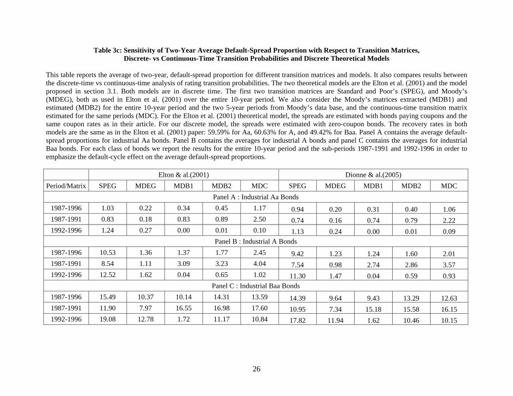
Table 3c: Sensitivity of Two-Year Average Default-Spread Proportion with Respect to Transition Matrices, Discrete- vs Continuous-Time Transition Probabilities and Discrete Theoretical Models

This table reports the average of two-year, default-spread proportion for different transition matrices and models. It also compares results between the discrete-time vs continuous-time analysis of rating transition probabilities. The two theoretical models are the Elton et al. (2001) and the model proposed in section 3.1. Both models are in discrete time. The first two transition matrices are Standard and Poor’s (SPEG), and Moody’s (MDEG), both as used in Elton et al. (2001) over the entire 10-year period. We also consider the Moody’s matrices extracted (MDB1) and estimated (MDB2) for the entire 10-year period and the two 5-year periods from Moody’s data base, and the continuous-time transition matrix estimated for the same periods (MDC). For the Elton et al. (2001) theoretical model, the spreads are estimated with bonds paying coupons and the same coupon rates as in their article. For our discrete model, the spreads were estimated with zero-coupon bonds. The recovery rates in both models are the same as in the Elton et al. (2001) paper: 59.59% for Aa, 60.63% for A, and 49.42% for Baa. Panel A contains the average default-spread proportions for industrial Aa bonds. Panel B contains the averages for industrial A bonds and panel C contains the averages for industrial Baa bonds. For each class of bonds we report the results for the entire 10-year period and the sub-periods 1987-1991 and 1992-1996 in order to emphasize the default-cycle effect on the average default-spread proportions.

Elton & al.(2001) Dionne & al.(2005) Period/Matrix SPEG MDEG MDB1 MDB2 MDC SPEG MDEG MDB1 MDB2 MDC

Panel A : Industrial Aa Bonds 1987-1996 1.03 0.22 0.34 0.45 1.17 0.94 0.20 0.31 0.40 1.061987-1991 0.83 0.18 0.83 0.89 2.50 0.74 0.16 0.74 0.79 2.221992-1996 1.24 0.27 0.00 0.01 0.10 1.13 0.24 0.00 0.01 0.09

Panel B : Industrial A Bonds 1987-1996 10.53 1.36 1.37 1.77 2.45 9.42 1.23 1.24 1.60 2.011987-1991 8.54 1.11 3.09 3.23 4.04 7.54 0.98 2.74 2.86 3.571992-1996 12.52 1.62 0.04 0.65 1.02 11.30 1.47 0.04 0.59 0.93

Panel C : Industrial Baa Bonds 1987-1996 15.49 10.37 10.14 14.31 13.59 14.39 9.64 9.43 13.29 12.631987-1991 11.90 7.97 16.55 16.98 17.60 10.95 7.34 15.18 15.58 16.151992-1996 19.08 12.78 1.72 11.17 10.84 17.82 11.94 1.62 10.46 10.15

26

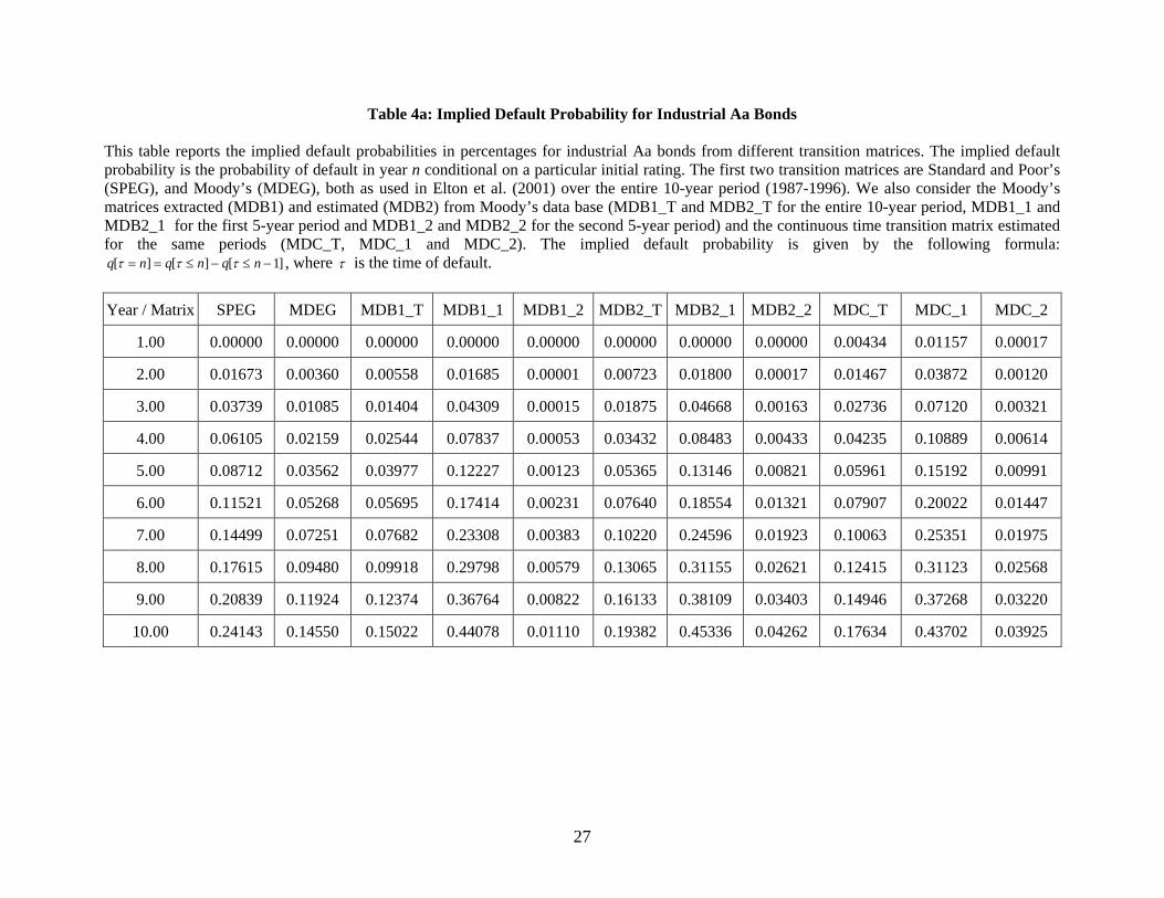
Table 4a: Implied Default Probability for Industrial Aa Bonds This table reports the implied default probabilities in percentages for industrial Aa bonds from different transition matrices. The implied default probability is the probability of default in year n conditional on a particular initial rating. The first two transition matrices are Standard and Poor’s (SPEG), and Moody’s (MDEG), both as used in Elton et al. (2001) over the entire 10-year period (1987-1996). We also consider the Moody’s matrices extracted (MDB1) and estimated (MDB2) from Moody’s data base (MDB1_T and MDB2_T for the entire 10-year period, MDB1_1 and MDB2_1 for the first 5-year period and MDB1_2 and MDB2_2 for the second 5-year period) and the continuous time transition matrix estimated for the same periods (MDC_T, MDC_1 and MDC_2). The implied default probability is given by the following formula:

[ ] [ ] [ 1]q n q n q nτ τ τ= = ≤ − ≤ − , where τ is the time of default. Year / Matrix SPEG MDEG MDB1_T MDB1_1 MDB1_2 MDB2_T MDB2_1 MDB2_2 MDC_T MDC_1 MDC_2

1.00 0.00000 0.00000 0.00000 0.00000 0.00000 0.00000 0.00000 0.00000 0.00434 0.01157 0.00017

2.00 0.01673 0.00360 0.00558 0.01685 0.00001 0.00723 0.01800 0.00017 0.01467 0.03872 0.00120

3.00 0.03739 0.01085 0.01404 0.04309 0.00015 0.01875 0.04668 0.00163 0.02736 0.07120 0.00321

4.00 0.06105 0.02159 0.02544 0.07837 0.00053 0.03432 0.08483 0.00433 0.04235 0.10889 0.00614

5.00 0.08712 0.03562 0.03977 0.12227 0.00123 0.05365 0.13146 0.00821 0.05961 0.15192 0.00991

6.00 0.11521 0.05268 0.05695 0.17414 0.00231 0.07640 0.18554 0.01321 0.07907 0.20022 0.01447

7.00 0.14499 0.07251 0.07682 0.23308 0.00383 0.10220 0.24596 0.01923 0.10063 0.25351 0.01975

8.00 0.17615 0.09480 0.09918 0.29798 0.00579 0.13065 0.31155 0.02621 0.12415 0.31123 0.02568

9.00 0.20839 0.11924 0.12374 0.36764 0.00822 0.16133 0.38109 0.03403 0.14946 0.37268 0.03220

10.00 0.24143 0.14550 0.15022 0.44078 0.01110 0.19382 0.45336 0.04262 0.17634 0.43702 0.03925

27

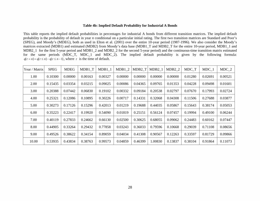
Table 4b: Implied Default Probability for Industrial A Bonds This table reports the implied default probabilities in percentages for industrial A bonds from different transition matrices. The implied default probability is the probability of default in year n conditional on a particular initial rating. The first two transition matrices are Standard and Poor’s (SPEG), and Moody’s (MDEG), both as used in Elton et al. (2001) over the entire 10-year period (1987-1996). We also consider the Moody’s matrices extracted (MDB1) and estimated (MDB2) from Moody’s data base (MDB1_T and MDB2_T for the entire 10-year period, MDB1_1 and MDB2_1 for the first 5-year period and MDB1_2 and MDB2_2 for the second 5-year period) and the continuous-time transition matrix estimated for the same periods (MDC_T, MDC_1 and MDC_2). The implied default probability is given by the following formula:

[ ] [ ] [ 1]q n q n q nτ τ τ= = ≤ − ≤ − , where τ is the time of default. Year / Matrix SPEG MDEG MDB1_T MDB1_1 MDB1_2 MDB2_T MDB2_1 MDB2_2 MDC_T MDC_1 MDC_2

1.00 0.10300 0.00000 0.00163 0.00327 0.00000 0.00000 0.00000 0.00000 0.01280 0.02691 0.00521

2.00 0.15435 0.03354 0.03215 0.09025 0.00086 0.04365 0.09765 0.01353 0.04228 0.09498 0.01601

3.00 0.20388 0.07442 0.06830 0.19102 0.00332 0.09184 0.20538 0.02797 0.07670 0.17993 0.02724

4.00 0.25321 0.12086 0.10895 0.30226 0.00717 0.14331 0.32068 0.04308 0.11506 0.27688 0.03877

5.00 0.30273 0.17126 0.15296 0.42013 0.01219 0.19688 0.44035 0.05867 0.15643 0.38174 0.05053

6.00 0.35223 0.22417 0.19920 0.54090 0.01819 0.25151 0.56124 0.07457 0.19994 0.49100 0.06244

7.00 0.40119 0.27833 0.24662 0.66130 0.02500 0.30625 0.68055 0.09062 0.24483 0.60162 0.07447

8.00 0.44905 0.33264 0.29432 0.77858 0.03243 0.36033 0.79596 0.10668 0.29039 0.71108 0.08656

9.00 0.49526 0.38622 0.34154 0.89059 0.04034 0.41308 0.90567 0.12263 0.33597 0.81729 0.09866

10.00 0.53935 0.43834 0.38763 0.99573 0.04859 0.46399 1.00830 0.13837 0.38104 0.91864 0.11073

28

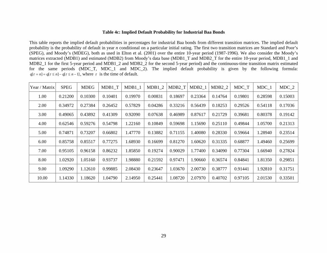
Table 4c: Implied Default Probability for Industrial Baa Bonds This table reports the implied default probabilities in percentages for industrial Baa bonds from different transition matrices. The implied default probability is the probability of default in year n conditional on a particular initial rating. The first two transition matrices are Standard and Poor’s (SPEG), and Moody’s (MDEG), both as used in Elton et al. (2001) over the entire 10-year period (1987-1996). We also consider the Moody’s matrices extracted (MDB1) and estimated (MDB2) from Moody’s data base (MDB1_T and MDB2_T for the entire 10-year period, MDB1_1 and MDB2_1 for the first 5-year period and MDB1_2 and MDB2_2 for the second 5-year period) and the continuous-time transition matrix estimated for the same periods (MDC_T, MDC_1 and MDC_2). The implied default probability is given by the following formula:

[ ] [ ] [ 1]q n q n q nτ τ τ= = ≤ − ≤ − , where τ is the time of default. Year / Matrix SPEG MDEG MDB1_T MDB1_1 MDB1_2 MDB2_T MDB2_1 MDB2_2 MDC_T MDC_1 MDC_2

1.00 0.21200 0.10300 0.10401 0.19970 0.00831 0.18697 0.23364 0.14764 0.19801 0.28598 0.15003

2.00 0.34972 0.27384 0.26452 0.57829 0.04286 0.33216 0.56439 0.18253 0.29526 0.54118 0.17036

3.00 0.49065 0.43892 0.41309 0.92090 0.07638 0.46989 0.87617 0.21729 0.39681 0.80378 0.19142

4.00 0.62546 0.59276 0.54798 1.22160 0.10849 0.59698 1.15690 0.25110 0.49844 1.05700 0.21313

5.00 0.74871 0.73207 0.66802 1.47770 0.13882 0.71155 1.40080 0.28330 0.59664 1.28940 0.23514

6.00 0.85758 0.85517 0.77275 1.68930 0.16699 0.81270 1.60620 0.31335 0.68877 1.49460 0.25699

7.00 0.95105 0.96158 0.86232 1.85850 0.19274 0.90029 1.77400 0.34090 0.77304 1.66940 0.27824

8.00 1.02920 1.05160 0.93737 1.98880 0.21592 0.97471 1.90660 0.36574 0.84841 1.81350 0.29851

9.00 1.09290 1.12610 0.99885 2.08430 0.23647 1.03670 2.00730 0.38777 0.91441 1.92810 0.31751

10.00 1.14330 1.18620 1.04790 2.14950 0.25441 1.08720 2.07970 0.40702 0.97105 2.01530 0.33501

29

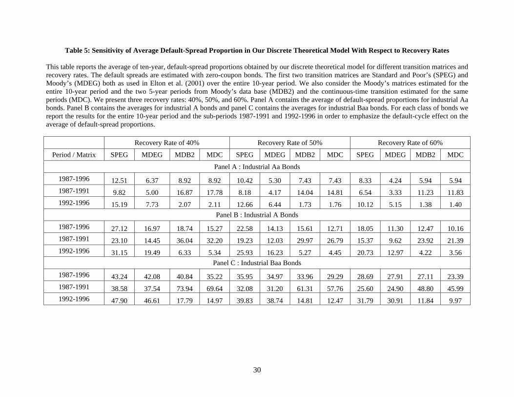
Table 5: Sensitivity of Average Default-Spread Proportion in Our Discrete Theoretical Model With Respect to Recovery Rates This table reports the average of ten-year, default-spread proportions obtained by our discrete theoretical model for different transition matrices and recovery rates. The default spreads are estimated with zero-coupon bonds. The first two transition matrices are Standard and Poor’s (SPEG) and Moody’s (MDEG) both as used in Elton et al. (2001) over the entire 10-year period. We also consider the Moody’s matrices estimated for the entire 10-year period and the two 5-year periods from Moody’s data base (MDB2) and the continuous-time transition estimated for the same periods (MDC). We present three recovery rates: 40%, 50%, and 60%. Panel A contains the average of default-spread proportions for industrial Aa bonds. Panel B contains the averages for industrial A bonds and panel C contains the averages for industrial Baa bonds. For each class of bonds we report the results for the entire 10-year period and the sub-periods 1987-1991 and 1992-1996 in order to emphasize the default-cycle effect on the average of default-spread proportions.

Recovery Rate of 40% Recovery Rate of 50% Recovery Rate of 60%

Period / Matrix SPEG MDEG MDB2 MDC SPEG MDEG MDB2 MDC SPEG MDEG MDB2 MDC

Panel A : Industrial Aa Bonds

1987-1996 12.51 6.37 8.92 8.92 10.42 5.30 7.43 7.43 8.33 4.24 5.94 5.941987-1991 9.82 5.00 16.87 17.78 8.18 4.17 14.04 14.81 6.54 3.33 11.23 11.831992-1996 15.19 7.73 2.07 2.11 12.66 6.44 1.73 1.76 10.12 5.15 1.38 1.40

Panel B : Industrial A Bonds

1987-1996 27.12 16.97 18.74 15.27 22.58 14.13 15.61 12.71 18.05 11.30 12.47 10.161987-1991 23.10 14.45 36.04 32.20 19.23 12.03 29.97 26.79 15.37 9.62 23.92 21.391992-1996 31.15 19.49 6.33 5.34 25.93 16.23 5.27 4.45 20.73 12.97 4.22 3.56

Panel C : Industrial Baa Bonds

1987-1996 43.24 42.08 40.84 35.22 35.95 34.97 33.96 29.29 28.69 27.91 27.11 23.391987-1991 38.58 37.54 73.94 69.64 32.08 31.20 61.31 57.76 25.60 24.90 48.80 45.991992-1996 47.90 46.61 17.79 14.97 39.83 38.74 14.81 12.47 31.79 30.91 11.84 9.97

30

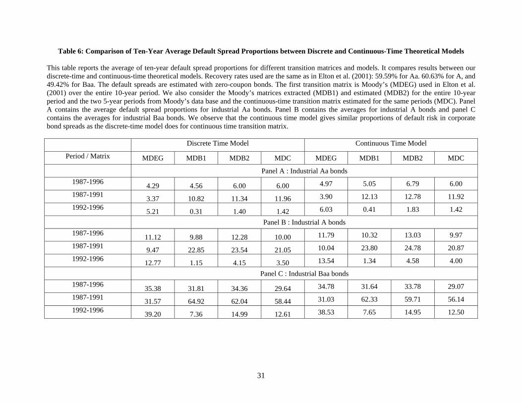
Table 6: Comparison of Ten-Year Average Default Spread Proportions between Discrete and Continuous-Time Theoretical Models This table reports the average of ten-year default spread proportions for different transition matrices and models. It compares results between our discrete-time and continuous-time theoretical models. Recovery rates used are the same as in Elton et al. (2001): 59.59% for Aa. 60.63% for A, and 49.42% for Baa. The default spreads are estimated with zero-coupon bonds. The first transition matrix is Moody’s (MDEG) used in Elton et al. (2001) over the entire 10-year period. We also consider the Moody’s matrices extracted (MDB1) and estimated (MDB2) for the entire 10-year period and the two 5-year periods from Moody’s data base and the continuous-time transition matrix estimated for the same periods (MDC). Panel A contains the average default spread proportions for industrial Aa bonds. Panel B contains the averages for industrial A bonds and panel C contains the averages for industrial Baa bonds. We observe that the continuous time model gives similar proportions of default risk in corporate bond spreads as the discrete-time model does for continuous time transition matrix.

Discrete Time Model Continuous Time Model

Period / Matrix MDEG MDB1 MDB2 MDC MDEG MDB1 MDB2 MDC Panel A : Industrial Aa bonds

1987-1996 4.29 4.56 6.00 6.00 4.97 5.05 6.79 6.001987-1991 3.37 10.82 11.34 11.96 3.90 12.13 12.78 11.921992-1996 5.21 0.31 1.40 1.42 6.03 0.41 1.83 1.42

Panel B : Industrial A bonds 1987-1996 11.12 9.88 12.28 10.00 11.79 10.32 13.03 9.971987-1991 9.47 22.85 23.54 21.05 10.04 23.80 24.78 20.871992-1996 12.77 1.15 4.15 3.50 13.54 1.34 4.58 4.00

Panel C : Industrial Baa bonds 1987-1996 35.38 31.81 34.36 29.64 34.78 31.64 33.78 29.071987-1991 31.57 64.92 62.04 58.44 31.03 62.33 59.71 56.141992-1996 39.20 7.36 14.99 12.61 38.53 7.65 14.95 12.50

31

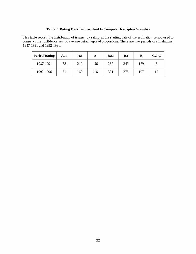
Table 7: Rating Distributions Used to Compute Descriptive Statistics

This table reports the distribution of issuers, by rating, at the starting date of the estimation period used to construct the confidence sets of average default-spread proportions. There are two periods of simulations: 1987-1991 and 1992-1996.

Period/Rating Aaa Aa A Baa Ba B CC-C

1987-1991 58 210 456 287 343 179 6

1992-1996 51 160 416 321 275 197 12

32

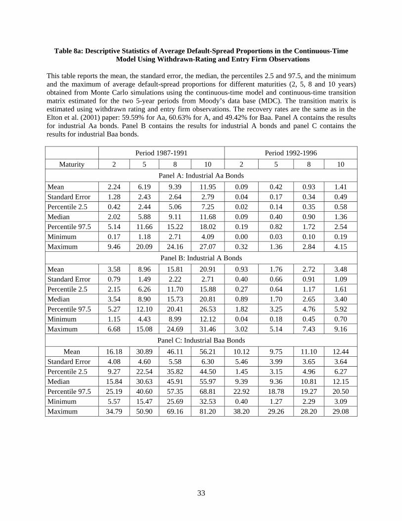
Table 8a: Descriptive Statistics of Average Default-Spread Proportions in the Continuous-Time Model Using Withdrawn-Rating and Entry Firm Observations

This table reports the mean, the standard error, the median, the percentiles 2.5 and 97.5, and the minimum and the maximum of average default-spread proportions for different maturities (2, 5, 8 and 10 years) obtained from Monte Carlo simulations using the continuous-time model and continuous-time transition matrix estimated for the two 5-year periods from Moody’s data base (MDC). The transition matrix is estimated using withdrawn rating and entry firm observations. The recovery rates are the same as in the Elton et al. (2001) paper: 59.59% for Aa, 60.63% for A, and 49.42% for Baa. Panel A contains the results for industrial Aa bonds. Panel B contains the results for industrial A bonds and panel C contains the results for industrial Baa bonds.

Period 1987-1991 Period 1992-1996 Maturity 2 5 8 10 2 5 8 10

Panel A: Industrial Aa Bonds Mean 2.24 6.19 9.39 11.95 0.09 0.42 0.93 1.41 Standard Error 1.28 2.43 2.64 2.79 0.04 0.17 0.34 0.49 Percentile 2.5 0.42 2.44 5.06 7.25 0.02 0.14 0.35 0.58 Median 2.02 5.88 9.11 11.68 0.09 0.40 0.90 1.36 Percentile 97.5 5.14 11.66 15.22 18.02 0.19 0.82 1.72 2.54 Minimum 0.17 1.18 2.71 4.09 0.00 0.03 0.10 0.19 Maximum 9.46 20.09 24.16 27.07 0.32 1.36 2.84 4.15

Panel B: Industrial A Bonds Mean 3.58 8.96 15.81 20.91 0.93 1.76 2.72 3.48 Standard Error 0.79 1.49 2.22 2.71 0.40 0.66 0.91 1.09 Percentile 2.5 2.15 6.26 11.70 15.88 0.27 0.64 1.17 1.61 Median 3.54 8.90 15.73 20.81 0.89 1.70 2.65 3.40 Percentile 97.5 5.27 12.10 20.41 26.53 1.82 3.25 4.76 5.92 Minimum 1.15 4.43 8.99 12.12 0.04 0.18 0.45 0.70 Maximum 6.68 15.08 24.69 31.46 3.02 5.14 7.43 9.16

Panel C: Industrial Baa Bonds Mean 16.18 30.89 46.11 56.21 10.12 9.75 11.10 12.44

Standard Error 4.08 4.60 5.58 6.30 5.46 3.99 3.65 3.64 Percentile 2.5 9.27 22.54 35.82 44.50 1.45 3.15 4.96 6.27 Median 15.84 30.63 45.91 55.97 9.39 9.36 10.81 12.15 Percentile 97.5 25.19 40.60 57.35 68.81 22.92 18.78 19.27 20.50 Minimum 5.57 15.47 25.69 32.53 0.40 1.27 2.29 3.09 Maximum 34.79 50.90 69.16 81.20 38.20 29.26 28.20 29.08

33

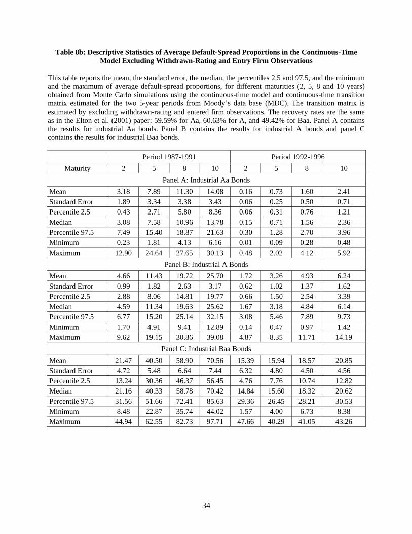
Table 8b: Descriptive Statistics of Average Default-Spread Proportions in the Continuous-Time Model Excluding Withdrawn-Rating and Entry Firm Observations

This table reports the mean, the standard error, the median, the percentiles 2.5 and 97.5, and the minimum and the maximum of average default-spread proportions, for different maturities (2, 5, 8 and 10 years) obtained from Monte Carlo simulations using the continuous-time model and continuous-time transition matrix estimated for the two 5-year periods from Moody’s data base (MDC). The transition matrix is estimated by excluding withdrawn-rating and entered firm observations. The recovery rates are the same as in the Elton et al. (2001) paper: 59.59% for Aa, 60.63% for A, and 49.42% for Baa. Panel A contains the results for industrial Aa bonds. Panel B contains the results for industrial A bonds and panel C contains the results for industrial Baa bonds.

Period 1987-1991 Period 1992-1996 Maturity 2 5 8 10 2 5 8 10

Panel A: Industrial Aa Bonds Mean 3.18 7.89 11.30 14.08 0.16 0.73 1.60 2.41 Standard Error 1.89 3.34 3.38 3.43 0.06 0.25 0.50 0.71 Percentile 2.5 0.43 2.71 5.80 8.36 0.06 0.31 0.76 1.21 Median 3.08 7.58 10.96 13.78 0.15 0.71 1.56 2.36 Percentile 97.5 7.49 15.40 18.87 21.63 0.30 1.28 2.70 3.96 Minimum 0.23 1.81 4.13 6.16 0.01 0.09 0.28 0.48 Maximum 12.90 24.64 27.65 30.13 0.48 2.02 4.12 5.92

Panel B: Industrial A Bonds Mean 4.66 11.43 19.72 25.70 1.72 3.26 4.93 6.24 Standard Error 0.99 1.82 2.63 3.17 0.62 1.02 1.37 1.62 Percentile 2.5 2.88 8.06 14.81 19.77 0.66 1.50 2.54 3.39 Median 4.59 11.34 19.63 25.62 1.67 3.18 4.84 6.14 Percentile 97.5 6.77 15.20 25.14 32.15 3.08 5.46 7.89 9.73 Minimum 1.70 4.91 9.41 12.89 0.14 0.47 0.97 1.42 Maximum 9.62 19.15 30.86 39.08 4.87 8.35 11.71 14.19

Panel C: Industrial Baa Bonds Mean 21.47 40.50 58.90 70.56 15.39 15.94 18.57 20.85 Standard Error 4.72 5.48 6.64 7.44 6.32 4.80 4.50 4.56 Percentile 2.5 13.24 30.36 46.37 56.45 4.76 7.76 10.74 12.82 Median 21.16 40.33 58.78 70.42 14.84 15.60 18.32 20.62 Percentile 97.5 31.56 51.66 72.41 85.63 29.36 26.45 28.21 30.53 Minimum 8.48 22.87 35.74 44.02 1.57 4.00 6.73 8.38 Maximum 44.94 62.55 82.73 97.71 47.66 40.29 41.05 43.26

34

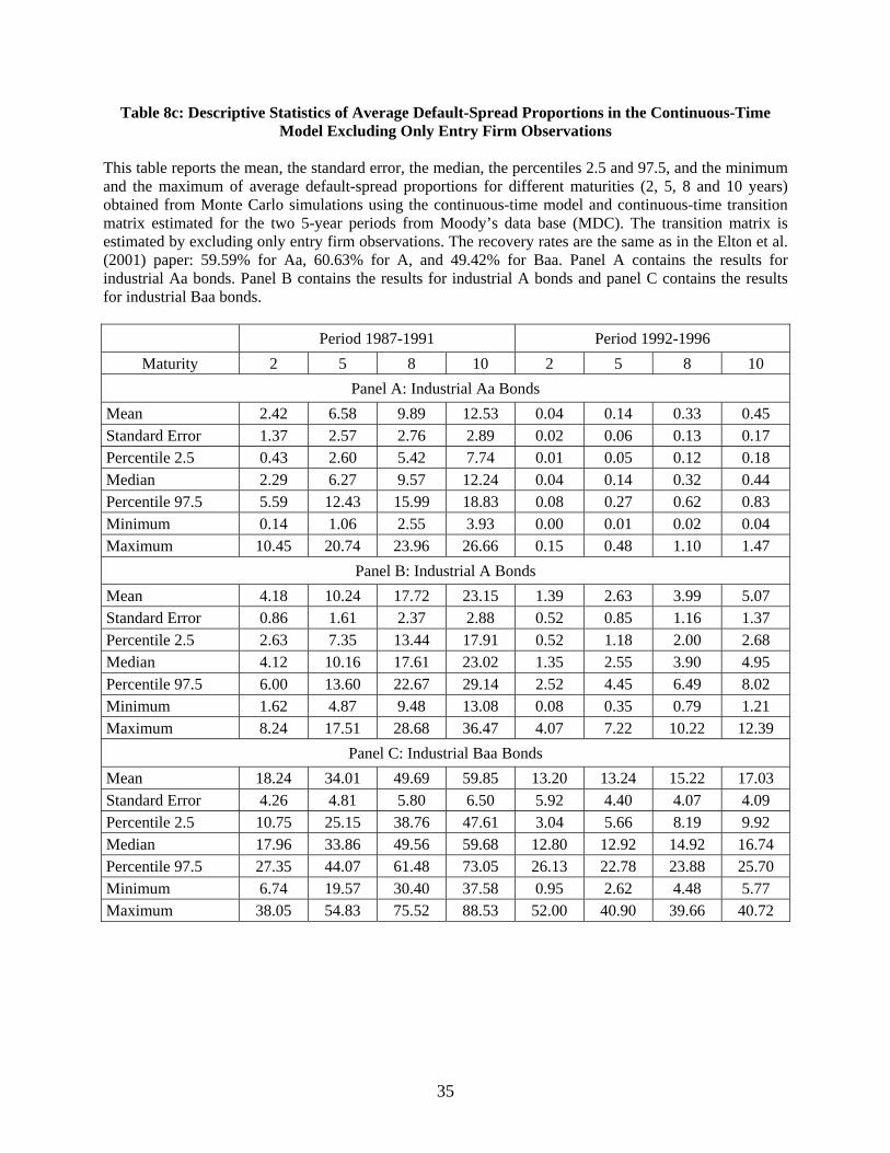
Table 8c: Descriptive Statistics of Average Default-Spread Proportions in the Continuous-Time Model Excluding Only Entry Firm Observations

This table reports the mean, the standard error, the median, the percentiles 2.5 and 97.5, and the minimum and the maximum of average default-spread proportions for different maturities (2, 5, 8 and 10 years) obtained from Monte Carlo simulations using the continuous-time model and continuous-time transition matrix estimated for the two 5-year periods from Moody’s data base (MDC). The transition matrix is estimated by excluding only entry firm observations. The recovery rates are the same as in the Elton et al. (2001) paper: 59.59% for Aa, 60.63% for A, and 49.42% for Baa. Panel A contains the results for industrial Aa bonds. Panel B contains the results for industrial A bonds and panel C contains the results for industrial Baa bonds.

Period 1987-1991 Period 1992-1996 Maturity 2 5 8 10 2 5 8 10

Panel A: Industrial Aa Bonds Mean 2.42 6.58 9.89 12.53 0.04 0.14 0.33 0.45 Standard Error 1.37 2.57 2.76 2.89 0.02 0.06 0.13 0.17 Percentile 2.5 0.43 2.60 5.42 7.74 0.01 0.05 0.12 0.18 Median 2.29 6.27 9.57 12.24 0.04 0.14 0.32 0.44 Percentile 97.5 5.59 12.43 15.99 18.83 0.08 0.27 0.62 0.83 Minimum 0.14 1.06 2.55 3.93 0.00 0.01 0.02 0.04 Maximum 10.45 20.74 23.96 26.66 0.15 0.48 1.10 1.47

Panel B: Industrial A Bonds Mean 4.18 10.24 17.72 23.15 1.39 2.63 3.99 5.07 Standard Error 0.86 1.61 2.37 2.88 0.52 0.85 1.16 1.37 Percentile 2.5 2.63 7.35 13.44 17.91 0.52 1.18 2.00 2.68 Median 4.12 10.16 17.61 23.02 1.35 2.55 3.90 4.95 Percentile 97.5 6.00 13.60 22.67 29.14 2.52 4.45 6.49 8.02 Minimum 1.62 4.87 9.48 13.08 0.08 0.35 0.79 1.21 Maximum 8.24 17.51 28.68 36.47 4.07 7.22 10.22 12.39

Panel C: Industrial Baa Bonds Mean 18.24 34.01 49.69 59.85 13.20 13.24 15.22 17.03 Standard Error 4.26 4.81 5.80 6.50 5.92 4.40 4.07 4.09 Percentile 2.5 10.75 25.15 38.76 47.61 3.04 5.66 8.19 9.92 Median 17.96 33.86 49.56 59.68 12.80 12.92 14.92 16.74 Percentile 97.5 27.35 44.07 61.48 73.05 26.13 22.78 23.88 25.70 Minimum 6.74 19.57 30.40 37.58 0.95 2.62 4.48 5.77 Maximum 38.05 54.83 75.52 88.53 52.00 40.90 39.66 40.72

35

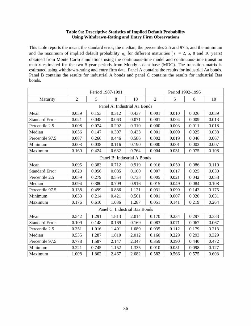
Table 9a: Descriptive Statistics of Implied Default Probability Using Withdrawn-Rating and Entry Firm Observations

This table reports the mean, the standard error, the median, the percentiles 2.5 and 97.5, and the minimum and the maximum of implied default probability sq for different maturities ( s = 2, 5, 8 and 10 years) obtained from Monte Carlo simulations using the continuous-time model and continuous-time transition matrix estimated for the two 5-year periods from Moody’s data base (MDC). The transition matrix is estimated using withdrawn-rating and entry firm data. Panel A contains the results for industrial Aa bonds. Panel B contains the results for industrial A bonds and panel C contains the results for industrial Baa bonds.

Period 1987-1991 Period 1992-1996 Maturity 2 5 8 10 2 5 8 10

Panel A: Industrial Aa Bonds Mean 0.039 0.153 0.312 0.437 0.001 0.010 0.026 0.039 Standard Error 0.021 0.048 0.063 0.071 0.001 0.004 0.009 0.013 Percentile 2.5 0.008 0.074 0.202 0.310 0.000 0.003 0.011 0.018 Median 0.036 0.147 0.307 0.433 0.001 0.009 0.025 0.038 Percentile 97.5 0.087 0.260 0.446 0.586 0.002 0.019 0.046 0.067 Minimum 0.003 0.038 0.116 0.190 0.000 0.001 0.003 0.007 Maximum 0.160 0.424 0.632 0.764 0.004 0.031 0.075 0.108

Panel B: Industrial A Bonds Mean 0.095 0.383 0.712 0.919 0.016 0.050 0.086 0.110 Standard Error 0.020 0.056 0.085 0.100 0.007 0.017 0.025 0.030 Percentile 2.5 0.059 0.279 0.554 0.733 0.005 0.021 0.042 0.058 Median 0.094 0.380 0.709 0.916 0.015 0.049 0.084 0.108 Percentile 97.5 0.138 0.499 0.886 1.121 0.031 0.090 0.143 0.175 Minimum 0.033 0.214 0.421 0.561 0.001 0.007 0.020 0.031 Maximum 0.176 0.610 1.036 1.287 0.051 0.141 0.219 0.264

Panel C: Industrial Baa Bonds Mean 0.542 1.291 1.813 2.014 0.170 0.234 0.297 0.333 Standard Error 0.109 0.148 0.169 0.169 0.083 0.071 0.067 0.067 Percentile 2.5 0.351 1.016 1.491 1.689 0.035 0.112 0.179 0.213 Median 0.535 1.287 1.810 2.012 0.160 0.229 0.293 0.329 Percentile 97.5 0.778 1.587 2.147 2.347 0.359 0.390 0.440 0.472 Minimum 0.221 0.745 1.152 1.335 0.010 0.051 0.098 0.127 Maximum 1.008 1.862 2.467 2.682 0.582 0.566 0.575 0.603

36

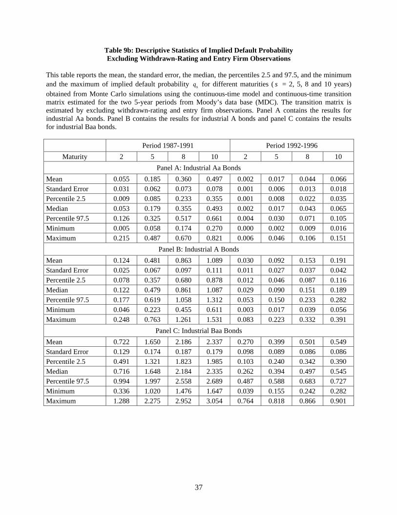
Table 9b: Descriptive Statistics of Implied Default Probability Excluding Withdrawn-Rating and Entry Firm Observations

This table reports the mean, the standard error, the median, the percentiles 2.5 and 97.5, and the minimum and the maximum of implied default probability sq for different maturities ( s = 2, 5, 8 and 10 years) obtained from Monte Carlo simulations using the continuous-time model and continuous-time transition matrix estimated for the two 5-year periods from Moody’s data base (MDC). The transition matrix is estimated by excluding withdrawn-rating and entry firm observations. Panel A contains the results for industrial Aa bonds. Panel B contains the results for industrial A bonds and panel C contains the results for industrial Baa bonds.

Period 1987-1991 Period 1992-1996 Maturity 2 5 8 10 2 5 8 10

Panel A: Industrial Aa Bonds Mean 0.055 0.185 0.360 0.497 0.002 0.017 0.044 0.066 Standard Error 0.031 0.062 0.073 0.078 0.001 0.006 0.013 0.018 Percentile 2.5 0.009 0.085 0.233 0.355 0.001 0.008 0.022 0.035 Median 0.053 0.179 0.355 0.493 0.002 0.017 0.043 0.065 Percentile 97.5 0.126 0.325 0.517 0.661 0.004 0.030 0.071 0.105 Minimum 0.005 0.058 0.174 0.270 0.000 0.002 0.009 0.016 Maximum 0.215 0.487 0.670 0.821 0.006 0.046 0.106 0.151

Panel B: Industrial A Bonds Mean 0.124 0.481 0.863 1.089 0.030 0.092 0.153 0.191 Standard Error 0.025 0.067 0.097 0.111 0.011 0.027 0.037 0.042 Percentile 2.5 0.078 0.357 0.680 0.878 0.012 0.046 0.087 0.116 Median 0.122 0.479 0.861 1.087 0.029 0.090 0.151 0.189 Percentile 97.5 0.177 0.619 1.058 1.312 0.053 0.150 0.233 0.282 Minimum 0.046 0.223 0.455 0.611 0.003 0.017 0.039 0.056 Maximum 0.248 0.763 1.261 1.531 0.083 0.223 0.332 0.391

Panel C: Industrial Baa Bonds Mean 0.722 1.650 2.186 2.337 0.270 0.399 0.501 0.549 Standard Error 0.129 0.174 0.187 0.179 0.098 0.089 0.086 0.086 Percentile 2.5 0.491 1.321 1.823 1.985 0.103 0.240 0.342 0.390 Median 0.716 1.648 2.184 2.335 0.262 0.394 0.497 0.545 Percentile 97.5 0.994 1.997 2.558 2.689 0.487 0.588 0.683 0.727 Minimum 0.336 1.020 1.476 1.647 0.039 0.155 0.242 0.282 Maximum 1.288 2.275 2.952 3.054 0.764 0.818 0.866 0.901

37

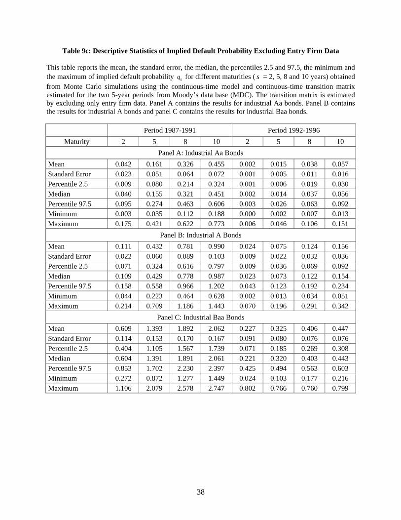
Table 9c: Descriptive Statistics of Implied Default Probability Excluding Entry Firm Data This table reports the mean, the standard error, the median, the percentiles 2.5 and 97.5, the minimum and the maximum of implied default probability sq for different maturities ( s = 2, 5, 8 and 10 years) obtained from Monte Carlo simulations using the continuous-time model and continuous-time transition matrix estimated for the two 5-year periods from Moody’s data base (MDC). The transition matrix is estimated by excluding only entry firm data. Panel A contains the results for industrial Aa bonds. Panel B contains the results for industrial A bonds and panel C contains the results for industrial Baa bonds.

Period 1987-1991 Period 1992-1996 Maturity 2 5 8 10 2 5 8 10

Panel A: Industrial Aa Bonds Mean 0.042 0.161 0.326 0.455 0.002 0.015 0.038 0.057 Standard Error 0.023 0.051 0.064 0.072 0.001 0.005 0.011 0.016 Percentile 2.5 0.009 0.080 0.214 0.324 0.001 0.006 0.019 0.030 Median 0.040 0.155 0.321 0.451 0.002 0.014 0.037 0.056 Percentile 97.5 0.095 0.274 0.463 0.606 0.003 0.026 0.063 0.092 Minimum 0.003 0.035 0.112 0.188 0.000 0.002 0.007 0.013 Maximum 0.175 0.421 0.622 0.773 0.006 0.046 0.106 0.151

Panel B: Industrial A Bonds Mean 0.111 0.432 0.781 0.990 0.024 0.075 0.124 0.156 Standard Error 0.022 0.060 0.089 0.103 0.009 0.022 0.032 0.036 Percentile 2.5 0.071 0.324 0.616 0.797 0.009 0.036 0.069 0.092 Median 0.109 0.429 0.778 0.987 0.023 0.073 0.122 0.154 Percentile 97.5 0.158 0.558 0.966 1.202 0.043 0.123 0.192 0.234 Minimum 0.044 0.223 0.464 0.628 0.002 0.013 0.034 0.051 Maximum 0.214 0.709 1.186 1.443 0.070 0.196 0.291 0.342

Panel C: Industrial Baa Bonds Mean 0.609 1.393 1.892 2.062 0.227 0.325 0.406 0.447 Standard Error 0.114 0.153 0.170 0.167 0.091 0.080 0.076 0.076 Percentile 2.5 0.404 1.105 1.567 1.739 0.071 0.185 0.269 0.308 Median 0.604 1.391 1.891 2.061 0.221 0.320 0.403 0.443 Percentile 97.5 0.853 1.702 2.230 2.397 0.425 0.494 0.563 0.603 Minimum 0.272 0.872 1.277 1.449 0.024 0.103 0.177 0.216 Maximum 1.106 2.079 2.578 2.747 0.802 0.766 0.760 0.799

38

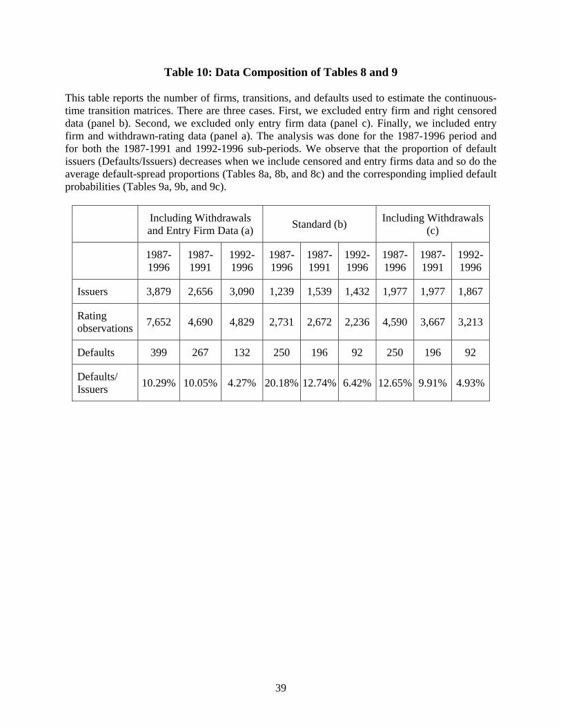
Table 10: Data Composition of Tables 8 and 9

This table reports the number of firms, transitions, and defaults used to estimate the continuous-time transition matrices. There are three cases. First, we excluded entry firm and right censored data (panel b). Second, we excluded only entry firm data (panel c). Finally, we included entry firm and withdrawn-rating data (panel a). The analysis was done for the 1987-1996 period and for both the 1987-1991 and 1992-1996 sub-periods. We observe that the proportion of default issuers (Defaults/Issuers) decreases when we include censored and entry firms data and so do the average default-spread proportions (Tables 8a, 8b, and 8c) and the corresponding implied default probabilities (Tables 9a, 9b, and 9c).

Including Withdrawals and Entry Firm Data (a) Standard (b) Including Withdrawals

(c)

1987-1996

1987-1991

1992-1996

1987-1996

1987-1991

1992-1996

1987-1996

1987-1991

1992-1996

Issuers 3,879 2,656 3,090 1,239 1,539 1,432 1,977 1,977 1,867

Rating observations 7,652 4,690 4,829 2,731 2,672 2,236 4,590 3,667 3,213

Defaults 399 267 132 250 196 92 250 196 92

Defaults/ Issuers 10.29% 10.05% 4.27% 20.18% 12.74% 6.42% 12.65% 9.91% 4.93%

39

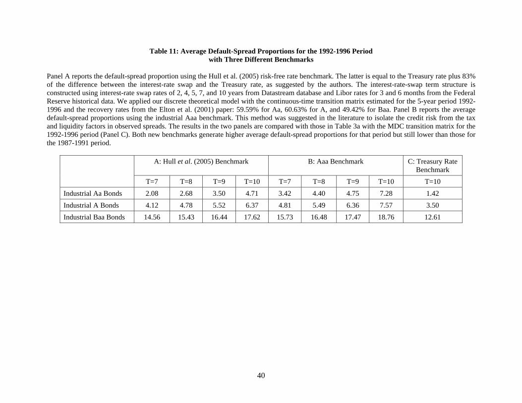
Table 11: Average Default-Spread Proportions for the 1992-1996 Period with Three Different Benchmarks

Panel A reports the default-spread proportion using the Hull et al. (2005) risk-free rate benchmark. The latter is equal to the Treasury rate plus 83% of the difference between the interest-rate swap and the Treasury rate, as suggested by the authors. The interest-rate-swap term structure is constructed using interest-rate swap rates of 2, 4, 5, 7, and 10 years from Datastream database and Libor rates for 3 and 6 months from the Federal Reserve historical data. We applied our discrete theoretical model with the continuous-time transition matrix estimated for the 5-year period 1992-1996 and the recovery rates from the Elton et al. (2001) paper: 59.59% for Aa, 60.63% for A, and 49.42% for Baa. Panel B reports the average default-spread proportions using the industrial Aaa benchmark. This method was suggested in the literature to isolate the credit risk from the tax and liquidity factors in observed spreads. The results in the two panels are compared with those in Table 3a with the MDC transition matrix for the 1992-1996 period (Panel C). Both new benchmarks generate higher average default-spread proportions for that period but still lower than those for the 1987-1991 period.

A: Hull et al. (2005) Benchmark B: Aaa Benchmark C: Treasury Rate Benchmark

T=7 T=8 T=9 T=10 T=7 T=8 T=9 T=10 T=10 Industrial Aa Bonds 2.08 2.68 3.50 4.71 3.42 4.40 4.75 7.28 1.42 Industrial A Bonds 4.12 4.78 5.52 6.37 4.81 5.49 6.36 7.57 3.50 Industrial Baa Bonds 14.56 15.43 16.44 17.62 15.73 16.48 17.47 18.76 12.61

40

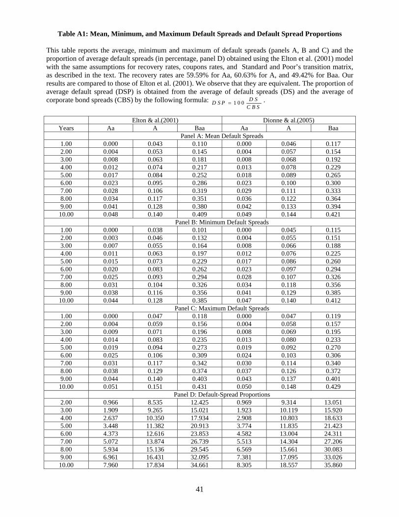
Table A1: Mean, Minimum, and Maximum Default Spreads and Default Spread Proportions This table reports the average, minimum and maximum of default spreads (panels A, B and C) and the proportion of average default spreads (in percentage, panel D) obtained using the Elton et al. (2001) model with the same assumptions for recovery rates, coupons rates, and Standard and Poor’s transition matrix, as described in the text. The recovery rates are 59.59% for Aa, 60.63% for A, and 49.42% for Baa. Our results are compared to those of Elton et al. (2001). We observe that they are equivalent. The proportion of average default spread (DSP) is obtained from the average of default spreads (DS) and the average of corporate bond spreads (CBS) by the following formula: 1 0 0 D SD S P

C B S= .

Elton & al.(2001) Dionne & al.(2005)

Years Aa A Baa Aa A Baa Panel A: Mean Default Spreads

1.00 0.000 0.043 0.110 0.000 0.046 0.117 2.00 0.004 0.053 0.145 0.004 0.057 0.154 3.00 0.008 0.063 0.181 0.008 0.068 0.192 4.00 0.012 0.074 0.217 0.013 0.078 0.229 5.00 0.017 0.084 0.252 0.018 0.089 0.265 6.00 0.023 0.095 0.286 0.023 0.100 0.300 7.00 0.028 0.106 0.319 0.029 0.111 0.333 8.00 0.034 0.117 0.351 0.036 0.122 0.364 9.00 0.041 0.128 0.380 0.042 0.133 0.394 10.00 0.048 0.140 0.409 0.049 0.144 0.421

Panel B: Minimum Default Spreads 1.00 0.000 0.038 0.101 0.000 0.045 0.115 2.00 0.003 0.046 0.132 0.004 0.055 0.151 3.00 0.007 0.055 0.164 0.008 0.066 0.188 4.00 0.011 0.063 0.197 0.012 0.076 0.225 5.00 0.015 0.073 0.229 0.017 0.086 0.260 6.00 0.020 0.083 0.262 0.023 0.097 0.294 7.00 0.025 0.093 0.294 0.028 0.107 0.326 8.00 0.031 0.104 0.326 0.034 0.118 0.356 9.00 0.038 0.116 0.356 0.041 0.129 0.385 10.00 0.044 0.128 0.385 0.047 0.140 0.412

Panel C: Maximum Default Spreads 1.00 0.000 0.047 0.118 0.000 0.047 0.119 2.00 0.004 0.059 0.156 0.004 0.058 0.157 3.00 0.009 0.071 0.196 0.008 0.069 0.195 4.00 0.014 0.083 0.235 0.013 0.080 0.233 5.00 0.019 0.094 0.273 0.019 0.092 0.270 6.00 0.025 0.106 0.309 0.024 0.103 0.306 7.00 0.031 0.117 0.342 0.030 0.114 0.340 8.00 0.038 0.129 0.374 0.037 0.126 0.372 9.00 0.044 0.140 0.403 0.043 0.137 0.401 10.00 0.051 0.151 0.431 0.050 0.148 0.429

Panel D: Default-Spread Proportions 2.00 0.966 8.535 12.425 0.969 9.314 13.051 3.00 1.909 9.265 15.021 1.923 10.119 15.920 4.00 2.637 10.350 17.934 2.908 10.803 18.633 5.00 3.448 11.382 20.913 3.774 11.835 21.423 6.00 4.373 12.616 23.853 4.582 13.004 24.311 7.00 5.072 13.874 26.739 5.513 14.304 27.206 8.00 5.934 15.136 29.545 6.569 15.661 30.083 9.00 6.961 16.431 32.095 7.381 17.095 33.026 10.00 7.960 17.834 34.661 8.305 18.557 35.860

41

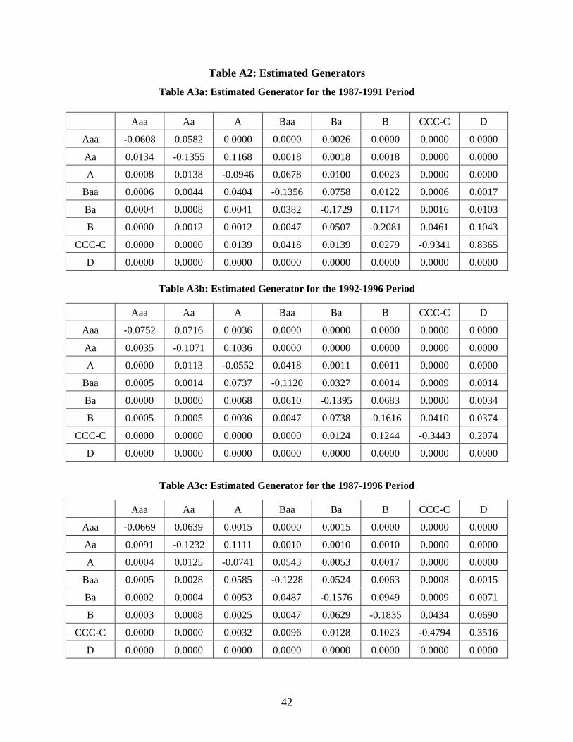
Table A2: Estimated Generators

Table A3a: Estimated Generator for the 1987-1991 Period

Aaa Aa A Baa Ba B CCC-C D

Aaa -0.0608 0.0582 0.0000 0.0000 0.0026 0.0000 0.0000 0.0000

Aa 0.0134 -0.1355 0.1168 0.0018 0.0018 0.0018 0.0000 0.0000

A 0.0008 0.0138 -0.0946 0.0678 0.0100 0.0023 0.0000 0.0000

Baa 0.0006 0.0044 0.0404 -0.1356 0.0758 0.0122 0.0006 0.0017

Ba 0.0004 0.0008 0.0041 0.0382 -0.1729 0.1174 0.0016 0.0103

B 0.0000 0.0012 0.0012 0.0047 0.0507 -0.2081 0.0461 0.1043

CCC-C 0.0000 0.0000 0.0139 0.0418 0.0139 0.0279 -0.9341 0.8365

D 0.0000 0.0000 0.0000 0.0000 0.0000 0.0000 0.0000 0.0000

Table A3b: Estimated Generator for the 1992-1996 Period

Aaa Aa A Baa Ba B CCC-C D

Aaa -0.0752 0.0716 0.0036 0.0000 0.0000 0.0000 0.0000 0.0000

Aa 0.0035 -0.1071 0.1036 0.0000 0.0000 0.0000 0.0000 0.0000

A 0.0000 0.0113 -0.0552 0.0418 0.0011 0.0011 0.0000 0.0000

Baa 0.0005 0.0014 0.0737 -0.1120 0.0327 0.0014 0.0009 0.0014

Ba 0.0000 0.0000 0.0068 0.0610 -0.1395 0.0683 0.0000 0.0034

B 0.0005 0.0005 0.0036 0.0047 0.0738 -0.1616 0.0410 0.0374

CCC-C 0.0000 0.0000 0.0000 0.0000 0.0124 0.1244 -0.3443 0.2074

D 0.0000 0.0000 0.0000 0.0000 0.0000 0.0000 0.0000 0.0000

Table A3c: Estimated Generator for the 1987-1996 Period

Aaa Aa A Baa Ba B CCC-C D

Aaa -0.0669 0.0639 0.0015 0.0000 0.0015 0.0000 0.0000 0.0000

Aa 0.0091 -0.1232 0.1111 0.0010 0.0010 0.0010 0.0000 0.0000

A 0.0004 0.0125 -0.0741 0.0543 0.0053 0.0017 0.0000 0.0000

Baa 0.0005 0.0028 0.0585 -0.1228 0.0524 0.0063 0.0008 0.0015

Ba 0.0002 0.0004 0.0053 0.0487 -0.1576 0.0949 0.0009 0.0071

B 0.0003 0.0008 0.0025 0.0047 0.0629 -0.1835 0.0434 0.0690

CCC-C 0.0000 0.0000 0.0032 0.0096 0.0128 0.1023 -0.4794 0.3516

D 0.0000 0.0000 0.0000 0.0000 0.0000 0.0000 0.0000 0.0000

42

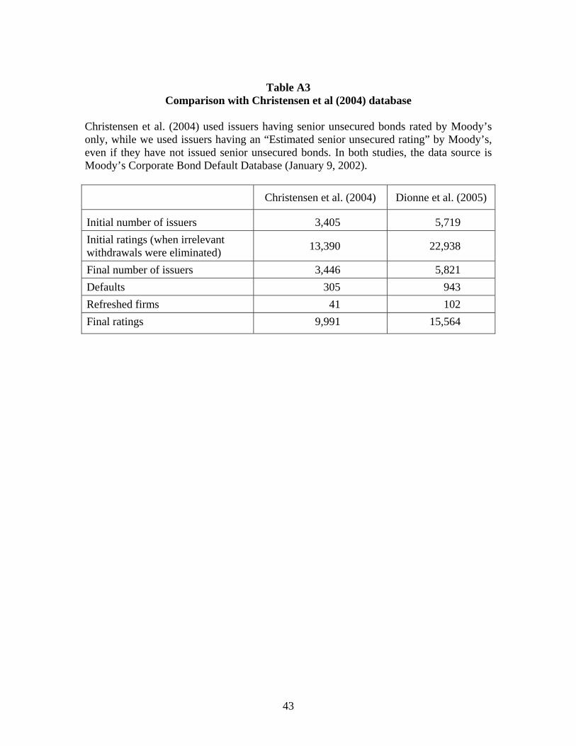
Table A3

Comparison with Christensen et al (2004) database

Christensen et al. (2004) used issuers having senior unsecured bonds rated by Moody’s only, while we used issuers having an “Estimated senior unsecured rating” by Moody’s, even if they have not issued senior unsecured bonds. In both studies, the data source is Moody’s Corporate Bond Default Database (January 9, 2002).

Christensen et al. (2004) Dionne et al. (2005)

Initial number of issuers 3,405 5,719 Initial ratings (when irrelevant withdrawals were eliminated) 13,390 22,938

Final number of issuers 3,446 5,821 Defaults 305 943 Refreshed firms 41 102 Final ratings 9,991 15,564

43

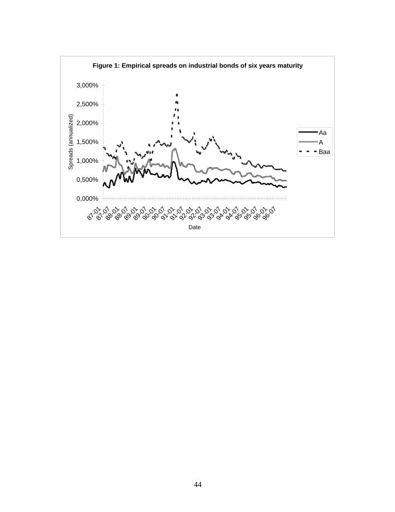
Figure 1: Empirical spreads on industrial bonds of six years maturity

0,000%

0,500%

1,000%

1,500%

2,000%

2,500%

3,000%

87-01

87-07

88-01

88-07

89-01

89-07

90-01

90-07

91-01

91-07

92-01

92-07

93-01

93-07

94-01

94-07

95-01

95-07

96-01

96-07

Date

Spr

eads

(ann

ualiz

ed)

AaABaa

44

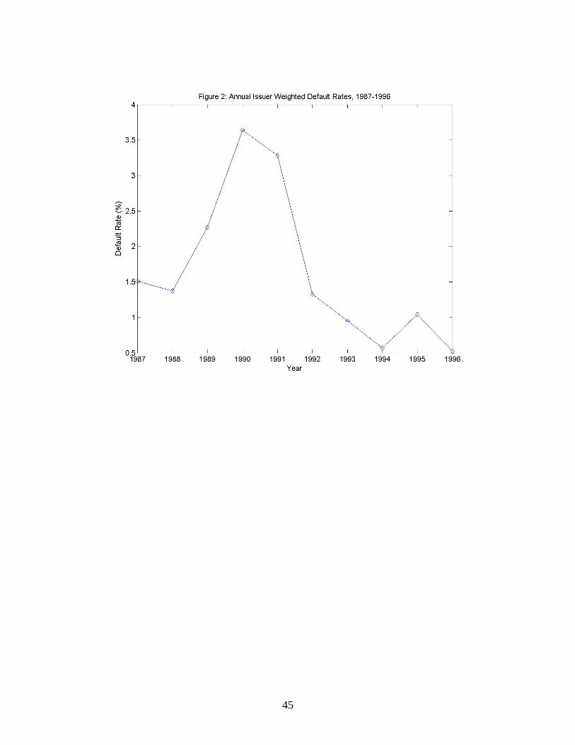
45

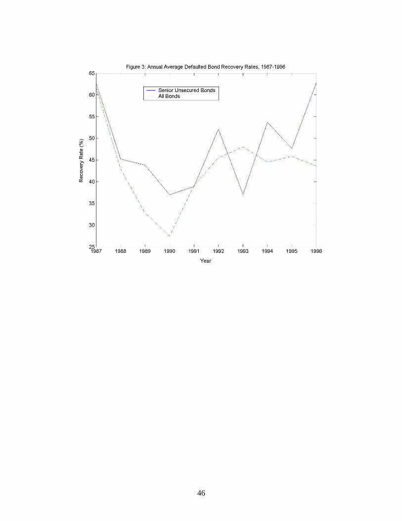
46