
Chapter 1 - LAMSADE - CNRS UMR 7243 - Université …bouyssou/conjoint.pdfnumbers attached to the...
64
Chapter 1 CONJOINT MEASUREMENT TOOLS FOR MCDM A brief introduction Denis Bouyssou CNRS LAMSADE, Universit´ e Paris Dauphine F-75775 Paris Cedex 16 France [email protected] Marc Pirlot Facult´ e Polytechnique de Mons 9, rue de Houdain B-7000 Mons Belgium [email protected] Abstract This paper offers a brief and nontechnical introduction to the use of con- joint measurement in multiple criteria decision making. The emphasis is on the, central, additive value function model. We outline its axiomatic foundations and present various possible assessment techniques to im- plement it. Some extensions of this model, e.g. nonadditive models or models tolerating intransitive preferences are then briefly reviewed. Keywords: Conjoint Measurement, Additive Value Function, Preference Modelling. 1. Introduction and motivation Conjoint measurement is a set of tools and results first developed in Eco- nomics [44] and Psychology [141] in the beginning of the ‘60s. Its, ambi- tious, aim is to provide measurement techniques that would be adapted 1
Transcript of Chapter 1 - LAMSADE - CNRS UMR 7243 - Université …bouyssou/conjoint.pdfnumbers attached to the...

Chapter 1
CONJOINT MEASUREMENT TOOLS FORMCDM
A brief introduction
Denis BouyssouCNRS
LAMSADE, Universite Paris Dauphine
F-75775 Paris Cedex 16
France
Marc PirlotFaculte Polytechnique de Mons
9, rue de Houdain
B-7000 Mons
Belgium
Abstract This paper offers a brief and nontechnical introduction to the use of con-joint measurement in multiple criteria decision making. The emphasis ison the, central, additive value function model. We outline its axiomaticfoundations and present various possible assessment techniques to im-plement it. Some extensions of this model, e.g. nonadditive models ormodels tolerating intransitive preferences are then briefly reviewed.
Keywords: Conjoint Measurement, Additive Value Function, Preference Modelling.
1. Introduction and motivation
Conjoint measurement is a set of tools and results first developed in Eco-nomics [44] and Psychology [141] in the beginning of the ‘60s. Its, ambi-tious, aim is to provide measurement techniques that would be adapted
1
2
to the needs of the Social Sciences in which, most often, multiple dimen-sions have to be taken into account.
Soon after its development, people working in decision analysis real-ized that the techniques of conjoint measurement could also be used astools to structure preferences [51, 165]. This is the subject of this paperwhich offers a brief and nontechnical introduction to conjoint measure-ment models and their use in multiple criteria decision making. Moredetailed treatments may be found in [63, 79, 121, 135, 209]. Advancedreferences include [58, 129, 211].
1.1. Conjoint measurement models in decisiontheory
The starting point of most works in decision theory is a binary relation% on a set A of objects. This binary relation is usually interpreted asan “at least as good as” relation between alternative courses of actiongathered in A.
Manipulating a binary relation can be quite cumbersome as soon asthe set of objects is large. Therefore, it is not surprising that manyworks have looked for a numerical representation of the binary relation%. The most obvious numerical representation amounts to associate areal number V (a) to each object a ∈ A in such a way that the comparisonbetween these numbers faithfully reflects the original relation %. Thisleads to defining a real-valued function V on A, such that:
a % b ⇔ V (a) ≥ V (b), (1.1)
for all a, b ∈ A. When such a numerical representation is possible, onecan use V instead of % and, e.g. apply classical optimization techniquesto find the most preferred elements in A given %. We shall call such afunction V a value function.
It should be clear that not all binary relations % may be representedby a value function. Condition (1.1) imposes that % is complete (i.e.a % b or b % a, for all a, b ∈ A) and transitive (i.e. a % b and b % cimply a % c, for all a, b, c ∈ A). When A is finite or countably infinite,it is well-known [58, 129] that these two conditions are, in fact, not onlynecessary but also sufficient to build a value function satisfying (1.1).
Remark 1The general case is more complex since (1.1) implies, for instance, thatthere must be “enough” real numbers to distinguish objects that have tobe distinguished. The necessary and sufficient conditions for (1.1) can befound in [58, 129]. An advanced treatment is [13]. Sufficient conditions
An introduction to conjoint measurement 3
that are well-adapted to cases frequently encountered in Economics canbe found in [42, 45]; see [34] for a synthesis. •
It is vital to note that, when a value function satisfying (1.1) exists, it isby no means unique. Taking any increasing function φ on R, it is clearthat φ◦V gives another acceptable value function. A moment of reflectionwill convince the reader that only such transformations are acceptableand that if V and U are two real-valued functions on A satisfying (1.1),they must be related by an increasing transformation. In other words, avalue function in the sense of (1.1) defines an ordinal scale.
Ordinal scales, although useful, do not allow the use of sophisticatedassessment procedures, i.e. of procedures that allow an analyst to assessthe relation % through a structured dialogue with the decision-maker.This is because the knowledge that V (a) ≥ V (b) is strictly equivalent tothe knowledge of a % b and no inference can be drawn from this assertionbesides the use of transitivity.
It is therefore not surprising that much attention has been devotedto numerical representations leading to more constrained scales. Manypossible avenues have been explored to do so. Among the most well-known, let us mention:
the possibility to compare probability distributions on the set A[58, 207]. If it is required that, not only (1.1) holds but that thenumbers attached to the objects should be such that their expectedvalues reflect the comparison of probability distributions on theset of objects, a much more constrained numerical representationclearly obtains,
the introduction of “preference difference” comparisons of the type:the difference between a and b is larger than the difference betweenc and d, see [44, 81, 123, 129, 159, 180, 199]. If it is required that,not only (1.1) holds, but that the differences between numbersalso reflect the comparisons of preference differences, a more con-strained numerical representation obtains.
When objects are evaluated according to several dimensions, i.e. when% is defined on a product set, new possibilities emerge to obtain numer-ical representations that would specialize (1.1). The purpose of conjointmeasurement is to study such kinds of models.
There are many situations in decision theory which call for the studyof binary relations defined on product sets. Among them let us mention:
Multiple criteria decision making using a preference relation com-paring alternatives evaluated on several attributes [16, 121, 162,173, 209],
4
Decision under uncertainty using a preference relation comparingalternatives evaluated on several states of nature [68, 107, 177, 184,210, 211],
Consumer theory manipulating preference relations for bundles ofseveral goods [43],
Intertemporal decision making using a preference relation betweenalternatives evaluated at several moments in time [121, 125, 126],
Inequality measurement comparing distributions of wealth acrossseveral individuals [5, 17, 18, 217].
The purpose of this paper is to give an introduction to the main modelsof conjoint measurement useful in multiple criteria decision making. Theresults and concepts that are presented may however be of interest in allof the afore-mentioned areas of research.
Remark 2Restricting ourselves to applications in multiple criteria decision makingwill not allow us to cover every aspect of conjoint measurement. Amongthe most important topics left aside, let us mention: the introduction ofstatistical elements in conjoint measurement models [54, 108] and thetest of conjoint measurement models in experiments [135]. •
Given a binary relation % on a product set X = X1 ×X2 × · · · ×Xn,the theory of conjoint measurement consists in finding conditions underwhich it is possible to build a convenient numerical representation of %and to study the uniqueness of this representation. The central modelis the additive value function model in which:
x % y ⇔n
∑
i=1
vi(xi) ≥n
∑
i=1
vi(yi) (1.2)
where vi are real-valued functions, called partial value functions, onthe sets Xi and it is understood that x = (x1, x2, . . . , xn) and y =(y1, y2, . . . , yn). Clearly if % has a representation in model (1.2), takingany common increasing transformation of the vi will not lead to anotherrepresentation in model (1.2).
Specializations of this model in the above-mentioned areas give severalcentral models in decision theory:
The Subjective Expected Utility model, in the case of decision-making under uncertainty,
The discounted utility model for dynamic decision making,
An introduction to conjoint measurement 5
Inequality measures a la Atkinson/Sen in the area of social welfare.
The axiomatic analysis of this model is now quite firmly established[44, 129, 211]; this model forms the basis of many decision analysis tech-niques [79, 121, 209, 211]. This is studied in sections 3 and 4 after weintroduce our main notation and definitions in section 2.
Remark 3One possible objection to the study of model (1.2) is that the choice ofan additive model seems arbitrary and restrictive. It should be observedhere that the functions vi will precisely be assessed so that additivityholds. Furthermore, the use of a simple model may be seen as an advan-tage in view of the limitations of the cognitive abilities of most humanbeings.
It is also useful to notice that this model can be reformulated so asto make addition disappear. Indeed if there are partial value functionsvi such that (1.2) holds, it is clear that V =
∑ni=1 vi is a value function
satisfying (1.1). Since V defines an ordinal scale, taking the exponentialof V leads to another valid value function W . Clearly W has now amultiplicative form:
x % y ⇔ W (x) =n
∏
i=1
wi(xi) ≥ W (y) =n
∏
i=1
wi(yi).
where wi(xi) = evi(xi).The reader is referred to chapter XXX (Chapter 6, Dyer) for the
study of situations in which V defines a scale that is more constrainedthan an ordinal scale, e.g. because it is supposed to reflect preferencedifferences or because it allows to compute expected utilities. In suchcases, the additive form (1.2) is no more equivalent to the multiplicativeform considered above. •
In section 5 we present a number of extensions of this model going fromnonadditive representations of transitive relations to model toleratingintransitive indifference and, finally, nonadditive representations of non-transitive relations.
Remark 4In this paper, we shall restrict our attention to the case in which alter-natives may be evaluated on the various attributes without risk or un-certainty. Excellent overviews of these cases may be found in [121, 209];recent references include [142, 150]. •
Before starting our study of conjoint measurement oriented towardsMCDM, it is worth recalling that conjoint measurement aims at estab-lishing measurement models in the Social Sciences. To many, the very
6
notion of “measurement in the Social Sciences” may appear contradic-tory. It may therefore be useful to briefly consider how the notion ofmeasurement can be modelled in Physics, an area in which the notionof “measurement” seems to arise quite naturally, and to explain how a“measurement model” may indeed be useful in order to structure pref-erences.
1.2. An aside: measuring length
Physicists usually take measurement for granted and are not particularlyconcerned with the technical and philosophical issues it raises (at leastwhen they work within the realm of Newtonian Physics). However, fora Social Scientist, these question are of utmost importance. It may thushelp to have an idea of how things appear to work in Physics beforetackling more delicate cases.
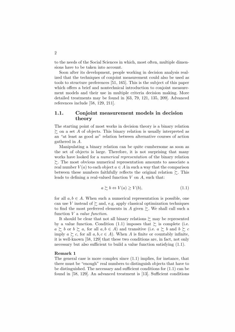
Suppose that you are on a desert island and that you want to “mea-sure” the length of a collection of rigid straight rods. Note that we do notdiscuss here the “pre-theoretical” intuition that “length” is a propertyof these rods that can be measured, as opposed, say, to their softness ortheir beauty.
r r′
r  r′s s′
s ∼ s′
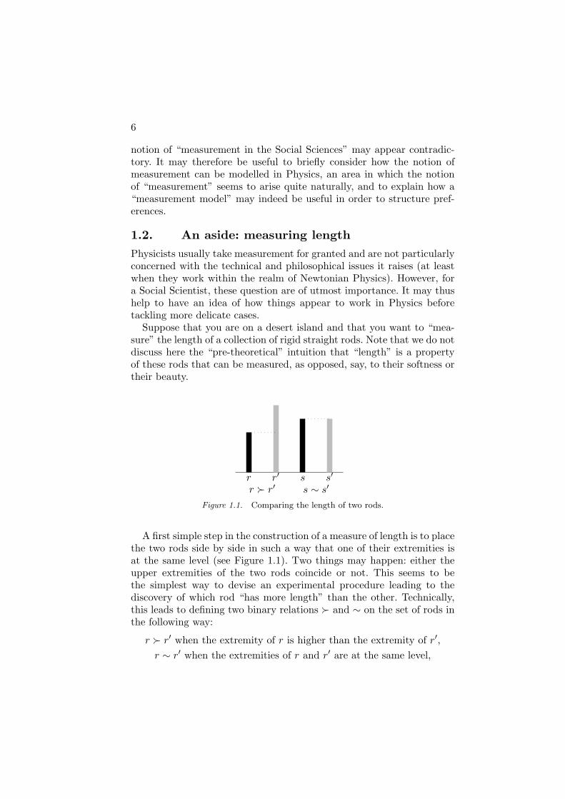
Figure 1.1. Comparing the length of two rods.
A first simple step in the construction of a measure of length is to placethe two rods side by side in such a way that one of their extremities isat the same level (see Figure 1.1). Two things may happen: either theupper extremities of the two rods coincide or not. This seems to bethe simplest way to devise an experimental procedure leading to thediscovery of which rod “has more length” than the other. Technically,this leads to defining two binary relations  and ∼ on the set of rods inthe following way:
r  r′ when the extremity of r is higher than the extremity of r′,
r ∼ r′ when the extremities of r and r′ are at the same level,
An introduction to conjoint measurement 7
Clearly, if length is a quality of the rods that can be measured, it isexpected that these pairwise comparisons are somehow consistent, e.g.,
if r  r′ and r′  r′′, it should follow that r  r′′,
if r ∼ r′ and r′ ∼ r′′, it should follow that r ∼ r′′,
if r ∼ r′ and r′  r′′, it should follow that r  r′′.
Although quite obvious, these consistency requirements are stringent.For instance, the second and the third conditions are likely to be violatedif the experimental procedure involves some imprecision, e.g if two rodsthat slightly differ in length are nevertheless judged “equally long”. Theyrepresent a form of idealization of what could be a perfect experimentalprocedure.
With the binary relations  and ∼ at hand, we are still rather farfrom a full-blown measure of length. It is nevertheless possible to as-sign numbers to each of the rods in such a way that the comparisonof these numbers reflects what has been obtained experimentally. Whenthe consistency requirements mentioned above are satisfied, it is indeedgenerally possible to build a real-valued function Φ on the set of rodsthat would satisfy:
r  r′ ⇔ Φ(r) > Φ(r′) and
r ∼ r′ ⇔ Φ(r) = Φ(r′).
If the experiment is costly or difficult to perform, such a numerical as-signment may indeed be useful because it summarizes, once for all, whathas been obtained in experiments. Clearly there are many possible waysto assign numbers to rods in this way. Up to this point, they are equallygood for our purposes. The reader will easily check that defining % as or ∼, the function Φ is noting else than a “value function” for length:any increasing transformation may therefore be applied to Φ.
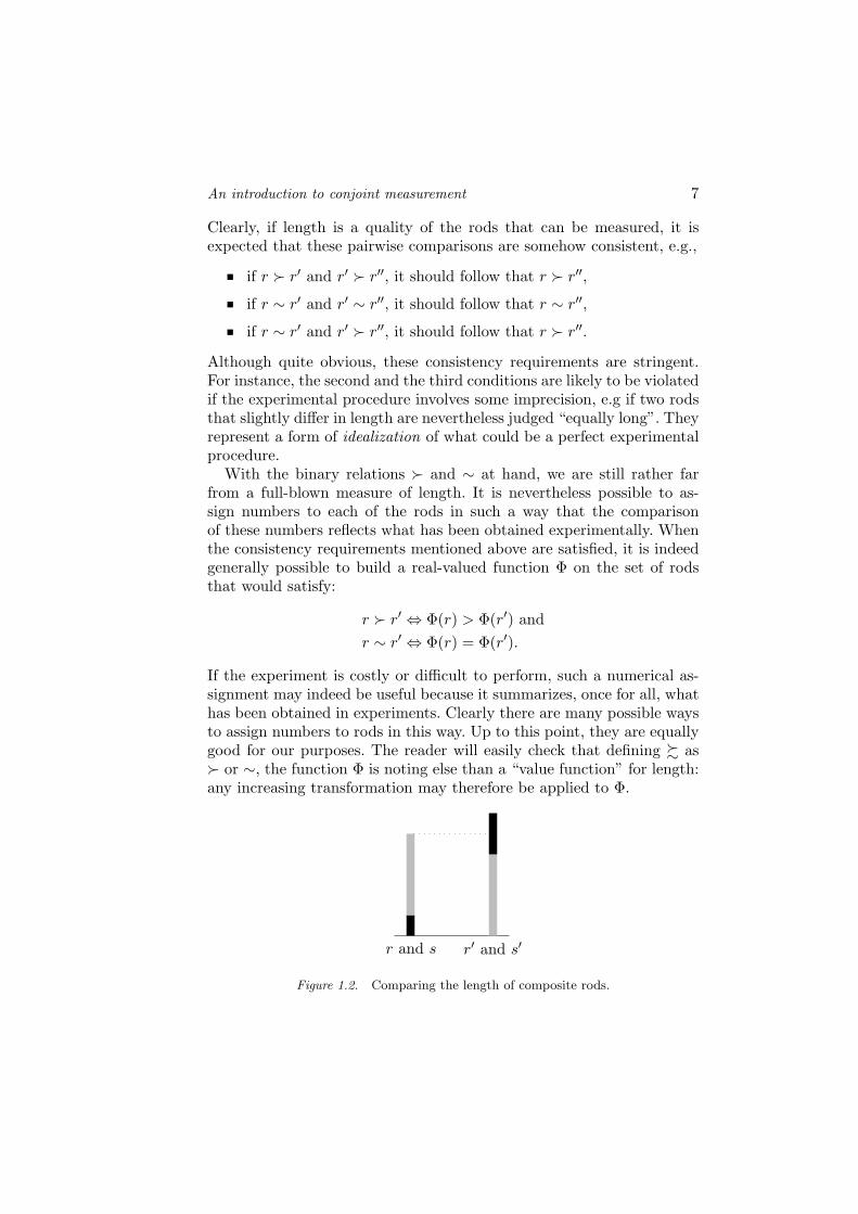
r and s r′ and s′
Figure 1.2. Comparing the length of composite rods.

8
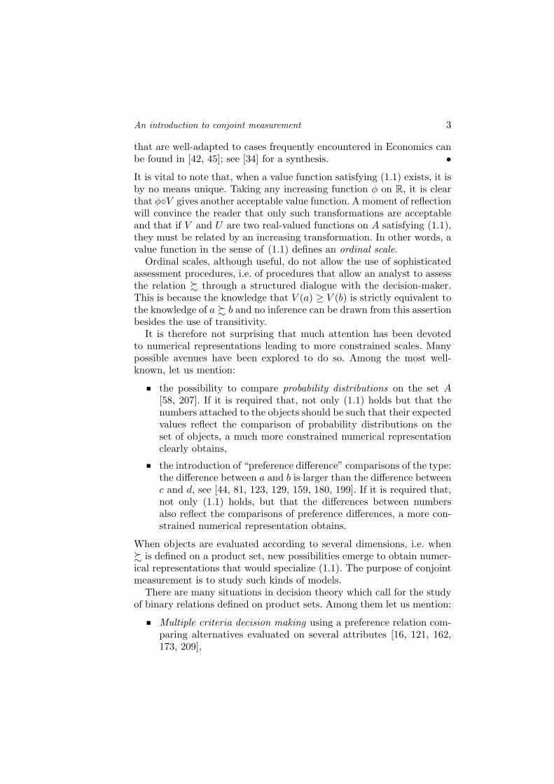
The next major step towards the construction of a measure of lengthis the realization that it is possible to form new rods by simply placingtwo or more rods “in a row”, i.e. you may concatenate rods. From thepoint of view of length, it seems obvious to expect this concatenationoperation ◦ to be “commutative” (r ◦ s has the same length as s◦ r) andassociative ((r ◦ s) ◦ t has the same length as r ◦ (s ◦ t)).
You clearly want to be able to measure the length of these compositeobjects and you can always include them in our experimental procedureoutlined above (see Figure 1.2). Ideally, you would like your numericalassignment Φ to be somehow compatible with the concatenation oper-ation: knowing the numbers assigned to two rods, you want to be ableto deduce the number assigned to their concatenation. The most ob-vious way to achieve that is to require that the numerical assignmentof a composite object can be deduced by addition from the numericalassignments of the objects composing it, i.e. that
Φ(r ◦ r′) = Φ(r) + Φ(r′).
This clearly places many additional constraints on the results of yourexperiment. An obvious one is that  and ∼ should be compatible withthe concatenation operation ◦, e.g.
r  r′ and t ∼ t′ should lead to r ◦ t  r′ ◦ t′.
These new constraints may or may not be satisfied. When they are,the usefulness of the numerical assignment Φ is even more apparent: asimple arithmetic operation will allow to infer the result of an experimentinvolving composite objects.
Let us take a simple example. Suppose that you have 5 rods r1, r2, . . . , r5
and that, because space is limited, you can only concatenate at most tworods and that not all concatenations are possible. Let us suppose, for themoment, that you do not have much technology available so that youmay only experiment using different rods. You may well collect the fol-lowing information, using obvious notation exploiting the transitivity of which holds in this experiment,
r1 ◦ r5 Â r3 ◦ r4 Â r1 ◦ r2 Â r5 Â r4 Â r3 Â r2 Â r1.
Your problem is then to find a numerical assignment Φ to rods such thatusing an addition operation, you can infer the numerical assignment ofcomposite objects consistently with your observations. Let us considerthe following three assignments:
An introduction to conjoint measurement 9
Φ Φ′ Φ′′
r1 14 10 14r2 15 91 16r3 20 92 17r4 21 93 18r5 28 100 29
These three assignments are equally valid to reflect the comparisons ofsingle rods. Only the first and the third allow to capture the comparisonsof composite objects that were performed. Note that, going from Φ to Φ′′
does not involve just changing the “unit of measurement”: since Φ(r1) =Φ′′(r1) this would imply that Φ = Φ′′, which is clearly false.
Such numerical assignments have limited usefulness. Indeed, it is tempt-ing to use them to predict the result of comparisons that we have notbeen able to perform. But this turns out to be quite disappointing: usingΦ you would conclude that r2◦r3 ∼ r1◦r4 since Φ(r2)+Φ(r3) = 15+20 =35 = Φ(r1)+Φ(r4), but, using Φ′′, you would conclude that r2◦r3 Â r1◦r4
since Φ′′(r2)+Φ′′(r3) = 16+17 = 33 while Φ′′(r1)+Φ′′(r4) = 14+18 = 32.Intuitively, “measuring” calls for some kind of a standard (e.g. the
“Metre-etalon” that can be found in the Bureau International des Poidset Mesures in Sevres, near Paris). This implies choosing an appropriate“standard” rod and being able to prepare perfect copies of this standardrod (we say here “appropriate” because the choice of a standard shouldbe made in accordance with the lengths of the objects to be measured:a tiny or a huge standard will not facilitate experiments). Let us call s0
the standard rod. Let us suppose that you have been able to prepare alarge number of perfect copies s1, s2, . . . of s0. We therefore have:
s0 ∼ s1, s0 ∼ s2, s0 ∼ s3, . . .
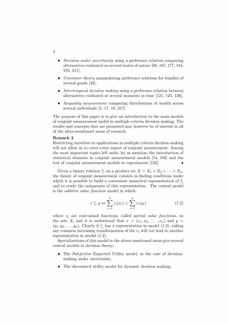
Let us also agree that the length of s0 is 1. This is your, arbitrary,unit of length. How can you use s0 and its perfect copies so as to de-termine unambiguously the length of any other (simple or composite)object? Quite simply, you may prepare a “standard sequence of lengthn”, S(n) = s1 ◦s2 ◦ . . .◦sn−1 ◦sn, i.e. a composite object that is made byconcatenating n perfect copies of our standard rod s0. The length of astandard sequence of length n is exactly n since we have concatenated nobjects that are perfect copies of the standard rod of length 1. Take anyrod r and let us compare r with several standard sequences of increasinglength: S(1), S(2), . . .
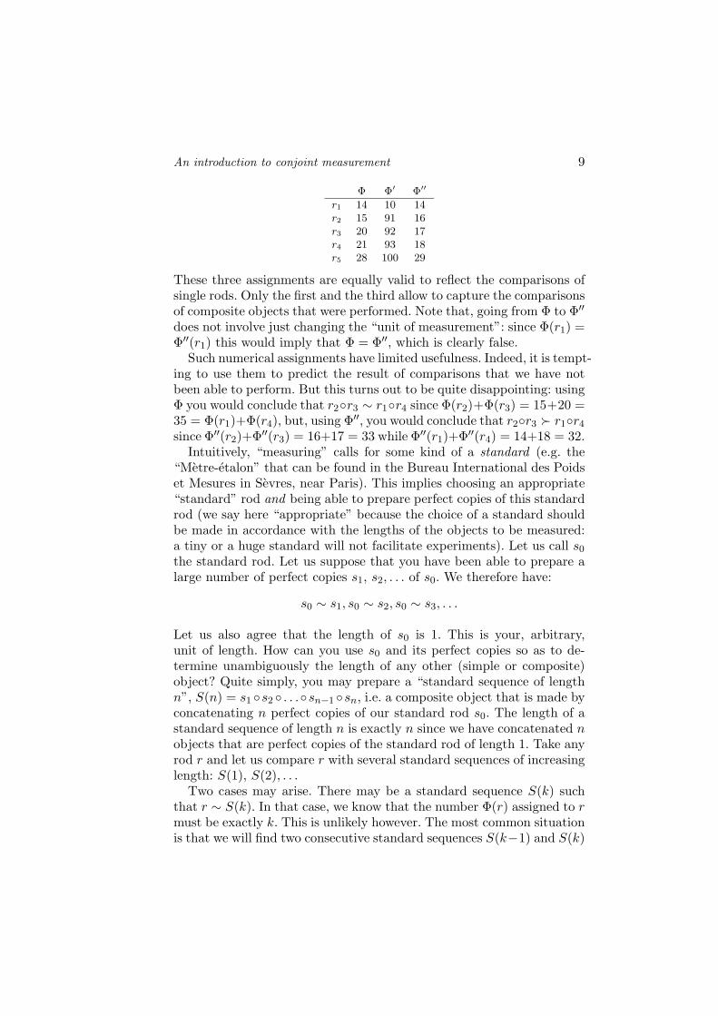
Two cases may arise. There may be a standard sequence S(k) suchthat r ∼ S(k). In that case, we know that the number Φ(r) assigned to rmust be exactly k. This is unlikely however. The most common situationis that we will find two consecutive standard sequences S(k−1) and S(k)
10
such that r  S(k − 1) and S(k)  r (see Figure 1.3). This means thatΦ(r) must be such that k−1 < Φ(r) < k. We seem to be in trouble heresince, as before, Φ(r) is not exactly determined. How can you proceed?This depends on your technology for preparing perfect copies.
r S(k)
s1
s2
s3
s4
s5
s6
s7
s8
r  S(7), S(8)  r
7 < Φ(r) < 8
Figure 1.3. Using standard sequences.
Imagine that you are able to prepare perfect copies not only of thestandard rod but also of any object. You may then prepare several copies(r1, r2, . . .) of the rod r. You can now compare a composite object madeout of two perfect copies of r with your standard sequences S(1), S(2), . . .As before, you shall eventually arrive at locating Φ(r1 ◦ r2) = 2Φ(r)within an interval of width 1. This means that the interval of impre-cision surrounding Φ(r) has been divided by two. Continuing this pro-cess, considering longer and longer sequences of perfect copies of r, youwill keep on reducing the width of the interval containing Φ(r). Thismeans that you can approximate Φ(r) with any given level of precision.Mathematically, a unique value for Φ(r) will be obtained using a simpleargument.
Supposing that you are in position to prepare perfect copies of anyobject is a strong technological requirement. When this is not possible,there still exists a way out. Instead of preparing a perfect copy of ryou may also try to increase the granularity of your standard sequence.This means building an object t that you would be able to replicateperfectly and such that concatenating t with one of its perfect replicasgives an object that has exactly the length of the standard object s0, i.e.Φ(t) = 1/2. Considering standard sequences based on t, you will be ableto increase by a factor 2 the precision with which we measure the lengthof r. Repeating the process, i.e. subdividing t, will lead, as before, to aunique limiting value for Φ(r).
An introduction to conjoint measurement 11
The mathematical machinery underlying the measurement process in-formally described above (called “extensive measurement”) rests on thetheory of ordered groups. It is beautifully described and illustrated in[129]. Although the underlying principles are simple, we may expect com-plications to occur e.g. when not all concatenations are feasible, whenthere is some level (say the velocity of light if we were to measure speed)that cannot be exceeded or when it comes to relate different measures.See [129, 140, 168] for a detailed treatment.
Clearly, this was an overly detailed and unnecessary complicated de-scription of how length could be measured. Since our aim is to eventuallydeal with “measurement” in the Social Sciences, it may however be usefulto keep the above process in mind. Its basic ingredients are the following:
well-behaved relations  and ∼ allowing to compare objects,
a concatenation operation ◦ allowing to consider composite ob-jects,
consistency requirements linking Â, ∼ and ◦,
the ability to prepare perfect copies of some objects in order tobuild standard sequences.
Basically, conjoint measurement is a quite ingenious way to performrelated measurement operations when no concatenation operation isavailable. This will however require that objects can be evaluated alongseveral dimensions. Before explaining how this might work, it is worthexplaining the context in which such measurement might prove useful.
Remark 5It is often asserted that “measurement is impossible in the Social Sci-ences” precisely because the Social Scientist has no way to define a con-catenation operation. Indeed, it would seem hazardous to try to con-catenate the intelligence of two subjects or the pain of two patients (see[56, 106]). Under certain conditions, the power of conjoint measurementwill precisely be to provide a means to bypass this absence of read-ily available concatenation operation when the objects are evaluated onseveral dimensions.
Let us remark that, even when there seems to be a concatenation op-eration readily available, it does not always fit the purposes of extensivemeasurement. Consider for instance an individual expressing preferencesfor the quantity of the two goods he consumes. The objects therefore takethe well structured form of points in the positive orthant of R
2. Thereseems to be an obvious concatenation operation here: (x, y)◦(z, w) mightsimply be taken to be (x + y, z + w). However a fairly rational person,
12
consuming pants and jackets, may indeed prefer (3, 0) (3 pants and nojacket) to (0, 3) (no pants and 3 jackets) but at the same time prefer(3, 3) to (6, 0). This implies that these preferences cannot be explainedby a measure that would be additive with respect to the concatena-tion operation consisting in adding the quantities of the two goods con-sumed. Indeed (3, 0) Â (0, 3) implies Φ(3, 0) > Φ(0, 3), which impliesΦ(3, 0) + Φ(3, 0) > Φ(0, 3) + Φ(3, 0). Additivity with respect to con-catenation should then imply that (3, 0) ◦ (3, 0) Â (0, 3) ◦ (3, 0), that is(6, 0) Â (3, 3).
1.3. An example: Even swaps
The even swaps technique described and advocated in [120, 121, 165] isa simple way to deal with decision problems involving several attributesthat does not have recourse to a formal representation of preferences,which will be the subject of conjoint measurement. Because this tech-nique is simple and may be quite useful, we describe it below using thesame example as in [120]. This will also allow to illustrate the type ofproblems that are dealt with in decision analysis applications of conjointmeasurement.
Example 6 (Even swaps technique)A consultant considers renting a new office. Five different locations havebeen identified after a careful consideration of many possibilities, reject-ing all those that do not meet a number of requirements.
His feeling is that five distinct characteristics, we shall say five at-tributes, of the possible locations should enter into his decision: his dailycommute time (expressed in minutes), the ease of access for his clients(expressed as the percentage of his present clients living close to the of-fice), the level of services offered by the new office (expressed on an adhoc scale with three levels: A (all facilities available), B (telephone andfax), C (no facilities)), the size of the office expressed in square feet, andthe monthly cost expressed in dollars.
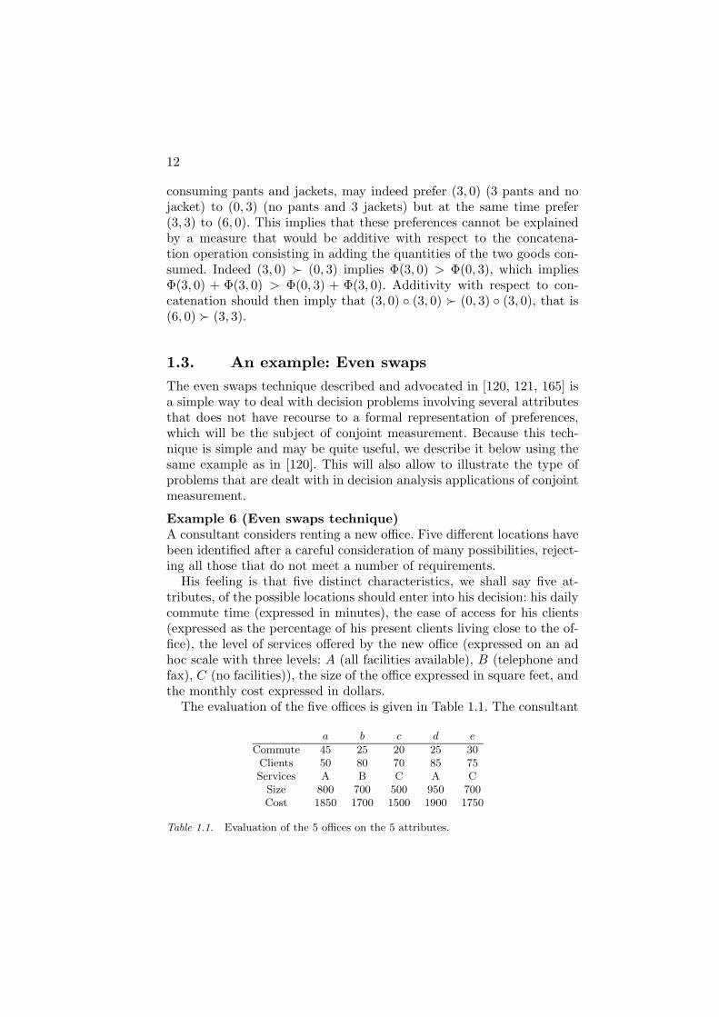
The evaluation of the five offices is given in Table 1.1. The consultant
a b c d e
Commute 45 25 20 25 30Clients 50 80 70 85 75Services A B C A C
Size 800 700 500 950 700Cost 1850 1700 1500 1900 1750
Table 1.1. Evaluation of the 5 offices on the 5 attributes.

An introduction to conjoint measurement 13
has well-defined preferences on each of these attributes, independentlyof what is happening on the other attributes. His preference increaseswith the level of access for his clients, the level of services of the officeand its size. It decreases with commute time and cost. This gives a firsteasy way to compare alternatives through the use of dominance.
An alternative y is dominated by an alternative x if x is at least asgood as y on all attributes while being strictly better for at least oneattribute. Clearly dominated alternatives are not candidate for the finalchoice and may, thus, be dropped from consideration. The reader willeasily check that, on this example, alternative b dominates alternative e:e and b have similar size but b is less expensive, involves a shorter com-mute time, an easier access to clients and a better level of services. Wemay therefore forget about alternative e. This is the only case of “puredominance” in our table. It is however easy to see that d is “close” todominating a, the only difference in favor of a being on the cost attribute(50 $ per month). This is felt more than compensated by the differencesin favor of d on all other attributes: commute time (20 minutes), clientaccess (35 %) and size (150 sq. feet).
Dropping all alternatives that are not candidate for choice, this initialinvestigation allows to reduce the problem to:
b c d
Commute 25 20 25Clients 80 70 85Services B C A
Size 700 500 950Cost 1700 1500 1900
A natural way to proceed is then to assess tradeoffs. Observe that allalternatives but c have a common evaluation on commute time. We maytherefore ask the consultant, starting with office c, what gain on clientaccess would compensate a loss of 5 minutes on commute time. We arelooking for an alternative c′ that would be evaluated as follows:
c c′
Commute 20 25
Clients 70 70 + δ
Services C C
Size 500 500Cost 1500 1500
and judged indifferent to c. Although this is not an easy question, it isclearly crucial in order to structure preferences.
Remark 7In this paper, we do not consider the possibility of lexicographic pref-erences, in which such tradeoffs do not occur, see [59, 60, 160]. Lexico-
14
graphic preferences may also be combined with the possibility of “local”tradeoffs, see [22, 64, 136]. •
Remark 8Since tradeoffs questions may be difficult, it is wise to start with anattribute requiring few assessments (in the example, all alternatives butone have a common evaluation on commute time). Clearly this attributeshould be traded against one with an underlying “continuous” structure(cost, in the example). •
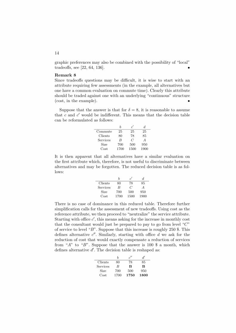
Suppose that the answer is that for δ = 8, it is reasonable to assumethat c and c′ would be indifferent. This means that the decision tablecan be reformulated as follows:
b c′ d
Commute 25 25 25Clients 80 78 85Services B C A
Size 700 500 950Cost 1700 1500 1900
It is then apparent that all alternatives have a similar evaluation onthe first attribute which, therefore, is not useful to discriminate betweenalternatives and may be forgotten. The reduced decision table is as fol-lows:
b c′ d
Clients 80 78 85Services B C A
Size 700 500 950Cost 1700 1500 1900
There is no case of dominance in this reduced table. Therefore furthersimplification calls for the assessment of new tradeoffs. Using cost as thereference attribute, we then proceed to “neutralize” the service attribute.Starting with office c′, this means asking for the increase in monthly costthat the consultant would just be prepared to pay to go from level “C”of service to level “B”. Suppose that this increase is roughly 250 $. Thisdefines alternative c′′. Similarly, starting with office d we ask for thereduction of cost that would exactly compensate a reduction of servicesfrom “A” to “B”. Suppose that the answer is 100 $ a month, whichdefines alternative d′. The decision table is reshaped as:
b c′′ d′
Clients 80 78 85Services B B B
Size 700 500 950Cost 1700 1750 1800
An introduction to conjoint measurement 15
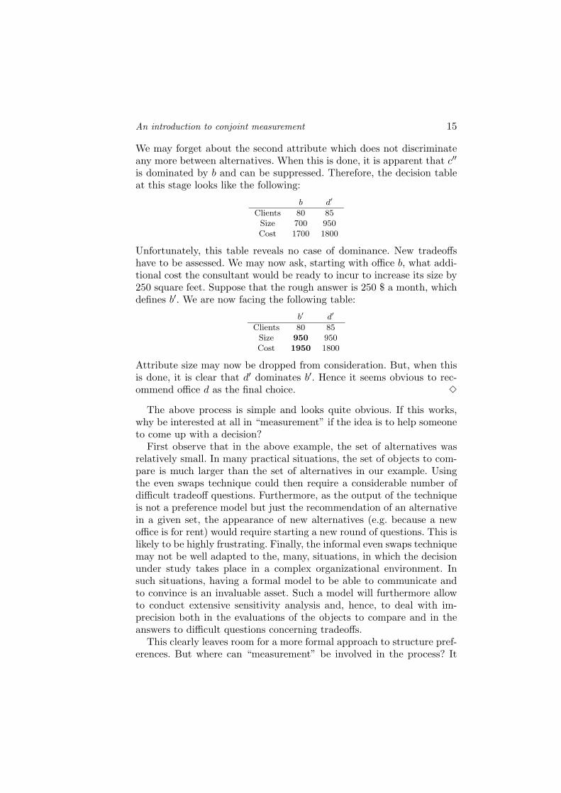
We may forget about the second attribute which does not discriminateany more between alternatives. When this is done, it is apparent that c′′
is dominated by b and can be suppressed. Therefore, the decision tableat this stage looks like the following:
b d′
Clients 80 85Size 700 950Cost 1700 1800
Unfortunately, this table reveals no case of dominance. New tradeoffshave to be assessed. We may now ask, starting with office b, what addi-tional cost the consultant would be ready to incur to increase its size by250 square feet. Suppose that the rough answer is 250 $ a month, whichdefines b′. We are now facing the following table:
b′ d′
Clients 80 85Size 950 950Cost 1950 1800
Attribute size may now be dropped from consideration. But, when thisis done, it is clear that d′ dominates b′. Hence it seems obvious to rec-ommend office d as the final choice. 3
The above process is simple and looks quite obvious. If this works,why be interested at all in “measurement” if the idea is to help someoneto come up with a decision?
First observe that in the above example, the set of alternatives wasrelatively small. In many practical situations, the set of objects to com-pare is much larger than the set of alternatives in our example. Usingthe even swaps technique could then require a considerable number ofdifficult tradeoff questions. Furthermore, as the output of the techniqueis not a preference model but just the recommendation of an alternativein a given set, the appearance of new alternatives (e.g. because a newoffice is for rent) would require starting a new round of questions. This islikely to be highly frustrating. Finally, the informal even swaps techniquemay not be well adapted to the, many, situations, in which the decisionunder study takes place in a complex organizational environment. Insuch situations, having a formal model to be able to communicate andto convince is an invaluable asset. Such a model will furthermore allowto conduct extensive sensitivity analysis and, hence, to deal with im-precision both in the evaluations of the objects to compare and in theanswers to difficult questions concerning tradeoffs.
This clearly leaves room for a more formal approach to structure pref-erences. But where can “measurement” be involved in the process? It
16
should be observed that, beyond surface, there are many analogies be-tween the even swaps process and the measurement of length consideredabove.
First, note that, in both cases, objects are compared using binaryrelations. In the measurement of length, the binary relation  reads“is longer than”. Here it reads “is preferred to”. Similarly, the relation∼ reading before “has equal length” now reads “is indifferent to”. Wesupposed in the measurement of length process that  and ∼ wouldnicely combine in experiments: if r  r′ and r′ ∼ r′′ then we shouldobserve that r  r′′. Implicitly, a similar hypothesis was made in the evenswaps technique. To realize that this is the case, it is worth summarizingthe main steps of the argument.
We started with Table 1.1. Our overall recommendation was to rentoffice d. This means that we have reasons to believe that d is preferredto all other potential locations, i.e. d  a, d  b, d  c, and d  e. Howdid we arrive logically at such a conclusion?
Based on the initial table, using dominance and quasi-dominance, weconcluded that b was preferable to e and that d was preferable to a. Usingsymbols, we have b  e and d  a. After assessing some tradeoffs, weconcluded, using dominance, that b  c′′. But remember, c′′ was built soas to be indifferent to c′ and, in turn, c′ was built so as to be indifferentto c. That is, we have c′′ ∼ c′ and c′ ∼ c. Later, we built an alternative d′
that is indifferent to d (d ∼ d′) and an alternative b′ that is indifferent tob (b ∼ b′). We then concluded, using dominance, that d′ was preferableto b′ (d′ Â b′). Hence, we know that:
d  a, b  e,
c′′ ∼ c′, c′ ∼ c, b  c′′,
d ∼ d′, b ∼ b′, d′ Â b′.
Using the consistency rules linking  and ∼ that we considered for themeasurement of length, it is easy to see that the last line implies d  b.Since b  e, this implies d  e. It remains to show that d  c. But thesecond line leads to, combining  and ∼, b  c. Therefore d  b leadsto d  c and we are home. Hence, we have used the same propertiesfor preference and indifference as the properties of “is longer than” and“has equal length” that we hypothesized in the measurement of length.
Second it should be observed that expressing tradeoffs leads, indi-rectly, to equating the “length” of “preference intervals” on differentattributes. Indeed, remember how c′ was constructed above: saying thatc and c′ are indifferent more or less amounts to saying that the interval[25, 20] on commute time has exactly the same “length” as the interval[70, 78] on client access. Consider an alternative f that would be iden-
An introduction to conjoint measurement 17
tical to c except that it has a client access at 78%. We may again askwhich increase in client access would compensate a loss of 5 minutes oncommute time. In a tabular form we are now comparing the followingtwo alternatives:
f f ′
Commute 20 25Clients 78 78 + δ
Services C CSize 500 500Cost 1500 1500
Suppose that the answer is that for δ = 10, f and f ′ would be indiffer-ent. This means that the interval [25, 20] on commute time has exactlythe same length as the interval [78, 88] on client access. Now, we knowthat the preference intervals [70, 78] and [78, 88] have the same “length”.Hence, tradeoffs provide a means to equate two preference intervals onthe same attribute. This brings us quite close to the construction ofstandard sequences. This, we shall shortly do.
How does this information about the “length” of preference intervalsrelate to judgements of preference or indifference? Exactly as in theeven swaps technique. You can use this measure of “length” modifyingalternatives in such a way that they only differ on a single attribute andthen use a simple dominance argument.
Conjoint measurement techniques may roughly be seen as a formal-ization of the even swaps technique that leads to building a numericalmodel of preferences much in the same way that we built a numeri-cal model for length. This will require assessment procedures that willrest on the same principles as the standard sequence technique used forlength. This process of “measuring preferences” is not an easy one. Itwill however lead to a numerical model of preference that will not onlyallow us to make a choice within a limited number of alternatives butthat can serve as an input of computerized optimization algorithms thatwill be able to deal with much more complex cases.
2. Definitions and notation
Before entering into the details of how conjoint measurement may work,a few definitions and notation will be needed.
2.1. Binary relations
A binary relation % on a set A is a subset of A × A. We write a % binstead of (a, b) ∈ %. A binary relation % on A is said to be:
reflexive if [a % a],
18
complete if [a % b or b % a],
symmetric if [a % b] ⇒ [b % a],
asymmetric if [a % b] ⇒ [Not[b % a]],
transitive if [a % b and b % c] ⇒ [a % c],
negatively transitive if [Not[ a % b ] and Not[ b % c ] ] ⇒ Not[ a %c ] ,
for all a, b, c ∈ A.The asymmetric (resp. symmetric) part of % is the binary relation
 (resp. ∼) on A defined letting, for all a, b ∈ A, a  b ⇔ [a %b and Not(b % a)] (resp. a ∼ b ⇔ [a % b and b % a]). A similar con-vention will hold when % is subscripted and/or superscripted.
A weak order (resp. an equivalence relation) is a complete and tran-sitive (resp. reflexive, symmetric and transitive) binary relation. Fora detailed analysis of the use of binary relation as tools for preferencemodelling we refer to [4, 58, 66, 161, 167, 169]. The weak order modelunderlies the examples that were presented in the introduction. Indeed,the reader will easily prove the following.
Proposition 9Let % be a weak order on A. Then:
 is transitive,
 is negatively transitive,
∼ is transitive,
[a  b and b ∼ c] ⇒ a  c,
[a ∼ b and b  c] ⇒ a  c,
for all a, b, c ∈ A.
2.2. Binary relations on product sets
In the sequel, we consider a set X =∏n
i=1 Xi with n ≥ 2. Elementsx, y, z, . . . of X will be interpreted as alternatives evaluated on a setN = {1, 2, . . . , n} of attributes. A typical binary relation on X is stilldenoted as %, interpreted as an “at least as good as” preference relationbetween multi-attributed alternatives with ∼ interpreted as indifferenceand  as strict preference.
For any nonempty subset J of the set of attributes N , we denote byXJ (resp. X−J) the set
∏
i∈J Xi (resp.∏
i/∈J Xi ). With customary abuseof notation, (xJ , y−J) will denote the element w ∈ X such that wi = xi

An introduction to conjoint measurement 19
if i ∈ J and wi = yi otherwise. When J = {i} we shall simply write X−i
and (xi, y−i).
Remark 10Throughout this paper, we shall work with a binary relation defined ona product set. This setup conceals the important work that has to bedone in practice to make it useful:
the structuring of objectives [3, 15, 16, 117, 118, 119, 157, 163],
the definition of adequate attributes to measure the attainment ofobjectives [80, 96, 116, 122, 173, 208, 216],
the definition of an adequate family of attributes [24, 121, 173,174, 209],
the modelling of uncertainty, imprecision and inaccurate determi-nation [23, 27, 121, 171].
The importance of this “preliminary” work should not be forgotten inwhat follows. •
2.3. Independence and marginal preferences
In conjoint measurement, one starts with a preference relation % onX. It is then of vital importance to investigate how this informationmakes it possible to define preference relations on attributes or subsetsof attributes.
Let J ⊆ N be a nonempty set of attributes. We define the marginalrelation %J induced on XJ by % letting, for all xJ , yJ ∈ XJ :
xJ %J yJ ⇔ (xJ , z−J) % (yJ , z−J), for all z−J ∈ X−J ,
with asymmetric (resp. symmetric) part ÂJ (resp. ∼J). When J = {i},we often abuse notation and write %i instead of %{i}. Note that if % isreflexive (resp. transitive), the same will be true for %J . This is clearlynot true for completeness however.
Definition 11 (Independence)Consider a binary relation % on a set X =
∏ni=1 Xi and let J ⊆ N be
a nonempty subset of attributes. We say that % is independent for J if,for all xJ , yJ ∈ XJ ,
[(xJ , z−J) % (yJ , z−J), for some z−J ∈ X−J ] ⇒ xJ %J yJ .
If % is independent for all nonempty subsets of N , we say that % is inde-pendent. If % is independent for all subsets containing a single attribute,we say that % is weakly independent.
20
In view of (1.2), it is clear that the additive value model will re-quire that % is independent. This crucial condition says that commonevaluations on some attributes do not influence preference. Whereas in-dependence implies weak independence, it is well-know that the converseis not true [211].
Remark 12Under certain conditions, e.g. when X is adequately “rich”, it is notnecessary to test that a weak order % is independent for J , for all J ⊆ Nin order to know that % is independent, see [21, 89, 121]. This is oftenuseful in practice. •
Remark 13Weak independence is referred to as “weak separability” in [211]; in sec-tion 5, we use “weak separability” (and “separability”) with a differentmeaning. •
Remark 14Independence, or at least weak independence, is an almost universallyaccepted hypothesis in multiple criteria decision making. It cannot beoveremphasized that it is easy to find examples in which it is inadequate.
If a meal is described by the two attributes, main course and wine, itis highly likely that most gourmets will violate independence, preferringred wine with beef and white wine with fish. Similarly, in a dynamicdecision problem, a preference for variety will often lead to violatingindependence: you may prefer Pizza to Steak, but your preference formeals today (first attribute) and tomorrow (second attribute) may wellbe such that (Pizza, Steak) preferred to (Pizza, Pizza), while (Steak,Pizza) is preferred to (Steak, Steak).
Many authors [119, 173, 209] have argued that such failures of in-dependence were almost always due to a poor structuring of attributes(e.g. in our choice of meal example above, preference for variety shouldbe explicitly modelled). •
When % is a weakly independent weak order, marginal preferences arewell-behaved and combine so as to give meaning to the idea of dominancethat we already encountered. The proof of the following is left to thereader as an easy exercise.
Proposition 15Let % be a weakly independent weak order on X =
∏ni=1 Xi. Then:
%i is a weak order on Xi,
[xi %i yi, for all i ∈ N ] ⇒ x % y,
An introduction to conjoint measurement 21
[xi %i yi, for all i ∈ N and xj Âj yj for some j ∈ N ] ⇒ x  y,
for all x, y ∈ X.
3. The additive value model in the “rich” case
The purpose of this section and the following is to present the conditionsunder which a preference relation on a product set may be representedby the additive value function model (1.2) and how such a model can beassessed. We begin here with the case that most closely resembles themeasurement of length described in section 1.2.
3.1. Outline of theory
When the structure of X is supposed to be “adequately rich”, conjointmeasurement is a quite clever adaptation of the process that we describedin section 1.2 for the measurement of length. What will be measured hereare the “length” of preference intervals on an attribute using a preferenceinterval on another attribute as a standard.
3.1.1 The case of two attributes. Consider first the two at-tribute case. Hence the relation % is defined on a set X = X1 × X2.Clearly, in view of (1.2), we need to suppose that % is an independentweak order. Consider two levels x0
1, x11 ∈ X1 on the first attribute such
that x11 Â1 x0
1, i.e. x11 is preferable to x0
1. This makes sense because, wesupposed that % is independent. Note also that we shall have to excludethe case in which all levels on the first attribute would be indifferent inorder to be able to find such levels.
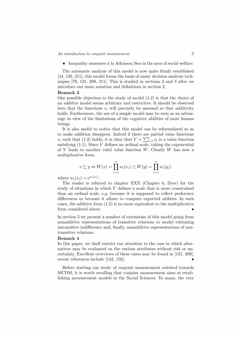
Choose any x02 ∈ X2. The, arbitrarily chosen, element (x0
1, x02) ∈ X
will be our “reference point”. The basic idea is to use this reference pointand the “unit” on the first attribute given by the reference preferenceinterval [x0
1, x11] to build a standard sequence on the preference intervals
on the second attribute. Hence, we are looking for an element x12 ∈ X2
that would be such that:
(x01, x
12) ∼ (x1
1, x02). (1.3)
Clearly this will require the structure of X2 to be adequately “rich” soas to find the level x1
2 ∈ X2 such that the reference preference interval onthe first attribute [x0
1, x11] is exactly matched by a preference interval of
the same “length” on the second attribute [x02, x
12]. Technically, this calls
for a solvability assumption or, more restrictively, for the suppositionthat X2 has a (topological) structure that is close to that of an intervalof R and that % is “somehow” continuous.
22
If such a level x12 can be found, model (1.2) implies:
v1(x01) + v2(x
12) = v1(x
11) + v2(x
02) so that
v2(x12) − v2(x
02) = v1(x
11) − v1(x
01).
(1.4)
Let us fix the origin of measurement letting:
v1(x01) = v2(x
02) = 0,
and our unit of measurement letting:
v1(x11) = 1 so that v1(x
11) − v1(x
01) = 1.
Using (1.4), we therefore obtain v2(x12) = 1. We have therefore found
an interval between levels on the second attribute ([x02, x
12]) that exactly
matches our reference interval on the first attribute ([x01, x
11]). We may
proceed to build our standard sequence on the second attribute (seeFigure 1.4) asking for levels x2
2, x32, . . . such that:
(x01, x
22) ∼ (x1
1, x12),
(x01, x
32) ∼ (x1
1, x22),
. . .
(x01, x
k2) ∼ (x1
1, xk−12 ).
As above, using (1.2) leads to:
v2(x22) − v2(x
12) = v1(x
11) − v1(x
01),
v2(x32) − v2(x
22) = v1(x
11) − v1(x
01),
. . .
v2(xk2) − v2(x
k−12 ) = v1(x
11) − v1(x
01),
so that:v2(x
22) = 2, v2(x
32) = 3, . . . , v2(x
k2) = k.
This process of building a standard sequence of the second attributetherefore leads to defining v2 on a number of, carefully, selected elementsof X2.
Remember the standard sequence that we built for length in section1.2. An implicit hypothesis was that the length of any rod could beexceeded by the length of a composite object obtained by concatenating asufficient number of perfect copies of a standard rod. Such an hypothesisis called “Archimedean” since it mimics the property of the real numbers
An introduction to conjoint measurement 23
x01
x02
X1
X2
x11
x12
x22
x32
x42
••
• •
••
••
•
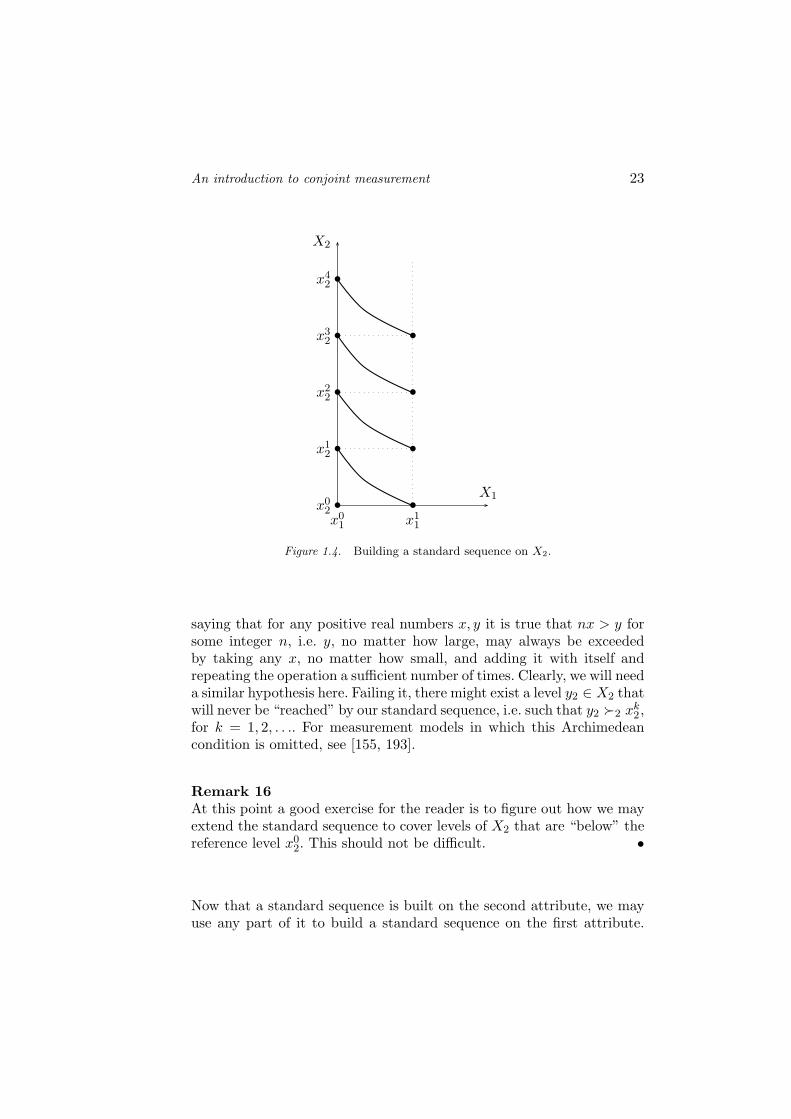
Figure 1.4. Building a standard sequence on X2.
saying that for any positive real numbers x, y it is true that nx > y forsome integer n, i.e. y, no matter how large, may always be exceededby taking any x, no matter how small, and adding it with itself andrepeating the operation a sufficient number of times. Clearly, we will needa similar hypothesis here. Failing it, there might exist a level y2 ∈ X2 thatwill never be “reached” by our standard sequence, i.e. such that y2 Â2 xk
2,for k = 1, 2, . . .. For measurement models in which this Archimedeancondition is omitted, see [155, 193].
Remark 16At this point a good exercise for the reader is to figure out how we mayextend the standard sequence to cover levels of X2 that are “below” thereference level x0
2. This should not be difficult. •
Now that a standard sequence is built on the second attribute, we mayuse any part of it to build a standard sequence on the first attribute.
24
x01
x02
X1
X2
x11 x2
1 x31 x3
1
x12 ••
•
•
•
•
• •
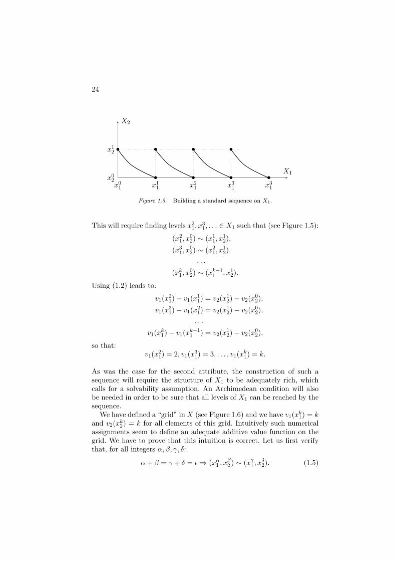
Figure 1.5. Building a standard sequence on X1.
This will require finding levels x21, x
31, . . . ∈ X1 such that (see Figure 1.5):
(x21, x
02) ∼ (x1
1, x12),
(x31, x
02) ∼ (x2
1, x12),
. . .
(xk1, x
02) ∼ (xk−1
1 , x12).
Using (1.2) leads to:
v1(x21) − v1(x
11) = v2(x
12) − v2(x
02),
v1(x31) − v1(x
21) = v2(x
12) − v2(x
02),
. . .
v1(xk1) − v1(x
k−11 ) = v2(x
12) − v2(x
02),
so that:v1(x
21) = 2, v1(x
31) = 3, . . . , v1(x
k1) = k.
As was the case for the second attribute, the construction of such asequence will require the structure of X1 to be adequately rich, whichcalls for a solvability assumption. An Archimedean condition will alsobe needed in order to be sure that all levels of X1 can be reached by thesequence.
We have defined a “grid” in X (see Figure 1.6) and we have v1(xk1) = k
and v2(xk2) = k for all elements of this grid. Intuitively such numerical
assignments seem to define an adequate additive value function on thegrid. We have to prove that this intuition is correct. Let us first verifythat, for all integers α, β, γ, δ:
α + β = γ + δ = ε ⇒ (xα1 , xβ
2 ) ∼ (xγ1 , xδ
2). (1.5)
An introduction to conjoint measurement 25
x01
x02
X1
X2
x11 x2
1 x31
x12
x22
x32
••
•
••
••
•
•
•
•
• •
?
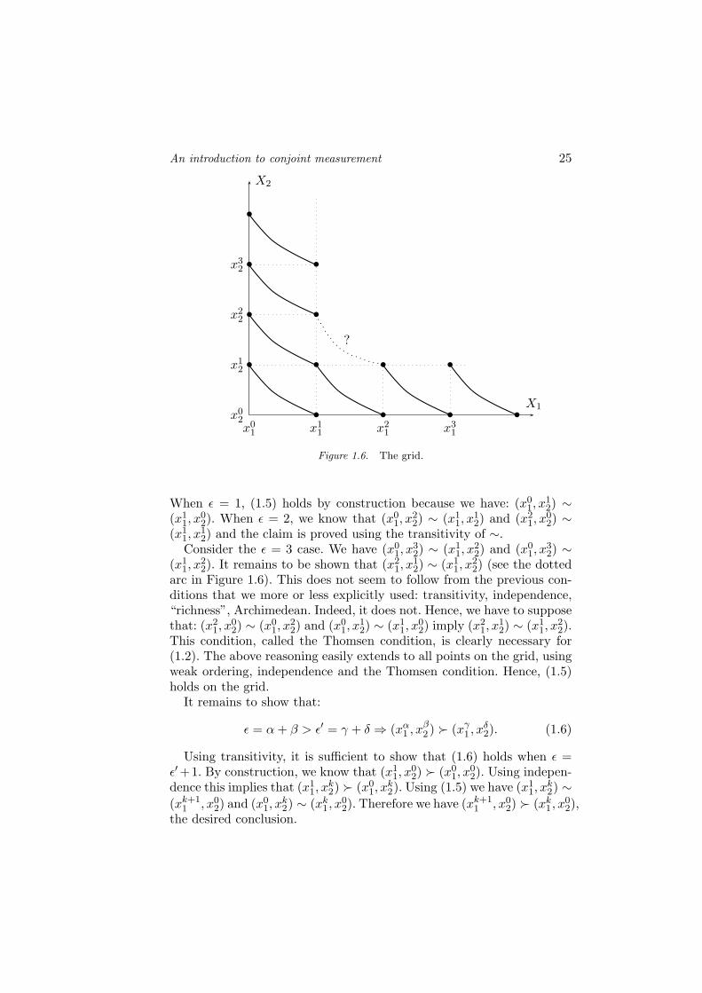
Figure 1.6. The grid.
When ε = 1, (1.5) holds by construction because we have: (x01, x
12) ∼
(x11, x
02). When ε = 2, we know that (x0
1, x22) ∼ (x1
1, x12) and (x2
1, x02) ∼
(x11, x
12) and the claim is proved using the transitivity of ∼.
Consider the ε = 3 case. We have (x01, x
32) ∼ (x1
1, x22) and (x0
1, x32) ∼
(x11, x
22). It remains to be shown that (x2
1, x12) ∼ (x1
1, x22) (see the dotted
arc in Figure 1.6). This does not seem to follow from the previous con-ditions that we more or less explicitly used: transitivity, independence,“richness”, Archimedean. Indeed, it does not. Hence, we have to supposethat: (x2
1, x02) ∼ (x0
1, x22) and (x0
1, x12) ∼ (x1
1, x02) imply (x2
1, x12) ∼ (x1
1, x22).
This condition, called the Thomsen condition, is clearly necessary for(1.2). The above reasoning easily extends to all points on the grid, usingweak ordering, independence and the Thomsen condition. Hence, (1.5)holds on the grid.
It remains to show that:
ε = α + β > ε′ = γ + δ ⇒ (xα1 , xβ
2 ) Â (xγ1 , xδ
2). (1.6)
Using transitivity, it is sufficient to show that (1.6) holds when ε =ε′ +1. By construction, we know that (x1
1, x02) Â (x0
1, x02). Using indepen-
dence this implies that (x11, x
k2) Â (x0
1, xk2). Using (1.5) we have (x1
1, xk2) ∼
(xk+11 , x0
2) and (x01, x
k2) ∼ (xk
1, x02). Therefore we have (xk+1
1 , x02) Â (xk
1, x02),
the desired conclusion.
26
x01
x02
X1
X2
x11 x2
1 x31 x4
1
x12
x22
x32
x42
•
•
•
•
•
•
•
••
••
•
•
•
•
• •
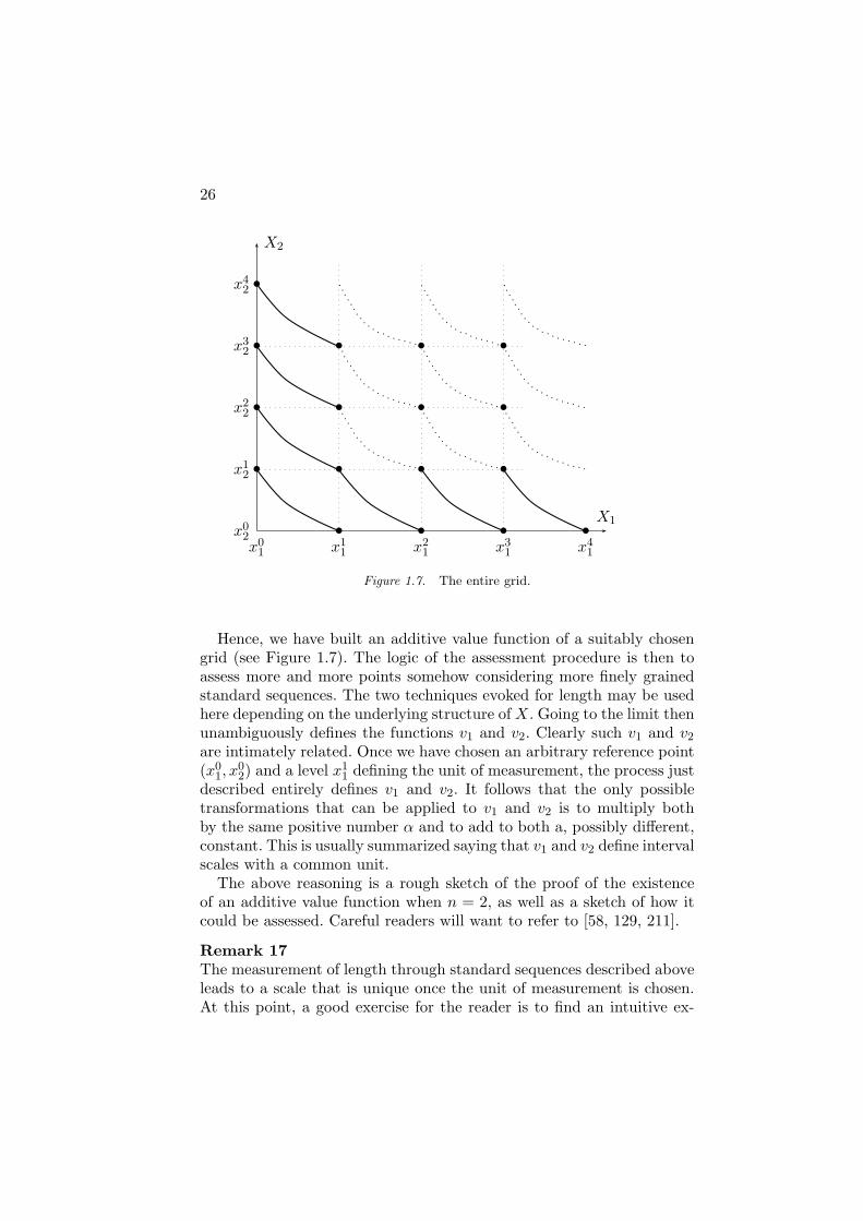
Figure 1.7. The entire grid.
Hence, we have built an additive value function of a suitably chosengrid (see Figure 1.7). The logic of the assessment procedure is then toassess more and more points somehow considering more finely grainedstandard sequences. The two techniques evoked for length may be usedhere depending on the underlying structure of X. Going to the limit thenunambiguously defines the functions v1 and v2. Clearly such v1 and v2
are intimately related. Once we have chosen an arbitrary reference point(x0
1, x02) and a level x1
1 defining the unit of measurement, the process justdescribed entirely defines v1 and v2. It follows that the only possibletransformations that can be applied to v1 and v2 is to multiply bothby the same positive number α and to add to both a, possibly different,constant. This is usually summarized saying that v1 and v2 define intervalscales with a common unit.
The above reasoning is a rough sketch of the proof of the existenceof an additive value function when n = 2, as well as a sketch of how itcould be assessed. Careful readers will want to refer to [58, 129, 211].
Remark 17The measurement of length through standard sequences described aboveleads to a scale that is unique once the unit of measurement is chosen.At this point, a good exercise for the reader is to find an intuitive ex-
An introduction to conjoint measurement 27
planation to the fact that, when measuring the “length” of preferenceintervals, the origin of measurement becomes arbitrary. The analogy withthe the measurement of duration on the one hand and dates, as given ina calendar, on the other hand should help. •
Remark 18As was already the case with the even swaps technique, it is worthemphasizing that this assessment technique makes no use of the vaguenotion of the “importance” of the various attributes. The “importance”is captured here in the lengths of the preference intervals on the variousattributes.
A common but critical mistake is to confuse the additive value func-tion model (1.2) with a weighted average and to try to assess weightsasking whether an attribute is “more important” than another. Thismakes no sense. •
3.1.2 The case of more than two attributes. The goodnews is that the process is exactly the same when there are more thantwo attributes. With one surprise: the Thomsen condition is no moreneeded to prove that the standard sequences defined on each attributelead to an adequate value function on the grid. A heuristic explanationof this strange result is that, when n = 2, there is no difference betweenindependence and weak independence. This is no more true when n ≥ 3and assuming independence is much stronger than just assuming weakindependence.
3.2. Statement of results
We use below the “algebraic approach” [127, 129, 141]. A more restrictiveapproach using a topological structure on X is given in [44, 58, 211]. Weformalize below the conditions informally introduced in the precedingsection. The reader not interested in the precise statement of the resultsor, better, having already written down his own statement, may skipthis section.Definition 19 (Thomsen condition)Let % be a binary relation on a set X = X1 × X2. It is said to satisfythe Thomsen condition if
(x1, x2) ∼ (y1, y2) and (y1, z2) ∼ (z1, x2) ⇒ (x1, z2) ∼ (z1, y2),
for all x1, y1, z1 ∈ X1 and all x2, y2, z2 ∈ X2.
Figure 1.8 shows how the Thomsen condition uses two “indifferencecurves” (i.e. curves linking points that are indifferent) to place a con-straint on a third one. This was needed above to prove that an additive
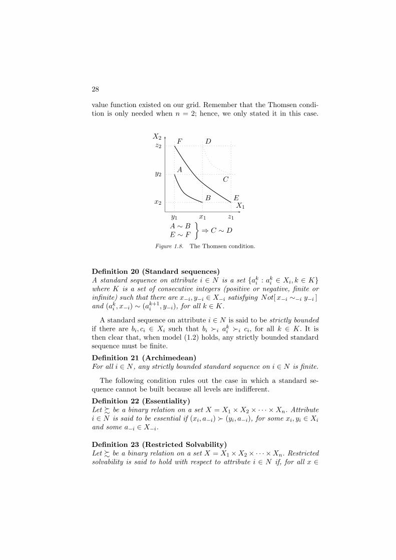
28
value function existed on our grid. Remember that the Thomsen condi-tion is only needed when n = 2; hence, we only stated it in this case.
X2
X1
y1 x1 z1
x2
y2
z2
A
B
C
D
E
F
A ∼ BE ∼ F
}
⇒ C ∼ D
Figure 1.8. The Thomsen condition.
Definition 20 (Standard sequences)A standard sequence on attribute i ∈ N is a set {ak
i : aki ∈ Xi, k ∈ K}
where K is a set of consecutive integers (positive or negative, finite orinfinite) such that there are x−i, y−i ∈ X−i satisfying Not[ x−i ∼−i y−i ]and (ak
i , x−i) ∼ (ak+1i , y−i), for all k ∈ K.
A standard sequence on attribute i ∈ N is said to be strictly boundedif there are bi, ci ∈ Xi such that bi Âi ak
i Âi ci, for all k ∈ K. It isthen clear that, when model (1.2) holds, any strictly bounded standardsequence must be finite.
Definition 21 (Archimedean)For all i ∈ N , any strictly bounded standard sequence on i ∈ N is finite.
The following condition rules out the case in which a standard se-quence cannot be built because all levels are indifferent.
Definition 22 (Essentiality)Let % be a binary relation on a set X = X1 × X2 × · · · × Xn. Attributei ∈ N is said to be essential if (xi, a−i) Â (yi, a−i), for some xi, yi ∈ Xi
and some a−i ∈ X−i.
Definition 23 (Restricted Solvability)Let % be a binary relation on a set X = X1 ×X2 × · · · ×Xn. Restrictedsolvability is said to hold with respect to attribute i ∈ N if, for all x ∈
An introduction to conjoint measurement 29
X, all z−i ∈ X−i and all ai, bi ∈ Xi, [(ai, z−i) % x % (bi, z−i)] ⇒[x ∼ (ci, z−i), for some ci ∈ Xi].
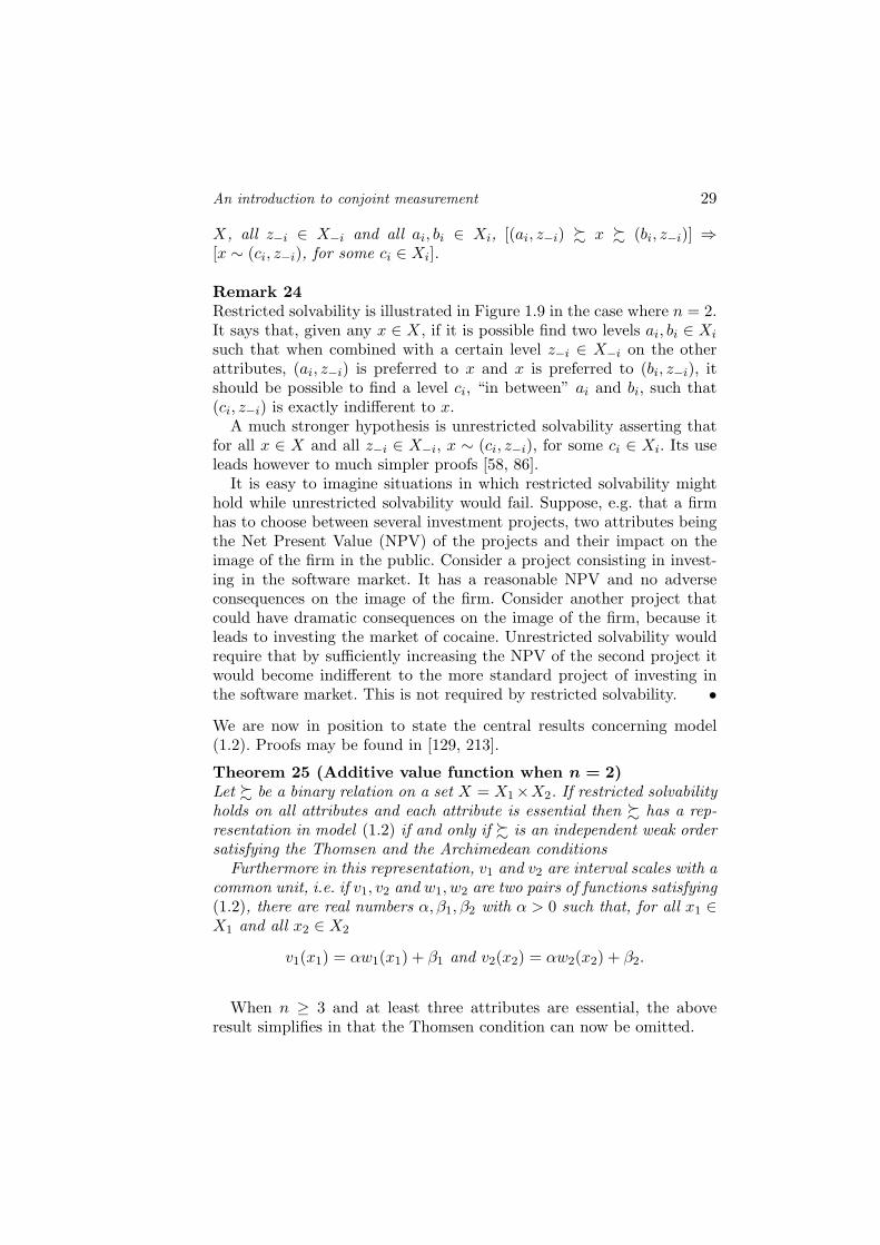
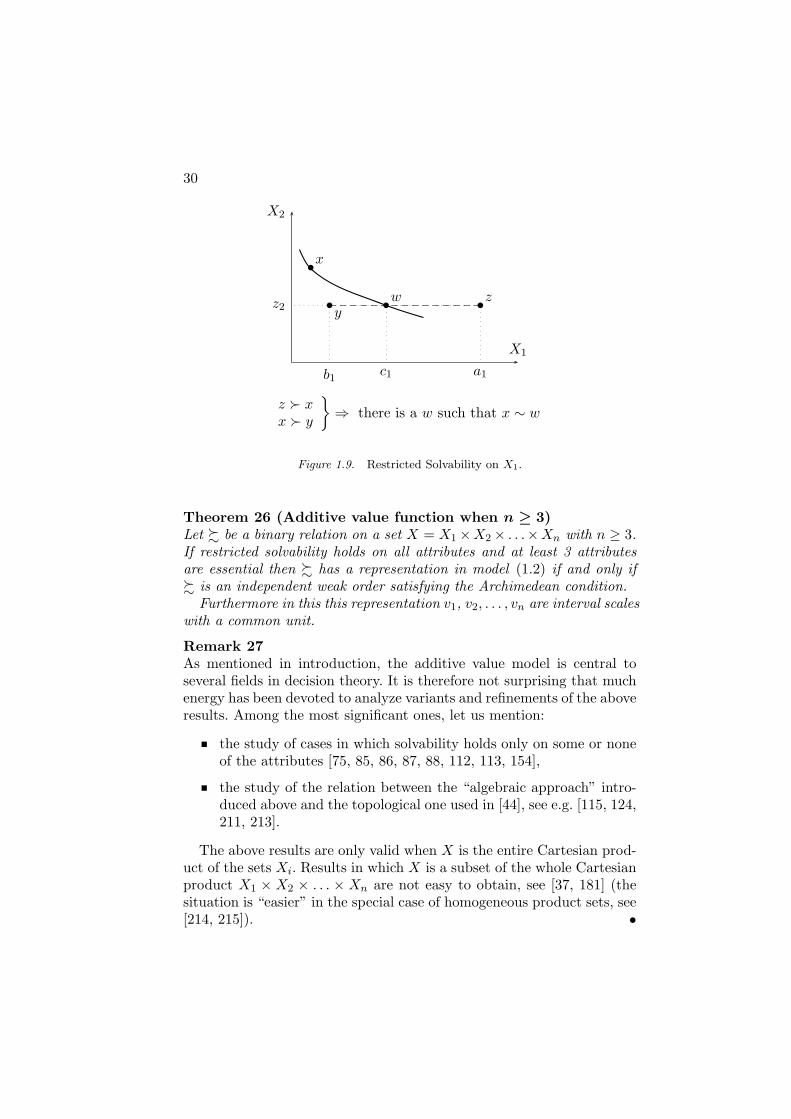
Remark 24Restricted solvability is illustrated in Figure 1.9 in the case where n = 2.It says that, given any x ∈ X, if it is possible find two levels ai, bi ∈ Xi
such that when combined with a certain level z−i ∈ X−i on the otherattributes, (ai, z−i) is preferred to x and x is preferred to (bi, z−i), itshould be possible to find a level ci, “in between” ai and bi, such that(ci, z−i) is exactly indifferent to x.
A much stronger hypothesis is unrestricted solvability asserting thatfor all x ∈ X and all z−i ∈ X−i, x ∼ (ci, z−i), for some ci ∈ Xi. Its useleads however to much simpler proofs [58, 86].
It is easy to imagine situations in which restricted solvability mighthold while unrestricted solvability would fail. Suppose, e.g. that a firmhas to choose between several investment projects, two attributes beingthe Net Present Value (NPV) of the projects and their impact on theimage of the firm in the public. Consider a project consisting in invest-ing in the software market. It has a reasonable NPV and no adverseconsequences on the image of the firm. Consider another project thatcould have dramatic consequences on the image of the firm, because itleads to investing the market of cocaine. Unrestricted solvability wouldrequire that by sufficiently increasing the NPV of the second project itwould become indifferent to the more standard project of investing inthe software market. This is not required by restricted solvability. •
We are now in position to state the central results concerning model(1.2). Proofs may be found in [129, 213].
Theorem 25 (Additive value function when n = 2)Let % be a binary relation on a set X = X1×X2. If restricted solvabilityholds on all attributes and each attribute is essential then % has a rep-resentation in model (1.2) if and only if % is an independent weak ordersatisfying the Thomsen and the Archimedean conditions
Furthermore in this representation, v1 and v2 are interval scales with acommon unit, i.e. if v1, v2 and w1, w2 are two pairs of functions satisfying(1.2), there are real numbers α, β1, β2 with α > 0 such that, for all x1 ∈X1 and all x2 ∈ X2
v1(x1) = αw1(x1) + β1 and v2(x2) = αw2(x2) + β2.
When n ≥ 3 and at least three attributes are essential, the aboveresult simplifies in that the Thomsen condition can now be omitted.
30
X1
X2
x•
z2
b1a1c1
w•y
•z
•
z  xx  y
}
⇒ there is a w such that x ∼ w
Figure 1.9. Restricted Solvability on X1.
Theorem 26 (Additive value function when n ≥ 3)Let % be a binary relation on a set X = X1 ×X2 × . . .×Xn with n ≥ 3.If restricted solvability holds on all attributes and at least 3 attributesare essential then % has a representation in model (1.2) if and only if% is an independent weak order satisfying the Archimedean condition.
Furthermore in this this representation v1, v2, . . . , vn are interval scaleswith a common unit.
Remark 27As mentioned in introduction, the additive value model is central toseveral fields in decision theory. It is therefore not surprising that muchenergy has been devoted to analyze variants and refinements of the aboveresults. Among the most significant ones, let us mention:
the study of cases in which solvability holds only on some or noneof the attributes [75, 85, 86, 87, 88, 112, 113, 154],
the study of the relation between the “algebraic approach” intro-duced above and the topological one used in [44], see e.g. [115, 124,211, 213].
The above results are only valid when X is the entire Cartesian prod-uct of the sets Xi. Results in which X is a subset of the whole Cartesianproduct X1 × X2 × . . . × Xn are not easy to obtain, see [37, 181] (thesituation is “easier” in the special case of homogeneous product sets, see[214, 215]). •
An introduction to conjoint measurement 31
3.3. Implementation: Standard sequences andbeyond
We have already shown above how additive value functions can be as-sessed using the standard sequence technique. It is worth recalling heresome of the characteristics of this assessment procedure:
It requires the set Xi to be rich so that it is possible to find apreference interval on Xi that will exactly match a preference in-terval on another attribute. This excludes using such an assessmentprocedure when some of the sets Xi are discrete.
It relies on indifference judgements which, a priori, are less firmlyestablished than preference judgements.
It relies on judgements concerning fictitious alternatives which,a priori, are harder to conceive than judgements concerning realalternatives.
The various assessments are thoroughly intertwined and, e.g., animprecision on the assessment of x1
2, i.e. the endpoint of the firstinterval in the standard sequence on X2 (see Figure 1.4) will prop-agate to many assessed values,
The assessment of tradeoffs may be plagued with cognitive biases,see [46, 197].
The assessment procedure based on standard sequences is thereforerather demanding; this should be no surprise given the proximity be-tween this form of measurement and extensive measurement illustratedabove on the case of length. Hence, the assessment procedure based onstandard sequences seems to be seldom used in the practice of deci-sion analysis [121, 209]. The literature on the experimental assessmentof additive value functions, see e.g. [197, 208, 216], suggests that thisassessment is a difficult task that may be affected by several cognitivebiases.
Many other simplified assessment procedures have been proposed thatare less firmly grounded in theory. In many of them, the assessment ofthe partial value functions vi relies on direct comparison of preferencedifferences without recourse to an interval on another attribute used asa “meter stick”. We refer to [50] for a theoretical analysis of these tech-niques. They are also studied in detail in Chapter XXX of this volume(Chapter 6, Dyer).
These procedures include:
direct rating techniques in which values of vi are directly assessedwith reference to two arbitrarily chosen points [52, 53],
32
procedures based on bisection, the decision-maker being asked toassess a point that is “half way” in terms of preference two refer-ence points [209],
procedures trying to build standard sequences on each attribute interms of “preference differences” [129, ch. 4].
An excellent overview of these techniques may be found in [209].
4. The additive value model in the “finite” case
4.1. Outline of theory
In this section, we suppose that % is a binary relation on a finite setX ⊆ X1 × X2 × · · · × Xn (contrary to the preceding section, dealingwith subsets of product sets will raise no difficulty here). The finitenesshypothesis clearly invalidates the standard sequence mechanism used tillnow. On each attribute there will only be finitely many “preference inter-vals” and exact matches between preference intervals will only happenexceptionally, see [212].
Clearly, independence remains a necessary condition for model (1.2)as before. Given the absence of structure of the set X, it is unlikely thatthis condition is sufficient to ensure (1.2). The following example showsthat this intuition is indeed correct.Example 28Let X = X1 × X2 with X1 = {a, b, c} and X2 = {d, e, f}. Consider theweak order on X such that, abusing notation in an obvious way,
ad  bd  ae  af  be  cd  ce  bf  cf.
It is easy to check that % is independent. Indeed, we may for instancecheck that:
ad  bd and ae  be and af  bf,
ad  ae and bd  be and cd  ce.
This relation cannot however be represented in model (1.2) since:
af  be ⇒ v1(a) + v2(f) > v1(b) + v2(e),
be  cd ⇒ v1(b) + v2(e) > v1(c) + v2(d),
ce  bf ⇒ v1(c) + v2(e) > v1(b) + v2(f),
bd  ae ⇒ v1(b) + v2(d) > v1(a) + v2(e).
Summing the first two inequalities leads to:
v1(a) + v2(f) > v1(c) + v2(d).

An introduction to conjoint measurement 33
Summing the last two inequalities leads to:
v1(c) + v2(d) > v1(a) + v2(f),
a contradiction.Note that, since no indifference is involved, the Thomsen condition is
trivially satisfied. Although it is clearly necessary for model (1.2), addingit to independence will therefore not solve the problem. 3
The conditions allowing to build an additive value model in the finitecase were investigated in [1, 2, 179]. Although the resulting conditionsturn out to be complex, the underlying idea is quite simple. It amountsto finding conditions under which a system of linear inequalities has asolution.
Suppose that x  y. If model (1.2) holds, this implies that:
n∑
i=1
vi(xi) >n
∑
i=1
vi(yi). (1.7)
Similarly if x ∼ y, we obtain:
n∑
i=1
vi(xi) =
n∑
i=1
vi(yi). (1.8)
The problem is then to find conditions on % such that the system offinitely many equalities and inequalities (1.7-1.8) has a solution. This isa classical problem in Linear Algebra [83].
Definition 29 (Relation Em)
Let m be an integer ≥ 2. Let x1, x2, . . . , xm, y1, y2, . . . , ym ∈ X. We saythat
(x1, x2, . . . , xm)Em(y1, y2, . . . , ym)
if, for all i ∈ N , (x1i , x
2i , . . . , x
mi ) is a permutation of (y1
i , y2i , . . . , y
mi ).
Suppose that (x1, x2, . . . , xm)Em(y1, y2, . . . , ym) then model (1.2) im-plies that
m∑
j=1
n∑
i=1
vi(xji ) =
m∑
j=1
n∑
i=1
vi(yji ).
Therefore if xj % yj for j = 1, 2, . . . , m − 1, it cannot be true thatxm  ym. This condition must hold for all m = 2, 3, . . ..
34
Definition 30 (Condition Cm)
Let m be an integer ≥ 2. We say that condition Cm holds if
[xj % yj for j = 1, 2, . . . , m − 1] ⇒ Not[ xm  ym ]
for all x1, x2, . . . , xm, y1, y2, . . . , ym ∈ X such that
(x1, x2, . . . , xm)Em(y1, y2, . . . , ym).
Remark 31It is not difficult to check that:
Cm+1 ⇒ Cm,
C2 ⇒ % is independent,
C3 ⇒ % is transitive. •
We already observed that Cm was implied by the existence of anadditive representation. The main result for the finite case states thatrequiring that % is complete and that Cm holds for m = 2, 3, . . . is alsosufficient. Proofs can be found in [58, 129].
Theorem 32Let % be a binary relation on a finite set X ⊆ X1×X2×· · ·×Xn. Thereare real-valued functions vi on Xi such that (1.2) holds if and only if %is complete and satisfies Cm for m = 2, 3, . . ..
Remark 33Contrary to the “rich” case considered in the preceding section, we havehere necessary and sufficient conditions for the additive value model(1.2). However, it is important to notice that the above result uses adenumerable scheme of conditions. It is shown in [180] that this denu-merable scheme cannot be truncated: for all m ≥ 2, there is a relation %on a finite set X such that Cm holds but violating Cm+1. This is studiedin more detail in [139, 201, 218]. Therefore, no finite scheme of axiomsis sufficient to characterize model (1.2) for all finite sets X.
Given a finite set X of given cardinality, it is well-known that thedenumerable scheme of condition can be truncated. The precise relationbetween the cardinality of X and the number of conditions needed raisesdifficult combinatorial questions that are studied in [77, 78]. •
Remark 34It is clear that, if a relation % has a representation in model (1.2) withfunctions vi, it also has a representation using functions v′i = αvi + βi
with α > 0. Contrary to the rich case, the uniqueness of the functionsvi is more complex as shown by the following example.
An introduction to conjoint measurement 35
Example 35Let X = X1 × X2 with X1 = {a, b, c} and X2 = {d, e}. Consider theweak order on X such that, abusing notation in an obvious way,
ad  bd  ae  cd  be  ce.
This relation has a representation in model (1.2) with
v1(a) = 3, v1(b) = 1, v1(c) = 0, v2(d) = 3, v2(e) = 0.5.
An equally valid representation would be given taking v1(b) = 2. Clearlythis new representation cannot be deduced from the original one apply-ing a positive affine transformation. 3
Remark 36Theorem 32 has been extended to the case of an arbitrary set X in[113, 112], see also [75, 81]. The resulting conditions are however quitecomplex. This explains why we spent time on this “rich” case in thepreceding section. •
Remark 37The use of a denumerable scheme of conditions in theorem 32 does notfacilitate the interpretation and the test of conditions. However it shouldbe noticed that, on a given set X, the test of the Cm conditions amountsto finding if a system of finitely many linear inequalities has a solution.It is well-known that Linear Programming techniques are quite efficientfor such a task. •
4.2. Implementation: LP-based assessment
We show how to use LP techniques in order to assess an additive valuemodel (1.2), without supposing that the sets Xi are rich. For practicalpurposes, it is not restrictive to assume that we are only interested inassessing a model for a limited range on each Xi. We therefore assumethat the sets Xi are bounded so that, using independence, there is aworst value xi∗ and a most preferable value x∗
i . Using the uniquenessproperties of model (1.2), we may always suppose, after an appropriatenormalization, that:
v1(x1∗) = v2(x2∗) = . . . = vn(xn∗) = 0 and (1.9)n
∑
i=1
vi(x∗i ) = 1. (1.10)
Two main cases arise (see Figures 1.10 and 1.11):
36
vi(xi)
xixi∗ x1
i x2i x∗
i
vi(xi∗)
vi(x1i )
vi(x2i )
vi(x∗i )
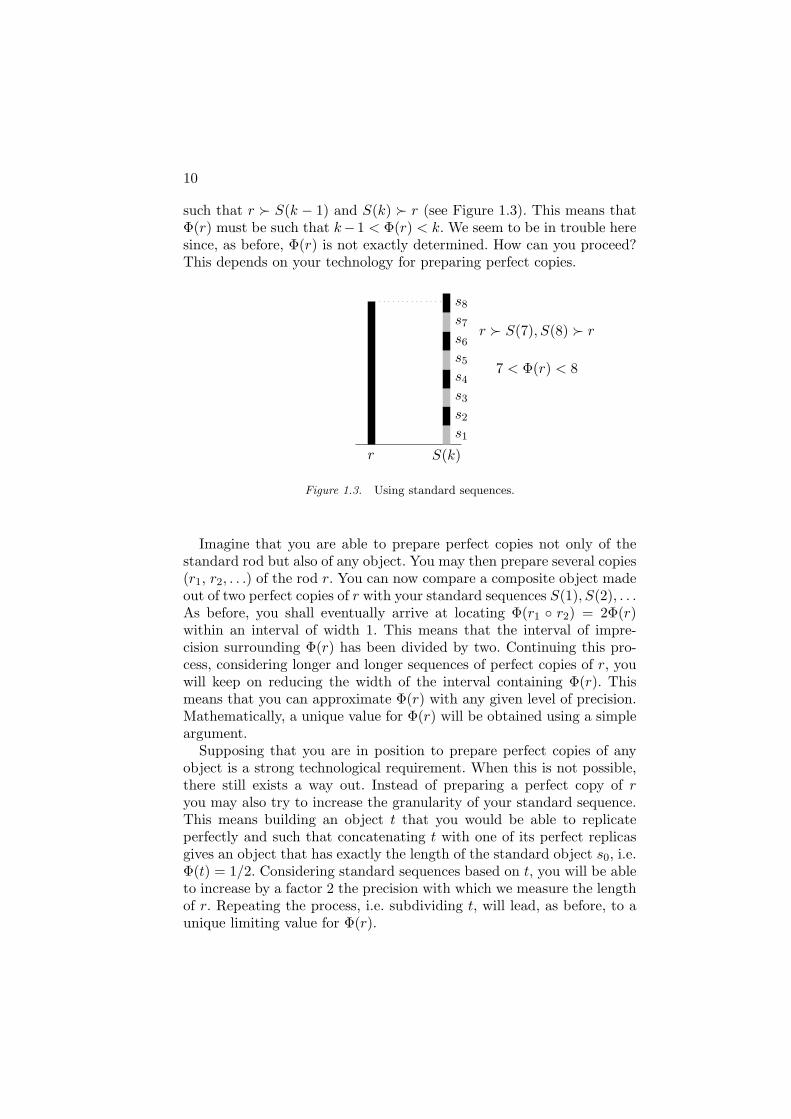
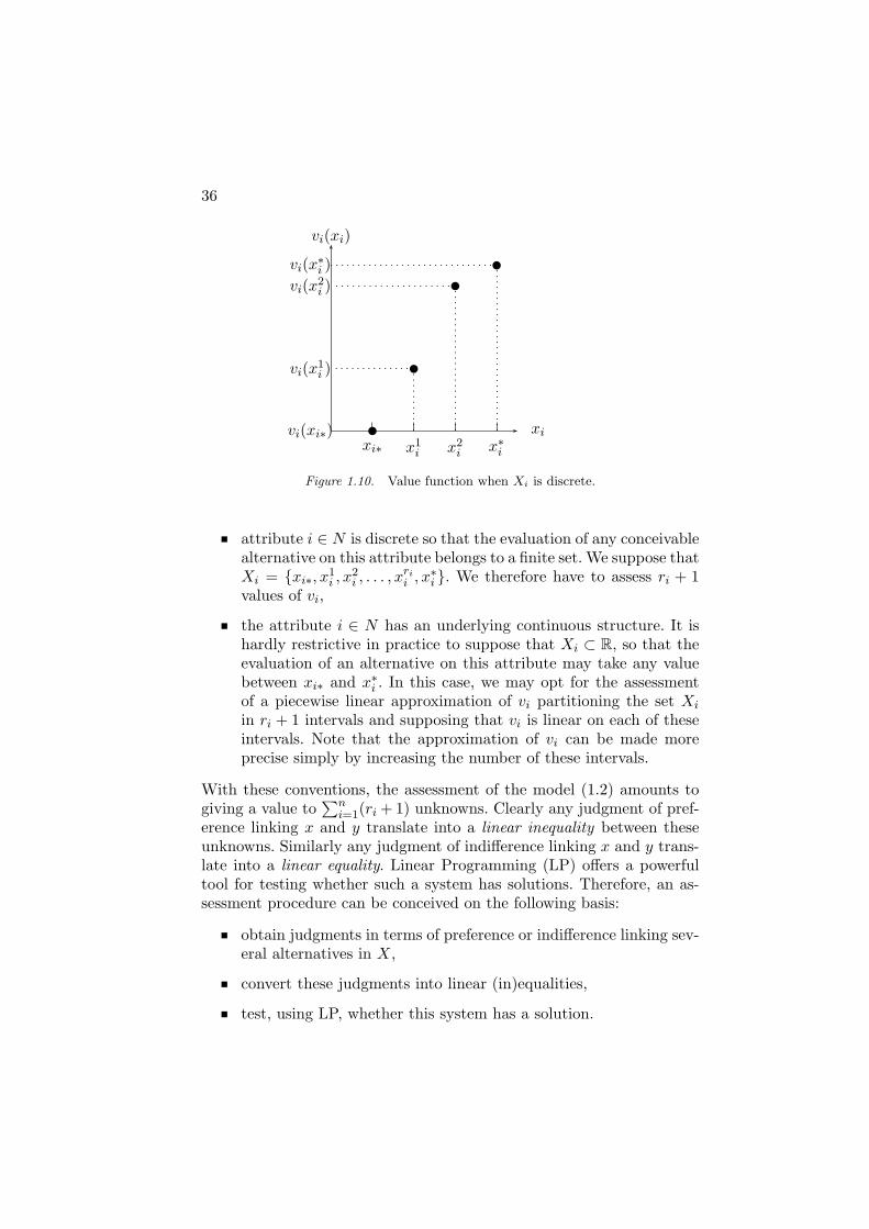
Figure 1.10. Value function when Xi is discrete.
attribute i ∈ N is discrete so that the evaluation of any conceivablealternative on this attribute belongs to a finite set. We suppose thatXi = {xi∗, x
1i , x
2i , . . . , x
ri
i , x∗i }. We therefore have to assess ri + 1
values of vi,
the attribute i ∈ N has an underlying continuous structure. It ishardly restrictive in practice to suppose that Xi ⊂ R, so that theevaluation of an alternative on this attribute may take any valuebetween xi∗ and x∗
i . In this case, we may opt for the assessmentof a piecewise linear approximation of vi partitioning the set Xi
in ri + 1 intervals and supposing that vi is linear on each of theseintervals. Note that the approximation of vi can be made moreprecise simply by increasing the number of these intervals.
With these conventions, the assessment of the model (1.2) amounts togiving a value to
∑ni=1(ri + 1) unknowns. Clearly any judgment of pref-
erence linking x and y translate into a linear inequality between theseunknowns. Similarly any judgment of indifference linking x and y trans-late into a linear equality. Linear Programming (LP) offers a powerfultool for testing whether such a system has solutions. Therefore, an as-sessment procedure can be conceived on the following basis:
obtain judgments in terms of preference or indifference linking sev-eral alternatives in X,
convert these judgments into linear (in)equalities,
test, using LP, whether this system has a solution.
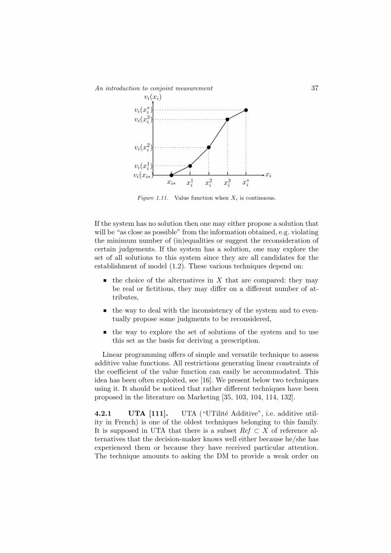
An introduction to conjoint measurement 37vi(xi)
xixi∗ x1
i x2i x3
i x∗i
vi(xi∗)
vi(x1i )
vi(x2i )
vi(x3i )
vi(x∗i )
Figure 1.11. Value function when Xi is continuous.
If the system has no solution then one may either propose a solution thatwill be “as close as possible” from the information obtained, e.g. violatingthe minimum number of (in)equalities or suggest the reconsideration ofcertain judgements. If the system has a solution, one may explore theset of all solutions to this system since they are all candidates for theestablishment of model (1.2). These various techniques depend on:
the choice of the alternatives in X that are compared: they maybe real or fictitious, they may differ on a different number of at-tributes,
the way to deal with the inconsistency of the system and to even-tually propose some judgments to be reconsidered,
the way to explore the set of solutions of the system and to usethis set as the basis for deriving a prescription.
Linear programming offers of simple and versatile technique to assessadditive value functions. All restrictions generating linear constraints ofthe coefficient of the value function can easily be accommodated. Thisidea has been often exploited, see [16]. We present below two techniquesusing it. It should be noticed that rather different techniques have beenproposed in the literature on Marketing [35, 103, 104, 114, 132].
4.2.1 UTA [111]. UTA (“UTilite Additive”, i.e. additive util-ity in French) is one of the oldest techniques belonging to this family.It is supposed in UTA that there is a subset Ref ⊂ X of reference al-ternatives that the decision-maker knows well either because he/she hasexperienced them or because they have received particular attention.The technique amounts to asking the DM to provide a weak order on
38
Ref . Each preference or indifference relation contained in this weak orderis then translated into a linear constraint:
x ∼ y gives an equality v(x) − v(y) = 0 and
x  y gives an inequality v(x) − v(y) > 0,
where v(x) and v(y) can be expressed as a linear combination of theunknowns as remarked earlier. Strict inequalities are then translated intolarge inequalities as is usual in Linear Programming, i.e. v(x)−v(y) > 0becomes v(x) − v(y) ≥ ε where ε > 0 is a very small positive numberthat should be chosen according to the precision of the arithmetics usedby the LP package.
The test of the existence of a solution to the system of linear con-straints is done via standard Goal Programming techniques [36] addingappropriate deviation variables. In UTA, each equation v(x) − v(y) = 0is translated into an equation v(x)−v(y)+σ+
x −σ−x +σ+
y −σ−y = 0, where
σ+x , σ−
x , σ+y and σ−
y are nonnegative deviation variables. Similarly each
inequality v(x)−v(y) ≥ ε is written as v(x)−v(y)+σ+x −σ−
x +σ+y −σ−
y ≥ ε.It is clear that there will exist a solution to the original system of linearconstraints if there is a solution of the LP in which all deviation variablesare zero. This can easily be tested using the objective function
Minimize Z =∑
x∈Ref
σ+x + σ−
x (1.11)
Two cases arise. If the optimal value of Z is 0, there is an additivevalue function that represents the preference information. It should beobserved that, except in exceptional cases (e.g. if the preference infor-mation collected is identical to the preference information collected withthe standard sequence technique), there are infinitely many such additivevalue functions (that are not related via a simple change of origin and ofunit, since we already fixed them through normalization (1.9-1.10)). Theone given as the “optimal” one by the LP does not have a special statussince it is highly dependent upon the arbitrary choice of the objectivefunction; instead of minimizing the sum of the deviation variables, wecould have as well, and still preserving linearity, minimized the largest ofthese variables. The whole polyhedron of feasible solutions of the original(in)equalities corresponds to adequate additive value functions: we havea whole set V of additive value functions representing the informationcollected on the set of reference alternatives Ref .
The size of V is clearly dependent upon the choice of the alternativesin Ref . Using standard techniques in LP, several functions in V maybe obtained, e.g. the ones maximizing or minimizing, within V, vi(x
∗i )
An introduction to conjoint measurement 39
for each attribute [111]. It is often interesting to present them to thedecision-maker in the pictorial form of Figures 1.10 and 1.11.
If the optimal value of Z is strictly greater than 0, there is no additivevalue function representing the preference information available. The so-lution given as optimal (note that it is not guaranteed that this solutionleads to the minimum possible number of violations w.r.t. the informa-tion provided—this would require solving an integer linear programme)is, in general, highly dependent upon the choice of the objective function.
This absence of solution to the system might be due to several factors:
the piecewise linear approximation of the vi for the “continuous”attributes may be too rough. It is easy to test whether an increasein the number of linear pieces on some of these attributes may leadto a nonempty set of additive value functions.
the information provided by the decision-maker may be of poorquality. It might then be interesting to present to the decision-maker one additive value function (e.g. one may present an averagefunction after some post-optimality analysis) in the pictorial formof Figures 1.10 and 1.11 and to let him react to this informationeither by modifying his/her initial judgments or even by lettinghim/her react directly on the shape of the value functions. This isthe solution implemented in the well-known PREFCALC system[109].
the preference provided by the decision-maker might be inconsis-tent with the conditions implied by an additive value function. Thesystem should then help locate these inconsistencies and allow theDM to think about them. Alternatively, since many alternativeattribute descriptions are possible, it may be worth investigatingwhether a different definition of the various attributes may lead toa preference model consistent with model (1.2). Several examplesof such analysis may be found in [119, 121, 209]
When the above techniques fail, the optimal solution of the LP, even ifnot compatible with the information provided, may still be consideredas an adequate model. Again, since the objective function introducedabove is somewhat arbitrary and it is recommended in [111] to performa post-optimality analysis, e.g. considering additive value functions thatare “close” to the optimal solution through the introduction of a linearconstraint:
Z ≤ Z∗ + δ,
where Z∗ is the optimal value of the objective function of the original LPand δ is a “small” positive number. As above, the result of the analysis is
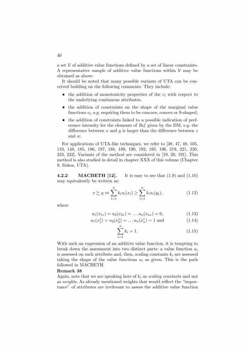
40
a set V of additive value functions defined by a set of linear constraints.A representative sample of additive value functions within V may beobtained as above.
It should be noted that many possible variants of UTA can be con-ceived building on the following comments. They include:
the addition of monotonicity properties of the vi with respect tothe underlying continuous attributes,
the addition of constraints on the shape of the marginal valuefunctions vi, e.g. requiring them to be concave, convex or S-shaped,
the addition of constraints linked to a possible indication of pref-erence intensity for the elements of Ref given by the DM, e.g. thedifference between x and y is larger than the difference between zand w.
For applications of UTA-like techniques, we refer to [38, 47, 48, 105,110, 148, 185, 186, 187, 188, 189, 190, 192, 195, 196, 219, 221, 220,223, 222]. Variants of the method are considered in [19, 20, 191]. Thismethod is also studied in detail in chapter XXX of this volume (Chapter9, Siskos, UTA).
4.2.2 MACBETH [12]. It is easy to see that (1.9) and (1.10)may equivalently be written as:
x % y ⇔n
∑
i=1
kiui(xi) ≥n
∑
i=1
kiui(yi), (1.12)
where
u1(x1∗) = u2(x2∗) = . . . un(xn∗) = 0, (1.13)
u1(x∗1) = u2(x
∗2) = . . . un(x∗
n) = 1 and (1.14)n
∑
i=1
ki = 1. (1.15)
With such an expression of an additive value function, it is tempting tobreak down the assessment into two distinct parts: a value function ui
is assessed on each attribute and, then, scaling constants ki are assessedtaking the shape of the value functions ui as given. This is the pathfollowed in MACBETH.
Remark 38Again, note that we are speaking here of ki as scaling constants and notas weights. As already mentioned weights that would reflect the “impor-tance” of attributes are irrelevant to assess the additive value function
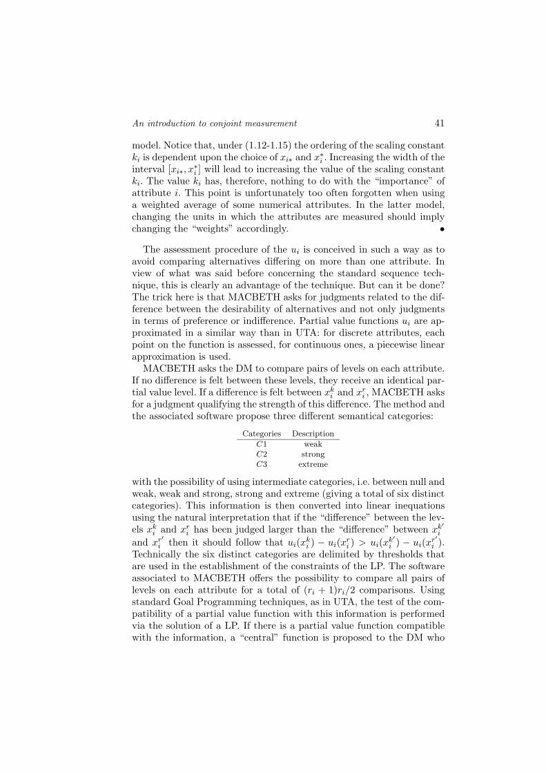
An introduction to conjoint measurement 41
model. Notice that, under (1.12-1.15) the ordering of the scaling constantki is dependent upon the choice of xi∗ and x∗
i . Increasing the width of theinterval [xi∗, x
∗i ] will lead to increasing the value of the scaling constant
ki. The value ki has, therefore, nothing to do with the “importance” ofattribute i. This point is unfortunately too often forgotten when usinga weighted average of some numerical attributes. In the latter model,changing the units in which the attributes are measured should implychanging the “weights” accordingly. •
The assessment procedure of the ui is conceived in such a way as toavoid comparing alternatives differing on more than one attribute. Inview of what was said before concerning the standard sequence tech-nique, this is clearly an advantage of the technique. But can it be done?The trick here is that MACBETH asks for judgments related to the dif-ference between the desirability of alternatives and not only judgmentsin terms of preference or indifference. Partial value functions ui are ap-proximated in a similar way than in UTA: for discrete attributes, eachpoint on the function is assessed, for continuous ones, a piecewise linearapproximation is used.
MACBETH asks the DM to compare pairs of levels on each attribute.If no difference is felt between these levels, they receive an identical par-tial value level. If a difference is felt between xk
i and xri , MACBETH asks
for a judgment qualifying the strength of this difference. The method andthe associated software propose three different semantical categories:
Categories Description
C1 weakC2 strongC3 extreme
with the possibility of using intermediate categories, i.e. between null andweak, weak and strong, strong and extreme (giving a total of six distinctcategories). This information is then converted into linear inequationsusing the natural interpretation that if the “difference” between the lev-els xk
i and xri has been judged larger than the “difference” between xk′
i
and xr′i then it should follow that ui(x
ki ) − ui(x
ri ) > ui(x
k′
i ) − ui(xr′i ).
Technically the six distinct categories are delimited by thresholds thatare used in the establishment of the constraints of the LP. The softwareassociated to MACBETH offers the possibility to compare all pairs oflevels on each attribute for a total of (ri + 1)ri/2 comparisons. Usingstandard Goal Programming techniques, as in UTA, the test of the com-patibility of a partial value function with this information is performedvia the solution of a LP. If there is a partial value function compatiblewith the information, a “central” function is proposed to the DM who
42
has the possibility to modify it. If not, the results of the LP are exploitedin such a way to propose modifications of the information that wouldmake it consistent.
The assessment of the scaling constant ki is done using similar princi-ples. The DM is asked to compare the following (n + 2) alternatives bypairs:
(x1∗, x2∗, . . . , xn∗),
(x∗1, x2∗, . . . , xn∗),
(x1∗, x∗2, . . . , xn∗),
. . .
(x1∗, x2∗, . . . , x∗n) and
(x∗1, x
∗2, . . . , x
∗n),
placing each pair in a category of difference. This information imme-diately translates into a set of linear constraints on the ki. These con-straints are processed as before. It should be noticed that, once thepartial value functions ui are assessed, it is not necessary to use the lev-els xi∗ and x∗
i to assess the ki since they may well lead to alternativesthat are too unrealistic. The authors of MACBETH suggest to replacexi∗ by a “neutral” level which appears neither desirable nor undesirableand x∗
i by a “desirable” level that is judged satisfactory. Although thisclearly impacts the quality of the dialogue with the DM, this has noconsequence on the underlying technique used to process information.
We refer to [6, 7, 8, 9, 10, 11] for applications of the MACBETHtechnique. This method is also studied in detail in chapter XXX of thisvolume (Chapter 10, Bana, MACBETH).
5. Extensions
The additive value model (1.2) is the central model for the applicationof conjoint measurement techniques to decision analysis. In this section,we consider various extensions to this model.
5.1. Transitive Decomposable models
The transitive decomposable model has been introduced in [129] as anatural generalization of model (1.2). It amounts to replacing the ad-dition operation by a general function that is increasing in each of itsarguments.
Definition 39 (Transitive decomposable model)Let % be a binary relation on a set X =
∏ni=1 Xi. The transitive decom-
posable model holds if, for all i ∈ N , there is a real-valued function vi
An introduction to conjoint measurement 43
on Xi and a real-valued function g on∏n
i=1 vi(Xi) that is increasing inall its arguments such that:
x % y ⇔ g(v1(x1), . . . , vn(xn)) ≥ g(v1(y1), . . . , vn(yn)), (1.16)
for all x, y ∈ X.
An interesting point with this model is that it admits an intuitivelyappealing simple characterization. The basic axiom for characterizingthe above transitive decomposable model is weak independence, whichis clearly implied by (1.16). The following theorem is proved in [129, ch.7].
Theorem 40A preference relation % on a finite or countably infinite set X has arepresentation in the transitive decomposable model iff % is a weaklyindependent weak order.
Remark 41This result can be extended to sets of arbitrary cardinality adding a,necessary, condition implying that the weak order % has a numericalrepresentation, see [42, 45]. •
The weak point of such a model is that the function g is left unspecifiedso that the model will be difficult to assess. Furthermore, the uniquenessresults for vi and g are clearly much less powerful than what we obtainedwith model (1.2), see [129, ch. 7]. Therefore, practical applications ofthis model generally imply specifying the type of function g, possiblyby verifying further conditions on the preference relation that imposethat g belongs to some parameterized family of functions, e.g. somepolynomial function of the vi. This is studied in detail in [129, ch. 7] and[14, 82, 139, 138, 156, 166, 202]. Since such models have, to the best ofour knowledge, never been used in decision analysis, we do not analyzethem further.
The structure of the decomposable model however suggests that as-sessment techniques for this model could well come from Artificial Intelli-gence with its “rule induction” machinery. Indeed the function g in model(1.16) may also be seen as a set of “rules”. We refer to [97, 98, 100, 101]for a thorough study of the potentiality of such an approach.
Remark 42A simple extension of the decomposable model consists in simply askingfor a function g that would be nondecreasing in each of its arguments.The following result is proved in [30] (see also [100]) (it can easily beextended to cover the case of an arbitrary set X, adding a, necessary,condition implying that % has a numerical representation).
44
We say that % is weakly separable if, for all i ∈ N and all xi, yi ∈ Xi, itis never true that (xi, z−i) Â (yi, z−i) and (yi, w−i) Â (xi, w−i), for somez−i, w−i ∈ X−i. Clearly this is a weakening of weak independence sinceit tolerates to have at the same time (xi, z−i) Â (yi, z−i) and (xi, w−i) ∼(yi, w−i).
Theorem 43A preference relation % on a finite or countably infinite set X has arepresentation in the weak decomposable model:
x % y ⇔ g(u1(x1), . . . , un(xn)) ≥ g(u1(y1), . . . , un(yn))
with g nondecreasing in all its arguments iff % is a weakly separable weakorder.
A recent trend of research has tried to characterize special functionalforms for g in the weakly decomposable model, such as max, min orsome more complex forms. The main references include [26, 100, 102,182, 194]. •
Remark 44The use of “fuzzy integrals” as tools for aggregating criteria has recentlyattracted much attention [49, 90, 91, 93, 94, 95, 143, 145, 144, 146], theChoquet Integral and the Sugeno integral being among the most popu-lar. It should be strongly emphasized that the very definition of theseintegrals requires to have at hand a weak order on ∪n
i=1Xi, supposingw.l.o.g. that the sets Xi are disjoint. This is usually called a “commen-surability hypothesis”. Whereas this hypothesis is quite natural whendealing with an homogeneous Cartesian product, as in decision underuncertainty (see e.g. [211]), it is far less so in the area of multiple cri-teria decision making. A neat conjoint measurement analysis of suchmodels and their associated assessment procedures is an open researchquestion, see [92]. •
5.2. Intransitive indifference
Decomposable models form a large family of preferences though notlarge enough to encompass all cases that may be encountered when ask-ing subjects to express preferences. A major restriction is that not allpreferences may be assumed to be weak orders. The example of thesequence of cups of coffee, each differing from the previous one by animperceptible quantity of sugar added [133], is famous; it leads to the
An introduction to conjoint measurement 45
notions of semiorder and interval order [4, 57, 66, 133, 161], in whichindifference is not transitive, while strict preference is.
Ideally, taking intransitive indifference into account, we would wantto arrive at a generalization of (1.2) in which:
x ∼ y ⇔ |V (x) − V (y)| ≤ ε,
x  y ⇔ V (x) > V (y) + ε,
where ε ≥ 0 and V (x) =∑n
i=1 vi(xi).In the finite case, it is not difficult to extend the conditions presented
in section 4 to cover such a case. Indeed, we are still looking here forthe solution to a system of linear constraints. Although this seems tohave never been done, it would not be difficult to adapt the LP-basedassessment techniques to this case.
On the contrary, extending the standard sequence technique of sec-tion 3 is a formidable challenge. Indeed, remember that these techniquescrucially rest on indifference judgments which lead to the determinationof “perfect copies” of a given preference interval. As soon as indifferenceis not supposed to be transitive, “perfect copies” are not so perfect andmuch trouble is expected. We refer to [84, 128, 134, 161, 198] for a studyof these models.
Remark 45Even if the analysis of such models proves difficult, it should be notedthat the semi-ordered version of the additive value model may be inter-preted as having a “built-in” sensitivity analysis via the introduction ofthe threshold ε. Therefore, in practice, we may usefully view ε not as aparameter to be assessed but as a simple trick to avoid undue discrimi-nation, because of the imprecision inevitably involved in our assessmentprocedures, between close alternatives •
Remark 46Clearly the above model can be generalized to cope with a possiblynon-constant threshold. The literature on the subject remains minimalhowever, see [161]. •
5.3. Nontransitive preferences
Many authors [147, 203] have argued that the reasonableness of suppos-ing that strict preference is transitive is not so strong when it comes tocomparing objects evaluated on several attributes. As soon as it is sup-posed that subjects may use an “ordinal” strategy for comparing objects,examples inspired from the well-known Condorcet paradox [176, 183]show that intransitivities will be difficult to avoid. Indeed it is possi-ble to observe predictable intransitivities of strict preference in carefully
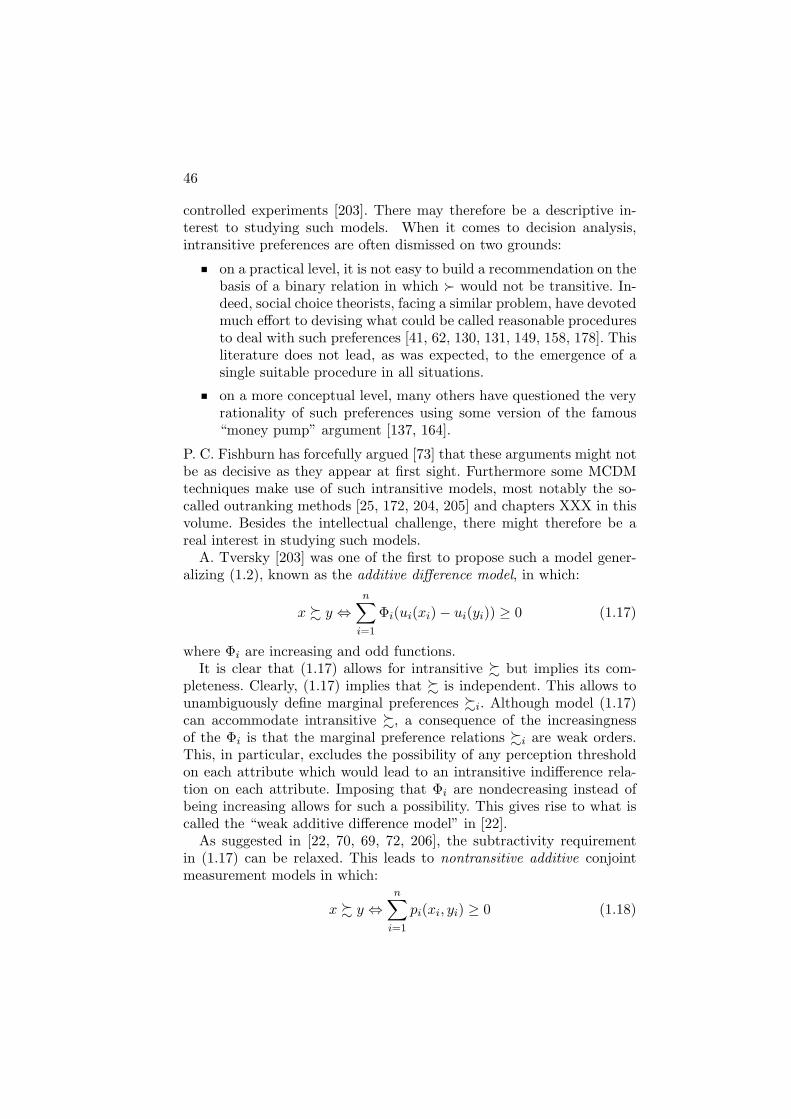
46
controlled experiments [203]. There may therefore be a descriptive in-terest to studying such models. When it comes to decision analysis,intransitive preferences are often dismissed on two grounds:
on a practical level, it is not easy to build a recommendation on thebasis of a binary relation in which  would not be transitive. In-deed, social choice theorists, facing a similar problem, have devotedmuch effort to devising what could be called reasonable proceduresto deal with such preferences [41, 62, 130, 131, 149, 158, 178]. Thisliterature does not lead, as was expected, to the emergence of asingle suitable procedure in all situations.
on a more conceptual level, many others have questioned the veryrationality of such preferences using some version of the famous“money pump” argument [137, 164].
P. C. Fishburn has forcefully argued [73] that these arguments might notbe as decisive as they appear at first sight. Furthermore some MCDMtechniques make use of such intransitive models, most notably the so-called outranking methods [25, 172, 204, 205] and chapters XXX in thisvolume. Besides the intellectual challenge, there might therefore be areal interest in studying such models.
A. Tversky [203] was one of the first to propose such a model gener-alizing (1.2), known as the additive difference model, in which:
x % y ⇔n
∑
i=1
Φi(ui(xi) − ui(yi)) ≥ 0 (1.17)
where Φi are increasing and odd functions.It is clear that (1.17) allows for intransitive % but implies its com-
pleteness. Clearly, (1.17) implies that % is independent. This allows tounambiguously define marginal preferences %i. Although model (1.17)can accommodate intransitive %, a consequence of the increasingnessof the Φi is that the marginal preference relations %i are weak orders.This, in particular, excludes the possibility of any perception thresholdon each attribute which would lead to an intransitive indifference rela-tion on each attribute. Imposing that Φi are nondecreasing instead ofbeing increasing allows for such a possibility. This gives rise to what iscalled the “weak additive difference model” in [22].
As suggested in [22, 70, 69, 72, 206], the subtractivity requirementin (1.17) can be relaxed. This leads to nontransitive additive conjointmeasurement models in which:
x % y ⇔n
∑
i=1
pi(xi, yi) ≥ 0 (1.18)
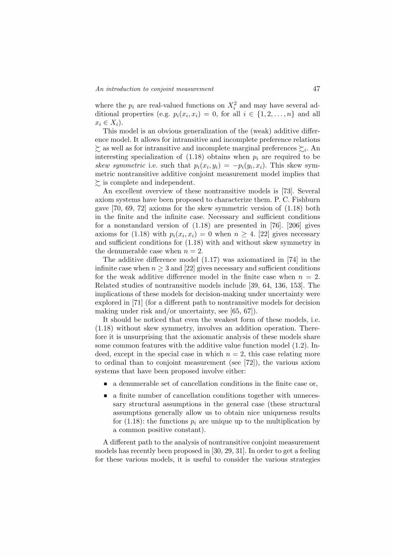
An introduction to conjoint measurement 47
where the pi are real-valued functions on X2i and may have several ad-
ditional properties (e.g. pi(xi, xi) = 0, for all i ∈ {1, 2, . . . , n} and allxi ∈ Xi).
This model is an obvious generalization of the (weak) additive differ-ence model. It allows for intransitive and incomplete preference relations% as well as for intransitive and incomplete marginal preferences %i. Aninteresting specialization of (1.18) obtains when pi are required to beskew symmetric i.e. such that pi(xi, yi) = −pi(yi, xi). This skew sym-metric nontransitive additive conjoint measurement model implies that% is complete and independent.
An excellent overview of these nontransitive models is [73]. Severalaxiom systems have been proposed to characterize them. P. C. Fishburngave [70, 69, 72] axioms for the skew symmetric version of (1.18) bothin the finite and the infinite case. Necessary and sufficient conditionsfor a nonstandard version of (1.18) are presented in [76]. [206] givesaxioms for (1.18) with pi(xi, xi) = 0 when n ≥ 4. [22] gives necessaryand sufficient conditions for (1.18) with and without skew symmetry inthe denumerable case when n = 2.
The additive difference model (1.17) was axiomatized in [74] in theinfinite case when n ≥ 3 and [22] gives necessary and sufficient conditionsfor the weak additive difference model in the finite case when n = 2.Related studies of nontransitive models include [39, 64, 136, 153]. Theimplications of these models for decision-making under uncertainty wereexplored in [71] (for a different path to nontransitive models for decisionmaking under risk and/or uncertainty, see [65, 67]).
It should be noticed that even the weakest form of these models, i.e.(1.18) without skew symmetry, involves an addition operation. There-fore it is unsurprising that the axiomatic analysis of these models sharesome common features with the additive value function model (1.2). In-deed, except in the special case in which n = 2, this case relating moreto ordinal than to conjoint measurement (see [72]), the various axiomsystems that have been proposed involve either:
a denumerable set of cancellation conditions in the finite case or,
a finite number of cancellation conditions together with unneces-sary structural assumptions in the general case (these structuralassumptions generally allow us to obtain nice uniqueness resultsfor (1.18): the functions pi are unique up to the multiplication bya common positive constant).
A different path to the analysis of nontransitive conjoint measurementmodels has recently been proposed in [30, 29, 31]. In order to get a feelingfor these various models, it is useful to consider the various strategies
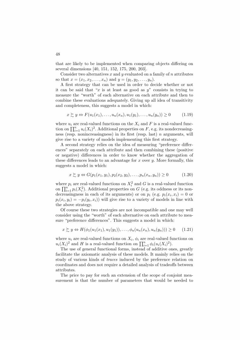
48
that are likely to be implemented when comparing objects differing onseveral dimensions [40, 151, 152, 175, 200, 203].
Consider two alternatives x and y evaluated on a family of n attributesso that x = (x1, x2, . . . , xn) and y = (y1, y2, . . . , yn).
A first strategy that can be used in order to decide whether or notit can be said that “x is at least as good as y” consists in trying tomeasure the “worth” of each alternative on each attribute and then tocombine these evaluations adequately. Giving up all idea of transitivityand completeness, this suggests a model in which:
x % y ⇔ F (u1(x1), . . . , un(xn), u1(y1), . . . , un(yn)) ≥ 0 (1.19)
where ui are real-valued functions on the Xi and F is a real-valued func-tion on
∏ni=1 ui(Xi)
2. Additional properties on F , e.g. its nondecreasing-ness (resp. nonincreasingness) in its first (resp. last) n arguments, willgive rise to a variety of models implementing this first strategy.
A second strategy relies on the idea of measuring “preference differ-ences” separately on each attribute and then combining these (positiveor negative) differences in order to know whether the aggregation ofthese differences leads to an advantage for x over y. More formally, thissuggests a model in which:
x % y ⇔ G(p1(x1, y1), p2(x2, y2), . . . , pn(xn, yn)) ≥ 0 (1.20)
where pi are real-valued functions on X2i and G is a real-valued function
on∏n
i=1 pi(X2i ). Additional properties on G (e.g. its oddness or its non-
decreasingness in each of its arguments) or on pi (e.g. pi(xi, xi) = 0 orpi(xi, yi) = −pi(yi, xi)) will give rise to a variety of models in line withthe above strategy.
Of course these two strategies are not incompatible and one may wellconsider using the “worth” of each alternative on each attribute to mea-sure “preference differences”. This suggests a model in which:
x % y ⇔ H(φ1(u1(x1), u1(y1)), . . . , φn(un(xn), un(yn))) ≥ 0 (1.21)
where ui are real-valued functions on Xi, φi are real-valued functions onui(Xi)
2 and H is a real-valued function on∏n
i=1 φi(ui(Xi)2).
The use of general functional forms, instead of additive ones, greatlyfacilitate the axiomatic analysis of these models. It mainly relies on thestudy of various kinds of traces induced by the preference relation oncoordinates and does not require a detailed analysis of tradeoffs betweenattributes.
The price to pay for such an extension of the scope of conjoint mea-surement is that the number of parameters that would be needed to
Acknowledgements 49
assess such models is quite high. Furthermore, none of them is likelyto possess any remarkable uniqueness properties. Therefore, althoughproofs are constructive, these results will not give direct hints on how todevise assessment procedures. The general idea here is to use numericalrepresentations as guidelines to understand the consequences of a limitednumber of cancellation conditions, without imposing any transitivity orcompleteness requirement on the preference relation and any structuralassumptions on the set of objects. Such models have proved useful to:
understand the ordinal character of some aggregation models pro-posed in the literature [170, 172], known as the “outranking meth-ods” (see Chapters XXX of this Volume) as shown in [28],
understand the links between aggregation models aiming at en-riching a dominance relation and more traditional conjoint mea-surement approaches [30],
to include in a classical conjoint measurement framework, noncom-pensatory preferences in the sense of [22, 33, 55, 60, 61] as shownin [28, 32, 99].
Acknowledgments
We thank two anonymous referees for their very helpful comments andsuggestions. Part of this work was accomplished while Denis Bouyssouwas visiting the Service de Mathematique de la Gestion at the UniversiteLibre de Bruxelles (Brussels, Belgium). The warm hospitality of the Ser-vice de Mathematique de la Gestion, the support of the Belgian FondsNational de la Recherche Scientistic and the Brussels-Capital Regionthrough a “Research in Brussels” action grant are gratefully acknowl-edged. Many Figures in this text were inspired by the ones drawn byChristophe Gonzales in [86].

References
[1] E. W. Adams. Elements of a theory of inexact measurement. Philosophy ofScience, 32:205–228, 1965.
[2] E. W. Adams and R. F. Fagot. A model of riskless choice. Behavioral Science,4:1–10, 1959.
[3] L. Adelman, P. J. Sticha, and M. L. Donnell. An experimental investigationof the relative effectiveness of two techniques for structuring multiattributedhierarchies. Organizational Behavior and Human Decision Processes, 37:188–196, 1986.
[4] F. Aleskerov and B. Monjardet. Utility Maximization, Choice and Preference.Springer Verlag, Heidelberg, 2002.
[5] A. B. Atkinson. On the measurement of inequality. Journal of EconomicTheory, 2:244–263, 1970.
[6] C. A. Bana e Costa. The use of multi-criteria decision analysis to support thesearch for less conflicting policy options in a multi-actor context: Case study.Journal of Multi-Criteria Decision Analysis, 10(2):111–125, 2001.
[7] C. A. Bana e Costa, E. C. Correa, J.-M. De Corte, and J.-C. Vansnick. Fa-cilitating bid evaluation in public call for tenders: A socio-technical approach.Omega, 30(3):227–242, April 2002.
[8] C. A. Bana e Costa, M. L. Costa-Lobo, I. A. J. Ramos, and J.-C. Vansnick.Multicriteria approach for strategic town planning: The case of Barcelos. InD. Bouyssou, E. Jacquet-Lagreze, P. Perny, R. SÃlowinski, D. Vanderpooten,and Ph. Vincke, editors, Aiding Decisions with Multiple Criteria: Essays inHonour of Bernard Roy, pages 429–456. Kluwer, Dordrecht, 2002.
[9] C. A. Bana e Costa, L. Ensslin, E. C. Correa, and J.-C. Vansnick. Decisionsupport systems in action: Integrated application in a multicriteria decissionaid process. European Journal of Operational Research, 113(2):315–335, March1999.
[10] C. A. Bana e Costa, F. Nunes da Silva, and J.-C. Vansnick. Conflict dissolutionin the public sector: A case-study. European Journal of Operational Research,130(2):388–401, April 2001.
[11] C. A. Bana e Costa and R. C. Oliveira. Assigning priorities for maintenanceand repair and refurbishment in managing a municipal housing stock. EuropeanJournal of Operational Research, 138:380–91, 2002.
51
52
[12] C. A. Bana e Costa and J.-C. Vansnick. MACBETH – An interactive path to-wards the construction of cardinal value functions. International Transactionsin Operational Research, 1:489–500, 1994.
[13] A. F. Beardon, J. C. Candeal, G. Herden, E. Indurain, and G. B. Mehta.The non-existence of a utility function and the structure of non-representatblepreference relations. Journal of Mathematical Economics, 37:17–38, 2002.
[14] D. E. Bell. Multilinear representations for ordinal utility functions. Journal ofMathematical Psychology, 31:44–59, 1987.
[15] V. Belton, F. Ackermann, and I. Shepherd. Integrated support from problemstructuring through alternative evaluation using COPE and V•I•S•A. Journalof Multi-Criteria Decision Analysis, 6:115–130, 1997.
[16] V. Belton and T. Stewart. Multiple Criteria Decision Analysis: An IntegratedApproach. Kluwer, Dordrecht, 2001.
[17] E. Ben-Porath and I. Gilboa. Linear measures, the Gini index and the income-equality tradeoff. Journal of Economic Theory, 64:443–467, 1994.
[18] E. Ben-Porath, I. Gilboa, and D. Schmeidler. On the measurement of inequalityunder uncertainty. Journal of Economic Theory, 75:194–204, 1997.
[19] M. Beuthe and G. Scannella. Applications comparees des methodes d’analysemulticritere UTA. RAIRO Recherche Operationnelle / Operations Research,30(3):293–315, 1996.
[20] M. Beuthe and G. Scannella. Comparative analysis of UTA multicriteria meth-ods. European Journal of Operational Research, 130(2):246–262, 2001.
[21] C. Blackorby, D. Primont, and R. Russell. Duality, separability, and functionalstructure: Theory and economic applications. North-Holland, New York, 1978.
[22] D. Bouyssou. Some remarks on the notion of compensation in MCDM. Euro-pean Journal of Operational Research, 26:150–160, 1986.
[23] D. Bouyssou. Modelling inaccurate determination, uncertainty, imprecision us-ing multiple criteria. In A. G. Lockett and G. Islei, editors, Improving DecisionMaking in Organisations, pages 78–87. Springer Verlag, Heidelberg, 1989.
[24] D. Bouyssou. Builing criteria: A prerequisite for MCDA. In C. A. Bana eCosta, editor, Readings in Multiple Criteria Decision Aid, pages 58–81, Berlin,1990. Springer Verlag.
[25] D. Bouyssou. Outranking methods. In C. A. Floudas and P. M. Pardalos,editors, Encyclopedia of optimization, volume 4, pages 249–255. Kluwer, 2001.
[26] D. Bouyssou, S. Greco, B. Matarazzo, M. Pirlot, and R. SÃlowinski. Characteri-zation of ‘max’, ‘min’ and ‘order statistics’ multicriteria aggregation functions.Communication to IFORS’2002, 8 – 12 July, 2002, Edinburgh, U.K., July 2002.
[27] D. Bouyssou, Th. Marchant, M. Pirlot, P. Perny, A. Tsoukias, and Ph. Vincke.Evaluation and Decision models: A critical perspective. Kluwer, Dordrecht,2000.
[28] D. Bouyssou and M. Pirlot. A characterization of strict concordance relations.In D. Bouyssou, E. Jacquet-Lagreze, P. Perny, R. SÃlowinski, D. Vanderpooten,
References 53
and Ph. Vincke, editors, Aiding Decisions with Multiple Criteria: Essays inHonour of Bernard Roy, pages 121–145. Kluwer, Dordrecht, 2002.
[29] D. Bouyssou and M. Pirlot. Nontransitive decomposable conjoint measure-ment. Journal of Mathematical Psychology, 46:677–703, 2002.
[30] D. Bouyssou and M. Pirlot. Preferences for multiattributed alternatives:Traces, dominance, and numerical representations. Working Paper, LAM-SADE, Universite Paris-Dauphine, submitted, 2002.
[31] D. Bouyssou and M. Pirlot. ‘Additive difference’ models without additivityand subtractivity. Working Paper, LAMSADE, Universite Paris-Dauphine,submitted, 2003.
[32] D. Bouyssou and M. Pirlot. A characterization of concordance relations. Work-ing Paper, LAMSADE, Universite Paris-Dauphine, 2003.
[33] D. Bouyssou and J.-C. Vansnick. Noncompensatory and generalized noncom-pensatory preference structures. Theory and Decision, 21:251–266, 1986.
[34] D. S. Briges and G. B. Mehta. Representations of preference orderings. SpringerVerlag, Berlin, 1995.
[35] J. D. Carroll and P. E. Green. Psychometric methods in marketing research.Part 1. Conjoint analysis. Journal of Marketing Research, 32:385–391, 1995.
[36] A. Charnes and W. W. Cooper. Management Models and Industrial Applica-tions of Linear Programming. Wiley, New York, 1961.
[37] A. Chateauneuf and P. P. Wakker. From local to global additive representation.Journal of Mathematical Economics, 22(6):523–545, 1993.
[38] J.-C. Cosset, Y. Siskos, and C. Zopounidis. The evaluation of country risk: Adecision support approach. Global Finance Journal, 3:79–95, 1992.
[39] M. A. Croon. The axiomatization of additive difference models for prefer-ence judgements. In E. Degreef and G. van Buggenhaut, editors, Trends inMathematical Psychology, pages 193–227, Amsterdam, 1984. North-Holland.
[40] V. Dahlstrand and H. Montgomery. Information search and evaluation pro-cesses in decision-making: A computer-based process tracking study. ActaPsychologica, 56:113–123, 1984.
[41] P. de Donder, M. Le Breton, and M. Truchon. Choosing from a weightedtournament. Mathematical Social Sciences, 40:85–109, 2000.
[42] G. Debreu. Representation of a preference ordering by a numerical function.In R. Thrall, C. H. Coombs, and R. Davies, editors, Decision Processes, pages159–175, New York, 1954. Wiley.
[43] G. Debreu. Theory of value: An axiomatic analysis of economic equilibrium.John Wiley & Sons, New York, 1959.
[44] G. Debreu. Topological methods in cardinal utility theory. In K. J. Arrow,S. Karlin, and P. Suppes, editors, Mathematical methods in the Social Sciences,pages 16–26. Stanford University Press, Stanford, 1960.

54
[45] G. Debreu. Continuity properties of Paretian utility. International EconomicReview, 5(3):285–293, September 1964.
[46] Ph. Delquie. Inconsistent trade-offs between attributes: New evidence in pref-erence assessment biases. Management Science, 39(11):1382–1395, November1993.
[47] A. I. Dimitras, C. Zopounidis, and C. Hurson. Assessing financial risks usinga multicriteria sorting procedure: The case of country risk assessment. Foun-dations of Computing and Decision Sciences, 29:97–109, 2001.
[48] M. Doumpos, S. H. Zanakis, and C. Zopounidis. Multicriteria preference dis-aggregation for classification problems with an application to global investingrisk. Decision Sciences, 32(2):333–385, 2001.
[49] D. Dubois, J.-L. Marichal, H. Prade, M. Roubens, and R. Sabbadin. The useof the discrete Sugeno integral in decision-making: A survey. InternationalJournal of Uncertainty, Fuzziness and Knowledge-Based Systems, 9(5):539–561, 2001.
[50] J. S. Dyer and R. K. Sarin. Measurable multiattribute value functions. Oper-ations Research, 27:810–822, 1979.
[51] W. Edwards. Social utilities. Engineering Economist, 6:119–129, 1971.
[52] W. Edwards. How to use multiattribute utility measurement for social decisionmaking. IEEE Transactions on Systems, Man and Cybernetics, 7(5):326–340,1977.
[53] W. Edwards and F. Hutton Barron. SMART and SMARTER: Improved simplemethods for multiattribute utility measurement. Organizational Behavior andHuman Decision Processes, 60:306–325, 1994.
[54] J.-C. Falmagne. On a class of probabilistic conjoint measurement models: Somediagnostic properties. Journal of Mathematical Psychology, 19(2):73–88, 1979.
[55] H. Fargier and P. Perny. Modelisation des preferences par une regle de concor-dance generalisee. In A. Colorni, M. Paruccini, and B. Roy, editors, A-MCD-A,Aide Multicritere a la Decision/Multiple Criteria Decision Aid, pages 99–115.European Commission, Joint Research Centre, 2001.
[56] Final report of the British Association for the Advancement of Science. 2:331–349, 1940.
[57] P. C. Fishburn. Intransitive indifference in preference theory: A survey. Oper-ations Research, 18(2):207–228, 1970.
[58] P. C. Fishburn. Utility theory for decision-making. Wiley, New York, 1970.
[59] P. C. Fishburn. Lexicographic orders, utilities and decision rules: A survey.Management Science, 20(11):1442–1471, 1974.
[60] P. C. Fishburn. Axioms for lexicographic preferences. Review of EconomicStudies, 42:415–419, 1975.
[61] P. C. Fishburn. Noncompensatory preferences. Synthese, 33:393–403, 1976.
References 55
[62] P. C. Fishburn. Condorcet social choice functions. SIAM Journal on AppliedMathematics, 33:469–489, 1977.
[63] P. C. Fishburn. A survey of multiattribute/multicriteria evaluation theories.In S. Zionts, editor, Multicriteria problem solving, pages 181–224. SpringerVerlag, Berlin, 1978.
[64] P. C. Fishburn. Lexicographic additive differences. Journal of MathematicalPsychology, 21:191–218, 1980.
[65] P. C. Fishburn. Nontransitive measurable utility. Journal of MathematicalPsychology, 26:31–67, 1982.
[66] P. C. Fishburn. Interval orders and intervals graphs. Wiley, New York, 1985.
[67] P. C. Fishburn. Nonlinear preference and utility theory. Johns Hopkins Uni-versity Press, Baltimore, 1988.
[68] P. C. Fishburn. Normative theories of decision making under risk and underuncertainty. In Nonconventional preference relations in decision making, pages1–21. Springer, Berlin, 1988.
[69] P. C. Fishburn. Additive non-transitive preferences. Economic Letters, 34:317–321, 1990.
[70] P. C. Fishburn. Continuous nontransitive additive conjoint measurement.Mathematical Social Sciences, 20:165–193, 1990.
[71] P. C. Fishburn. Skew symmetric additive utility with finite states. Mathemat-ical Social Sciences, 19:103–115, 1990.
[72] P. C. Fishburn. Nontransitive additive conjoint measurement. Journal ofMathematical Psychology, 35:1–40, 1991.
[73] P. C. Fishburn. Nontransitive preferences in decision theory. Journal of Riskand Uncertainty, 4:113–134, 1991.
[74] P. C. Fishburn. Additive differences and simple preference comparisons. Jour-nal of Mathematical Psychology, 36:21–31, 1992.
[75] P. C. Fishburn. A general axiomatization of additive measurement with appli-cations. Naval Research Logistics, 39(6):741–755, 1992.
[76] P. C. Fishburn. On nonstandard nontransitive additive utility. Journal ofEconomic Theory, 56:426–433, 1992.
[77] P. C. Fishburn. Finite linear qualitative probability. Journal of MathematicalPsychology, 40:21–31, 1996.
[78] P. C. Fishburn. Cancellation conditions for multiattribute preferences on finitesets. In M. H. Karwan, J. Spronk, and J. Wallenius, editors, Essays in DecisionMaking, pages 157–167, Berlin, 1997. Springer Verlag.
[79] S. French. Decision theory – An introduction to the mathematics of rationality.Ellis Horwood, London, 1993.
[80] D. G. Fryback and R. L. Keeney. Constructing a complex judgmental model:An index of trauma severity. Management Science, 29:869–883., 1983.

56
[81] G. Furkhen and M. K. Richter. Additive utility. Economic Theory, 1:83–105,1991.
[82] G. Furkhen and M. K. Richter. Polynomial utility. Economic Theory, 1:231–249, 1991.
[83] D. Gale. The theory of linear economic models. McGraw-Hill, New York, 1960.
[84] I. Gilboa and R. Lapson. Aggregation of semiorders: Intransitive indifferencemakes a difference. Economic Theory, 5:109–126, 1995.
[85] Ch. Gonzales. Additive utilities when some components are solvable and othersnot. Journal of Mathematical Psychology, 40:141–151, 1996.
[86] Ch. Gonzales. Utilites additives : Existence et construction. These de doctorat,Universite Paris 6, Paris, France, 1996.
[87] Ch. Gonzales. Two factor additive conjoint measurement with one solvablecomponent. Journal of Mathematical Psychology, 44:285–309, 2000.
[88] Ch. Gonzales. Additive utility without restricted solvavibility on every com-ponent. Journal of Mathematical Psychology, 47:47–65, 2003.
[89] W. M. Gorman. The structure of utility functions. Review of Economic Studies,XXXV:367–390, 1968.
[90] M. Grabisch. The application of fuzzy integrals to multicriteria decision mak-ing. European Journal of Operational Research, 89:445–456, 1996.
[91] M. Grabisch. Fuzzy integral as a flexible and interpretable tool of aggregation.In Aggregation and fusion of imperfect information, pages 51–72. Physica, Hei-delberg, 1998.
[92] M. Grabisch, Ch. Labreuche, and J.-C. Vansnick. On the extension of pseudo-boolean functions for the aggregation of interacting criteria. European Journalof Operational Research, 148(1):28–47, 2003.
[93] M. Grabisch, S. A. Orlovski, and R. R. Yager. Fuzzy aggregation of numericalpreferences. In R. SÃlowinski, editor, Fuzzy sets in decision analysis, operationsresearch and statistics, pages 31–68. Kluwer, Boston, MA, 1998.
[94] M. Grabisch and P. Perny. Agregation multicritere. In B. Bouchon-Meunierand C. Marsala, editors, Logique floue, Principes, Aide a la decision, IC2, pages82–120. Hermes, 2002.
[95] M. Grabisch and M. Roubens. Application of the Choquet integral in multicri-teria decision making. In M. Grabisch, T. Murofushi, and M. Sugeno, editors,Fuzzy measures and integrals, pages 348–374. Physica Verlag, Heidelberg, 2000.
[96] N. Grassin. Constructing criteria population for the comparison of differentoptions of high voltage line routes. European Journal of Operational Research,26:42–47, 1886.
[97] S. Greco, B. Matarazzo, and R. SÃlowinski. Rough approximation of a preferencerelation by dominance relations. European Journal of Operational Research,117:63–83, 1999.
References 57
[98] S. Greco, B. Matarazzo, and R. SÃlowinski. The use of rough sets and fuzzy setsin MCDM. In T. Gal, T. Hanne, and T. Stewart, editors, Multicriteria decisionmaking, Advances in mcdm models, algorithms, theory and applications, pages14.1–14.59, Dordrecht, 1999. Kluwer.
[99] S. Greco, B. Matarazzo, and R. SÃlowinski. Axiomatic basis of noncompen-satoty preferences. Communication to FUR X (Foundations of Utility andRisk Theory), 30 May–2 June, Torino, Italy, 2001.
[100] S. Greco, B. Matarazzo, and R. SÃlowinski. Conjoint measurement and roughset approach for multicriteria sorting problems in presence of ordinal criteria.In A. Colorni, M. Paruccini, and B. Roy, editors, A-MCD-A, Aide Multicriterea la Decision/Multiple Criteria Decision Aid, pages 117–144. European Com-mission, Joint Research Centre, 2001.
[101] S. Greco, B. Matarazzo, and R. SÃlowinski. Rough sets theory for multicriteriadecision analysis. European Journal of Operational Research, 129:1–47, 2001.
[102] S. Greco, B. Matarazzo, and R. SÃlowinski. Preference representation by meansof conjoint measurement and decision rule model. In D. Bouyssou, E. Jacquet-Lagreze, P. Perny, R. SÃl owinski, D. Vanderpooten, and Ph. Vincke, editors,Aiding Decisions with Multiple Criteria: Essays in Honour of Bernard Roy,pages 263–313. Kluwer, Dordrecht, 2002.
[103] P. E. Green and V. Srinivasan. Conjoint analysis in consumer research: Issuesand outlook. Journal of Consumer Research, 5:103–152, 1978.
[104] P. E. Green, D. S. Tull, and G. Albaum. Research for marketing decisions.Englewood Cliffs, 1988.
[105] E. Grigoroudis, Y. Siskos, and O. Saurais. TELOS: A customer satisfactionevaluation software. Computers and Operations Research, 27(7–8):799–817,2000.
[106] J. Guild. Part III of Quantitative estimation of sensory events. Interim report,British Academy for the Advancement of Science, 1936. pp. 296–328.
[107] F. Gul. Savage’s theorem with a finite number of states. Journal of EconomicTheory, 57:99–110, 1992.
[108] G. Iverson and J.-C. Falmagne. Statistical issues in measurement. Mathemat-ical Social Sciences, 10:131–153, 1985.
[109] E. Jacquet-Lagreze. Interactive assessment of preferences using holistic judg-ments. The PREFCALC system. In C. A. Bana e Costa, editor, Readings inmultiple criteria decision aid, pages 335–350. Springer Verlag, Berlin, 1990.
[110] E. Jacquet-Lagreze. An application of the UTA discriminant model for theevaluation of R&D projects. In P. Pardalos, Y. Siskos, and C. Zopounidis,editors, Advances in Multicriteria Analysis, pages 203–211. Kluwer AcademicPublishers, Dordrecht, 1995.
[111] E. Jacquet-Lagreze and J. Siskos. Assessing a set of additive utility functionsfor multicriteria decision making: The UTA method. European Journal ofOperational Research, 10:151–164, 1982.

58
[112] J.-Y. Jaffray. Existence, proprietes de continuite, additivite de fonctionsd’utilite sur un espace partiellement ou totalement ordonne. These de doc-torat d’etat, Universite Paris 6, Paris, France, 1974.
[113] J.-Y. Jaffray. On the extension of additive utilities to infinite sets. Journal ofMathematical Psychology, 11:431–452, 1974.
[114] R. M. Johnson. Trade-off analysis of consumer values. Journal of MarketingResearch, 11:121–127, 1974.
[115] E. Karni and Z. Safra. The hexagon condition and additive representation fortwo dimensions: An algebraic approach. Journal of Mathematical Psychology,42:393–399, 1998.
[116] R. L. Keeney. Measurement scales for quantifying attributes. Behavioral Sci-ence, 26:29–36, 1981.
[117] R. L. Keeney. Building models of values. European Journal of OperationalResesearch, 37(2):149–157, 1988.
[118] R. L. Keeney. Structuring objectives for problems of public interest. OperationsResearch, 36:396–405, 1988.
[119] R. L. Keeney. Value-focused thinking. Harvard University Press, Cambridge,MA., 1992.
[120] R. L. Keeney, J. S. Hammond, and H. Raiffa. Smart choices: A guide to makingbetter decisions. Harvard University Press, Boston, 1999.
[121] R. L. Keeney and H. Raiffa. Decisions with multiple objectives: Preferencesand value tradeoffs. Wiley, New York, 1976.
[122] R. L. Keeney and G. A. Robillard. Assessing and evaluating environ-mentalimpacts at proposed nuclear power plant sites. Journal of Environmental Eco-nomics and Management, 4:153–166, 1977.
[123] V. Kobberling. Strenth of preference and cardinal utility. Working paper,University of Maastricht, Maastricht, June 2002.
[124] V. Kobberling. Comment on: Edi Karni & Zvi Safra (1998) The hexagon con-dition and additive representation for two dimensions: An algebraic approach.Journal of Mathematical Psychology, 47(3):370, 2003.
[125] T. C. Koopmans. Stationary ordinal utility and impatience. Econometrica,28:287–309, 1960.
[126] T. C. Koopmans. Representation of prefernce orderings over time. In C. B.McGuire and R. Radner, editors, Decision and Organization, pages 57–100.Noth-Holland, Amsterdam, 1972.
[127] D. H. Krantz. Conjoint measurement: The Luce-Tukey axiomatization andsome extensions. Journal of Mathematical Psychology, 1:248–277, 1964.
[128] D. H. Krantz. Extensive measurement in semiorders. Philosophy of Science,34:348–362, 1967.
References 59
[129] D. H. Krantz, R. D. Luce, P. Suppes, and A. Tversky. Foundations of mea-surement, vol. 1: Additive and polynomial representations. Academic Press,New York, 1971.
[130] G. Laffond, J.-F. Laslier, and M. Le Breton. Condorcet choice correspondences:A set-theoretical comparison. Mathematical Social Sciences, 30:23–36, 1995.
[131] J.-F. Laslier. Tournament solutions and majority voting. Springer Verlag,Berlin, 1997.
[132] J. Louviere. Analyzing Decision Making: Metric Conjoint Analysis. Sage, Park,CA, 1988.
[133] R. D. Luce. Semiorders and a theory of utility discrimination. Econometrica,24:178–191, 1956.
[134] R. D. Luce. Three axiom systems for additive semiordered structures. SIAMJournal of Applied Mathematics, 25:41–53, 1973.
[135] R. D. Luce. Conjoint measurement: A brief survey. In David E. Bell, Ralph L.Keeney, and Howard Raiffa, editors, Conflicting objectives in decisions, pages148–171. Wiley, New York, 1977.
[136] R. D. Luce. Lexicographic tradeoff structures. Theory and Decision, 9:187–193,1978.
[137] R. D. Luce. Utility of gains and losses: Measurement-theoretical and experi-mental approaches. Lawrence Erlbaum Publishers, Mahwah, New Jersey, 2000.
[138] R. D. Luce and M. Cohen. Factorizable automorphisms in solvable conjointstructures. I. Journal of Pure and Applied Algebra, 27(3):225–261, 1983.
[139] R. D. Luce, D. H. Krantz, P. Suppes, and A. Tversky. Foundations of measure-ment, vol. 3: Representation, axiomatisation and invariance. Academic Press,New York, 1990.
[140] R. D. Luce and A. A. J. Marley. Extensive measurement when concatenationis restricted. In S. Morgenbessser, P. Suppes, and M. G. White, editors, Phi-losophy, science and method: Essays in honor of Ernest Nagel, pages 235–249.St. Martin’s Press, New York, 1969.
[141] R. D. Luce and J. W. Tukey. Simultaneous conjoint measurement: A new typeof fundamental measurement. Journal of Mathematical Psychology, 1:1–27,1964.
[142] A. Maas and P. P. Wakker. Additive conjoint measurement for multiattributeutility. Journal of Mathematical Psychology, 38:86–101, 1994.
[143] J.-L. Marichal. An axiomatic approach of the discrete Choquet integral as atool to aggregate interacting criteria. IEEE Transactions on Fuzzy Systems,8, 2000.
[144] J.-L. Marichal. On Choquet and Sugeno integrals as aggregation functions.In M. Grabisch, T. Murofushi, and M. Sugeno, editors, Fuzzy measures andintegrals, pages 247–272. Physica Verlag, Heidelberg, 2000.
[145] J.-L. Marichal. On Sugeno integralsas an aggregation function. Fuzzy Sets andSystems, 114, 2000.
60
[146] J.-L. Marichal and M. Roubens. Determination of weights of interacting crite-ria from a reference set. European Journal of Operational Research, 124:641–50,2000.
[147] K. O. May. Intransitivity, utility and the aggregation of preference patterns.Econometrica, 22:1–13, 1954.
[148] G. Mihelis, E. Grigoroudis, Y. Siskos, Y. Politis, and Y. Malandrakis. Customersatisfaction measurement in the private bank sector. European Journal ofOperational Research, 130(2):347–360, April 2001.
[149] N. R. Miller. Graph theoretical approaches to the theory of voting. AmericanJournal of Political Science, 21:769–803, 1977.
[150] J. Miyamoto and P. P. Wakker. Multiattribure utility theory without expectedutility foundations. Operations Research, 44(2):313–326, 1996.
[151] H. Montgomery. A study of intransitive preferences using a think aloud proce-dure. In H. Jungerman and G. de Zeeuw, editors, Decision-making and Changein Human Affairs, pages 347–362, Dordrecht, 1977. D. Reidel.
[152] H. Montgomery and O. Svenson. On decision rules and information processingstrategies for choice among multiattribute alternatives. Scandinavian Journalof Psychology, 17:283–291, 1976.
[153] Y. Nakamura. Lexicographic additivity for multi-attribute preferences on finitesets. Theory and Decision, 42:1–19, 1997.
[154] Y. Nakamura. Additive utility on densely ordered sets. Journal of Mathemat-ical Psychology, 46:515–530, 2002.
[155] L. Narens. Abstract measurement theory. MIT press, Cambridge, Mass., 1985.
[156] L. Narens and R. D. Luce. The algebra of measurement. Journal of Pure andApplied Algebra, 8(2):197–233, 1976.
[157] A. Ostanello. Action evaluation and action structuring – Different decision aidsituations reviewed through two actual cases. In C. A. Bana e Costa, editor,Readings in multiple criteria decision aid, pages 36–57. Springer Verlag, Berlin,1990.
[158] J. E. Peris and B. Subiza. Condorcet choice correspondences for weak tourna-ments. Social Choice and Welfare, 16:217–231, 1999.
[159] J. Pfanzagl. Theory of measurement. Physica Verlag, Wurzburg, 2nd revisededition edition, 1971.
[160] M. Pirlot and Ph. Vincke. Lexicographic aggregation of semiorders. Journalof Multicriteria Decision Analysis, 1:47–58, 1992.
[161] M. Pirlot and Ph. Vincke. Semiorders. Properties, representations, applica-tions. Kluwer, Dordrecht, 1997.
[162] J.-Ch. Pomerol and S. Barba-Romero. Multicriterion Decision in Management,Principles and Practice. Kluwer, Dordrecht, 2000.
References 61
[163] M. Poyhonen, H. Vrolijk, and R. P. Hamalainen. Behavioral and procedu-ral consequences of structural variations in value trees. European Journal ofOperational Research, 134(1):216–227, October 2001.
[164] H. Raiffa. Decision analysis – Introductory lectures on choices under uncer-tainty. Addison-Wesley, Reading, Mass., 1968.
[165] H. Raiffa. Preference for multi-attributed alternatives. RAND Memorandum,RM-5868-DOT/RC, December 1968.
[166] M. K. Richter. Rational choice and polynomial measurement theory. Journalof Mathematical Psychology, 12:99–113, 1975.
[167] F. S. Roberts. Measurement theory with applications to decision making, utilityand the social sciences. Addison-Wesley, Reading, 1979.
[168] F. S. Roberts and R. D. Luce. Axiomatic thermodynamics and extensivemeasurement. Synthese, 18:311–326, 1968.
[169] M. Roubens and Ph. Vincke. Preference modelling. Springer Verlag, Berlin,1985.
[170] B. Roy. Classement et choix en presence de points de vue multiples (la methodeelectre). RIRO, 2:57–75, 1968.
[171] B. Roy. Main sources of inaccurate determination, uncertainty and imprecisionin decision models. Mathematical and Computer Modelling, 12(10–11):1245–1254, 1989.
[172] B. Roy. The outranking approach and the foundations of electre methods.Theory and Decision, 31:49–73, 1991.
[173] B. Roy. Multicriteria methodology for decision aiding. Kluwer, Dordrecht, 1996.Original version in French “Methodologie multicritere d’aide a la decision”,Economica, Paris, 1985.
[174] B. Roy and D. Bouyssou. Aide multicritere a la decision : methodes et cas.Economica, Paris, 1993.
[175] J. E. Russo and B. A. Dosher. Strategies for multiattribute binary choice.Journal of Experimental Psychology: Learning, Memory and Cognition, 9:676–696, 1983.
[176] D. G. Saari. Connecting and resolving Sen’s and Arrow’s theorems. SocialChoice and Welfare, 15:239–261, 1998.
[177] L. J. Savage. The Foundations of Statistics. John Wiley and Sons, New York,1954.
[178] T. Schwartz. The logic of collectice choice. Columbia University Press, 1986.
[179] D. Scott. Measurement structures and linear inequalities. Journal of Mathe-matical Psychology, 1:233–247, 1964.
[180] D. Scott and P. Suppes. Foundational aspects of theories of measurement.Journal of Symbolic Logic, 23:113–128, 1958.
[181] U. Segal. A sufficient condition for additively separable functions. Journal ofMathematical Economics, 23:295–303, 1994.
62
[182] U. Segal and J. Sobel. Min, Max and Sum. Journal of Economic Theory,106:126–150, 2002.
[183] A. K. Sen. Social choice theory. In K. J. Arrow and M. D. Intriligator, edi-tors, Handbook of mathematical economics, volume 3, pages 1073–1181. North-Holland, Amsterdam, 1986.
[184] L. Shapiro. Conditions for expected uility maximization. Annals of Statistics,7:1288–1302, 1979.
[185] Y. Siskos. Evaluating a system of furniture retail outlets using an interactiveordinal regression model. European Journal of Operational Research, 23:179–193, 1986.
[186] Y. Siskos and D. K. Despotis. A DSS oriented method for multiobjective linearprogramming problems. Decision Support Systems, 5(1):47–56, 1989.
[187] Y. Siskos, D. K. Despotis, and M. Ghediri. Multiobjective modelling for re-gional agricultural planning: Case study in Tunisia. European Journal of Op-erational Research, 77(3):375–391, 1993.
[188] Y. Siskos, E. Grigoroudis, C. Zopounidis, and O. Saurais. Measuring cus-tomer satisfaction using a collective preference disaggregation model. Journalof Global Optimization, 12(2):175–195, 1998.
[189] Y. Siskos, N. F. Matsatsinis, and G. Baourakis. Multicriteria analysis in agri-cultural marketing: The case of French olive oil market. European Journal ofOperational Research, 130(2):315–331, April 2001.
[190] Y. Siskos, A. Spyridakos, and D. Yannacopoulos. Using artificial intelligenceand visual techniques into preference disaggregation analysis: The MIIDASsystem. European Journal of Operational Research, 113(2):281–299, March1999.
[191] Y. Siskos and D. Yannacopoulos. UTASTAR, An ordinal regression method forbuilding additive value functions. Investigacao Operacional, 5(1):39–53, 1985.
[192] Y. Siskos and C. Zopounidis. The evaluation of venture capital investmentactivity: An interactive assessment. European Journal of Operational Research,31(3):304–313, 1987.
[193] H. J. Skala. Non-Archimedean Utility Theory. Kluwer, Dordrecht, 1975.
[194] J. Sounderpandian. Value functions when decision criteria are not totallysubstitutable. Operations Research, 39:592–600, 1991.
[195] A. Spyridakos, Y. Siskos, D. Yannacopoulos, and A. Skouris. Multicriteria jobevaluation for large organizations. European Journal of Operational Research,130(2):375–387, April 2001.
[196] T. Stewart. An interactive multiple objective linear programming methodbased on piecewise linear additive value functions. IEEE Transactions onSystems, Man, and Cybernetics, SMC-17(5):799–805, 1987.
[197] W. G. Stillwell, D. von Winterfeldt, and R. S. John. Comparing hierarchi-cal and nonhierarchical weighting methods for eliciting multiattribute valuemodels. Management Science, 33:442–50, 1987.
References 63
[198] P. Suppes, D. H. Krantz, R. D. Luce, and A. Tversky. Foundations of mea-surement, vol. 2: Geometrical, threshold, and probabilistic representations. Aca-demic Press, New York, 1989.
[199] P. Suppes and M. Winet. An axiomatization of utility based on the notion ofutility difference. Management Science, 1:259–270, 1955.
[200] O. Svenson. Process description of decision making. Organizational Behaviorand Human Performance, 23:86–112, 1979.
[201] R. J. Titiev. Measurement structures in classes that are not universally ax-iomatizable. Journal of Mathematical Psychology, 9:200–205, 1972.
[202] A. Tversky. A general theory of polynomial conjoint measurement. Journal ofMathematical Psychology, 4:1–20, 1967.
[203] A. Tversky. Intransitivity of preferences. Psychological Review, 76:31–48, 1969.
[204] Ph. Vincke. Multi-criteria decision aid. Wiley, New York, 1992. Originalversion in French “L’Aide Multicritere a la Decision”, Editions de l’Universitede Bruxelles-Editions Ellipses, Brussels, 1989.
[205] Ph. Vincke. Outranking approach. In T. Gal, T. Stewart, and T. Hanne,editors, Multicriteria decision making, Advances in mcdm models, algorithms,theory and applications, pages 11.1–11.29. Kluwer, 1999.
[206] K. Vind. Independent preferences. Journal of Mathematical Economics,20:119–135, 1991.
[207] J. von Neumann and O. Morgenstern. Theory of games and economic behavior.Wiley, 2nd edition, 1947.
[208] R. von Nitzsch and M. Weber. The effect of attribute ranges on weights in mul-tiattribute utility measurements. Management Science, 39(8):937–943, August1993.
[209] D. von Winterfeldt and W. Edwards. Decision analysis and behavioral research.Cambridge University Press, Cambridge, 1986.
[210] P. P. Wakker. Cardinal coordinate independence for expected utility. Journalof Mathematical Psychology, 28(1):110–117, 1984.
[211] P. P. Wakker. Additive representations of preferences: A new foundation ofdecision analysis. Kluwer, Dordrecht, 1989.
[212] P. P. Wakker. Additive representation for equally spaced structures. Journalof Mathematical Psychology, 35:260–266, 1991.
[213] P. P. Wakker. Additive representations of preferences, A new foundation of de-cision analysis; The algebraic approach. In J.-P. Doignon and J.-C. Falmagne,editors, Mathematical Psychology: Current Developments, pages 71–87, Berlin,1991. Springer Verlag.
[214] P. P. Wakker. Additive representations on rank-ordered sets. I. The algebraicapproach. Journal of Mathematical Psychology, 35(4):501–531, 1991.
[215] P. P. Wakker. Additive representations on rank-ordered sets. II. The topolog-ical approach. Journal of Mathematical Economics, 22(1):1–26, 1993.

64
[216] M. Weber, F. Eisenfuhr, and D. von Winterfeld. The effects of splitting at-tributes on weights in multiattribute utility measurement. Management Sci-ence, 34(4):431–445, 1988.
[217] J. A. Weymark. Generalized Gini inequality indices. Mathematical SocialSciences, 1:409–430, 1981.
[218] U. Wille. Linear measurement models: Axiomatizations and axiomatizability.Journal of Mathematical Psychology, 44:617–650, 2000.
[219] C. Zopounidis and M. Doumpos. Stock evaluation using a preference disag-gregation methodology. Decision Science, 30:313–336, 1999.
[220] C. Zopounidis and M. Doumpos. Building additive utilities for multi-grouphierarchical discrimination: The MHDIS method. Optimization Methods &Software, 14(3):219–240, 2000.
[221] C. Zopounidis and M. Doumpos. PREFDIS: A multicriteria decision supportsystem for sorting decision problems. Computers & Operations Research, 27(7–8):779–797, June 2000.
[222] C. Zopounidis and M. Doumpos. Multicriteria preference disaggregation forclassification problems with an application to global investing risk. DecisionSciences, 32(2):333–385, 2001.
[223] C. Zopounidis and M. Doumpos. A preference disaggregation decision supportsystem for financial classification problems. European Journal of OperationalResearch, 130(2):402–413, April 2001.


![APPLE 7243 4 96895 2 7 THE BEATLES [2-CD]](https://static.fdocuments.net/doc/165x107/622fdc3342bf595bf3701eb3/apple-7243-4-96895-2-7-the-beatles-2-cd.jpg)

![Laboratoire ’Aide à la Décision UMR 7243 lamsade...In Plato, discrete appears more concretely and with more constructive details. In his dialogue T o& (Timaios, [17]), Plato develops](https://static.fdocuments.net/doc/165x107/6135f0bb0ad5d2067647b2a5/laboratoire-aaide-la-dcision-umr-7243-lamsade-in-plato-discrete-appears.jpg)