BAYESIAN HYPERSPECTRAL UNMIXING WITH MULTIVARIATE BETADISTRIBUTIONS

By

DMITRI DRANISHNIKOV

A DISSERTATION PRESENTED TO THE GRADUATE SCHOOLOF THE UNIVERSITY OF FLORIDA IN PARTIAL FULFILLMENT

OF THE REQUIREMENTS FOR THE DEGREE OFDOCTOR OF PHILOSOPHY

UNIVERSITY OF FLORIDA

2014

c© 2014 Dmitri Dranishnikov

2

To my family, for encouraging me to pursue my dreams

3

ACKNOWLEDGMENTS

I would like to thank my advisor, Dr. Paul Gader, for all of his guidance and support

throughout my studies and research. I would also like to thank my committee members,

Dr. Sergei Shabanov, Dr. Anand Rangarajan, Dr. Yuli Rudyak, and Dr. Joseph Wilson,

for all of their help and valuable suggestions.

Thank you as well to my many former and current lab-mates and friends, for

providing valuable criticism of my work. I am particularly grateful to my friends Rin

Azrak, Marie Mendoza, and Diana Petrukhina for encouraging me to research and

to write. Words are not sufficient to express my thanks to Rin Azrak in particular, for

her boundless kindness and inspiration without which this work would not have been

possible.

Above all, thank you to my family, my parents Alex and Anna Dranishnikov, and my

brother Peter Dranishnikov for their love, support, and understanding.

4

TABLE OF CONTENTS

page

ACKNOWLEDGMENTS . . . . . . . . . . . . . . . . . . . . . . . . . . . . . . . . . . 4

LIST OF TABLES . . . . . . . . . . . . . . . . . . . . . . . . . . . . . . . . . . . . . . 7

LIST OF FIGURES . . . . . . . . . . . . . . . . . . . . . . . . . . . . . . . . . . . . . 8

ABSTRACT . . . . . . . . . . . . . . . . . . . . . . . . . . . . . . . . . . . . . . . . . 9

CHAPTER

1 INTRODUCTION . . . . . . . . . . . . . . . . . . . . . . . . . . . . . . . . . . . 10

1.1 Linear Mixing Model . . . . . . . . . . . . . . . . . . . . . . . . . . . . . . 111.2 Normal Compositional Model . . . . . . . . . . . . . . . . . . . . . . . . . 121.3 Statement of Problem . . . . . . . . . . . . . . . . . . . . . . . . . . . . . 131.4 Overview of Research . . . . . . . . . . . . . . . . . . . . . . . . . . . . . 13

2 LITERATURE REVIEW . . . . . . . . . . . . . . . . . . . . . . . . . . . . . . . 16

2.1 Geometric Methods . . . . . . . . . . . . . . . . . . . . . . . . . . . . . . 172.1.1 Pure Pixel Methods . . . . . . . . . . . . . . . . . . . . . . . . . . . 172.1.2 Minimum Volume Based Methods . . . . . . . . . . . . . . . . . . . 20

2.2 Statistical Methods . . . . . . . . . . . . . . . . . . . . . . . . . . . . . . . 222.2.1 Two General Approaches . . . . . . . . . . . . . . . . . . . . . . . 232.2.2 Bayesian Source Separation . . . . . . . . . . . . . . . . . . . . . . 26

2.2.2.1 Dependent component analysis . . . . . . . . . . . . . . 262.2.2.2 Bayesian positive source separation . . . . . . . . . . . . 272.2.2.3 BSS : methods . . . . . . . . . . . . . . . . . . . . . . . . 28

2.2.3 Normal Compositional Model . . . . . . . . . . . . . . . . . . . . . 322.2.3.1 Maximum likelihood for NCM-based models . . . . . . . . 332.2.3.2 Bayesian NCM-based models . . . . . . . . . . . . . . . 342.2.3.3 Summary of NCM-based models . . . . . . . . . . . . . . 39

2.3 Evaluation Strategies . . . . . . . . . . . . . . . . . . . . . . . . . . . . . 402.3.1 Synthetic Data . . . . . . . . . . . . . . . . . . . . . . . . . . . . . 402.3.2 Remotely Sensed Images . . . . . . . . . . . . . . . . . . . . . . . 42

2.4 Summary . . . . . . . . . . . . . . . . . . . . . . . . . . . . . . . . . . . . 43

3 TECHNICAL APPROACH . . . . . . . . . . . . . . . . . . . . . . . . . . . . . . 45

3.1 Beta Compositional Model . . . . . . . . . . . . . . . . . . . . . . . . . . . 453.1.1 Definition . . . . . . . . . . . . . . . . . . . . . . . . . . . . . . . . 453.1.2 Choice of Distribution . . . . . . . . . . . . . . . . . . . . . . . . . . 48

3.2 Review of Markov Chain Monte Carlo Methods . . . . . . . . . . . . . . . 483.2.1 Metropolis Hastings . . . . . . . . . . . . . . . . . . . . . . . . . . 503.2.2 Gibbs Sampling . . . . . . . . . . . . . . . . . . . . . . . . . . . . . 51

5

3.2.3 Metropolis within Gibbs . . . . . . . . . . . . . . . . . . . . . . . . 523.3 Review of Copulas . . . . . . . . . . . . . . . . . . . . . . . . . . . . . . . 52

3.3.1 Definition . . . . . . . . . . . . . . . . . . . . . . . . . . . . . . . . 523.3.2 Sklar’s Theorem . . . . . . . . . . . . . . . . . . . . . . . . . . . . 543.3.3 Gaussian Copula . . . . . . . . . . . . . . . . . . . . . . . . . . . . 543.3.4 Archimedian Copulas . . . . . . . . . . . . . . . . . . . . . . . . . . 55

3.4 BBCM : A Bayesian Unmixing of the Beta Compositional Model . . . . . . 563.4.1 Sum of Betas Approximation . . . . . . . . . . . . . . . . . . . . . 563.4.2 Bayesian Proportion Estimation . . . . . . . . . . . . . . . . . . . . 583.4.3 Bayesian Endmember Distribution Estimation . . . . . . . . . . . . 593.4.4 BBCM : A Gibbs Sampler for Full Bayesian Unmixing of the BCM . 63

3.5 BCBCM : Unmixing the Copula-based Beta Compositional Model . . . . . 643.5.1 Likelihood Approximation . . . . . . . . . . . . . . . . . . . . . . . 663.5.2 Covariance and Copula . . . . . . . . . . . . . . . . . . . . . . . . 673.5.3 Copula Calculation . . . . . . . . . . . . . . . . . . . . . . . . . . . 703.5.4 BCBCM : Metropolis Hastings . . . . . . . . . . . . . . . . . . . . . 71

3.6 A New Theorem on Copulas and Covariance . . . . . . . . . . . . . . . . 72

4 RESULTS . . . . . . . . . . . . . . . . . . . . . . . . . . . . . . . . . . . . . . . 80

4.1 Synthetically Generated Data . . . . . . . . . . . . . . . . . . . . . . . . . 804.1.1 Unmixing Proportions . . . . . . . . . . . . . . . . . . . . . . . . . 814.1.2 Endmember Distribution Estimation . . . . . . . . . . . . . . . . . . 824.1.3 Full Unmixing . . . . . . . . . . . . . . . . . . . . . . . . . . . . . . 83

4.2 Experiments with the Gulfport Dataset . . . . . . . . . . . . . . . . . . . . 834.2.1 Comparison with NCM . . . . . . . . . . . . . . . . . . . . . . . . . 85

4.3 BCBCM Experiments . . . . . . . . . . . . . . . . . . . . . . . . . . . . . 854.3.1 Covariance Mapping . . . . . . . . . . . . . . . . . . . . . . . . . . 864.3.2 Synthetic Dataset . . . . . . . . . . . . . . . . . . . . . . . . . . . . 874.3.3 Mixture of True Distributions . . . . . . . . . . . . . . . . . . . . . . 884.3.4 Comparison with NCM, LMM, and BCM . . . . . . . . . . . . . . . 89

5 CONCLUSION . . . . . . . . . . . . . . . . . . . . . . . . . . . . . . . . . . . . 104

REFERENCES . . . . . . . . . . . . . . . . . . . . . . . . . . . . . . . . . . . . . . . 105

BIOGRAPHICAL SKETCH . . . . . . . . . . . . . . . . . . . . . . . . . . . . . . . . 112

6

LIST OF TABLES

Table page

4-1 BBCM Synthetic Data : Proportion Estimation . . . . . . . . . . . . . . . . . . . 94

4-2 BBCM Synthetic Data : ED Estimation . . . . . . . . . . . . . . . . . . . . . . . 94

4-3 BBCM Synthetic Data : Full Estimation . . . . . . . . . . . . . . . . . . . . . . . 95

4-4 BCM, Mean Distance to Truth and Labelings . . . . . . . . . . . . . . . . . . . 95

4-5 CBCM Synthetic Data : Full Estimation . . . . . . . . . . . . . . . . . . . . . . 95

4-6 CBCM True Data : Full Estimation . . . . . . . . . . . . . . . . . . . . . . . . . 95

7

LIST OF FIGURES

Figure page

3-1 Histogram of labeled HSI Data . . . . . . . . . . . . . . . . . . . . . . . . . . . 76

3-2 The Independence Copula . . . . . . . . . . . . . . . . . . . . . . . . . . . . . 77

3-3 The Gaussian Copula . . . . . . . . . . . . . . . . . . . . . . . . . . . . . . . . 78

3-4 PDF of the Gaussian Copula . . . . . . . . . . . . . . . . . . . . . . . . . . . . 79

4-1 Distribution of Asphalt - Gulfport Data . . . . . . . . . . . . . . . . . . . . . . . 91

4-2 Distribution of Dirt - Gulfport Data . . . . . . . . . . . . . . . . . . . . . . . . . 92

4-3 Distribution of Tree - Gulfport Data . . . . . . . . . . . . . . . . . . . . . . . . . 92

4-4 Spectra from Synthetic Dataset . . . . . . . . . . . . . . . . . . . . . . . . . . . 93

4-5 Spectra from Copula-Based Synthetic Dataset . . . . . . . . . . . . . . . . . . 93

4-6 Mapping from Covariance to Copula . . . . . . . . . . . . . . . . . . . . . . . . 94

4-7 KL Divergence of Gaussian and Beta Distributions from Hand-labeled distributionsin Gulfport . . . . . . . . . . . . . . . . . . . . . . . . . . . . . . . . . . . . . . . 96

4-8 Estimated and True Mean values with Synthetic Data . . . . . . . . . . . . . . 97

4-9 Estimated and True Sample Size values with Synthetic Data . . . . . . . . . . . 97

4-10 Gulfport Mississippi Subimage . . . . . . . . . . . . . . . . . . . . . . . . . . . 98

4-11 Gulfport Mississippi Subimage Class Partition . . . . . . . . . . . . . . . . . . . 98

4-12 BBCM : Estimated Means - Gulfport . . . . . . . . . . . . . . . . . . . . . . . . 99

4-13 BBCM : Estimated Proportions - Gulfport . . . . . . . . . . . . . . . . . . . . . 100

4-14 BBCM : Estimated Distributions - Gulfport . . . . . . . . . . . . . . . . . . . . . 101

4-15 BCM Estimate of the Tree Distribution . . . . . . . . . . . . . . . . . . . . . . . 102

4-16 NCM Estimate of the Tree Distribution . . . . . . . . . . . . . . . . . . . . . . . 102

4-17 Ground Truth for Tree Distribution . . . . . . . . . . . . . . . . . . . . . . . . . . 103

8

Abstract of Dissertation Presented to the Graduate Schoolof the University of Florida in Partial Fulfillment of theRequirements for the Degree of Doctor of Philosophy

BAYESIAN HYPERSPECTRAL UNMIXING WITH MULTIVARIATE BETADISTRIBUTIONS

By

Dmitri Dranishnikov

August 2014

Chair: Paul GaderMajor: Computer Engineering

Many existing geometrical and statistical methods for endmember detection and

spectral unmixing for Hyperspectral Image (HSI) data focus on the Linear Mixing Model

(LMM). However, the lack of ability to account for inherent variability of endmember

spectra has been acknowledged as a major shortcoming of conventional unmixing

approaches using the LMM.

Recently, several Bayesian approaches to unmixing the Normal Compositional

Model (NCM), a generalization of the LMM that models endmember variability,

have been proposed. However, these approaches also suffer from major issues,

including, but not limited to, the inability to model non-Gaussian effects present in

observed spectral-variability. Furthermore, due to the impracticality of estimating a

high-dimensional covariance matrix, almost all existing Bayesian unmixing methods

for the NCM assume band-wise spectral independence, even though the band-wise

dependence of hyperspectral data is a widely established observation.

Herein we investigate the use of a family of models based upon a distribution that

more accurately reflects the shape of the observed spectral variability of endmembers in

each band, the beta distribution. These Beta Compositional Models (BCM) are defined

and discussed, and various Bayesian unmixing approaches and algorithms for use with

these new models are derived, implemented and empirically validated using synthetic

and real hyperspectral datasets.

9

CHAPTER 1INTRODUCTION

A Hyperspectral Image (HSI) is a representation of electromagnetic energy

scattered within the field of view of a detector. What sets this type of image data apart

from normal image data is the sensitivity of this detector to hundreds, even thousands

of contiguous wavelengths, often referred to as bands, ranging from 0.4µm - 2.5µm

[1]. Typically, such data is remotely sensed from airborne or space-borne platforms,

and subsequently resolution is poor : on the order of 1 - 30 square meters per pixel [2].

Thus, pixels of interest are frequently a combination of spectral signatures from various

semi-homogeneous substances within the scene (e.g. Sand, Grass, Pavement). Such

substances, and their corresponding spectral signatures, are termed ”endmembers”,

and the general focus of much research in the past decade has been on recovering

and extracting these endmembers from HSI data [1, 2], along with the corresponding

proportional presence of an endmember within each pixel, referred to as ”abundance” or

”proportion”.

The recovery of abundances and endmembers from HSI data is widely known as

”Spectral Unmixing” [2]. Unmixing can be viewed as a special case of the generalized

inverse problem that estimates parameters describing an object using observations

of light reflected or emitted from said object [2]. However, in order for unmixing to be

performed a model must first be selected to relate the endmembers and abundances

to the HSI data itself. By far the most popular model [1, 2] is the Linear Mixing Model,

which describes each pixel as a weighted sum of endmembers with Gaussian noise

(See Eqn. 1–1). This model is fully described in the subsequent section. Non-linear

models have also been studied in recent literature [1], but these models can be

mathematically intractable and their effectiveness at extracting endmembers and

abundances is an open question [3] beyond the scope of this research.

10

1.1 Linear Mixing Model

The Linear Mixing Model (LMM) defines each pixel in an HSI (xi ) by the following

equation.

xi =

M∑k=1

pikek + εi i = 1, ...,N (1–1)

With the following constraints.

M∑k=1

pik = 1 (1–2)

pik ≥ 0 (1–3)

ekj ≥ 0 (1–4)

Here, N is the number of pixels in the image, M, is the number of endmembers, εi is

an error term, pik is the abundance fraction of endmember k in pixel i and ek is the k-th

endmember.

This equation can also be written in matrix form.

X = PE+ ε (1–5)

Where E = [e1, ..., eM], and P = [pik ] where i ∈ [1,N] and k ∈ [1,M]. Likewise

X = [x1, ..., xN ]T .

This model can be geometrically described as modeling each pixel as a convex

combination of endmembers. Decades of research [1, 2] have gone into adapting and

unmixing this model in various circumstances, and such research is examined broadly in

Chapter 2.

11

1.2 Normal Compositional Model

More recently however, another model has emerged from the HSI literature that

seeks to incorporate the inherent spectral variability of endmembers : the Normal

Compositional Model (NCM) [4]. To understand the concept of spectral endmember

variability consider, for example, that the spectra for an Oak Leaf was part of remotely

sensed scene. Oak Leaves are not all spectrally the same, even if they are part of the

same tree, and even the same oak leaf can look spectrally different under different

conditions such as orientation, position, or illumination. This variability is what is referred

to with the term ”spectral variability” or ”endmember variability” [5].

Indeed, the use of fixed endmember spectra, as in the LMM, implies that variation

in endmember spectral signatures, caused by variability in the condition of scene

components, is not accounted for. Thus because of the complexity inherent in many

landscapes the use of such fixed endmember spectra has been found to result in

significant proportion estimation errors [5]. The Normal Compositional Model (NCM)

seeks to liquidate this error by modeling spectral variability as a normal distribution

centered around each endmember. Indeed, the NCM represents each pixel in an HSI

(xi ) by the following equation.

xi =

M∑k=1

pik ek (1–6)

ek ∼ N(ek ,Vk) (1–7)

With nearly identical constraints to the LMM.

M∑k=1

pik = 1 (1–8)

pik ≥ 0 (1–9)

(1–10)

12

All relevant NCM research to the hyperspectral model is described and presented

in Chapter 2. As mentioned above, this model is relatively new, but the motivation

behind it is that fundamentally endmembers and endmember spectra are not points but

distributions representing spectral variability, and should be estimated as such [5, 6].

Indeed, the estimation of these endmember distributions is the primary focus of this

research, although not through the NCM.

1.3 Statement of Problem

Evidence through examination of hyperspectral data indicates that spectral

variability present in endmember distributions is not symmetric and non-Gaussian

despite the fact that state of the art models assume it is. Moreover, the domain

of endmembers is measured in reflectance, a quantity that should be physically

constrained to be within [0, 1] for realizable endmembers, but such a constraint is

not present in any existing distribution-based models. Finally, almost all existing work

in endmember distribution detection, particularly for the NCM, has assumed that

endmembers hold a single constant diagonal covariance for purposes of simplicity, but

from observed data this is simply untrue.

In summary, neither the Normal Compositional Model nor the Linear Mixing Model

accurately model spectral variability of endmembers.

1.4 Overview of Research

The conducted research involves the development and expansion of a new model,

the Beta Compositional Model (BCM), which reflects the asymmetry, finite support, and

robust variance present within Hyperspectral data.

xi =

M∑k=1

pik ek (1–11)

ek ∼ B(~αk , ~βk) (1–12)

13

Where B denotes a multi-variate beta distribution : a multivariate distribution whose

marginals are independent beta distributions. Like the normal compositional model,

each endmember is modeled as a random variable, except in this case the nature of the

marginal distributions of this random variable is that of beta distributions.

An algorithm, Bayesian BCM (BBCM), is derived and developed in this research to

fully unmix this model and estimate all parameters. No algorithm based on endmember

distribution models has been ever introduced into the hyperspectral literature that fully

estimates the means, variances, and proportions of the model within a Bayesian context,

making this algorithm the first of its kind.

This algorithm is based on Markov Chain Monte Carlo (MCMC) methods, and is a

highly parallelizeable three stage Gibbs sampler, where each individual step is in itself a

Metropolis-Hastings algorithm. The cornerstone of this approach is the evaluation of the

likelihood function with an approximation : a multivariate beta distribution approximating

a sum of multivariate beta distributions. BBCM is empirically validated on multiple

datasets and its performance is compared to different state of the art HSI models. The

BCM is found to outperform the NCM on both synthetic and real datasets.

Additionally, in this research we expand the Beta Compositional Model to reflect the

dependency of the data in different bands. We do so by tying the beta distributions

together with copula [7] to reflect the bandwise dependency within endmember

distributions. This new model, a Copula-based Beta Compositional Model (CBCM),

is formally described below.

xi =

M∑k=1

pik ek (1–13)

ek ∼ BC(~αk , ~βk) (1–14)

BCCDF (~α,~β) := Copula (BCDF (α1, β1),BCDF (α2, β2), ...,BCDF (αD , βD)) (1–15)

14

Where BCCDF is a multivariate cumulative distribution function which ties together the

univariate beta distributions (marginals) over each band through a copula.

A new algorithm, a Bayesian unmixing of CBCM (BCBCM) again based on

MCMC methods, is developed in this research. BCBCM extends the ideas and

mechanism behind the BBCM algorithm in order to unmix this copula-based model.

The approximation keystone of the BBCM no longer holds, however, but a different

approximation based upon the same principles is derived and verified. This new

approximation relies upon a novel theoretical result, developed and derived in this work,

relating covariance and copula. Based on this result, a general approach to modeling

sums of copula-based random variables is presented and used. The CBCM model is

then empirically validated against state of the art models on both real and synthetic

data, results are found to be significantly better than most methods, and comparable

with the NCM.

15

CHAPTER 2LITERATURE REVIEW

A key component of analyzing Hyperspectral Imagery revolves around being able

to invert the Linear Mixing Model (LMM), shown in Eqn. 1–1. This inversion problem

consists of finding the endmembers e and their corresponding abundance fractions pik ,

known as proportions. Inversion of the LMM, and indeed inversion of any hyperspectral

mixing model, is often referred to as ”Unmixing” or ”Spectral Unmixing” [2]. Unmixing

has been well studied over the past 20 years, in particular investigations in this field

have focused on developing viable mixing models and constructing robust, stable,

tractable, and accurate unmixing algorithms that use these models [1].

These algorithms can be broadly categorized into two main types : Geometric

Methods, that use the LMM model and exploit the fact that pixels must lie on a simplex

set formed by the endmembers, and Statistical/Bayesian approaches that focus on

distribution-based models, the utilization of priors to enforce model constraints, and

subsequently the estimation of posterior parameter probabilities [1].

Statistical, and in particular Bayesian, approaches have been found to be more

robust than their Geometric counterparts, and in general provide more accurate

estimates even when information is scarce [1, 8]. Furthermore such approaches

also provide a natural framework for representing variability, particularly in the estimation

of endmembers [1]. However, Bayesian approaches suffer due to the intractability of the

posterior distributions produced by existing models. This intractability necessitates the

use of sampling via Markov Chain Monte Carlo algorithms, which can be quite costly in

terms of time complexity [9].

This review will begin with a brief discussion of some representative and state

of the art Geometric Approaches to Unmixing the LMM followed by an extensive

overview of statistical inference based approaches with particular focus on the Normal

Compositional Model (NCM) [4, 10], and approaches that incorporate estimation of

16

endmember variability. Finally, empirical evaluation strategies for both categories of

approaches will be discussed.

2.1 Geometric Methods

Geometric approaches to the unmixing problem can be divided into two clear types.

The first type assumes the endmembers ek are present within the data, the second does

not. Both types implicitly make use of the Linear Mixing Model.

2.1.1 Pure Pixel Methods

Methods that make the assumption that endmembers ek, must appear within the

image as pixels are known as ”Pure Pixel” methods. In other words, the vertices of the

simplex defined by Eqn. 1–1 must be present as pixels within the image.

We introduce three, commonly used, representative algorithms that make use of

this assumption. A shared characteristic of these methods is that they do not estimate

the abundance fractions but focus only on estimation of the endmembers. As a result,

many of these methods can be used for initialization of more complicated approaches

[10, 11]. For all of these methods the number of endmembers M is assumed known.

PPI

The Pixel Purity Index [12, 13], or PPI, algorithm is historically the first algorithm

used for unmixing with this assumption. The algorithm calculates a pixel purity value for

each pixel, and ranks the pixels by their purity. The M purest pixels are then returned as

candidate endmembers.

The algorithm begins with a Maximum Noise Fraction [14] as a pre-processing

step to reduce dimensionality. Following this, random vectors known as skewers are

generated. The image data xi are then projected onto these skewers. The pixel purity

values are updated following each random projection by adding one to the values of

the pixels that fall near the extreme ends of every projection. This process is continued

iteratively a desired number of times, and the resulting M pixels with the highest pixel

purity values are returned [12].

17

N-FINDR

The N-Findr algorithm is a well-known, established, and widely used method of

endmember detection that searches for endmembers within an input hyperspectral

data set [15]. The goal of the N-Findr algorithm is to find endmembers by selecting M

pixels from the image in such a way that the volume of the simplex spanned by these M

endmember pixels is maximal [15]. Broadly speaking this algorithm can be described as

inflating a simplex [1].

The algorithm begins by initializing the endmembers to random pixels within the

image. Then each pixel in the image is iteratively selected as a candidate to replace

one of the endmembers. If replacing an endmember with this pixel increases the volume

of the simplex formed by the endmembers, the endmember is replaced. This process

continues until all pixels in the image have been tested as candidates. Under certain

assumptions about the data the resulting endmembers can be shown to be vertices of

the simplex with maximal volume [15].

A pitfall of this method is the image data must be dimensionality reduced to M − 1

dimensions beforehand, either via MNF [14], or Principal Component Analysis (PCA)

[16]. This is due to the volume calculation present in the algorithm : the calculation is

determinant based which requires the endmember matrix to be square.

VCA

The Vertex Component Analysis (VCA) is a widely-used, state of the art endmember

detection algorithm [17]. Broadly speaking, VCA can be described as a random

orthogonal-projection based algorithm.

VCA assumes that in the absence of noise, observed vectors lie in a convex cone

contained in a subspace of dimension M [17]. The VCA algorithm starts by identifying

this cone by SVD and then projects all data points onto a simplex of dimension M. Also,

a 1-dimensional subspace A consisting of a single line is initialized.

18

Then, VCA proceeds by iteratively projecting all of the pixels onto a (random)

vector orthogonal to the subspace which is spanned by A. The pixel with the most

extreme projection is then determined and added into the subspace A. This procedure

is repeated M times, and the pixels corresponding to the resulting M vectors in A are

returned as endmembers.

One advantage accounting for the wide use of VCA is its speed. Indeed, when the

number of endmembers is higher than 5 the VCA computational complexity is an order

of magnitude lower than PPI and N-FINDR algorithms [17]. It is worthwhile to note that

VCA is commonly used as an initialization step to other geometrical and some statistical

unmixing algorithms [3, 10]

Summary

A plethora of other pure pixel algorithms exist [1, 18–20] including some that are

a slight variation of the above three, but share the same basic algorithm structure

[21, 22]. These algorithms all share the same common pitfall : the inherent pure pixel

assumption. This assumption is not valid when no pixel is purely composed of one

material, which is the case for many hyperspectral datasets. Hence, these algorithms

are most commonly used in conjunction with more sophisticated unmixing methods,

typically as pre-processing or initialization steps.

19

2.1.2 Minimum Volume Based Methods

Methods exists that do not make the pure pixel assumption, but still make use of

the geometry of the problem inherent to the LMM. These methods operate by defining

and minimizing an objective function with respect to the endmembers E and proportions

P (See Eqn. 1–5) simultaneously. Typically, this objective consists of two terms, an

error term denoting the distance of the model from correct characterization of the

data, and a volume based term that seeks to minimize the volume of the simplex

formed by the endmembers. Two widely known methods are presented : Minimum

Volume Constrained Non-negative Matrix Factorization (MVC-NMF) [23], and Iterated

Constrained Endmembers (ICE) [11]. Both of these methods can also be categorized as

statistical inference based methods [1], due to the explicit presence of estimators.

MVC-NMF

Minimum volume constrained non-negative matrix factorization seeks to find

non-negative E ∈ RD×M and P ∈ RN×D , such that

X ' PE (2–1)

As in 1–5 [24]. The formulation of MVC-NMF seeks to minimize the following

objective function with respect to E and P

(E, P) = arg minE,P1

2||X− PE||2F + λV 2(E) (2–2)

Where ||A||F := tr(ATA) denotes the Frobenius norm, and V 2 denotes a measure

of volume of the simplex formed by the endmembers E [1, 23]. The regularization

parameter λ controls the trade-off between the volume and error term. Optimization

proceeds via gradient descent, alternatively optimizing for E and P, with clipping used to

ensure non-negativity [23].

20

A major disadvantage to this approach is that the sum-to-one constraint on the

proportions P, is not strictly enforced. Instead, the data and mixing matrices (X and

P) are augmented with a parameter that controls the importance of the constraint [23].

Another disadvantage is that the volume measure used V is a determinant-based

calculation, which necessitates an approximate volume calculation via projection to an

M dimensional subspace (via PCA) [23].

Nevertheless this algorithm is effective under certain conditions and has found wide

acceptance in the literature [1].

ICE

Iterated Constrained Endmembers (ICE) [11] is another well known, established

method that seeks to minimize the volume of the simplex formed by the endmembers.

The objective of ICE is similar to that of MVC-NMF:

(E, P) = arg minE,P1− µN||X− PE||2F +

µ

M(M − 1)V (E) (2–3)

Where µ is a regularization parameter and the volume measure V used, is instead

a sum of squared distances

V =

M∑i=1

M∑j=i+1

||ei − ej ||2 (2–4)

Use of this volume measure is not constrained by dimensionality reduction and

leads to an analytically tractable objective function. Indeed, this formulation leads to

closed form solutions for E if P is fixed, and a quadratic optimization problem for P if

E is fixed [11]. The algorithm is initialized by taking E as the output of the Pixel Purity

Index (PPI) method described earlier, and proceeds by alternatively optimizing P and E

through quadratic programming and a closed form solution respectively until the value of

the objective function has converged.

21

Compared to MVC-NMF this algorithm is generally faster, and not limited by

dimensionality in terms of volume calculation [1]. Many variations of this algorithm

exist, including Bayesian [25] and sparsity promoting versions [26] which estimate the

parameter M, the number of endmembers, in the same objective function.

The greatest disadvantage of this method specifically is the reliance on the

accuracy of the pre-determined parameter µ. In order for this algorithm to be effective µ

must be set appropriately, usually reflecting the level of noise within the data [11, 26].

Summary

MVC-NMF and ICE are two well known, commonly used minimum-volume

constraint unmixing algorithms, however there has been much development recently

on other well known variants in the literature [1, 27–29]. All of these approaches use

the LMM and seek to minimize the volume spanned by the endmembers E, typically by

minimizing some objective function. Nevertheless, these approaches do not provide any

measure of confidence or variability in the estimate, and tend to be highly sensitive to

initialization and parameter values, yielding solutions that may not be globally optimal or,

if parameters are set incorrectly, completely inaccurate.

2.2 Statistical Methods

When there are few or no pure pixels in a given hyperspectral dataset, geometrical

based methods often yield poor results [1]. Even for those approaches which do not

make the pure pixel assumption the solution is essentially dependent on the value

of a manually specified regularization parameter, and even then convergence to a

global minima is not guaranteed. Furthermore, no indication as to the variability of

endmembers, or the variability of estimated parameters can be inferred from these

methods.

In order to mitigate these issues many utilize a Bayesian framework [30], and

estimate distributions over parameters instead of point-estimates. To do so , they

express the physical constraints of the system as prior knowledge in the form of

22

prior distributions, these constraints include : Non-negativity of E and P, Sum to one

constraint on Pi , and physical constraints on the endmember spectra.1 . Minimal-volume

constraints on endmembers are often present as well [1, 25, 31].

2.2.1 Two General Approaches

Two general approaches for Bayesian spectral unmixing can be found in the

literature. The first utilizes the LMM, assumes a normal distribution for noise, and

models each pixel as a normal random variable with variance equal to the noise [32, 33].

xi ∼ N(M∑k=1

pikek ,σ2I) (2–5)

Appropriate priors that satisfy the physical constraints are then placed on this

model 2 , and approaches that utilize this method differ mainly in the choice of priors

[1], and methods within this approach fall under the categorization of Bayesian Source

Separation (BSS) [34].

The second approach models each endmember ei , as a normal random variable,

and subsequently models each pixel xi as a sum of random variables.

xi =

M∑k=1

pik ek (2–6)

ek ∼ N(ek ,Vk) (2–7)

The model used by this second approach is known as the Normal Compositional

Model (NCM)[4] and can be shown to generalize the LMM [4]. Note that the variance of

each endmember Vk is introduced as a new parameter in this model. Indeed, studies in

1 e.g. ekj ∈ [0, 1] if the data is in units of Reflectance

2 See Eqn. 1–3

23

this approach differ not only by selection of priors, but by functional form of Vk , [10, 35]

, and whether or not it should even be estimated [6, 31]. As with the first approach,

appropriate priors can then be placed on the model. Such approaches for model

estimation, using the aid of prior information and estimating posterior probabilities, are

widely referred to by the term ”Bayesian”. These methods and how they are applied to

HSI data within the literature, are explained in the following section.

Bayesian estimation

The estimation approach for both BSS and NCM is done via estimation of the

posterior distribution p(θ|X), where θ comprises all parameters to be estimated. To

illustrate with an example, if we were estimating the the parameters θ = [E, P] 3 the

posterior density of these quantities can then be expressed as proportional to the

product of the likelihood and the priors, via Bayes Theorem [8, 30].

p(E,P|X) ∝ p(X|E,P)p(E)p(P) (2–8)

Where p(X|E,P) is the likelihood, and p(E), p(P) are prior distributions that

summarize our knowledge of what these parameters should be. In the case of spectral

unmixing, these priors typically implicitly entail positivity and sum-to-one constraints,

and can be used to specify regularization as well [1]. Estimation of parameters in

both models can then be accomplished via maximizing the posterior distribution of the

parameters (e.g p(E,P|X)) with respect to the data. However, this maximization problem

is often intractable, so the majority of approaches focus on estimating the full posterior

distribution via sampling and Markov Chain Monte Carlo (MCMC) methods.

3 assumed independent

24

MCMC

As stated in the previous section, maximization of the resulting posterior distribution

directly is intractable in almost all studied cases. Therefore, all of the methods in

this section rely on Monte Carlo Markov Chain (MCMC) [36, 37] techniques. MCMC

techniques in general are a well studied class of algorithms for sampling from probability

distributions based on constructing a Markov chain that has the desired distribution as

its equilibrium distribution. For this particular problem, MCMC techniques can be used

to sample from an otherwise intractable posterior distribution (e.g. p(E,P|X)). After an

adequate number of samples are taken, Maximum A Posteriori (MAP) [8] estimates of

desired parameters, in this case endmembers and abundances, can then be calculated

simply by observing the histogram.

The most prevalent MCMC method for full Bayesian unmixing of hyperspectral

data is Metropolis-Hastings [38]. Indeed a specific case of Metropolis-Hastings, Gibbs

Sampling [39], is most often used. This technique relies on iteratively sampling the

conditional posterior distribution of each parameter given all the others [36, 39]. An even

more advanced technique that performs a Metropolis step within each Gibbs Sample

also appears often [40] and is known as Metropolis-within-Gibbs. A more technical and

detailed review of MCMC can be found in the following chapter.

Non bayesian methods

The BSS and Bayesian NCM approaches both also have frequentist counterparts

[4, 41]. These correspond to a simpler, Maximum Likelihood (ML), estimation without the

use of priors. Direct estimation of the parameters is still intractable however, but in both

studies an Expectation Maximization (EM) algorithm is derived and implemented [4, 41].

It is interesting to note that despite the existence of EM algorithms for unmixing, there

have been no studies in the literature of any methods based on Variational Bayes (VB)4

4 also known as Variational Inference

25

[8], an approach analogous to EM that can be used to estimate a posterior distributions

with respect to all estimated parameters in a fully Bayesian fashion.

2.2.2 Bayesian Source Separation

Since the number of endmembers and their spectra are not known, spectral

unmixing using the LMM falls into the class of blind source separation problems [1].

Independent Component Analysis (ICA) [42], is a well known tool used to solve such

problems under the assumption that the ”sources”, in this case the abundance fractions,

are mutually independent. However, this assumption has been shown to be false for

hyperspectral data, so ICA can not be used effectively [1, 43]. However, Nascimento et

al. [41, 44] have recently proposed a new method to blindly unmix hyperspectral data :

Dependent Component Analysis (DECA).

2.2.2.1 Dependent component analysis

The Dependent Component Analysis model is based upon a universal projection of

the data and endmember signatures onto an M dimensional subspace, identified as the

signal subspace using HySime [44, 45].

Briefly, HySime is a method developed by Bioucas-Dias et al. that attempts to

discern the signal subspace in any dataset in a completely unsupervised manner. It

does this through a similar fashion to Principal Component Analysis (PCA) [16], through

an eigen-decomposition of the data covariance (shifted to account for noise) where

a specific set of eigenvectors are selected in such a way that they minimize a mean

squared error metric on the projected data[45].

Let the projection matrix for this subspace determined by HySime be denoted by

H. Then, under this projection, the desired endmember matrix to estimate A = HE, is

M ×M.

DECA then models the abundance fraction density for each pixel as an mixture of

Dirichlet densities:

26

p(p|θ) =K∑q=1

εqDir(p|θq) (2–9)

Where θ = {θ1, ..., θK , ε1, ..., εK} denotes the complete set of parameters to specify

the mixture, and ε1, ..., εK are the mixing probabilities. Then, with the assumption that

observed spectral vectors are independent [1], the likelihood of the data given the

projected endmembers A can be written as

p(X|A) =

(N∏i=1

pα(A−1xi)

)|det(A−1)|N (2–10)

Where pα is the mixture of Dirichlet distributions mentioned above. It is worthwhile

to note that in ICA, this likelihood is greatly simplified by the source independence

assumption, which enables pα =∏pαk , but this assumption does not hold here, hence

the use of a Dirichlet mixture [1, 44]. After this likelihood is established, a generalized

expectation maximization (GEM) algorithm is derived to maximize this likelihood, and

update formulas are derived for the parameters to the Dirichlet Mixture. An update rule

for A, however, is done via gradient descent [41].

Newer versions of this algorithm outperform or match state of the art geometric

approaches [44] on both synthetic and real data. However, this approach suffers from

the same drawbacks as present in many Expectation Maximization approaches [46] :

the lack of a full distribution estimate and thus the lack of an estimate of uncertainty, and

the issues of convergence of EM to a local maximum.

2.2.2.2 Bayesian positive source separation

Much work has been done in the study of Bayesian Source Separation [34, 47, 48],

but considerably less work has focused on Bayesian Positive Source Separation [33],

and even less have focused on fully constrained Bayesian Positive Source Separation

approaches [32], that take into account the full constraints of the linear mixing model.

27

In this section we briefly go over the fully constrained Bayesian Positive Source

Separation approach (BSS) for unmixing the LMM. Then we proceed to characterize

all Bayesian Positive Source Separation methods found in the literature by their prior

distributions, particularly their distributions for E and P. All of these methods use Gibbs

sampling for posterior estimation, including the use of Metropolis-within-Gibbs.

Recall that the LMM model represents each pixel as a normal distribution with noise

variance given by σ2i : [32, 33]

xi ∼ N(M∑k=1

pikek ,σ2i I) (2–11)

The resulting likelihood for each pixel can be written as

p(X|E,P,σ) ∝ 1∏Ni=1 σ

Li

exp

(−

N∑i=1

||xi − ETpi ||222σ2i

)(2–12)

Most methods that were found in the literature shared this likelihood, with some

small exception: In some cases a simplifying assumption σ2i = σ2 ∀i was taken [49].

2.2.2.3 BSS : methods

Almost all approaches described in the literature estimate hyperparameters for

the prior distributions of E, P, or σ, as opposed to setting them manually, resulting in a

hierarchical Bayesian approach [36].

The methods proposed by Moussaoui et al. [33, 50, 51] are characterized by the

use of Gamma priors on both the endmembers and abundances.

p(E|a,b) =D∏t=1

N∏j=1

Γ(ejt ; aj , bj) (2–13)

p(P|c,d) =M∏t=1

N∏j=1

Γ(pjt ; cj , dj) (2–14)

28

Oddly enough, in the methods proposed, the sum-to-one constraint on the

abundance fractions is not enforced (hence the gamma prior), though the focus is

predominantly on accurate estimation of endmembers. Since this is a hierarchical

model, hyperparameters corresponding to each Gamma prior are estimated with

Gamma hyper-priors (for b and c) and Exponential hyper-priors (for a and c), and the

noise variance σ2i is described by an inverse-gamma prior. This method, first proposed

within [50], extensively uses Metropolis-Hastings within Gibbs to sample from the

resulting posterior.

The methods proposed by Dobigeon et al. [32, 49, 52, 53] are significantly different,

but build on the work of Moussaoui et al. In [32], Gamma priors are used for the

endmembers ek , as in [50] but Dirichlet priors are used for the proportions.

p(P|δ) =N∏i=1

Dir(Pi ; δ) (2–15)

(2–16)

The parameters for the Dirichlet prior are fixed δi = 1 ∀i so that the distribution of

potential proportion values is equiprobable over the subset/simplex of the unit hypercube

that sums to one [32]. Some argue that this choice favors estimated endmembers

that span a simplex of minimum volume [1]. Thus, all of the constraints of the LMM

are enforced, and the noise variance, as in [50] is modeled with an inverse gamma,

and hyperparameters for ek are modeled with exponential and gamma hyper-priors

respectively. Additionally, a Jeffrey’s hyperprior is placed over the first of the noise

hyper-parameters. This method also uses Metropolis-Hastings within Gibbs, but with

MH steps only present in the generation of the conditional distributions on E and P. An

identical method was also presented in [53], without the added estimation of E.

The method presented by Dobigeon et al. in [49] uses a different endmember

prior. In this study, a dimensionality reduction step is necessitated and because the

29

constraints of the LMM must be satisfied in the original space, not the dimensionally

reduced space, the prior distributions are unusual. Assume the projection matrix

for dimensionality reduction is given by H. Then, for the projected endmembers

E0 := HE, the prior (Eqn. 2–18) is a truncated multivariate Gaussian distribution

where the truncation is taken over the set such that the distribution is zero in areas

where the inverse projection of the endmembers, (HTH)−1HTE0, is negative. The set

corresponding to the non-zero part of the distribution is defined as TH below.

p(E0|s) =M∏m=1

NTH(e0m; s

2mID) (2–17)

TH :={h | (HTH)−1HTh >= 0

}(2–18)

An assumption to simplify the noise model σi = σ ∀i is also used in this method.

Additionally, the parameters of the endmember prior s are fixed manually, typically to

large values [49].

Finally, yet another method by Dobigeon et al. in [52] replaces the endmember prior

with one that is a uniform discrete prior over an endmember library, with an additional

prior on the number of endmembers M. A hybrid Metropolis-within-Gibbs algorithm is

then used that not only unmixes the endmembers and abundances, but estimates the

number of endmembers as well [52]. This approach, referred to as a Reversible Jump

MCMC Algorithm [54], estimates all the parameters using Gibbs sampling as before,

with the addition that the estimation step for the endmembers E involves a potential

Reversible Jump. Specifically, with some probability the endmember Gibbs update will

undergo a Birth, Death, or Switch move. Naturally Birth and Death moves increment and

decrement R, respectively 5 , and a switch moves randomly switches an endmember ek

5 Additionally in a Birth move, a new endmember will be selected from the library

30

with a spectrum in the endmember library [54]. This method is novel in the scope of its

estimation, but is unfortunately limited by the need for an accurate library corresponding

to the data in question.

One last method that falls under this approach was proposed by Arngren et al. in

[25]. This method seeks to recast MVC-NMF in a Bayesian framework through the use

of a prior that incorporates the minimum volume constraint. Priors over the noise σi = σ

and proportions P are taken as in many of the the previous method [49], an inverse

gamma and a uniform distribution over a simplex, respectively. The endmember prior,

however, is given by the following expression

p(E|Θ) ∝ exp(−γdet(ETE)) if emk >= 0 (2–19)

∝ 0 otherwise (2–20)

Estimation is done through standard Gibbs sampling. A disadvantage with this

approach is, as the author mentions, a fatal sensitivity to linear dependencies among

the estimated endmembers leading to a collapsing volume [25], which can occur if an

excess member fails to model the simplex, or for strong regularization parameters.

Moreover, this approach is not hierarchical, and so several potentially sensitive

parameters must be manually set [25].

Summary of BSS methods

The methods presented in the preceding section are all various Bayesian approaches

to unmixing the LMM. Almost all of these approaches are new (developed within the last

5 years), but many, particularly those utilizing Metropolis-within-Gibbs are quite slow due

to the increased complexity required when performing an inner Metropolis step within

an already complex Gibbs sampling procedure. Additionally, none of these models

accurately constrain the endmembers in the domain of reflectance 0 ≤ eik ≤ 1, and

these models do not inherently give an estimate of endmember variability. The variability

31

of the estimators, on the other hand, can be calculated due to the estimation of the full

posterior distribution.

2.2.3 Normal Compositional Model

Recall that the Normal Compositional Model, first introduced into the hyperspectral

literature by Stein et al. in [4], represents each pixel as a sum of normal random

variables.

xi =

M∑k=1

pik ek (2–21)

ek ∼ N(ek ,Vk) (2–22)

Specifically, each pixel is a weighted sum of endmember random variables, which

we denote as ek . Note that there is no additive noise in Eqn. 2–22, since the random

nature of the endmembers suffices to represent the uncertainty of the model [10]. The

sum of normal independent random variables is also a random variable, so this can be

rewritten [10, 31]:

xi ∼ N(M∑k=1

pikek ,

M∑k=1

p2ikVk) (2–23)

Which in principle, differs from the LMM-based BSS models only by the complexity

of the variance : Here we have a separate variance Vk for each individual endmember,

as well as the additional p2ik term, whereas in BSS based models this variance is

typically a diagonal covariance σ2i I that may vary per pixel.

The likelihood for this model can be written as [31]:

p(X|E,P,V) ∝ exp

(−

N∑i=1

(xi − ETpi)Tc(pi ,V)−1(xi − ETpi)

)(2–24)

32

c(Pi ,V) :=

M∑k=1

p2ikVk (2–25)

And, as is the case with BSS, unmixing approaches using the NCM are characterized

by choice of prior distribution for ek and P. These methods differ upon whether the

variance Vk is estimated at all, and often a simplification Vk = σ2I ∀k is introduced into

the model [10, 31, 35, 55].

2.2.3.1 Maximum likelihood for NCM-based models

An expectation maximization algorithm for unmixing spectral data is presented by

Stein et al in [4], and originally derived in [56], wherein the NCM is first applied to the

hyperspectral problem. The algorithm is described as a nested stochastic expectation

maximization (SEM) algorithm [46], and the hidden parameters of the model are taken to

be the proportions P [4].

First, all relevant parameters are initialized. Next, the proportions are updated by

maximizing the likelihood, subject to relevant constraints (Eqn. 1–3).

pi = arg maxpi N(xi ;M∑m=1

pikem,

M∑m=1

p2imVk) (2–26)

Where the normal distribution is identical to the one shown in Eqn. 2–23, and the

full form of the corresponding likelihood is shown in Eqn. 2–24.

Second, a nested Expectation Maximization algorithm is run, with hidden parameters

given by ek and desired parameters for estimation are Vk , and ek . The update equations

have the following form [4, 56]:

33

el+1k =1

N

N∑i=1

E [ek | xi ,P,Vl ,El ]

Vl+1k =1

N

N∑i=1

cov[ek | xi ,Vl ,El ]

+(E [ek | xi ,Vl ,El ]− ek)(E [ek | xi ,Vl ,El ]− ek)T

In this step, the inner EM algorithm iterates until convergence of these two

parameters. Finally, the first and second steps are repeated sequentially until some

convergence criterion is reached [4].

Unfortunately this method suffers from the same problems inherent to all EM

methods that estimate Maximum Likelihood, it is a point estimate and provide no

information about the variance of the estimate, even though the variability of each

endmember is indeed calculated. Also, Eches et al [10] specifically mention that many

SEM methods, including the one presented herein, can have ”serious shortcomings

including convergence to a local maximum” [10, 46].

2.2.3.2 Bayesian NCM-based models

Many of the pitfalls of the Maximum Likelihood estimation presented in the previous

section can be avoided by switching to a Bayesian framework [10]. There are several

different models that seek to apply Bayesian inference to the NCM, and all identified

Bayesian NCM-Based Models present within the literature are new, no more than 4

years old. As mentioned previously, many of these methods can be characterized

by their different choice of priors on the endmembers E and assumptions about

the endmember variance Vk . With one exception, all of these methods use MCMC

Metropolis-within-Gibbs sampling for posterior parameter estimation.

BSS inspired models

The oldest Bayesian NCM-based models for spectral unmixing comprise a set of

work by Eches,Dobigeon et al. [10, 35, 55], and can be characterized by differences in

34

assumptions on the functional form of Vk , as well as differing priors for ek which parallel

the work done by Dobigeon et al. in the BSS approach to unmixing the LMM [32, 52].

In [35] Eches et al. make the assumption Vk = σ2I, and define an inverse gamma

distribution as a prior for σ2.

σ2|δ ∼ IG(ν, δ)

With ν = 1 fixed, and a non-informative Jeffrey’s prior placed on δ [35]. Likewise,

for the proportions, a uniform prior on a simplex is used, this can be represented with a

Dirichlet distribution:

P|d ∼N∏i=1

Dir(pi ;d)

These priors are identical to the ones posited by Dobigeon et al. in [32] for the

LMM. Endmember means are not estimated in this algorithm, but are instead assumed

to be a-priori known, or pre-computed with VCA [17] or similar endmember extraction

algorithm. Posterior estimates are then computed using Metropolis-within-Gibbs.

Results on synthetic data are also compared and found to outperform a similar Bayesian

LMM-based method developed in [53].

In [10] the approach is similar, but a modification is introduced in order to incorporate

different endmember variances : Vk := σ2k I. This does not change the diagonal nature

of the endmember covariance, but does allow endmembers to have different levels of

variance. This necessitates only a slight change in the prior distribution for the variance:

σ2k |δ ∼ IG(ν, δ)

35

With ν = 1 fixed as before and a Jeffery’s prior on δ. This method is found to

outperform the method in [35].

Finally, in [55] a similar approach is used. As in [35], the equi-variance assumption

Vk := σ2I is taken, and the priors on the proportions and σ are as before. However,

in an approach that parallels that of Dobigeon et al. for the LMM [52] a prior is placed

upon the endmembers such that each endmember is selected, with a discrete uniform

probability, from a spectral library S . Additionally, a discrete uniform distribution is placed

upon the parameter M, the number of endmembers.

P(M = m) =1

Mmax

Where Mmax is specified as the maximal number of endmembers. Then, a MCMC

Reversible Jump method [54] is used. This method is nearly identical to the one used by

[52] described in the preceding sections. Essentially the same MCMC Jump framework

presented for the LMM is applied onto the Normal Compositional Model. Sampling

proceeds via a hybrid Metropolis-within-Gibbs framework. The fundamental drawback

of the methods presented so far is the inability to simultaneously estimate endmember

means, as they must be either a-priori known, unmixed with a separate algorithm, or

provided through a spectral library. Though, the latter choice does provide an estimation

framework, this estimation is fundamentally dependent upon the adequate choice of

library.

PCE approaches

A significantly different approach based on a piecewise convex model is undertaken

by Zare et al. [6, 31]. The motivation for this approach lies in the idea that hyperspectral

data is not convex but instead a union of convex sets. Thus, using traditional algorithms

based on the NCM or LMM will not easily recover potential endmembers buried within

the data, which are still vertices of some convex subset [6]. Indeed, evidence in the

36

literature suggests that approaches based on PCE are more effective at recovering such

endmembers [6].

This piecewise convexity can be viewed as an inherent clustering step, where every

cluster is modeled by LMM, or in this case the NCM. But the theoretical underpinnings of

Bayesian piecewise unmixing methods lie in the Dirichlet Process [57, 58], a stochastic

process, samples from which are distributions. In brief, a Dirichlet Process can be

viewed as a distribution over the parameters of any given base distribution.

In [6, 31], the piecewise assumption changes the nature of the model that describes

each pixel:

xi = ∼M∑m=1

pim,zi em,zi

ek,zi ∼ N(ek,zi ,Vk,zi )

Where zi is the index of the cluster point i has been assigned to, and both the

endmembers and proportions are different in each cluster. This formulation forces the

per-cluster likelihood into the following form:

p(xi |zi = c,E,P,V) ∝ exp(−(xi − EcTpi ,c)Tv(pi ,c ,Vc)−1(xi ,c − EcTpi ,c)

)v(pi ,c ,Vc) :=

M∑m=1

p2im,cVm,c

The full likelihood can then be given by

C∏c=1

∏i∈Ic

p(xi |zi = c,E,P,V) (2–27)

Where Ic := {i ∈ {1 ...N} | zi = c}, and C is the total number of clusters. Essentially

this amounts to taking a product of the original likelihood shown in Eqn. 2–24 over each

cluster.

37

In [6], for each cluster, a Gaussian prior is placed on the endmember means

ek,c ∼ N(µc ,Ce)

Where Ce is fixed, and µc has a normal hyper-prior given by

µc ∼ N(1

N

N∑i=1

xi ,Cµ)

Where Cµ := σµI is fixed to a large value [6]. The proportions are, as with

the methods of Eches and Dobigeon, given a fixed uniform Dirichlet prior over the

M-dimensional unit simplex. It should be noted that endmember variances V are not

estimated in this algorithm, they are fixed. Posterior estimation proceeds via sampling

with Metropolis-within-Gibbs, with an additional step where the cluster labels for the

pixels are sampled from a Dirichlet process [6]. One of the advantages of the NCM

framework is the inherent presence of endmember variability as a determinable

parameter of the model, a clear disadvantage of this piecewise approach is that it

does not fully take advantage of this facet of the NCM, the endmember variability is

fixed.

In [31], the prior on the endmember means is changed to a regularization prior

corresponding to the sum of squared distances between the endmembers, and

a polynomial prior is used on the proportions. Subsequently, a closed form MAP

solution for E is obtained. and the proportions are iteratively solved by casting them as

a constrained nonlinear optimization problem [31]. This approach, without the piecewise

convexity, has been termed Endmember Distribution (ED) Detection.

However, [31] continues by simultaneously estimating all relevant cluster information

via Gibbs sampling. Indeed this Gibbs sampling approach is used to estimate the cluster

labels for each pixel as in [6], and is combined with the ED detection algorithm in order

to fit piecewise endmember distributions to hyperspectral data. Similarly to [6], the

38

endmember variances Vk are fixed, or assumed known. Another drawback to both

of these models is the increased model complexity caused by the increase in model

parameters : due to the presence of C clusters, the number of these parameters has

increased by a factor of C from the original model.

Other approaches

Several other approaches tangentially related to a formulation of NCM appear in

the literature. In [59], an elliptically contoured distribution model, a generalization of the

multivariate normal distribution, is proposed for modeling endmembers in hyperspectral

data, and some theoretical results are proven, but no estimation algorithm is derived.

Eismann [60] references a discrete version of the NCM known as the Discrete

stochastic mixture model. In this model, the abundance fractions are constrained by

quantizing them to a discrete set of mixing levels. By performing this quantization the

estimation problem can be turned into a quadratic clustering problem [60]. The model of

each pixel is given as follows:

xi |q =M∑m=1

am(q)em (2–28)

Where for each q ∈ {1, 2, ...,Q} the abundance fractions am(q) are all fixed

to some value. Of course these abundances must still satisfy the constraints of the

LMM (Eqn. 1–3). A stochastic EM (SEM) based algorithm is then derived to estimate

the endmember means ek , variances Vk , and abundance vectors am(q) [60]. Some

qualitative, but no quantitative results are discussed.

2.2.3.3 Summary of NCM-based models

There are many different flavors of models for unmixing hyperspectral images

based upon the Normal Compositional Model. Several Expectation Maximization

based approaches [4, 31, 60] based upon either Maximum Likelihood or Maximum

A Posteriori estimates are present within the literature. Likewise, several Bayesian

39

methods [6, 10, 35, 55] based upon MCMC calculations of full posterior distributions are

also utilized. These are in turn based on other analogous BSS approaches [32, 49, 52]

that unmix the Linear Mixing Model.

Concerning endmember variance estimates, out of all the NCM-based methods,

only one MCMC method was found in the literature to simultaneously estimate

endmember variance and endmember means [55], and this method was dependent

upon the existence of a spectral library. On the other hand, most of the described EM

methods [4, 60] successfully estimate endmember mean and variance parameters,

though these estimates may not be globally optimal [46].

Also, MCMC estimates of variance tend to be limited, and constrained into diagonal

covariance [35], but this may not be a valid constraint : Each endmember is not

band-wise independent, that is the reflectance value of each endmember in a certain

band is quite similar for neighboring bands [61] , implying that the estimated endmember

covariance should be highly non-diagonal.

2.3 Evaluation Strategies

Geometric and statistical methods for unmixing hyperspectral images present in

the literature are evaluated empirically to determine their efficacy. However, evaluation

is difficult, particularly for many real data collections, due to the absence of what

is typically referred to as ”ground truth” : the true endmembers and corresponding

abundance values in the scene.

For this reason, two categories of approach exist : Evaluation based on synthetically

generated data with known ground truth and evaluation based upon remotely sensed

data (typically from airborne data collections), where ground truth is not known or may

be inaccurate. Within the literature, both approaches are used extensively.

2.3.1 Synthetic Data

The synthetic approach to evaluation involves the selection of spectra, typically from

a well known spectral library. USGS [62] is one such commonly used library [17, 23, 41].

40

Other approaches [10, 52, 55, 59] use libraries provided with the commonly used ENVI

software [63], and still others generate synthetic spectra analytically [32, 33]. Each data

point is then constructed by mixing these selected spectra with a given mixing model,

taking into account endmember variances or model noise depending on the model being

used.

A common disadvantage of this approach lies in the general problem of model

mismatch. Comparing two different models on generated data will create a clear

performance bias toward the model which the data was generated from. For example,

the LMM, and consequently many geometric unmixing algorithms that rely on the LMM,

will perform significantly worse on data that is generated from a non-linear model [3].

On the other hand, one of the main advantages of this approach lies in the

ready availability of ground truth : the true abundances, endmember spectra, and (if

applicable) endmember variances are known, allowing for ready comparison between

estimated and true parameters with commonly used error metrics. Indeed, some

representative metrics that fall into this category include those based on root mean

square error (RMSE), typically used for proportion evaluation, and spectral angle (SA),

typically used for endmember comparison [17]. A measure of dataset reconstruction

error is also prevalently used.

RMSE =

√∑Ni=1

∑Mm=1 pi ,m − pi ,mNM

(2–29)

SA = arccos(em ˙em||em||||em||

) (2–30)

Concerning experIn several such methods, various experiments are run to evaluate

the performance of the algorithm in question under varying levels of noise [10, 17, 23],

lack of pure pixels [23, 41], and initializations [23]. Many of these approaches are

geometric, since extensive testing is not possible for approaches that utilize a more

41

time-intensive approach, namely sampling, typically used by Bayesian methods.

Indeed, bayesian approaches using synthetic data, in particular those that utilize

MCMC, instead monitor metrics to determine the optimal number of MCMC iterations

[32, 33], and monitoring computation time [32]. Finally, comparison to other well known

Geometric or Statistical methods on synthetic datasets is common throughout the

literature [17, 32, 41].

2.3.2 Remotely Sensed Images

Whereas analysis of synthetic hyperspectral images is strictly quantitative in nature,

analysis of various approaches on real hyperspectral images is considerably less so.

This is simply due to the inaccuracy of ground truth : true proportions and endmember

spectra can be inaccurate or unknown in remotely (e.g. airborne) sensed data even if a

separate, corresponding collection was taken from the ground.

One representative used pervasively throughout the literature to evaluate both

Geometrical and Statistical unmixing approaches is a dataset captured by the Airborne

Visible/Infrared Imaging Spectrometer (AVIRIS) over Cuprite, Nevada [4, 17, 23, 31,

41]. The AVIRIS sensor is a 224-channel imaging spectrometer with approximately

10-nm spectral resolution covering wavelengths ranging from 0.4 to 2.5 µm. The

spatial resolution is 20 m [23]. This site has been extensively used for remote-sensing

experiments since the 1980s, and hence this dataset is unique in the ready availability of

high-accuracy ground truth [23, 64].

Extensive Lab-measured spectra for the minerals present in this dataset are

available [17, 23], and thus the accuracy of extracted endmembers can be evaluated

based on spectral angle (Eqn. 2–30) [17, 23] or euclidean error [31]. Proportion

estimation on this dataset, however, is mostly qualitative [23], although approaches

exist that seek to quantify such estimates through target detection and/or classification

[4]. Methods in the literature that use this dataset, however, tend to run on a specific

subset of the data, due to the intractable size of the full dataset [23, 31, 41].

42

Another dataset, popular for use with Bayesian and NCM methods [10, 35, 49, 55],

acquired in 1997 by the AVARIS over Moffett Field, CA [65] is also used. However, the

lack of ground truth for this dataset has given rise to a more qualitative validation based

on previous, established unmixing results for this image [55]. A myriad of other datasets

are present throughout the literature. In particular, for bayesian approaches the datasets

used include satellite data of the Martian surface [51], agricultural datasets [31], and

laboratory controlled datasets [32].

All in all, evaluation of many algorithms for unmixing remotely sensed datasets

within the literature has a qualitative bend. And even in the case where high-accuracy

ground truth is available, as in Cuprite [64], there are as of yet no quantitative approaches

to establish the correctness of endmember variance, even when it is a fundamental

component of the model used for unmixing.

2.4 Summary

There are a huge number of geometric based approaches to the spectral unmixing

problem [1]. Many of these methods assume the existence of the endmembers within

the data as pure pixels, but in highly mixed data this assumption does not hold [1].

Still others attempt to optimize an objective function with a regularization term in a

least-squares like fashion, but these methods suffer from sensitivity to user specified

parameters, and convergence to local minima.

Bayesian methods, on the other hand, do not suffer from many of the drawbacks

present in the geometric based approaches, but instead are hampered by intractable

posterior distributions and model complexity problems.

Some Bayesian approaches unintentionally expand the set of parameters, which

increases the complexity of resulting MCMC methods, and furthermore exacerbates the

problem of over-parametrization. Many other approaches balance parameter freedom

with increased parameter constraint, but often this constraint is not even based upon the

physical constraints of the spectral unmixing problem.

43

In fact, none of the current Bayesian approaches fully satisfies the constraints

imposed on spectral unmixing by properties of physics. Indeed, most hyperspectral

datasets are measured in units of Reflectance xi ,j ∈ [0, 1], but no Bayesian approach

has been found in the literature to constrain the endmembers appropriately (i.e. ek,j ∈

[0, 1]) on the feasible reflectance domain. The Normal Compositional Model makes a

similar assumption: The NCM represents endmembers as normal random variables,

which, while practical, is a physically invalid model, because the reflectance of physically

realizable endmembers can only exist on the unit cube: ek ∈ [0, 1]D , whereas a normal

distribution is nonzero everywhere in RD .

Finally, endmember spectra are easily observed to be highly correlated between

different bands [61]. And moreover, it is reasonable to expect that endmember variance

will be small in dimensions orthogonal to the data. However, despite this, MCMC

endmember covariance estimates for the NCM are often constrained to be diagonal and

constant, which prohibits the realization of many physically plausible solutions.

44

CHAPTER 3TECHNICAL APPROACH

The current state of the art Bayesian approaches to estimating endmember

distributions suffer from several problems.

First, endmember distributions are not constrained to lie in [0, 1], even though

physically realizable endmembers must satisfy this constraint. Second, spectral

variability is assumed to be symmetric when evidence suggests it is not. And finally,

dependency between different endmember bands is not accurately modeled.

This research describes a new model for the purposes of estimating endmember

distributions. This model utilizes distributions whose support is naturally [0, 1], are

non-Gaussian, and model dependency between spectral bands using copulas.

Additionally strategies for fully unmixing both the proportions and endmember

distributions are developed and presented. The effectiveness of this model and these

unmixing methods is compared to that of the Normal Compositional Model and relevant

state of the art unmixing methods.

3.1 Beta Compositional Model

When modeling endmember spectral variability using a distribution, the question

naturally arises, which distribution is most suitable? The Gaussian distribution, while

convenient due to its mathematical tractability, fails to accurately model the physical

constraints of the endmember distribution detection problem. Chiefly, that endmembers,

and thus their distributions, must be constrained on the domain of feasible reflectance

(i.e. [0, 1]). In light of this constraint, we present a new model using asymmetric

distributions whose support lies in [0, 1].

3.1.1 Definition

Recall that the Normal Compositional Model (Eqn. (3–2)), represents each pixel as

a sum of normal random variables.

45

xi =

M∑k=1

pik ek (3–1)

ek ∼ N(ek ,Vk) (3–2)

By comparison, the model presented in this document which we shall refer to as

the Beta Compositional Model (BCM) represents each pixel as a sum of beta random

variables.

xi =

M∑k=1

pik ek (3–3)

ek ∼ B(~αk , ~βk) (3–4)

Where the distribution B is a multivariate-beta whose marginal distributions are

independent and given by univariate beta distributions

Bi(x |αki , βki) =Γ(αki + βki)

Γ(αki)Γ(βki)xα−1(1− x)β−1 (3–5)

Γ(z) :=

∫ ∞

0

tz−1e−tdt (3–6)

Where Γ is the well known gamma function, and parameters for the distribution are

taken from the vectors ~αk , ~βk . We reiterate that in the standard formulation of the BCM,

all of the marginals are independent.

However, in this research we expand the BCM further by introducing dependence

between the marginal distributions Bi . The inter-dependency between these marginals,

in other words the relationship between the marginals and the joint distribution B, is

modeled by a function known as a copula. This new generalized, Copula-based Beta

Compositional Model, which we christen CBCM, can be written as follows

46

xi =

M∑k=1

pik ek (3–7)

ek ∼ B(~αk , ~βk ,Ck) (3–8)

BCDF (~α, ~β,C) := C (BCDF (α1, β1),BCDF (α2, β2), ...,BCDF (αD , βD)) (3–9)

Where CDF denotes a corresponding cumulative distribution function for each

random variable, and D is the dimensionality of each pixel. In this model we denote

Ck as a D-dimensional copula function for the k-th endmember distribution, with any

relevant parameters that control the form of the copula for the k-th endmember. Copulas

themselves shall be discussed in detail in a later section, as their estimation is inherently

important to accurately modeling the band-wise dependence of the endmembers.

CBCM, as introduced above, is a more general model than the BCM, and indeed setting

Ck to be the M-dimensional product function, yields the original formulation of the BCM.

Finally, note that the Beta distribution can be re-parameterized in terms of mean (µ)

and sample size (SS),

µi ,k := αi ,k/(βi ,k + αi ,k) (3–10)

SSi ,k := βi ,k + αi ,k (3–11)

B0(µi ,k ,SSi ,k) := B(αi ,k , βi ,k) (3–12)

The Beta distribution is a conjugate prior for the binomial distribution [8], thus

the term ”sample size” arises from this context, where α, β are integers with values

corresponding to prior observations on the binomial distribution. This reparametrization

yields an alternative form of the BCM shown below,

xi =

M∑k=1

pik ek (3–13)

ek ∼ B0(~µk , ~SSk) (3–14)

47

which is far more conducive to parameter estimation, and which we shall refer to

heavily in the following sections.

3.1.2 Choice of Distribution

An important clarification and motivational choice of this approach involves around

the selection of the beta distribution specifically. Indeed, why use the beta distribution,

and not some other distribution whose support is [0, 1], such as a truncated Gaussian?

The answer to this question lies in the second point that this approach means to

address, that is to say the non-Gaussianity of observed endmember distributions.

Figure 3-1 shows a histogram of hand-labeled data over Gulfport Mississippi [66],

this particular figure shows a histogram of pixel reflectance in the 0.56µm band for pixels

that have been labeled as ’Tree’. A key observation from this figure is the asymmetry

of the reflectance distribution in this band, something that can not be modeled well by a

Gaussian, truncated or no. This asymmetry is another facet of why the beta distribution

specifically was selected, although other asymmetric distributions whose support is [0, 1]

exist.

3.2 Review of Markov Chain Monte Carlo Methods

We have defined and described the Beta Compositional Model, with the goal of

using it to model high-dimensional HSI data. Training and optimization of high-dimensional

models is a difficult and open problem to this day. One predominant approach to tackling

such a high-dimensional optimization [67] is through the use of sampling, that is to say,

Monte Carlo methods.

Broadly speaking, Monte Carlo methods seek to generate samples from a desired

distribution, d(x), whose closed form is unknown or is otherwise computationally

expensive to compute directly [67, 68]. Markov Chain Monte Carlo (MCMC) methods

seek to accomplish this through the construction of a Markov Chain mechanism which

converges to the desired distribution d(x) and thus explores the state space in such a

way as to simulate sampling from d(x) directly [67].

48

A sequence of random variables C := {X1,X2, ...,Xn, ...}, is a Markov Chain if and

only if the conditional probability of Xn given X1, ...,Xn−1 depends only on Xn−1 [69]:

p(xn|xn−1, ..., x2, x1) = p(xn|xn−1) (3–15)

If this transition probability is also known as the transition kernel [68].

K nC(xn, xn−1) := p(xn|xn−1) (3–16)

A Markov chain is said to be homogeneous if K n = K 1 = K for all n. That is to say,

the transition probabilities are independent of the chain index n. It can be shown [8] that

any homogeneous Markov chain will always have a stationary distribution.

Formally, a distribution d(x) is stationary with respect to a homogeneous Markov

chain with transition kernel KC if

d(x) =∑x0

KC(x , x0)d(x0) (3–17)

In order to ensure that the stationary distribution is the desired distribution d(x) it

is sufficient, but not necessary, for the transition kernel to satisfy a property known as

detailed balance [8, 67]:

d(xn)KC(xn, xn−1) = d(xn−1)KC(xn−1, xn) (3–18)

It is important to note that a given Markov Chain can have multiple invariant

distributions. However, if a homogeneous Markov Chain satisfies a property known

as ergodicity, then p(xn) → d(x) as n → ∞ irregardless of the starting point X0. It can

be shown that a homogeneous Markov Chain will be ergodic under certain, very weak,

49

restrictions [8]. For more details on ergodicity and convergence of Markov Chains we

refer the reader to [68].

In the following sections we focus on two, widely-used, approaches to construct

ergodic homogeneous Markov Chains : Metropolis-Hastings, and Gibbs Sampling. Both

of which are used extensively in the presented methods.

3.2.1 Metropolis Hastings

The Metropolis-Hastings (MH) approach to constructing an MCMC sampler

explicitly defines a transition kernel through the aid of a proposal distribution q(x |y).

KC(xn+1, xn) := min(1,d(xn+1)q(xn+1|xn)d(xn)q(xn|xn+1)

) (3–19)

Where d is the stationary distribution. Observe that a general requirement for this

kernel to be evaluated and used is the ratio d(y)/q(y |x) must be known up to a constant

independent of x [68]. The full Metropolis Hastings algorithm is given below.

Metropolis-Hastings1: Initialize the Markov Chain with a sample x0 ∼ p(X0).2: loop3: Given the current state of the Markov Chain : xt , generate y ∼ q(y |xt)4: Generate a value v ∈ (0, 1).5: if v < KC(y , xn) (Eqn. 3–19) then6: Accept the new sample : xt+1 ← y7: else8: Reject the new sample : xt+1 ← xt .9: end if

10: end loop

It can be shown that by construction [8, 67] detailed balance (Eqn. 3–18) is

satisfied, and under some other minimal requirements [68], the chain is ergodic and

converges to d .

The key facet of Metropolis Hastings, then, is form of the proposal distribution q.

Setting a proposal distribution with a very tight variance would result in minimal rejection

rates, but slow convergence. Conversely, setting a large proposal distribution would

50

result in too many sample rejections within the chain. Typically, for Metropolis-Hastings

(and other MCMC methods in general) a burn-in period is also used where samples are

discarded until the chain has neared the stationary distribution. Also, samples taken

every iteration are not independent, so any methods desiring independent samples from

a distribution must take this into account [8, 68].

Therefore care must be taken to select the proposal distribution appropriate to the

parameter and model at hand [68]. In our case the target distribution d will correspond

to posterior distributions over model parameters for the BCM.

3.2.2 Gibbs Sampling

Suppose we have an n-dimensional vector of parameters θ, with full conditional

forms readily available:

p(θi |θ−i) := p(θi |θ1, ..., θi−1, θi+1, ..., θn) (3–20)

But with the joint distribution p(~θ) unknown. Gibbs sampling utilizes the conditionals

to generate a sample from the joint distribution as follows [8]

Gibbs Sampling1: Initialize parameters ~θ2: loop3: for i = 1 to n do4: Sample θ0i from p(θ0i |θ01, ..., θ0i−1, θi+1, ..., θn)5: end for6: ~θ ← ~θ0

7: If sufficiently many iterations have gone by, store the sample ~θ.8: end loop

Gibbs sampling can be seen as a specific case of MH. Indeed if we define a

proposal distribution for the i ’th conditional as follows

qi(~θ0|~θ) = p(θ0i |θ−i) (3–21)

51

That is to say, at each step of the Markov chain all but the i -th parameter are fixed,

and the MH acceptance rate is always 1 [8]. Furthermore, it is straightforward to show

the joint distribution p(~θ) is the stationary distribution of this Markov chain [8, 67].

3.2.3 Metropolis within Gibbs

A special case of Gibbs sampling which we will refer to extensively is known as

Metropolis-within-Gibbs. The idea behind this algorithm is to use Gibbs sampling to

determine the parameters of a model when the conditional distributions are not readily

available [67]. Instead of sampling directly from p(θ0i |θ01, ..., θ0i−1, θi+1, ..., θn) in the Gibbs

Sampler (Algorithm 8) we sample from p(θ0i |θ01, ..., θ0i−1, θi+1, ..., θn) by first constructing a

Markov Chain that converges to this distribution via a Metropolis-Hastings step.

Thus, each such step requires the specification of a proposal distribution for each

conditional and a proper convergence criterion. Unfortunately, while there are large

bounds on the convergence criteria of such Markov Chains [68], the and rate speed of

convergence is sensitive to initialization and choice of proposal an open problem to this

day [67].

3.3 Review of Copulas

Another concept integral to this research is the copula. This concept has been

present in statistical literature for many years [7], but recently has seen an uptake in

many statistical applications as copulas allow one to easily estimate marginals and

dependency of multivariate distributions separately. In this section we briefly review the

concept of a copula, and discuss relevant copulas to the proposed research.

3.3.1 Definition

Copulas are tools for modeling dependence of several random variables. The word

copula is a Latin noun that means ”A link, tie, bond” [7]. To give a brief motivational

example consider two random variables X and Y , with corresponding cumulative

distributions F (x) = P(X ≤ x), and G(y) = P(Y ≤ y). We can consider the joint

52

distribution of both variables as H(x , y) = P(X ≤ x and Y ≤ y). In the case that X and

Y are independent it is clear that

H(x , y) = F (x)G(y)

However in the general case for which we can not assume independence, the

relationship between the marginal distribution functions (F ,G ), and the joint distribution

function (H) is given by a copula, C .

H(x , y) = C(F (x),G(y))

Formally, a copula has the following definition [7].

Definition 1. A D-dimensional copula C : [0, 1]D → [0, 1], is a function which is a

cumulative distribution function with uniform marginals.

Equivalently, a Copula can be defined in direct analytical terms as follows

Definition 2. A D-dimensional copula C : [0, 1]D → [0, 1], is a function which satisfies

the following properties:

• C(a1, ..., an, 0, an+2, ...) = 0

• C(1, ..., 1, an+1, 1, ...) = an+1

• C is D-increasing. That is, for all hypercubes B =∏Di=1[xi , yi ] with xi < yi ∈ [0, 1],

their C-volume is positive:∑v∈vert(B)(−1)#{k : xk=vk}C(v) ≥ 0

where vert(B) is the set of vertices of the hypercube B.

Indeed, the marginal CDF for each component can be obtained from a copula by

setting all other values to one. A visualization of the independence copula C(u, v) = u∗v

which was used in the previous example, is shown in Figure 3-2. Other examples

53

of simple copulas include the comonotonicity copula C(u, v) = min{u, v} and

countermonotonicity copula C(u, v) = max{0, u + v − 1}.

3.3.2 Sklar’s Theorem

An important theorem in the study of copulas, crucial to the copulas referred to in

the proposed approach is Sklar’s Theorem [7, 70]:

Theorem 3.1. Let H(x1, ..., xn) be a joint cumulative distribution function with marginal

cumulative distribution functions F1, ..., Fn, then there exists a copula C such that

C(F1(x1), ...,Fn(xn)) = H(x1, ..., xn). This copula is unique if F1, ... , Fn are continuous.

This theorem has several important implications. First, every multivariate distribution

can be completely described by the marginals and a copula. Second, we can extract

a copula from any multivariate distribution with known joint and known marginal

distributions. In fact this copula in general can be given by

CH(u1, u2, ...un) := H(F−11 (u1), ...,F

−1n (un))

Third, given a copula we can generate many different multivariate distributions by

selecting different marginal CDFs. And finally, the marginals and copula can be learned

separately in the context of model-fitting and parameter estimation.

3.3.3 Gaussian Copula

As mentioned in the previous section, given a multivariate distribution with known

joint and known marginal distributions, we can extract a copula. Then, by selecting

different margins, we can construct different multi-variate distributions. This is an

approach used fairly often within existing literature [7, 70], with one of the most widely

used distributions for copula extraction being the Gaussian.

The Gaussian copula can be formally defined in a manner similar to Eqn. 3–22

54

CΦ(u1, u2, ...un) := ΦΣ(Φ−1(u1), ..., Φ

−1(un))

Here Φ is the standard normal cumulative distribution function, and ΦΣ, is the joint

Gaussian CDF with covariance matrix Σ and mean zero. A plot of the Gaussian copula,

and corresponding probability density function are shown in Figures 3-3,3-4.

The Gaussian copula is of particular interest for this proposal due to recent studies

of Gaussian copulas in a Bayesian context [71], although this approach has yet to be

applied in the context of Bayesian spectral unmixing, particularly with respect to the

estimation of endmember distributions.

3.3.4 Archimedian Copulas

A d-dimensional copula is called Archimedian if it permits the representation

C(u1, ..., un) = ψ(ψ−1(u1) + ... + ψ−1(un))

Where ui ∈ [0, 1] and ψ is known as an ”Archimedian generator”. McNeil et al. [72]

give the following definition for an Archimedian generator:

Definition 3. A non-increasing and continuous function ψ : [0,∞) → [0, 1] which

satisfies the conditions ψ(0) = 1 and limx→∞ψ(x) = 0 and is strictly decreasing on

[0, inf {x : ψ(x) = 0}) is called an Archimedian Generator

Several well known and widely used families of copulas exist that satisfy the

property of being Archimedian. For example, among these are the Clayton, Gumbel

copulas [7, 72], with generators ψ(t) = (1 + θt)−1θ , and ψ(t) = e−t

1θ . All such copulas

share a single, very desirable property, in the parameter θ, which is typically a single

positive real number. Unlike the Gaussian copula, this parameter does not scale with

dimension, and so is comparatively simpler to estimate [72].

55

In the following section we outline a strategy for unmixing the Beta Compositional

Model first without then with copulas.

3.4 BBCM : A Bayesian Unmixing of the Beta Compositional Model

A novel model of hyperspectral data that models endmembers as multivariate beta

distributions has been presented in the preceding sections. In this section, new methods

for unmixing this model and their technical aspects are developed and described in

detail.

We begin by describing Bayesian unmixing with the BCM in the case of band-wise

independence, describe an analogous method for Bayesian endmember distribution

detection, and combine the two in a Metropolis-within-Gibbs sampler for full Bayesian

unmixing of the BCM. Then, we expand on these techniques and construct a Bayesian

unmixing algorithm for the band-wise dependent CBCM. Empirical results for all of these

methods are given in the next chapter.

3.4.1 Sum of Betas Approximation

If the model we use to describe hyperspectral data is the standard, non-copula

based BCM then, the entire unmixing model can be considered band-wise independent

with respect to endmembers, and we can apply a very useful approximation : that the

sum of beta random variables can be approximated by a beta random variable [73, 74],

and thus the likelihood distribution for our model can also be approximated in this way.

To define the approximation, fix a band, and consider the BCM from before:

y =

M∑k=1

pk ek (3–22)

ek ∼ B(αk , βk) (3–23)

Then, following the approach used in [74], we approximate y ∼ B(a, b), then

determine a relation between a, b and αk , βk , by equating first and second moments:

56

a = Fb (3–24)

b =F

S(1 + F )3− 1

1 + F(3–25)

E :=

M∑k=1

pkE(ek) (3–26)

F :=E

1− E(3–27)

S :=

M∑k=1

p2kVar(ek) (3–28)

Note also that,

E(ek) =αk

αk + βk(3–29)

Var(ek) =αkβk

(αk + βk)2(α+ β + 1)(3–30)

.

Recent, collaborative work in this area [75] has unmixed this model by fitting a

beta distribution to each band in any candidate dataset yielding direct estimates of the

quantities E ,F ,S , for each pixel. Taken over all bands, these become vector quantities,

and the proportions P can be estimated via quadratic programming or MCMC[75].

However, this method suffers from a limitation in that a fitting of a beta distribution

is necessary for each pixel, which is accomplished through a K-means clustering

around each data point. If the data are highly mixed, or the K-means clustering fails to

accurately model the likelihood distribution, this method fails to accurately unmix the

data [75]. The parameters of the endmember distributions also cannot be estimated with

this approach.

57

The approach taken herein is different and far broader in scope: We estimate the

posterior distribution of all the parameters ~αk , ~βk , P in a fully Bayesian manner, using the

full likelihood of the BCM:

p(X|~β, ~α,P) =N∏i=1

B(xi ; ai ,bi) (3–31)

Specifics are given in the following sections, and an empirical comparison of this

approach to the method given in [75] can be seen in Section 4.1.1.

3.4.2 Bayesian Proportion Estimation

Given a hyperspectral dataset X, and endmember distributions with parameters

~αk , ~βk , we develop and describe a new, simpler method to determine the full set of

proportions P = [~p1,~p2, ...,~pN ].

Observe that the likelihood (Equation 3–40) is a product over each pixel, and

unmixed proportions for pixel xi do not inherently depend on the proportions of any other

pixel xj .

Therefore, we can estimate the proportions for each pixel independently. To do so,

we define a uniform Dirichlet prior:

p(pi |θi) = Dir(pi ; 1) (3–32)

Where uniform indicates equal probability over an M-dimensional simplex.

Subsequently this prior yields a posterior distribution for the BCM :

p(pi |xi , ~α, ~β,θi) ∝ B(xi ; ai ,bi)Dir(pi ;θi) (3–33)

We cannot sample from this posterior directly, however, we can evaluate the

posterior (up to a normalization constant) at any point. Approaches such as Rejection

58

sampling [8] could be used, but would be prohibitively slow due to the high dimensionality

of the space. So, instead we use methods based on Markov Chains which have proven

suitable for handling high-dimensional problems [8]. Indeed, we can construct a Markov

Chain via the Metropolis-Hastings method (See Section 3.2.1) which converges to this

posterior distribution and sample from that.

Metropolis-Hastings requires the definition of a proposal distribution, and we

investigate two different choices

q(px |py) = Dir(px ; 1) (3–34)

q(px |py) = Dir(px ;max(10py, 1)) (3–35)

A Uniform proposal distribution and a proposal distribution approximately mean-centered

about the previous sample. By running the MCMC sampler on each individual pixel we

obtain a full-distribution estimate of pi . Thus, running samplers for all pixels in parallel

gives us a fast fully Bayesian estimate of all the proportions P.

3.4.3 Bayesian Endmember Distribution Estimation

Given a hyperspectral dataset X, and known proportions P we develop and

describe a fully Bayesian method to determine the endmember distributions B(~αk , ~βk),

which is to say determining the parameters of these distributions ~αk and ~βk .

Investigations into such a method have shown that re-parameterizing the beta

distribution in terms of parameters which we shall refer to as Mean and Sample Size

(Eqn. 3–14), makes formulation of MCMC sampling far more straightforward. The

re-parametrization of the beta-distribution is given again below.

µi ,k := αi ,k/(βi ,k + αi ,k) (3–36)

SSi ,k := βi ,k + αi ,k (3–37)

59

And so we adopt the notation B0 for this new parametrization.

B0(~µk , ~SSk) = B(~αk , ~βk) (3–38)

Unlike the proportion estimation step, the estimation of the endmember distributions

is not and cannot be independent for each pixel. However, it can be independent for

each band. Indeed, the likelihood of the BCM given X can be rewritten

p(X|~µ, ~SS,P) =D∏j=1

N∏i=1

B(xi ,j ; ai ,j , bi ,j) (3–39)

Where j iterates over each of the D bands in the HSI data X . And the likelihood of a

single band j is given by

p(Xj |µj ,SSj ,P) =N∏i=1

B(xi ,j ; ai ,j , bi ,j) (3–40)

Where we adopt the notation of superscript Xj is a vector of all HSI data in the

j-th band only. µj ,SSj are parameter vectors for the beta endmember distributions but

only the parameters for the j − th band, and P is the matrix of proportions as before.

As with the proportion step, we exploit this factorization by running MCMC samplers

independently, this time over each band.

Mean estimation

To estimate the mean of all M endmember distributions in the j ’th band : µj , we

define the following M-dimensional prior over the mean :

p(µj) = U(0, 1) (3–41)

60

Since we expect endmember distributions to be in the feasible domain of reflectance.

This prior yields a posterior distribution for the mean given below.

p(µj |Xj ,SSj ,P) ∝N∏i=1

B(xi ,j ; ai ,j , bi ,j)U(0, 1) (3–42)

Unfortunately, we can not sample from this posterior directly, however, we can

evaluate the posterior (up to a normalization constant) at any point. So, as with the

proportions, we can construct a Markov Chain via the Metropolis-Hastings method (See

Section 3.2.1) which converges to this posterior distribution and sample from that.

Metropolis-Hastings requires the definition of a proposal distribution, and the

method we use is a beta distribution whose mode is the current sample µy , the mean of

all M endmember distributions in the j−th band.

qµ(µx |µy) = B0(µx ;Mγ(µy),Sγ) (3–43)

Mγ(µy) :=µy(Sγ − 2)− 1

Sγ(3–44)

Sγ := 10/γ (3–45)

Here γ is a parameter whose value controls the precision of the proposal distribution.

For all of our purposes γ was set to γ :=√

Var(X)/10, This value was set after trial

experimental values on synthetic datasets, the intuition behind it being that in order for

the Markov Chain to converge quickly the variance of the proposal distribution should

reflect the variance of the dataset, in order to avoid the problem of a high rejection rate,

or a slow convergence rate [8].

As an aside, the setting of γ is an open problem for this strategy, and is a potential

development point for future supervised unmixing algorithms based on the Beta

Compositional Model. However, for purposes of brevity and for introduction of this

61

novel unmixing strategy we have stuck with this value and leave the optimality of this

construction to future work.

Now, if we assume the Sample Size in the j-th band SSj is known or fixed, we can

run a MH sampler with proposal q to generate samples µj . Repeating this for all bands

j and since all bands are independent we can generate samples from the posterior

distribution of µ. Moreover, we can run these samplers in parallel over j, making this

approach highly-parallelizeable (up to a factor of D).

Sample size estimation

To estimate the sample size of all M endmember distributions in the j ’th band : SSj ,

we define the following M-dimensional prior over the sample size :

p(SSj) = J(1,∞) (3–46)

Where J is a non-informative Jeffery’s prior over the interval (1,∞). This prior yields

a posterior distribution for the sample size given below.

p(SSj |Xj ,µj ,P) ∝N∏i=1

B(xi ,j ; ai ,j , bi ,j)J(1,∞) (3–47)

As before, it is intractable to draw a sample directly from this posterior, so instead

we evaluate the ratio of the posteriors (up to a normalization constant) at any point (the

priors cancel), and proceed by constructing another MH sampler.

For the proposal distribution of the sample size we use

qSS(SSx |SSy) = Gamma+1(SSx ;SSy + 1, 1) (3–48)

A uniform shifted Γ distribution whose support is (1,∞), and whose mean is over

the previous sample size, with scale parameter equal to unity.

62

With this choice of proposal distribution, unmixing is completely unsupervised.

This time, if we assume the mean in the j-th band µj is known or fixed, we can run a

MH sampler with proposal q to generate samples SSj . Repeating this for all bands j and

since all bands are independent we can generate samples from the posterior distribution

of SS by running Markov Chains in different bands in parallel, and we have unmixed part

of the endmember distributions and in an unsupervised highly parallel manner.

3.4.4 BBCM : A Gibbs Sampler for Full Bayesian Unmixing of the BCM

When estimating the proportions, means, and sample sizes of the endmember

distributions we constructed MCMC Metropolis-Hastings samplers in order to estimate

the conditional posterior distributions. In order to get a sample from the joint posterior

distribution, given by

p(P, ~α, ~β|X) (3–49)

We combine samples from the conditional distributions in order to generate a

sample from the joint distribution through an approach known as Gibbs Sampling (See

Section 3.2.2). The full Bayesian unmixing algorithm for the Beta Compositional Model

which we shall refer to as BBCM, is given below.

BBCM : Gibbs Sampler1: Initialize ~µ, ~SS,P.2: for Each Sampler Step do3: for i = 1 to N do4: Run a MH step with proposal Eqn. 3–35.5: Generate one sample p0i ∼ p(pi |xi , ~µ, ~SS)6: end for7: P← P08: for all bands j do9: Run a MH step with proposal Eqn. 3–45

10: Generate one sample µj0 ∼ p(µj |Xj ,P,SSj)

11: end for12: ~µ← ~µ013: for all bands j do

63

14: Run a MH step with proposal Eqn. 3–4815: Generate one Sample SSj0 ∼ p(SS

j |Xj ,P,µj)16: end for17: ~SS← ~SS018: The set ~µ, ~SS,P is a sample from the joint posterior (Eqn. 3–83), store it.19: end for

The end result of the algorithm is a set of samples from a Markov Chain whose

stationary distribution is given by Equation 3–83. Storing every 5-th sample to minimize

dependence and taking a varying amount of burn in samples depending on the number

of endmembers and complexity of the dataset, we arrive at a histogram of the samples

from the joint distribution. Then the Maximum A Posteriori of all parameters can be

found simply by looking at this histogram, and the model has been unmixed. Empirical

results of BBCM compared to state of the art NCM and LMM unmixing methods are

given in the following chapter.

3.5 BCBCM : Unmixing the Copula-based Beta Compositional Model

If we introduce a non-trivial copula into our endmember distributions, then the

assumption of independence no longer holds and subsequently we can no longer

analyze each band independently.

The question then arises, if we view the CBCM as a generative model, what does

the full distribution of xi , and subsequently the likelihood distribution, look like. Recall the

BCM formulation given below.

xi =

M∑k=1

pik ek (3–50)

ek ∼ B(~αk , ~βk) (3–51)

In general, the sum of independent random variables can be expressed as a

convolution. However, due to the high dimensionality of the data this convolution is

prohibitively expensive to compute for the BCM, and no analytical closed form is known

to exist. Indeed, the formulation of the likelihood would be extremely expensive to

64

calculate point-wise even for a single pixel, and any MCMC-based methods applied to

such an approach will be prohibitively time consuming.

An approximation based approach similar to the approach used for the BCM can,

however, be used. Several possibilities for approximation exist. For example, the sum of

multivariate betas with certain copulas could be modeled as a multivariate beta with a

different copula. If we take the CBCM for each pixel y:

y =

M∑k=1

pk ek (3–52)

ek ∼ B(~αk , ~βk ,Ck) (3–53)

Then, again as in [74] and Section 3.4.1, we can approximate y ∼ B(a,b,C), then

determine a relation between a,b and ~αk , ~βk , by equating first and second moments:

a = Fb (3–54)

b =F

S(1 + F )3− 1

1 + F(3–55)

E :=

M∑k=1

pkE(ek) (3–56)

F :=E

1− E(3–57)

S :=

M∑k=1

p2kVar(ek) (3–58)

However, the problem with this approach is the determination and form of C , and

this formulation of C is the focal point of the difference between spectral unmixing of the

BCM and the more general CBCM.

65

3.5.1 Likelihood Approximation

Indeed, C is non-trivial to determine and many different approaches were attempted

to determine C . One such approach involves taking expectations with respect to M − 1

endmember distributions

y ∼M∑

j=1,j 6=k

pijE [ej ] + pik ek (3–59)

ek ∼ B(~αk , ~βk ,Ck) (3–60)

Then it can be easily seen that C = Ck . However this approach requires an EM-like

step and proved too inaccurate. A sampling approach was also tried, where samples

were generated from ek , summed, then used to estimate the copula C . However, due to

the large number of samples needed to estimate C accurately, this approach was found

infeasible due to large time complexity.

A simpler approach was discovered by analogy to the NCM. In the case of the

Normal Model, C can be seen to be as a Gaussian copula with a correlation matrix

corresponding to the covariance of the likelihood given below.

Cov(y) =

M∑k=1

p2ikCov(ek) (3–61)

(3–62)

In the case of the CBCM, if we assume the copula of y has or can be approximated

by a Gaussian Copula C , then the main idea of this approach is perhaps we can

estimate C by looking at the covariance.

If there is a monotonic, easily computable, mapping between Covariance and

copula parameter, for the Gaussian copula, then using the individual copulas of

endmember distributions Ck we can determine the copula of the likelihood C , through a

simple application of this mapping and its inverse,

66

C Ck (3–63)

↑ ↓ (3–64)

Cov(y) =∑Mk=1 p

2ik Cov(ek) (3–65)

(3–66)

This relationship between Covariance and Copula is explored sparsely in the

literature. The work of Kugiumtzis et al. [76] which studies monotonic transformations of

bivariate normal random variables, indirectly determines this relationship in the case of

a Gaussian Copula. Indeed this relationship is monotonic in this case [76, 77], provided

the marginals are continuous. The proof is non-trivial and is dependent upon properties

of the normal distribution [77].

However, this relationship is monotonic for other copulas as well. We present a

more general, but simpler proof, not restricted to the Gaussian Copula, based upon

a result derived by Hoeffding [78, 79]. Indeed, in section 3.6, we prove that this

relationship is in fact monotonic for all continuous probability distributions with finite

support, and for all types of copula that satisfy a ”total concordance ordering” [80]

property. Such a proof is novel, and is not present in the literature.

However, despite this monotonicity this relationship can not be described in a closed

form for many marginal distributions (Beta included) [76]. In the following section we

approximate this relationship for each pair of bands in the case of a Gaussian Copula in

a piecewise linear manner, similar to [76]. A similar relationship could be derived for any

copula satisfying our key property, as well as models having different marginals.

3.5.2 Covariance and Copula

We would like to explicitly define this mapping between copula and covariance. It

turns out we can define this mapping by considering each pair of bands individually, as

follows.

67

Consider two bands (b1b2) of an endmember distribution e. Marginally speaking,

these are beta random variables

b1 ∼ B(α1, β1) (3–67)

b2 ∼ B(α2, β2) (3–68)

(3–69)

Where

p(b1 = x) =Γ(α1 + β1)

Γ(α1)Γ(β1)xα1−1(1− x)β1−1 (3–70)

p(b2 = x) =Γ(α2 + β2)

Γ(α2)Γ(β2)xα2−1(1− x)β2−1 (3–71)

b1,b2 are not independent in the CBCM model, and their dependency can

be expressed by the bivariate Gaussian Copula corresponding to the endmember

distribution e. Denote this copula by Cσ, with corresponding pdf cσ, where the copula

has 2x2 correlation matrix Σ, with unit diagonals Σ(1, 1) = Σ(2, 2) = 1 and off diagonal

Σ(1, 2) = Σ(2, 1) = σ (See Section 3.3.3 for the definition of a Gaussian Copula).

Note that, by properties of the Gaussian, σ is the coefficient of dependency in both

the full correlation matrix of the Gaussian Copula of e over all bands, and the bivariate

Gaussian copula marginal corresponding to these two bands only.

Then, letting b = [b1;b2], x = [x1; x2], it can be easily shown that the pdf of the joint

distribution is given by

p(b = x) = p(b1 = x1)p(b2 = x2)cσ(p(b1 < x1), p(b2 < x2)) (3–72)

68

However p(b1 < x1), the CDF of b1, has no closed form for non-integer values of

α1, β1, and is given by the incomplete beta function, an integral. So the joint distribution

(the distribution of b) has no closed form either.

The covariance of this distribution, as a function of σ can be expressed as an

expected value, shown below

Covσ(b1,b2) = E [b1b2]− E [b1]E [b2] (3–73)

E [b1b2] :=

∫ ∫x1x2p(b = x)dx1dx2 (3–74)

However, our distribution has no closed form, and thus E [b1b2] has no closed form

either, and neither does the Covariance.

Fix the marginal distributions and their parameters b1,b2, and let the dependency σ

vary. This dependency takes the form of a correlation parameter in a bivariate Gaussian

copula, and can vary from -1 to 1. Let V1 = Var(b1),V2 = Var(b2).

Consider the mapping,

F1,2(σ) := Covσ(b1,b2) ∗1√V1V2

(3–75)

Thus, F is a function that maps a copula parameter (σ) into the domain of linear

correlation, [−1, 1]. This expression above is our desired mapping, and is discussed in

more detail in a more general context in [76]. As we prove in the following sections, it is

monotonic in σ.

However, since the covariance has no closed form, this mapping also has no closed

form. But, it can be modeled through a combination of interpolation and sampling.

Recall that the sample covariance of a set of points xi , yi is an estimate for the true

covariance, and given by

69

Cov(xi , yi) =1

N − 1

N∑i=1

(xi − µx)(yi − µy) (3–76)

µx =1

N

N∑j=1

xi (3–77)

µy =1

N

N∑j=1

yi (3–78)

For a large set of different σ, we calculate this sample covariance drawn from

a large set of pairs of different marginal distributions b1,b2 and their corresponding

parameters α1,α2, β1, β2.

A 5-dimensional interpolation over all the parameters is then performed to construct

the mapping. A similar interpolation (with F (σ) in place of σ) is used for the inverse map.

Specifics and accuracy of this approximation to Eqn. 3–75 appear in the results section.

3.5.3 Copula Calculation

The expression in Eqn. 3–75 can be applied to give the copula of the likelihood of

pixel y.

C = F−1(Cov(y)) (3–79)

= F−1(

M∑k=1

p2ikCov(ek)) (3–80)

= F−1(

M∑k=1

p2ikF (ΣCk)) (3–81)

Where F is a matrix operator, whose element-wise mappings are given by Eqn.

3–75, with the appropriate pair of bands and their marginal distributions and variances.

Here ΣCk is also the correlation matrix of the Gaussian copula Ck . Now that we have

constructed a formula for the calculation of C , recall that the likelihood approximation is

given by

70

y ∼ B(a,b,C) = (D∏j=1

B(yj ; aj , bj))c(CDF1(y1),CDF2(y2), ...,CDFD(yD)) (3–82)

Where a, b are defined in Eqn. 3–58 and above, c is the pdf of the Gaussian copula

C (Eqn. 3–81), and CDFj(yj) = BCDF (yj ; aj , bj).

We can then use this likelihood as part of a Metropolis Hastings unmixing method.

3.5.4 BCBCM : Metropolis Hastings

With this copula approximation of the likelihood in mind, we would like to, ideally

estimate a sample from the joint distribution of all posterior parameters of the CBCM by

adapting the approach used for the BCM to include an estimation step for the copula

function Ck .

p(P, ~α, ~β,C|xi) (3–83)

This is a monumental problem, namely due to the breadth of parameters to estimate

(an additional MD2 for the copula parameters), and the additional time complexity

resulting from a more complicated likelihood distribution. Consider that no Bayesian

full-unmixing algorithm exists even for the normal compositional model, which has a

significantly simpler likelihood.

Due to the relative intractability of exploring the full joint posterior, we develop a

Bayesian unmixing algorithm for just the proportions, assuming all other parameters are

known. That is we sample from,

p(P|X, ~α, ~β,C) (3–84)

Using a Metropolis-Hastings method, analogous to that given in Section 3.4.2, given

below.

71

BCBCM : Metropolis1: Initialize ~µ, ~SS,P,C.2: for Each Sampler Step do3: for i = 1 to N do4: Run a single MH step with proposal Eqn. 3–35.5: Generate one sample p0i ∼ p(pi |xi , ~µ, ~SS,C)6: end for7: P is a sample from the posterior (Eqn. 3–84), if K steps have gone by since the

last storage, store it.8: end for

Where C = [C1,C2, ...,CM ], the D-dimensional copulas of the endmember

distributions. The proposal distribution and prior distribution used are the same as

given for BBCM (See sec. 3.4.2).

Recall that the end result of the algorithm is a set of samples from a Markov Chain

whose stationary distribution is given by Equation 3–84. Taking every 30-th sample

for independence, and with varying burn in depending on the number of endmembers

and complexity of the dataset, we arrive at a histogram of the samples from the joint

distribution. Then, as before, the Maximum A Posteriori of all parameters can be found

simply by looking at this histogram, and the unmixing is completed. Empirical results

of BCBCM compared to other state of the art unmixing methods appear in the next

chapter.

3.6 A New Theorem on Copulas and Covariance

In this section we describe a novel theorem describing the relationship between

covariance and certain types of copula provided the marginals are continuous and have

finite support. This relationship was discovered as a side effect of the work detailed and

the methods used in the preceding sections.

Now, it is well known that for a bivariate distribution with Gaussian copula, a

measure of rank covariance (Spearman’s Rho) [79] is sufficient to uniquely determine

the copula. What we show is that covariance by itself (and subsequently Pearson’s

Linear Correlation Coefficient), irregardless of the marginal distributions, as long as

72

they are known, is sufficient to uniquely determine the copula, and subsequently the

rank covariance, under certain assumptions. Indeed, this result shows that, for certain

families of copulas covariance and rank covariance are monotonically related.

Definition 4. A parametrization of a copula family C(u, v ;σ) is said to satisfy a concor-

dance ordering property with respect to σ if σ1 ≤ σ2 =⇒ ∀u, v ∈ [0, 1]2C(u, v ;σ1) ≤

C(u, v ;σ2)

With this property in mind we can state the main result of this section.

Theorem 3.2. Let X ,Y be continuous dependent random variables over interval

subsets of the real line, with marginal cumulative distributions F (x),G(y) and copula

C(u, v ;σ) satisfying the concordance ordering property with respect to σ. If the marginal

distributions of X ,Y are fixed, then Cov(X ,Y ) as a function of σ is monotonic.

Proof. Without loss of generality, these interval subsets are both [0, 1]. X ,Y have

marginal distribution cdfs given by F (x), G(y), and a Copula C(u, v ;σ). so the joint cdf

(say H(x , y)) is then given by Hσ(x , y) = C(F (x),G(y);σ), recall that copula function is

by definition a CDF with uniform marginals.

A fundamental result derived by Hoeffding in the 1940s [78, 79] relates the

covariance and the joint and marginal CDF distributions as follows.

Cov(X ,Y ) =

∫ 10

∫ 10

H(x , y)− F (x)G(y)dxdy (3–85)

Where we have adjusted the integral limits accordingly to the domain of X ,Y .

Now, Let X1,X2 = X , Y1,Y2 = Y be identical copies of X ,Y but jointly distributed

with different copulas.

73

(X1,Y1) ∼ H(X1,Y1) = C(F (X1),F (Y1);σ1) (3–86)

(X1,Y1) ∼ H(X2,Y2) = C(F (X2),F (Y2);σ2) (3–87)

Observe that the marginals in Eqn. 3–85 are the same for X1,Y1 and X2,Y2, so

writing K :=∫ 10

∫ 10F (x)G(y) and applying Eqn. 3–85 we have.

Cov(X1,Y1) = K +

∫ 10

∫ 10

Hσ1(x , y)dxdy (3–88)

Cov(X2,Y2) = K +

∫ 10

∫ 10

Hσ2(x , y)dxdy (3–89)

Then, applying the properties of concordance for the copulas of H, we have that

σ1 ≥ σ2 => ∀u, v ∈ [0, 1] C(u, v ;σ1) ≥ C(u, v ;σ2) (3–90)

=> ∀x , y C(F (x),G(y); σ1) ≥ C(F (x),G(y);σ2) (3–91)

=> ∀x , y Hσ1(x , y) ≥ Hσ2(x , y) (3–92)

=> Cov(X1,Y1) ≥ Cov(X2,Y2) (3–93)

Which proves monotonicity with respect to σ.

This theorem is related to the theorem given in [77] which relates to monotonic

transformations of bivariate normal random variables. Applying the work in [77] to

copula theory, the cdf of the marginal and inverse normal comprise such a monotonic

transformation, providing an alternative proof of this theorem specifically for Gaussian

Copulas.

However, many other copula families, including the t-copula, the Clayton, Frank, and

Gumbel all have this property [81, 82]. We have shown that knowing the covariance is

74

sufficient to determine the copula, if it is in one of these families, a fact that we will use in

our strategy for likelihood approximation of CBCM.

This brings us to matters of rank covariance and correlation, and some interesting

implications.

Corollary 1. For a bivariate pair of dependent rvs X ,Y with known marginal distribu-

tions and Gaussian copula C , the covariance can be used to uniquely determine the

rank covariance and rank correlation statistics.

Proof. As a result from Cuadras [79] and others, the linear correlation of the rank,

known as Spearman’s rho, can be determined uniquely for a bivariate distribution with

copula C by the following formula (again a consequence of the work of Hoeffding [79]).

ρS = 12

∫ 10

∫ 10

C(u, v ;σ)− uvdudv (3–94)

If C satisfies the concordance ordering property this relationship is, by the same

proof strategy used in the theorem, monotonic in σ. By transitivity and the preceding

theorem, the covariance has a monotonic relationship with ρS , for fixed continuous

marginals.

In fact, for many copula families this relationship is bijective on [-1,1] [79, 82],

whereas for linear (i.e. Pearson Product Moment) correlation the bijectivity does not hold

(although the monotonicity proved herein, implies a one-to-one relationship), which is

to say there is, depending on the marginals used, a theoretical maximum and minimum

linear correlation in (-1,1).

As a consequence to the theorem proved herein Spearman’s Rho (a measure

of linear correlation on rank), and other rank correlation metrics can be uniquely

determined by covariance, provided once again, that the copula of the underlying

distribution is part of a totally ordered family, and the marginals are known.

75

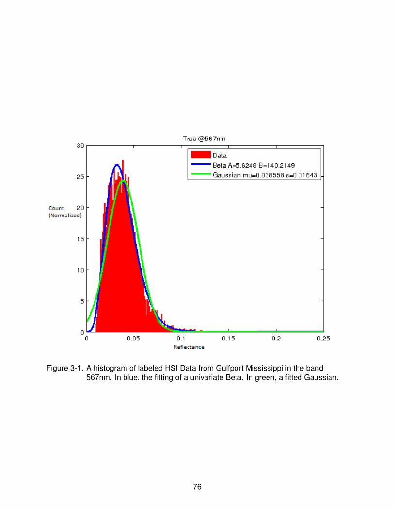
Figure 3-1. A histogram of labeled HSI Data from Gulfport Mississippi in the band567nm. In blue, the fitting of a univariate Beta. In green, a fitted Gaussian.

76

Figure 3-2. Plot of the independence copula in 2 Dimensions.

77

Figure 3-3. Plot of the Gaussian Copula in 2 Dimensions. With Σ =(1 0.30.3 1

)

78

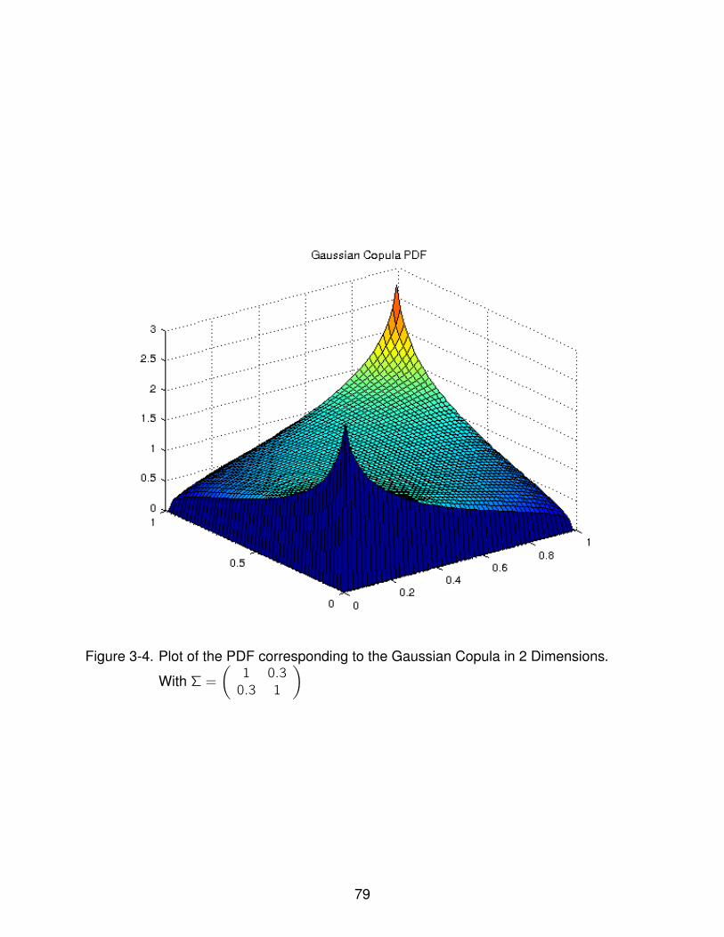
Figure 3-4. Plot of the PDF corresponding to the Gaussian Copula in 2 Dimensions.

With Σ =(1 0.30.3 1

)

79

CHAPTER 4RESULTS

After implementation of the unmixing approaches in the previous sections we ran

many different experiments in order to determine the efficacy of the BCM and CBCM,

the results of which appear in this chapter.

Broadly speaking we validate the models and unmixing algorithms used in two

ways, first using synthetic generated datasets and second using an AVIRIS dataset

collected over Gulfport Mississippi in 2010[66].

4.1 Synthetically Generated Data

Using real endmember distributions from hand-labeled remotely sensed data taken

over Gulfport Mississippi [66] we synthetically generated a dataset of 10,000 pixels.

Endmember distributions for Dirt (Fig. 4-2), Tree (Fig. 4-3), and Asphalt (Fig. 4-1) in

63 bands were selected and beta distributions were fit to them, generating a set of

parameters ~α, ~β.

These parameters ~α, ~β were then used, for every pixel, to sample an endmember

from each endmember distribution.

ek ∼ B(~αk , ~βk) for k ∈ {1, ...,M}. (4–1)

Then, combining this with a proportion vector sampled from a standard Dirichlet

distribution

pi ∼ Dir(1) (4–2)

Each pixel was generated as a dot product of endmembers and proportions

xi :=

M∑k=1

pi ,k ek (4–3)

80

and the dataset is simply given by X = {x1, ..., x10000}. Figure 4-4 shows a

visualization of 100 spectra in this dataset.

4.1.1 Unmixing Proportions

Unmixing solely the proportions was accomplished through BBCM (Section

3.4.4), with the mean and sample size estimation step omitted, in other words, a single

Metropolis-Hastings sampler.

The sampling itself was accomplished with 10000 iterations, with 1000 burn-in

iterations, and a sample was taken from every 10-th iteration to ensure independent

sampling : yielding 1000 total samples. The results of unmixing for this experiment were

measured through L1 error of the estimated proportions and the MAP of the resulting

sampled proportions, which was estimated by taking the mean of the samples. Fitting

a normal distribution and taking a MAP estimate at the mode proved to be statistically

insignificant in terms of error difference.

Results can be seen in Table 4-1, comparison with the NCM, LMM, and [75] on this

same dataset is also given. The implementation of NCM used had diagonal covariance

matrices and is described in more detail in Section 4.3.4, The parameters for these

distributions were set such that the first two moments of all endmember distributions

were the same in all models.

This result represents an error of, on average, 3.7% for proportions estimated

for the model. The likelihood of the MAP estimate was within 0.03 % of the likelihood

of the truth, indicating that the error in the model is solely due to the high variance of

the endmember distributions. Indeed the error is highest for Dirt and Asphalt, whose

distributions have similar shape (Figures 4-2,4-1).

The error for the uniform proposal distribution (Eqn. 3–35) is identical up to the

precision used, however convergence of the MCMC sampler to within 1% of the

maximum likelihood required 20% less iterations. Therefore this proposal distribution

was used for all future experiments with BBCM.

81

Comparing the results of BCM with the results of other state of the art unmixing

methods, it is clear that the BCM performs better at unmixing overall, performing 5−10%

better than the NCM. Though the NCM does surprisingly well on data which is not

normally distributed. Note that BBCM performs overwhelmingly better than the first

method developed to unmix the BCM in [75], also shown in the table, which was not

designed to work well with highly mixed data.

4.1.2 Endmember Distribution Estimation

Determining the endmember distributions with known proportions on the synthetic

dataset described above was accomplished through BBCM 3.4.4, with the proportion

estimation step substituted with the true proportions for every sample. This effectively

turns BBCM from a 3-stage Gibbs sampler into a 2-stage Gibbs sampler.

The sampling itself was accomplished with 1000 iterations of the global Gibbs

sampler and 100 burn in iterations, with a sample was taken from every 5-th iteration to

avoid dependency in sampling : yielding 200 total samples. Within each Metropolis-Hastings

step, for the mean a burn-in of 200 iterations was used per sample, and for the sample

size a burn-in of 100 iterations was used.

The results of unmixing for this experiment were measured through L1 error of

the estimated means and the true means of the three endmember distributions. Also,

relative L1 error was used between the estimated and true sample sizes to determine

the accuracy of the estimation. Results appear in Table 4-2.

BBCM was able to effectively estimate the endmember distributions, given the

known proportions, with virtually no error in estimating the mean, and an average

relative error of roughly 3% when estimating the sample size, again the likelihood of the

MAP estimate was within 0.1% of the truth likelihood, so this error is again due to the

variance of the distributions.

82

4.1.3 Full Unmixing

The two previous experiments serve as a baseline for the accuracy of the full

BBCM method. With this in mind, The full BBCM was tested on the synthetic dataset

introduced above. The sampling itself was accomplished with 1000 iterations of the

global Gibbs sampler and 100 burn in iterations, with a sample was taken from every

5-th iteration to avoid dependency in sampling : yielding 200 total samples. Within each

Metropolis-Hastings step, for the mean a burn-in of 200 iterations was used per sample,

and for the sample size a burn-in of 100 iterations was used, and for the proportions a

burn-in of 100 iterations was used per sample.

The results of unmixing for this experiment were measured through L1 error of the

estimated means and the true means of the three endmember distributions, relative L1

error between the estimated and true sample sizes, and absolute L1 error between the

estimated and true proportions for each endmember. Results appear in Table 4-3.

The true and estimated means appear in Figure 4-8 and the true and estimated

sample sizes in Figure 4-9. The algorithm derived in this research was able to fully

unmix the Beta Compositional Model with minimal error on this synthetic dataset.

Indeed, the error in the mean is less than 1% reflectance, and the error in proportion

is about 4%, not far from the baseline 3% from previous experiments with fixed

endmember distributions. Furthermore, the MAP estimate, that is to say the estimated

full set of parameters ~µ, ~SS,P, had a likelihood that was 0.5% greater than the likelihood

of the true parameters. This indicates strongly that the errors in this experiment are not

due to the algorithm, but due to the inherent variance of the endmember distributions.

4.2 Experiments with the Gulfport Dataset

Using an AVIRIS dataset collected over Gulfport Mississippi in 2010[66] with

co-registered ground measurements corresponding to endmember distributions, a

91 × 126 sub-image of the campus area was selected which is shown in Figure 4-10.

83

This area has a large area of tree cover, a large building with a very visible grey roof,

several paved roadways and a parking lot, and small localized areas with grass and dirt.

Two types of ground truth are available on this dataset, with varying degrees of

accuracy. First, a set of measurements were collected on the ground with a hand-held

device, for 32 different classes, ranging from 5 to 50 measurements per spectral group.

Second, a hand labeling of a superset of this dataset, shown in Figure 4-11, was done,

where regions of pure or nearly-pure pixels were identified within the scene using the

remotely sensed data, Google Earth, and photos taken at the dataset collection itself, for

guidance [66]. This ground truth is less accurate, but there is an abundance of it : a total

of 8 classes with over 1000 pixels per class.

In order to evaluate the effectiveness of BBCM at fully unmixing the endmember

distributions, we compare the ground collected truth to the distributions generated

by BBCM by firstly, labeling each endmember distribution by taking the mean and

identifying the category in which the closest ground-collected spectra (by L1 norm)

resides. Qualitative comparison can then be done by comparing each associated

proportion map with the hand-labeled truth.

For the second group of hand-labeled airborne truth, we evaluate the result by

comparing the labeled proportion maps with proportion maps (generated by labeling the

image by the maximum proportion of each distribution) estimated by BBCM.

We proceeded to unmix this area fully using BBCM with 5 endmembers, 3000

burn-in iterations and 6000 total iterations with a sample taken from every 5-th iteration,

yielding 600 samples. Resulting endmember distribution means with closest ground

spectra in Figure 4-12, with the distributions themselves in Figure 4-14, and proportion

maps labeled by matching closest ground spectra are shown in Figure 4-13. The

labelings themselves and associated error are given in Table 4-4.

84

4.2.1 Comparison with NCM

We also ran an NCM unmixing algorithm, as implemented by Eches et. al. [10]

with MATLAB code provided. Comparison with the BBCM is difficult, however, as there

is as of the moment of this writing, no full Bayesian unmixing algorithm for the NCM.

Ineed, Eches et al. do not estimate the endmember means for the NCM, and assume

covariance is diagonal and scalar and the same for each endmember distribution. We

use the means generated by BCM as fixed parameters to the NCM unmixing algorithm

[10].

We unmixed this same area of Gulfport fully with this method, using 3000 burn-in

iterations and 6000 total iterations with again a sample taken from every 5-th iteration,

yielding 600 samples. We compare this NCM unmixing method to BBCM in terms of

generated endmember distributions and proportion maps.

Concerning endmember distributions observe the generated tree distributions,

Figures 4-15, 4-16, and the corresponding ground truth in Figure 4-17, as well as

hand labeled truth in Figure 4-3. The BBCM is more accurately able to estimate the

shape of the true endmember distribution than the NCM, with an average band-wise KL

divergence of 3.51 from the truth (compared to 26.83 for the NCM). This is indicative

of BBCMs ability in general to provide a better estimate of the variance compared to

this implementation of the NCM. Indeed, a scalar covariance (as implemented in [10])

appears to be insufficient to describe most endmember distributions.

4.3 BCBCM Experiments

To empirically validate the CBCM model, experiments were performed on two

different types of datasets. First, a purely synthetic dataset, and finally a dataset

consisting of a mixture of real endmember distributions. Quantitative comparisons with

NCM and LMM models are available for each experiment and analyzed in detail. Before

this is done, the method in section 3.5.2 is described in detail and empirically verified, as

it is vital to the efficacy of this model.

85

4.3.1 Covariance Mapping

An interpolation based approximation to the mapping given in the preceding

chapter, given below, is constructed for the Gaussian Copula as follows.

FS(σ) := Covσ(b1,b2) ∗1√V1V2

(4–4)

S := {Params(b1),Params(b2)} (4–5)

First we select a set of parameters for each of the marginals, 50 uniformly spaced

means µ1,µ2 ∈ [0, 1], and 50 non-uniformly placed sample sizes. ss1, ss2 ∈ (1,∞).

Recall that the beta distribution can be parametrized in this way, in terms of mean and

sample size.

Note that it can be shown that ss1, ss2 →∞, F1,2(σ)→ σ.

For each distinct set of marginal parameters S = {ss1, ss2,µ1,µ2}, of which there

were 6.2 million, we calculated the sample covariance for two cases, σ = 1 and σ = 0.5

using 200,000 samples from a bivariate Gaussian copula with this σ. Note that, by

independence, FS(0) = 0.

Calculating FS(1),FS(0.5) for each S , the mappings ˆF (1) and F (0.5) are estimated

by two 4-D linear interpolation over all possible marginal parameters S (with the aid of

MATLAB software).

Then F is estimated in its entirety by fitting a quadratic polynomial in σ.

FS(σ) = aσ2 + bσ (4–6)

a := −4F (0.5) + 2F (1) (4–7)

b := 4F (0.5)− 1F (1) (4–8)

Where a, b are calculated from ˆF (1), F (0.5) by solving a linear system. A linear and

piecewise linear fit was also explored, but found to perform worse in terms of accuracy,

86

although slightly faster in terms of unmixing speed. A depiction of this mapping, as well

as various different fittings for a given S is shown in Figure 4-6. This quadratic/linear

approximation of F was used for all subsequent experiments.

4.3.2 Synthetic Dataset

Using beta endmember distributions fitted to hand-labeled remotely sensed data

taken over Gulfport Mississippi [66] we synthetically generated a dataset of 10,000

pixels. Endmember distributions for Dirt (Fig. 4-2), Tree (Fig. 4-3), and Asphalt (Fig. 4-1)

in 63 bands were selected and beta distributions were fit to them, generating a set of

parameters ~α, ~β,Cm, similarly as in the dataset described in Section 4.1.

Some extra detail is necessary here, as while it is simple to fit univariate distributions

to each band, it is more involved to fit a multivariate distribution with given marginals and

copula. The way we approached this problem is by first fitting marginal distributions

to the first and second moments of the data. Then, the mapping determined in the

preceding section was used to determine the parameters of the Gaussian copula Cm for

each pair of marginals.

Once generated, these parameters ~α, ~β,Ck were then used, for every pixel, to

sample an endmember from each endmember distribution.

ek ∼ B(~αk , ~βk ,Ck) for k ∈ {1, ...,M}. (4–9)

Then, as in the independence case, combining this with a proportion vector sampled

from a standard Dirichlet distribution

pi ∼ Dir(1) (4–10)

Each pixel was generated as a dot product of endmembers and proportions

87

xi :=

M∑k=1

pi ,k ek (4–11)

and the dataset is simply given by X = {x1, ..., x10000}. Figure 4-5 shows a

visualization of 100 spectra in this dataset, note the difference with Figure 4-4.

4.3.3 Mixture of True Distributions

A hybrid dataset consisting of real data from endmember distributions collected

in Gulfport Mississippi [66] was also created. The idea behind such a dataset was to

assess the performance of the model (compared to other state of the art models), on

data which mixes real endmember distributions, but still has an accurate form of ground

truth.

Indeed, this dataset is similar to the one described in the preceding section,

however, crucially, when sampling an endmember from each endmember distribution,

we sampled from the true histogram of all endmembers in the distribution, of which there

were 5000− 10000 depending on the distribution.

ek ∼ Histk for k ∈ {1, ...,M}. (4–12)

To get a grasp on the goodness of fit between Histk and the multivariate beta, the

KL divergence between the histograms for the marginals of these three endmember

distributions was calculated and can be seen in figure 4-7.

The mixture proportions were generated synthetically, using a standard Dirichlet as

in the previous dataset,

pi ∼ Dir(1) (4–13)

88

Yielding an accurate form of ground truth. The motivation for the creation of this

hybrid dataset was to compare the NCM and BCM on a mixture of true endmember

distributions that were collected from real data. Comparison is possible, in this case,

because the true proportions are known. We refer to this dataset as the ”True Mixture”

dataset, denoted XT .

4.3.4 Comparison with NCM, LMM, and BCM

Both datasets were unmixed with five different state of the art methods. First,

the standard linear mixing model, Second, a method of unmixing with the Normal

Compositional Model with full and diagonal covariance matrices. No such method

exists in the literature, but simple implementation changes to BCBCM were made to

accommodate such a method, (simply by replacing the covariance mapping with the

identity, and swapping the marginals to normals). Third, the proportion unmixing part

of BBCM method in the previous chapter was also run, for comparison. And finally,

BCBCM was also run.

For the NCM, BCM, and BCBCM methods, a Metropolis Hastings algorithm was

used described earlier in the preceding sections. A uniform prior and a uniform proposal

distribution was used for all methods.

For consistency all methods were given the same number of iterations 10000 with

samples taken from every 30th iteration. The MAP estimate, PE , of the proportions for

each method was taken as the mean of the histogram of samples.

Efficacy of each method was compared via the following L1-based measure for

endmember distribution k , where PT denotes the true proportions, and PE denotes the

estimated proportion.

ERRk :=1

N

N∑i=1

|PEi ,k − PTi ,k | (4–14)

89

These results were also combined to determine a global error measure for the

whole dataset.

ERR :=1

NM

M∑k=1

N∑i=1

|PEi ,k − PTi ,k | (4–15)

In other words, the average of the errors for each endmember distribution. Recall

that N = 10000 and M = 3 for both datasets in question. Results for the first synthetic

dataset appear in Table 4-5.

Predictably, the CBCM model is superior and outperforms all other methods. If data

is really distributed as multivariate beta distributions, BCBCM outperforms state of the

art by as much as 10%.

Note the high error in the LMM as well, this is strong evidence that the fixed-spectra

endmember assumption is not valid if the data is indeed distributed as a convex sum of

random variables.

A more interesting result from unmixing of the true mixture dataset appears in Table

4-6. Note again the high error in the LMM, even higher than in the previous dataset.

However, despite the fact that, as can be seen in Figure 4-7, the marginals are a better

fit, the CBCM model does no better than the NCM. There are two plausible explanations

for this.

In the NCM, a Gaussian copula is implicit, as the marginals are Gaussian, no

approximation is necessary. However in the CBCM we approximate this dependence

with a Gaussian Copula, which we in turn also approximate through a mapping. The

mapping was found to have an absolute maximum error of 0.02 for any σ, and an

average estimation error of 0.002 for a random sampling of 1000 pixels. Yet, because

the likelihood is dominated by the dependence term, the marginals play less of a role,

and our approximation error is magnified, no such approximation error is inherent in the

NCM.

90

It is tempting to attribute this error to approximation, yet, puzzlingly, the error

observed on the second dataset does not occur on the truly synthetic dataset generated

from multivariate beta distributions. Indeed the result on both of these datasets is strong

evidence that while marginally beta distributions fit hyperspectral data better than normal

distributions (Figure 4-7), multivariate beta distributions do not fit hyperspectral data any

better than multivariate normal distributions, if the copula used is Gaussian.

We conclude that CBCM accurately fits mixtures of real endmember distributions

in hyperspectral data, effectively just as well as the NCM. However the increased

complexity of the model and increased time complexity over NCM is enough to favor use

of the NCM rather than the CBCM for unmixing real hyperspectral data (Table 4-6), if

endmember distribution dependency information is available. If such information is not

available, then experiments in the preceding section indicate ordinary BCM is superior to

NCM for unmixing.

300 400 500 600 700 800 900 1000 11000

0.1

0.2

0.3

0.4

0.5

0.6

0.7

0.8

0.9

1Asphalt

Wavelength

Ref

lect

ance

Figure 4-1. A distribution of spectra for pixels that contain purely or near purely asphalt,taken from Gulfport, Mississippi.

91

300 400 500 600 700 800 900 1000 11000

0.1

0.2

0.3

0.4

0.5

0.6

0.7

0.8

0.9

1Dirt

Wavelength

Ref

lect

ance

Figure 4-2. A distribution of spectra for pixels that contain purely or near purely dirt,taken from Gulfport, Mississippi.

300 400 500 600 700 800 900 1000 11000

0.1

0.2

0.3

0.4

0.5

0.6

0.7

0.8

0.9

1Tree

Wavelength

Ref

lect

ance

Figure 4-3. A distribution of spectra for pixels that contain purely or near purely tree,taken from Gulfport, Mississippi.

92

300 400 500 600 700 800 900 10000

0.1

0.2

0.3

0.4

0.5

0.6

0.7

0.8

0.9

1Synthetic Dataset

Wavelength

Ref

lect

ance

Figure 4-4. 100 Spectra taken from the Synthetic Dataset

400 500 600 700 800 900 10000

0.05

0.1

0.15

0.2

0.25

0.3

0.35

0.4

0.45

0.5

Wavelength (nm)

Ref

lect

ance

Synthetic Dataset

Figure 4-5. 100 Spectra taken from a Copula-Based Synthetic Dataset

93

0 0.1 0.2 0.3 0.4 0.5 0.6 0.7 0.8 0.9 1−0.018

−0.016

−0.014

−0.012

−0.01

−0.008

−0.006

−0.004

−0.002

0

Sigma

F(S

igm

a) −

Sig

ma

Copula to Covariance Mapping for Two Beta Distributions

SamplesPolynomial FitLinear Fit

Figure 4-6. Approximating a mapping between Covariance and Copula Correlation.

1,000,000 Samples were used to estimate F(Sigma) at each point.

Table 4-1. Proportion Unmixing Errors for BCM with a Mean-based ProposalDistribution. Comparison with NCM, LMM, and the BCM unmixing method in[75] (Old BCM) on the same data.

Model Tree Asphalt Dirt AverageBCM 0.024 0.042 0.044 0.037NCM 0.026 0.045 0.046 0.039LMM 0.031 0.068 0.065 0.055

Old BCM 0.075 0.089 0.090 0.085

Table 4-2. L1 Error in mean Estimation (Absolute) and L1 Error in Sample size (Relative)Tree Dirt Asphalt

Error in Mean 0.0008 0.0006 0.0009Error in Sample Size 0.0429 0.0317 0.0237

94

Table 4-3. A table showing error values between the MAP estimate and the ground truth.Tree Dirt Asphalt Average

Error in Mean 0.0032 0.0039 0.0044 0.0038Error in Sample Size 0.0756 0.0305 0.0926 0.0662

Error in Proportion 0.0280 0.0471 0.0499 0.0417

Table 4-4. A table showing labelings for the mean and associated distance to truth(average L1 error in each band).

BCM Label L1 DistanceOak Tree (Friendship Oak) 0.0253

Shadow 0.0270Dried Leaves 0.0206

Asphalt 0.0553Sidewalk 0.0311

Table 4-5. A table showing error values between the MAP estimate and the ground truthfor different models on a synthetic dataset. NCM-d is NCM with a diagonalcovariance.

Model Tree Dirt Asphalt Average Seconds / SampleLMM 0.1151 0.2496 0.2138 0.1928 0.00

NCM-d 0.1163 0.1830 0.1329 0.1441 1.78BCM 0.1158 0.1782 0.1300 0.1413 6.51NCM 0.0339 0.0616 0.0658 0.0538 81.91

CBCM 0.0330 0.0517 0.0563 0.0470 222.30

Table 4-6. A table showing error values between the MAP estimate and the ground truthfor different models on a dataset with mixtures of true endmemberdistributions.Tree Dirt Asphalt Average Seconds / Sample

LMM 0.1170 0.2532 0.2163 0.1955 0.00NCM-d 0.1168 0.1819 0.1282 0.1423 1.43

BCM 0.1169 0.1769 0.1257 0.1398 6.79NCM 0.0301 0.0601 0.0633 0.0511 80.97

CBCM 0.0331 0.0594 0.0650 0.0525 220.11

95

A Tree

B Dirt

C Asphalt

Figure 4-7. In Blue is the KL Divergence of the Beta Distribution Fit for each Band. InGreen the same information for the Gaussian. The Beta is a clear better fitfor Tree and Asphalt.

96

400 500 600 700 800 900 10000

0.05

0.1

0.15

0.2

0.25

0.3

0.35

0.4

0.45

Wavelength

Mea

n

Mean of Endmember Distributions (Estimated vs True)

ED Tree estimatedED Asphalt estimatedED Dirt estimatedED Tree trueED Asphalt trueED Dirt true

Figure 4-8. Estimated and True Mean values of the Endmember Distributions withSynthetic Data

400 500 600 700 800 900 10000

100

200

300

400

500

600

700

800

900

Wavelength

Sam

ple

Siz

e

Sample Size of Endmember Distributions (Estimated vs True)

Tree estimatedAsphalt estimatedDirt estimatedTree trueAsphalt trueDirt true

Figure 4-9. Estimated and True Sample Size of the Endmember Distributions withSynthetic Data

97

Gulfport Mississippi

20 40 60 80 100 120

10

20

30

40

50

60

70

80

90

Figure 4-10. A part of the campus area in the Gulfport Mississippi dataset.

20 40 60 80 100 120

180

200

220

240

260

280

Figure 4-11. A class partition used to evaluate the efficacy of resulting proportion maps.

98

500 600 700 800 900 10000

0.1

0.2

0.3

0.4

0.5

0.6

0.7

0.8

Wavelength

Endmembers and Closest Ground Spectra L2 Norm, AVG ERR=0.10667

FriendshipOak : ERR=0.070248Shadow : ERR=0.052288DriedLeaves : ERR=0.057737AsphaltBeachParkingLot : ERR=0.2721SidewalkInShade : ERR=0.080968

Figure 4-12. Means of endmember distributions computed by BBCM.

99

FriendshipOak

20 40 60 80 100 120

20

40

60

80

Shadow

20 40 60 80 100 120

20

40

60

80

DriedLeaves

20 40 60 80 100 120

20

40

60

80

AsphaltBeachParkingLot

20 40 60 80 100 120

20

40

60

80

SidewalkInShade

20 40 60 80 100 120

20

40

60

80

Figure 4-13. Proportions computed by BBCM.

100

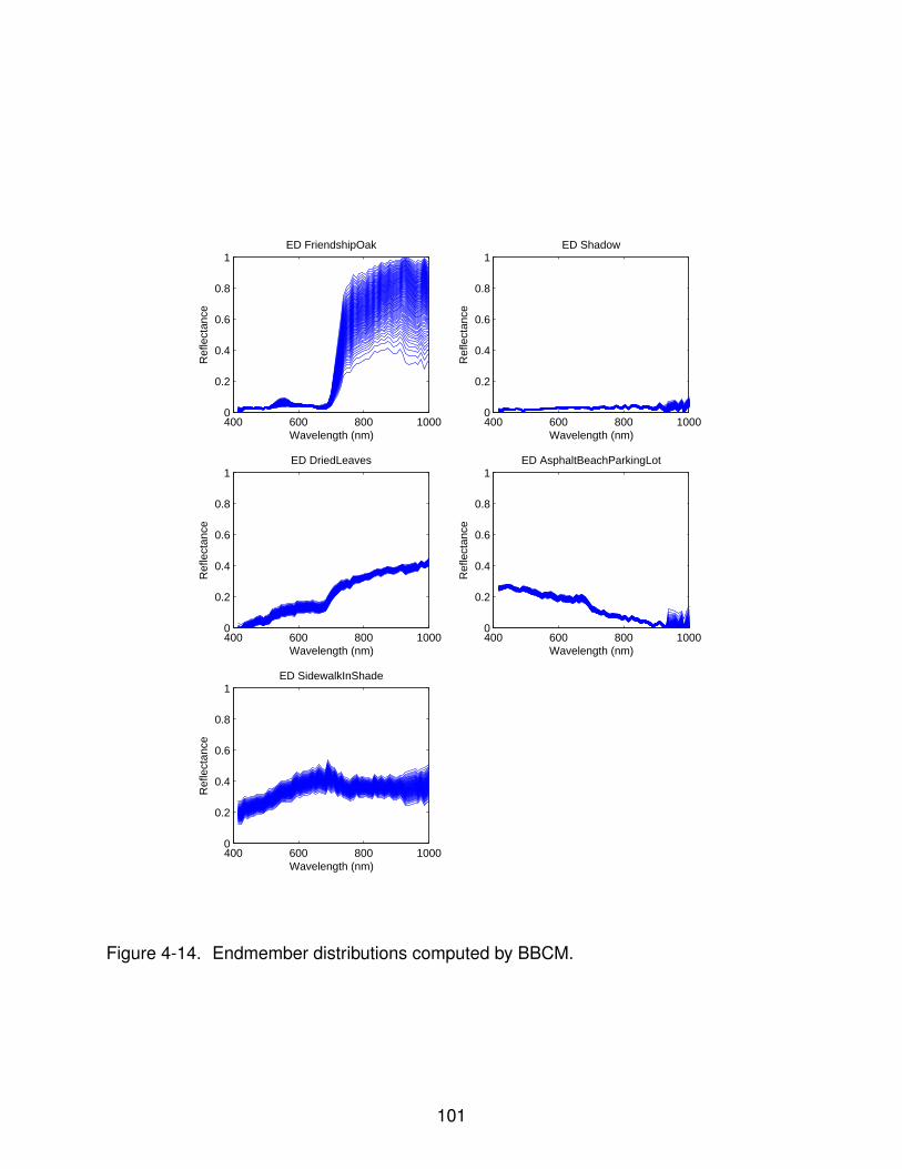
400 600 800 10000

0.2

0.4

0.6

0.8

1

Wavelength (nm)

ED FriendshipOak

Ref

lect

ance

400 600 800 10000

0.2

0.4

0.6

0.8

1

Wavelength (nm)

ED Shadow

Ref

lect

ance

400 600 800 10000

0.2

0.4

0.6

0.8

1

Wavelength (nm)

ED DriedLeaves

Ref

lect

ance

400 600 800 10000

0.2

0.4

0.6

0.8

1

Wavelength (nm)

ED AsphaltBeachParkingLotR

efle

ctan

ce

400 600 800 10000

0.2

0.4

0.6

0.8

1

Wavelength (nm)

ED SidewalkInShade

Ref

lect

ance

Figure 4-14. Endmember distributions computed by BBCM.

101

400 500 600 700 800 900 1000 11000

0.1

0.2

0.3

0.4

0.5

0.6

0.7

0.8

0.9

1ED FriendshipOak : Uniform Sampling

Figure 4-15. The tree distribution as estimated by BBCM.

400 500 600 700 800 900 10000

0.1

0.2

0.3

0.4

0.5

0.6

0.7

0.8

0.9

1

Wavelength (nm)

ED FriendshipOak

Ref

lect

ance

Figure 4-16. The tree distribution as estimated with NCM.

102

0 100 200 300 400 500 600 700 8000

0.1

0.2

0.3

0.4

0.5

0.6

0.7

0.8

0.9

1FriendshipOak

Figure 4-17. A Tree Distribution from the Ground-collected Truth in the Gulfport Data.

103

CHAPTER 5CONCLUSION

The introduced Beta Compositional (BCM, CBCM) family of models addresses

major issues present in the current state of the art approach to endmember distribution

estimation, the Normal Compositional Model (NCM). In particular, the CBCM’s support

is physically valid in the domain of reflectance, band-wise dependency of endmember

can be represented, and the shape of the beta distribution provides, marginally, a better

reflection of the observed asymmetry than the Gaussian.

Furthermore, two novel, Bayesian, endmember distribution estimation algorithms

are derived, implemented, and tested for this family of models. These algorithms are

based heavily on Markov-Chain Monte Carlo methods, but this approach parallels, in

some sense, existing algorithms for unmixing the NCM.

The development of one of these algorithms, BCBCM, led to a novel theoretical

result relating copula to covariance, and as a result a general method to modeling sums

of copula-based random variables was discovered, with potential applications even

outside the field of hyperspectral. On the other hand, the development of BBCM showed

that a fully Bayesian unmixing approach for a distribution based hyperspectral model

is feasible. Such an approach proved effective at estimating endmember variability,

more-so than existing NCM unmixing methods.

We conclude that the Beta Compositional Family of models plus derived Bayesian

unmixing methods are not only an improvement upon state of the art, but also a step

forward in the field of hyperspectal, paving the way for other distribution-based models of

endmember spectral variability that follow a similar approach.

104

REFERENCES

[1] J. Bioucas-Dias, A. Plaza, N. Dobigeon, M. Parente, Q. Du, P. Gader, andJ. Chanussot, “Hyperspectral unmixing overview: Geometrical, statistical, andsparse regression-based approaches,” Selected Topics in Applied Earth Observa-tions and Remote Sensing, IEEE Journal of, vol. 5, no. 2, pp. 354–379, 2012.

[2] N. Keshava and J. Mustard, “Spectral unmixing,” Signal Processing Magazine,IEEE, vol. 19, no. 1, pp. 44–57, 2002.

[3] R. Close, “Endmember and proportion estimation using physics-based macroscopicand microscopic mixture models,” Ph.D. dissertation, UNIVERSITY OF FLORIDA,2012.

[4] D. Stein, “Application of the normal compositional model to the analysis ofhyperspectral imagery,” in Advances in Techniques for Analysis of RemotelySensed Data, 2003 IEEE Workshop on. IEEE, 2003, pp. 44–51.

[5] B. Somers, G. P. Asner, L. Tits, and P. Coppin, “Endmember variability in spectralmixture analysis: A review,” Remote Sensing of Environment, vol. 115, no. 7, pp.1603–1616, 2011.

[6] A. Zare and P. Gader, “An investigation of likelihoods and priors for bayesianendmember estimation,” in AIP Conference Proceedings, vol. 1305, 2011, p. 311.

[7] T. Schmidt, “Coping with copulas,” Chapter forthcoming in Risk Books: Copulas,from theory to applications in finance, 2006.

[8] C. Bishop et al., Pattern recognition and machine learning. springer New York,2006, vol. 4, no. 4.

[9] F. Schmidt, A. Schmidt, E. Treguier, M. Guiheneuf, S. Moussaoui, and N. Dobigeon,“Implementation strategies for hyperspectral unmixing using bayesian sourceseparation,” Geoscience and Remote Sensing, IEEE Transactions on, vol. 48,no. 11, pp. 4003–4013, 2010.

[10] O. Eches, N. Dobigeon, C. Mailhes, and J. Tourneret, “Bayesian estimation oflinear mixtures using the normal compositional model. application to hyperspectralimagery,” Image Processing, IEEE Transactions on, vol. 19, no. 6, pp. 1403–1413,2010.

[11] M. Berman, H. Kiiveri, R. Lagerstrom, A. Ernst, R. Dunne, and J. Huntington,“Ice: A statistical approach to identifying endmembers in hyperspectral images,”Geoscience and Remote Sensing, IEEE Transactions on, vol. 42, no. 10, pp.2085–2095, 2004.

[12] J. Boardman, F. Kruse, and R. Green, “Mapping target signatures via partialunmixing of aviris data,” 1995.

105

[13] J. Boardman et al., “Automating spectral unmixing of aviris data using convexgeometry concepts,” in Summaries 4th Annu. JPL Airborne Geoscience Workshop,vol. 1. JPL Publication 93–26, 1993, pp. 11–14.

[14] A. Green, M. Berman, P. Switzer, and M. Craig, “A transformation for orderingmultispectral data in terms of image quality with implications for noise removal,”Geoscience and Remote Sensing, IEEE Transactions on, vol. 26, no. 1, pp. 65–74,1988.

[15] M. Winter, “N-findr: an algorithm for fast autonomous spectral end-memberdetermination in hyperspectral data,” in SPIE’s International Symposium on OpticalScience, Engineering, and Instrumentation. International Society for Optics andPhotonics, 1999, pp. 266–275.

[16] J. Lee, A. Woodyatt, and M. Berman, “Enhancement of high spectral resolutionremote-sensing data by a noise-adjusted principal components transform,” Geo-science and Remote Sensing, IEEE Transactions on, vol. 28, no. 3, pp. 295–304,1990.

[17] J. Nascimento and J. Dias, “Vertex component analysis: A fast algorithm to unmixhyperspectral data,” Geoscience and Remote Sensing, IEEE Transactions on,vol. 43, no. 4, pp. 898–910, 2005.

[18] R. Neville, K. Staenz, T. Szeredi, J. Lefebvre, and P. Hauff, “Automatic endmemberextraction from hyperspectral data for mineral exploration,” in Proc. 21st CanadianSymp. Remote Sens, 1999, pp. 21–24.

[19] J. Gruninger, A. Ratkowski, and M. Hoke, “The sequential maximum angle convexcone(smacc) endmember model,” in Proceedings of SPIE, vol. 5425, 2004, pp.1–14.

[20] C. Chang, C. Wu, W. Liu, and Y. Ouyang, “A new growing method for simplex-basedendmember extraction algorithm,” Geoscience and Remote Sensing, IEEE Transac-tions on, vol. 44, no. 10, pp. 2804–2819, 2006.

[21] T. Chan, W. Ma, A. Ambikapathi, and C. Chi, “A simplex volume maximizationframework for hyperspectral endmember extraction,” Geoscience and RemoteSensing, IEEE Transactions on, vol. 49, no. 11, pp. 4177–4193, 2011.

[22] C. Wu, S. Chu, and C. Chang, “Sequential n-findr algorithms,” in Optical Engi-neering+ Applications. International Society for Optics and Photonics, 2008, pp.70 860C–70 860C.

[23] L. Miao and H. Qi, “Endmember extraction from highly mixed data using minimumvolume constrained nonnegative matrix factorization,” Geoscience and RemoteSensing, IEEE Transactions on, vol. 45, no. 3, pp. 765–777, 2007.

106

[24] D. Lee, H. Seung et al., “Learning the parts of objects by non-negative matrixfactorization,” Nature, vol. 401, no. 6755, pp. 788–791, 1999.

[25] M. Arngren, M. Schmidt, and J. Larsen, “Bayesian nonnegative matrix factorizationwith volume prior for unmixing of hyperspectral images,” in Machine Learning forSignal Processing, 2009. MLSP 2009. IEEE International Workshop on. IEEE,2009, pp. 1–6.

[26] A. Zare and P. Gader, “Sparsity promoting iterated constrained endmemberdetection in hyperspectral imagery,” Geoscience and Remote Sensing Letters,IEEE, vol. 4, no. 3, pp. 446–450, 2007.

[27] J. Bioucas-Dias, “A variable splitting augmented lagrangian approach to linearspectral unmixing,” in Hyperspectral Image and Signal Processing: Evolution inRemote Sensing, 2009. WHISPERS’09. First Workshop on. IEEE, 2009, pp. 1–4.

[28] J. Li and J. Bioucas-Dias, “Minimum volume simplex analysis: a fast algorithm tounmix hyperspectral data,” in Geoscience and Remote Sensing Symposium, 2008.IGARSS 2008. IEEE International, vol. 3. IEEE, 2008, pp. III–250.

[29] T. Chan, C. Chi, Y. Huang, and W. Ma, “A convex analysis-based minimum-volumeenclosing simplex algorithm for hyperspectral unmixing,” Signal Processing, IEEETransactions on, vol. 57, no. 11, pp. 4418–4432, 2009.

[30] G. Box and G. Tiao, “Bayesian inference in statistical analysis,” DTIC Document,Tech. Rep., 1973.

[31] A. Zare and P. Gader, “Pce: Piecewise convex endmember detection,” Geoscienceand Remote Sensing, IEEE Transactions on, vol. 48, no. 6, pp. 2620–2632, 2010.

[32] N. Dobigeon, S. Moussaoui, J. Tourneret, and C. Carteret, “Bayesian separationof spectral sources under non-negativity and full additivity constraints,” SignalProcessing, vol. 89, no. 12, pp. 2657–2669, 2009.

[33] S. Moussaoui, C. Carteret, D. Brie, and A. Mohammad-Djafari, “Bayesian analysisof spectral mixture data using markov chain monte carlo methods,” Chemometricsand intelligent laboratory systems, vol. 81, no. 2, pp. 137–148, 2006.

[34] A. Mohammad-Djafari, “A bayesian approach to source separation,” arXiv preprintmath-ph/0008025, 2000.

[35] O. Eches, N. Dobigeon, C. Mailhes, and J. Tourneret, “Unmixing hyperspectralimages using a normal compositional model and mcmc methods,” in StatisticalSignal Processing, 2009. SSP’09. IEEE/SP 15th Workshop on. IEEE, 2009, pp.646–649.

[36] C. Robert, G. Casella, and C. Robert, Monte Carlo statistical methods. SpringerNew York, 1999, vol. 2.

107

[37] Q. Shao and J. Ibrahim, Monte Carlo methods in Bayesian computation. SpringerSeries in Statistics, New York, 2000.

[38] S. Chib and E. Greenberg, “Understanding the metropolis-hastings algorithm,” TheAmerican Statistician, vol. 49, no. 4, pp. 327–335, 1995.

[39] G. Casella and E. George, “Explaining the gibbs sampler,” The American Statisti-cian, vol. 46, no. 3, pp. 167–174, 1992.

[40] W. Gilks, N. Best, and K. Tan, “Adaptive rejection metropolis sampling within gibbssampling,” Applied Statistics, pp. 455–472, 1995.

[41] J. Nascimento and J. Bioucas-Dias, “Hyperspectral unmixing algorithm viadependent component analysis,” in Geoscience and Remote Sensing Sympo-sium, 2007. IGARSS 2007. IEEE International. IEEE, 2007, pp. 4033–4036.

[42] P. Comon, “Independent component analysis, a new concept?” Signal processing,vol. 36, no. 3, pp. 287–314, 1994.

[43] J. Nascimento and J. Dias, “Does independent component analysis play a role inunmixing hyperspectral data?” Geoscience and Remote Sensing, IEEE Transac-tions on, vol. 43, no. 1, pp. 175–187, 2005.

[44] J. Nascimento and J. Bioucas-Dias, “Hyperspectral unmixing based on mixturesof dirichlet components,” Geoscience and Remote Sensing, IEEE Transactions on,vol. 50, no. 3, pp. 863–878, 2012.

[45] J. Bioucas-Dias and J. Nascimento, “Hyperspectral subspace identification,”Geoscience and Remote Sensing, IEEE Transactions on, vol. 46, no. 8, pp.2435–2445, 2008.

[46] J. Diebolt and G. Celeux, “Asymptotic properties of a stochastic em algorithm forestimating mixing proportions,” Stochastic Models, vol. 9, no. 4, pp. 599–613, 1993.

[47] K. Knuth, “Bayesian source separation and localization,” in SPIE’s InternationalSymposium on Optical Science, Engineering, and Instrumentation. InternationalSociety for Optics and Photonics, 1998, pp. 147–158.

[48] D. Rowe, Multivariate Bayesian statistics: models for source separation and signalunmixing. Chapman & Hall/CRC, 2002.

[49] N. Dobigeon, S. Moussaoui, M. Coulon, J. Tourneret, and A. Hero, “Joint bayesianendmember extraction and linear unmixing for hyperspectral imagery,” SignalProcessing, IEEE Transactions on, vol. 57, no. 11, pp. 4355–4368, 2009.

[50] S. Moussaoui, D. Brie, A. Mohammad-Djafari, and C. Carteret, “Separation ofnon-negative mixture of non-negative sources using a bayesian approach andmcmc sampling,” Signal Processing, IEEE Transactions on, vol. 54, no. 11, pp.4133–4145, 2006.

108

[51] S. Moussaoui, H. Hauksdottir, F. Schmidt, C. Jutten, J. Chanussot, D. Brie,S. Doute, and J. Benediktsson, “On the decomposition of mars hyperspectraldata by ica and bayesian positive source separation,” Neurocomputing, vol. 71,no. 10, pp. 2194–2208, 2008.

[52] N. Dobigeon and J. Tourneret, “Library-based linear unmixing for hyperspectralimagery via reversible jump mcmc sampling,” in Aerospace conference, 2009 IEEE.IEEE, 2009, pp. 1–6.

[53] N. Dobigeon, J. Tourneret, and C. Chang, “Semi-supervised linear spectralunmixing using a hierarchical bayesian model for hyperspectral imagery,” Sig-nal Processing, IEEE Transactions on, vol. 56, no. 7, pp. 2684–2695, 2008.

[54] P. Green, “Reversible jump markov chain monte carlo computation and bayesianmodel determination,” Biometrika, vol. 82, no. 4, pp. 711–732, 1995.

[55] O. Eches, N. Dobigeon, and J. Tourneret, “Estimating the number of endmembersin hyperspectral images using the normal compositional model and a hierarchicalbayesian algorithm,” Selected Topics in Signal Processing, IEEE Journal of, vol. 4,no. 3, pp. 582–591, 2010.

[56] A. Stocker and A. Schaum, “Application of stochastic mixing models tohyperspectral detection problems,” in AeroSense’97. International Society forOptics and Photonics, 1997, pp. 47–60.

[57] T. Ferguson, “A bayesian analysis of some nonparametric problems,” The annals ofstatistics, pp. 209–230, 1973.

[58] R. Neal, “Markov chain sampling methods for dirichlet process mixture models,”Journal of computational and graphical statistics, vol. 9, no. 2, pp. 249–265, 2000.

[59] S. Niu, V. Ingle, D. Manolakis, and T. Cooley, “On the modeling of hyperspectralimaging data with elliptically contoured distributions,” in Hyperspectral Imageand Signal Processing: Evolution in Remote Sensing (WHISPERS), 2010 2ndWorkshop on. IEEE, 2010, pp. 1–4.

[60] M. Eismann, Hyperspectral remote sensing, 2012.

[61] Q. Du and H. Yang, “Similarity-based unsupervised band selection for hyperspectralimage analysis,” Geoscience and Remote Sensing Letters, IEEE, vol. 5, no. 4, pp.564–568, 2008.

[62] R. N. Clark, USGS digital spectral library. US Geological Survey, 2000.

[63] I. Research Systems, ENVI user’s guide. Research Systems, 2003.

[64] G. Swayze, R. CLARK, F. Kruse, S. Sutley, and A. Gallagher, “Ground-truthingaviris mineral mapping at cuprite, nevada,” in JPL, Summaries of the Third AnnualJPL Airborne Geoscience Workshop., vol. 1, 1992.

109

[65] E. Christophe, D. Leger, and C. Mailhes, “Quality criteria benchmark forhyperspectral imagery,” Geoscience and Remote Sensing, IEEE Transactionson, vol. 43, no. 9, pp. 2103–2114, 2005.

[66] P. Gader, R. Close, and A. Zare, “AVIRIS Data Collection over Gulfport,Mississippi,” personal communication, 2010.

[67] C. Andrieu, N. De Freitas, A. Doucet, and M. I. Jordan, “An introduction to mcmc formachine learning,” Machine learning, vol. 50, no. 1-2, pp. 5–43, 2003.

[68] C. P. Robert and G. Casella, Monte Carlo statistical methods. Citeseer, 2004, vol.319.

[69] S. Brooks, A. Gelman, G. Jones, and X.-L. Meng, Handbook of Markov ChainMonte Carlo. Taylor & Francis US, 2011.

[70] D. F. de Souza and F. A. da Silva Moura, “Multivariate beta regression.”

[71] M. S. Smith, “Bayesian approaches to copula modelling,” 2011.

[72] A. J. McNeil and J. Neslehova, “Multivariate archimedean copulas, d-monotonefunctions and l1-norm symmetric distributions,” The Annals of Statistics, pp.3059–3097, 2009.

[73] B. Johannesson and N. Giri, “On approximations involving the beta distribution,”Communications in Statistics-Simulation and Computation, vol. 24, no. 2, pp.489–503, 1995.

[74] A. K. Gupta and S. Nadarajah, “Handbook of beta distribution and its applications,”pp. 80–89, 2004.

[75] A. Zare, P. Gader, D. Dranishnikov, and T. Glenn, “Spectral unmixing using the betacompositional model,” in Hyperspectral Image and Signal Processing: Evolution inRemote Sensing, 2013. WHISPERS’13., 2013.

[76] D. Kugiumtzis and E. Bora-Senta, “Normal correlation coefficient of non-normalvariables using piece-wise linear approximation,” Computational Statistics, vol. 25,no. 4, pp. 645–662, 2010.

[77] M. C. Cario and B. L. Nelson, “Autoregressive to anything: Time-series inputprocesses for simulation,” Operations Research Letters, vol. 19, no. 2, pp. 51–58,1996.

[78] W. Hoeffding, “Masstabinvariante korrelationtheorie,” Schriften Math. Inst. Univ.Berlin, pp. 181–233, 1940.

[79] C. Cuadras, “On the covariance between functions,” Journal of Multivariate Analy-sis, vol. 81, no. 1, pp. 19–27, 2002.

[80] C. Meyer, “The bivariate normal copula,” arXiv preprint arXiv:0912.2816, 2009.

110

[81] H. Joe, “Parametric families of multivariate distributions with given margins,” Journalof multivariate analysis, vol. 46, no. 2, pp. 262–282, 1993.

[82] P. Embrechts, F. Lindskog, and A. McNeil, “Modelling dependence with copulas andapplications to risk management,” Handbook of heavy tailed distributions in finance,vol. 8, no. 1, pp. 329–384, 2003.

111

BIOGRAPHICAL SKETCH

Dmitri Dranishnikov received his Bachelor of Science degree in mathematics

from the University of Florida in 2008. He continued his studies at the University

of Florida and acquired a Master of Science in computer engineering in 2013. His

research interests include machine learning, Markov Chain Monte Carlo methods, and

Hyperspectral Image analysis.

112