Apache Spark MLlibMachine Learning Library for a parallel computing framework

Review by Renat Bekbolatov (June 4, 2015)

Spark MLlib is an open-source machine learning li-brary that works on top of Spark. It is included inthe standard Spark distribution and provides datastructures and distributed implementations of manymachine learning algorithms. This project is in activedevelopment, has a growing number of contributorsand many adopters in the industry.

This review will attempt to look at Spark MLlib fromthe perspective of parallelization and scalability. Inpreparation of this report, MLlib public documenta-tion, library guide and codebase (development snap-shot version of 1.4) was referenced[1]. While MLlibalso offers Python and Java API, we will focus onlyon Scala API.

There will be some technical terms that are outsidethe scope of this report, and we will not look at themin details. Instead we will explain just enough toshow how a specific MLlib component is implementedand, wherever possible, provide references for furtherindependent study if needed.

1 Execution Model

Iterations

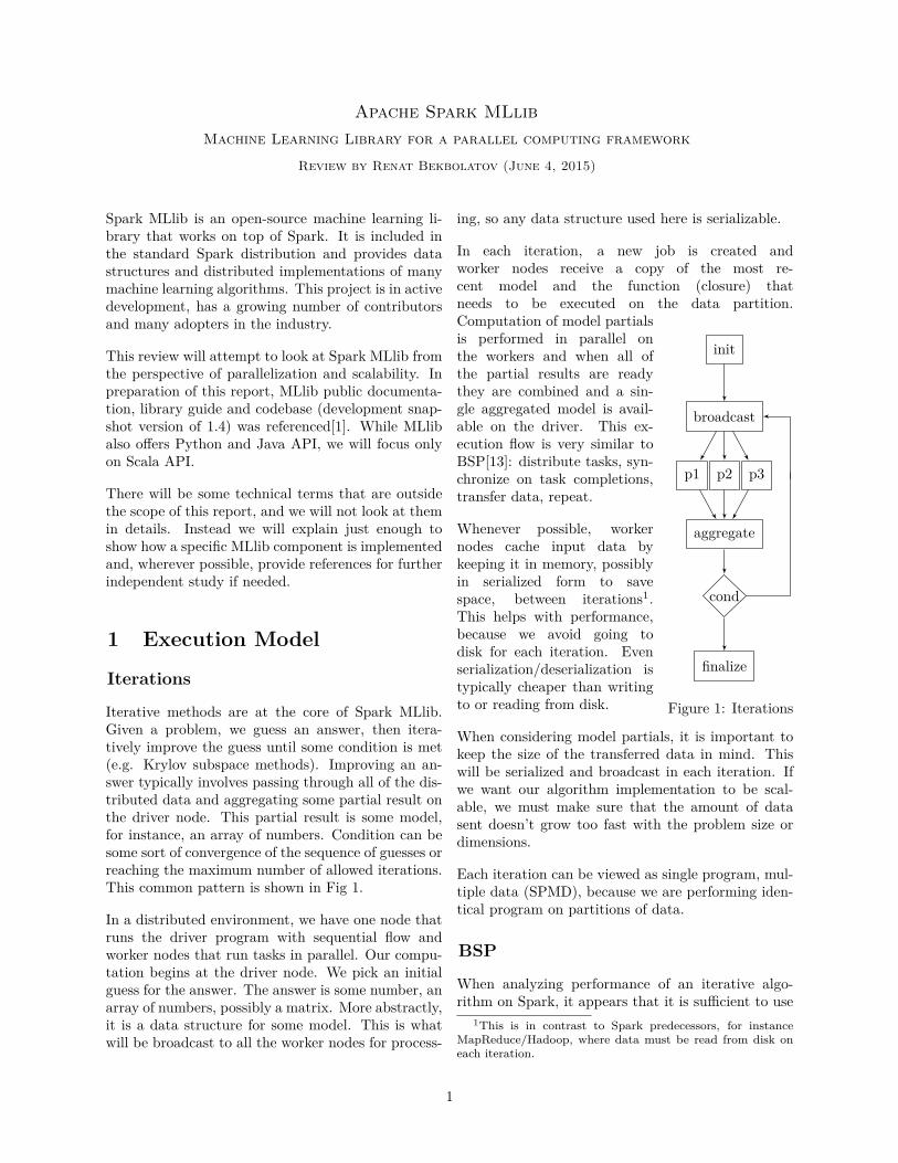
Iterative methods are at the core of Spark MLlib.Given a problem, we guess an answer, then itera-tively improve the guess until some condition is met(e.g. Krylov subspace methods). Improving an an-swer typically involves passing through all of the dis-tributed data and aggregating some partial result onthe driver node. This partial result is some model,for instance, an array of numbers. Condition can besome sort of convergence of the sequence of guesses orreaching the maximum number of allowed iterations.This common pattern is shown in Fig 1.

In a distributed environment, we have one node thatruns the driver program with sequential flow andworker nodes that run tasks in parallel. Our compu-tation begins at the driver node. We pick an initialguess for the answer. The answer is some number, anarray of numbers, possibly a matrix. More abstractly,it is a data structure for some model. This is whatwill be broadcast to all the worker nodes for process-

ing, so any data structure used here is serializable.

In each iteration, a new job is created andworker nodes receive a copy of the most re-cent model and the function (closure) thatneeds to be executed on the data partition.

init

broadcast

p1 p2 p3

aggregate

cond

finalize

Figure 1: Iterations

Computation of model partialsis performed in parallel onthe workers and when all ofthe partial results are readythey are combined and a sin-gle aggregated model is avail-able on the driver. This ex-ecution flow is very similar toBSP[13]: distribute tasks, syn-chronize on task completions,transfer data, repeat.

Whenever possible, workernodes cache input data bykeeping it in memory, possiblyin serialized form to savespace, between iterations1.This helps with performance,because we avoid going todisk for each iteration. Evenserialization/deserialization istypically cheaper than writingto or reading from disk.

When considering model partials, it is important tokeep the size of the transferred data in mind. Thiswill be serialized and broadcast in each iteration. Ifwe want our algorithm implementation to be scal-able, we must make sure that the amount of datasent doesn’t grow too fast with the problem size ordimensions.

Each iteration can be viewed as single program, mul-tiple data (SPMD), because we are performing iden-tical program on partitions of data.

BSP

When analyzing performance of an iterative algo-rithm on Spark, it appears that it is sufficient to use

1This is in contrast to Spark predecessors, for instanceMapReduce/Hadoop, where data must be read from disk oneach iteration.

1

BSP[13] model. Individual pair-wise remote memoryaccesses are below the abstraction layer and modelssuch as CTA and LogP do not provide additional ben-efit when operating with Spark abstractions[12, 14].

At the beginning of each iteration we broadcast tasksand wait for all the partitions to compute their par-tial results before combining them. This is sim-ilar to super-steps with barrier synchronization inBSP. Communication between processors is typicallydriver-to-all, and all-to-driver patterns1.

The most important factors of algorithm analysis onSpark are data partition schemes and individual par-tition sizes, partial model sizes and communicationlatency.

2 Infrastructure

Core Linear Algebra

Spark MLlib uses Breeze[2] and jblas[3] for basic lin-ear algebra. Both of these libraries are enriched wrap-pers around netlib[4], which make it possible to usenetlib packages through Scala or Java. Breeze is anumerical processing library that loads native netliblibraries if it they are available and gracefully fallsback to use their JVM versions. JVM versions areprovided by F2J library. Library jblas also uses netlibBLAS and LAPACK under the hood.

Using netlib for numeric computations not only helpsus improve speed of execution, better use of processorcaches, it also helps us deal with issues of precisionand stability of calculations2.

Local Data Types

Core MLlib data types are tightly integrated withBreeze data types. The most important local datatype is a Vector - which is stored internally as anarray of doubles. Two implementations are available:DenseVector and SparseVector3.

An extension of Vector is a concept of a LabeledPoint- which is an array of features: Vector, along with

1Communication will be explained in section Infrastructure,where aggregation and shuffle procedures are explained.

2Talk by Sam Halliday on high-performance linearalgebra in Scala, where he describes how one can ac-cess functionality of netlib native routines on JVM:https://skillsmatter.com/skillscasts/5849-high-performance-linear-algebra-in-scala

3Internally, both of these provide quick conversions to andfrom Breeze equivalents

a label (class) assignment, represented by a double.This is a useful construct for problems of supervisedlearning.

A local matrix is also available in MLlib: Matrix -and as the case with Vector, it is stored as an arrayof doubles, has two implementations: DenseMatrixand SparseMatrix4.

RDD: Distributed Data

MLlib builds upon Spark RDD construct. To use ML-lib functions, one would transform original data intoan RDD of vectors. Newer Spark MLlib function-ality allows operations on a higher-level abstraction,borrowed from other popular data processing frame-works: DataFrame. In a later section (3.1, LibraryFunctions: Distributed Matrices) we will discuss dis-tributed matrices in detail.

RDD[T] can be seen as a distributed list contain-ing elements of type T. One can transform RDDs bytransforming contained values in some way, and forcematerialization of some results of such transforma-tions through actions. Let us briefly go through afew basic transformations and actions.

Let us recap a couple of basic RDD operations. Con-sider an RDD of integer numbers, A, stored in 3 par-titions:

A← [[0, 1, 2, 3], [4, 5, 6], [7, 8, 9]]

Here our first partition contains [0, 1, 2, 3], secondcontains [4, 5, 6], and the last partition has [7, 8, 9].Now, we can create another RDD, B, as follows:

B ← A.map{n⇒ n+ 1}

B is now [[1, 2, 3, 4], [5, 6, 7], [8, 9, 10]]. We could per-form a reduction operation, say calculate the sum ofall elements in B with an action operation reduce:

sum← B.reduce{(a, b)⇒ a+ b}

Calling reduce starts a computation that will toucheach element in each partition and combine resultsinto a single value that will be available on the drivernode.

Aggregations

Action reduce might be the simplest non-trivial ag-gregation operation. It requires that the type of the

4Again, internally, Breeze matrix conversions are also pro-vided

2

output of the reduction function is same as the typeof the values stored in RDD. In each partition, thisreduction function will be applied to values in thatpartition and the running partial result. Then eachof the partial results is sent to the driver node andthe same reduction application is performed on thosepartial results locally.

If we wanted to have an output of a different type, wecould use an action aggregate, to which we could sup-ply both the append-like and merge-like functions:one for adding individual values to the partial result,and the other for merging partial results. With aggre-gate, as with reduce, we will go through each value ina partition and perform an append-like operation tocome up with a partial result. Then each of the par-tial results is sent to the driver and now the merge-likeoperation is performed on those partial results locallyon the single driver node.

Actions reduce and aggregate are not the only waysto aggregate values stored in an RDD1. In fact, inMLlib, it is a common pattern to aggregate in trees:treeReduce and treeAggregate, which attempt to com-bine data in a tree-like reduction: initial partitionsare leaf nodes and final result is the root node. Userscan specify how deep the tree should be and Sparkwill minimize the communication cost, repartitioningand reducing the data at each tree aggregation step2.

Tree aggregation is useful when merging of modelpartials requires considerable amount of computationand if there are a large number of partitions, whereit might be cheaper to spread out this merge com-putations onto the worker nodes. In any case, mergeoperation must be commutative and associative3.

In any aggregation, the step of transferring data willhave to go through writing to disk and a remote readfrom another node. More generally, this operation iscalled shuffle.

Shuffle

Shuffle is an inter-node communication betweenstages of a Spark job, potentially an all-to-all com-munication. Initially, on each node, we start trans-forming our RDD data locally, and proceed doing soas long as we do not need data from other partitions.

As soon as we need data from other nodes, we blockand retrieve data from those remote nodes that hold

1See Spark documentation for more action operations.2By default, Spark uses 2-level trees to aggregate data.3making the set of aggregations a commutative semi-group.

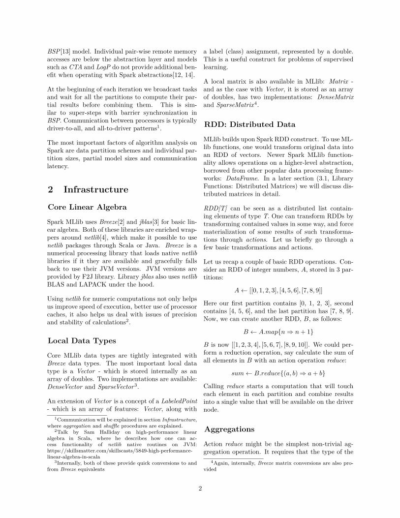
data for a new data partition that is assigned to thisnode (Fig 2).

How expensive is Spark shuffle? On each node,it needs to write a portion of data designated forsome other partition in some separate file, later tobe pulled by the node to which this piece of databelongs. Let us imagine the worst case scenario,where re-partitioning is spreading each previous par-tition into all other partitions. Then on each node,we will have to write all data to disk, and eachnode will have to pull data from each other node -all of the data will be moved and all of the datacached in memory on each node become useless, be-cause now each node has to work with new data.

p1 p2 p3

p1 p2 p3

Figure 2: Shuffle

Shuffle operation is per-formed during many stan-dard RDD operations. Forexample, if we attempt tojoin two RDDs of key/-value pairs on their keys,we are re-partitioning ourdata into a common keypartitioning and thus per-form a shuffle.

To build efficient programs on Spark, it is importantto partition data with consideration of required datatransfers. For example, this is done in treeAggregatedescribed earlier: at each level of the tree, on av-erage only half of the current data gets transferredwhile the other half stays on the same node for fur-ther processing. MLlib implementation is aware ofthis concern.

3 Library FunctionsLet us look at available MLlib functionality in de-tail. This section roughly follows MLlib’s core lowerlevel mllib package organization. We will go throughmost of the library functionality, discuss implemen-tation details and comment on notable features,strengths and limitations of implementation, mainlyfocusing on parallelization and scalability.

3.1 Distributed Matrices

Package linalg.distributed contains some imple-mentations of distributed matrices4. The packageprovides a root interface for distributed matrices:

4org.apache.spark.mllib.linalg.distributed

3

DistributedMatrix. For the remainder of this sec-tion, let us consider a m × n matrix M with ele-ments vij , column vectors c1, c2, ..., cn and row vec-tors r1, r2, ..., rm.

We use RowMatrix to partition matrix data into rowvector ranges: an RDD of row vectors ri. To block-partition the matrix we use BlockMatrix. Sometimesit is convenient to use CoordinateMatrix to constructdistributed matrices from distributed matrix entries(i, j, vij). CoordinateMatrix provides methods to con-vert itself into RowMatrix or BlockMatrix forms.

RowMatrix is the workhorse of Spark distributed ma-trix computations. Typically, distributed operationsare implemented for RowMatrix and operations onother implementations would first convert to Row-Matrix and then reference these implementations.

All of the following implementations are for RowMa-trix, with the exception of eigenvector finding anddistributed matrix multiplication. Eigenvectors canbe computed for a matrix without having it material-ized, i.e. we only need to provide a function that willcalculate products of this matrix by some input vec-tor, and so we do not need to actually have any RDDrepresenting this matrix. Distributed matrix multi-plication is implemented only for BlockMatrix form.Let us look at matrix operations in more details.

Gram Matrix

Calculation of Gram matrix

G = M†M, s.t. Gij = 〈ci, cj〉

is also parallelizable. This is done by aggregationof

∑mi=1 r

†i ri over all rows ri. As with most other

computations on arrays, under the hood, each ma-trix/vector operation is performed by BLAS routines.One Spark job will compute Gram matrix and makeit available on the driver node. Each worker node willhave to use O(n2) space to store intermediate com-puted data and communicate it during aggregationstep. Aggregation results in a single local matrix onthe driver node.

Again, just as with eigenvector search, this meansthat materialization of Gram matrix through thiscomputation is not scalable in the number of columns,but it is scalable in the number of rows. For bothof these distributed operations, parallelization acrossrows before aggregation seems to be optimal: eachworker node is busy computing partial results forsome partitions.

Eigenvectors

In Spark MLlib, finding eigenvectors is possible onlyfor symmetric matrices with real values. Calcula-tion is done with Arnoldi iterations, provided byARPACK1. The materialized matrix itself is usuallynot necessary, only the callback function that com-putes its multiplication by a vector. This allows fordistributed processing where multiplication operationis performed in parallel by worker nodes and the re-sults from each partition can be associatively aggre-gated on the driver node. However, since the iter-ations are performed locally on the driver node (allintermediate data is stored locally), this method stillrequires space of 4n(k + 1) double values on a sin-gle node, where n is the number of columns and k isthe number of leading eigenvalues that was requestedto be computed. This computation is scalable in thenumber of rows, but not in the number of columns.

Singular Value Decomposition

Let’s assume we want to find SVD decomposition

M = UΣV †

where Um×k and Vn×k are orthogonal matrices andΣk×k is a diagonal matrix. To do this, we find eigen-vectors of

M†M = V Σ2V †

yielding V and Σ, of dimensions n × k and k × krespectively, which allow them to completely fit inmemory for smaller n and k values. Then we can alsocompute U of dimension m × k, which typically willnot fit in memory on a single machine and needs tobe distributed, since m is the dimension representingthe number of rows in the RowMatrix representation.

Depending on how large n and k (number of valuesto keep) are, singular value decomposition will be cal-culated differently. If n is small (less than 100), or ifk is larger than n/2 and n is not bigger than 15,000threshold, let us call this condition for local eigen-value computation, then we compute Gram ma-trix G = M†M in distributed fashion once, as shownabove, and obtain a local matrix G. Then if k is lessthan n/3, we compute its eigenvectors locally, as ex-plained above, using ARPACK. If k is greater thanor equal to n/3, we use BREEZE method to com-pute SVD directly using Gram matrix multiplicationcallback function2.

1More information on Arnoldi iterations and ARPACK soft-ware can be found in [8, 7, 6].

2BREEZE uses LAPACK for this operation

4

If on the other hand, if condition for local eigen-value computation doesn’t hold, then we avoid ma-terializing Gram matrix, and instead, iteratively com-pute eigenvalues of M†M , in each iteration1 we com-pute

v 7→M†Mv

in parallel, transmitting data with size only on theorder of O(n). As with eigenvalue search and Grammatrix computation, this will require a new map/ag-gregate job and the associated communication costsin each iteration.

SVD computation in Spark MLlib scales (distributescomputation) well with number of rows (m), but notas well with the number of columns (n): one mustbe aware that a vector of size n must fit in mem-ory. For example, when SVD is applied to a term-document matrix, number of columns (typically num-ber of terms) should be trimmed down to somethingmanageable on a single machine - e.g. 10K2.

Covariance Matrix

Treating each row vector ri as an observation with mvalues, we can use Gram matrix to calculate covari-ances. Gram matrix is calculated in parallel and ismade available on the driver node. In a distributedway, we also compute means for each column:

µi =∑

k

cki /m

and use the formula

Cov(X,Y ) = E[XY ]− E[X]E[Y ]

to compute covariances without care for precision (noBLAS here). This makes Spark covariance computa-tion for RowMatrix numerically unstable and MLlibusers should be aware of this.

Principal Component Analysis

Spark MLlib calculates PCA by computing SVD forcovariance matrix locally on the driver node3 and tak-ing the desired number of singular values. Here we in-herit numerical instability of covariance matrix com-putation operation, which is described above. Also,

1Arnoldi iteration method. Local computations are han-dled by ARPACK, we only provide a callback function thatwill compute v 7→ M†Mv in parallel and return computedmultiplication back to eigenvector computation routine.

2example of this is shown in book Advanced Analytics withSpark[21]

3Breeze over LAPACK

here we cannot arbitrarily scale with the number ofdimensions because we have to perform this on a sin-gle node. Principal component analysis and singularvalue decomposition are the main methods for dimen-sionality reduction in Spark MLlib.

Pair-wise Cosign Similarities

This operation calculates cosine similarities betweenall pairs of columns. It performs an algorithm DIM-SUM (dimension-independent similarity computationusing MapReduce). The algorithm effectively per-forms computations on sampled data4.

Local Matrix Multiplication

Spark MLlib support transformation of a given dis-tributed matrix M , by multiplication with a local(not-distributed) matrix A on the right side: MA.Matrix A is serialized and broadcast to all workernodes and each portion of the resulting matrix MAis calculated by worker nodes independently, result-ing in a new RowMatrix.

Distributed Matrix Multiplication

Distributed matrix multiplication is not available forRowMatrix, but it is implemented for BlockMatrixform. Ideally, we want this to be scalable not onlyin the number of rows, but also in the number ofcolumns. This requires us to partition in both di-mensions, which is achieved with BlockMatrix5.

This multiplication between two block matrices Mand N requires that they have compatible parti-tioning schemes: number of columns in blocks ofM must match the number of rows in blocks ofN . Co-grouping blocks of A and B by (iA, jB , k),where iA are row indices of blocks in A, jB arecolumn indices of blocks in B, k runs throughcolumn indices of A (same as row indices of B),and reducing over all k to common key (iA, jB), wecome up with blocks of AB. Co-grouping requiresa shuffle step6, where each target block (iA, jB)of AB receives a row of blocks from A and acolumn of blocks from B: so in total from aboutO(numColBlocksA + numRowBlocksB) partitions,which makes the total communication size during

4Description of DIMSUM algorithm can be found here:http://arxiv.org/abs/1206.2082

5Current published version of Spark MLlib (1.3) providesonly block partitioned version, in future it might provide ma-trices with other partitioning, such as cyclic or hybrid.

6worst case is all-to-all communication

5

shuffle O(numColBlocksA × numRowBlocksB ×(numColBlocksA + numRowBlocksB) ×colsPerBlockA × rowsPerBlockB . This furthersimplifies to

O(2n3A/colsPerBlockA)

double values transmitted between nodes1.

This shows the trade-off between communication sizeand computation size on nodes: we can decrease com-munication size by increasing the number of columnsper block in A (colsPerBlockA), and in doing so in-crease the computation and memory requirements oneach node: extreme case is a non-partitioned matrix,where all computation is performed on a single node.On the other hand, we can allocate smaller computa-tion work on individual nodes by decreasing the blocksize (in this case columns per block in A), allowingfor bigger communication size during shuffle phase.

3.2 Convex Optimization

Many ML problems can be viewed as convex opti-mization problems. MLlib provides parallel imple-mentations for two basic optimization algorithms:SGD and L-BFGS[10, 11].

Package optimization2 contains a trait Optimizer,which requires only one method

optimize(RDD[(Double, V ector)], V ector) : V ector

This method takes labeled input data points(RDD[(Double, V ector)]) and an initial weights vec-tor, and performs an optimization yielding the result-ing weights vector.

Out of the box MLlib provides two optimizers:Stochastic Gradient Descent and L-BFGS.

Stochastic Gradient Descent

For SGD, we provide a method that calculates gra-dients (trait Gradient) and a function that updatesthe weights (trait Updater), possibly adding gradientcontributions from some regularization3. Let us lookat Gradient and Updater in more detail:

1it is likely that there will be multiple partitions will beallocated per node, so this is worst case scenario, where eachpartition is computed on a distinct worker node. Also it in-cludes the blocks that this partition already has - its own block,but this is not important asymptotically.

2org.apache.spark.mllib.optimization3In future, Updater will be split into Regularizer and

StepUpdater

Gradient: given a labeled data point and weightvector, calculate gradient and weight vector update.MLlib provides 3 implementations: Hinge, LeastSquares, Logistic.

Updater : given a calculated loss gradient, calculatesthe next iteration of model vector, by adding regu-larization gradient and adjusting for step size. Outof the box, MLlib comes with implementations withno-regularization or regularizations based on L1, L2.

SGD computation follows the iterative executionmodel described earlier4. We start with a guess for aweight vector. Then, in each iteration, we broadcastthat current weights vector along with the gradientcomputation. Using this information, we computegradient contributions from data points in each par-tition. We perform this calculation on a subset ofavailable data in partition, facilitated by RDD sam-pling functionality5. At the end of the iteration, par-tial gradients are aggregated on the driver node andan Updater is applied, where additional regularizergradients are added, thus yielding a new estimate forthe weights vector.

Iteration termination condition is simply the numberof iterations, with default value of 100.

L-BFGS

L-BFGS is a quasi-Newton method that in eachiteration uses second-order adjustment to find di-rection towards improved guess and hence con-verges faster than SGD, which only uses first-order approximation[10]. Inverse Hessian (matrix ofsecond-order partial derivatives) is not materialized,but instead is approximated using previous gradientevaluations.

Breeze drives iterations of the calculation, andthrough callback functions interacts with Spark whenwe need to calculate loss value and gradient for agiven weight vector in parallel.

It is preferred to use L-BFGS because of its fasterconvergence, however some current (1.3) Updater im-plementations that were originally designed for SGDare not suitable for L-BFGS (e.g. L1) [1].

4see section Execution Model5RDD.sample(...) method

6

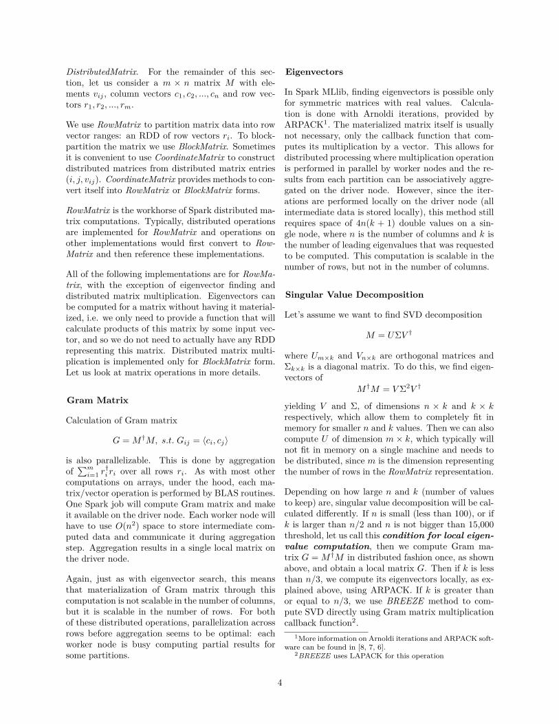
3.3 Generalized Linear Model

Generalized linear algorithms can be solved as convexoptimization problems. We can pick an optimizer,provide it gradient computation method and regular-ization function, and solving that optimization prob-lem, we get solutions to regression problems.

Algorithm Loss RegularizerLinear Regression Least Squares NoneLogistic Regression Logistic L2Ridge Regression Least Squares L2Lasso Regression Least Squares L1

Linear SVM Hinge L2

Figure 3: Generalized Linear Algorithms

Combinations of the provided gradients and regular-izations automatically give us some useful algorithmsfrom the Generalized Linear Algorithms family in theform of stochastic gradient descent (Fig 3).

Spark MLlib 1.3 provides SGD implementations ofthese algorithms. For logistic regression, it also pro-vides L-BFGS implementation.

3.4 Classification Algorithms

Let us look at available classification algorithms.Most of them rely on generalized linear algorithms, asexplained earlier. Some rely on tree-based methodsand we will discuss them separately in section Treemethods.

In package classification1 we have a trait Clas-sificationModel which predicts a class for a givenvector. There are three implementations that aretrained with Logistic Regression, Linear SVM orNaive Bayes. As we have seen earlier, Logistic Re-gression and Linear SVM are members of generalizedlinear algorithms family. MLlib provides their imple-mentations with SGD. In addition to that, we alsohave L-BFGS implementation for logistic regression.

These generalized linear model classifications supportonly 2-class classification, which is a major drawbackfor users. It is possible to reduce the problem of mul-ticlass classification to combinations of binary classi-fiers with schemes such as one-vs-all, or one-vs-one, orothers. Work is currently under way in ML pipelineAPI2 to introduce generic multiclass to binary reduc-

1org.apache.spark.mllib.classification2ML pipeline API will be discussed in section ML Pipeline

API

tion schemes. Tree-based methods and Naive Bayessupport multiclass classification.

Provided Naive Bayes algorithm implementation isfor a Multinomial Naive Bayes[9] model with proba-bility of a vector x = (tj) to belong to class Ci equalto:

p(Ci|x) = p(Ci)∏

j

p(tj |Ci)

We compute p(Ci) and p(tj |Ci) in parallel, by scan-ning through all data points and collecting totals,and thus deducing the frequencies, which are usedas probability estimates. Transferred data is on theorder of O(m×P ), where m is the number of featuresand P is the number of partitions. This algorithm im-plementation treats feature values as counts and re-quires that all values of all features are non-negative.

MLlib classification algorithms support only linearkernels, which is a considerable limitation for manyapplications. Primary reason for this is that non-linear kernels are difficult to parallelize. This canbe (only) partially mitigated by introducing featureinteractions. Also, as mentioned earlier, a rich setof multi-class decision-tree based classification algo-rithms is also provided in Spark MLlib.

3.5 Regression Algorithms

Most regression algorithms3, with the exception oftwo, come from the above-mentioned generalized lin-ear models and all are implemented with SGD: Lin-ear Regression, Lasso/Ridge Regressions. Withinthe same package, an additional regression algorithmis provided: Isotonic Regression. Outside of thispackage, we have decision tree-based regression al-gorithms.

MLlib isotonic regression is implemented using paral-lelized pool adjacent violators (PAV) algorithm andis available only for one-dimensional feature vectors.Sequential PAV implementation and parallelizationare described in [15, 16].

3.6 Tree Methods

Spark MLlib provides several tree-based classificationand regression algorithms in package tree4, whichis probably one of the more complicated algorithmpackages in core MLlib today and also could be onethe most useful for classification and regression prob-lems. Two main algorithms are ensemble algorithms

3Package org.apache.spark.mllib.regression4org.apache.spark.mllib.tree

7

that are composed of one or more simple decisiontrees: Random Forest and Gradient Boosted Trees.

Tree algorithms are driven through configuration ob-jects of class Strategy or BoostedStrategy, where userscan specify numerous algorithm parameters allowingfor a great deal of flexibility.

For example, there are abstractions Impurity andLoss associated with tree algorithms. Trait Impu-rity captures the score of class purity used in calcu-lation of information gain, for example, during treegrowth stage when we perform decision node splits.Three implementations are provided which are basedon variance, Gini, and entropy. Trait Loss is usedto communication loss function in Gradient BoostedTrees, and has three implementations: LogLoss, Ab-soluteError and SquaredError. Then, there are ab-stractions for the type of a feature (categorical orcontinuous), quantile strategy, ensemble combiningstrategy, algorithm type (classification or regression),and so on - a modular design allowing many compo-nent combinations.

Base Decision Tree Algorithm

A base single decision tree algorithm functionality isimplemented in an object DecisionTree. It providesa common shared implementation of fitting one de-cision tree that is used by both Random Forest andGradient Boosted Trees algorithms.

Two important methods here are: findSplitsBins,which picks splits for all features taking into accountthe type of features (e.g. categorical or continu-ous) and the task at hand (regression, binary classi-fication, multiclass classification) and findBestSplits,which finds the best splits for given nodes. OperationfindSplitsBins works with a sample of input data forcontinuous value features and safely handles categor-ical data. This operation is scalable. With findBest-Splits we pick best splits at each tree node in parallel.

Random Forests

Random Forest is an ensemble algorithm that is com-posed of one or more simple Decision Trees[17], whereprediction is based on majority vote or an averagevalue of predictions of all decision trees in the en-semble. It can be used for both classification andregression.

We start by picking sub-samples and feature setsfor each tree in the ensemble. Then we distribute

the recursive computation of best splits in all trees.To reduce computation needed, we perform splits onbinned data where possible. At the end of this dis-tributed tree construction, we have an ensemble oftrees that is ready to do predictions.

When we increase the number of trees in random for-est (e.g. to reduce variance of our model), or just addmore training data, we are able to evenly distributethe computation load across all cluster nodes, whichmakes it a good choice for large problems.

Gradient Boosted Trees

Gradient Boosted Trees give us a different way ofcombining individual decision trees. We build upa sequence of smaller trees with boosting method:each new tree contributes a little bit of new in-formation to the final decision, that previous treesmisclassified[18]. This is done by increasing theweight of those misclassified data points at each iter-ation (boosting of some weights).

With gradient boosted trees, each tree is smaller thanin random forest, but we need to build up treessequentially. Calculation of loss function and re-weighting is done in parallel, which helps with paral-lelization of each individual iteration.

3.7 Clustering Algorithms

MLlib provides four clustering algorithms: K-means,Latent Dirichlet Allocation, Gaussian Mixture, andPower Iteration Clustering. K-means and Gaussianmixture algorithms find more general usages, whilepower iteration clustering and latent Dirichlet allo-cation are associated with graph and document datarespectively.

K-means

In K-means algorithms, we pick some initial set ofcluster centers and in each iteration we compute abetter set of centers. This is done through relabelingthe data points by picking the closest of the currentcenters and picking class means of data points, basedon the new class assignments, as our new centers.Error function that we care about in K-means algo-rithms isWithin Set Sum of Squared Error (WSSSE).

Algorithm runs in the typical [broadcast, computepartials, collect, ...] pattern that was described insection Iterations, making this computation trivially

8

parallelizable and scalable1.

Users can control parameters such as number of it-erations, convergence threshold, number of times tore-run algorithm. The last parameter is importantbecause there is no guarantee of a single minimum.

Gaussian Mixture

Generalization of K-means algorithm, Gaussian Mix-ture Model, is implemented in Spark MLlib. Gaus-sian Mixture Model objects of class GaussianMixture-Model (GMM) are encoded by one array of weightsand one array of multivariate Gaussian objects, whichthemselves are pairs of two other items: one doublerepresenting mean, and one local matrix representingcovariances.

Gaussian Mixture algorithms tries to find the setof Gaussian distributions of sub-populations withinthe main population sample that we are workingon. It does so with Expectation Maximization (EM)algorithm[19], where at each step we try to come upwith a better estimated set of Gaussians.

Input data is in the form of RDD of local vectors.First step is to convert local vectors into Breeze vec-tors and cache them in memory. This is the datathat our iterations will run against. We pick a smallrandom sample of data for each cluster and calculatemeans and the covariance matrix for chosen clusters- this will serve as our initial guess.

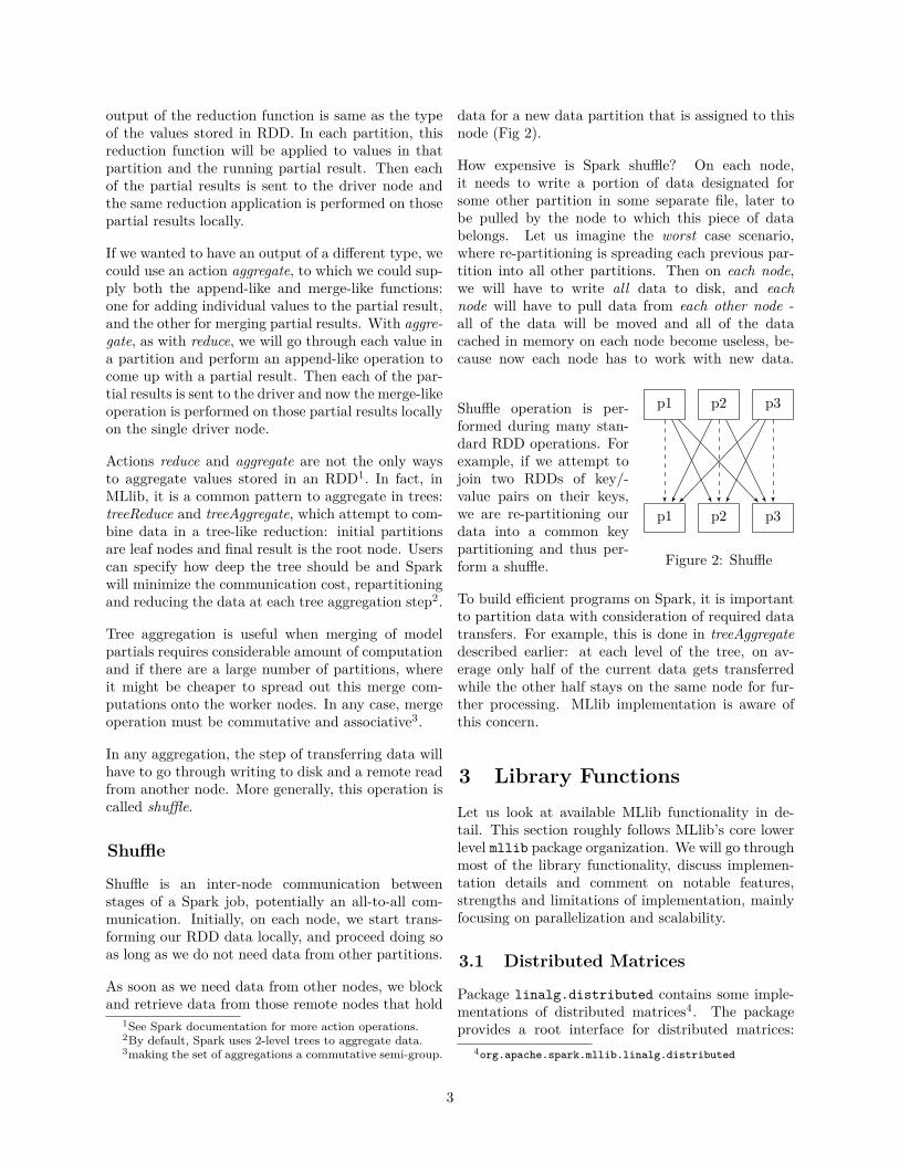
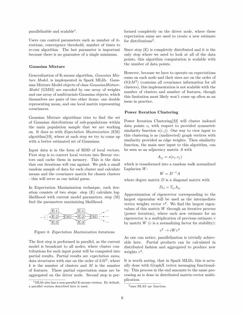
In Expectation Maximization technique, each iter-ation consists of two steps: step (E) calculate log-likelihood with current model parameters, step (M)find the parameters maximizing likelihood.

...E:1E:2E:3

ME:1E:2E:3

M.........

Figure 4: Expectation Maximization iterations

The first step is performed in parallel, as the currentmodel is broadcast to all nodes, where cluster con-tributions for each input point will be computed intopartial results. Partial results are expectation sums,data structures with size on the order of kM2, wherek is the number of clusters and M is the numberof features. These partial expectation sums are beaggregated on the driver node. Second step is per-

1MLlib also has a non-parallel K-means version. By default,a parallel version described here is used.

formed completely on the driver node, where theseexpectation sums are used to create a new estimatefor distributions2.

Since step (E) is completely distributed and it is theonly step where we need to look at all of the datapoints, this algorithm computation is scalable withthe number of data points.

However, because we have to operate on expectationssums on each node and their sizes are on the order ofO(kM2) (contains all covariance information for allclusters), this implementation is not scalable with thenumber of clusters and number of features, thoughthis limitation most likely won’t come up often as anissue in practice.

Power Iteration Clustering

Power Iteration Clustering[22] will cluster indexeddata points vi with respect to provided symmetricsimilarity function s(i, j). One way to view input tothis clustering is as (undirected) graph vertices withsimilarity provided as edge weights. Then similarityfunction, the main user input to this algorithm, canbe seen as an adjacency matrix A with

Aij = s(vi, vj)

which is transformed into a random walk normalizedLaplacian W :

W = D−1A

where degree matrix D is a diagonal matrix with

Dii = ΣjAij

Approximation of eigenvector corresponding to thelargest eigenvalue will be used as the intermediatevertex weights vector vᵀ. We find the largest eigen-values of this matrix W through an iterative process(power iteration), where each new estimate for aneigenvector is a multiplication of previous estimate vby matrix W (c is a normalizing factor for stability):

vᵀ → cWvᵀ

As one can notice, parallelization is trivially achiev-able here. Partial products can be calculated indistributed fashion and aggregated to produce newweights vᵀ.

It is worth noting, that in Spark MLlib, this is actu-ally done with GraphX vertex messaging functional-ity. This process in the end amounts to the same pro-cessing as is done in distributed matrix-vector multi-plication.

2uses BLAS syr function.

9

Convergence condition used is on the rate of changein differences between successive weight vector esti-mates vᵀ - algorithm can be stopped when accelera-tion of changes is small enough[22].

Multiple iterations of this algorithm lead to weightassignments vᵀ that are then passed into K-meansalgorithm for separation into clusters, also a paral-lelized procedure.

Latent Dirichlet Allocation

Just as we used iterative Expectation Maximizationtechnique to find the best fitting mixture of Gaus-sians, we can find best fits for topics in documents,when looking at both documents and topics as bag-of-words objects.

In Spark MLlib, search for the best fitting topicmodel with Latent Dirichlet Allocation is reducedto an optimization problem. Two implementa-tions are provided - one is based on ExpectationMaximization[24], which uses GraphX, and the otheris an online algorithm that operates on samples ofdata and performs online variational Bayes LDA[23].

The first optimization algorithm creates a bipartitegraph representing term-document relationships. Oneach vertex we store an array that contains informa-tion about topic counts (array of doubles). It startswith random soft assignments of tokens to topics andrepartitioning of the graph, so that edges are groupedby document. Then we perform typical expectationmaximization iterations, where at the end of each it-eration we have updated topic counts on each vertex.

The online optimization algorithm processes a smallsample of the corpus on each iteration, and updatesthe term-topic distribution adaptively for the termsappearing in that sample. As input data, it takesan RDD of document IDs along with a vector ofterms for that document (bag of words representa-tion) and doesn’t modify it for processing, unlike thefirst graph-based EM implementation.

Both of the algorithms parallelize well with the num-ber of documents. As for the number of terms, itappears that the second implementation has to keepdata structures with size on the order of the numberof terms in memory and thus can present a scalabilitybottleneck.

3.8 Recommendation Algorithms

Currently, Spark MLlib provides only one recommen-dation algorithm - Alternating Least Squares (ALS)- it is based on the collaborative filtering technique,where two sides (factors) of recommendation (e.g.users and products) are hypothetically connectedthrough a set of unobserved (latent) factors[20].

IfA = Aij is such a matrix with each row representingsome user’s purchases and each column representingsome product purchases, then we propose that it isa product of two matrices X and Y †, where both Xand Y have k columns:

A = XY †

This means that somehow we can capture informa-tion about users and products individually in a vec-tor in some k-dimensional space. It could be, for in-stance, a preference for some genre of music, or someother topic which is not openly given in input data.Then generated recommendations work as similaritymeasure between users and products in this discov-ered basis, e.g. inner product (cosine similarity):

Rec(usera, prodb) = ΣiXaiYbi

Typically, input data to this algorithm is a large andsparse matrix. For example, if we look at users andtheir purchased or rated products, users could be rep-resented by rows and products by columns: each rat-ing (explicit information - user rated the product) oreach purchase (implicit information - we assume thatuser liked the product to some degree) is representedby an entry in this sparse matrix.

When we supply an input RDD of all entries in thismatrix A (e.g. ratings), we iterate a fixed number oftimes, by alternating computation of X from A andY , and Y from A and X, using the familiar minimumleast squares computation:

X = AY (Y †Y )−1

andY † = (X†X)−1X†A

making this training procedure scalable and well-parallelized.

For the final computed model, Spark MLlib imple-mentation creates an object of type MatrixFactoriza-tionModel, which is a model that represents the resultof matrix factorization XY †.

10

Provided algorithm can be trained with implicit rat-ings, e.g. user X purchased product A, or explicitratings, e.g. user X rated product A at 4.5/5.0. Bothversions run similar iterations under the hood.

One scalability limitations are that the current im-plementation supports only IDs (number of rows/-columns) of type 32-bit integers. Another drawbackis that the model is large, it is a distributed matrixof size on the order of the number of users and prod-ucts. This might be a concern for real-time analyticsapplications, because in order to produce recommen-dations, one will need to have this model in memoryon all nodes and run a Spark job to come up with rec-ommendations of products for a given user, or usersfor a given product.

3.9 Frequent Pattern Mining

Spark MLlib provides a parallel implementationan algorithm for mining frequent item-sets: FP-growth[25, 26]. Input data comes in as an RDD ofarrays of items (arbitrary type of items). Initially,we calculate individual item frequencies by simplyusing a reduceByKey operation. Then we utilize aspecialized suffix-tree data structure, FP-Tree, to runthrough the elements of the RDD and build all asso-ciation frequencies. This ends up being performedcompletely in parallel. The only possible bottleneckis the size of the tree, which must completely fit inmemory on any individual node.

3.10 Feature Engineering

Besides standard ML algorithms, we are also pro-vided several feature engineering tools: Word2Vec,TF/IDF, feature normalizer/scaler, feature selection.Standard scaler will scale and shift data to make itsmean zero and standard deviation of unity. Normal-izer will scale the values of a vector to make its normunity. Chi-squared feature selector will perform Pear-son’s test for independence between categorical fea-tures and label, and select only the features closest tothe label. All these three functionalities are triviallyparallelized. Let us look at Word2Vec and TF/IDF.

Word2Vec

Given a set of documents, this procedure will create avector representation of each occurring term, in sucha way that "similar" terms will be closer in this vectorspace. The concept of similarity between terms hereis when another term could replace this term giventhe context, something similar to the concept of a

synonym.

Spark MLlib implementation uses skip-gram modelwith hierarchical softmax method. Algorithm willperform a series of iterations, where in each itera-tion we will go through all sentences and update twoarrays of size equal to the vocabulary size (number ofall terms).

During processing of each sentence, we go througheach word and for each word we will need to loopover log(|V ocabulary|) elements in the Huffman en-coding (tree) of all terms. This is the hierarchicalsoftmax portion used to calculate conditional termprobabilities.

Assuming each node can hold two arrays and a treecontaining data for each term in vocabulary, then therest is easy parallelized along with input sentencesdistribution.

TF/IDF

Term frequency-inverse document frequency is calcu-lated in two parts. First we need to compute termfrequencies and then we also need to compute inversedocument frequencies. In Spark MLlib, hashing isused to generate a unique id for a term. This helpswith parallelization, as no single map of term indicesis necessary, but this comes at a cost of hash colli-sions. Term frequencies are calculated trivially witha single pass over sentences, while inverse documentfrequencies are calculated in two passes: one to countoccurrences, and second to normalize them.

3.11 Other Functionality

Let us just mention several useful functionalities pro-vided in Spark MLlib that are naturally parallelizedor do not require parallelization.

Basic Statistics

Summary statistics can obviously be calculated inparallel. Kernel density estimation is possible ongiven limited set of points for which it needs to becomputed. Here we simply aggregate contributionsfrom all elements in the dataset at these points.

It is possible to generate RDDs with random num-bers from certain distribution families, but it is notclear how to properly align it with existing RDD data.Random RDD creation basically works by shipping aspecific random number generator to partitions and

11

modifying its seed using partition id.

Pearson and Spearman correlations are provided:Pearson correlation is computed from covariance ma-trix generated from rows of a RowMatrix of incomingdata, while in Spearman correlation computation, wefirst construct grouped ranks by iterating over all val-ues, and then calculate Pearson correlation.

Stratified sampling is possible by providing desiredclass distributions and going through each record de-ciding whether to include it in the sample or not. Ex-act version of this sampling requires more processing,but is still parallelized.

Chi-squared independence test is parallelized - only asingle pass through distributed input data is neces-sary. Intermediate data will be aggregated to con-struct contingency tables used in further processing.

Evaluation Metrics

Several evaluation metrics are available for models:BinaryClassificationMetrics, MulticlassMetrics, Re-gressionMetrics, RankingMetrics. All of metrics func-tions are naturally parallel in nature, since they usesome computed model to calculate predictions foreach point in the data set in parallel.

PMML Export

Spark MLlib provides a trait PMMLExportable to des-ignate models that can be exported to PMML 1. Im-plementation of PMML export is a very recent devel-opment and is provided only for a basic set of MLlibmodels. It is currently under development to includemore models. This is performed locally on the drivernode.

4 Streaming SupportOne of the desired qualities in a machine learninglibrary is ability to learn from streaming data.

One special case is models that are built using SGD.Whenever model weights are updated with stochas-tic gradient descent, we can use streaming data totrain this model continuously. Spark MLlib provides

1Quoting from Wikipedia, Predictive Model Markup Lan-guage (PMML) is an XML-based file format developed by theData Mining Group to provide a way for applications to de-scribe and exchange models produced by data mining and ma-chine learning algorithms.

implementation of this sort for binary classification:StreamingLogisticRegressionWithSGD.

For streaming clustering, we have an algorithmStreamingKMeans available in the library.

This is where the list of streaming ML algorithmsprovided by default ends.

5 spark.mlSupport for high-level use of MLlib is provided withspark.ml, which organizes machine learning workwith ML pipelines. By its meta-processing nature,this processing itself does not need to be parallelized,while individual stages of the pipeline will have theirown independent parallelization.

Dataset

Spark ML operates on a ML Dataset, a conceptof data set which is built on top of Spark SQLDataFrame structures that can use custom binaryformats to store columnar data more efficiently.DataFrame performance received a lot of attentionfrom Spark developers, making newer implementa-tions CPU-efficient, cache-aware.

Pipelines

Two main concepts in spark.ml are ML pipeline state-less processing stage types: Transformers and Esti-mators. Transformer stages transform DataFramesinto new DataFrames. For instance, some trans-former stage can apply a model to data and calculatepredictions. Estimator stages take DataFrames andcreate Transformers. An example of this would be alearning algorithm that produces a model that canmake predictions on new input data. A sequence ofTransformers and Estimators forms a Pipeline.

6 ComparisonsLet us briefly discuss how Spark MLlib is similar toor different from some other existing machine learn-ing libraries2. We can analyze and compare alter-natives using the following four axis: availability ofalgorithms, parallelization and distribution of work-load, visualization capabilities, and flexibility.

2A comprehensive review and comparison of all machinelearning frameworks and libraries is not provided here. Insteadonly 4 major alternatives are discussed

12

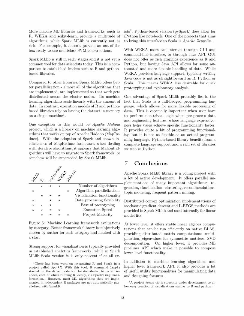
More mature ML libraries and frameworks, such asR, WEKA and scikit-learn, provide a multitude ofalgorithms, while Spark MLlib is currently not asrich. For example, it doesn’t provide an out-of-thebox ready-to-use multiclass SVM constructions.

Spark MLlib is still in early stages and it is not yet acommon tool for data scientists today. This is in com-parison to established leaders such as R and python-based libraries.

Compared to other libraries, Spark MLlib offers bet-ter parallelization - almost all of the algorithms thatare implemented, are implemented so that work getsdistributed across the cluster nodes. Its machinelearning algorithms scale linearly with the amount ofdata. In contrast, execution models of R and python-based libraries rely on having the dataset in memoryon a single machine1.

One exception to this would be Apache Mahoutproject, which is a library on machine learning algo-rithms that works on top of Apache Hadoop (MapRe-duce). With the adoption of Spark and shown in-efficiencies of MapReduce framework when dealingwith iterative algorithms, it appears that Mahout al-gorithms will have to migrate to Spark framework, orsomehow will be superseded by Spark MLlib.

MLlib

R scikit-learn

WEK

AMahout

? ? ? Number of algorithms? ? Algorithm parallelization

? ? ? Visualization functionality? ? ? Data processing flexibility? ? ? Ease of prototyping? ? ? ? Execution Speed

? ? ? ? Project Maturity

Figure 5: Machine Learning framework evaluationsby category. Better framework/library is subjectivelychosen by author for each category and marked witha star.

Strong support for visualization is typically providedin established analytics frameworks, while in SparkMLlib Scala version it is only nascent if at all ex-

1There has been work on integrating R and Spark in aproject called SparkR. With this tool, R command lapplystarted on the driver node will be distributed to to workernodes, each of which running R locally, via Spark’s map trans-formation. However, most ML algorithms that are imple-mented in independent R packages are not automatically par-allelized with SparkR.

ists2. Python-based version (pySpark) does allow foriPython like notebook. One of the projects that aimsto bring this interface to Scala is Apache Zeppelin.

With WEKA users can interact through GUI andcommand-line interface, or through Java API. GUIdoes not offer as rich graphics experience as R andPython, but having Java API allows for some au-tomated and more flexible handling of data. WhileWEKA provides language support, typically writingJava code is not as straightforward as R, Python orScala. This makes WEKA less desirable for quickprototyping and exploratory analysis.

One advantage of Spark MLlib probably lies in thefact that Scala is a full-fledged programming lan-guage, which allows for more flexible processing ofdata. This is especially important when user haveto perform non-trivial logic when pre-process dataand engineering features, where language expressive-ness helps users achieve specific functionality faster.R provides quite a bit of programming functional-ity, but it is not as flexible as an actual program-ming language. Python-based library benefits from acomplete language support and a rich set of librarieswritten in Python.

7 ConclusionsApache Spark MLlib library is a young project witha lot of active development. It offers parallel im-plementations of many important algorithms: re-gression, classification, clustering, recommendations,topic modeling, frequent pattern mining.

Distributed convex optimization implementations ofstochastic gradient descent and L-BFGS methods areprovided in Spark MLlib and used internally for linearmodel fits.

At lower level, it offers stable linear algebra compu-tations that can be run efficiently on native BLAS,providing distributed matrix computations: multi-plication, eigenvalues for symmetric matrices, SVDdecomposition. On higher level, it provides MLpipelines API which make it possible to composelower level functionality.

In addition to machine learning algorithms andhigher level framework API, it also provides a lotof useful utility functionalities for manipulating dataand designing features.

2A project breeze-viz is currently under development to al-low easy creation of visualizations similar to R and python.

13

References[1] Machine Learning Library (MLlib) Guide,

https://spark.apache.org/docs/latest/mllib-optimization.html

[2] Breeze: numerical processing library for Scala,https://github.com/scalanlp/breeze

[3] jblas: linear algebra for Java, http://jblas.org/

[4] netlib: collection of mathematical software,http://www.netlib.org/

[5] Jeffrey Dean and Sanjay Ghemawat, MapRe-duce: Simplified Data Processing on Large Clus-ters, Google, Inc 2004

[6] W.E. Arnoldi, The principle of minimized iter-ations in the solution of the matrix eigenvalueproblem Quart. Appl. Math., 9, pp. 17-29 1951

[7] R.B. Lehoucq, D.C. Sorensen, and C. Yang,ARPACK Users’ Guide: Solution of Large-ScaleEigenvalue Problems with Implicitly RestartedArnoldi Methods SIAM, Philadelphia, 1989

[8] D.C. Sorensen, Implicit Application of Polyno-mial Filters in a k-step Arnoldi method. SIAMJ. Matrix Anal. Appl., 13:357-385, 1992

[9] Naive Bayes in Text Classification http://nlp.stanford.edu/IR-book/html/htmledition/naive-bayes-text-classification-1.html

[10] J. Nocedal Updating Quasi-Newton Matriceswith Limited Storage Mathematics of Computa-tion 35, pp. 773-782. 1980

[11] D.C. Liu and J. Nocedal On the Limited memMethod for Large Scale Optimization Mathemat-ical Programming B, 45, 3, pp. 503-528. 1989

[12] Snyder, Lawrence, Type architectures, sharedmemory, and the corollary of modest potential,Ann. Rev. Comput. Sci 289-317, 1986

[13] Valiant, L. G., A bridging model for paral-lel computation, Communications of the ACM33(8):103-111, 1990

[14] Culler, D. et al, LogP: Towards a RealisticModel of Parallel Computation, Proceedings ofIV ACM SIGPLAN Symposium on Principlesand Practice of Parallel Programming, May 1993

[15] Tibshirani, Ryan J., Holger Hoefling, and RobertTibshirani, Nearly-isotonic regression, Techno-metrics 53.1 (2011): 54-61. 2011

[16] Kearsley, Anthony J., Richard A. Tapia, andMichael W. Trosset, An approach to parallelizingisotonic regression., Applied Mathematics andParallel Computing. Physica-Verlag HD, 1996.141-147. 1996

[17] Breiman, Leo, Random Forests, Machine Learn-ing 45 (1): 5-32 2001

[18] Friedman, J. H., Greedy Function Approxima-tion: A Gradient Boosting Machine., 1999

[19] Dempster, A.P.; Laird, N.M.; Rubin, D.B., Max-imum Likelihood from Incomplete Data via theEM Algorithm., Journal of the Royal StatisticalSociety, Series B 39 (1): 1-38 1977

[20] Koren, Yehuda and Bell, Robert and Volin-sky, Chris, Matrix Factorization Techniques forRecommender Systems, IEEE Computer SocietyPress, J. Computer, 42: 30-37 2009

[21] Sandy Ryza, Uri Laserson, Sean Owen, JoshWills, Advanced Analytics with Spark, O’Reilly,2015

[22] Frank Lin, William W. Cohen, Power IterationClustering, Proceedings of the 27th InternationalConference on Machine Learning, Haifa, Israel,2010

[23] Hoffman, Blei and Bach, Online Learning for La-tent Dirichlet Allocation, NIPS, 2010

[24] Asuncion, Welling, Smyth, and Teh. On Smooth-ing and Inference for Topic Models, UAI, 2009

[25] Han et al., Mining frequent patterns without can-didate generation, Proceedings of the 2000 ACMSIGMOD international conference on Manage-ment of data, 2000

[26] Li, Haoyuan and Wang, Yi and Zhang, Dongand Zhang, Ming and Chang, Edward Y., Pfp:Parallel Fp-growth for Query Recommendation,Proceedings of the 2008 ACM Conference onRecommender Systems, 2008

14