Download - Well-connected Short-sellers Pay Lower Loan Fees: … ANNUAL MEETINGS... · Well-connected Short-sellers Pay Lower Loan Fees: a Market-wide Analysis ... We test two hypotheses: H1)

Well-connected Short-sellers Pay Lower Loan Fees: a

Market-wide Analysis∗

Fernando Chague† Rodrigo De-Losso‡

Alan De Genaro§ Bruno Giovannetti¶

October 1, 2015

Abstract

High loan fees generate short-selling constraints and, therefore, reduce price e�-

ciency. Despite the importance of loan fees, empirical evidence on their determinants is

scarce. Using a market-wide deal-by-deal data set on the Brazilian equity lending mar-

ket which uniquely identi�es borrowers, brokers, and lenders, we are able to construct

a proxy of search costs at the borrower-stock-day level. We �nd that � for the same

stock, on the same day � borrowers with higher search costs pay signi�cantly higher

loan fees. Our results suggest that regulators should encourage the use of a centralized

lending platform to reduce search costs in the lending market.

∗We thank Rafael Benini, Marco Bonomo, Elias Cavalcante, Giulia Iori, Marcos Nakaguma, Pedro Sa�,José Carlos de Souza Santos, Marcos Eugênio da Silva, Leonardo Viana and seminar participants at Uni-versity of São Paulo, Getúlio Vargas Foundation and Insper for their comments and suggestions. We areresponsible for any remaining errors.†Department of Economics, University of Sao Paulo, Brazil. E-mail: [email protected]‡Department of Economics, University of Sao Paulo, Brazil. E-mail: [email protected]§Department of Economics, University of Sao Paulo, Brazil. E-mail: [email protected]¶Department of Economics, University of Sao Paulo, Brazil. E-mail: [email protected]

1

1 Introduction

A short-seller is constrained if the loan fee exceeds the expected fall in the stock price.

High loan fees therefore generate short-selling constraints. Short-selling constraints are not

desirable for two reasons: they cause stock overpricing (Danielsen and Sorescu (2001), Jones

and Lamont (2002), Nagel (2005), Chang et al. (2007), Stambaugh et al. (2012) and Blocher

et al. (2013)) and they reduce price e�ciency (Asquith et al. (2005), Nagel (2005), Cao et al.

(2007), Sa� and Sigurdsson (2011), Engelberg et al. (2012) and Boehmer and Wu (2013)).

Despite these adverse e�ects of loan fees on the stock market, there is sparse empirical

literature on the determinants of loan fees, mostly due to lack of data.1 In this paper we use

a unique data set to show that loan fees depend on borrower search costs.

Loan fees should be close to zero in a frictionless lending market. Lenders have long

investment horizons and do not care about short-term variations in stock prices (D'Avolio,

2002), so that lending a stock for a short period is costless. Competition among lenders

would thus drive loan fees to zero. This is not observed in the data, however. Loan fees vary

substantially over time and can be quite high (D'Avolio (2002), Reed (2013) and Engelberg

et al. (2013)).

Du�e, Gârleanu and Pedersen (2002; hereafter DGP) provides a model that explains

why loan fees can be high. In their model borrowers face search costs that limit the frequency

with which they can �nd lenders, allowing lenders to act as local monopolists and thereby

charge positive loan fees. In this setting loan fees are increasing in borrower search costs.

Kolasinski, Reed and Ringgenberg (2013; hereafter KRR) is the only paper which empir-

ically studies the relationship between loan fees and search costs. They use proxies for search

costs which vary across stocks and time, such as �rm size, bid-ask spread, and measures of

stock concentration among lenders. Consistent with the theoretical predictions in DGP, they

�nd that both loan fee levels and loan fee dispersion are increasing in these stock-speci�c

measures of search costs.2

1The equity lending market in the US and other countries is over-the-counter (OTC), with transactionsusually only visible to the parties involved. As we discuss below, although the Brazilian lending market isalso OTC all loan deals must be registered at BM&FBOVESPA, which acts as the central counterpart. Inthis paper we use the BM&FBOVESPA market-wide data.

2DGP's model does not predict loan fee dispersion, since it includes no heterogeneity among lendersand borrowers. As discussed by KRR, industrial organization models with sequential search produce pricedispersion when there is heterogeneity among investors.

2

However, search costs are not just stock-speci�c: di�erent borrowers should face di�erent

search costs when searching for the same stock. Consider two borrowers, A and B. Borrower

A has very good relationships in the lending market: she is a good client of big brokers who

in turn know many active lenders. By contrast, borrower B is connected to a single broker,

who has few connections to active lenders. These two borrowers will face di�erent search

costs for the same stock.

The main contribution of this paper is to be the �rst to study the relationship between

loan fees and search costs at the borrower level. We test two hypotheses: H1) the higher

the search costs a borrower faces, the higher the loan fees she pays; and H2) the higher the

search costs that borrowers face, the higher the loan fee dispersion among these borrowers.

We �nd strong favorable evidence for both H1 and H2.

Measuring borrower-speci�c search costs is empirically challenging. As the above example

suggests, one has to measure the importance of each lender in the market as well as the

strength of the relationships between borrowers, brokers, and lenders. For that to be possible

one needs to (i) observe all loan deals in the market and (ii) uniquely identify borrowers,

brokers, and lenders over time. The data sets used so far in the literature allow neither (i)

nor (ii).

Our data set enables both (i) and (ii). Every transaction in the Brazilian lending market

is cleared through BM&FBOVESPA, which keeps a record of all loan deals closed in Brazil.

Our data set contains information on the loan quantity, loan fee, investor type, borrower ID,

broker ID, and lender ID for all loan deals in the Brazilian stock market from January 2008

to July 2011.3

We construct our borrower-speci�c measure of search costs based on DGP description

of the lending market dynamics. In a typical transaction, a potential short-seller contacts

her broker asking for a particular stock to borrow. The broker then searches for a potential

lender of the stock. Hence, locating a stock will be easier for a borrower who has good

relationships with brokers that, in turn, have good relationships with active lenders of the

stock.

Based on that, we say that a borrower has low search costs if she is �well-connected� to

3The investor-type variable classi�es borrowers as either �individuals� or �institutions�. The ID variablesin our data uniquely identi�es each market participant and is time-invariant. These IDs are �fake�, i.e.,anonymous.

3

brokers that are �well-connected� to active lenders. We say a borrower is well-connected to a

broker if she is an important customer of the broker. We say a broker is well-connected to a

lender if it is responsible for a high share in the loan deals of the lender. Since our data set

allows us to follow each market participant through time, we are able to compute (a) how

well-connected each borrower is to each broker, (b) how well-connected each broker is to each

lender, and (c) how active each lender is in the lending market of each stock. From (a), (b),

and (c) we calculate the Borrower Connection (BC), a variable that is borrower-speci�c,

stock-speci�c, and varies over time. The BC variable is constructed so that it is high when

the borrower is well-connected to brokers which in turn are well-connected to active lenders

of a stock. BC should therefore be negatively related to borrower search costs.

We perform a number of empirical exercises that relate BC to loan fees. We �rst run

deal-by-deal panel regressions with loan fees on the left hand side and BC on the right

hand side. We �nd that low-connected borrowers pay signi�cantly higher loan fees. We also

allow for nonlinear e�ects by separating borrowers into three groups (high-, medium-, and

low-BC) and comparing the average loan fee in each group. We �nd that borrowers in the

low-BC group pay 14.5% higher loan fees than borrowers in the high-BC group.

Second, we use direct measures of loan fee dispersion (loan fee standard deviation and

range across deals for the same stock) to test whether loan fee dispersion is higher among low

connected borrowers. We �nd that loan fee standard deviation and loan fee range among

borrowers in the low BC-group are respectively 46% and 135% higher than those among

borrowers in the high-BC group.

Lastly, we re�ne the analysis by studying the in-broker variation of loan fees. We run the

same regressions using only deals closed within a single broker � the largest one in terms of

deals. The conclusions are the same as before: we �nd that on the same day, for the same

stock, this single broker intermediates deals with di�erent loan fees which are decreasing in

borrower BC.

Importantly, all results are robust across sub-samples. To account for unobserved bor-

rower speci�c e�ects that may correlate with both BC and loan fees, all regressions are run

within sub-samples of borrowers that share similar characteristics with respect to investor

type, traded volume, and frequency of trades. In doing so, we estimate the e�ect of BC on

loan fees across deals closed by similar borrowers. Considering only institutions, we �nd that

a low-BC institution pays an 8.5% higher loan fee than a high-BC institution. Considering

4

only frequent borrowers, we �nd that a low-BC frequent borrower pays a 10.9% higher loan

fee than a high-BC frequent borrower. Finally, considering only large borrowers, we �nd

that a low-BC large borrower pays a 9.8% higher loan fee than a high-BC large borrower.

The paper closest in purpose to ours is KRR. Using a unique data set involving 12

important lenders in the US market, KRR shows that at high borrowing demand levels

positive shocks to demand result in higher loan fees. They moreover show that the e�ect

of borrowing demand on loan fees is greater for stocks associated with high levels of search

costs, which is consistent with DGP. In doing so KRR inaugurates the empirical evidence of

the e�ects of search costs on loan fees. Our paper continues this investigation. In addition to

stock-speci�c search costs, we �nd that search costs at the borrower level are also important

drivers of loan fees.

Engelberg et al. (2013) also empirically investigates loan fees. They run predictive re-

gressions to explain loan fees conditional on a number of variables such as past loan fees,

institutional ownership, lending o�ers, and the federal funds rate. Their goal is to dynami-

cally evaluate short-selling risks. Prado (2015) tests another implication of the DGP model,

namely that stock prices incorporate expected future lending income (i.e., the loan fee, acting

as a dividend, increases the stock's price). She �nds that institutions buy shares in response

to an increase in loan fees, which is consistent with DGP.

This paper also relates to a more general literature on OTC markets. Du�e et al. (2005)

and Du�e et al. (2007) provide a theory of dynamic asset pricing that directly addresses

search and bargaining in general OTC markets, with the goal of evaluating the e�ects of

search frictions on asset prices. Another set of papers focuses on the �percolation� of infor-

mation which is of common interest throughout OTC markets (Du�e and Manso (2007),

Du�e et al. (2009) and Du�e et al. (2010)). Zhu (2012) also presents a dynamic model

of opaque OTC markets where sellers search for buyers. On the empirical side, Ang et al.

(2013) and Eraker and Ready (2015) study the stock returns of �rms that trade on OTC

markets. Our results suggest that opacity in OTC markets induce important search frictions

that a�ect prices: market participants with higher search costs pay higher prices for the

same asset. Regulators should therefore encourage the use of electronic trading platforms to

reduce opacity and hence search costs in these markets.

This paper is organized as follows. Section 2 explains the Brazilian stock lending market

and describes our data set. Section 3 documents the existence of loan fee dispersion. Section

5

4 speci�es our measure of borrower-speci�c search costs. Section 5 presents the empirical

results. Section 6 exhibits the e�ects of a lending platform on loan fees. Finally, Section 7

presents our concluding remarks.

2 Stock Lending in Brazil

The securities lending market in Brazil is regulated by the Brazilian Securities Commission

(CVM).4 All transactions are mediated by BM&FBOVESPA-registered brokers, who are

responsible for bringing together stock borrowers and stock lenders. All securities listed on

the exchange are eligible for lending. Crucially for us, in Brazil every lending transaction

must be registered in the BM&FBOVESPA lending system. This contrasts with most other

lending markets, which are decentralized and in which data about lending deals are only

partially available.

According to D'Avolio (2002) and Reed (2013), in the US the loan fee is implicitly given

by the �rebate� rate when loans are cash-collateralized. The rebate rate is the interest rate

that the lender pays the borrower in exchange for holding the cash-collateral; it is lower

than the federal funds rate. The higher the di�erence between the rebate rate and the fed

fund rate, the higher the implicit loan fee. If the borrower posts instead Treasury securities

as collateral, she simply pays the lender an explicit loan fee. The average loan fee of an

easily-borrowed stock ranges between 0.05% and 0.25% per year. Stocks with high loan fees

are called specials ; their rebate rates may even be negative. Approximately 9% of stocks are

specials, with an average loan fee of about 4.3% (D'Avolio, 2002).The overall average loan

fee in the US is therefore 0.52%.5

All loan deals in Brazil are collateralized with Treasury securities.6 Hence there are no

�rebate� rates and all loan deals are negotiated in terms of explicit loan fees. In our sample

the average loan fee, including all stocks (both specials and non-specials), is 2.75% per year

4The stock lending market in Brazil has grown substantially. During 2011, the last year in our data set,more than US$ 400 billion were loaned in over 1.4 million transactions, corresponding to one-third of theBrazilian market's total capitalization. In that year 290 di�erent stocks were traded in the lending market.

50.52% = 0.09× 4.3% + 0.91× 0.15%.6The collateral is deposited at BM&FBOVESPA, which acts as the central counterpart to all lending

transactions.

6

� much higher than in the US.

One possible explanation for the higher Brazilian loan fees is the higher stock market

volatility. According to DGP, given the existence of borrower search costs, lenders are able

to charge short sellers a loan fee that is equal to some fraction of the short sellers' expected

pro�t, which should be increasing in the expected volatility of the asset price. Hence the

higher the expected volatility, the higher the loan fee (Engelberg et al. (2013) provides

empirical evidence consistent with this). Indeed, stock market volatility is much higher in

Brazil than in the US. During our sample period (January 2008 � July 2011) the average

implied volatility for the US (VIX) was 17.50% whereas in Brazil it was 23.72% (that is,

about 35% higher).7

The higher Brazilian risk-free rate may also contribute to the higher loan fees. Engelberg

et al. (2013) document that loan fees are proportional to the risk-free rate. Indeed, the ratios

between loan fees and risk-free rates in Brazil and in the US are similar.8

2.1 Data Set

We observe all of the 2,302,360 lending deals closed in the Brazilian stock market from

January 2008 to July 2011. For each lending deal we have information on the loan quantity,

loan fee, borrower type (institution or individual), borrower ID, broker ID, and lender ID.

These ID variables uniquely and anonymously identi�es each market participant and are

time-invariant.

The numbers of distinct borrowers and lenders in the lending market are shown in Table

1. In 2008 there were 17,435 distinct borrowers and 3,471 distinct lenders. The number of

investors increased over the subsequent years: there were 22,166 borrowers and 3,416 lenders

in 2009; 24,809 borrowers and 6,785 lenders in 2010; and 16,515 borrowers and 8,103 lenders

in the �rst seven months of 2011.

[Table 1 about here]

7Astorino et al. (2015) calculates the implied volatility for Brazil.8The ratio in the US is 21% = 0.52%/2.5% (using 2.5% as the average federal funds rates). In Brazil, the

ratio is 25% = 2.75%/10.9% (where 10.9% is the average Brazilian risk-free rate, the Selic rate, during oursample period).

7

We apply two �lters to our data set. First, because the main regressions of this paper

use the standard deviation of loan fees for each stock in each week, we need a su�ciently

large number of loan deals per stock per week. We therefore restrict our sample to liquid

stocks in the lending market. We say a stock is liquid if it was loaned during every week of

our sample. We end up with 55 stocks which jointly account for 1,417,964 loan deals.

The second �lter is as follows. According to Brazilian law the tax treatment of �interest

on equity� di�ers by investor type: individual investors pay a tax rate of 15% while �nancial

institutions are exempt. As a result, on days around the ex-date of interest on equity a tax

arbitrage trade between individuals and �nancial institutions commonly occurs: (i) individ-

uals lend shares to �nancial institutions at a higher loan fee; (ii) �nancial institutions receive

the interest on equity and pay no taxes; (iii) �nancial institutions transfer to individuals

the net value (i.e., excluding taxes) that individuals would receive from interest on equity;

and (iv) individuals then receive a higher loan fee, while �nancial institutions pro�t by 15%

of the interest on equity minus the loan fee. Since loan fees from these arbitrage deals are

arti�cially high, we exclude all loan deals that were closed in a six-day window around the

ex-date. The �nal sample encompasses 1,251,801 loan deals involving the 55 most liquid

stocks.

3 Evidence of Loan Fee Dispersion

Opaque markets are characterized by high search costs. This is the case for the stock

lending market, which is OTC. As discussed by KRR, sequential search cost models predict

that markets with high search costs exhibit high price dispersion. In this Section we show

that the Brazilian lending market has signi�cant loan fee dispersion.

We measure loan fee dispersion as the standard deviation of the annualized loan fee of all

deals for the same stock on a given day. Figure 1 shows the time-series of this variable for

the 4 stocks with the largest number of loan deals in our sample, namely VALE5 (131,441

deals), PETR4 (107,263 deals), GGBR4 (78,916 deals), and BBDC4 (70,311). Each point in

the �gure corresponds to the loan fee dispersion of a given day. As can be seen, dispersion

varies greatly during the period. Days with dispersion around 0.5% p.y. are common for the

four stocks, and the variable often reaches 1% p.y., which is high when compared with the

8

average loan fee levels reported on Table 2 for these stocks (VALE5: 0.47%; PETR4: 0.77%;

GGBR4: 2.19%; BBDC4: 0.54%).

[Figure 1 and Table 2 about here]

Figure 2 and Table 2 show the time-series average of the loan fee dispersion for each stock

in our sample. Stocks are alphabetically ordered. Note that average dispersion is high and

varies across stocks.

[Figure 2 about here]

Figure 3 shows the cross-sectional average of the loan fee dispersion for each day in our

sample. High dispersion is frequent in the Brazilian stock lending market.


4 Borrower-speci�c Search Costs

Our goal is to relate (i) the loan fee that a borrower pays to (ii) the search cost she faces when

searching for the stock in the lending market. As shown by KRR, loan fee level and dispersion

are increasing in various proxies for search costs. The proxies KRR use, however, are �rm-

speci�c (market capitalization, liquidity, and the fragmentation of its share lending market)

and do not completely capture search costs at the borrower level. Our main contribution is

to use a borrower-speci�c proxy for search cost.

Our measure of search cost relies on the idea that the stock lending market is a "relationship-

based market", as discussed in DGP and KRR. The typical lending transaction proceeds as

follows. The borrower communicates her broker(s) that she is looking for a particular stock

to borrow. The broker then has to search for a potential lender of the stock.

9

Based on such a dynamics, we assume that a borrower has low search costs if she is

�well-connected� to a broker who in turn is �well-connected� to active lenders. A borrower is

well-connected to a broker if the borrower is an important customer of this broker. A broker

is well-connected to a lender if the broker accounts for a high share of the lender's loans.

We explain with an example. Investor I wants to borrow shares of stock XYZ. Investor

I frequently borrows stocks (from any �rm) with the intermediation of Broker B. Broker

B is in turn responsible for a large share of the loans that Lender L makes (with respect to

all stocks loaned by Lender L). Lender L is an active lender of stock XYZ. Will Investor I

face high search costs in this case? We suppose not. In contrast, Investor I will face higher

search costs if (i) Investor I is not an important client of Broker B and/or (ii) Broker B is

responsible only for a small share of the loans that Lender L makes and/or (iii) Lender L is

a small lender of stock XYZ.

Since our detailed data set allows us to follow each market participant through time,

we are able to compute (a) how well-connected each borrower is to each broker, (b) how

well-connected each broker is to each lender, and (c) how active each lender is in the lending

market of each stock. We use (a), (b), and (c) to calculate the search cost of each borrower.

We now explain the details of this calculation.

4.1 Broker Reach

To calculate the ability of broker i to locate a speci�c stock s to borrow on day t, which

we call BrokerReachi,s,t, we follow three steps. First, we measure the importance of each

lender j in the lending market of stock s on day t as

LenderImportancej,s,t =sharesj,s,t

total sharess,t,

where sharesj,s,t is the number of shares lent by lender j of stock s during the 90-day period9

previous to day t, and total sharess,t is the total number of shares of stock s that were loaned

in the same period.

9The 90-day window was arbitrarily chosen and the �rst to be considered. All results are robust to 60-dayand 120-day windows and are available upon request.

10

We then quantify the strength of the relationship of broker i with lender j on day t as

BrokerLenderRelationi,j,t =dealsi,j,t

total dealsj,t

where dealsi,j,t is the total number of loan deals closed, considering all stocks, between broker

i and lender j in the 90-day period previous to day t, and total dealsj,t is the total number

of loan deals made by lender j in the same period.

The assumption here is that if broker i recently closed many loan deals with lender j, then

they have a good relationship. Note that measured this way the strength of the relationship

between broker i and lender j is not stock-speci�c.

Finally, the ability of broker i to locate stock s on day t is given by

BrokerReachi,s,t =J∑

j=1

LenderImportancej,s,t ×BrokerLenderRelationi,j,t

where J is to total number of lenders.

BrokerReachi,s,t will be high for a broker that, on day t, has good relationships with

important lenders of stock s. By construction, the cross-broker sum

I∑i=1

BrokerReachi,s,t

is equal to one for any s = 1, ..., S and every t = 1, ..., T .

4.2 Borrower Connection

If a borrower has good relationships with brokers with high BrokerReach on stock s, it

should be easy for her to �nd the stock. That is, this well-connected borrower will have low

search cost for this stock. Based on this idea we calculate the connection of borrower k with

respect to stock s on day t , which we call BorrowerConnectionk,s,t , in two steps.

We �rst quantify the strength of the relationship between borrower k and each broker i

on day t as

BorrowerBrokerRelationk,i,t =dealsk,i,t

total dealsi,t

11

where dealsk,i,t is the number of loan deals (considering any stock) between borrower k and

broker i in the 90-day period previous to day t, and total dealsi,t is the total number of loan

deals made by broker i in the same period.

The connection of borrower k with respect to stock s on day t is then

BCk,s,t = 100×

(I∑

i=1

BrokerReachi,s,t ×BorrowerBrokerRelationk,i,t

)

We multiply the right-hand side by 100 so that BCk,s,t is expressed in percentage points.

By construction, for any s = 1, ..., S and at any t = 1, ..., T the sum of BCk,s,t across all k

borrowers for a given stock s and on given day t is equal to 100:

K∑k=1

BCk,s,t = 100

BCk,s,t is a time-varying and stock-speci�c variable which is decreasing in the search cost

of borrower k: a high value means that the borrower has strong relationships with brokers

with high reach, that is, with brokers which have strong relationships with active lenders of

the stock. Figure 4 presents a diagram that illustrates the steps involved in the construction

of BC.10


We note that BCk,s,t is not the market share of the borrower on the stock. Consider for

instance a short-seller that during the 90-day window did not borrow any stock s. She may

still have a high BCk,s,t if she closed many deals on other stocks with brokers which have

high BrokerReach with respect to stock s. We further discuss the relation between BC and

market share in Section 5.6.

10We could frame our measure within the theory of graphs and networks. Borrowers, brokers and lendersare the nodes of the network. Brokers and lenders are connected through the variable BrokerLenderRelation(a weighted edge) and the variable BrokerReach is a measure of the centrality of brokers in the brokers-lenders sub-network. Borrowers and brokers are connected through the variable BorrowerBrokerRelation(a weighted edge) and the variable BC is a measure of the centrality of borrowers in the whole network.A recent treatment of networks can be found in Newman (2010) and a discussion on recent applications ofnetworks in �nance can be found in Allen and Babus (2009).

12

To illustrate the dynamics of our main variable, Figure 5 shows the time-series of BC of

four arbitrary frequent borrowers on the four most liquid stocks in the lending market.


The top-left plot shows a borrower who had high connections at the beginning of the

sample which then decreased over time. This pattern emphasizes the time-variability of BC.

Note that the connections across the four stocks turn zero and non-zero at the same time.

This highlights the di�erence between BC and market share: it takes a single deal on any

stock during the past 90 days for the borrower to become connected with respect to all of

the stocks that her broker can reach.

The top-right plot illustrates that BC indeed varies across stocks. This particular bor-

rower is well connected to brokers which, in turn, have strong relationships with important

lenders of stock BBDC4. The borrowers represented in the lower plots further illustrate that

BC does vary over time and across stocks.

4.2.1 Borrower Connection by Investor Type

We observe 51,006 di�erent borrowers who traded at least once between January 2008 and

July 2011. We classify borrowers into the following types: individuals, institutions, large,

and frequent. The distinction between individuals and institutions comes directly from the

original data set. Out of the whole set of borrowers 45,097 are individuals and 5,909 are

institutions.

The �large� and �frequent� types are de�ned as follows. We compute for each borrower the

average volume across all her deals. We say that the top 5% borrowers are �large borrowers�.

We say moreover that borrowers who traded during more than half of the weeks are �frequent

borrowers�. Out of the whole set of borrowers 2,551 are large borrowers and 364 are frequent

borrowers.

Table 3 exhibits some descriptive statistics on the number of loan deals and on the

borrower connection, BC, for each type of borrower.


13

Considering all 51,006 borrowers, on average 28 loan deals were made per borrower during

the period. The number of deals of each borrower is highly left-skewed: the 1st, 25th, 50th,

75th, and 99th percentiles are respectively 1, 1, 3, 10, and 326 deals. The borrower with

the greatest number of deals made 30,885 deals during the period. Considering only the

45,097 individual borrowers, the average borrower made 9 deals and the percentiles are: 1

(1st), 1 (25th), 3 (50th), 9 (75th) and 21 (99th); the greatest individual borrower made 3,579

deals. Considering only the 5,909 institutional borrowers, the average borrower made 167

loan deals and the percentiles are 1 (1st), 2 (25th), 7 (50th), 34 (75th) and 3,484 (99th);

the greatest institutional borrower made 30,885 deals. Considering only the 2,551 �large�

borrowers�, the average borrower made 272 deals and the percentiles are 1 (1st), 2 (25th), 8

(50th), 63 (75th) and 5,222 (99th); the greatest large borrower made 30,885 deals. Finally,

considering only the 364 �frequent� borrowers, the average borrower made 1,750 deals and

the percentiles are 142 (1st), 354 (25th), 722 (50th), 1,676 (75th) and 18,942 (99th); the

greatest frequent borrower made 30,885 deals.

Table 3 also presents descriptive statistics for the BC variable (more precisely, for the

borrower's BC average across time and stocks). The statistics show that the BC variable

is also highly left-skewed. For all investors, the average BC is 0.003%, percentiles are 0

(1st), 0 (25th), 2× 10−5% (50th), 2× 10−4% (75th) and 0.064% (99th), and the maximum is

3.86%. Considering only individuals, the average BC is 6 × 10−4%, percentiles are 0 (1st),

0 (25th), 1 × 10−5% (50th), 1 × 10−4% (75th) and 0.009% (99th), and the maximum is

1.28%. Considering only institutions, the average BC is 0.024%, percentiles are 0 (1st), 0

(25th), 1 × 10−4% (50th), 0.004% (75th) and 0.449% (99th), and the maximum is 3.86%.

Considering only large borrowers, the average BC is 0.04%, percentiles are 0 (1st), 0 (25th),

4 × 10−4% (50th), 0.01% (75th) and 0.789% (99th), and the maximum is 3.86%. Finally,

considering only frequent borrowers, the average BC is 0.168%, percentiles are 0 (1st), 0.007

(25th), 0.066% (50th), 0.149% (75th) and 1.817% (99th), and the maximum is 3.86%.

5 Empirical Analysis

Our goal is to relate the loan fee that a borrower pays with the search costs she faces

when looking for the stock in the lending market. We measure search costs via the borrower

14

connection variable BCk,s,t introduced in the last Section. This variable is borrower-speci�c,

time-varying and stock-speci�c. The higher BCk,s,t is, the lower the search costs of borrower

k for stock s on day t are.

Since the lending market is OTC, borrowers need to locate lenders, which is costly in the

presence of search frictions. Moreover, information on deals such as loan fees is not publicly

disclosed. In this setting, theory predicts that borrower search costs a�ect loan fees. First,

the magnitude of the loan fee is increasing in borrower search costs (see DGP). This follows

from the �local� monopoly power lenders end up having due to the increasingly segmented

market. Furthermore, since lenders may have di�erent marginal costs and face di�erent

borrowing demands, higher search costs should also yield loan fee dispersion. We summarize

these predictions into two testable hypotheses:

• Hypothesis 1 (H1): the higher the search cost that a borrower faces (i.e., the lower

BC), the higher the loan fee she pays;

• Hypothesis 2 (H2): the higher the search cost that borrowers face (i.e., the lower BC),

the higher the loan fee dispersion among these borrowers.

5.1 Search Costs and Loan Fee Level

Hypothesis H1 says that borrowers who face higher search costs pay higher loan fees.

We test this �rst by running deal by deal panel regressions where the dependent variable

is the loan fee (p.y., in %) paid by the borrower. The main explanatory variable is BCk,s,t

� borrower k's connection in the lending market for stock s on day t. The easier it is

for borrower k to �nd stock s on day t, the higher the value of BCk,s,t is. We control

the regressions for stock-week �xed-e�ects (dummy variables for each pair stock-week), for

the past 5-day stock return, and for the past 5-day stock volatility (stock return standard

deviation). Stock-week �xed-e�ects are important because, as shown by KRR, search costs

can vary acording to time-varying �rms characteristics, such as �rm size, bid-ask spread, and

measures of stock concentration among lenders. Table (4) lays out the regression results.


15

Columns 2 and 3 of Table 4 show the regressions considering all deals from all borrowers.

The number of observations (deals) is 1,251,801. In Column 2, the estimated coe�cient of

the variable BC is −0.088 and signi�cant at the 1% level. This means that an increase of 1

percentage point in BC decreases the loan fee in 0.088 percentage points.

In Column 3, we add a new control variable to the regression: the Broker Reach of the

broker that intermediates the loan deal. As we see, both variables BC and BrokerReach

are relevant. The estimated coe�cient of the variable BC is now −0.081 and signi�cant

at the 1% level. The estimated coe�cient of the variable BrokerReach is −0.008 and also

signi�cant at the 1% level. The conclusion is that both (i) the connection between brokers

and lenders (measured by BrokerReach) and (ii) the connection between short-sellers and

brokers (measure by BC controlled for BrokerReach) are important in determining loan fees.

In other words: to get a low loan fee, it is not enough to close a deal in a well-connected

broker; the short-seller also has to be well-connected with brokers.

To account for unobserved borrower speci�c e�ects that may correlate with both BC and

loan fees, we run this same regression within sub-samples of borrowers that share similar

characteristics with respect to investor type, traded volume, and frequency of trades. In

doing so, we estimate the e�ect of BC (and of BrokerReach) on loan fees across deals

closed by similar borrowers. Importantly, the results are robust across sub-samples.

Considering only institutions (Columns 4 and 5), we have 912,579 deals in the regression.

In Column 4, the BC coe�cient is equal to −0.058, signi�cant at the 1% level. Controlling

for BrokerReach (Column 5), the BC coe�cient is equal to −0.055, signi�cant at the 1%level, and the BrokerReach coe�cient is equal to −0.004, also signi�cant at the 1% level.

Considering only large borrowers (Columns 6 and 7), we have 641,744 deals in the re-

gression. In Column 6, the estimate of BC coe�cient is equal to −0.055, signi�cant at the1% level. Controlling for BrokerReach (Column 7), the BC coe�cient is equal to −0.053,signi�cant at the 1% level, and the BrokerReach coe�cient is equal to −0.003, signi�cantat the 5% level.

Finally, considering only frequent borrowers (Columns 8 and 9), we have 605,916 deals

in the regression. In Column 8, the estimate of BC coe�cient is equal to −0.057, signi�cantat the 1% level. Controlling for BrokerReach (Column 9), the BC coe�cient is equal to

−0.055, signi�cant at the 1% level, and the BrokerReach coe�cient is equal to −0.004,signi�cant at the 5% level.

16

The standard deviation of the variable BC is 1% within all types of borrowers, 1.2%

within institutions, 1.4% within large borrowers, and 1.4% within frequent borrowers. The

average loan fee is 2.6% within all types of borrowers, 2.7% for institutions, 2.7% for large

borrowers, and 2.7% for frequent borrowers. Hence, considering the estimates from the even

columns of Table 4, we conclude that a one standard-deviation increase in BC, for each

restricted sample, generates a decrease in the loan fee relative to its mean equal to 3.4% (all

borrowers), 2.6% (institutions), 2.9% (large borrowers) and 3% (frequent borrowers). We

next show that grouping borrowers according to the value of their BC strengthens the e�ect

of search costs on the loan fee levels.

5.1.1 Non-linear E�ect

We allow for a non-linear e�ect of BC on the loan fee by estimating three coe�cients,

one for each of the following groups: low-BC, medium-BC, and high-BC. The grouping

is stock� and week�speci�c. Within each stock-week pair, we rank deals with respect to

the borrowers' BCk,s,t and then classify the borrowers as belonging to the low-BC group if

BCk,s,t is below the 50%-percentile, to the medium-BC group if BCk,s,t is between the 50%-

and the 90%-percentile, and to the high-BC group if BCk,s,t is above the 90%-percentile.

We use these thresholds to account for the high left-skewness of BC, as shown in Table 3.

Within each stock-week-group cell, we compute the average loan fee across all deals. We

then run panel regressions of this average loan fee within each cell on two dummy variables,

High and Low. High has value one if the cell refers to the high-BC group and zero otherwise.

Low has value one if the cell refers to the low-BC and zero otherwise. All regressions include

both stock and week �xed e�ects (since here we work with weekly data, we do not have

enough observations to use stock-week �xed e�ects as before). Column 2 of Table 5 shows

the results considering all borrowers. Columns 3 to 5 show the results considering groupings

and regressing among institutions, large borrowers, and frequent borrowers.


Considering all borrowers (Columns 2), there are 25,323 stock-week-type observations in

the regression. The coe�cient of the high-BC group is −0.153, signi�cant at the 1% level.

17

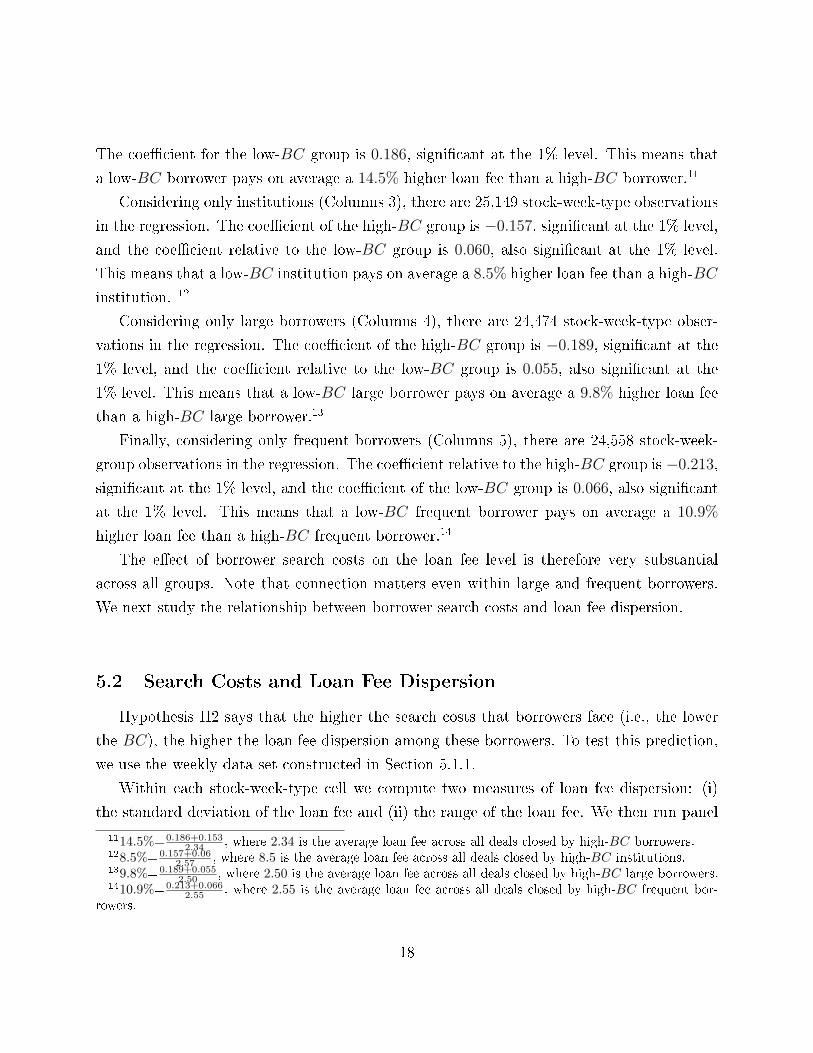
The coe�cient for the low-BC group is 0.186, signi�cant at the 1% level. This means that

a low-BC borrower pays on average a 14.5% higher loan fee than a high-BC borrower.11

Considering only institutions (Columns 3), there are 25,149 stock-week-type observations

in the regression. The coe�cient of the high-BC group is −0.157, signi�cant at the 1% level,

and the coe�cient relative to the low-BC group is 0.060, also signi�cant at the 1% level.

This means that a low-BC institution pays on average a 8.5% higher loan fee than a high-BC

institution. 12

Considering only large borrowers (Columns 4), there are 24,474 stock-week-type obser-

vations in the regression. The coe�cient of the high-BC group is −0.189, signi�cant at the1% level, and the coe�cient relative to the low-BC group is 0.055, also signi�cant at the

1% level. This means that a low-BC large borrower pays on average a 9.8% higher loan fee

than a high-BC large borrower.13

Finally, considering only frequent borrowers (Columns 5), there are 24,558 stock-week-

group observations in the regression. The coe�cient relative to the high-BC group is −0.213,signi�cant at the 1% level, and the coe�cient of the low-BC group is 0.066, also signi�cant

at the 1% level. This means that a low-BC frequent borrower pays on average a 10.9%

higher loan fee than a high-BC frequent borrower.14

The e�ect of borrower search costs on the loan fee level is therefore very substantial

across all groups. Note that connection matters even within large and frequent borrowers.

We next study the relationship between borrower search costs and loan fee dispersion.

5.2 Search Costs and Loan Fee Dispersion

Hypothesis H2 says that the higher the search costs that borrowers face (i.e., the lower

the BC), the higher the loan fee dispersion among these borrowers. To test this prediction,

we use the weekly data set constructed in Section 5.1.1.

Within each stock-week-type cell we compute two measures of loan fee dispersion: (i)

the standard deviation of the loan fee and (ii) the range of the loan fee. We then run panel

1114.5%= 0.186+0.1532.34 , where 2.34 is the average loan fee across all deals closed by high-BC borrowers.

128.5%= 0.157+0.062.57 , where 8.5 is the average loan fee across all deals closed by high-BC institutions.

139.8%= 0.189+0.0552.50 , where 2.50 is the average loan fee across all deals closed by high-BC large borrowers.

1410.9%= 0.213+0.0662.55 , where 2.55 is the average loan fee across all deals closed by high-BC frequent bor-

rowers.

18

regressions of both variables on two dummy variables, High and Low, de�ned as in Section

5.1. As before, we �rst consider all borrowers and then restrict the sample to institutions,

to large borrowers, and to frequent borrowers. All regressions include both stock and week

�xed e�ects. The results are shown in Table 6.


Considering all borrowers (Columns 2 and 3), there are 25,252 stock-week-type observa-

tions in the regression. For the standard deviation measure (Column 2), the coe�cient of

the high-BC type is not signi�cant, while the coe�cient of the low-BC type is 0.246 and

signi�cant at the 1% level. For the range measure (Column 3), the coe�cient of the high-BC

type is −1.264, signi�cant at the 1% level, and the coe�cient of the low-BC type is 1.154,

also signi�cant at the 1% level.

Considering only institutions (Columns 4 and 5), there are 25,097 stock-week-type ob-

servations in the regression. For the standard deviation measure (Column 4), the coe�cient

of the high-BC type is not signi�cant, while the coe�cient of the low-BC type is 0.10, sig-

ni�cant at the 1% level. For the range measure (Column 5), the coe�cient of the high-BC

type is −0.977, signi�cant at the 1% level, and the coe�cient of the low-BC type is 0.612,

also signi�cant at the 1% level.

Considering only large borrowers (Columns 6 and 7), there are 24,474 stock-week-type

observations in the regression. For the standard deviation measure (Column 6), both the

coe�cients for the high-BC and for the low-BC types are not signi�cant. For the range

measure (Column 7), the coe�cient of the high-BC type is −0.919, signi�cant at the 1%

level, and the coe�cient of the low-BC type is 0.156, also signi�cant at the 1% level.

Finally, considering only frequent borrowers (Columns 8 and 9), there are 24,558 stock-

week-type observations in the regression. For the standard deviation measure (Column 8),

the coe�cient of the high-BC type is not signi�cant, while the coe�cient of the low-BC

type is 0.090, signi�cant at the 1% level. For the range measure (Column 9), the coe�cient

of the high-BC type is −1.010, signi�cant at the 1% level, and the coe�cient for the low-BC

type is 0.489, signi�cant at the 1% level.

Using the loan fee standard deviation as the proxy for loan fee dispersion, we conclude

that (i) among low-BC borrowers there is a higher loan fee dispersion than among medium-

19

and high-BC borrowers; (ii) there is no di�erence in loan fee dispersions among medium-

and high-BC borrowers; and (iii) there is no di�erence in dispersion across BC types when

the sample is restricted to large borrowers.

For the unrestricted sample and for the restricted samples for institutions and frequent

borrowers, the di�erence between the loan fee standard deviation among low-BC borrowers

and that of other borrowers is 0.246% (unrestricted), 0.1% (institutions), and 0.09% (fre-

quent borrowers). These numbers are economically signi�cant: the average loan fee standard

deviation is 0.53% (unrestricted), 0.53% (institutions), and 0.54% (frequent borrowers). Con-

sidering for instance the unrestricted sample, this means that the standard deviation among

low-BC borrowers is 46% higher than the standard deviation among high-BC borrowers.15

Using the loan fee range as the proxy for loan fee dispersion, we conclude that (i) there

is a higher loan fee dispersion among low-BC borrowers than among medium-BC borrow-

ers and (ii) there is a higher loan fee dispersion among medium-BC borrowers than among

high-BC borrowers. These results hold for all regressions. The di�erence between the loan

fee range among low-BC borrowers and medium-BC borrowers is 1.154% (unrestricted),

0.612% (institutions), 0.156% (large borrowers), and 0.489% (frequent borrowers). The dif-

ference between the loan fee range among medium-BC borrowers and high-BC borrowers

is 1.264% (unrestricted), 0.977% (institutions), 0.919% (large borrowers), and 1.010% (fre-

quent borrowers). These numbers are economically signi�cant: the average loan fee range

is 1.79% (unrestricted), 1.78% (institutions), 1.79% (large borrowers), and 1.74% (frequent

borrowers). Considering for instance the unrestricted sample, this means that the range

among low-BC borrowers is 135% higher than the range among high-BC borrowers.16

These estimates con�rm that higher borrower search costs yield higher loan fee disper-

sions. As was the case for the average loan fee, the results still hold within borrower type.

In particular, loan fee dispersion increases with search costs even among frequent borrowers.

5.3 Brokerage Fees

In a lending transaction the borrower pays the loan fee plus a brokerage fee. In our

1546% = 0.246%0.53% .

16135% = 1.154%+1.264%1.79% .

20

regressions we considered the loan fee net of this brokerage fee. This is important because

brokerage fee may be directly related to BC, since the broker may charge lower fees from

more important borrowers. Thus, including the brokerage fee in the loan fee would pollute

our analysis.

However, understanding how brokerage fee and search costs relate to each other is im-

portant in itself: high brokerage fees constrain short-sellers by increasing the costs of bor-

rowing.17 Panel A of Table 7 shows the results of the deal-by-deal panel regressions where

the dependent variable is the brokerage fee (p.y., in %) paid by the borrower and the ex-

planatory variable is BC. In Panel B we allow for a nonlinear e�ect of BC on brokerage fees

by grouping borrowers into the high-, medium- and low-BC groups as in Section 5.1. We

compute the average brokerage fee within each stock-week-group cell. We then run panel

regressions of this average brokerage fee within each cell on the two group dummy variables.


The results in Table are consistent with the idea that brokers charge lower fees from

high-BC borrowers. In Panel A, the coe�cients of the BC variable are always negative and

statistically signi�cant at the 1% level across all samples. Panel B shows that that low-

BC borrowers pay higher brokerage fees than medium- and high-BC borrowers. Moreover,

medium-BC borrowers pay higher brokerage fees than high-BC borrowers. Again, the results

hold across all samples.

5.4 Loan Fee Level vs. Loan Fee Dispersion Across Stocks

KRR argue that search costs can be stock-speci�c. For example, it should be relatively

costly to search for small cap and illiquid stocks in the lending market. It is therefore

interesting to compare loan fee dispersion and loan fee level across the stocks in our sample.

If search costs vary at the stock-level then these two variables should be positively related

in the cross-section of stocks.17In our sample, the average brokerage fee is 0.22% p.y. and the median brokerage fee is 0.05% p.y..

Considering only deals closed by frequent borrowers the average is 0.14% p.y. and the median is zero.Considering only deals closed by institutions and large borrowers we get similar numbers, the average is0.15% p.y. and the median is zero.

21

Figure 6 shows a scatter-plot of the stock �xed e�ects estimated in Column 2 of Table

5 and in Column 2 of Table 6. It clearly shows that stocks with higher loan fee dispersion

also have higher loan fee level. This is in line with the results shown in Table VIII of KRR.


5.5 Inside the Top Broker

We have so far have been measuring loan fee dispersion as the standard deviation and

range of the loan fees within stock-day pairs (in Section 3) and within stock-week pairs

(in Section 5.2). In this Section we re�ne these measures by calculating them within a

single broker. Consistent with our previous �ndings, we �nd that (i) di�erent borrowers pay

di�erent loan fees in deals done with the same broker (same stock, same day) and (ii) these

di�erences are related to borrower search costs.

Figure 7 shows all of the 91 brokers in our sample sorted according to the number of

deals closed during the entire period. The biggest broker is responsible for 195,512 loan

deals, twice the number of deals closed by the second-biggest broker (93,966). This volume

of data su�ces to analyze loan fee dispersion inside this single top broker.


We �rst document the existence of loan fee dispersion by computing the standard devia-

tion of loan fees within stock-day pairs using only deals closed inside the top broker. Figure

8 reports the time-series average of the daily loan fee dispersion for each stock. Figure 9

reports the cross-sectional average of the loan fee dispersion for each day. Both �gures show

that even inside the same broker there is signi�cant loan fee dispersion. Moreover, loan fee

dispersion varies considerably both in the cross-section as in the time-series, consistent with

the results in Section 3.

[Figures 8 and 9 about here]

22

We now run regressions of loan fee level and loan fee dispersion on BC, the borrowers'

connection variable.18 We �rst test whether the loan fee level is decreasing in BC in a deal-

by-deal regression. We then test whether loan fee dispersions are higher in groups of low-BC

borrowers.


Table 8 shows the results of the loan fee level regressions. Columns 2 and 3 show the

estimates considering all deals closed inside the top broker (a total of 195,512 observations).

In Column 2 the coe�cient of the BC variable is −0.199, signi�cant at the 1% level. This

means that an increase of 1 percentage point in BC decreases the loan fee level by 0.199

percentage points. Column 3 shows that these results remain the same after controlling for

past volatility and past return.

Columns 4 and 5 show the estimates considering deals from institutions closed inside the

top broker (a total of 25,901 observations). In Column 4, the coe�cient of variable BC is

−0.155 and signi�cant at the 1% level. In Column 5, the results remain after we control for

past volatility and past return.

Columns 6 and 7 show the estimates considering deals from large borrowers closed inside

the top broker (a total of 14,739 observations). In Column 6, the coe�cient of variable BC

is −0.129 and signi�cant at the 1% level. In Column 7, it becomes −0.126.Finally, Columns 8 and 9 show the estimates considering deals from frequent borrowers

closed inside the top broker (a total of 15,335 observations). In Column 8, the coe�cient of

variable BC is −0.123 and signi�cant at the 1% level. In Column 9, it becomes −0.125.Table 9 presents the results for the loan fee dispersion regressions. The regressions are

the same ones shown in Table 6, but with the dependent variables constructed with only

the deals closed inside the top broker. Columns 2 and 3 show the estimates considering

all borrowers (a total of 5,421 stock-week-type observations). For the standard deviation

measure (Column 2), the coe�cient relative to the high-BC type is−0.168, signi�cant at the1% level, and the coe�cient relative to the low-BC type is 0.002, not signi�cant. For the

range measure (Column 3), the coe�cient relative to the high-BC type is −1.355, signi�cant18Although the regressions in this Section include only the deals closed by the top broker, BC is a market-

wide variable, computed using the full sample, as in Section 4.

23

at the 1% level, and the coe�cient relative to the low-connected type is −0.025, but notsigni�cant.


Considering only institutions (Columns 4 and 5), there are 4,021 stock-week-type obser-

vations in the regression. Using the standard deviation measure (Column 4), the coe�cient

of the high-BC type is −0.221, signi�cant at the 1% level, and the coe�cient of the low-BC

type is 0.067, signi�cant at the 5% level. Using the range measure (Column 5), the coe�cient

of the high-BC type is −1.239, signi�cant at the 1% level, and the coe�cient of the low-BC

type is 0.065, but not signi�cant.

Considering only large borrowers (Columns 6 and 7), there are 2,908 stock-week-type

observations. Using the standard deviation measure (Column 6), the coe�cient of the high-

BC type is −0.166, signi�cant at the 1% level, and the coe�cient of the low-BC type is

0.042, not signi�cant. Using the range measure (Column 7), the coe�cient of the high-BC

type is −0.820, signi�cant at the 1% level, and the coe�cient of the low-BC type is −0.017,but not signi�cant.

Finally, considering only frequent borrowers (Columns 8 and 9), there are 3,431 stock-

week-type observations in the regression. For the standard deviation measure (Column 8),

the coe�cient relative to the high-BC type is −0.150, signi�cant at the 1% level, and the

coe�cient of the low-BC type is equal to 0.093, also signi�cant at the 1% level. For the

range measure (Column 9), the coe�cient of the high-BC type is −0.889, signi�cant at the1% level, and the coe�cient of the low-BC type is 0.067, but not signi�cant.

These results show that borrowers with di�erent search costs pay di�erent loan fees in

deals closed even inside the same broker. We take this as a strong evidence in favor of

hypotheses H1 and H2.

5.6 Borrower Connection and Borrower Market Share

Let sharek,s,t be the market share of borrower k with respect to stock s in the 90-day

window previous to day t. Recall that BCk,s,t measures how costly it is for borrower k to

24

search for stock s on day t. This Section discusses the relation between BCk,s,t and sharek,s,t

and shows that sharek,s,t explains neither loan fee levels nor loan fee dispersions. Hence

BCk,s,t encompasses more information than the borrower market share sharek,s,t

The following example illustrates how these two variables di�er. Consider an investor

who during the last 90 days borrowed a large volume of �rm A's stock from a large broker.

During this period the borrower called the broker almost every day searching for stock A,

and closed large loan deals. Assume that today this same borrower calls the broker, but now

searching for stock B. Although the borrower has closed no deals on stock B in the last 90

days, it is likely to be relatively easy for him to search for stock B: he is after all a good

client of the broker, which is therefore highly motivated to do a good job looking for stock B

among its clients. In other words, the borrower's search cost on stock B is not just a function

of his market share in the stock.

Although conceptually di�erent, BCk,s,t and sharek,s,t should be positively related to each

other: both should be high for active borrowers. To con�rm this intuition we run sharek,s,t

on BCk,s,t using our deal-by-deal data set. We �rst use the full sample and then restrict it

to institutions, to large borrowers, and to frequent borrowers. Table 10 displays the results.

The estimates show that the relation between BCk,s,t and sharek,s,t is, as expected, positive

and highly signi�cant.


Although BC and share are positively related, BC should contain more relevant infor-

mation to explain the loan fee level and dispersion, as explained in the example above. We

test this by running deal-by-deal regressions of the loan fee level as the dependent variable,

using both share and BC on the right hand side.


The results in Table 11 are clear. In every regression share does not explain the loan fee

level; by contrast, BC is signi�cant and negatively related to the loan fee levels even after

controlling for share.

25

5.7 A Simpler Borrower-Speci�c Proxy for Search Costs

The computation of the variable BC involves many steps, as presented in Section 4. In

this Section we use a simpler variable as proxy for search costs.

A short-seller calls her broker when she wants to borrow a stock. The broker then tries

to locate the stock, either by searching within its inventory or by contacting lenders. If

the short-seller has an account with a second broker she can access a larger portion of the

lending market. A very simple borrower-speci�c proxy for search costs is thus the number of

accounts the borrower has with di�erent brokers. Although we do not observe this variable

directly, we can estimate it by counting the number of di�erent brokers that intermediated

deals with the borrower in the entire sample. We name this variable accountsk, where k

indexes the borrower. The accountsk variable varies neither in time nor across stocks.

The average number of accounts per borrower is 1.3, the median is 1, and the 95th

percentile is 2. Among institutions, the average is 2.4, the median is 1, and the 95th percentile

is 10. Among large borrowers, the average is 2.9, the median is 1, and the 95th percentile

is 13. Finally, among frequent borrowers, the average is 8.2, the median is 5, and the 95th

percentile is 26.

Table 12 shows the estimates of the deal-by-deal panel regression of loan fee levels on the

two proxies for search costs. Columns 2, 4, 6 and 8 include only accountsk as the search cost

proxy; Columns 3, 5, 7, and 9 include both proxies, accountsk and BCk,s,t. The coe�cient

of accountsk is negative and statistically signi�cant in all regressions � even in those that

also include BCk,s,t. This constitutes additional evidence that borrower-speci�c search costs

drive loan fees.


6 Further Discussion

As shown by many authors, short-selling constraints reduces price e�ciency by excluding

information from price (Asquith et al. (2005), Nagel (2005), Cao et al. (2007), Sa� and

Sigurdsson (2011), Engelberg et al. (2012) and Boehmer and Wu (2013)). As was highlighted

26

by KRR, it follows that the result that search costs a�ect loan fees does have important policy

implications. A regulator could improve price e�ciency in the stock market by reducing

search costs. A natural way to reduce search costs is to reduce the opacity of the lending

market. This could be done for instance via an electronic screen where lending o�ers are seen

by all borrowers. In this Section we present preliminary evidence that a lending electronic

screen reduces both loan fee levels and loan fee dispersion.

In Brazil lending transactions can occur in two ways. Most loan transactions are closed

OTC (in our sample, 90% of the lending volume is OTC). Alternatively, lenders can place

shares for loan directly into an online system where brokers, representing borrowers, can

electronically hit the o�ers.19 Chague et al. (2014) use this feature of the Brazilian market

to identify supply and demand shifts in the lending market and then estimate their e�ects

on stock prices.

The more lending o�ers are placed on the screen, the more information the borrower

has about current market conditions, and so the less opaque the lending market becomes.

We measure opacity by computing for each stock-week pair the proportion screens,t of the

number of shares placed for loan on the electronic screen among the total number of shares

loaned during that week. The numerator of screens,t measures how active the screen is during

the week in terms of the quantity of loan o�ers. The denominator of screens,t measures how

active the whole lending market is during the week. The lower screens,t is, the more opaque

the lending market for stock s in week t is.

The variable screens,t signi�cantly varies both in the cross-section and in the time-series.

However, the reasons behind these variations are not clear. In what follows we directly

relate loan fee level and dispersion to screens,t. Since the variation in screens,t might not

be exogenous, we acknowledge that this exercise provides only preliminary evidence on the

e�ect that an active lending platform could have on loan fee levels.

We regress (i) the standard deviation of loan fees within each stock-week pair on the

screens,t variable, (ii) the range of loan fees within each stock-week pair on the screens,t

variable, and (iii) the average loan fee within each stock-week pair on the screens,t variable.

We standardize the screens,t variable within each �rm in order to purge it of stock-speci�c

characteristics and to allow a better interpretation of the results. As usual, we �rst consider

all deals (from all types of borrowers) and then we restrict the sample to deals from institu-

19Only brokers have access to this electronic screen.

27

tions, deals from large borrowers, and deals from frequent borrowers. Table 13 presents the

results.


Considering all deals, we �nd that during weeks when the number of lending o�ers on the

screen is one standard deviation higher than the average the standard deviation of loan fees

across deals is 0.057% lower, the range of loan fees is 0.441% lower, and the average loan fee

is 0.193% lower, all signi�cant at the 1% level. Considering deals only from institutions, the

corresponding coe�cients are 0.049% for the standard deviation, 0.394% for the range, and

0.187% for the average loan fee, all signi�cant at the 1% level. Considering deals only from

large borrowers, the coe�cients are 0.054% for the standard deviation, 0.365% for the range,

and 0.190% for the average loan fee, all signi�cant at the 1% level. Finally, considering deals

only from frequent borrowers, the coe�cients are 0.049% for the standard deviation, 0.371%

for the range, and 0.187% for the average loan fee, all signi�cant at the 1% level.

These estimates indicate that an active electronic screen in the lending market can reduce

both loan fee levels and loan fee dispersion. Regulators should therefore encourage the use of

such platforms to reduce opacity and hence search costs in the lending market, which would

increase price e�ciency in the overall stock market.

7 Concluding Remarks

This study yields empirical evidence regarding the e�ects of borrower-speci�c search

costs on equity loan fees. We introduce a measure of search cost that is based on borrowers'

connections and thus views the lending market as a relationship-based market. The degree of

the borrower connectedness is calculated using a unique data set that comprises all loan deals

in the Brazilian market from January 2008 to July 2011. For each deal we have information

on the loan quantity, the loan fee, the borrower type, the borrower ID, the broker ID, and

the lender ID.

Our empirical results con�rm DGP's prediction that higher search costs result in higher

loan fees. These results are robust to di�erent speci�cations of search costs and still hold

28

when the sample is restricted to institutions, to large borrowers, and to frequent borrow-

ers. Our results extend the �ndings by KRR that document stock-speci�c search costs as

important determinants of loan fees.

Since higher loan fees and loan fee dispersion increase the costs and the risks of short-

selling, an important policy implication is that a reduction of search costs in the lending

market is very desirable. As KRR points out, this can be directly achieved by implementing

a centralized trade platform. We contribute to this discussion by documenting the e�ect

that the proportion of lending o�ers placed on the Brazilian electronic lending platform has

on loan fees.

29

References

Allen, Franklin, and Ana Babus, 2009, Networks in �nance, in The Network Challenge:

Strategy, Pro�t, and Risk in an Interlinked World , chapter 21 (Pearson Prentice Hall).

Ang, Andrew, Assaf A. Shtauber, and Paul C. Tetlock, 2013, Asset Pricing in the Dark: The

Cross-Section of OTC Stocks, Review of Financial Studies 26, 2985�3028.

Asquith, Paul, Parag A. Pathak, and Jay R. Ritter, 2005, Short interest, institutional own-

ership, and stock returns, Journal of Financial Economics 78, 243 � 276.

Astorino, Eduardo, Fernando Chague, Bruno Cara Giovannetti, and Marcos E. Silva, 2015,

Variance Premium and Implied Volatility in a Low-Liquidity Option Market, SSRN Schol-

arly Paper ID 2592650, Social Science Research Network, Rochester, NY.

Blocher, Jesse, Adam V. Reed, and Edward D. Van Wesep, 2013, Connecting two mar-

kets: An equilibrium framework for shorts, longs, and stock loans, Journal of Financial

Economics 108, 302�322.

Boehmer, Ekkehart, and Juan (Julie) Wu, 2013, Short Selling and the Price Discovery Pro-

cess, Review of Financial Studies 26, 287�322.

Cao, Bing, Dan S. Dhaliwal, Adam C. Kolasinski, and Adam V. Reed, 2007, Bears and

Numbers: Investigating How Short Sellers Exploit and A�ect Earnings-Based Pricing

Anomalies, SSRN Scholarly Paper ID 748506, Social Science Research Network, Rochester,

NY.

Chague, Fernando, Rodrigo De-Losso, Alan De Genaro, and Bruno Giovannetti, 2014, Short-

sellers: Informed but restricted, Journal of International Money and Finance 47, 56�70.

Chang, Eric, Joseph W. Cheng, and Yingchui Yu, 2007, Short-Sales Constraints and Price

Discovery: Evidence from the Hong Kong Market, The Journal of Finance 62, 2097�2121.

Danielsen, Bartley R., and Sorin M. Sorescu, 2001, Why Do Option Introductions Depress

Stock Prices? A Study of Diminishing Short Sale Constraints, The Journal of Financial

and Quantitative Analysis 36, 451�484.

30

D'Avolio, Gene, 2002, The market for borrowing stock, Journal of Financial Economics 66,

271 � 306.

Du�e, Darrell, Nicolae Garleanu, and Lasse Heje Pedersen, 2002, Securities lending, short-

ing, and pricing, Journal of Financial Economics 66, 307 � 339.

Du�e, Darrell, Nicolae Garleanu, and Lasse Heje Pedersen, 2005, Over-the-Counter Markets,

Econometrica 73, 1815�1847.

Du�e, Darrell, Nicolae Garleanu, and Lasse Heje Pedersen, 2007, Valuation in Over-the-

Counter Markets, Review of Financial Studies 20, 1865�1900.

Du�e, Darrell, Gaston Giroux, and Gustavo Manso, 2010, Information Percolation, Ameri-

can Economic Journal: Microeconomics 2, 100�111.

Du�e, Darrell, Semyon Malamud, and Gustavo Manso, 2009, Information Percolation With

Equilibrium Search Dynamics, Econometrica 77, 1513�1574.

Du�e, Darrell, and Gustavo Manso, 2007, Information Percolation in Large Markets, The

American Economic Review 97, 203�209.

Engelberg, Joseph, Adam V. Reed, and Matthew Ringgenberg, 2013, Short Selling Risk,

SSRN Scholarly Paper ID 2312625, Social Science Research Network, Rochester, NY.

Engelberg, Joseph E., Adam V. Reed, and Matthew C. Ringgenberg, 2012, How are shorts in-

formed?: Short sellers, news, and information processing, Journal of Financial Economics

105, 260�278.

Eraker, Bjorn, and Mark Ready, 2015, Do investors overpay for stocks with lottery-like

payo�s? An examination of the returns of OTC stocks, Journal of Financial Economics

115, 486�504.

Jones, Charles M., and Owen A. Lamont, 2002, Short-sale constraints and stock returns,

Journal of Financial Economics 66, 207 � 239.

Kolasinski, Adam C., Adam V. Reed, and Matthew C. Ringgenberg, 2013, A Multiple Lender

Approach to Understanding Supply and Search in the Equity Lending Market, The Journal

of Finance 68, 559�595.

31

Nagel, Stefan, 2005, Short sales, institutional investors and the cross-section of stock returns,

Journal of Financial Economics 78, 277 � 309.

Newman, M., 2010, Networks: An Introduction (OUP Oxford).

Prado, Melissa Porras, 2015, Future Lending Income and Security Value, Journal of Finan-

cial and Quantitative Analysis .

Reed, Adam V., 2013, Short Selling, Annual Review of Financial Economics 5, 245�258.

Sa�, Pedro A. C., and Kari Sigurdsson, 2011, Price E�ciency and Short Selling, Review of

Financial Studies 24, 821�852.

Stambaugh, Robert F., Jianfeng Yu, and Yu Yuan, 2012, The short of it: Investor sentiment

and anomalies, Journal of Financial Economics 104, 288�302.

Zhu, Haoxiang, 2012, Finding a Good Price in Opaque Over-the-Counter Markets, Review

of Financial Studies 25, 1255�1285.

32

Tables and Figures

Figure 1: Loan Fee Dispersion - Four Stocks

This Figure shows the loan fee dispersion for the 4 stocks with the largest number of loan deals in our sample,

namely, VALE5 (131,441 deals), PETR4 (107,263 deals), GGBR4 (78,916 deals) and BBDC4 (70,311). Loan

fee dispersion is calculated as the standard deviation of the annualized loan fee in percentage points of all

deals for the same stock on the same day. Each point in the Figure is the loan fee dispersion of a day from

January 2008 to July 2011.

33

Figure 2: Loan Fee Dispersion in the Cross-Section

This Figure shows the time-series average of the loan fee dispersion for each stock in our sample. For each

one of the 55 stocks in our sample we compute the average of its daily loan fee dispersion from January

2008 to July 2011. Loan fee dispersion is calculated as the standard deviation of the annualized loan fee in

percentage points of all deals for the same stock on the same day. The 55 stocks are alphabetically ordered

on the x-axis.

34

Figure 3: Loan Fee Dispersion in the Time-series

This Figure shows the cross-sectional average of the loan fee dispersion for each day in our sample. For each

trading day from January 2008 to July 2011, we compute the average of the loan fee dispersion across the

55 stocks in our sample. Loan fee dispersion is calculated as the standard deviation of the annualized loan

fee in percentage points of all deals for the same stock on the same day.

35

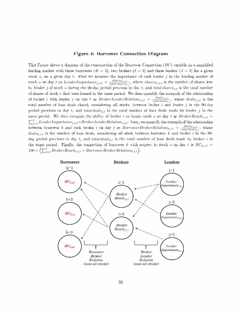
Figure 4: Borrower Connection Diagram

This Figure shows a diagram of the construction of the Borrower Connection (BC) variable in a simpli�ed

lending market with three borrowers (K = 3), two brokers (I = 2) and three lenders (J = 3) for a given

stock s, on a given day t. First we measure the importance of each lender j in the lending market of

stock s on day t as LenderImportancej,s,t =sharesj,s,t

total sharess,t, where sharesj,s,t is the number of shares lent

by lender j of stock s during the 90-day period previous to day t, and total sharess,t is the total number

of shares of stock s that were loaned in the same period. We then quantify the strength of the relationship

of broker i with lender j on day t as BrokerLenderRelationi,j,t =dealsi,j,t

total dealsj,t, where dealsi,j,t is the

total number of loan deals closed, considering all stocks, between broker i and lender j in the 90-day

period previous to day t, and total dealsj,t is the total number of loan deals made by lender j in the

same period. We then compute the ability of broker i to locate stock s on day t as BrokerReachi,s,t =∑Jj=1 LenderImportancej,s,t×BrokerLenderRelationi,j,t. Next, we quantify the strength of the relationship

between borrower k and each broker i on day t as BorrowerBrokerRelationk,i,t =dealsk,i,t

total dealsi,t, where

dealsk,i,t is the number of loan deals, considering all stock, between borrower k and broker i in the 90-

day period previous to day t, and total dealsi,t is the total number of loan deals made by broker i in

the same period. Finally, the connection of borrower k with respect to stock s on day t is BCk,s,t =

100×(∑I

i=1 BrokerReachi,s,t ×BorrowerBrokerRelationk,i,t

).

36

Figure 5: Borrower Connection

This Figure shows the Borrower Connection (BC) variable of four arbitrary frequent borrowers on four of

the most liquid stocks in the lending market: Petrobras PN (PETR4), Bradesco PN (BBDC4), Gerdau PN

(GGBR4) and Vale do Rio Doce PN (VALE5). The calculation of the variable BC is described in Section

4. BC is a time-varying (at the daily frequency) and stock-speci�c variable which it is decreasing in the

borrower's search costs. A high value here means that the borrower has strong relationships with brokers

which in turn have strong relationships with important lenders of the stock. The sample period is from July

of 2008 to July 2011, and the frequency is daily.

0.0

05.0

1.0

15

0.2

.4.6

0.1

.2.3

0.0

5.1

Frequent Borrower #1 Frequent Borrower #2

Frequent Borrower #3 Frequent Borrower #4

BBDC4 GGBR4PETR4 VALE5

Bor

row

er C

onne

ctio

n (B

C)

Day

37

Figure 6: Level Fixed E�ect vs. Dispersion Fixed E�ect

This Figure shows the scatter-plot between the level �xed e�ect and the dispersion �xed e�ect of each one

of the 55 stocks in our sample. The level �xed e�ect is the stock �xed e�ect estimated in Table 5. The

dispersion �xed e�ect is the stock �xed e�ect estimated in Table 6.

−20

24

6

Leve

l Fix

ed−E

ffect

s

−.5 0 .5 1 1.5

Dispersion Fixed−Effects

38

Figure 7: Number of Loan Deals by Brokers

This Figure shows the number of lending deals intermediated by each broker during January 2008 and July

2011. The 91 brokers are sorted on the x-axis according to the total number of deals.

Top Broker

050

000

1000

0015

0000

2000

00N

umbe

r of

dea

ls

0 20 40 60 80 100Brokers

39

Figure 8: Inside the Top Broker: Loan Fee Dispersion in the Cross-section

This Figure shows the time-series average of the loan fee dispersion inside the top broker for each stock

in our sample. For each one of the 55 stocks in our sample, we compute the average of its daily loan fee

dispersion from January 2008 to July 2011. Loan fee dispersion is calculated as the standard deviation of

the annualized loan fee in percentage points of all deals intermediated by the top broker for the same stock

on the same day. The 55 stocks are alphabetically ordered on the x-axis. The top broker is the broker with

the highest number of closed deals in the entire sample.

40

Figure 9: Inside the Top Broker: Loan Fee Dispersion in the Time-series

This Figure shows the cross-sectional average of the loan fee dispersion inside the top broker for each day in

our sample. For each trading day from January 2008 to July 2011, we compute the average of the loan fee

dispersion across the 55 stocks in our sample. Loan fee dispersion is calculated as the standard deviation of

the annualized loan fee in percentage points of all deals intermediated by the top broker for the same stock

on the same day. The top broker is the broker with the highest number of deals closed in the entire sample.

41

Table 1: Number of Borrowers and Lenders by Year

This Table shows the number of di�erent borrowers and lenders in the lending market per year. The data

set identi�es each investor with a unique ID. An investor who closed both a borrowing and a lending deal in

the same year is included in both columns. The last line considers only the �rst 7 months of 2011.

Year # of Borrowers # of Lenders2008 17,435 3,4712009 22,166 3,4162010 24,809 6,785

2011 (Jan-Jul) 16,515 8,103

42

Table 2: Descriptive Statistics by Stock

This Table reports, stock by stock, the stock ticker, the average Loan Fee Dispersion (LFD), the standard

deviation of the LFD, the daily average number of loan deals, and the average loan fee (% per year). We

measure LFD as the standard deviation of the annualized loan fee of all deals for the same stock on a given

day.

TickerLoan Fee Dispersion Loan Deals

Avg. Std. Dev. Per Day Fee (in %)

AMBV4 0.32 0.58 58 0.65

BBAS3 0.61 1.24 80 1.04

BBDC4 0.43 0.43 113 0.54

BRAP4 0.25 0.33 26 0.74

BRKM5 0.55 0.45 49 1.88

BRML3 0.62 0.77 27 5.18

BRTO4 0.88 2.02 24 2.36

BTOW3 1.77 1.88 33 5.16

CCRO3 0.90 1.17 31 3.33

CESP6 0.91 0.80 25 1.72

CMIG4 0.69 0.58 66 2.07

CPFE3 0.86 0.61 48 4.82

CPLE6 0.60 0.49 29 2.20

CRUZ3 0.42 0.39 61 2.12

CSAN3 1.26 1.73 33 5.34

CSMG3 0.62 1.19 8 3.49

CSNA3 0.36 0.38 91 0.86

CYRE3 1.32 1.54 56 6.03

ELET3 0.62 0.84 22 1.90

ELET6 0.78 1.20 58 4.32

EMBR3 0.65 0.89 33 2.46

ENBR3 0.71 1.11 19 4.41

FFTL4 0.59 0.76 15 1.80

GFSA3 1.29 1.26 45 6.17

GGBR4 0.71 0.88 118 2.19

GOAU4 0.29 0.66 26 0.52

GOLL4 1.46 1.20 31 4.87

ITSA4 0.26 0.38 55 0.41

JBSS3 1.97 1.83 48 8.20

KLBN4 0.53 0.88 54 2.67

LAME4 0.80 0.76 66 3.28

LIGT3 0.99 1.32 42 4.64

LREN3 1.28 0.89 51 6.15

MRVE3 1.40 1.93 56 6.92

NATU3 1.06 0.97 67 6.25

43

(continues from previous page).

TickerLoan Fee Dispersion Loan Deals

Avg. Std. Dev. Per Day Fee (in %)

PETR3 0.36 0.92 62 0.70

PETR4 0.62 0.95 154 0.77

RDCD3 1.49 1.62 71 7.20

RENT3 0.35 0.49 28 3.58

RSID3 1.13 1.40 44 4.87

SBSP3 0.83 1.24 22 2.50

SUZB5 0.50 0.49 22 2.38

TAMM4 1.38 1.28 29 3.57

TBLE3 0.40 0.38 26 2.13

TCSL4 1.11 1.21 44 5.24

TMAR5 1.14 1.32 19 4.38

TNLP3 0.56 0.73 12 2.25

TNLP4 0.87 0.73 59 3.42

TRPL4 0.44 0.50 19 1.81

UGPA4 0.33 0.88 25 1.05

USIM3 1.40 1.67 32 5.13

USIM5 0.44 0.37 92 1.26

VALE3 0.40 0.41 77 0.64

VALE5 0.42 0.33 169 0.47

WEGE3 0.76 0.80 23 3.76

44

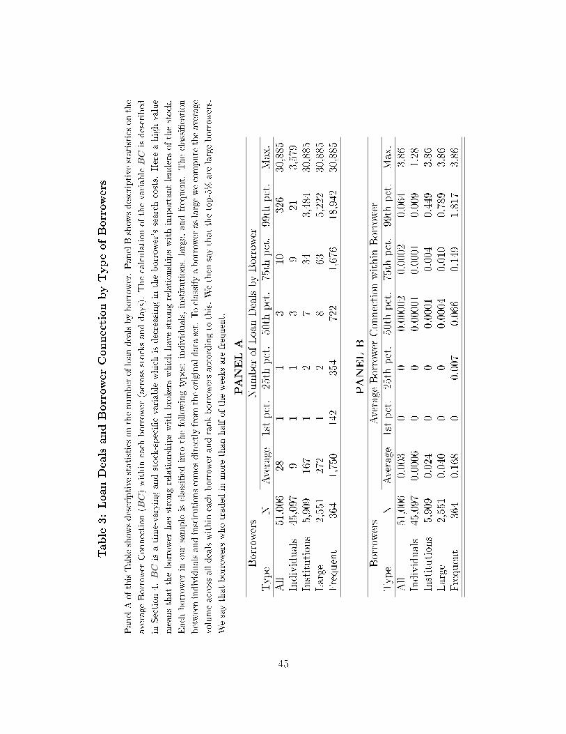
Table3:LoanDealsandBorrowerConnectionbyTypeofBorrowers

PanelAofthisTableshow

sdescriptivestatisticsonthenumberofloandealsbyborrow

er.PanelBshow

sdescriptivestatisticsonthe

averageBorrow

erConnection(B

C)within

each

borrow

er(across

stocksanddays).Thecalculationofthevariable

BC

isdescribed

inSection4.BC

isatime-varyingandstock-speci�cvariablewhichisdecreasingin

theborrow

er'ssearchcosts.

Hereahighvalue

meansthattheborrow

erhasstrongrelationshipswithbrokerswhichhavestrongrelationshipswithimportantlendersofthestock.

Each

borrow

erin

oursampleisclassi�ed

into

thefollow

ingtypes:individuals,institutions,large,

andfrequent.

Theclassi�cation

betweenindividualsandinstitutionscomesdirectlyfromtheoriginaldata

set.Toclassifyaborrow

eraslargewecomputetheaverage

volumeacrossalldealswithin

each

borrow

erandrankborrow

ersaccordingto

this.Wethen

saythatthetop-5%

are

largeborrow

ers.

Wesaythatborrow

erswhotraded

inmore

thanhalfoftheweeksare

frequent.

PANELA

Borrowers

Number

ofLoanDealsbyBorrower

Type

NAverage

1stpct.

25th

pct.

50th

pct.

75th

pct.

99th

pct.

Max.

All

51,006

281

13

10326

30,885

Individuals

45,097

91

13

921

3,579

Institutions

5,909

167

12

734

3,484

30,885

Large

2,551

272

12

863

5,222

30,885

Frequent

364

1,750

142

354

722

1,676

18,942

30,885

PANELB

Borrowers

Average

Borrower

Connection

within

Borrower

Type

NAverage

1stpct.

25th

pct.

50th

pct.

75th

pct.

99th

pct.

Max.

All

51,006

0.003

00

0.00002

0.0002

0.064

3.86

Individuals

45,097

0.0006

00

0.00001

0.0001

0.009

1.28

Institutions

5,909

0.024

00

0.0001

0.004

0.449

3.86

Large

2,551

0.040

00

0.0004

0.010

0.789

3.86

Frequent

364

0.168

00.007

0.066

0.149

1.817

3.86

45

Table4:LoanFeeLevelasaFunctionofBorrowerConnection

ThisTableshow

stheestimatesofdeal-by-dealpanelregressionswiththeloanfeeasthedependentvariable.Columns2,4,6and8

haveBorrow

erConnection(B

C)asthemain

explanatory

variableandPast

Volatility

andPast

Return

ascontrols.Thecalculation

ofthevariable

BC

isdescribed

inSection4.

BC

isatime-varying(atthedailyfrequency)andstock-speci�cvariable

whichis

decreasingin

theborrow

er'ssearchcosts.

Ahighvalueheremeansthattheborrow

erhasstrongrelationshipswithbrokerswhich

havestrongrelationshipswithimportantlendersofthestock.Past

Volatility

isthestandard

deviationofstock

returnsonthepast

5days.

Past

Return

isthestock

return

onthelast

5days.

Columns3,5,7,and9includeBroker

Reach

asanadditionalcontrol,

whichmeasureshow

well-connectisthebroker

(thatinterm

ediatesthedeal)withlendersofthespeci�cstock.Columns2and4

show

theestimatesconsideringalldealsin

oursample.Theother

Columnsshow

theestimatesfortherestricted

samplesaccording

totheborrow

ertype.

Each

borrow

erin


into

thefollow

ingtypes:individuals,institutions,large,andfrequent.

Theclassi�cationbetweenindividualsandinstitutionscomes

directlyfrom

theoriginaldata

set.

Toclassifyaborrow

eraslargewe

computetheaveragevolumeacrossalldealswithineach

borrow

erandrankborrow

ersaccordingto

this.Wethen

saythatthetop-5%

arelargeborrow

ers.Wesaythatborrow

erswhotraded

inmorethanhalfoftheweeksarefrequent.Allregressionsincludestock-week

�xed

e�ects,i.e.,dummyvariablesforeach

pairstock-week.Standard

errorsare

presentedin

parentheses

andare

clustered

bystock.

***,**,*indicate

signi�cance

atthe1%,5%

and10%

level,respectively.

Dealsfrom

Dealsfrom

large

Dealsfrom

frequent

AllDeals

institutions

borrowers

borrowers

Borrower

Connection

-0.088***

-0.081***

-0.058***

-0.055***

-0.055***

-0.053***

-0.057***

-0.054***

(0.013)

(0.012)

(0.010)

(0.010)

(0.011)

(0.011)

(0.011)

(0.011)

BrokerReach

-0.008***

-0.004***

-0.003**

-0.004**

(0.002)

(0.002)

(0.001)

(0.002)

PastVolatility

0.041**

0.040**

0.047**

0.047**

0.053**

0.053**

0.051**

0.051**

(0.019)

(0.019)

(0.022)

(0.022)

(0.023)

(0.023)

(0.021)

(0.021)

PastReturn

0.001

0.001

-0.001

-0.001

-0.001

-0.001

-0.002

-0.002

(0.001)

(0.001)

(0.002)

(0.002)

(0.002)

(0.002)

(0.002)

(0.002)

Stock-W

eekFixed

E�ects

Yes

Yes

Yes

Yes

Yes

Yes

Yes

Yes

N1,251,801

1,251,801

912,579

912,579

641,744

641,744

605,916

605,916

R2−adj

0.83

0.83

0.84

0.84

0.84

0.84

0.85

0.85

46

Table 5: Loan Fee Level for High-, Medium- and Low-connected Borrowers

This Table presents estimates of nonlinear e�ects of BC on the loan fee. Within each stock-week pair, we

rank deals with respect to the borrowers' BC and classify them into three groups: low-BC group if BC

falls below the 50%-percentile, medium-BC group if it falls between the 50%- and the 90%-percentile, and

high-BC group if it falls above the 90%-percentile. For each stock-week-group cell we compute the average

loan fee across all deals. We then run panel regressions of this average loan fee on two dummy variables,

High and Low. High takes value one if the cell refers to the high-BC group and zero otherwise. Low

takes value one if the cell refers to the low-BC and zero otherwise. BC is a time-varying and stock-speci�c

variable which is decreasing in the borrower's search costs. The calculation of the variable BC is described

in Section 4. Column 2 in the Table shows the estimates considering all deals in our sample. Columns 3, 4,

and 5 consider deals from samples restricted according to borrowers type: institutional, large and frequent.

Classi�cation between individuals and institutions comes directly from the original data set. To classify a

borrower as large we compute the average volume across all deals within each borrower and rank borrowers

according to this. We then say that the top-5% are large borrowers. We say that borrowers who traded

in more than half of the weeks are frequent. All regressions include stock and week �xed e�ects. Standard

errors are presented in parentheses and are clustered by stock. ***, **, * indicate signi�cance at the 1%, 5%

and 10% level, respectively.

All Borrowers Institutions Large FrequentHigh -0.153*** -0.157*** -0.189*** -0.213***

(0.028) (0.029) (0.037) (0.038)Low 0.186*** 0.060*** 0.055** 0.066***

(0.026) (0.020) (0.023) (0.024)Stock Fixed E�ects Yes Yes Yes YesWeek Fixed E�ects Yes Yes Yes Yes

N 25,323 25,149 24,474 24,558R2 − adj 0.53 0.52 0.51 0.51

47

Table6:LoanFeeDispersionforHigh-,Medium-andLow-connectedBorrowers

ThisTablepresentsestimatesofthee�ectofBorrow

erConnection(B

C)ontheloanfeedispersion.Within

each

stock-weekpairwe

rankdealswithrespectto

theborrow

ers'BCandclassifythem

into

threegroups:low-B

CgroupifBCfallsbelow

the50%-percentile,

medium-B

Cgroupifitfallsbetweenthe50%-andthe90%-percentile,andhigh-B

Cgroupifitfallsabovethe90%-percentile.For

each

stock-week-groupcell,wecompute

twomeasuresofloanfeedispersion:thestandard

deviationandtherangeofloanfees

across

alldeals.Wethen

runpanelregressionsofthesedispersionmeasuresontwodummyvariables,HighandLow

.Hightakes

valueone

ifthecellrefers

tothehigh-B

Cgroupandzero

otherwise.

Low

takes

valueoneifthecellrefers

tothelow-B

Candzero

otherwise.

BCisatime-varyingandstock-speci�cvariablewhichitisdecreasingin

theborrow

er'ssearchcosts.Thecalculationofthevariable

BC

isdescribed

inSection4.Columns2and3in

theTable

show


oursample.Theother

columnsconsider

dealsfrom

samplesrestricted

accordingto

borrow

erstype:

institutional,large,andfrequent.Classi�cationbetween

individualsandinstitutionscomes

directlyfromtheoriginaldata


eraslarge,wecomputetheaveragevolume

across

alldealswithin

each

borrow

erandrankborrow

ersaccordingto

this.Wethen

saythatthetop-5%

are

largeborrow

ers.

We

saythatborrow

erswhotraded

inmore


frequent.

Allregressionsincludestock

andweek�xed

e�ects.

Standard

errorsare

presentedin

parentheses

andare

clustered

bystock.***,**,*indicate

signi�cance

atthe1%,5%

and10%

level,

respectively.

AllBorrowers

Institutions

Large

Frequent

Std.Dev.

Range

Std.Dev.

Range

Std.Dev.

Range

Std.Dev.

Range

High

-0.016

-1.264***

0.027

-0.977***

0.043

-0.919***

0.018

-1.010***

(0.025)

(0.096)

(0.023)

(0.079)

(0.027)

(0.074)

(0.029)

(0.085)

Low

0.246***

1.154***

0.100***

0.612***

0.012

0.156***

0.090***

0.489***

(0.021)

(0.101)

(0.015)

(0.065)

(0.016)

(0.055)

(0.017)

(0.061)

Stock

Fixed

E�ect

Yes

Yes

Yes

Yes

Yes

Yes

Yes

Yes

WeekFixed

E�ect

Yes

Yes

Yes

Yes

Yes

Yes

Yes

Yes

N25,252

25,252

25,097

25,097

24,474

24,474

24,558

24,558

R2−adj

0.25

0.33

0.22

0.29

0.21

0.25

0.21

0.28

48

Table 7: Brokerage Fee and Borrowers Connection

Panel A of this Table shows the estimates of deal-by-deal panel regressions of brokerage fee on Borrower

Connection (BC). Brokerage fee is the fee in % p.y. paid by borrower in the loan deal. BC is a time-varying

and stock-speci�c variable which is decreasing in the borrower's search costs. The calculation of the variable

BC is described in Section 4. Panel B presents estimates of nonlinear e�ects of BC on brokerage fee. Within

each stock-week pair we rank deals with respect to the borrowers BC and classify them into three groups:

low-BC group if BC falls below the 50%-percentile, medium-BC group if it falls between the 50%- and the

90%-percentile, and high-BC group if it falls above the 90%-percentile. For each stock-week-group cell we

compute the average brokerage fee across all deals. We then run panel regressions of this average brokerage

fee on two dummy variables, High and Low. High takes value one if the cell refers to the high-BC group

and zero otherwise. Low takes value one if the cell refers to the low-BC and zero otherwise. Column 2 of

both Panels shows the estimates considering all deals in our sample. Columns 3, 4, and 5 consider deals from

samples restricted according to borrowers type: institutional, large, and frequent. Classi�cation between

individuals and institutions comes directly from the original data set. To classify a borrower as large, we

do the following. We compute the average volume across all deals within each borrower and rank borrowers

according to this. We then say that the top-5% are large borrowers. We say that borrowers that traded

in more than half of the weeks are frequent. All regressions include stock and time �xed e�ects. Standard

errors are presented in parentheses and are clustered by stock. ***, **, * indicate signi�cance at the 1%, 5%

and 10% level, respectively.

PANEL A

Deals from Deals from large Deals from frequentAll deals institutions borrowers borrowers

Borrower Connection -0.042*** -0.013*** -0.010*** -0.012***(0.005) (0.002) (0.002) (0.002)

Stock-Week Fixed E�ect Yes Yes Yes YesN 1,251,801 912,579 641,744 605,916

R2 − adj 0.024 0.022 0.022 0.026

PANEL B


High -0.034*** -0.017*** -0.018*** -0.023***(0.005) (0.005) (0.005) (0.005)

Low 0.158*** 0.050*** 0.030*** 0.052***(0.006) (0.005) (0.004) (0.005)

Stock Fixed E�ect Yes Yes Yes YesWeek Fixed E�ect Yes Yes Yes Yes

N 25,258 25,103 24,479 24,562R2 − adj 0.187 0.084 0.078 0.080

49

Table8:InsidetheTopBroker:LoanFeeLevelasaFunctionofBorrowerConnection

ThisTableshow

stheestimatesofdeal-by-dealpanelregressionswiththeloanfeeasthedependentvariable.Allregressionsconsider

onlydealsinterm

ediatedbythetopbroker.Thetopbrokeristhebrokerwiththehighestnumberofdealsclosedintheentiresample.

Columns2,4,6and8haveBorrow

erConnection(B

C)astheexplanatory

variable.Thecalculationofthevariable

BCisdescribed

inSection4.BCisatime-varying(atthedailyfrequency)andstock-speci�cvariable,anditisdecreasingin

thesearchcostsofthe

borrow

er.Ahighvalueofthisvariablemeansthattheborrow

erhasstrongrelationshipswithbrokerswithstrongrelationshipswith

importantlendersofthestock.Columns3,5,7,and9includePast

Volatility

andPast

Return

ascontrolvariables.

Past

Volatility

isthestandard

deviationofstock

returnsonthepast

5days.

Past

Return

isthestock

return

onthelast

5days.

Columns2and4

show


oursample.Theother

Columnsshow


samplesaccording

totheborrow

ertype.

Each

borrow

erin


into

thefollow

ingtypes:individuals,institutions,large,andfrequent.


directlyfrom

theoriginaldata

set.

Toclassifyaborrow

eraslarge,we

dothefollow

ing.Wecompute

theaveragevolumeacrossalldealswithin

each

borrow

erandrankborrow

ersaccordingto

this.Then,

wesaythatthetop-5%

are

largeborrow

ers.

Finally,wesaythatborrow

ersthattraded

inmore


frequent.

Allregressionsincludestock

andday

�xed

e�ects.Standard

errorsare

presentedin

parentheses

andare

clustered

bystock.***,**,

*indicate

signi�cance

atthe1%,5%

and10%

level,respectively.

AllBorrowers

Institutions

Large

Frequent

Borrower

Connection

-0.199***

-0.195***

-0.155***

-0.151***

-0.129***

-0.126***

-0.123***

-0.125***

(0.067)

(0.069)

(0.049)

(0.048)

(0.048)

(0.046)

(0.043)

(0.042)

PastVolatility

0.144**

0.170*

0.200**

0.113**

(0.065)

(0.083)

(0.088)

(0.051)

PastReturn

-0.002

0.010

0.012

-0.001

(0.005)

(0.007)

(0.009)

(0.009)

Stock

Fixed

E�ects

Yes

Yes

Yes

Yes

Yes

Yes

Yes

Yes

Day

Fixed

E�ects

Yes

Yes

Yes

Yes

Yes

Yes

Yes

Yes

N195,512

195,512

25,901

25,901

14,739

14,739

15,335

15,335

R2−adj

0.59

0.59

0.57

0.58

0.58

0.58

0.61

0.61

50

Table

9:InsidetheTopBroker:LoanFeeDispersionforHigh-,

Medium-andLow-connected

Borrowers

ThisTablepresentsestimatesofthee�ectofBorrow

erConnection(B

C)ontheloanfeedispersion.Allregressionsconsideronlydeals

interm

ediatedbythetopbroker.Thetopbroker

isthebroker

withthehighestnumber

ofdealsclosedin

theentire

sample.Within

each

stock-weekpairwerankdealswithrespectto

theborrow

ersBC

andclassifythem

into

threegroups:

low-B

CgroupifBC

fallsbelow

the50%-percentile,medium-B

Cgroupifitfallsbetweenthe50%-andthe90%-percentile,andhigh-B

Cgroupifitfalls

abovethe90%-percentile.Foreach

stock-week-groupcellwecompute

twomeasuresofloanfeedispersion:thestandard

deviation

andtherangeofloanfees

acrossalldeals.Wethen

runpanelregressionsofthesedispersionmeasuresontwodummyvariables,High

andLow

.Hightakes


tothehigh-B

Cgroupandzero

otherwise.

Low

takes


tothelow-B

Candzero

otherwise.

BC

isatime-varyingandstock-speci�cvariablewhichisdecreasingin

thesearchcostsofthe

borrow

er.Thecalculationofthevariable

BCisdescribed

inSection4.Columns2and3in

theTableshow

theestimatesconsidering

alldealsin

oursample.Theother

columnsconsider

dealsfrom

samplesrestricted

accordingto

borrow

erstype:

institutional,large,

andfrequent.

Classi�cationbetweenindividualsandinstitutionscomes

directlyfrom

theoriginaldata

set.

Toclassifyaborrow

er

aslarge,wecompute

theaveragevolumeacross

alldealswithin

each

borrow

erandrankborrow

ersaccordingto

this.Wethen

say

thatthetop-5%

are

largeborrow

ers.Wesaythatborrow

ersthattraded

inmore


frequent.Allregressions

includestock

andweek�xed

e�ects.Standard

errors

are

presentedin

parentheses

andare

clustered


signi�cance

atthe1%,5%

and10%

level,respectively.

AllBorrowers

Institutions

Large

Frequent

Std.Dev.

Range

Std.Dev.

Range

Std.Dev.

Range

Std.Dev.

Range

High

-0.168***

-1.355***

-0.221***

-1.239***

-0166***

-0.820***

-0.150***

-0.889***

(0.023)

(0.115)

(0.049)

(0.119)

(0.051)

(0.074)

(0.051)

(0.091)

Low

0.002

-0.025

0.067**

0.065

0.042

-0.017

0.093***

0.067

(0.019)

(0.077)

(0.031)

(0.069)

(0.031)

(0.049)

(0.023)

(0.042)

Stock

Fixed

E�ect

Yes

Yes

Yes

Yes

Yes

Yes

Yes

Yes

WeekFixed

E�ect

Yes

Yes

Yes

Yes

Yes

Yes

Yes

Yes

N5,421

5,421

4,021

4,021

2,908

2,908

3,431

3,431

R2−adj

0.26

0.29

0.17

0.17

0.12

0.25

0.14

0.12

51

Table 10: Borrower Connection vs. Borrower Market Share

This Table shows deal-by-deal panel regressions of borrower market share (share) on Borrower Connection

(BC). share is the lending market share of borrower k with respect to stock s in the 90-day window previous

to day t. It is calculated as the ratio between the quantity borrowed by k and total quantity borrowed in

the market. BC is also a time-varying and stock-speci�c variable which is decreasing in the borrower's

search costs. The calculation of the variable BC is described in Section 4. Column 2 shows the estimates

considering all deals in our sample. Columns 3, 4, and 5 consider deals from samples restricted according to

borrowers type: institutional, large and frequent. Classi�cation between individuals and institutions comes

directly from the original data set. To classify a borrower as large we compute the average volume across

all deals within each borrower and rank borrowers according to this. We then say that the top-5% are large

borrowers. We say that borrowers that traded in more than half of the weeks are frequent. Standard errors

are presented in parentheses and are clustered by stock. ***, **, * indicate signi�cance at the 1%, 5%, and

10% level, respectively.


Borrower Connection 1.444*** 1.325*** 1.174*** 1.166***(0.003) (0.004) (0.004) (0.004)

Constant 0.801*** 1.201*** 1.886*** 1.603***(0.003) (0.005) (0.007) (0.006)

N 1,251,801 912,579 641,744 605,916R2 − adj 0.16 0.17 0.11 0.12

52

Table11:BorrowerConnectionandMarketShare

ThisTableshow

stheestimatesofdeal-by-dealpanelregressionswiththeloanfeeasthedependentvariable.Columns2,4,6,and

8haveborrow

ermarket

share

(share)astheexplanatory

variable.sh

are

isthelendingmarket

share

ofborrow

erkwithrespectto

stock

sin

the90-day

window

previousto

day

t.Itiscalculatedastheratiobetweenthequantity

borrow

edbykandtotalquantity

borrow

edin

themarket.Columns3,5,7,and9alsoincludetheBorrow

erConnection(B

C)asexplanatory

variable.Thecalculation

ofthevariable

BC

isdescribed

inSection4.BC

isalsoatime-varying(atthedailyfrequency)andstock-speci�cvariablewhichis

decreasingintheborrow

er'ssearchcosts.Ahighvalueheremeansthattheborrow

erhasstrongrelationshipswithbrokerswhichhave

strongrelationshipswithimportantlendersofthestock.AllColumnsincludePast

Volatility

andPast

Return

ascontrolvariables.

Past

Volatility

isthestandard

deviationofstock

returnsonthepast

5days.

Past

Return

isthestock

return

onthelast

5days.

Columns2and3show


oursample.Theother

Columnsshow


samplesaccordingto

theborrow

ertype.

Each

borrow

erin


into

thefollow

ingtypes:individuals,institutions,

large,andfrequent.


directlyfrom

theoriginaldata

set.

Toclassifya

borrow

eraslarge,wecompute


alldealswithin

each

borrow

erandrankborrow

ersaccordingto

this.We

then

saythatthetop-5%

are

largeborrow

ers.

Wesaythatborrow

ersthattraded

inmore


frequent.

All

regressionsincludestock

andday

�xed

e�ects.Standard

errors

are

presentedin

parentheses

andare

clustered

bystock.***,**,*

indicate

signi�cance

atthe1%,5%

and10%

level,respectively.

Dealsfrom

Dealsfrom

large

Dealsfrom

frequent

AllDeals

institutions

borrowers

borrowers

Borrower

MarketShare

-0.005

0.001

-0.001

0.005

0.003

0.003

0.006

0.006

(0.006)

(0.006)

(0.005)

(0.006)

(0.007)

(0.007)

(0.007)

(0.007)

Borrower

Connection

-0.062***

-0.051***

-0.059***

-0.049**

(0.018)

(0.019)

(0.019)

(0.022)

PastVolatility

0.191***

-0.191***

0.191***

0.191***

0.207***

0.207***

0.180***

0.180***

(0.068)

(0.068)

(0.071)

(0.071)

(0.074)

(0.074)

(0.066)

(0.066)

PastReturn

-0.001

-0.001

-0.004

-0.004

-0.005

-0.005

-0.001

-0.001

(0.004)

(0.004)

(0.005)

(0.005)

(0.005)

(0.005)

(0.004)

(0.004)

Stock

Fixed

E�ects

Yes

Yes

Yes

Yes

Yes

Yes

Yes

Yes

Day

Fixed

E�ects

Yes

Yes

Yes

Yes

Yes

Yes

Yes

Yes

N1,251,801

1,251,801

912,579

912,579

641,744

641,744

605,916

605,916

R2−adj

0.47

0.47

0.46

0.46

0.46

0.46

0.49

0.49

53

Table12:NumberofAccounts

andLoanFeeLevel

ThisTableshow

stheestimatesofdeal-by-dealpanelregressionswiththeloanfeeasthedependentvariable.Columns2,4,6,and8

havethenumberofbrokeraccountsperborrow

er(A

ccou

nts)astheexplanatory

variable.Accou

ntsisthenumberofdi�erentbrokers

thatinterm

ediateddealswiththeborrow

erin

theentire

sample.In

Columns3,5,7,and9ealsoincludeBorrower

Con

nection

(BC)asanexplanatory

variable.Thecalculationofthevariable

BC

isdescribed

inSection4.BC

isalsoatime-varying(atthe

dailyfrequency)andstock-speci�cvariable

whichisdecreasingin

theborrow

er'ssearchcosts.

Ahighvalueheremeansthatthe

borrow

erhasstrongrelationshipswithbrokerswhichhavestrongrelationshipswithimportantlendersofthestock.AllColumns

includePastVolatility

andPastReturn

ascontrolvariables.

PastVolatility

isthestandard

deviationofstock

returnsonthepast

5days.

PastReturn

isthestock

return

onthelast5days.Columns2and3show


oursample.

Theother

Columnsshow


samplesaccordingto

theborrow

ertype.

Each

borrow

erin

oursampleis

classi�ed

into

thefollow

ingtypes:individuals,institutions,large,andfrequent.Theclassi�cationbetweenindividualsandinstitutions

comes

directlyfrom

theoriginaldata

set.

Toclassifyaborrow

eraslarge,

wecompute


alldealswithin

each

borrow

erandrankborrow

ersaccordingto

this.Wethen

saythatthetop-5%

are

largeborrow

ers.

Wesaythatborrow

ersthat

traded

inmore


frequent.Allregressionsincludestock

andday

�xed

e�ects.Standard

errorsare

presented

inparentheses

andare

clustered


signi�cance

atthe1%,5%

and10%

level,respectively.

Dealsfrom

Dealsfrom

large

Dealsfrom

frequent

AllDeals

institutions

borrowers

borrowers

Accounts

-0.009***

-0.008***

-0.006***

-0.005**

-0.009***

-0.007***

-0.008***

-0.007***

(0.002)

(0.002)

(0.002)

(0.002)

(0.002)

(0.002)

(0.002)

(0.002)

Borrower

Connection

-0.036***

-0.034**

-0.043***

-0.030*

(0.012)

(0.013)

(0.014)

(0.017)

PastVolatility

0.191***

0.191***

0.191***

0.191***

0.208***

0.207***

0.181***

0.181***

(0.068)

(0.068)

(0.071)

(0.071)

(0.074)

(0.074)

(0.066)

(0.066)

PastReturn

-0.002

-0.002

-0.004

-0.004

-0.005

-0.005

-0.001

-0.001

(0.004)

(0.004)

(0.005)

(0.005)

(0.005)

(0.005)

(0.004)

(0.004)

Stock

Fixed

E�ects

Yes

Yes

Yes

Yes

Yes

Yes

Yes

Yes

Day

Fixed

E�ects

Yes

Yes

Yes

Yes

Yes

Yes

Yes

Yes

N1,251,801

1,251,801

912,579

912,579

641,744

641,744

605,916

605,916

R2−adj

0.47

0.47

0.46

0.46

0.46

0.46

0.49

0.49

54

Table13:LoanFeeLevelandDispersionvs.

LoanActivityThroughScreen

ThisTableshow

theestimatesofpanelregressionwithscreen

astheexplanatory

variable.screen

istheproportionofthenumber

of

sharesplacedforloanontheelectronicscreen

tothetotalnumber

ofshareslentin

theweek.Thenumeratorofscreen

measureshow

activeisthescreen

intheweekin

term

sofquantity

ofloanso�ers.

Thedenominatorofscreen

measureshow

activeisthelending

market

intheweek.Thelower

screen,themore

opaqueisthelendingmarket

forthestock

intheweek.screen

isstandardized

within

stocks.

Columns�Level�haveasthedependentvariable

theaverageloanfeeacross

alldealswithin

each

pairstock-week.

Columns�Std.Dev.�

haveasthedependentvariablethestandard

deviationofloanfeeacross

alldealswithin

each

pairstock-week.

Columns�Range�

haveasthedependentvariabletherangeofloanfeeacrossalldealswithineach

pairstock-week.The�rsttopthree

Columnsshow


oursample.Theother

Columnsshow


samples

accordingto

theborrow

ertype.

Each

borrow

erin


into

thefollow

ingtypes:individuals,institutions,large,

andfrequent.Theclassi�cationbetweenindividualsandinstitutionscomes

directlyfrom

theoriginaldata


er

aslargewecompute


alldealswithin

each

borrow

erandrankborrow

ersaccordingto

this.Wethen

say

thatthetop-5%

are

largeborrow

ers.Wesaythatborrow

ersthattraded

inmore


frequent.Allregressions

includeweek�xed

e�ects.Standard

errorsare

presentedin

parentheses

andare

clustered


signi�cance

at

the1%,5%

and10%

level,respectively.

AllBorrowers

Institutions

Std.Dev.

Range

Level

Std.Dev.

Range

Level

Screen

-0.057***

-0.441***

-0.193***

-0.049***

-0.394***

-0.187***

(0.012)

(0.072)

(0.051)

(0.012)

(0.066)

(0.051)

WeekFixed

E�ect

Yes

Yes

Yes

Yes

Yes

Yes

N8,388

8,396

8,396

8,382

8,393

8,393

R2−adj

0.04

0.04

0.03

0.04

0.04

0.03

Large

Frequent

Std.Dev.

Range

Level

Std.Dev.

Range

Level

Screen

-0.054***

-0.365***

-0.190***

-0.049***

-0.371***

-0.187***

(0.0127)

(0.063)

(0.053)

(0.012)

(0.058)

(0.052)

WeekFixed

E�ect

Yes

Yes

Yes

Yes

Yes

Yes

N8,348

8,371

8,371

8,356

8,386

8,386

R2−adj

0.04

0.04

0.03

0.04

0.05

0.03

55