Download - VT-2005 Sigma Profile Generation Procedure

www.design.che.vt.edu/VT-2005.html

VTVT--2005 Sigma Profile Database2005 Sigma Profile DatabaseA detailed tutorial for generating sigma profiles using A detailed tutorial for generating sigma profiles using

Accelrys’ Materials Studio v3.2 software packageAccelrys’ Materials Studio v3.2 software package

Eric Mullins, Y.A. Liu, Richard Oldland, Shu Wang, Stanley I. Sandler, Chau-Chyun Chen, Michael Zwolak, and Kevin Seavey

Honeywell Center of Excellence in Computer-Aided DesignSINOPEC/FPCC/AspenTech Center of Excellence in Process Systems Engineering

Department of Chemical Engineering, Virginia TechBlacksburg, VA 24060


ObjectivesObjectives

• An Introduction to Sigma Profiles, P(σ)• Using Accelrys’ Materials Studio (MS)

– Detailed procedure for creating a molecule– Detailed procedures for optimizing molecular geometry and

performing COSMO calculations

• Overview of the Sigma Profile averaging program


Sigma Profiles at a GlanceSigma Profiles at a Glance

• Sigma Profiles, P(σ), depict the surface charge density distribution over the entire molecule.

• Graphically: Area vs. Charge/Area

• Profiles are available with our database.

• Each molecule’s profile is unique.

• Profiles are sensitiveto conformation 0

2

4

6

8

10

12

14

16

18

20

-0.025 -0.020 -0.015 -0.010 -0.005 0.000 0.005 0.010 0.015 0.020 0.025

Sigma (e/A^2)

P(s

igm

a)*A

rea(

sigm

a) (A

^2)

1,4-dioxanewatermethyl acetate


COSMOCOSMO--based models used sigma profiles to based models used sigma profiles to predict physical properties.predict physical properties.

• Solubility (SLE)• Vapor-Liquid (VLE)• Partition

coefficients (Kow)• pKa

T =333.15 K

0

1

2

3

4

5

6

0 0.1 0.2 0.3 0.4 0.5 0.6 0.7 0.8 0.9 1

Phenol Mole Fraction

Pre

ssur

e (k

Pa)

COSMO-SAC

COSMO-SACExperimental Data

Experimental DataCOSMO-RS

COSMO-RS


The VTThe VT--2005 sigma profile database currently 2005 sigma profile database currently contains 1266 compounds.contains 1266 compounds.

• Compounds include alkanes, alkenes, alkynes, alcohols, amines, acids, aldehydes, aromatics, epoxides, esters, ethers, fluorocarbons, chlorocarbons, ketones and others.

• Compounds consist of the following atoms:N, C, O, H, F, Cl, P, S, I, and Br


Using Accelrys’ Materials Studio (MS), we will Using Accelrys’ Materials Studio (MS), we will construct our model molecule.construct our model molecule.

• We will use propane for our example.• Molecules can be drawn manually or downloaded from

other online sources as *.mol files and imported into MS.– NIST database

http://webbook.nist.gov/chemistry/

– Scifinder™http://www.cas.org/SCIFINDER/SCHOLAR/index.html

– National Library of Medicinehttp://chem.sis.nlm.nih.gov/chemidplus/


We begin by creating a new project in MS, and We begin by creating a new project in MS, and then opening a new molecule window.then opening a new molecule window.• Select a new “3D

Atomistic Document.”

• Right click on the “3D Atomistic Document” in the project window and select “Rename.”

• Type “Propane” and hit Enter.


We display the molecule with the “Ball and We display the molecule with the “Ball and Stick” option.Stick” option.• Right click in the

molecular window and select “Display Style.”

• Select “Ball and Stick” in the display style window and then close the window.


Use the sketch tool to draw propane (CUse the sketch tool to draw propane (C33HH88))

• Select the “Sketch Atom” tool from the toolbar.

• With the drop-down menu, select the Carbon atom.


Draw the three carbon atoms, but do not draw Draw the three carbon atoms, but do not draw the hydrogen atoms for now.the hydrogen atoms for now.• Left click once to place the first atom. Move your cursor

and click again; it will automatically create a second atom connected with a single bond.

• Draw a three carbon backbone.

• Hitting “Esc” will stopadding atoms.

• In the instance of double bonds, simply clicking on the singlebond will change itsbond type.


The program automatically adds the required The program automatically adds the required hydrogen for each molecule with the “Adjust hydrogen for each molecule with the “Adjust Hydrogen” tool.Hydrogen” tool.

• Click the “Adjust Hydrogen” icon from the toolbar to add the hydrogen atoms.


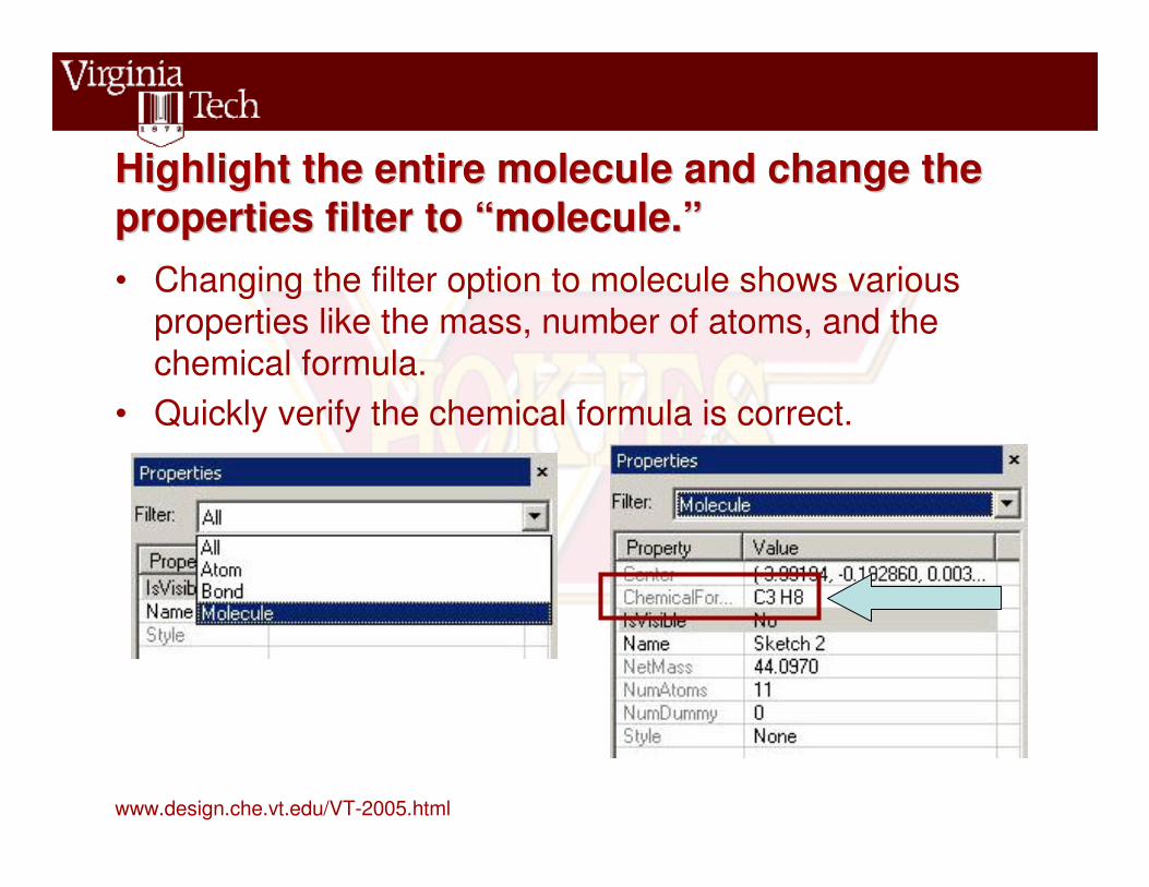
Highlight the entire molecule and change the Highlight the entire molecule and change the properties filter to “molecule.”properties filter to “molecule.”• Changing the filter option to molecule shows various

properties like the mass, number of atoms, and the chemical formula.

• Quickly verify the chemical formula is correct.


Now we use the “Clean” tool to correct the Now we use the “Clean” tool to correct the bond lengths and bond angles.bond lengths and bond angles.• Left click on the “Clean” tool icon on the toolbar.• The “Clean” tool does a rough geometry optimization

and adjusts the bond lengths and angles to the correct values for each atom and bond type.

• We are now finished constructing our example molecule, Propane.


Now we move onto setting up the Geometry Now we move onto setting up the Geometry Optimization calculation.Optimization calculation.• Select the “DMol3 calculation” from the “Modules”

Menu or use the icon on the toolbar.• The calculation dialog box will appear.


Select the task option in the DMol3 calculation Select the task option in the DMol3 calculation window.window.• Geometry optimization fixed the atomic coordinates for

the molecule by minimizing the total energy of the molecule.


Adjust the Geometry Optimization tolerance to Adjust the Geometry Optimization tolerance to “Fine.”“Fine.”• This can be done in the Setup or

Electronic tab.• This is the accuracy of the

Hamiltonian matrix element convergence.

• This specifies the accuracy to which the SCF (Self-Consistent Field) equations are converged. The “Fine” setting is recommended by the software documentation for highly accurate geometry optimizations. It represents a convergence of 10-6.


Select DNP as the Basis Set in the Electronic Select DNP as the Basis Set in the Electronic tab.tab.• DNP = Double Numerical basis with

Polarization functions, i.e., functions with angular momentum one higher than the highest occupied orbital in the free atom.

• According to the software documentation, “minimal basis sets are generally inadequate for anything but qualitative results, while DNP sets are the most reliable.” The DNP option instructs the program to ignore extraneous functions that “eliminate” certain atomic orbitals.

• When Quality it set to “Fine,” DNP is the default basis set.


Select GGA (local correlation) and VWNSelect GGA (local correlation) and VWN--BP BP (gradient(gradient--corrected functional) for the corrected functional) for the Functional option in the Setup tab.Functional option in the Setup tab.

• GGA = Generalized Gradient Approximation.• VWN-BP = BP functional (Becke, 1986; Pedrew, 1986)

with local correlation replaced by the VWN functional (Volsko, Wilk, and Nusair, 1980). Koch and Holthausen(2001) give excellent guidance about the selection of appropriate functionals.


Select the “More” button in the Job Control Select the “More” button in the Job Control tab.tab.• Check the “Retain server files” box. This will save

the files to the hard drive in the “jobs” directory.


Click the “Files” button at the bottom of the Click the “Files” button at the bottom of the DMol3 calculation dialog box.DMol3 calculation dialog box.• Click the “Save Files” button. This will create the input

files necessary for the calculation. They are visible in the Project window.


Open “propane.input” from the Project Open “propane.input” from the Project window.window.• Insert the code “Basis_version v4.0.0” into the input file. • This statement instructs the program to use version 4.0.0 DNP basis

set instead of the default v3.5 DNP basis set. The software documentation recommends v4.0.0 for COSMO calculations.


Leave the “Spin Unrestricted” box unchecked Leave the “Spin Unrestricted” box unchecked in the Setup tab.in the Setup tab.• Checking the “Spin Unrestricted” is necessary when

working with radicals, charged molecules, and organo-metallics.

• Although it is possible to run an organic molecule with the “Spin Unrestricted” setting, it will be much slower computationally.

• Checking the “Symmetry” box in the setup tab can also apply to certain molecules, but not all.


Click the “Run Files” button to begin the DMol3 Click the “Run Files” button to begin the DMol3 Geometry Optimization.Geometry Optimization.• The geometry optimization predicts the energy

level of the molecule in the ideal gas phase. • This calculation is the longest step of the

procedure and will require ~75% of the time to produce a sigma profile.


The Project window will show the files created The Project window will show the files created and tracks the progress of the calculation.and tracks the progress of the calculation.• The *.xsd file is the optimized

geometry. All further calculations should use this file.

• The *.outmol file will show the ideal gas phase energy. There are additional files that do not show up in the Project window but are stored in the “Jobs” folder. (C:\Program Files\Accelrys\MS Modeling 3.2\Gateway\root_default\dsd\jobs)


We have now completed the Geometry We have now completed the Geometry Optimization and will proceed to the COSMO Optimization and will proceed to the COSMO calculation.calculation.• Begin by opening the

geometry optimization output, vt-0003.xsd, and open another DMol3 calculation dialog box.

• Select the task, “Energy.”• Leave all other options the

same as the geometry optimization.


Click the “Files” button in the calculation Click the “Files” button in the calculation window.window.• Click the “Save Files” button to create the input

files.


Open the propane.input file and add the Open the propane.input file and add the COSMO calculation keywords.COSMO calculation keywords.• The COSMO keywords tell the program which parameters to use in

the COSMO calculation including atomic radii, basis set version, etc.


Now we review the parameters and settings in Now we review the parameters and settings in the COSMO keywords.the COSMO keywords.• This statement turns the

COSMO calculation on.• Again, we will use basis set

version 4.0.0 instead of the default v3.5.

• The first number is the atomic number and the second term is the fitted atomic radii. Klamt (1998) fitted these parameters to several sets of data.


Now we will run the COSMO calculation.Now we will run the COSMO calculation.

• Click on the “Run Files” button from the calculation window to begin the energy calculation.

• Upon completion, the Project window will contain a *.cosmo and *.outmol file. There are additional files stored in the “Jobs” folder.


The *.The *.cosmocosmo file contains much useful file contains much useful information.information.• This file contains the

volume of the cavityaround the molecule in the theoretical conducting medium, and it is used in the COSMO-RS/COSMO-SAC models.

• It also contains the condensed phase energy, the number of surface segments, and their charge.


We edit the *.We edit the *.cosmocosmo file to make it compatible file to make it compatible with the sigma averaging FORTRAN program.with the sigma averaging FORTRAN program.• Record the number of surface segments.• Delete all information above the last table, which

contains the segment charges and coordinates. • Then save as a *.txt text file.

Delete alltext abovethis line.


Our sigma averaging program uses the Our sigma averaging program uses the modified *.modified *.cosmocosmo file to calculate the sigma file to calculate the sigma profile. profile. • We average the surface charge densities from the

*.cosmo file to find an effective surface charge density on a standard surface segment.

2 2 2*

2 2 2 2

2 2 2

2 2 2 2

exp

exp

n av mnn

n n av n avm

n av mn

n n av n av

r r dr r r r

r r dr r r r

σσ

� �−� �+ +� �=

� �−� �+ +� �

�

�


The averaging program creates a new text file, The averaging program creates a new text file, the sigma profile.the sigma profile.• The output file is “ ‘Chemical name’ Sigma-profile.txt” is

located in the C:\Profiles\ directory. This directory must be created manually before running the averaging program.

• The output can be input directly into the COSMO-SAC program or can be plotted graphically.


We run the FORTRAN program to average the We run the FORTRAN program to average the surface charges over a standardized bonding surface charges over a standardized bonding site.site.• Run sigmaprofile.exe.• Follow the prompts and enter:

– New COSMO output (c:/propane.txt)

– Chemical Name (Propane)– The Number of Surface Segments


The sigma averaging program output is text, but The sigma averaging program output is text, but can be easily converted into graphical form.can be easily converted into graphical form.

Sigma values, (e/A2) [X-axis]

P(σσσσ) values, (A2) [Y-axis]


Using Microsoft™ Excel, we display the sigma Using Microsoft™ Excel, we display the sigma profile below.profile below.

Propane Sigma Profile

0

5

10

15

20

25

-0.025 -0.020 -0.015 -0.010 -0.005 0.000 0.005 0.010 0.015 0.020 0.025

Sigma, σσσσ e/A2

P( σσ σσ

)*A

rea(

σσ σσ),

A2

VT-0003 Propane


Acknowledgments Acknowledgments

• We want to thank Alliant Techsystems (particularly Anthony Miano, Vice President), AspenTech(particularly Dustin MacNeil, Director of Worldwide University Programs, Larry Evans, Board Chairman, and Chau-Chyun Chen), China Petroleum and Chemical Corporation (particularly Wilfred Wang, President) and Honeywell Specialty Materials and Honeywell International Foundation for supporting our educational programs in computer-aided design and process systems engineering at Virginia Tech. Michael Zwolak gratefully appreciates support from an NSF Graduate Fellowship.


ReferencesReferences

Andzelm, Jan; Klamt, Andreas; and Kölmel, Christoph, “Incorporation of solvent effects into density functional calculations of molecular energies and geometries,” J. Chem. Phys., 103, 9312-9321 (1995)

Bustamante, P.; Pena, M.A.; Barra, J., The Modified Extended Hansen Method to Determine Partial Solubility Parameters of Drugs Containing a Single Hydrogen Bonding Group and Their Sodium Derivatives: Benzoic Acid/Na and Ibuprofen/Na,Int. J. of Pharmaceutics, 2000, 194, 117.

Giles, Neil F. and Wilson, Grant M., “Phase Equilibria on Seven Binary Mixtures,” J. Chem. Eng. Data., 45, 146-153 (2000).

Klamt, Andreas, G. Shurmann, “COSMO-A New Approach


ReferencesReferences

Lin, Shiang-Tai; Chang, Jaeeon; Wang, Shu; Goddard III, William A.; Sandler, Stanley I., “Prediction of Vapor Pressures and Enthalpies of Vaporization Using COSMO Solvation Model,” J. Phys. Chem., 108, 7429-7439, (2004).

Lin, Shiang-Tai and Stanley I. Sandler, “A Priori Phase Equilibrium Prediction from a Segment Contribution Solvation Model”, Ind. Eng. Chem. Res, 41, 899(2002a).

Lin, Shiang-Tai and Stanley I. Sandler, “Reply to Comments on “A Priori Phase Equilibrium Prediction from a Segment Contribution Solvation Model,” Ind. Eng. Chem. Res., 41, 2332 (2002b).

Panayiotou, Costas, “Equation-of-State Models and Quantum Mechanics Calculations,” Ind. Eng. Chem. Res, 42, 1495 (2003).