


Languages
Pages
Legal


Copyright © 2015, ESSS, GDI, and RDI. All Rights Reserved. Page 1
(370-071015)
User Manual July, 2015
WWW.ROCKY-DEM.COM
安世
亚太
PERA Global

Page 2 Copyright © 2015, ESSS, GDI, and RDI. All Rights Reserved.
User Manual V 3.7.0
安世
亚太
PERA Global

Copyright © 2015, ESSS, GDI, and RDI. All Rights Reserved. Page 3
COPYRIGHT © 2015, Engineering Simulation and Scientific Software (ESSS), Granular Dynamics
International, LLC (GDI), and Rocky DEM, Inc. (RDI). ALL RIGHTS RESERVED.
No part of this documentation may be reproduced in any form, by any means, without the prior written
permission of ESSS, GDI, and RDI.
ESSS, GDI, and RDI make no representations or warranties with respect to the program material and
specifically disclaim any implied warranties, accuracy, merchantability or fitness for any particular purpose.
Furthermore, ESSS, GDI, and RDI reserve the right to revise the program material and to make changes
therein without obligation to notify purchaser of any revisions or changes except specific errors determined to
be incorporated in the program material. It shall be the responsibility of ESSS, GDI, and RDI to correct any
such errors in an expeditious manner. In no event shall ESSS, GDI, or RDI be liable for any incidental,
indirect, special, or consequential damages arising out of the purchaser’s use of program material.
Autodesk, AutoCAD, and Inventor are registered trademarks or trademarks of Autodesk, Inc., and/or its subsidiaries
and/or affiliates in the USA and/or other countries. Windows and Excel are registered trademarks of Microsoft Corporation
in the United States and other countries. Intel, Intel Core, and Xeon, are trademarks of Intel Corporation in the U.S. and/or
other countries. SolidWorks is a registered trademark of Dassault Systèmes SolidWorks Corporation in the United States
and overseas. Adobe Photoshop is either a registered trademark or a trademark of Adobe Systems Incorporated in the
United States and/or other countries. ANSYS, ANSYS Workbench, FLUENT and any and all ANSYS, Inc. brand, product,
service and feature names, logos and slogans are registered trademarks or trademarks of ANSYS, Inc. or its subsidiaries
in the United States or other countries. Python and PyCon are trademarks or registered trademarks of the Python
Software Foundation. All other brand, product, service, and feature names or trademarks are the property of their
respective owners.
安世
亚太
PERA Global

Page 4 Copyright © 2015, ESSS, GDI, and RDI. All Rights Reserved.
Contents
1. Software Overview .................................................................................................................................... 5
Program Features ...................................................................................................................................... 6
What's New ................................................................................................................................................ 8
System Requirements ............................................................................................................................... 8
Best Practices ............................................................................................................................................ 8
2. Getting Started ........................................................................................................................................ 12
Watch Overview Videos ........................................................................................................................... 12
Install/Remove Rocky .............................................................................................................................. 13
Understand the User Interface ................................................................................................................. 13
Set Your Rocky Preferences ................................................................................................................... 25
View Frequently Used Tasks ................................................................................................................... 37
Enter Input Variables or Mathematical Functions as Parameter Values .............................................................. 37 Enable Moving, Rotating, Vibrating, or Swinging Geometries .............................................................................. 38 Change the Speed of a Default Conveyor ............................................................................................................ 44 See Surface Wear on the Geometry Itself ............................................................................................................ 44
3. Setting Up a Simulation ........................................................................................................................... 47
Open a Simulation Project ....................................................................................................................... 47
Save a Simulation Project ........................................................................................................................ 47
Set Simulation Parameters ...................................................................................................................... 49
Verify Simulation Size ............................................................................................................................ 100
4. Processing a Simulation ........................................................................................................................ 102
Start a Simulation .................................................................................................................................. 102
Stop a Simulation ................................................................................................................................... 104
Process Multiple Simulations at Once ................................................................................................... 105
5. Analyzing a Simulation .......................................................................................................................... 106
View and Save Simulation Statistics...................................................................................................... 106
Create and Save an Animation .............................................................................................................. 106
6. Getting Help and Support ...................................................................................................................... 111
7. Appendices ............................................................................................................................................ 112
Appendix A: Particle Shape Examples .................................................................................................. 113
Appendix B: ASCII Printable Characters ............................................................................................... 116
Appendix C: Calculation Reference ....................................................................................................... 119
Appendix D: Use Variables to Test Varying Belt Speeds ...................................................................... 203
Glossary .................................................................................................................................................... 209
Index .......................................................................................................................................................... 210
安世
亚太
PERA Global

Copyright © 2015, ESSS, GDI, and RDI. All Rights Reserved. Page 5
1. Software Overview
Rocky is a 3D Discrete Element Method (DEM) modeling program that simulates how a particle group flows
around a boundary in a conveyor chute, mill, or other bulk materials handling design.
Engineers use Rocky to test and adjust
geometries based upon the metrics Rocky
provides. In this way, Rocky helps
manufacturing organizations:
Increase belt and liner life and
capacity
Eliminate blockages and liner
punctures
Decrease spillage and product
degradation
Reduce dust, noise, and belt power
Define ore trajectories
Optimize belt tracking
Minimize liner wear and maintenance
A typical scenario for Rocky usage is
provided in the flow diagram in Figure 1.
This section includes the following topics:
Program Features
What's New
System Requirements
Best Practices
Figure 1: Typical scenario for using Rocky software
安世
亚太
PERA Global

Page 6 Copyright © 2015, ESSS, GDI, and RDI. All Rights Reserved.
Program Features
Rocky is a powerful tool for evaluating the performance of your bulk flow handling geometries. The main
features included within this version of Rocky are described below. You can also review a list of Rocky
capabilities on the website here: http://rocky-dem.com/index.php?pg=capability.
Simulates particles of various shapes, sizes,
and combinations
Rocky uses realistic contact rheology, which
allows the choice from a nearly limitless
array of particle shapes, sizes, and
combinations, including faceted
polyhedrons, rods, pellets, and briquettes.
Replicates dry, wet, sticky, and dust-like
particles
Rocky uses a concept of “sticky particles” to
simulate how moist particles—such as clay—behave
differently than dry particles in a materials handling
design.
Processes simulations faster and with double
precision
Parallel scaling features enable Rocky to process
your simulations up to 25 times faster using up to
32 multi-core processors. Compared to single
precision, this provides superior contact mechanics
accuracy.
Simplifies simulation setup
User-friendly menus and dialogs allows quick
input of parameters. In addition, Rocky
includes over 100 editable parameters, which
allows for maximum customization.
Figure 2: Particle Laboratory Calibrations
安世
亚太
PERA Global

Copyright © 2015, ESSS, GDI, and RDI. All Rights Reserved. Page 7
Enables geometry import from a variety
of CAD programs
Rocky can import STL, XGL, and DXF
3D faces geometry files directly into the
software. This allows the user to see
how particles act upon on an exact
design while still enabling you to iterate
utilizing tools already in use.
Facilitates animated boundaries
Rocky has the capability to create
moving, rotating, swinging, and vibrating
boundaries, such as gates that lift and
rotate, or screens that vibrate, adding
another level of realism to the
simulations.
Modifies Geometries to Show Wear
Rocky includes functionality that
enables you to easily see how wear will
affect a geometry. Shear work applied
by particles will appear to dissolve
chute and mill liners right before your
eyes.
Displays results in easy-to-understand formats
Rocky uses different colors to represent how certain parameters and calculations—such as power draw,
shear intensities, and belt and liner wear—act upon the particles and boundaries in your design. This
enables you to see how the design performed even before the metrics and graphs are reviewed.
安世
亚太
PERA Global

Page 8 Copyright © 2015, ESSS, GDI, and RDI. All Rights Reserved.
What's New
Each new release of Rocky includes a list of what features and functionality have changed since the last
released version. This list is displayed automatically whenever you chose to upgrade your version. Or, to
review the list at any other time, from the Help menu, click Changelog.
System Requirements
Rocky has been designed to be used in conjunction with common CAD design tools, such as Autodesk
Inventor and AutoCAD. As a result, Rocky will have similar system requirements. Please see below for
minimum system requirements and optional recommendations.
Minimum Requirements:
64-bit Windows 7
A video card that supports OpenGL graphics
4 GB of free disk space
4 GB of RAM
Two-button mouse with center wheel
Screen resolution of 1280 x 1024
Recommended:
8 GB of free disk space
8 GB of RAM
Quad-core or better processor (Intel Core i5, Intel Core i7, or Intel Xeon processor)
A Nvidia GPU card with at least 4 GB memory and fast double-precision processing capabilities (Telsa
K40, Telsa K80, Titan, Titan Black, or Titan Z)
Autodesk Inventor or other CAD software
Microsoft Excel or other spreadsheet software
AVI-compatible media player
Best Practices
The engineers who developed and tested Rocky have compiled the following set of best practices to help you
get the most out of using the software. These recommendations are best used in conjunction with the user
assistance content that follows.
What would you like to learn about?
Best Practices for Faster Processing
Best Practices for Creating Geometries for Import
Best Practices for Setting up Geometries
Best Practices for Setting Up Particles
安世
亚太
PERA Global

Copyright © 2015, ESSS, GDI, and RDI. All Rights Reserved. Page 9
Best Practices for Faster Processing
The amount of time it takes for Rocky to process a simulation depends upon many factors, including but not
limited to:
The processing speed of the computer Rocky is running upon
The number, size, and complexity of the particles being simulated
The simulation time step, which is defined by particle size, density, contact loading stiffness(Young’s
Modulus), and restitution coefficients
The size of the geometries
The size of the boundary triangles
The simulation time (in seconds)
Whether the simulation files are being saved over a network
Whether you are using CPU or GPU processing capabilities
While there are no hard-and-fast rules regarding processing speed in Rocky, there are some steps you can
take. To speed up your processing time, do one or more of the following:
Use GPU processing and/or increase your processing power.
Reduce your particle stiffness. The default stiffness of 1x10⁸ Pa can be safely reduced to 1x10
6 -
1x10⁷ Pa for narrow size distributions (1:3 or less). This should result in a 3-10x increase in time
step.
Increase your minimum particle size.
Reduce the complexity (sides, corners, size distributions) of your particles.
Shorten the simulation length.
Increase the size of your boundary triangles. The default value of 0.1 is recommended for all
boundaries where you want to see wear data.
Run and save Rocky files locally; avoid processing and saving Rocky simulations over a network.
Run only one simulation at a time on any one machine.
To gain an understanding of how much faster GPU processing could be as compared with CPU processing,
see http://rocky-dem.com/index.php?pg=gpu_processing.
Best Practices for Creating Geometries for Import
Use the following recommendations when using a CAD program to create geometries for importing into
Rocky:
Orient your design around the origin. For example, when designing conveyor chutes, place the
center of the head pulley at (0,0,0), and build your other components around it.
Include the conveyors in your design but do not import them into Rocky. It is easier to use the
conveyors included with Rocky and only import your chutes or other geometries. Use the conveyor
dimensions in your CAD design to size and position the Rocky conveyors accordingly.
Make your design as realistic as possible. Use actual dimensions whenever possible.
Remove any “hidden” boundaries before saving the file you want to import. Some hidden geometries
might be imported into Rocky.
安世
亚太
PERA Global

Page 10 Copyright © 2015, ESSS, GDI, and RDI. All Rights Reserved.
Color boundary components differently to make it easier to distinguish components before and after
import.
Best Practices for Setting up Geometries
Use the following recommendations when setting up geometries in Rocky:
Only import your non-conveyor geometries into Rocky (i.e., your chute or mill). Use the conveyor
designs included within Rocky for your conveyor components.
Make the conveyor settings as realistic as possible. Any error or shortcut taken in setting up
geometries will result in false data.
Ensure that the triangle size of your feed and receiving conveyors are small enough to avoid
deformation of the geometries. Larger triangle sizes (1m for example) might change the overall
shape of the conveyor, making your simulation less realistic. It is recommended that the default value
of 0.1 be used.
Note: Triangle size will not affect the shape of custom (imported) boundaries; just the conveyors
included with Rocky.
Ensure that your inlet is large enough to allow your largest particle to pass through, but still slightly
smaller than your geometry opening. This will help prevent particles from getting "stuck".
When setting up multiple inlets, ensure that your inlet locations and Start and Stop Times are
configured in such a way as to avoid particle groups from overlapping during the simulation. An inlet
will delay releasing its particles until no other particles from other particle groups are in the way.
Note: This step is unnecessary if Release Particles without Overlap Check is selected on the
Solver/General Settings tab. (From the Data panel, click Solver and then from the Data Editors panel,
select General Settings on the Solver tab.)
When locating an inlet or default conveyor, first sketch its size and location in a CAD program and
then use the resulting coordinates to properly place it within Rocky.
Ensure that particle speed equals belt speed by the time the particles reach the pulley. Adjust the
loading length of the belt to achieve the desired result.
When setting up custom feeder boxes, ensure that there is enough vertical space between the wall of
the box and the entry point of the particles (i.e. top of the feeder box or inlet) for your largest particle.
If a particle hits a boundary or other particle before fully entering the simulation, all particles will stop
flowing.
Note: This step is unnecessary if Release Particles without Overlap Check is selected on the
Solver/General Settings tab. (From the Data panel, click Solver and then from the Data Editors panel,
select General Settings on the Solver tab.)
To prevent this from happening, do one of the following (see also Figure 3 below):
Make your inlet smaller.
Add a vertical lip to the top of your feeder box.
安世
亚太
PERA Global

Copyright © 2015, ESSS, GDI, and RDI. All Rights Reserved. Page 11
Best Practices for Setting Up Particles
Use the following recommendations when setting up particles in Rocky:
When setting particle friction values:
o For rock or granular particles with rougher surfaces, set friction values to 0.6 - 0.7
o For glass-like particles with smoother surfaces, set friction values no lower than 0.3
When testing out a new chute design, save time by running a quick simulation with round (sphere)
particles to ensure your boundary settings are as you want them. This will take less time and will
enable you to iterate on your design faster. Once your boundaries are set and verified, set up your
non-round particle combinations and distributions and run that as a final step.
Figure 3:
(1) Angled walls of feeder box
prevents particle from fully
entering simulation area;
(2) Make the inlet smaller;
(3) Add a lip to the top of the
feeder box. 安世
亚太
PERA Global

Page 12 Copyright © 2015, ESSS, GDI, and RDI. All Rights Reserved.
2. Getting Started
Use the following information to get started with Rocky and gain an understanding of its various features and
components.
What would you like to do?
Watch Overview Videos
Install/Remove Rocky
Understand the User Interface
File Types
Set Your Rocky Preferences
View Frequently Used Tasks
Watch Overview Videos
To get you started with using the most frequently used features and functionality available within Rocky, our
team has prepared some high-level overview and how-to videos. These videos will be later supplemented
with more in-depth written user assistance content, but for now these videos are a good place to start
learning about the product and its features and capabilities.
To view a video
1. Log into the ESSS customer portal.
Note: If you do not have access to the customer portal, please contact [email protected]
for assistance
2. Click the link below to open the video you want to watch.
How to install Rocky: This 10 minute video provides a detailed look at the steps required to install
Rocky and configure the floating licensing server. It is best watched in conjunction with the
written instructions for configuring the Rocky 3 floating licensing server.
User interface overview: This 5 minute video outlines the major parts of the Rocky user interface,
including the menu and tool bars, Data and Data Editors panels, and the various visualization
options available.
Customizing the Rocky User Interface: This 5 minute video goes over the five main components
of the Rocky UI, and how you can show, hide, move, and resize them to your liking.
Data panel overview: Outlines the various components of the Data tree, the hierarchical
component that a Rocky simulation is built upon. Right-clicking items in the Data panel displays a
contextual menu with available actions for the selected item; Left-clicking items in the Data panel
displays editable options in the Data Editors panel, which is located just below the Data panel.
Rocky Preferences Overview: Goes over the various global preferences that can be set in Rocky
including data and time formats, timestep formats, and various visualization settings.
Geometries and Particles as Grid Parts: Shows how Geometries and Particles are displayed in
Rocky 3D Views, and how changing visualization options changes the coloration to show
different results.
安世
亚太
PERA Global

Copyright © 2015, ESSS, GDI, and RDI. All Rights Reserved. Page 13
Using the Timestep Toolbar Options: Shows how using the arrows, drop-down list, and playback
button on the Timestep toolbar enables you to see progressive results in the Workspace. Also
shows how a workspace can be divided up into many different 3D Views and plots.
Selecting Multiple Options in the Data Panel: Shows the multiple select feature in Rocky that
enables you to select multiple items in the Data panel and edit all common parameters at once in
the Data Editors panel.
Opening a Simulation: Shows the various ways you can start a new simulation or edit an existing
one.
Creating a graph (curve or plot): Shows some ways to display and analyze simulation results in
Rocky, including creating curves and plots.
Editing a graph (curve or plot): Demonstrates some ways to change or modify an existing plot or
curve within Rocky.
Changing the 3D View: Demonstrates how to use the toolbar buttons, mouse and keyboard to
change the perspective, zoom, rotate, and pan a 3D View in the Workspace.
Using User Processes to Analyze a Component: Shows how using the User Processes features,
including the Plane and Cube options, enables you to divide your geometries to analyze specific
sections or components.
Importing Custom Geometry: Shows how to add your own geometry components into Rocky, and
also covers the file options supported.
Creating an Animation: Shows how to set up an animation of your simulation and save it as an
AVI.
Install/Remove Rocky
Instructions for how to install or remove Rocky and also configure the floating licensing server are provided
below.
Note: You must be logged into the ESSS customer portal to view the content. If you do not have access to
the customer portal, please contact [email protected] for assistance.
To install ROCKY
1. View the overview video on How to install Rocky.
2. Follow the written instructions for configuring the Rocky 3 floating licensing server.
To remove ROCKY
1. From the Start menu, click All Programs, click ESSS, click Rocky 3, and then click Uninstall Rocky 3.
2. Follow the instructions provided on your screen.
Understand the User Interface
Rocky is a powerful program with a flexible, hierarchical interface. One main screen gives you access to the
most frequently used functions and features, and provides you with various views of the simulation.
Additional panels allow you to access properties and settings to fine-tune your simulation and view statistics
based upon the results.
安世
亚太
PERA Global

Page 14 Copyright © 2015, ESSS, GDI, and RDI. All Rights Reserved.
What would you like to learn about?
Main UI Components
Hidden Features
Keyboard Accessibility and Shortcuts
File Types
Main UI Components
Use this section to explore the five major parts of the Rocky user interface, and learn when and why you
might access them.
Figure 4: The five main components of the Rocky User Interface
Menu and Toolbar
The menu and toolbar are located at the very top of the Rocky main screen. From here, you can begin a new
simulation, open an existing simulation, save a new simulation, show/hide Rocky panels, organize Rocky
windows within the Workspace, access Help, and more.
安世
亚太
PERA Global

Copyright © 2015, ESSS, GDI, and RDI. All Rights Reserved. Page 15
While the menu is static in its location, the various sections that make up the toolbar can be moved or made
to float independent of the screen by clicking a toolbar handle and then dragging it and dropping it with the
mouse.
You can also show/hide toolbars by right clicking a toolbar and selecting or deselecting the options at the
very bottom of the contextual menu.
Panels
Below the toolbar and surrounding the Workspace are various floating panels that enable you to set
parameters and choose options for your simulation and its resulting data. The primary panels for configuring
your simulation are the Data and Data Editors panels that appear (by default) to the left of the Workspace;
the primary panels for post-processing are the Windows and Windows Editors panels that appear (by default)
to the right of the Workspace. Also showing (by default) to the right of the Workspace, you can display
various tools panels such as Animations or Macros. You can choose to show/hide multiple panels through
both the View and Tools menus located at the top of the screen.
All panels in Rocky can be resized, moved, nested with other panels, and undocked to float independent of
the Rocky main screen. Specifically:
To resize a panel, hover your mouse over a panel boundary until the resize icon appears. Then, click
and drag the boundary to the desired width or height.
To move a panel to another docked location, click the panel title and drag to the desired area outside
of the Workspace. While still dragging the panel, a preview of new docked locations will be displayed
with a blue background. To select a new docked location, release the mouse over the preview of the
location you want.
To make a nested panel, click the panel title and then drag it directly over another panel until the
lower panel is blue, and then release the mouse. The second panel will appear as a tab at the bottom
of the first panel. Select the tab you want to toggle between panels.
To make a docked panel float, click the panel title, drag it towards the center of the screen then
release the mouse. Alternatively, you can also click the icon to the left of the panel’s close button to
make any docked panel float.
Show/hide multiple panels by right clicking a panel’s title bar and selecting or deselecting the options at the
top and middle of the contextual menu. To learn more about showing, hiding, moving, and resizing objects in
the Rocky UI, watch the Customizing the Rocky User Interface video.
Workspace
A Workspace is a collection of Rocky windows. Located in the center of the Rocky screen, the windows that
make up a Workspace are where you choose to view the physical components of your simulation setup (3D
View windows), and interact with the graphical results of your simulation (plot and histogram windows).
You can have multiple Workspaces for different purposes, such as by analysis type. These are designated by
Workspace tabs along the bottom of the Workspace area, which can also be renamed to better help you
organize your data.
安世
亚太
PERA Global

Page 16 Copyright © 2015, ESSS, GDI, and RDI. All Rights Reserved.
Window
A window in Rocky is the method by which the physical components or the graphical results of the simulation
are viewed. Windows appear only from within a Rocky Workspace, but you can maximize the size of the
Window to take advantage of the entire Workspace area, or you can tile several windows in columns by using
the options at the bottom of the Windows menu.
There are six different types of windows in Rocky as described below:
3D View: Displays the physical geometries of your simulation and shows you a preview of your
animations.
Cross Plots: Graphically compares multiple measurements made at a single time or location along
two or more axes.
Histograms: Displays in a bar graph data ranges that you select from the Grid Functions or Grids
tabs.
Time Plots: Graphs data across a time period. Also enables you to inspect a particular point in a
curve and see the results in table format.
Multi-Time Plots: Like Time Plot, graphs data across a time period but enables multiple plots to be
compared in one window.
Space Plots: Graphs one-dimensional (line) data from the Grid Functions tab.
Hidden Features
This section covers the not-so-obvious but useful features scattered throughout the Rocky UI and how it
might benefit you to use them.
What would you like to do?
Name Components to Affect Sort Order
Show/Hide Components by Using Eye icons and Checkboxes
See Input/Output Relationships in the Data Panel When Component Names are Bold
Determine the Frequency of Calculations by Pinning/Unpinning Items
Recognize Data Placeholders
Double-Click the Status Panel to Jump to the Appropriate UI Location
Use Colored Text to Validate the Syntax
Drag/Drop Items into Windows
Access the Right-Click Menu for Additional Features
Use the Data Panel Search Bar to Quickly Find Components
Refer to the Rocky Title Bar for Simulation Progress Details
Name Components to Affect Sort Order
Sorting in Rocky follows the rules for Extended ASCII character codes (For a full list, see Appendix B: ASCII
Printable Characters.) In general, Names beginning with spaces are sorted first, followed by most special
characters, followed by numbers, followed by uppercase letters, and ending with lowercase letters.
安世
亚太
PERA Global

Copyright © 2015, ESSS, GDI, and RDI. All Rights Reserved. Page 17
For example, Rocky would sort the following 12 geometry components in the order shown in Figure 5.
Figure 5: Example sort order in Rocky
Show/Hide Components by Using Eye icons and Checkboxes
Rocky provides two complementary methods for determining whether a component or family of components
will be shown or hidden in the Workspace: The eye icon (Figure 6), which affects the visibility of only that
individual component, and the checkbox (Figure 7), which affects the visibility of all sub-components beneath
the object.
Figure 6: Open and closed eye icons to the right of objects in the Data panel
安世
亚太
PERA Global

Page 18 Copyright © 2015, ESSS, GDI, and RDI. All Rights Reserved.
Figure 7: Checkboxes to the left of objects in the Data panel
Eye Icon
An “open” eye icon (default setting) indicates that particular object is visible or shown in 3D View windows,
plots, or histograms. A “closed” eye icon keeps that item in the simulation's calculations but makes the object
appear invisible or hidden in the window. This is useful for seeing behind one object to another in an
animation, for example, or for focusing on a particular curve in a plot.
Checkbox
In the Data panel, the checkbox has the same visibility affect as the eye icon but is hierarchical, meaning it
affects all children components directly beneath that item in the Data panel. For example, clearing the
checkbox to the left of Geometries hides all individual geometry components listed beneath it.
In the Windows panel, the checkbox acts like the eye icon does in the Data panel: it shows/hides the
individual object—in this case, various windows in the Workspace. Unlike in the Data panel, checkboxes in the
Windows panel are not hierarchical.
See Input/Output Relationships in the Data Panel When Component Names are Bold
Linked objects refers to the ability of a geometry component, Particles, or Air Flow to provide data to a
particular User Process, thus establishing an input/output relationship between them. This linkage is
illustrated in the Data panel by the name of the object providing the data (output) turning bold when the User
Process that is accepting the data (input) is selected, as shown in Figure 8.
安世
亚太
PERA Global

Copyright © 2015, ESSS, GDI, and RDI. All Rights Reserved. Page 19
Figure 8: Example of a geometry component shown in bold when the user process linked to it is selected
To create this kind of input/output relationship, the User Process must be created directly from the object
providing the data. In the example above, the “Cube <01> user process was created by selecting the
83.BC06 geometry and then creating a Cube user process from either the Data Editor or right-click menu.
Determine the Frequency of Calculations by Pinning/Unpinning Items
After processing your simulation, you can view various types of data on the Grid Functions and Curves tabs
for your simulation settings like particles and geometry components. Each of the items listed on these tabs
has a pin icon to the left of it, as illustrated in Figure 9.
Figure 9: Pin icons on the Grid Functions tab of the Data Editors panel
The color of these pin icons indicates how often Rocky calculates the particular item, as follows:
安世
亚太
PERA Global

Page 20 Copyright © 2015, ESSS, GDI, and RDI. All Rights Reserved.
A gray-colored pin (default) indicates that the item will not be calculated for any timestep. Choosing
to avoid calculating data that you don’t need saves processing time and power during your
simulation.
A red-colored pin indicates that the item will be calculated for each timestep included in the
simulation. And if settings affecting those values change, Rocky will recalculate to keep all the values
current.
Important: Choosing to have Rocky calculate the item at each timestep is likely to take up a
significant amount of processing time and power. Only choose to pin items for which having all
timestep calculations be kept up-to-date and available are truly necessary for your analysis.
Tip: To pin or unpin an item, just click left-click the pin icon.
Alternately, you can choose to have Rocky calculate any values you are interested in once, by right-clicking
the item and choosing Compute Statistics. This enables you to see values you are interested without taking
up as much processing time and power as it would take to pin the same item. The results you get are
dependent upon what kind of data item you chose, as described below:
For items on the Grid Functions tab, choosing to Compute Statistics results in only the current
timestep being calculated.
Note: Ensure first that Instantaneous is selected from the Time Scope drop down before taking this
step.
For items on the Curves tab, choosing to Compute Statistics results in all currently available
timesteps being calculated. But unlike pinning an item, choosing to Compute Statistics will not
continue to recalculate those values should settings change that affect them, or if new timesteps are
added to the simulation.
Recognize Data Placeholders
Rocky uses several different characters and strings as placeholders for calculations or explanations that
would take up too much room in the UI. Here is a quick list of some placeholders you might run across and
what they mean.
Note: These placeholders might appear on the Grid, Grid Functions, or Curves tabs (Data Editors panel) for
particles and geometry components.
Placeholder Description
? Information isn’t calculated yet. Same as “Not loaded.”
Not loaded Information isn’t calculated yet. Same as “?
- Not enough information available at this particular timestep in order to calculate the
values. Same as “Unable to calculate”.
Unable to calculate Not enough information available at this particular timestep in order to calculate the
values. Same as “-”.
Unknown Not enough information is known to calculate the value.
<ind> Item contains no units for the value displayed. Generally indicates a count of
something.
安世
亚太
PERA Global

Copyright © 2015, ESSS, GDI, and RDI. All Rights Reserved. Page 21
Double-Click the Status Panel to Jump to the Appropriate UI Location
If you have errors listed in the Status panel (Figure 10), you can double-click those errors to be taken to the
location in the Data panel where you would address them.
Figure 10: Example of errors shown on the Status panel
For example, if you double-click the “There are no geometries in the simulation” error, Rocky would enable
the Geometries item in the Data panel.
Use Colored Text to Validate the Syntax of Your Entries
Rocky provides instant feedback for entering functions and variables into a parameter text field by coloring
the text as you type, as explained below:
Red text indicates that the syntax of the active entry isn’t yet valid. The syntax is based upon the
rules of the Python programming language. It will tell you whether you have an open parenthesis that
needs to be closed, for example.
Green text indicates that the syntax of the active entry is valid.
Note: Green text does not indicate that the value, function, or variable of active entry has been
formatted correctly or is itself a valid entry. Validation happens after either pressing Enter or clicking
away from the text field.
Black text indicates a currently inactive entry.
Drag/Drop Items into Windows
There are several tasks in Rocky that can be accomplished more easily by dragging items with your mouse
and dropping them to another location, as described below:
Creating new views of Particles, individual geometry components, or Airflow: From the Data panel,
select the component(s) you want to view and then drag and drop them to a window of your choice
(3D View, Histogram, or Time Plot). Only the component(s) you selected will be added.
Creating new views of data sets: From the Data Editors panel, on the Curve or Grid Function tab,
select the data item(s) you want to show and then drag and drop them into the window type you
want (3D View, plots or histograms).
Creating multiple Multi-Time plots in a single window: After adding your first data set, hold the Ctrl
key while selecting your next data set and then drag and drop it into the gray area of an existing
Multi-Time plot window. Another plot appears in the same window.
Tip: You can also multi-select items to drag and drop. (For example, show multiple geometry
components at once in a 3D View.) Just hold the Ctrl or Shift key while left clicking your selections with
the mouse, and then drag and drop as usual.
安世
亚太
PERA Global

Page 22 Copyright © 2015, ESSS, GDI, and RDI. All Rights Reserved.
Access the Right-Click Menu for Additional Features
There are a few things in Rocky that can only be accomplished by right-clicking the item, as described below:
Adding/Importing geometry components: From the Data panel, right-click Geometries to access the
menu that enables you to add or import new geometry components.
Computing statistics for only the current Timestep: From the Data Editors panel, on the Curve or Grid
Function tab, right-click the data item you want to view values for and then click Compute Statistics
from the right-click menu.
Showing only a few components in a new window: From the Data panel, select the item(s) you want
displayed in a new window, right-click your selection, and then from the right-click menu, point to
Show in New and then click the window type you want. Only the items you selected appear in the
new window.
Import your own User Process shape for particle analysis: From the Data panel, right-click Particles,
point to User Processes, and then click Polyhedron (Envelope). From the Select the STL file for the
polyhedron dialog, navigate to the STL file you want, and then click Open. The Polyhedron you
chose appears under the User Processes list.
Note: You can also create a custom-shaped User Process from any existing User Process that was
originally created from a Particle group. (See also See Input/Output Relationships in the Data Panel
When Component Names are Bold.) From the Data panel, under User Process, right-click a User
Process that was created from a Particle group and then follow the instructions above.
Use the Data Panel Search Bar to Quickly Find Components
The search bar is located at the very top right of the Data panel, as shown in Figure 11.
Figure 11: Data panel search bar
When you start typing into it, Rocky immediately displays in the Data panel the entire hierarchy of the
component(s) that best match what you typed. In a simulation setup with many different components, using
the search bar can help you find what you need faster than scrolling.
Tips:
To search the names in order from left to right, enter the first few characters of the component you
want to find.
For example, to find all components that begin with “belt,” type belt into the search box. You would
find “belt 01” and “belt 02” but not “feeder belt” by using this method.
安世
亚太
PERA Global

Copyright © 2015, ESSS, GDI, and RDI. All Rights Reserved. Page 23
To search anywhere in the name, type an asterisk (*) followed by the characters anywhere within the
name that you want to find.
For example, to find all components containing “belt” anywhere in the name, type *belt into the
search box. In this way, you would find the “feeder belt” component as well as “belt 01” and “belt 02.”
Refer to the Rocky Title Bar for Simulation Progress Details
When you are actively processing a simulation (see Start a Simulation), the Title bar for the Rocky program
displays useful details about the simulation’s progress.
Figure 12: Example of Title bar progress information shown while a simulation is processing
This progress information in the Title bar includes the following:
Output: The total number of Timestep files that have been saved thus far. In the example in Figure
12, the total number of output files is 27.
Current progress: The particular second of the total Simulation Duration that Rocky is currently
calculating. Note that Rocky calculates in finer detail than is typically determined by the Output
Frequency in which it saves Timestep files. (See also Table 10: Solver, Time Configuration
parameter options). In the example in Figure 12, though Rocky is currently calculating for second
1.362, because the output frequency is set to 0.05 seconds, it won’t actually save a 28th
Timestep
representing 1.4 seconds until the current progress reaches that point.
Elapsed: Amount of real time since starting (or resuming) the simulation processing. In the example
in Figure 12, 14 seconds have elapsed since the simulation was resumed.
ETA: Rocky’s estimate of how much real time the simulation will take to complete. This is a rough
approximation Rocky extrapolates based upon the amount of time the last several timesteps took to
calculate. In the example in Figure 12, Rocky estimates that it will take roughly five hours for the 20
second simulation to complete. The ETA will get longer as more and more particles enter the
simulation and it takes more time for Rocky to calculate each timestep. Should the simulation reach a
point where more particles leave the simulation than enter it, the ETA will begin to get shorter.
Keyboard Accessibility and Shortcuts
While Rocky was not designed for full software accessibility, it does offer some limited features for keyboard
control. For example:
TAB key: Press to move from option to option within a Rocky dialog or panel.
SPACEBAR: Press to select or clear a check box, or to select buttons in panels.
UP/DOWN ARROW keys: Press to select list items within a Rocky dialog, Panel, or menu.
LEFT/RIGHT ARROW keys: Press to view different menus or to move horizontally in Rocky dialogs.
ESC key: Press to close a dialog.
ENTER: Press to select a button within Rocky dialogs.
安世
亚太
PERA Global

Page 24 Copyright © 2015, ESSS, GDI, and RDI. All Rights Reserved.
To view the full keyboard shortcut list
1. From the Options menu, click Preferences.
2. From the Preferences dialog, under Properties, click Shortcuts.
File Types
There are several unique file types used in Rocky, and several common ones. Use the table below to identify
when and why certain file types are used.
Note: Only the simulation project file is saved to the directory location you choose. All other files created by
Rocky (marked as “System” below) are saved to a project subfolder created automatically within the same
directory as your project file. System files are critical for Rocky functioning and should not be edited, moved,
or deleted.
Files you choose to export out of Rocky, including animation, image, and data files, are saved to the locations
you specify. See the below table for more detail.
Table 1: File Types Used in Rocky
Type Description Extension
Rocky Simulation Files
Simulation project file Used for storing parameters set for a particular simulation and is
also linked to the simulation Timestep files (.rhs) that are created
during processing.
One project file is saved for each simulation.
Opening a project file will display the last Timestep (.rhs)
file that was saved.
.rocky30
(System)
Simulation file
Used for storing information related to the results of the simulation. .rcy
(System)
Simulation Timestep file
During Processing, one Timestep file is saved per output
frequency; many Timestep files make up a whole simulation.
Timestep files are accessed by opening the project file
(.rocky30) file and then moving the Timestep slider in the
toolbar to the location you want.
Displaying a Timestep file shows the image (in a 3D View)
or data (in a plot or histogram) for that particular moment
in the simulation.
.rhs
(System)
Solver file
Used for storing information related to solving the simulation. .rocky20
(System)
Solver log file
Records the progress of the solver. .rocky20.log
(System)
Rocky log file
Records information about Rocky useful for error solving
purposes.
.rocky20.out
安世
亚太
PERA Global

Copyright © 2015, ESSS, GDI, and RDI. All Rights Reserved. Page 25
Type Description Extension
(System)
Rocky script file
Contains scripts and functions that enable Rocky to run properly. .rocky20.prg
(System)
Current Timestep file
This is where ROCKY saves what Timestep file is most current. _H.txt
Files Exported Out of Rocky
Simulation statistics file File created by exporting curves from a plot or histogram, and
which can be opened and edited in a spreadsheet program, such
as Microsoft Excel.
.csv
Animation file File created by exporting an animation, and which can be used for
viewing a simulation outside of Rocky.
.avi
Image file Used for saving or exporting a snapshot of what is currently being
displayed in a window on the Workspace, or for importing into
Rocky as a logo to be shown in the 3D View.
.png
.jpg
.bmp
Files Imported Into Rocky
Inventor file Used for importing geometries into Rocky.
Provides a more realistic image when compared with .stl.
.xgl
Inventor, AutoCAD, and
SolidWorks files
Used for importing geometries into Rocky.
Provides a less realistic image when compared with .xgl.
.stl
AutoCAD file Used for importing 3D Faces geometry files into Rocky. .dxf
FLUENT Case File Used for importing geometries from ANSYS FLUENT into Rocky.
Contains the grid, boundary conditions, and solution parameters
for a problem. Geometry component names will be retained when
importing a CAS file into Rocky.
.cas
FLUENT Mesh File Used for importing geometries from ANSYS FLUENT into Rocky.
Geometry component names will not be retained when importing a
MSH file into Rocky.
.msh
Set Your Rocky Preferences
There are several parameters you can set in Rocky that will affect your overall simulation. These include
various preferences and unit types, as well as catalogs and variables. These items can be determined before
you set up your simulation, or can be modified at any point during the setup process.
What would you like to learn about?
Setting Your Global Preferences
Setting Your Unit System
Defining Your Variables
Setting Your Application Catalog
安世
亚太
PERA Global
Page 26 Copyright © 2015, ESSS, GDI, and RDI. All Rights Reserved.
Setting Your Global Preferences
Global preferences for Rocky include settings like memory usage, date and time format, and plot and view
options. What you choose to set in preferences will affect the rest of the Rocky user interface.
To set your global preferences
1. From the Options menu, click Preferences.
2. From the Preferences dialog, choose the category you want under Properties, and then make the
choices you want on the right.
Note: Shortcuts aren’t currently editable.
3. Click Apply to save your changes.
4. Repeat steps 2-3 until you have set all the options you want, and then click OK to close the dialog.
Setting Your Unit System
Before you begin using Rocky, it is important that you understand the units used in the user interface and set
them the way you want. Currently, there are two unit systems included in Rocky: the International System
and the English. You can use choose to use one of these two included systems, or you can create your own
custom unit system.
Whatever system you choose will provide the default unit settings for all parameters used within Rocky.
However, each individual parameter unit can still be changed manually to another unit type at any time.
Use the images and tables below to help you understand your unit system options.
安世
亚太
PERA Global

Copyright © 2015, ESSS, GDI, and RDI. All Rights Reserved. Page 27
Figure 13: Unit Management dialog
Table 2: Unit Management dialog options
Setting Description Range
Unit System Sets the unit system used by default throughout
Rocky. Choices include:
International System: Units based upon
the International System of Units (SI).
English Units: System based on the
customary units of measurement used in
the United States.
If you have created custom unit systems, those
will display in this list also.
Lists all default and custom unit
systems for Rocky.
Category Lists the descriptive name of the item being
measured.
Automatic
Unit Provides the unit symbol that will be used by
default for the parameters in Rocky. These are
editable when you choose to create a custom
system.
Automatic
安世
亚太
PERA Global

Page 28 Copyright © 2015, ESSS, GDI, and RDI. All Rights Reserved.
Table 3: Default Units Used in Rocky
Item International Unit International
Unit Symbol English Unit
English
Unit
Symbol
Acceleration Linear meter per second
squared
m/s2 foot per second squared ft/s
2
Angular
Acceleration
radian per second
squared
rad/s2 radian per second squared rad/s
2
Angular Velocity radian per second rad/s radian per second rad/s
Area square meter m2 square foot ft
2
Density kilogram per cubic
meter
kg/m3 pound mass per cubic foot lbm/ft
3
Dynamic Viscosity Pascal second Pa·s centipoise cP
Force Newton N pound force lbf
Frequency hertz Hz hertz Hz
Isothermal
Compression
cubic meter per joule m3/J cubic meter per joule m
3/J
Length meter m foot ft
Mass kilogram kg pound mass lbm
Mass Flow Rate
(formerly
“Tonnage”)
metric tons per hour t/h metric tons per hour t/h
Mass per Energy kilogram per joule kg/J pound mass per British
thermal unit
lbm/Btu
Moment of Force
(formerly “Torque”)
Newton meter N·m foot pound force lbf·ft
Moment of Inertia kilogram meter squared kg·m² square foot pound mass lbm·ft2
Plane Angle degree dega degree dega
Power watts W horsepower hp
Pressure Pascal Pa pascal Pa
Specific Energy joules per kilogram J/kg British thermal unit per
pound mass
Btu/lbm
Specific Power watts per kilogram W/kg watts per kilogram W/kg
Time second s second s
Velocity meter per second m/s feet per second ft/s
Yield Stress force per unit area N/m2 pound force per square inch lbf/in
2
安世
亚太
PERA Global

Copyright © 2015, ESSS, GDI, and RDI. All Rights Reserved. Page 29
To select a unit system to use throughout Rocky
1. From the Options menu, click Unit System Manager.
2. From the Unit Management dialog, choose the option you want from the Unit System list, and then click
Close.
To create a new unit system
1. From the Options menu, click Unit System Manager.
2. From the Unit Management dialog, do one of the following:
To create a new unit system based upon an existing one, choose the option you want to copy from
the Unit Systems list, and then click the Copy the current Unit System button.
A copy of the existing system is created.
To create a new blank system, press the Create a new Unit System button.
A blank system is created.
3. Click the Rename the current Unit System button and then in the Enter the new name box, type the name
you want, and then click OK.
4. Edit the system list as you want.
To edit a custom unit system
1. From the Options menu, click Unit System Manager.
2. From the Unit Management dialog, choose the custom unit system you want to edit from the
Unit System list.
Note: You can only edit custom unit systems that you’ve added. If you want to edit the International or
English system units included in Rocky, you must first make a copy of those systems and then edit the
copy.
3. Do one or more of the following:
To change the units used, choose the option you want from the Unit list.
To add a new category, click the Add button, and then from the Add Category dialog, choose the
options you want in the Category and Unit lists, and then click OK.
To remove a category, select the category you want to remove and click the Remove button.
To remove a custom unit system
1. From the Options menu, click Unit System Manager.
2. From the Unit Management dialog, choose the custom unit system you want to remove from the Unit
System list, and then click the Remove the Current Unit System button.
Note: You can only remove custom unit systems that you’ve created. The International and English
system units included in Rocky are not removable.
Defining Your Variables
The Expressions/Variables tool in Rocky enables you to define unique placeholders for both Input variables
(values used within the Rocky set up parameters) and Output variables (values that are exported out of
安世
亚太
PERA Global

Page 30 Copyright © 2015, ESSS, GDI, and RDI. All Rights Reserved.
Rocky into programs like ANSYS Workbench for tasks like structural analysis). The variables you define can
then be used in place of actual numerical values. This is useful in cases where you have common values that
are linked (all belts are to be the same width, for example), and/or the values you enter might be changing
later in the setup (you want to experiment with three different belt speeds, for example).
For Input variables, you can enter into the parameter text fields a variable name on its own, or you can use a
variable within a mathematical function that you enter into the parameter text field instead. In this way, Rocky
enables you to create dynamic relationships between parameters, and enables you to change and update
placeholder values quickly. (For a more detailed example, see Appendix D: Use Variables to Test Varying
Belt Speeds).
Because it can be hard to remember what parameters use what variables, Rocky uses the Expressions list to
help you keep track of where the Input variables are being referenced—even if it is being used within a
function or other variable definition. The Expressions list is also useful for verifying what units the variable or
function is using for the particular location specified, and for changing the value or units of the variable later
without having to locate it again in the Data Editors panel.
Important: Verify that your field units are set the way you want before using or creating a variable—or function
including a variable—within a field. Even though variables are saved in the Variables list without units, as soon
as a variable—or function including a variable—is used within a parameter field, it takes on whatever units are
currently set for that field and those units are then recorded for that specific usage in the Expressions list.
Changing the units for the field after the variable or function have already been entered only converts the
numerical display to reflect the new units; the original variable or function amount and units are still retained.
However, you can change the units and value later by editing it in the Expressions list.
Variables can be defined and used at any point during the setup portion of your simulation. See also Enter
Input Variables or Mathematical Functions as Parameter Values.
Use the images and tables below to help you understand how to set your variables.
安世
亚太
PERA Global

Copyright © 2015, ESSS, GDI, and RDI. All Rights Reserved. Page 31
Figure 14: Example of entering a variable into a text field
Figure 15: The variable name and units used for the field appears after double-clicking the field
Figure 16: The current value for the variable entered appears in the field after clicking away from the field
安世
亚太
PERA Global

Page 32 Copyright © 2015, ESSS, GDI, and RDI. All Rights Reserved.
Figure 17: Expressions/Variables panel, Input tab showing one defined variable being used in two separate locations
Table 4: Expressions/Variables panel, Input tab options
Setting Description Range
Variables
Name Enables you to specify a unique identifier for the
variable.
The name must begin with a
letter or underscore and can be
followed by as many letters,
underscores, or numbers as
desired. Spaces and other
symbols are not allowed. Letters
are case sensitive.
Value The numeric value—or a function including other
existing variable(s)--assigned to the variable name.
Any value; or any valid
mathematical function including
other existing variable(s), as long
as the function doesn’t create an
infinite loop. (For more
information about using
functions, see Enter Input
Variables or Mathematical
Functions as Parameter Values.)
Expressions
Name Lists the parameter field and location being used
by the variable listed in the Value column.
Automatically provided. Cannot
be edited.
Value Lists the variable Name and the units it is currently
using within the field specified by the Expression
Value column.
Automatically provided. Can be
edited by double-clicking the
contents.
安世
亚太
PERA Global

Copyright © 2015, ESSS, GDI, and RDI. All Rights Reserved. Page 33
Figure 18: Expressions/Variables panel, Output tab showing one defined Grid Function variable
Figure 19: Edit Properties dialog for Output variables
Table 5: Expressions/Variables panel, Output tab and Edit Properties dialog options
Setting Description Range
Name Enables you to specify a unique identifier for the
variable. By default, it is the name of the curve or
grid function that you have chosen but can be
edited as desired.
The name must begin with a
letter or underscore and can be
followed by as many letters,
underscores, or numbers as
desired. Spaces and other
symbols are not allowed. Letters
are case sensitive.
Value The numerical value assigned to the variable as
determined by the curve or grid function that you
have chosen and the constraints you have
assigned.
Automatically calculated based
upon the settings you have
chosen.
安世
亚太
PERA Global

Page 34 Copyright © 2015, ESSS, GDI, and RDI. All Rights Reserved.
Setting Description Range
Details A summary of the constraints imposed upon the
curve or grid function that results in the Value
displayed.
Automatically listed based upon
the settings you have chosen.
Grid Function to
Curve
When the variable is based upon a Grid Function,
this is the function that will convert the grid function
values at each timestep in the Domain Range to a
single value. This single value will then be acted
upon by the Operation on Curve function to get the
final Value.
Min; Max; Average; Sum; Sum
Squared; Variance; Standard
Deviation
For more information, see About
Curve and Grid Functions.
Operation on
Curve
If the variable is based upon a Curve function, this
is the function that will be applied to it to generate
the final Value for the variable.
If the variable is based upon a Grid Function, this is
the function that will be applied to the single value
generated from the Grid Function to Curve value to
achieve a final Value for the variable.
Min; Max; Average; Sum; Sum
Squared; Variance; Standard
Deviation
For more information, see About
Curve and Grid Functions.
Domain Range Defines what timesteps of the simulation are
included in the final Value calculation. The options
are as follows:
Application Time Filter: Use the range
settings on the Time Filter dialog to limit
the timesteps used. (For more information,
see Use the Timestep toolbar.)
All: Use all available timesteps in the
simulation.
Last Output: Use only the very last (most
recent) timestep that was calculated.
Time Range: Limit the timestep values by a
specific range that you choose. (Uses the
Initial and Final values you set.)
Specific Time: Choose only a single
specific timestep. (Uses the At Time value
you set.)
After Time: Use all timesteps available
after a specific time period of your
choosing. (Uses the Initial value you set.)
Time Range Relative to Simulation End:
Specify how long before the very end of the
simulation to include timesteps. (Uses the
Range from end value you set.)
Application Time Filter;
All;
Last Output;
Time Range;
Specify Time;
After Time;
Time Range Relative to
Simulation End
安世
亚太
PERA Global

Copyright © 2015, ESSS, GDI, and RDI. All Rights Reserved. Page 35
Setting Description Range
Initial When Time Range or After Time is chosen for
Domain Range, this is the starting time to begin
calculations.
Any value between 0 and the
final simulation time.
Final When Time Range is chosen for Domain Range,
this is the ending time when calculations are
stopped.
Any value between the Initial
time and the final simulation time.
At Time When Specific Time is chosen for Domain Range,
this is the exact moment in which the calculation
will be performed.
Any value between 0 and the
final simulation time.
Range from end When Time Range Relative to Simulation End is
chosen for Domain Range, this is the period of time
before the final simulation time in which timesteps
will be included in the calculation. For example,
when you want to include only the last X seconds
of the simulation.
Any value between 0 and the
final simulation time.
To create a new Input variable from within a parameter field
Note: This method works only when using numerical values to define the variable. If for the variable
definition, you want to reference other existing variable(s) within a function, you must define the new variable
using the Expressions/Variables panel. (See To create a new Input variable from the Expressions/Variables
panel.)
1. Ensure the units for the field are set the way you want.
Important: Though the variable itself will be saved without units, its use in this particular field will be
affected by the units that are displayed during the next step.
2. Directly into the field in which you want to use the variable, enter a name for the new variable, and then
press Enter.
Tips: The name must begin with a letter and must have no spaces. Only letters, numbers, and
underscores are recognized (no symbols). Letters are case sensitive.
3. In the Variable Creation dialog, enter a numerical value for the variable, and then click Create variable.
You will notice all of the following events:
The variable name is replaced by the numerical value in the parameter field. The variable is also
using the units that were set for that field when the variable was entered.
Tip: Double-click the field to see the full variable name and the units that it is using.
The new variable is displayed in two places on the Input tab of the Expressions/Variables panel (from
the Tools menu, click Expressions/Variables):
a. Under Variables, where it is saved without units for use in other parameter fields.
b. Under Expressions, where the variable name and units applied in that particular usage are
saved along with the location of its use.
Tip: You can edit the value and units recorded here by double-clicking the information in the
Value column, and then modifying anything before the closing bracket.
安世
亚太
PERA Global

Page 36 Copyright © 2015, ESSS, GDI, and RDI. All Rights Reserved.
To create a new Input variable from the Expressions/Variables panel
1. From the Input tab on the Expressions/Variables panel (from the Tools menu, click
Expressions/Variables), click the Add button.
2. In the Variable Name dialog, enter a new name for the variable, and then click OK.
The new variable appears in the list with an initial value of zero and no units.
To edit the value of an existing Input variable
1. From the Input tab on the Expressions/Variables panel (from the Tools menu, click
Expressions/Variables), double-click the Value for the variable Name you want to change.
The Value field for that variable becomes active.
2. Enter the new value you want and then press Enter.
The new value is saved.
Notes:
The variable value is always saved without units. When used in a field, this variable will use in that
instance whatever units are currently being displayed for that field.
Once used in a field, you cannot change from the field the units being used by the variable in that
particular field. (See also To change the units for a variable—or functions using variables--in use by a
field.) You can, however, change the units by modifying the Value information in the
Expressions/Variables panel under Expressions. Just double-click the Value you want to change,
and then modify anything you want before the closing bracket.
To change the units for a variable—or functions using variables--in use by a field
Do one of the following:
In the Expressions/Variables panel under Expressions, find the instance of the variable whose units
you want to change, double-click the Value for that usage, and then modify the units displayed in the
brackets.
Remove the variable name—or function using the variable name—from the field, set the units for the
field to the ones you want adopted by the variable or function, and then re-enter the variable name—
or function using the variable name—again.
Tip: Double-click the field to see the full variable name—or function using the variable name—and the
units that it using in that instance.
To define a new Output variable
1. Set up and process the simulation as you normally would.
2. From the Curve or Grid Function tab (from the Data panel, select Particles, the geometry, or user process
for which you want data and then in the Data Editors panel, select the tab for which you are interested),
click and drag the Name of the data you want to the Output tab of the Expressions/Variables panel (from
the Tools menu, click Expressions/Variables) and then release the mouse.
The data appears as a new variable in the Output list.
安世
亚太
PERA Global

Copyright © 2015, ESSS, GDI, and RDI. All Rights Reserved. Page 37
To edit the details of an Output variable
1. From the Output tab of the Expressions/Variables panel, select the Name of the variable you want to edit,
and then click the Edit button.
2. From the Edit Properties dialog, enter the information you want as explained in Table 5, and then click
OK.
To remove a single variable
From either the Input or Output tab of the Expressions/Variables panel, select the Name of the
variable you want to remove, and then click the Remove button.
Just that variable is removed from the list.
Note: The last value replaces the variable name in any parameter field the removed variable was
being used, and the Expressions list recording for that variable is cleared.
To remove all variables
From either the Input of Output tabs of the Expressions/Variables panel, select a variable to enable
the buttons, and then click the Remove All button.
All the variables in the list on that tab are removed from the list.
Note: The last values replace all the respective variable names in any parameter field the removed
variables were being used, and the Expressions list recordings for the all the variables are cleared.
Setting Your Application Catalog
<Content coming soon…>
View Frequently Used Tasks
Use this section to quickly find and perform common tasks in Rocky.
What would you like to do?
Enter Input Variables or Mathematical Functions as Parameter Values
Enable Moving, Rotating, Vibrating, or Swinging Geometries
Change the Speed of a Default Conveyor
See Surface Wear on the Geometry Itself
Enter Input Variables or Mathematical Functions as Parameter Values
You can create Input variables in Rocky (see Defining Your Variables) and then use them in place of actual
numerical values in situations where you want more flexibility. These variables can be used alone or within
functions.
Tip: Rocky includes several visual feedback mechanisms, like text color, to help you ensure the variable
names and mathematical functions you enter are correct. See Use Colored Text to Validate the Syntax of
Your Entries for more information.
安世
亚太
PERA Global

Page 38 Copyright © 2015, ESSS, GDI, and RDI. All Rights Reserved.
Important: Verify that your field units are set the way you want before using a variable—or function using a
variable--within a field. Even though variables are always saved in the Variables list without units, as soon a
variable—or function using a variable--is used within a parameter field, it takes on whatever units are currently
set for that field and then those units are recorded for that specific usage in the Expressions list. Changing
the units for the field after the variable or function have already been entered only converts the numerical
display to reflect the new units; the original variable or function amount and units are still retained. However,
you can change the units and value later by editing it in the Expressions list.
To replace a parameter value with a variable
Using the Data and Data Editors panels, locate and select the field for the parameter you want to
replace, exactly enter the name of the variable you want to use, and then press Enter.
The current value set for the variable in the Expressions/Variables panel is displayed in the field.
Tip: To see the units that are set for the variable you used, double click the value in the field. The
units are displayed in brackets [ ] after the variable name.
To replace a parameter value with a function using a variable
Using the Data and Data Editors panels, locate and select the field for the parameter you want to
replace, and then enter the function you want to use.
Tip: For a list of available functions, see Appendix C: Calculation Reference.
Enable Moving, Rotating, Vibrating, or Swinging Geometries
You enable moving, rotating, vibrating, or swinging geometries when you want geometries to animate during
the simulation. For example, you might have a mill that rotates, a gate that lifts, or a plate that oscillates.
Moving, rotating, vibrating, and swinging parameters can be set only for imported (custom) geometries, but
all default conveyors included within Rocky have Translation and Rotation Without Displacement values
already enabled. This is how the particles appear to move along the conveyor belt even though the conveyor
itself is static.
You enable a moving, rotating, vibrating, or swinging geometry by first importing the boundary from a CAD
program, and then setting the Translation and Rotation, Vibration, or Pendulum values you want. See also
Add and Edit Geometry Components.
This section contains the following procedures regarding movement:
To enable a geometry to move in a straight line
To enable a geometry to rotate around a center point (e.g. a rotating mill slice)
To enable a geometry to rotate freely around a non-center point (e.g., a gate or rubber curtain)
To enable a geometry to both rotate and move in a straight line
To enable a vibrating boundary
To enable a regularly swinging boundary (e.g. a pendulum)
To enable multiple movements of a geometry in one simulation
安世
亚太
PERA Global

Copyright © 2015, ESSS, GDI, and RDI. All Rights Reserved. Page 39
To enable geometry movements to be repeated
To enable a geometry to move in a straight line
1. Ensure the geometry you want to move has already been imported. (See also Add and Edit Geometry
Components.)
2. From the Data panel, under Geometries, select the geometry to want to move in a straight line.
The parameters for that geometry are displayed in the Data Editors panel.
3. From the Data Editors panel, on the Custom Boundary tab, determine when you want the geometry to
appear and/or disappear by entering the number of seconds you want for Enable Time and Disable Time.
Tip: To keep the geometry visible during the entire simulation, leave the values at 0 and 1000 (or your
maximum simulation time).
4. From the Movements sub-tab, click Edit Movements List.
5. From the Custom Movements dialog, do all of the following:
a) Determine when you want the geometry to start and stop moving by entering the number of
seconds for Start Movement Time and Stop Movement Time.
b) From the Movement Type list, do one of the following:
o To have the geometry physically move during the simulation, select Rotation and
Translation.
o To keep the geometry stationary but apply velocity to the surface, select Rotation and
Translation without Displacement.
Note: You cannot enable free motion or boundary wear simulations with this option.
6. Under Translation Parameters, for each of the axes for which you want movement, do one of the
following:
To have the geometry continue on its path regardless of gravity or the boundaries/particles with
which it comes into contact, enter the translational velocity and acceleration for the geometry.
To have the boundary move freely under gravity, and interact with the particles with which it comes
into contact, select Free Motion , and then enter the force and displacement values you want.
Notes:
o Free motion is possible only with Rotation and Translation.
o Geometries will not interact with other geometries.
7. Click OK to save your changes and close the dialog.
To enable a geometry to rotate around a center point (e.g. a rotating mill slice)
1. Ensure the geometry you want to rotate has already been imported. (See also Add and Edit Geometry
Components.)
2. From the Data panel, under Geometries, select the geometry to want to rotate.
The parameters for that geometry are displayed in the Data Editors panel.
3. From the Data Editors panel, on the Custom Boundary tab, determine when you want the geometry to
appear and/or disappear by entering the number of seconds you want for Enable Time and Disable Time.
Tip: To keep the geometry visible during the entire simulation, leave the values at 0 and 1000 (or your
maximum simulation time).
安世
亚太
PERA Global

Page 40 Copyright © 2015, ESSS, GDI, and RDI. All Rights Reserved.
4. If you want to enable free movement of your boundary (possible only with Rotation and Translation),from
the Mass sub-tab, do all of the following:
a) In the Boundary Mass box, enter the geometry’s mass.
b) In the Moments of Inertia boxes, enter the values you want for the 3 principal moments of inertia.
Note: It is assumed that at the beginning of rotation, principal axes of inertia coincide with local x,
y, and z axes.
5. From the Movements sub-tab, click Edit Movements List.
6. From the Custom Movements dialog, do all of the following:
a) Determine when you want the geometry to start and stop moving by entering the number of
seconds for Start Movement Time and Stop Movement Time.
b) From the Movement Type list, do one of the following:
o To have the geometry physically move during the simulation, select Rotation and
Translation.
o To keep the geometry stationary but apply velocity to the surface, select Rotation and
Translation without Displacement.
Note: You cannot enable free motion or boundary wear simulations with this option.
7. Under Rotation Parameters, for each of the axes for which you want movement, do one of the following:
To have the geometry continue to rotate in a set motion regardless of gravity or the
boundaries/particles with which it comes into contact, enter the rotational velocity, acceleration and
the location of the center point of rotation.
To have the boundary move freely under gravity and interact with the particles with which it comes
into contact, select Free Motion, and then enter the additional torque and center point of rotation
location.
Notes:
o Free motion is possible only with Rotation and Translation.
o Geometries will not interact with other geometries.
8. Click OK to save your changes and close the dialog.
To enable a geometry to rotate freely around a non-center point (e.g., a gate or rubber curtain)
1. Ensure the geometry you want to rotate has already been imported. (See also Add and Edit Geometry
Components.)
2. From the Data panel, under Geometries, select the geometry to want to rotate.
The parameters for that geometry are displayed in the Data Editors panel.
3. From the Data Editors panel, on the Custom Boundary tab, determine when you want the geometry to
appear and/or disappear by entering the number of seconds you want for Enable Time and Disable Time.
Tip: To keep the geometry visible during the entire simulation, leave the values at 0 and 1000 (or your
maximum simulation time).
4. From the Mass sub-tab, do all of the following:
a) In the Boundary Mass box, enter the geometry’s mass.
b) In the Moments of Inertia boxes, enter the values you want for the 3 principal moments of inertia.
Note: It is assumed that at the beginning of rotation, principal axes of inertia coincide with local x,
y, and z axes.
5. From the Movements sub-tab, click Edit Movements List.
安世
亚太
PERA Global

Copyright © 2015, ESSS, GDI, and RDI. All Rights Reserved. Page 41
6. From the Custom Movements dialog, do all of the following:
a) Determine when you want the geometry to start and stop moving by entering the number of
seconds for Start Movement Time and Stop Movement Time.
b) From the Movement Type list, select Rotation and Translation.
7. Under Rotation Parameters, for each of the axes for which you want movement, do all of the following:
a) Select Free Motion, and then enter the additional torque and center point of rotation location.
b) Select Specify Gravity Center (local) and then enter the Gravity Center location for the geometry.
Note: Geometries will not interact with other geometries.
8. Click OK to save your changes and close the dialog.
To enable a geometry to both rotate and move in a straight line
1. Ensure the geometry you want to move has already been imported. (See also Add and Edit Geometry
Components.)
2. From the Data panel, under Geometries, select the geometry to want to move.
The parameters for that geometry are displayed in the Data Editors panel.
3. From the Data Editors panel, on the Custom Boundary tab, determine when you want the geometry to
appear and/or disappear by entering the number of seconds you want for Enable Time and Disable Time.
Tip: To keep the geometry visible during the entire simulation, leave the values at 0 and 1000 (or your
maximum simulation time).
4. If you want to enable free movement of your geometry (possible only with Rotation and Translation),from
the Mass sub-tab, do all of the following:
a) In the Boundary Mass box, enter the geometry’s mass.
b) In the Moments of Inertia boxes, enter the values you want for the 3 principal moments of inertia.
Note: It is assumed that at the beginning of rotation, principal axes of inertia coincide with local x,
y, and z axes.
5. From the Movements sub-tab, click Edit Movements List.
6. From the Custom Movements dialog, do all of the following:
a) Determine when you want the geometry to start and stop moving by entering the number of
seconds for Start Movement Time and Stop Movement Time.
b) From the Movement Type list, do one of the following:
o To have the geometry physically move during the simulation, select Rotation and
Translation.
o To keep the geometry stationary but apply velocity to the surface, select Rotation and
Translation without Displacement.
Note: You cannot enable free motion or boundary wear simulations with this option.
7. Under Translation Parameters, for each of the axes for which you want movement, do one of the
following:
To have the geometry continue on its path regardless of gravity or the boundaries/particles with
which it comes into contact, enter the translational velocity and acceleration for the geometry.
To have the geometry move freely under gravity and interact with the particles with which it comes
into contact, select Free Motion, and then enter the force and displacement values you want.
Notes:
o Free motion is possible only with Rotation and Translation.
安世
亚太
PERA Global

Page 42 Copyright © 2015, ESSS, GDI, and RDI. All Rights Reserved.
o Geometries will not interact with other geometries.
8. Under Rotation Parameters, for each of the axes for which you want movement, do one of the following:
To have the geometry continue to rotate in a set motion regardless of the particles with which it
comes into contact, enter the rotational velocity, acceleration, and the location of the center point of
rotation.
To have the geometry move freely and interact with the particles with which it comes into contact,
select Free Motion, and then enter the additional torque and center point of rotation location.
Notes:
o Free motion is possible only with Rotation and Translation.
o Geometries will not interact with other geometries.
9. Click OK to save your changes and close the dialog.
To enable a vibrating boundary
1. Ensure the geometry you want to vibrate has already been imported. (See also Add and Edit Geometry
Components.)
2. From the Data panel, under Geometries, select the geometry to want to vibrate.
The parameters for that geometry are displayed in the Data Editors panel.
3. From the Data Editors panel, on the Custom Boundary tab, determine when you want the geometry to
appear and/or disappear by entering the number of seconds you want for Enable Time and Disable Time.
Tip: To keep the geometry visible during the entire simulation, leave the values at 0 and 1000 (or your
maximum simulation time).
4. From the Movements sub-tab, click Edit Movements List.
5. From the Custom Movements dialog, do all of the following:
a) Determine when you want the geometry to start and stop moving by entering the number of
seconds for Start Movement Time and Stop Movement Time.
b) From the Movement Type list, select Vibration.
6. Under Vibration Parameters, do all of the following:
a) In the Frequency box, enter how frequently you want oscillation to occur.
b) Under First Axis, do all of the following:
i. Enter the X, Y, and Z coordinate values for a directional vector of length 1. This will be your
first elliptical axis of movement.
Note: Values entered will be normalized to equal a length of 1.
ii. In the Amplitude box, enter the height of the oscillation curve.
c) Under Second Axis, do all of the following:
i. Enter the X, Y, and Z coordinate values for a directional vector of length 1 that is
perpendicular to the first axis. This will be your second elliptical axis of movement.
Note: Values entered will be normalized to equal a length of 1 and adjusted to be
perpendicular to the first axis.
ii. In the Amplitude box, enter the height of the oscillation curve.
7. Click OK to save your changes and close the dialogs.
安世
亚太
PERA Global

Copyright © 2015, ESSS, GDI, and RDI. All Rights Reserved. Page 43
To enable a regularly swinging boundary (e.g. a pendulum)
Note: Use this procedure when the swinging motion is applied to the geometry in a predictable and regular
manner. To enable a boundary that swings freely based upon particles acting upon it, see the procedure To
enable a geometry to rotate freely around a non-center point (e.g., a gate or rubber curtain)
1. Ensure the geometry you want to swing has already been imported. (See also Add and Edit Geometry
Components.)
2. From the Data panel, under Geometries, select the geometry to want to swing.
The parameters for that geometry are displayed in the Data Editors panel.
3. From the Data Editors panel, on the Custom Boundary tab, determine when you want the geometry to
appear and/or disappear by entering the number of seconds you want for Enable Time and Disable Time.
Tip: To keep the geometry visible during the entire simulation, leave the values at 0 and 1000 (or your
maximum simulation time).
4. From the Movements sub-tab, click Edit Movements List.
5. From the Custom Movements dialog, do all of the following:
a) Determine when you want the geometry to start and stop moving by entering the number of
seconds for Start Movement Time and Stop Movement Time.
a) From the Motion Type list, select Pendulum.
6. Under Pendulum Parameters, enter the frequency, amplitude, plane, and location of pivot.
7. Click OK to save your changes and close the dialog.
To enable multiple movements of a geometry in one simulation
1. Set up your first geometry movement as you normally would.
2. From the Custom Movements dialog, above the Movements list, click the Add button.
An addition movement appears in the list.
3. Select the movement you just added, and then set up the additional geometry movement as you normally
would.
4. Repeat steps 2-3 until all the movements you want are set up.
5. Click OK to save your changes and close the dialogs.
Tips:
To more easily replicate a movement you have already set up, select the movement you want to
replicate, and then above the Movement list, click the Copy button.
To change the name of a movement, select it and then above the Movement list, click Rename.
To re-order the movement list, select the movement you want to move, and the above the Movement
list, use the Move Up and Move Down buttons to change its location in the list.
To remove a movement, select it and then above the Movement list, click the Remove button.
To enable geometry movements to be repeated
1. Set up your geometry movement(s) as you normally would.
2. From the Movements sub-tab (located on the Custom Boundary tab within the Data Editor panel), select
Use Periodic Motion, and then in the Motion Period box, enter the amount of time for which you want
movement to be repeated.
安世
亚太
PERA Global

Page 44 Copyright © 2015, ESSS, GDI, and RDI. All Rights Reserved.
Notes:
Entering the exact time amount for which you have specified movement(s) will result in a seamless
repeat of all movements. Entering a smaller amount of time will result in the latter part of your
movement not occurring. Selecting a larger amount of time will result in no movement at the end
each period.
The Enable Time and Disable Time values (located on the Custom Boundary tab within the Data
Editor panel) will be applied periodically when Periodic Motion is set.
Change the Speed of a Default Conveyor
You can change the speed of a default receiving or feed conveyor at any point during the simulation. For
example, you might want to measure reclaiming belt power by starting off a simulation with a feed conveyor
stopped until a hopper is filled with particles, and then ending the simulation with the conveyor up to full
speed.
To change the speed of a default conveyor
1. Ensure the default conveyor for which you want to change belt speed has already been added. (See also
Add and Edit Geometry Components.)
2. From the Data panel, under Geometries, select the Receiving Conveyor or Feed Conveyor for which you
want to change belt speed.
The parameters for that geometry are displayed in the Data Editors panel.
3. From the Data Editors panel, on the Receiving Conveyor or Feed Conveyor tab, ensure the Belt Motion
sub-tab is selected, and then do all of the following:
a) In the Belt Speed box, enter the full speed you want the belt to reach after acceleration is
complete.
b) In the Beginning Start Time box, enter the amount of time that you want the simulation to run
before the belt starts accelerating.
c) In the Acceleration Period box, enter the amount of time you want the belt to increase from full
stop to full Belt Speed.
d) In the Beginning Stop Time box, enter the amount of time that you want the simulation to run
before the belt starts decelerating.
e) In the Deceleration Period box, enter the amount of time that you want the belt to decrease from
full Belt Speed to full stop.
See Surface Wear on the Geometry Itself
There are two major ways you can use Rocky to gain an understanding of how your geometries will wear
over time. One way is by enabling wear surface modification, which changes the physical appearance of the
geometry as the simulation progresses. A second way is to view a color map of the surface intensity.
安世
亚太
PERA Global

Copyright © 2015, ESSS, GDI, and RDI. All Rights Reserved. Page 45
Figure 20: Wear surface modification (left); color map of surface intensity (right)
To view either type of wear data, you need to ensure that you have enabled enough boundary triangles prior
to processing your simulation. Too few triangles will result in a jagged or blocky representation rather than a
smooth one.
To view surface wear modification on an imported geometry
1. Set up the simulation as you normally would. (See also Set Simulation Parameters).
Tip: Ensure that your Statistics / Wear / Breakage Start time is set to when you want wear data to be
collected. (From the Data panel, select Solver and then from the Data Editors panel, locate this value on
the Time Configuration sub-tab.)
2. Before processing your simulation, from the Data panel, under Geometries, select the imported (custom)
geometry for which you want to enable surface wear.
The parameters for the geometry become active in the Data Editors panel.
3. From the Data Editors panel, on the Custom Boundary tab, do all of the following:
a) From the Geometry sub-tab, ensure Triangle Size is small enough to enable the wear detail you
want. (0.1 m is recommended for most chutes and mills).
b) From the Wear sub-tab, select Use Wear, and then enter the Volume/Shear Work Ratio.
Note: This is a calibration step that comes from real-world wear data you have collected on
similar types of liners.
4. Process the simulation as you normally would. (See also Process a Simulation.)
As the simulation progresses, the surfaces of the geometry are modified to show wear.
Note: You cannot use this type of wear with translation/rotation without displacement movements.
To view a color map of wear on the default belt or imported geometry itself
1. Set up the simulation as you normally would. (See also Set Simulation Parameters.)
Tip: Ensure that your Statistics / Wear / Breakage Start time is set to when you want wear data to be
collected. (From the Data panel, select Solver and then from the Data Editors panel, locate this value on
the Time Configuration sub-tab.)
2. Before processing your simulation, from the Data panel, under Geometries, select the default conveyor
or imported (custom) geometry for which you want to enable wear.
The parameters for the geometry become active in the Data Editors panel.
安世
亚太
PERA Global

Page 46 Copyright © 2015, ESSS, GDI, and RDI. All Rights Reserved.
3. From the Data Editors panel, on the Geometry sub-tab, ensure Triangle Size is small enough to enable
the wear detail you want. (0.1 m is recommended for most chutes and mills).
4. Process the simulation as you normally would. (See also Process a Simulation.)
5. Ensure you have a 3D View displayed in the Workspace. (See also Create a 3D View.)
6. When processing is complete enough to show the wear you want to visualize, from the first drop down list
on the Coloring Settings toolbar, choose the data you want to display (e.g., Mean Shear Power.)
The geometries in your simulation change color and a color legend is displayed in the 3D View.
7. Do the following to adjust the view and color map as desired:
a) To better focus on the area you want to view, use the mouse to pan, rotate, and zoom.
b) To hide all items but the belt or geometry you want to focus on, use the eye icons to the left of
the geometries and particles in the Data panel.
c) To modify the color bar, right-click the color legend and change the options listed.
d) To focus on a different time period within the simulation, use the arrows or slider on the Timestep
toolbar.
安世
亚太
PERA Global

Copyright © 2015, ESSS, GDI, and RDI. All Rights Reserved. Page 47
3. Setting Up a Simulation
Before you can process a simulation, you must first set the parameters upon which the simulation will be
based. These parameters are set within the Data and Data Editors panels of the Rocky user interface. They
include such settings as project name; particle type, size, and shape; geometry type and location; materials
and interactions; airflow; and more.
Rocky comes preset with default values that you can use right away without modification if you choose.
However, the minimum requirements for processing a simulation include setting up each of the following
three items:
1. One inlet geometry
Note: The inlet can either be from a default feed conveyor or from a separate inlet geometry that
you’ve added to the simulation.
2. One particle group
3. One input
What would you like to do?
Open a Simulation
Save a Simulation
Set Simulation Parameters
Verify Simulation Size
Open a Simulation Project
Rocky opens by default with no new simulation project, so you must first choose what kind of project you
want. To begin a new project or edit an existing one, follow one of the procedures below.
To begin a new simulation project
From the File menu, click New Project.
The Data panel is populated with default sections including Study, Physics, and Geometries.
To open an existing simulation project
1. From the File menu, click Open Project.
2. In the Look in list, click the drive or folder that contains the .rocky30 file you want to open.
3. In the folder list, locate and open the folder that contains the file.
4. Click the .rocky30 file you want, and then click Open.
The file opens with the settings you have saved.
Save a Simulation Project
When you save a simulation project, you are saving into a .rocky30 file the various parameters you have
specified in the Rocky user interface. When you choose to process a simulation, you will be asked to save
the simulation project before processing. As you process, the simulation timestep files are saved
automatically.
安世
亚太
PERA Global

Page 48 Copyright © 2015, ESSS, GDI, and RDI. All Rights Reserved.
You can also choose to save an image of what is currently being shown in the Workspace. Save an image
when you need only a static snapshot of one moment during the simulation. (See also Create and Save an
Animation.)
To save a new simulation project
1. From the File menu, click Save.
2. In the Save in list, click the drive or folder of the location to which you want to save the file.
3. In the File name box, enter a name for the file, and then click Save.
To save an exact copy of the simulation project, including the simulation results
1. From the File menu, click Save As.
2. From the Save As dialog, choose the first option, “Save As a New Project and Copy Simulation Results”,
and then click OK.
3. In the Save in list, click the drive or folder of the location to which you want to save the file.
4. In the File name box, enter a name for the file, and then click Save.
To save a copy of only the simulation settings; not the simulation results
1. From the File menu, click Save As.
2. From the Save As dialog, choose the second option, “Save As a New Project but DON”T Copy
Simulation Results”, and then click OK.
3. In the Save in list, click the drive or folder of the location to which you want to save the file.
4. In the File name box, enter a name for the file, and then click Save.
To save a copy of a partially processed simulation for restart purposes
1. From the Toolbar, ensure that the Timestep slider is set to the point in the simulation you want the copy
to start with.
2. From the File menu, click Save As.
3. From the Save As dialog, choose the third option, “Save as a New Project for Restart”, and then click OK.
4. In the Save in list, click the drive or folder of the location to which you want to save the file.
5. In the File name box, enter a name for the file, and then click Save.
Note: When you open the copy, the Timestep slider will be reset to zero (0) but the simulation will start from
the Timestep file you choose in step #1.
To save over the current simulation project
From the File menu, click Save.
To save an image of the 3D View, Plot, or Histogram
1. In the Workspace, select the 3D View, Plot or Histogram for which you want to save an image.
安世
亚太
PERA Global

Copyright © 2015, ESSS, GDI, and RDI. All Rights Reserved. Page 49
2. From the Window menu, click Save Image.
3. In the Save in list, click the drive or folder of the location to which you want to save the file.
4. In the File name box, enter a name for the file.
5. In the Save as type list, choose the type of image file you want, and then click Save.
Set Simulation Parameters
Whether you are beginning a new simulation or modifying an existing one, it is a good idea to ensure that
your simulation parameters are set exactly the way you want before you start processing. Once you Start a
Simulation and begin processing, you cannot go back and change the settings without losing the simulation
results that have been created.
Setting simulation parameters involves setting simulation-wide values as well as parameters specific to
particles, geometries, materials, interactions, inputs, and more.
What would you like to do?
Set Simulation-Wide Parameters
Add and Edit Geometry Components
Modify Material Composition
Modify Material Interaction and Adhesion Values
Add and Edit Particle Groups
Add and Edit Particle Inputs
Set or Modify Air Flow Properties
Verify Simulation Size
Set Simulation-Wide Parameters
You set simulation-wide parameters when you want to change the default values provided by Rocky to affect
your whole simulation. Simulation-wide parameters are settings that include simulation title, customer name,
and simulation time length. It is also where you choose when statistics for belt and boundary wear, and
energy spectra begin recording; and whether you want to use gravity components or periodic boundaries for
your mill simulations.
Simulation-wide parameters are set by first selecting the Study, Physics, Domain Settings, and Solver
sections in the Data panel and then editing the results in the Data Editors panel. These values can be set at
any time before you begin processing your simulation.
Use the figures and tables below to help you understand the various parameters you can set for the
simulation in general.
安世
亚太
PERA Global

Page 50 Copyright © 2015, ESSS, GDI, and RDI. All Rights Reserved.
Figure 21: Study parameters in the Data Editors panel
Table 6: Study parameter options
Setting Description Range
Study Name Name of the simulation you are working on. For example,
“Transfer Chute B with corn.”
No limit
Customer Name Name of the customer for whom you are doing the simulation. No limit
Description Description of the simulation. N o limit
安世
亚太
PERA Global

Copyright © 2015, ESSS, GDI, and RDI. All Rights Reserved. Page 51
Figure 22: Physics parameters in the Data Editors panel
Table 7: Physics parameter options
Setting Description Range
Rolling Resistance
Model
The type of rolling resistance calculation used in the simulation:
Type 1: Also known as a "Type A" model, this is a
directional constant torque model of the type typically
used by other DEM programs. This model should
typically only be used when you want a high angle of
repose without using adhesion values.
Type 3: Also known as a "Type C" model, this is an
elastic-plastic spring-dashpot model that tends to
provide more realistic results when adhesion values are
being used. This is the model recommended for most
simulations.
For more information on the calculations used to form these
models, see the 2010 article "Assessment of rolling resistance
models in discrete element simulations" by Chen, Rotter, and
Ooi.
Type 1;
Type 3
安世
亚太
PERA Global

Page 52 Copyright © 2015, ESSS, GDI, and RDI. All Rights Reserved.
Setting Description Range
Gravity Components
X-direction Used to change the direction that gravity affects particles and
free boundaries, this is the amount of acceleration (in meters per
second squared) applied horizontally during the simulation.
No limit
Y-direction Used to change the direction that gravity affects particles and
free boundaries, this is the amount of acceleration (in meters per
second squared) applied vertically during the simulation.
Note: The default value is -9.81 m/s2, which accounts for the
affect of Earth's gravity pulling objects downward.
No limit
Z-direction Used to change the direction that gravity affects particles and
free boundaries, this is the amount of acceleration (in meters per
second squared) applied out-of-plane during the simulation.
No limit
Gravity Start Time The duration you want to wait before gravity components are
activated.
Positive values
Gravity Stop Time The duration you want to wait before gravity components are
deactivated.
Positive values
Figure 23: Domain Settings, Coordinate Limits parameters in the Data Editors panel
安世
亚太
PERA Global

Copyright © 2015, ESSS, GDI, and RDI. All Rights Reserved. Page 53
Table 8: Study parameter options
Setting Description Range
Set at Boundary
Limits
When selected, automatically sets the coordinate limits of the
simulation at the extreme ends of the existing geometries. When
geometries change or move, the limits will be changed also.
Notes:
Selecting this item will cause particles to disappear from
the simulation when they reach the end of a geometry.
Clearing this item will cause particles to disappear from
the simulation based on the values you set in the Min
Values and Max Values fields.
Because the limits are dynamic due to the changing and
moving of geometries, the limits will not be visible in the
3D View. You can, however, see the boundary limit
values by viewing the Simulation Summary screen. (See
Processing a Simulation for more information.)
Turns on or off
Min Values When Set at Boundary Limits is cleared, enables you to set the
minimum values for the simulation coordinate limits in the
following format:
X Y Z
The limits will be visible in the 3D View.
No limit for X, Y,
and Z values but
must be lower than
Max Values
Max Values When Set at Boundary Limits is cleared, enables you to set the
maximum values for the simulation coordinate limits in the
following format:
X Y Z
The limits will be visible in the 3D View.
No limit for X, Y,
and Z values but
must be higher
than Min Values
安世
亚太
PERA Global

Page 54 Copyright © 2015, ESSS, GDI, and RDI. All Rights Reserved.
Figure 24: Domain Settings, Periodic Boundaries parameters in the Data Editors panel
Table 9: Domain Settings, Periodic Boundaries parameter options
Setting Description Range
Use Periodic
Boundaries
When selected, two parallel planes appear at the
edges of the boundary limits along the axis
specified in the Boundary Direction box. Particles
that exit the simulation through one plane will
reappear in the simulation through the other
plane. This is useful for simulating cross sections
or slices of mills; particles flung out of one side of
the mill cross section can be recycled back into
the simulation from the other side.
Turns on or off
Boundaries
Direction
When Use Periodic Boundaries is selected, this
value determines the direction periodic
boundaries are enabled.
X; Y; Z
Periodic at
Geometry Limits
When selected, the periodic boundary will be
located at the farthest edge of the geometries.
When cleared, the Min. Coordinate and Max.
Coordinate values will be used.
Turns on or off
安世
亚太
PERA Global

Copyright © 2015, ESSS, GDI, and RDI. All Rights Reserved. Page 55
Setting Description Range
Min Coordinate Location along the axis specified in the
Boundaries Direction box to place the first periodic
boundary.
No limit
Max Coordinate Location along the axis specified in the
Boundaries Direction box to place the second
periodic boundary.
No limit
Figure 25: Solver, Time Configuration parameters in the Data Editors panel
安世
亚太
PERA Global

Page 56 Copyright © 2015, ESSS, GDI, and RDI. All Rights Reserved.
Table 10: Solver, Time Configuration parameter options
Setting Description Range
Simulation
Duration
The total amount of time that you want the simulation to run.
Tips:
When calculating the Duration value, be sure to
account for the length and speed of your conveyors,
the tonnage of your particles, and so on.
You can extend the duration at a later point by
changing this value to a higher number.
Positive values
Output Frequency The time frequency by which you want your Timestep files to be
saved.
Tip: To prevent rotating or vibrating boundaries from appearing
like they are moving backwards, divide the movement by 2 and
then set your output frequency as slightly lower than that value.
Value must be
positive but less than
Duration.
Statistics / Wear /
Breakage Start
The amount of time you want to wait before starting to calculate
simulation statistics like belt and boundary wear, energy
spectra, and particle breakage.
IMPORTANT: Because belt and boundary wear, energy
spectra, and breakage are calculated as an average over time,
it is important that you set statistics to be collected after steady
state has been reached. In a typical chute, this is usually less
than 10 seconds into a simulation but if you have a very long
chute or very slow moving particles, it might be best to start
collecting statistics data later into the simulation.
Value must be
positive but less than
Duration.
Statistics / Attrition
/ Breakage Delay
after Release
The amount of time you want to wait after a particle has been
released before starting to calculate particle attrition, particle
energy spectra, or particle breakage.
Value must be
positive but less than
Duration.
Wear Geometry
Update Frequency
Amount of time between wear geometry updates. A smaller
value will produce smoother transitions between updates but
might increase processing time; a larger value will produce
rougher transitions between updates, but will take less time to
process. See also See Surface Wear on the Geometry Itself.)
Positive
Loading N-Steps Value used to calculate Timesteps. In general, the lower the
value, the faster the processing but the more unstable the
results. Higher values (for example, above 15) are
recommended if you are interested in collecting particle energy
spectra or calculating breakage.
10-30
安世
亚太
PERA Global

Copyright © 2015, ESSS, GDI, and RDI. All Rights Reserved. Page 57
Figure 26: Solver, General Settings parameters in the Data Editors panel
Table 11: Solver, General Settings parameter options
Setting Description Range
Collect Forces to
FEM Analysis
When selected, enables boundary forces to be
collected into a separate TXT file, which can be
imported into a separate Finite Element Method
(FEM) tool for analysis.
Turns on or off
Release Particles
without Overlap
Check
When selected, overrides the setting that delays
particles from discharging from an inlet if other
particles or boundaries are in the way.
WARNING: Selecting this item with large particles
or high particle velocities could cause problems
with your simulation and might result in Rocky
hanging or shutting down.
Turns on or off
Note: We will cover these
last three options in the
Start a Simulation section.
安世
亚太
PERA Global

Page 58 Copyright © 2015, ESSS, GDI, and RDI. All Rights Reserved.
Figure 27: Solver, Particle Energy Spectra parameters in the Data Editors panel
Table 12: Solver, Particle Energy Spectra parameter options
Setting Description Range
Collect Energy
Spectra
When selected, energy spectra data will be
recorded beginning from the time the Statistics /
Wear / Breakage Start value is reached.
Tip: The Statistics / Wear / Breakage Start value
is set on the Solver, Time Configuration tab in the
Data Editors panel.
Turns on or off
Number of Points The number of points on specific energy that will
be used to calculate the energy spectra.
Positive values
Min. Specific
Energy
The minimum energy value for which energy
spectra will be recorded.
Positive values
安世
亚太
PERA Global

Copyright © 2015, ESSS, GDI, and RDI. All Rights Reserved. Page 59
Setting Description Range
Max. Specific
Energy
The maximum energy value for which energy
spectra will be recorded.
Positive values
To set simulation-wide parameters
From the Data panel, select in turn each of the items listed below and then in the Data Editors panel
for each item, enter the values you want:
a) The top-most “Study” item
b) Physics
c) Domain Settings (including both the Coordinate Limits and Periodic Boundaries tabs)
d) Solver (including all three of the Time Configuration, General Settings, and Particle Energy
Spectra tabs)
Add and Edit Geometry Components
Geometries (sometimes referred to as “boundaries”) are the physical components that make up your chute,
mill, or other materials handling design. They can include geometries included within Rocky, such as
receiving conveyors, feed conveyors, inlets; and also custom geometries that you import from various CAD
programs.
You can add as many components to your simulation in any combination you desire. However, before you
are able to process a simulation, you must have a minimum of at least one inlet (this can be either from a
default feed conveyor or from a separate inlet that you’ve added to the simulation).
Once you add the geometries you want, you can then change the parameters to achieve the behavior you
want. The parameters you change can include the size, shape, and behavior of the default geometries
included within Rocky, or special movements of the custom geometries you’ve imported, such as gates that
lift or turn, for example.
What would you like to do?
Add Geometry Components
Edit Geometry Parameters
Add Geometry Components
There are two categories of geometries that you can add to your simulation: Default geometries, which
include feed conveyors, receiving conveyors, and inlets that are included with Rocky; and Custom
geometries that you import from a CAD program.
The benefits of choosing a default conveyor geometry are ease of set-up for typical transfer chute designs:
the default conveyors have common elements like skirtboards and belt rolls included in the design and come
set up to have the conveyor surface move around the head pulley. These items can be specified for an
imported conveyor as well but will take more setup and configuration effort. Also note that an imported feed
conveyor will need to have an inlet added to the design in order to function.
安世
亚太
PERA Global

Page 60 Copyright © 2015, ESSS, GDI, and RDI. All Rights Reserved.
All other non-conveyor geometries, including chute or mill components, will need to be imported into Rocky.
Custom geometries have the benefit of allowing movement—such as translation or pendulum actions—to be
applied to the individual components.
Use the figure and table below to understand the various import parameters you can set for your custom
geometry and then use the procedures that follow to learn about how to add geometry components to your
simulation setup.
Figure 28: Rocky dialog displaying import options for custom geometries
Table 13: Import options displayed in the Rocky dialog
Setting Description Range
Convert Y and Z
axes
Selecting this option will change the axis of the
imported geometry.
Turns on or off
Prefix for imported
Geometries
For STL, XGL, and MSH files only, sets the name
for the geometry that will be displayed in the
Geometries list. If the geometry contains multiple
components, each component will have this same
name appended by a unique number.
Note: For DXF and CAS files, the names given to
the components in the CAD program will be
automatically imported.
99 character limit
Import Unit Enables you to change the units of the imported
geometry.
Various units of length
Import Scale Displays the import scale based upon the Import
Unit set. For example, if Import Unit is left as the
default value, the Import Scale will be 1.
Automatically determined
安世
亚太
PERA Global

Copyright © 2015, ESSS, GDI, and RDI. All Rights Reserved. Page 61
Setting Description Range
Geometry Limits
Minimum The coordinates (in X Y X format) of the lowest
points geometry triangles are drawn.
No limit
Maximum The coordinates (in X Y X format) of the highest
points geometry triangles are drawn.
No limit
To add a new default geometry (Feed Conveyor, Receiving Conveyor, or Inlet)
1. From the Data panel, right-click Geometries, point to Create, and then choose the geometry you want to
add.
The item you chose is now listed alphabetically (case sensitive) in the Data panel below Geometries.
2. Repeat step 1 for as many default geometries that you want in your simulation.
Tip: To see an image of the geometry you’ve added, create a 3D View. (See Create a 3D View for more
information.)
To import a geometry file from a CAD program
1. From the Data panel, right-click Geometries, point to Import, and then click Custom Geometry.
2. From the Select file to import dialog, locate and select the XGL, STL, DXF 3D faces, CAS, or MSH file
you want to import, and then click Open.
Note: If you haven’t already saved your simulation project, you will be asked to do so before continuing.
See To save a new simulation project for more information on this step.
3. From the Rocky dialog, choose the import options you want, and then click OK.
The item or items you imported are now listed alphabetically (case sensitive) in the Data panel below
Geometries.
4. Repeat steps 1-3 for as many custom geometries that you want in your simulation.
Tip: To see an image of the geometry you’ve imported, create a 3D View. (See Create a 3D View for more
information.)
Edit Geometry Parameters
Once you’ve added or imported the geometries you want, you can then edit their various parameters. There
are unique parameters provided for all four of the geometry types you can add to your simulation: feed
conveyors, inlets, receiving conveyors, and imported (custom) geometries. Each of those parameter sets will
be detailed in the content to follow.
Use the figures and table below to understand the various parameters you can set for a default feed
conveyor.
安世
亚太
PERA Global

Page 62 Copyright © 2015, ESSS, GDI, and RDI. All Rights Reserved.
Figure 29: Default Feed Conveyor, Geometry parameters in the Data Editors panel
Figure 30: Default Feed Conveyor, Orientation parameters in the Data Editors panel
安世
亚太
PERA Global

Copyright © 2015, ESSS, GDI, and RDI. All Rights Reserved. Page 63
Figure 31: Default Feed Conveyor, Skirtboard parameters in the Data Editors panel
Figure 32: Default Feed Conveyor, Feeder Box parameters in the Data Editors panel
安世
亚太
PERA Global

Page 64 Copyright © 2015, ESSS, GDI, and RDI. All Rights Reserved.
Figure 33: Default Feed Conveyor, Head Pulley parameters in the Data Editors panel
Figure 34: Default Feed Conveyor, Belt Profile parameters in the Data Editors panel
安世
亚太
PERA Global

Copyright © 2015, ESSS, GDI, and RDI. All Rights Reserved. Page 65
Figure 35:Default Feed Conveyor, Belt Motion parameters in the Data Editors panel
Table 14: Default Feed Conveyor parameter options (all tabs)
Setting Description Range
Name Enables you to specify a unique identifier for the
geometry component.
No limit
Geometry
Transition Length Length of the transition or ending portion of the
conveyor belt.
Positive values
Loading Length Length of the loading or beginning portion of the
conveyor belt.
Positive values
Belt Width Width of the conveyor belt. Positive values
Triangle Size Size of the triangular components into which the
boundary is divided. In general, the smaller the
triangle size, the more accurate the wear calculations.
Positive values
Belt Thickness Thickness of the conveyor belt. Affects visualization
only; does not affect calculations.
Positive values
Orientation
Alignment Angle Angle the top (carry) part of the conveyor will be
placed on the horizontal plane.
No limit
Belt Incline Angle Angle the conveyor will be placed on the vertical
plane.
No limit
Vertical Offset Distance away from zero on the Y axis that the
conveyor will be placed.
No limit
Horizontal Offset Distance away from zero on the X axis that the
conveyor will be placed.
No limit
安世
亚太
PERA Global
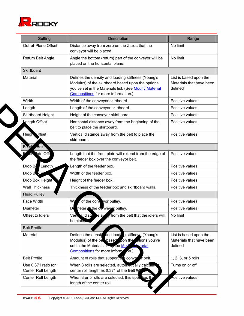
Page 66 Copyright © 2015, ESSS, GDI, and RDI. All Rights Reserved.
Setting Description Range
Out-of-Plane Offset Distance away from zero on the Z axis that the
conveyor will be placed.
No limit
Return Belt Angle Angle the bottom (return) part of the conveyor will be
placed on the horizontal plane.
No limit
Skirtboard
Material Defines the density and loading stiffness (Young’s
Modulus) of the skirtboard based upon the options
you’ve set in the Materials list. (See Modify Material
Compositions for more information.)
List is based upon the
Materials that have been
defined
Width Width of the conveyor skirtboard. Positive values
Length Length of the conveyor skirtboard. Positive values
Skirtboard Height Height of the conveyor skirtboard. Positive values
Length Offset Horizontal distance away from the beginning of the
belt to place the skirtboard.
Positive values
Height Offset Vertical distance away from the belt to place the
skirtboard.
Positive values
Feeder Box
Front Plate Offset Length that the front plate will extend from the edge of
the feeder box over the conveyor belt.
Positive values
Drop Box Length Length of the feeder box. Positive values
Drop Box Width Width of the feeder box. Positive values
Drop Box Height Height of the feeder box. Positive values
Wall Thickness Thickness of the feeder box and skirtboard walls. Positive values
Head Pulley
Face Width Width of the conveyor pulley. Positive values
Diameter Diameter of the conveyor pulley. Positive values
Offset to Idlers Vertical distance away from the belt that the idlers will
be placed.
No limit
Belt Profile
Material Defines the density and loading stiffness (Young’s
Modulus) of the belt based upon the options you’ve
set in the Materials list. (See Modify Material
Compositions for more information.)
List is based upon the
Materials that have been
defined
Belt Profile Amount of rolls that support the conveyor belt. 1, 2, 3, or 5 rolls
Use 0.371 ratio for
Center Roll Length
When 3 rolls are selected, automatically calculates
center roll length as 0.371 of the Belt Width.
Turns on or off
Center Roll Length When 3 or 5 rolls are selected, this specifies the
length of the center roll.
Positive values
安世
亚太
PERA Global

Copyright © 2015, ESSS, GDI, and RDI. All Rights Reserved. Page 67
Setting Description Range
Troughing Angle The degree by which the belt trough is formed
between the side and center rolls.
0>90
Lower Corner Radius Radius of the inside corner between the center and
side rolls. The bigger the value, the smoother the
transition.
Positive values
Side Roll Length When 5 rolls are selected, this specifies the length of
the two side rolls closest to the center roll.
Positive values
Use 0.223 ratio for Roll
Lengths
When 5 rolls are selected, automatically calculates the
side roll length as 0.223 of the Belt Width.
Turns on or off
Last Roll Angle When 5 rolls are selected, this specifies the degree by
which the belt trough is formed between the side and
outer rolls.
0<90
Upper Corner Radius When 5 rolls are selected, this specifies the radius of
the inside corner between the side and outer rolls. The
bigger the value, the smoother the transition.
Positive values
Belt Motion
Belt Speed Full speed of the conveyor belt after it completes the
Acceleration Period.
Positive values
Beginning Start Time The time you want the belt to begin moving. This is
when the Acceleration Period begins.
Positive values
Beginning Stop Time The time you want the belt to begin stopping. This is
when the Deceleration Period begins.
Positive values
Acceleration Period The length of time you want the belt to take to reach
full Belt Speed. Acceleration starts at the Beginning
Start Time and ends after the time period you specify
here.
Positive values
Deceleration Period The length of time you want the belt to take to come to
a full stop. Deceleration starts at the Beginning Stop
Time and ends after the time period you specify here.
Positive values
安世
亚太
PERA Global

Page 68 Copyright © 2015, ESSS, GDI, and RDI. All Rights Reserved.
Use the figures and table below to understand the various parameters you can set for a default inlet.
Figure 36: Default Inlet, Simulation Configuration parameters in the Data Editors panel
安世
亚太
PERA Global

Copyright © 2015, ESSS, GDI, and RDI. All Rights Reserved. Page 69
Figure 37: Default Inlet, Geometry parameters in the Data Editors panel
Table 15: Default Inlet parameter options (both tabs)
Setting Description Range
Name Enables you to specify a unique identifier for the geometry
component.
No limit
Simulation Configuration
Start Time The time you want particles to begin dropping from the inlet. Positive values
Stop Time The time you want particles to stop dropping from the inlet. Positive values
Stop All
Discharge at
Stop Time
In cases where the inlet delays particle release due to other
particles or boundaries being in the way, selecting this item
ensures that particles stop releasing at the Stop Time. If this
item is cleared, particles will stop releasing when the
originally calculated number of particles have been released.
Turns on or off
Use Periodic Inlet
Discharge
When selected, enables particles to be released from an inlet
in periodic bursts. When cleared, particles will be released in
a continuous flow.
Turns on or off
Period Amount of time between discharges. Positive values
Discharge Time Amount of time each period of discharge lasts. Positive values
Target Normal
Velocity
When selected, enables you to set the normal speed of the
particles being released from the inlet. The speed is
measured in local coordinates.
Positive values (but
limited by flow rate)
Ux-local Horizontal speed of the particles being released from the
inlet. Measured in local coordinates.
No limit
安世
亚太
PERA Global

Page 70 Copyright © 2015, ESSS, GDI, and RDI. All Rights Reserved.
Setting Description Range
Uz-local Out-of-plane speed of the particles being released from the
inlet. Measured in local coordinates.
No limit
Geometry
Type Determines the shape of the inlet. You can create
rectangular, circular, and donut-shaped inlets.
Rectangular; Circular
Center
Coordinates
Location of the inlet’s center point along the X, Y, and Z axes
respectively.
No limit
Alignment Angle The amount of rotation around the Y-axis. No limit
Length For rectangular inlets, the length of the inlet sides. No limit
Width For rectangular inlets, the width of the inlet. No limit
Incline Angle The amount of rotation with respect to the horizontal plane. No limit
Min. Radius Used for making donut- or ring-shaped inlets, this is the size
of the inlet's inner radius.
For donut- or ring-shaped inlets, make value > 0
(greater than zero).
For circular inlets, make value = 0 (equal to zero).
Positive values
Max. Radius For circular inlets, this is the size of the inlet's outer radius. Positive values
安世
亚太
PERA Global

Copyright © 2015, ESSS, GDI, and RDI. All Rights Reserved. Page 71
Use the following figures and table to understand the various parameters that you can set for a default
receiving conveyor.
Figure 38: Default Receiving Conveyor, Geometry parameters in the Data Editors panel
Figure 39: Default Receiving Conveyor, Orientation parameters in the Data Editors panel
安世
亚太
PERA Global

Page 72 Copyright © 2015, ESSS, GDI, and RDI. All Rights Reserved.
Figure 40: Default Receiving Conveyor, Skirtboard parameters in the Data Editors panel
Figure 41: Default Receiving Conveyor, Belt Profile parameters in the Data Editors panel
安世
亚太
PERA Global

Copyright © 2015, ESSS, GDI, and RDI. All Rights Reserved. Page 73
Figure 42: Default Receiving Conveyor, Belt Motion parameters in the Data Editors panel
Table 16: Default Receiving Conveyor parameter options (all tabs)
Setting Description Range
Name Enables you to specify a unique identifier for the
geometry component.
No limit
Geometry
Length Length of the conveyor belt. Positive values
Belt Width Width of the conveyor belt. Positive values
Triangle Size Size of the triangular components into which the
boundary is divided. In general, the smaller the
Triangle Size, the more accurate the wear
calculations.
Positive values
Belt Thickness Thickness of the conveyor belt. Affects visualization
only; does not affect calculations.
Positive values
Orientation
Alignment Angle Angle the top (carry) part of the conveyor will be
placed on the horizontal plane.
No limit
Belt Incline Angle Angle the conveyor will be placed on the vertical
plane.
No limit
Vertical Offset Distance away from zero on the Y axis that the
conveyor will be placed.
No limit
Horizontal Offset Distance away from zero on the X axis that the
conveyor will be placed.
No limit
Out-of-Plane Offset Distance away from zero on the Z axis that the
conveyor will be placed.
No limit
Skirtboard
安世
亚太
PERA Global

Page 74 Copyright © 2015, ESSS, GDI, and RDI. All Rights Reserved.
Setting Description Range
Material Defines the density and loading stiffness (Young’s
Modulus) of the skirtboard based upon the options
you’ve set in the Materials list. (See Modify Material
Compositions for more information.)
List is based upon the
Materials that have been
defined
Width Width of the conveyor skirtboard. Positive values
Length Length of the conveyor skirtboard. Positive values
Skirtboard Height Height of the conveyor skirtboard. Positive values
Length Offset Horizontal distance away from the beginning of the
belt to place the skirtboard.
Positive values
Height Offset Vertical distance away from the belt to place the
skirtboard.
Positive values
Belt Profile
Material Defines the density and loading stiffness (Young’s
Modulus) of the belt based upon the options you’ve
set in the Materials list. (See Modify Material
Compositions for more information.)
List is based upon the
Materials that have been
defined
Belt Profile Amount of rolls that support the conveyor belt. 1, 2, 3, or 5 rolls
Use 0.371 ratio for
Center Roll Length
When 3 rolls are selected, automatically calculates
center roll length as 0.371 of the Belt Width.
Turns on or off
Center Roll Length When 3 or 5 rolls are selected, this specifies the
length of the center roll.
Positive values
Troughing Angle The degree by which the belt trough is formed
between the side and center rolls.
0>90
Lower Corner Radius Radius of the inside corner between the center and
side rolls. The bigger the value, the smoother the
transition.
Positive values
Side Roll Length When 5 rolls are selected, this specifies the length of
the two side rolls closest to the center roll.
Positive values
Use 0.223 ratio for Roll
Lengths
When 5 rolls are selected, automatically calculates the
side roll length as 0.223 of the Belt Width.
Turns on or off
Last Roll Angle When 5 rolls are selected, this specifies the degree by
which the belt trough is formed between the side and
outer rolls.
0<90
Upper Corner Radius When 5 rolls are selected, this specifies the radius of
the inside corner between the side and outer rolls. The
bigger the value, the smoother the transition.
Positive values
Belt Motion
Belt Speed Full speed of the conveyor belt after it completes the
Acceleration Period.
Positive values
安世
亚太
PERA Global

Copyright © 2015, ESSS, GDI, and RDI. All Rights Reserved. Page 75
Setting Description Range
Beginning Start Time The time you want the belt to begin moving. This is
when the Acceleration Period begins.
Positive values
Beginning Stop Time The time you want the belt to begin stopping. This is
when the Deceleration Period begins.
Positive values
Acceleration Period The length of time you want the belt to take to reach
full Belt Speed. Acceleration starts at the Beginning
Start Time and ends after the time period you specify
here.
Positive values
Deceleration Period The length of time you want the belt to take to come to
a full stop. Deceleration starts at the Beginning Stop
Time and ends after the time period you specify here.
Positive values
安世
亚太
PERA Global

Page 76 Copyright © 2015, ESSS, GDI, and RDI. All Rights Reserved.
Use the following figures and table to understand the various parameters that you can set for an imported
(custom) geometry.
Figure 43: Imported (custom) geometry, Geometry parameters in the Data Editors panel
安世
亚太
PERA Global

Copyright © 2015, ESSS, GDI, and RDI. All Rights Reserved. Page 77
Figure 44: Imported (custom) geometry, Mass parameters in the Data Editors panel
Figure 45: Imported (custom) geometry, Wear parameters in the Data Editors panel
安世
亚太
PERA Global
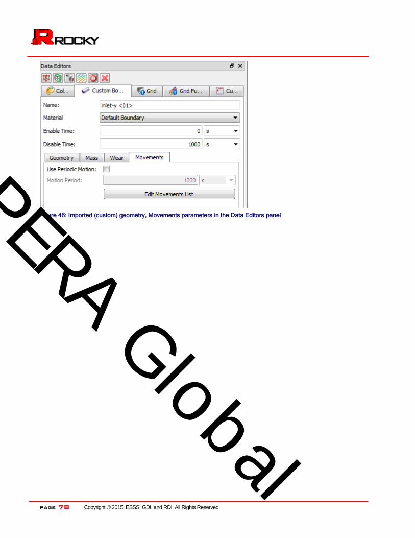
Page 78 Copyright © 2015, ESSS, GDI, and RDI. All Rights Reserved.
Figure 46: Imported (custom) geometry, Movements parameters in the Data Editors panel
安世
亚太
PERA Global

Copyright © 2015, ESSS, GDI, and RDI. All Rights Reserved. Page 79
Figure 47: Custom Movements dialog, Rotation and Translation parameters. (Same parameters as Rotation and
Translation Without Displacement.)
Figure 48: Custom Movements dialog, Vibration parameters
安世
亚太
PERA Global

Page 80 Copyright © 2015, ESSS, GDI, and RDI. All Rights Reserved.
Figure 49: Custom Movements dialog, Pendulum parameters
Table 17: Imported (custom) geometry parameter options (all available)
Setting Description Range
Name Enables you to specify a unique identifier for the geometry
component.
Not editable
Material Defines the density and loading stiffness (Young’s Modulus) of
the skirtboard based upon the options you’ve set in the
Materials list. (See Modify Material Composition for more
information.)
List is based upon the
Materials that have been
defined
Enable Time The time you want the geometry to appear in the simulation.
Tip: To have the geometry appear at simulation onset, keep
Enable Time as zero (0).
Positive values
Disable Time The time you want the geometry to disappear from the
simulation.
Tip: To have the geometry stay for the duration of the
simulation, keep Disable Time as 1000 s or the maximum
length of your simulation.
Positive values
Geometry
Number of
Triangles
Number of boundary triangles imported from the STL, XGL,
DXF 3D faces, CAS, or MSH file.
Not editable
Triangle Size Size of the individual triangular components into which the
geometry is divided. In general, the smaller the triangles, the
more accurate the wear calculations.
Positive values
Offset, Horizontal Distance away from the imported X-axis’ coordinate value.
This does not create moving geometries; rather this re-locates
the original geometry position.
No limit
Offset, Vertical Distance away from the imported Y-axis’ coordinate value.
This does not create moving geometries; rather this re-locates
the original geometry position.
No limit
安世
亚太
PERA Global

Copyright © 2015, ESSS, GDI, and RDI. All Rights Reserved. Page 81
Setting Description Range
Offset, Out-of-
Plane
Distance away from the imported Z-axis’ coordinate value.
This does not create moving geometries; rather this re-locates
the original geometry position.
No limit
Mass
Boundary Mass When Rotation and Translation and Free Motion are selected
in the Movements List, this is the mass of the geometry.
Positive values
Moments of Inertia When Rotation and Translation and Free Motion are selected
in the Movements List, these are the principal moments of
inertia along each of the 3 axes. It is assumed that the axes
coincide with the x, y, and z axes at the start of the simulation.
Positive values
Wear
Use Wear Enables the surface of the geometry to appear modified over
time as it gets worn down by particle interaction.
Turns on or off
Wear Law The calculation used to perform wear modifications of the
geometry surface. For this release, only Shear Work
Proportionality is enabled. This means that the volume of
geometry removed is proportional to the shear wear applied to
the geometry.
Note: You cannot use this type of wear modification if the
geometry has movements set up as translation/rotation
without displacement.
Shear Work
Proportionality
Volume/Shear
Work Ratio
The amount of surface volume that is removed per shear work
applied.
Note: This is a calibration step that comes from real-world
wear data you have collected using similar types of liners.
Positive values
Movements
Use Periodic
Motion
Enables a motion period to be repeated or looped throughout
the simulation.
(See also To enable geometry movements to be repeated.)
Turns on or off
Motion Period When Periodic Motion is selected, enables you to enter the
amount of time for which movement is repeated or looped
throughout the simulation.
Tips:
Entering the exact time amount for which you have
specified movement(s) will result in a seamless repeat
of all movements.
Entering a smaller time amount will result in the latter
part of your movement not occurring.
Entering a larger time amount will result in no
movement at the end of each period.
Positive values
安世
亚太
PERA Global

Page 82 Copyright © 2015, ESSS, GDI, and RDI. All Rights Reserved.
Setting Description Range
Custom Movements (from the Movements tab, click Edit Movements List)
Start Movement
Time
The time you want geometry movement to begin. Positive values
Stop Movement
Time
The time you want geometry movement to stop. Positive values
Movement Type Used to create moving geometries and vibration.
In general, choose:
Rotation and Translation when you want the geometry
to move physically from one location to another. For
example, a gate that rises or a mill that rotates.
Rotation and Translation without Displacement when
you want the geometry to stay stationary but still have
surface velocity applied. For example, a stationary
conveyor whose belt moves particles.
Vibration when you want the geometry to oscillate. For
example, a vibrating pan feeder.
Pendulum when you want the geometry to swing back
and forth along a center point, like a pendulum.
Notes:
Translation/Rotation without Displacement is how all
default feed and receiving conveyors in Rocky are set
up.
The values are set up in the local coordinates system
at the beginning of the time period. At zero time, this
system coincides with the global system.
Any gaps in the movement time periods will be treated
as no motion (Movement Type=None).
(See also Enable Moving, Rotating, Vibrating, or Swinging
Geometries.)
None;
Rotation and
Translation;
Rotation and Translation
without Displacement;
Vibration;
Pendulum
Motion
Coordinates
Defines which coordinate system the movement values are
based on:
Local: Coordinate system is relative to the position of
the geometry.
Global: Coordinate system is relative to the simulation
in general.
Note: Most movement settings can be either Local or Global
but Center of Rotation values can only be Local.
Local;
Global
Translation Parameters
安世
亚太
PERA Global

Copyright © 2015, ESSS, GDI, and RDI. All Rights Reserved. Page 83
Setting Description Range
Free Motion When Rotation and Translation is selected, this enables the
geometry to move freely along the chosen Axis under gravity
and particle forces.
Notes:
Free movement is affected by particle placement,
Boundary Mass, and Force.
The amount of movement is restricted by Minimum
Displacement and Maximum Displacement.
Free Movement cannot be specified for Rotation and
Translation Without Movement.
Turns on or off
Force When Free Motion is selected, this enables an external force
to be applied to the geometry. For example, the added force of
a car pressing down on a wheel.
Positive values
Velocity This is the translational velocity along the axis. No limit
Acceleration This is the linear acceleration along the axis. No limit
Minimum
Displacement
When Free Motion is selected, this is the minimum
displacement length that the geometry is allowed to freely
move.
Positive values
Maximum
Displacement
When Free Motion is selected, this is the maximum
displacement length that the geometry is allowed to freely
move.
Positive values
Rotation Parameters
Specify Gravity
Center (local)
If Free Motion is selected, selecting this option enables you to
use the Gravity Center values to specify the coordinates of the
center point of gravity. If this option is not selected, center of
gravity is assumed to be the same as the center of rotation for
the geometry.
Note: Even if the Global coordinate system is selected, this
value will be set within the Local coordinate system.
Turns on or off
Free Motion When Rotation and Translation is selected, this enables the
boundary to rotate freely around the chosen Direction and
under the particles' torque. Free motion is affected by particle
placement, Torque, and Moments of Inertia.
Turns on or off
Torque When Free Motion is selected, this enables an external torque
to be applied to the geometry.
No limit
Velocity This is the rotational velocity along the axis. No limit
Acceleration This is the angular acceleration along the axis. No limit
安世
亚太
PERA Global

Page 84 Copyright © 2015, ESSS, GDI, and RDI. All Rights Reserved.
Setting Description Range
Center This is the location in coordinates of the center point of
rotation.
Note: Even if the Global coordinate system is selected, this
value will be set within the Local coordinate system.
No limit
Gravity Center If both the Free Motion and Specify Gravity Center (local)
options are selected, then this is the location in coordinates of
the center point of gravity for the geometry.
No limit
Vibration Parameters
Frequency When Vibration is selected, this determines how frequently the
oscillation of the geometry occurs.
Positive values
First Axis
Direction Determines the direction of the first elliptical axis by setting the
coordinate values of a direction vector of length 1.
No limit but values
entered will be
normalized to equal a
length of 1
Amplitude Height of the oscillation curve along the first axis. Lower
values produce minor vibration; higher values produce
significant vibration.
Positive values
Second Axis
Direction Determines the direction of the second elliptical axis by setting
the coordinate values of a direction vector of length 1.
No limit but values
entered will be
normalized to equal a
length of 1 and adjusted
to be perpendicular to
first axis
Amplitude Height of the oscillation curve along the second axis. Lower
values produce minor vibration; higher values produce
significant vibration.
Positive values
Pendulum Parameters
Frequency When Pendulum is selected, this determines how frequently
the swinging of the geometry occurs.
No limit
Amplitude Height (in degrees) of the swing's arch. Positive values
Plane The 2-D plane upon which the swinging will occur. XY, YZ, ZX
Pivot Point Location in coordinates of the point upon which the geometry
will swing.
Note: Even if the Global coordinate system is selected, this
value will be set within the Local coordinate system.
No limit
安世
亚太
PERA Global

Copyright © 2015, ESSS, GDI, and RDI. All Rights Reserved. Page 85
To edit the parameters for geometry:
1. From the Data panel, under Geometries, select the name of the geometry that you want to edit.
The parameters for that geometry are displayed in the Data Editors panel. The tab named with the type
of geometry you selected (for example, “Custom Boundary”, “Feed Conveyor”, and so on) will be active.
2. From the Data Editors panel, enter the information you want on the active tab, being sure to select each
of the various sub-tabs or dialogs that contain parameters you want to modify.
Tip: To set the same value for a parameter across multiple similar geometries, multi-select the geometries
you want in the Data panel (SHIFT + left-click for a continuous group; CTRL + left-click for discontinuous
items) and then change the values you want in the Data Editor panel. Only those parameters common across
all selected geometries will be editable but any changes made will populate across the selected group.
To remove a geometry
From the Data panel, under Geometries, right-click the name of the geometry you want to remove,
and then click Remove Geometry.
Modify Material Compositions
Rocky enables you to specify unique densities and loading stiffnesses (Young’s Modulus) for the conveyor
belts, geometries, and particle sets used in your simulation. This helps you ensure that the various materials
being simulated interact with each other in as realistic a way as possible.
By default, Rocky defines three Material sets for each simulation, including one each for Default Belt, Default
Boundary, and Default Particle. While you can modify the settings for these default Materials and also add
additional Material definitions if you choose, you cannot remove these default Materials from the simulation.
Materials you define here will be used when defining the parameters for Geometries, Particles, and Materials
Interactions.
Use the figures and table below to help you understand the various parameters you can modify for Materials.
安世
亚太
PERA Global

Page 86 Copyright © 2015, ESSS, GDI, and RDI. All Rights Reserved.
Figure 50: Material parameters in the Data Editors panel
Figure 51: Default Material parameters in the Data Editors panel
安世
亚太
PERA Global

Copyright © 2015, ESSS, GDI, and RDI. All Rights Reserved. Page 87
Table 18: Material parameter options (all available)
Setting Description Range
Bulk Solid Fraction for
Materials
For all Materials that have Use Bulk Density
selected, this number is applied to the Density
value.
Notes:
This value applies to all Materials in the
simulation.
One minus this value is the void ratio of
the Materials. (The default void ratio is
0.4.)
0<1
Name Enables you to specify a unique identifier for the
Material.
99 character limit
Density Density of the Material. How it is used is
affected by the Use Bulk Density setting.
Positive values
Young’s Modulus Formerly “Loading Stiffness”, this value defines
how rigidly the Material will interact with another
Material. In general, the higher the value, the
more accurate the results but the longer the
processing time. This value roughly equals
Young’s material bulk elastic modulus.
Positive values
Use Bulk Density When selected, Density will be divided by Bulk
Solid Fraction for Materials to determine
Material density. When cleared, only the Density
value will be used.
Turns on or off
To modify parameters for an existing or default Material
1. From the Data panel do one of the following:
To modify the Bulk Solid Fraction for Materials value for all Materials in the simulation, select
Materials.
To modify an individual Material’s parameters, under Materials, select the name of the Material you
want to modify.
The parameters for the Material you selected are displayed in the Data Editors panel.
2. From the Data Editors panel, modify the parameters as you want.
To add a new Material
From the Data panel, right-click Materials and then click Create Material.
The new Material appears in the Materials list in alphabetical (case-sensitive) order.
安世
亚太
PERA Global

Page 88 Copyright © 2015, ESSS, GDI, and RDI. All Rights Reserved.
To remove a (non-default) Material you have added
Note: You can remove only those Materials that you have added. The three default Materials Rocky
automatically includes in your simulation are not removable.
From the Data panel, under Materials, right click the name of the Material you want to remove, and
then click Remove Material.
Modify Material Interaction and Adhesion Values
Rocky enables you to specify unique frictions and adhesion values for each Material-to-Material combination
that exists in your simulation, including the interaction of a Material to itself, and also to each other Material
defined in the Materials list.
Modifying these values enables you to calibrate how “wet” or “sticky” a Material acts when it comes into
contact with another Material, enabling you to create simulations that more closely mirror real-world
conditions.
Note: Even though Rocky enables you to set interactions of geometries to other geometries, these types of
interactions have no value to your simulation. The only values that will affect your simulation are those
interactions between particles (particle-to-particle) or between particles and boundaries (particle-to-
geometry).
Use the figures and table below to help you understand the various parameters you can modify for Materials
Interaction.
安世
亚太
PERA Global

Copyright © 2015, ESSS, GDI, and RDI. All Rights Reserved. Page 89
Figure 52: Materials Interaction parameters in the Data Editors panel
Table 19: Materials Interaction parameter options
Setting Description Range
Adhesion Model Defines how adhesion between materials are
calculated:
Linear: Adhesive force increases
linearly with the distance between
Materials. Uses Stiffness fraction value.
Constant: Adhesive force stays constant
no matter the distance between
Materials. This is the same model that
was used in version 2 of Rocky.
Linear; Constant
Static Friction Maximum ratio of contact tangential force to
normal force before onset of sliding.
Positive values (see also
Best Practices for Setting Up
Particles)
Dynamic Friction Maximum ratio of contact tangential force to
normal force after onset of sliding.
Positive values; usually less
than Static Friction (see also
Best Practices for Setting Up
Particles)
安世
亚太
PERA Global

Page 90 Copyright © 2015, ESSS, GDI, and RDI. All Rights Reserved.
Setting Description Range
Coefficient of
Restitution
Measure of energy dissipation. 0.1 - 1
Adhesive Distance The distance between the two Materials before
forces are applied.
Positive values
Force fraction When a Constant Adhesion Model is chosen,
this is the ratio of the adhesive force on the first
Material to the gravity force of the second
Material.
Positive values
Stiffness fraction When a Linear Adhesion Model is chosen, this
is the ratio of adhesive stiffness to the loading
elastic stiffness of the contact between the two
materials.
0-1
To modify the interaction or adhesion values for a Material-to-Material set
1. From the Data panel, select Materials Interaction.
The Materials Interaction parameters become active in the Data Editors panel.
2. From the Data Editors panel, select what you want for Adhesion Model, and then do all of the following:
a. From Select Material list on the left, select the first Material in the Material-to-Material combination for
which you want to modify adhesion values.
b. From the Select Materials list on the right, select the next Material in the Material-to-Material
combination for which you want to modify adhesion values.
The parameters that define the interaction between the two Materials you selected appear in the
Data Editors panel.
c. Modify the values as you want.
d. Repeat steps 2a-2c for each of the Material-to-Material combinations you want to modify.
Add and Edit Particle Groups
A particle group is created when you specify the shape of a particular particle, and then choose the size
ranges you want replicated in your simulation. You can add as many particle groups containing as many as
size ranges each to a given simulation as you like, but you must have added at least one particle group to
process a simulation.
Use the figure and table below to help you understand the various parameters you can set for each Particle
group.
安世
亚太
PERA Global

Copyright © 2015, ESSS, GDI, and RDI. All Rights Reserved. Page 91
Figure 53: Particle, Size Distribution parameters in the Data Editors panel
安世
亚太
PERA Global

Page 92 Copyright © 2015, ESSS, GDI, and RDI. All Rights Reserved.
Figure 54: Particle, Geometry parameters in the Data Editors panel
Figure 55: Particle, Breakage parameters in the Data Editors panel
安世
亚太
PERA Global

Copyright © 2015, ESSS, GDI, and RDI. All Rights Reserved. Page 93
Table 20: Particle parameter options (all tabs)
Setting Description Range
Name Enables you to specify a unique identifier for the particular particle
group.
99 character limit
Material Defines the density and loading stiffness (Young’s Modulus) of the
Particle group based upon the options you’ve defined in the Materials
list. (See Modify Material Composition for more information.)
List is based upon
the Materials that
have been defined
Size Distribution
Size Type Determines how the size of the particle will be measured.
Sieve: Particle size will be based upon the dimensions of a
square hole just big enough for the particle to pass through.
This use of virtual “mesh” determines the size of the particles
no matter what shape they are.
Equivalent Diameter: Particle size of irregularly-shaped
objects will be based upon the diameter of a sphere of
equivalent volume.
Sieve; Equivalent
Diameter
Size The dimension of the particle based upon the Size Type value that is
set.
If only one size is specified for a particle group, only particles of that
size will be used during the simulation. This is because the smallest
Size value specified will always have no range.
If more than one size is specified for a particle group, a range of sizes
within the Size parameter will be used for each Cumulative %
provided. The one exception is for the smallest Size value, which will
have no range.
For example, for the sizes and percentages specified below:
20% (100-80) of the particles will be in various sizes between
0.05 and 0.1 meters.
60% (80-20) of the particles will be in various sizes between
0.01 and.0.05 meters.
The rest of the particles (20%) will be exactly 0.01 meters in
size (no range).
Positive values;
sizes should
decrease as you
go down the Size
Distribution table
安世
亚太
PERA Global
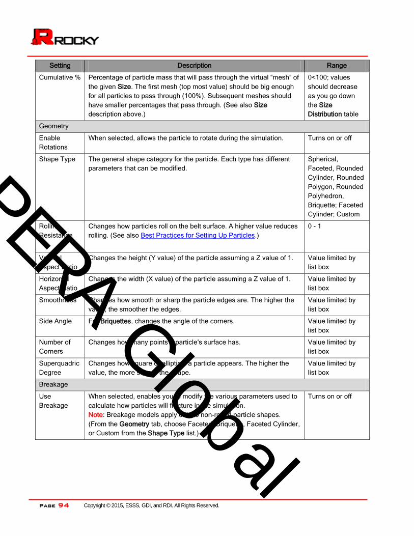
Page 94 Copyright © 2015, ESSS, GDI, and RDI. All Rights Reserved.
Setting Description Range
Cumulative % Percentage of particle mass that will pass through the virtual “mesh” of
the given Size. The first mesh (top most value) should be big enough
for all particles to pass through (100%). Subsequent meshes should
have smaller percentages that pass through. (See also Size
description above.)
0<100; values
should decrease
as you go down
the Size
Distribution table
Geometry
Enable
Rotations
When selected, allows the particle to rotate during the simulation. Turns on or off
Shape Type The general shape category for the particle. Each type has different
parameters that can be modified.
Spherical,
Faceted, Rounded
Cylinder, Rounded
Polygon, Rounded
Polyhedron,
Briquette; Faceted
Cylinder; Custom
Rolling
Resistance
Changes how particles roll on the belt surface. A higher value reduces
rolling. (See also Best Practices for Setting Up Particles.)
0 - 1
Vertical
Aspect Ratio
Changes the height (Y value) of the particle assuming a Z value of 1. Value limited by
list box
Horizontal
Aspect Ratio
Changes the width (X value) of the particle assuming a Z value of 1. Value limited by
list box
Smoothness Changes how smooth or sharp the particle edges are. The higher the
value, the smoother the edges.
Value limited by
list box
Side Angle For Briquettes, changes the angle of the corners. Value limited by
list box
Number of
Corners
Changes how many points a particle's surface has. Value limited by
list box
Superquadric
Degree
Changes how square or elliptical a particle appears. The higher the
value, the more square the shape.
Value limited by
list box
Breakage
Use
Breakage
When selected, enables you to modify the various parameters used to
calculate how particles will fracture in the simulation.
Note: Breakage models apply only to non-round particle shapes.
(From the Geometry tab, choose Faceted, Briquette, Faceted Cylinder,
or Custom from the Shape Type list.)
Turns on or off
安世
亚太
PERA Global

Copyright © 2015, ESSS, GDI, and RDI. All Rights Reserved. Page 95
Setting Description Range
Model Name of the model that Rocky uses to calculate fracturing.
For more information about the breakage model used in Rocky, refer
to the 2013 paper by Alex Potapov et al: Computer Simulation of Coal
Breakage in Conveyor Transfer Chutes with Rocky Discrete Element
Method Package.
Exp-T10
Distribution Type of fragment distribution size used in the model. Gaudin-Schumann
Minimum
Size
Smallest size the particle fragments can be after breaking. Any value
Reference
Size
Lref in the model equation. Any value
Minimum
Specific
Energy
If the total specific energy for a particle that comes into contact with
another particle or geometry is less than this value, breakage will not
occur.
emin in the model equation.
Any value
Selection
Function
Coefficient
The particle breakage strength parameter, which is a material
constant.
S in the model equation.
Any value
Maximum
T10 Value
Maximum degree of impact breakage,
M in the model equation.
Value limited by
list box
To add a new Particle group
From the Data panel, right-click Particles, and then click Create Particle.
A new Particle is listed under Particles in alphabetical (case-sensitive) order.
To modify the parameters of a Particle group
1. From the Data panel, under Particles, click the name of the Particle group you want to modify.
The parameters for the Particle become active in the Data Editors panel.
2. From the Data Editors panel, modify the parameters as you want.
To remove an existing Particle group
From the Data panel, under Particles, right-click the name of the Particle group you want to remove,
and then click Remove Particle.
Add and Edit Particle Inputs
The Inputs section on the Data panel is where you specify where the various particle groups will be entering
your simulation. Particles can enter simulations through the Feed Conveyor geometry, or through any Inlets
that you have created.
安世
亚太
PERA Global

Page 96 Copyright © 2015, ESSS, GDI, and RDI. All Rights Reserved.
You can specify as many particle inputs as you like. But before you can process your simulation, you must
create at least one Particle Input and provide the Tonnage value for at least one particle group.
Use the figure and table below to help you understand the various parameters you can set for particle inputs.
Figure 56: Particle Input, Data Editors panel
Table 21: Particle Input parameter options
Setting Description Range
Name Enables you to specify a unique identifier for the particle
input.
99 character limit
Entry Point The Feed Conveyor or inlet from which the particles are
released during the simulation.
Any Feed Conveyor or Inlet that
has been included in the
simulation
Particle The particle group that you want to enter the simulation
from the Entry Point specified.
Any particle group specified in
the simulation
Tonnage The mass flow rate for the particle group that you want
released from this entry point per hour.
Positive values
安世
亚太
PERA Global

Copyright © 2015, ESSS, GDI, and RDI. All Rights Reserved. Page 97
To create a new Input
1. From the Data panel, click Input, and the from the Data Editors panel, click the Create Particle Input
button.
A new Particle Input component appears under Input in the Data panel.
2. From the Data panel, click the Particle Input you just added and then from the Data Editors panel, enter
the Name and set the Entry Point you want.
3. Under Entry Point, click the Add button.
A new row appears at the bottom of the table.
4. Under Particle, choose the particle group that you want and then under Tonnage, specify what mass flow
rate you want associated with it.
5. Repeat steps 3-4 for each particle group that you want entering the simulation from the Entry Point
specified.
Tips:
To insert a new row beneath the selected row, click the Insert button.
To remove the selected row, click the Remove button.
To remove all rows in the table, click the Remove All button.
To edit an Input
From the Data panel, click the Particle Input you want to edit, and then from the Data Editors panel,
modify the settings as desired.
To remove an Input
From the Data panel, click the Particle Input you want to remove, and then from the Data Editors
panel, click the Remove button.
Set or Modify Air Flow Properties
In Rocky, air flow is a CFD Coupling option that represents the way gas and dust-like particles interact with
the flow of material in your chute, mill, or other materials handling design. During set up, you can turn on air
flow properties; change the density, viscosity, and size of the air flow cells; and set air flow coordinate limits.
Use the figures and table below to understand the various parameters you can set for air flow.
安世
亚太
PERA Global

Page 98 Copyright © 2015, ESSS, GDI, and RDI. All Rights Reserved.
Figure 57: CFD Coupling, Air Flow in Data Editors panel
Table 22: Air Flow Settings
Setting Description Range
Use Air Flow Enables air flow calculations to be included in the
simulation.
Turns on or off
Start When Particles
Enter
Enables air flow calculations to start as soon as
particles appear in the air flow limit box.
Turns on or off
Air Density The density of the air. Positive values
Air Viscosity The viscosity of the air. Positive values
Cell Size The size of an air flow cell. Positive values
安世
亚太
PERA Global

Copyright © 2015, ESSS, GDI, and RDI. All Rights Reserved. Page 99
Setting Description Range
Interaction Scale Determines the interaction between the particle and
the air.
Positive values.
(It is recommended that the
default value of 0.25 is
used.)
Start Time When Start When Particles Enter is cleared, this is
the time that air flow calculations begin during the
simulation.
Positive values
Speed of Sound The speed of sound, which is used to calculate air
flow.
Positive values
Boundary Conditions
First Derivative This order provides more stability to the calculations
but less accuracy.
Turns off or on
Second Derivative This order provides more accuracy to the calculations
but less stability.
Turns off or on
Coordinate Limits
X Min/Max Distance away from zero on the X axis to place the
nearest and farthest corner of the air flow limit box.
No limit
Y Min/Max Distance away from zero on the Y axis to place the
nearest and farthest corners of the air flow limit box.
No limit
Z Min/Max Distance away from zero on the Z axis to place the
nearest and farthest corners of the air flow limit box.
No limit
To turn on air flow properties for a simulation
1. From the Data panel, click CFD Coupling and then from the Data Editors panel, choose Air Flow from the
Coupling Mode list.
The Air Flow component appears in the Data panel beneath CFD Coupling.
2. In the Data panel, click the new Air Flow component.
3. From the Data Editors panel, on the Air Flow tab, ensure the Use Air Flow checkbox is enabled, and then
modify the settings as you want.
To modify air flow properties
1. From the Data panel, under CFD Coupling, click Air Flow.
2. From the Data Editors panel, on the Air Flow tab, modify the settings as you want.
To turn off airflow properties
1. From the Data panel, under CFD Coupling, click Air Flow.
2. From the Data Editors panel, on the Air Flow tab, clear the Use Air Flow check box.
安世
亚太
PERA Global

Page 100 Copyright © 2015, ESSS, GDI, and RDI. All Rights Reserved.
Note: You can also remove Air Flow from your set up completely by choosing No Coupling from the Coupling
Mode list. (From the Data panel, click CFD Coupling and then from the Data Editors panel, make your
selection on the CFD Coupling tab.)
Verify Simulation Size
Before you process a simulation, it is a good idea to check the Simulation Summary dialog to get a rough
estimate of the simulation size. Taking this step can help you catch data entry errors, which has the potential
of saving you time in processing your simulation.
In general, the higher the values given on the Simulation Summary dialog, the longer the simulation will take
to process. (See also Best Practices for Faster Processing.)
Use the figure and table below to understand the various types of summary information provided for
simulations.
Table 23: Simulation Summary
Item Description
Number of Particles Total number of particles that will appear in the simulation, from start
to finish. The number is calculated based on particle shape, flow rate,
tonnage, and density values, as well as simulation time.
Number of Enabled Air Nodes When airflow is turned on, this is the number of air nodes that will be
used during the simulation. The number is calculated based on airflow
cell size and airflow boundary limits.
Number of Triangles Total number of geometry triangles that will be used in the simulation.
The number is calculated based on the Triangle Size value specified
in the various conveyor settings dialogs (Receiving Conveyor
Settings, Feed Conveyor Settings, and Custom Boundary Settings).
安世
亚太
PERA Global

Copyright © 2015, ESSS, GDI, and RDI. All Rights Reserved. Page 101
Item Description
Timestep Duration Number of individual calculations Rocky completes for each particle
every one second of simulation time. Timestep is an automatic and
dynamic value Rocky defines using particle size, density, contact
loading stiffness (Young’s Modulus), and restitution coefficients. For
example, if the time step is 1e-5, for every second of simulated real
time 100,000 calculations of forces, positions, and so on will be done
on every particle.
Note: This number will change based upon simulation parameters.
Domain minimum The coordinates of the nearest points geometry triangles are drawn. If
Set as Boundary Limits is selected, once a particle reaches these
limits, it will be removed from the calculation and, unless periodic
boundaries are selected, will disappear from the Display Area. (This is
done to save on processing power.) (See also Set Simulation-Wide
Parameters.)
Domain maximum The coordinates of the farthest points geometry triangles are drawn. If
Set as Boundary Limits is selected, once a particle reaches these
limits, it will be removed from the calculation and, unless periodic
boundaries are selected, will disappear from the Display Area. (This is
done to save on processing power.) (See also Set Simulation-Wide
Parameters.)
To verify the simulation size
1. Ensure that you have set up the minimum requirements for processing. (See also 3. Setting Up a
Simulation.)
2. From the Data panel, select Solver and then from the Data Editors panel, click Start Simulation.
3. On the Simulation Summary dialog, review the information provided and then do one of the following:
To return to setting up your simulation, click Cancel.
To start processing your simulation, click OK.
安世
亚太
PERA Global

Page 102 Copyright © 2015, ESSS, GDI, and RDI. All Rights Reserved.
4. Processing a Simulation
After you have set up your simulation (see 3. Setting Up a Simulation), you are ready to process it.
Processing is the step in which Rocky calculates at each progressive timestep how each individual particle
interacts with every other particle and boundary it comes into contact with.
The time it takes for your simulation to complete will depend upon the complication of the parameters you
have set, and the number and type of the processors you have chosen. Based upon these characteristics,
your simulation can take anywhere from a few minutes to several days to complete. (See also
Best Practices for Faster Processing.)
IMPORTANT: You are only able to set and change parameters during simulation setup so ensure that your
settings are correct before processing.
While your simulation is processing, you might stop and restart the simulation several times before your
simulation is complete. As the simulation is processing, you can see the progress in a 3D View window or
see data collect in a plot or histogram.
What would you like to do?
Start a Simulation
Stop a Simulation
Process Multiple Simulations at Once
Start a Simulation
You start a simulation either after you have finished setting simulation parameters and are ready to begin the
calculations, or have stopped a simulation and want to continue processing it. In this step, you select whether
you want CPU or GPU processing, the number of processors, and which direction you want parallel slicing to
occur.
While the simulation is processing, you are able to use Rocky to review your simulation settings, create
charts, graphs, and 3D Views of the data collected thus far, and more.
The only task you are unable to do while a simulation is processing is change the set up parameters. Doing
this would affect the calculations that Rocky is solving. To change the setup parameters, first stop the
simulation, change your parameters, and then start your simulation over from the beginning.
Use the image and table below to understand the parameters you can set for processing your simulation.
安世
亚太
PERA Global

Copyright © 2015, ESSS, GDI, and RDI. All Rights Reserved. Page 103
Figure 58: Solver, General Settings parameters in the Data Editors panel
Table 24: Processing Area
Setting Description Range
Simulation
Target
Enables you to select what portion of your computer will be doing the
processing.
CPU; GPU
Number of
Processors
Sets the number of computer processors (threads) the simulation will
use. In general, the more processors used, the faster the simulation
will complete.
It is recommended that you set this number equal to the amount of
cores available, or double the amount of cores if hyper-threading is
used.
Notes:
Setting more processors than what you have available will
slow the simulation.
Windows limits the number of processors to 64 so if you are
running Rocky on Windows, it is best to set this value to 64 or
less.
Positive values
Note: We covered these first
two options in the Set
Simulation-Wide
Parameters section.
安世
亚太
PERA Global

Page 104 Copyright © 2015, ESSS, GDI, and RDI. All Rights Reserved.
Parallel
Slicing
Sets the direction parallel slicing is made during processing. In
general, choose the direction that represents the longest boundary
component in your simulation. For example, if your longest boundary is
a conveyor oriented along the X-axis, choose X-Parallel Slicing. This
setting can help reduce processing time.
X-Parallel Slicing
Y-Parallel Slicing
Z-Parallel Slicing
To start processing a simulation from the beginning
1. From the Data panel, click Solver and then from the Data Editors panel, ensure the Solver | General
Settings tab is active.
2. Enter what you want for the Simulation Target, Number of Processors, and Slicing Direction options.
3. Click Start Simulation.
The Simulation Summary dialog appears.
4. Review the information in the Simulation Summary dialog, and then click OK. (For more information
about this dialog, see Verify Simulation Size.)
The simulation progress bar appears at the bottom of the screen and processing begins at the zero
Timestep. (See also Refer to the Rocky Title Bar for Simulation Progress Details.) When processing is
complete, the progress bar disappears.
Tips:
To see the progress of your simulation in a 3D View window, on the Solver tab, click Refresh Results
and then use the Play Simulation button on the Timestep toolbar.
To always see the latest results, select the Auto Refresh check box on the progress toolbar.
Note: Selecting this option will take up more processing power than choosing to Refresh Results
manually.
To resume processing a stopped simulation
From the Solver tab, click Resume Simulation.
Processing continues from the last Timestep that was saved.
Stop a Simulation
There are several reasons why you might want to stop your simulation from processing. For example:
When you want your computer to take a break from processing, perhaps to do some computer
maintenance, with the intent of resuming your simulation again later.
When you want to prevent Rocky from making any further calculations to the simulation, perhaps
because you want to change the simulation parameters and start processing again from the
beginning.
When you have determined you have enough data from the simulation results and no longer need
further calculations to be performed.
When you stop a simulation, you can choose to resume it at any time to continue processing from the last
saved Timestep. If you decide to change any of the setup parameters, however, you must start processing
your simulation from the beginning. (See also Start a Simulation.)
安世
亚太
PERA Global

Copyright © 2015, ESSS, GDI, and RDI. All Rights Reserved. Page 105
To stop a simulation from processing
From the Solver tab, click Stop Processing.
Process Multiple Simulations at Once
The batch processing feature is coming soon. In the meantime, please contact [email protected]
for information about using Rocky scripting features for this purpose.
安世
亚太
PERA Global

Page 106 Copyright © 2015, ESSS, GDI, and RDI. All Rights Reserved.
5. Analyzing a Simulation
In Rocky, you can choose to analyze your simulation results as they are processing, by plotting graphs and
viewing statistics, or after the processing is complete, you can save an animation for review outside of the
program.
What would you like to do?
View and Save Simulation Statistics
Create and Save an Animation
View and Save Simulation Statistics
You view and save simulation statistics either after you have finished processing a simulation or have
completed enough of the processing that the data you want to analyze is available.
You can create a plot or histogram to show various data, such as statistics for particles, geometries, belt
wear, and energy spectra; or, you can export the data you want to a CSV file to view from a spreadsheet
program, such as Microsoft Excel.
<More detail coming soon….>
Create and Save an Animation
Once you’ve completed a simulation, you might want to save the results as an animation file so that you can
view it and share it outside of Rocky. Animations are saved as AVI files, which can be opened with many
types of media players, and can be set to show linear and spline transitions, 360 wraparound views, and
variable frame rates.
When you create an animation, you can choose which portion of the simulation files to include, enabling you
to make an animation of the whole simulation or just a portion of it. Any visualization settings that you have
set in the 3D View, including the colors, particle shapes, labels, and view angles, will also be replicated in the
animation exactly as shown, so it is important to ensure that those settings are as you want before adding
your Key Frames.
Tip: For precise animations requiring exact positioning and sequencing, or for creating many similar
animations of different simulations, it is recommended that you use Rocky’s Macro tool to set up a repeatable
script. To get help setting up an animations macro, please contact [email protected].
Use the figures and tables below to understand the various parameters you can set for your animation file.
安世
亚太
PERA Global

Copyright © 2015, ESSS, GDI, and RDI. All Rights Reserved. Page 107
Table 25: Animation Options
Setting Description Range
Camera
Interpolation
Determines the type of transition between Key
Frames:
Linear produces straight-line transitions
between Key Frames.
Spline produces circular motion
transitions between Key Frames.
No Interpolation results in a jumping effect
between Key Frames with no transition.
Linear, Spline, No Interpolation
FPS Sets how many Frames Per Second (FPS) the
animation will include. A higher FPS will produce
a shorter, faster video with higher-quality
playback. A lower FPS will produce a longer,
slower video with lower-quality playback.
Positive value
Total Frames Shows how many frames will be included in the
overall animation. This number is automatically
calculated based upon the Key Frames selected,
the FPS, and the Number of Frames values that
are set.
Automatic value
Figure 59: Animation panel
Figure 60: Video Compression dialog
安世
亚太
PERA Global
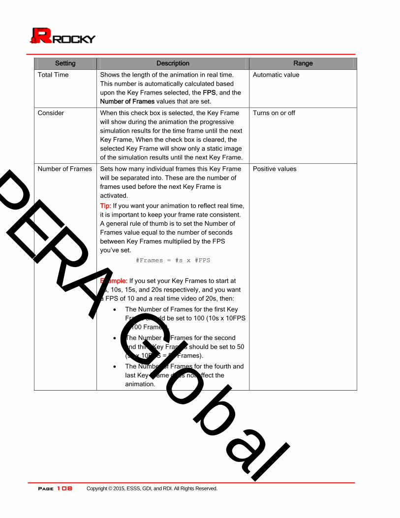
Page 108 Copyright © 2015, ESSS, GDI, and RDI. All Rights Reserved.
Setting Description Range
Total Time Shows the length of the animation in real time.
This number is automatically calculated based
upon the Key Frames selected, the FPS, and the
Number of Frames values that are set.
Automatic value
Consider When this check box is selected, the Key Frame
will show during the animation the progressive
simulation results for the time frame until the next
Key Frame, When the check box is cleared, the
selected Key Frame will show only a static image
of the simulation results until the next Key Frame.
Turns on or off
Number of Frames Sets how many individual frames this Key Frame
will be separated into. These are the number of
frames used before the next Key Frame is
activated.
Tip: If you want your animation to reflect real time,
it is important to keep your frame rate consistent.
A general rule of thumb is to set the Number of
Frames value equal to the number of seconds
between Key Frames multiplied by the FPS
you’ve set.
#Frames = #s x #FPS
Example: If you set your Key Frames to start at
0s, 10s, 15s, and 20s respectively, and you want
a FPS of 10 and a real time video of 20s, then:
The Number of Frames for the first Key
Frame should be set to 100 (10s x 10FPS
= 100 Frames).
The Number of Frames for the second
and third Key Frames should be set to 50
(5s x 10FPS = 50 Frames).
The Number of Frames for the fourth and
last Key Frame does not affect the
animation.
Positive values
安世
亚太
PERA Global

Copyright © 2015, ESSS, GDI, and RDI. All Rights Reserved. Page 109
Table 26: Video Compression Options
Setting Description Range
Compressor Type The method by which the movie will compress
when saved. In general:
Microsoft Video 1 will be a smaller file
size but will be less clear than full frames.
Full Frames (Uncompressed) will provide
the most clarity, but will be the biggest file
size.
Varies by video card. Consult the
manual of your particular video
card or software for more
information on the options
available to you.
Compression
Quality
Determines the compression ratio of the movie
when it is saved. In general, the higher the quality,
the clearer the image but the bigger the size of the
movie file.
0<100
Temporal Quality
Ratio
Helps determine the quality of your video
compression. Refer to your computer’s operating
system manual for more information.
0.01<1.00
To set up an animation
1. Open the simulation containing the results you want to animate.
2. Ensure the Animation panel is visible. (From the Tools menu, click Animation.)
3. Create a Key Frames list by doing the following:
a. Find or create a 3D View with the visualization settings you want to animate, including the rotation
and level of zoom.
b. Using the Timestep dropdown and/or arrows in the toolbar, choose the particular Timestep with
which you want your animation to start. (For example, if you want your animation to start at the
beginning, choose the [0] 0 s Timestep.)
c. From the bottom of the Animation panel, click the Add Key
Frame button.
An image of the Timestep and view you created shows in
the Key Frames list.
d. Set up your next Key Frame by doing one of the following:
To show the same view for a period of time, move only
your Timestep forward as desired but don’t change the
view.
To transition to another view over a period of time,
move your Timestep forward and change your view as
desired.
e. From the bottom of the Animation panel, click the Add Key
Frame button.
An image of the Timestep and view you created shows in
the Key Frames list.
f. Repeat steps 3d-e as many times as necessary to
Transition Tips:
To transition quickly between
views, leave no Timestep gap
between Key Frames.
To transition slowly between
views, leave a Timestep gap
between Key Frames equal to
the desired transition length.
To create a 360 wraparound
view, include two Key Frames
with the same exact view and
a Timestep gap equal to the
desired amount of time you
want the view to pivot around
the center point.
安世
亚太
PERA Global

Page 110 Copyright © 2015, ESSS, GDI, and RDI. All Rights Reserved.
complete your animation set up.
Tip: Use the buttons at the bottom and side of the Animation panel to help you delete, copy, move,
and update Key Frames that you’ve already created.
4. From the top of the Animation panel, determine what kind of transitions you want between your Key
Frames by choosing an option from the Camera Interpolation list.
5. Determine the speed, length, and quality of your animation by setting the values you want in the FPS
field for the animation, and Number of Frames field for each Key Frame. Use the values displayed for
Total Frames and Total Time to guide you in your selections.
6. At the bottom of the Animation panel, click the Play button to view a preview of your animation in the
Rocky Workspace, and then edit your Key Frames and animation options as desired.
To save an already set-up animation as an AVI
1. From the bottom of the Animation panel, click the Export Animation button, and then click AVI.
2. From the Export Animation to AVI dialog, choose the location to which you want to save the AVI file.
3. In the File name box, enter a name for the file, and then click Save.
4. From the Video Compression dialog, choose the Compressor type and Compressor Quality you want,
and then click Configure.
5. Verify that the Temporal Quality Ratio settings are set the way you want, and then click OK.
6. Click OK again to save the animation.
The Animation Export screen appears to show you the status of your save and a preview of the progress.
When the save is complete, the Animation Export screen disappears.
To save a static image of each individual frame in an animation
Tip: Before you start, review the Total Frames value displayed in the Animation panel to ensure you have set
up your animation the way you want. The number of images exported will equal this value.
1. From the bottom of the Animation panel, click the Export Animation button, and then click Images.
2. Form the Export Animation to Images dialog, choose the location to which you want to save the series of
images.
3. In the File name box, enter a name for the images and then from the Save as type list, choose what
image format you want.
4. Click Save.
The Animation Export screen appears to show you the status of your save and a preview of the progress.
When the save is complete, the Animation Export screen disappears.
Each image file name will be appended with the corresponding frame number.
安世
亚太
PERA Global

Copyright © 2015, ESSS, GDI, and RDI. All Rights Reserved. Page 111
6. Getting Help and Support
To get more help understanding the features and capabilities of Rocky, please consult the following
resources:
Rocky User Manual (this document). Use the Table of Contents at the beginning of the document or the
Search or Find function within your PDF viewer to quickly find the information you need.
To access the Rocky User Manual, from within the Rocky program, click User Manual from the Help
menu.
ESSS Customer Portal. View Rocky how-to and overview videos, installation instructions, and examples
of Rocky simulations. From the portal you can also submit a customer support request and check-up on
existing requests.
To access the ESSS customer portal, from the www.rocky-dem.com website, go to the Customer Portal
page, click the Customer Portal link, and then sign in as instructed. If you do not already have sign-in
information for the customer portal, please contact [email protected] for assistance.
Rocky Training. Sign-up for the next Rocky training session to get a better understanding of how Rocky
can help you improve your designs, and get hands-on experience using the product.
To learn more about Rocky training courses, please contact [email protected].
安世
亚太
PERA Global

Page 112 Copyright © 2015, ESSS, GDI, and RDI. All Rights Reserved.
7. Appendices
This section contains supplemental information that might assist you with using some of Rocky’s more advanced features.
What would you like to review?
Appendix A: Particle Shape Examples
Appendix B: ASCII Printable Characters
Appendix C: Calculation Reference
Appendix D: Use Variables to Test Varying Belt Speeds
安世
亚太
PERA Global

Copyright © 2015, ESSS, GDI, and RDI. All Rights Reserved. Page 113
Appendix A: Particle Shape Examples
Start with this
Particle Type To create this shape
Vertical
Aspect
Ratio
Horizontal
Aspect
Ratio
Smoothness Side
Angle
Number
of
Corners
Superquadric
Degree
Rounded
Polyhedron
Barley
2.7 1 0.163 N/A 48 2
Pea
1.08 1.08 0.964 N/A 25 2.6
Rice
2.55 0.9 0.964 N/A 16 2
Rock
1.5 0.75 0.25 N/A 15 2
Potato
0.7 1.7 1 N/A 27 2
Orange
1.1 1.1 1 N/A 104 2
Raisin
1.72 0.7 1 N/A 22 2.8
安世
亚太
PERA Global

Page 114 Copyright © 2015, ESSS, GDI, and RDI. All Rights Reserved.
Start with this
Particle Type To create this shape
Vertical
Aspect
Ratio
Horizontal
Aspect
Ratio
Smoothness Side
Angle
Number
of
Corners
Superquadric
Degree
Rounded
Polyhedron
Chocolate
1.26 1.26 1 N/A 40 10.5
Wood Chip
1.44 2.7 0.1 N/A 11 12
Coal
1.14 0.7 1 N/A 11 6.2
Rounded
Polygon
Poker Chip
1.05 0.1 N/A N/A 32 N/A
Corn
1.245 0.532 N/A N/A 5 N/A
Pill
1.215 0.532 N/A N/A 40 N/A
Navy Bean
1.8 0.9 N/A N/A 3 N/A
Sheet Metal
2.37 0.1 N/A N/A 4 N/A
安世
亚太
PERA Global

Copyright © 2015, ESSS, GDI, and RDI. All Rights Reserved. Page 115
Start with this
Particle Type To create this shape
Vertical
Aspect
Ratio
Horizontal
Aspect
Ratio
Smoothness Side
Angle
Number
of
Corners
Superquadric
Degree
Rounded
Cylinder
Rod
9.41 N/A N/A N/A N/A N/A
Capsule
2.57 N/A N/A N/A N/A N/A
Faceted
Sharp Rock
1.16 1.08 N/A N/A 10 2
Wafer
1.04 0.5 N/A N/A 57 2
Brick
0.5 1.76 N/A N/A 44 12
Firewood
0.7 2.5 N/A N/A 14 12
Briquette
Newspaper
0.6 2.005 N/A 5 60 N/A
Package
0.3 1.45 N/A 34.5 32 N/A
安世
亚太
PERA Global

Page 116 Copyright © 2015, ESSS, GDI, and RDI. All Rights Reserved.
Appendix B: ASCII Printable Characters
The below chart for the ASCII printable characters (codes 32-127) is useful for understanding how sort order
is determined in Rocky. (See also Name Components to Affect Sort Order).
Symbol Description
Space
! Exclamation mark
" Double quotes (or speech marks)
# Number
$ Dollar
% Percentage
& Ampersand
' Single quote
( Open parenthesis (or open bracket)
) Close parenthesis (or close bracket)
* Asterisk
+ Plus
, Comma
- Hyphen
. Period, dot, or full stop
/ Slash or divide
0 Zero
1 One
2 Two
3 Three
4 Four
5 Five
6 Six
7 Seven
8 Eight
9 Nine
: Colon
; Semicolon
< Less than (or open angled bracket)
= Equals
> Greater than (or close angled bracket)
? Question mark
@ At symbol
A Uppercase A
B Uppercase B
C Uppercase C
D Uppercase D
E Uppercase E
F Uppercase F
G Uppercase G
H Uppercase H
安世
亚太
PERA Global

Copyright © 2015, ESSS, GDI, and RDI. All Rights Reserved. Page 117
I Uppercase I
J Uppercase J
K Uppercase K
L Uppercase L
M Uppercase M
N Uppercase N
O Uppercase O
P Uppercase P
Q Uppercase Q
R Uppercase R
S Uppercase S
T Uppercase T
U Uppercase U
V Uppercase V
W Uppercase W
X Uppercase X
Y Uppercase Y
Z Uppercase Z
[ Opening bracket
\ Backslash
] Closing bracket
^ Caret - circumflex
_ Underscore
` Grave accent
a Lowercase a
b Lowercase b
c Lowercase c
d Lowercase d
e Lowercase e
f Lowercase f
g Lowercase g
h Lowercase h
i Lowercase i
j Lowercase j
k Lowercase k
l Lowercase l
m Lowercase m
n Lowercase n
o Lowercase o
p Lowercase p
q Lowercase q
r Lowercase r
s Lowercase s
t Lowercase t
u Lowercase u
v Lowercase v
w Lowercase w
安世
亚太
PERA Global

Page 118 Copyright © 2015, ESSS, GDI, and RDI. All Rights Reserved.
x Lowercase x
y Lowercase y
z Lowercase z
{ Opening brace
| Vertical bar
} Closing brace
~ Equivalency sign - tilde
Delete
安世
亚太
PERA Global

Copyright © 2015, ESSS, GDI, and RDI. All Rights Reserved. Page 119
Appendix C: Calculation Reference
Rocky uses expressions to create a new curve or grid function. These expressions are based upon the latest
NumPy math routines. (For more information about NumPy math routines, see
http://docs.scipy.org/doc/numpy/reference/routines.math.html).
Some examples of operations using curves or grid functions are as follows:
A+B
log(A)
A+(B-100)
It is also possible to conduct calculations using timesteps, in which case the expression would access the
variables using brackets [ ].
For example:
A[t]-A[t-1] would give the delta between 2 timesteps.
A[t]-A[0] would give the delta from the current time to the first timestep.
Use the Table of Functions below to navigate to the section you are interested in.
Table of Functions
Trigonometric functions ......................................................................................................................... 121
sin ...................................................................................................................................................................... 121 cos ..................................................................................................................................................................... 122 tan ...................................................................................................................................................................... 123 arcsin ................................................................................................................................................................. 124 arccos ................................................................................................................................................................ 126 arctan ................................................................................................................................................................. 127 hypot .................................................................................................................................................................. 129
arctan2 ............................................................................................................................................................... 129 degrees .............................................................................................................................................................. 131 radians ............................................................................................................................................................... 132 unwrap ............................................................................................................................................................... 133 deg2rad .............................................................................................................................................................. 133 rad2deg .............................................................................................................................................................. 134
Hyperbolic functions .............................................................................................................................. 135
sinh .................................................................................................................................................................... 135 cosh ................................................................................................................................................................... 136 tanh .................................................................................................................................................................... 137
arcsinh ............................................................................................................................................................... 138 arccosh .............................................................................................................................................................. 139 arctanh ............................................................................................................................................................... 140
Rounding ............................................................................................................................................... 141
around ................................................................................................................................................................ 141
安世
亚太
PERA Global

Page 120 Copyright © 2015, ESSS, GDI, and RDI. All Rights Reserved.
round .................................................................................................................................................................. 143 rint ...................................................................................................................................................................... 143 fix ....................................................................................................................................................................... 143 floor .................................................................................................................................................................... 144 ceil ..................................................................................................................................................................... 145 trunc ................................................................................................................................................................... 146
Sums, products, differences .................................................................................................................. 146
prod .................................................................................................................................................................... 146 sum .................................................................................................................................................................... 148 nansum .............................................................................................................................................................. 149 cumprod ............................................................................................................................................................. 151 cumsum ............................................................................................................................................................. 152 diff ...................................................................................................................................................................... 153 ediff1d ................................................................................................................................................................ 154 gradient .............................................................................................................................................................. 155 cross .................................................................................................................................................................. 156 trapz ................................................................................................................................................................... 158
Exponents and logarithms ..................................................................................................................... 160
exp ..................................................................................................................................................................... 160 expm1 ................................................................................................................................................................ 161 log ...................................................................................................................................................................... 162 log10 .................................................................................................................................................................. 163 log2 .................................................................................................................................................................... 164 log1p .................................................................................................................................................................. 165 logaddexp .......................................................................................................................................................... 167 logaddexp2 ........................................................................................................................................................ 167
Other special functions .......................................................................................................................... 168
i0 ........................................................................................................................................................................ 168 sinc .................................................................................................................................................................... 170
Floating point routines ........................................................................................................................... 171
signbit ................................................................................................................................................................ 171 copysign ............................................................................................................................................................. 172 frexp ................................................................................................................................................................... 173 ldexp .................................................................................................................................................................. 173
Arithmetic operations ............................................................................................................................. 173
add ..................................................................................................................................................................... 173 reciprocal ........................................................................................................................................................... 174 negative ............................................................................................................................................................. 174 multiply............................................................................................................................................................... 175 divide ................................................................................................................................................................. 176 power ................................................................................................................................................................. 177
subtract .............................................................................................................................................................. 178 true_divide ......................................................................................................................................................... 179 floor_divide ........................................................................................................................................................ 180 fmod ................................................................................................................................................................... 181 mod .................................................................................................................................................................... 182
安世
亚太
PERA Global

Copyright © 2015, ESSS, GDI, and RDI. All Rights Reserved. Page 121
modf ................................................................................................................................................................... 183 remainder ........................................................................................................................................................... 183
Handling complex numbers ................................................................................................................... 184
angle .................................................................................................................................................................. 184 real ..................................................................................................................................................................... 185 imag ................................................................................................................................................................... 185 conj .................................................................................................................................................................... 186
Miscellaneous ........................................................................................................................................ 187
convolve ............................................................................................................................................................. 187 clip ...................................................................................................................................................................... 189 sqrt ..................................................................................................................................................................... 190 square ................................................................................................................................................................ 191 absolute ............................................................................................................................................................. 191 abs ..................................................................................................................................................................... 192 fabs .................................................................................................................................................................... 193 sign .................................................................................................................................................................... 194 maximum............................................................................................................................................................ 194 max .................................................................................................................................................................... 195 minimum ............................................................................................................................................................ 197 min ..................................................................................................................................................................... 198 nan_to_num ....................................................................................................................................................... 199 real_if_close ....................................................................................................................................................... 200 interp .................................................................................................................................................................. 201
Trigonometric functions
sin
sin(x[, out])
Trigonometric sine, element-wise.
Parameters
----------
x : array_like
Angle, in radians (:math:`2 \pi` rad equals 360 degrees).
Returns
-------
y : array_like
The sine of each element of x.
See Also
--------
arcsin, sinh, cos
安世
亚太
PERA Global

Page 122 Copyright © 2015, ESSS, GDI, and RDI. All Rights Reserved.
Notes
-----
The sine is one of the fundamental functions of trigonometry
(the mathematical study of triangles). Consider a circle of radius
1 centered on the origin. A ray comes in from the :math:`+x` axis,
makes an angle at the origin (measured counter-clockwise from that
axis), and departs from the origin. The :math:`y` coordinate of
the outgoing ray's intersection with the unit circle is the sine
of that angle. It ranges from -1 for :math:`x=3\pi / 2` to
+1 for :math:`\pi / 2.` The function has zeroes where the angle is
a multiple of :math:`\pi`. Sines of angles between :math:`\pi` and
:math:`2\pi` are negative. The numerous properties of the sine and
related functions are included in any standard trigonometry text.
Examples
--------
Print sine of one angle:
>>> np.sin(np.pi/2.)
1.0
Print sines of an array of angles given in degrees:
>>> np.sin(np.array((0., 30., 45., 60., 90.)) * np.pi / 180. )
array([ 0. , 0.5 , 0.70710678, 0.8660254 , 1. ])
Plot the sine function:
>>> import matplotlib.pylab as plt
>>> x = np.linspace(-np.pi, np.pi, 201)
>>> plt.plot(x, np.sin(x))
>>> plt.xlabel('Angle [rad]')
>>> plt.ylabel('sin(x)')
>>> plt.axis('tight')
>>> plt.show()
cos
cos(x[, out])
Cosine elementwise.
Parameters
----------
x : array_like
Input array in radians.
out : ndarray, optional
安世
亚太
PERA Global

Copyright © 2015, ESSS, GDI, and RDI. All Rights Reserved. Page 123
Output array of same shape as `x`.
Returns
-------
y : ndarray
The corresponding cosine values.
Raises
------
ValueError: invalid return array shape
if `out` is provided and `out.shape` != `x.shape` (See Examples)
Notes
-----
If `out` is provided, the function writes the result into it,
and returns a reference to `out`. (See Examples)
References
----------
M. Abramowitz and I. A. Stegun, Handbook of Mathematical Functions.
New York, NY: Dover, 1972.
Examples
--------
>>> np.cos(np.array([0, np.pi/2, np.pi]))
array([ 1.00000000e+00, 6.12303177e-17, -1.00000000e+00])
>>>
>>> # Example of providing the optional output parameter
>>> out2 = np.cos([0.1], out1)
>>> out2 is out1
True
>>>
>>> # Example of ValueError due to provision of shape mis-matched `out`
>>> np.cos(np.zeros((3,3)),np.zeros((2,2)))
Traceback (most recent call last):
File "", line 1, in
ValueError: invalid return array shape
tan
tan(x[, out])
Compute tangent element-wise.
Equivalent to ``np.sin(x)/np.cos(x)`` element-wise.
Parameters
安世
亚太
PERA Global

Page 124 Copyright © 2015, ESSS, GDI, and RDI. All Rights Reserved.
----------
x : array_like
Input array.
out : ndarray, optional
Output array of same shape as `x`.
Returns
-------
y : ndarray
The corresponding tangent values.
Raises
------
ValueError: invalid return array shape
if `out` is provided and `out.shape` != `x.shape` (See Examples)
Notes
-----
If `out` is provided, the function writes the result into it,
and returns a reference to `out`. (See Examples)
References
----------
M. Abramowitz and I. A. Stegun, Handbook of Mathematical Functions.
New York, NY: Dover, 1972.
Examples
--------
>>> from math import pi
>>> np.tan(np.array([-pi,pi/2,pi]))
array([ 1.22460635e-16, 1.63317787e+16, -1.22460635e-16])
>>>
>>> # Example of providing the optional output parameter illustrating
>>> # that what is returned is a reference to said parameter
>>> out2 = np.cos([0.1], out1)
>>> out2 is out1
True
>>>
>>> # Example of ValueError due to provision of shape mis-matched `out`
>>> np.cos(np.zeros((3,3)),np.zeros((2,2)))
Traceback (most recent call last):
File "", line 1, in
ValueError: invalid return array shape
arcsin
安世
亚太
PERA Global

Copyright © 2015, ESSS, GDI, and RDI. All Rights Reserved. Page 125
arcsin(x[, out])
Inverse sine, element-wise.
Parameters
----------
x : array_like
`y`-coordinate on the unit circle.
out : ndarray, optional
Array of the same shape as `x`, in which to store the results.
See `doc.ufuncs` (Section "Output arguments") for more details.
Returns
-------
angle : ndarray
The inverse sine of each element in `x`, in radians and in the
closed interval ``[-pi/2, pi/2]``. If `x` is a scalar, a scalar
is returned, otherwise an array.
See Also
--------
sin, cos, arccos, tan, arctan, arctan2, emath.arcsin
Notes
-----
`arcsin` is a multivalued function: for each `x` there are infinitely
many numbers `z` such that :math:`sin(z) = x`. The convention is to
return the angle `z` whose real part lies in [-pi/2, pi/2].
For real-valued input data types, *arcsin* always returns real output.
For each value that cannot be expressed as a real number or infinity,
it yields ``nan`` and sets the `invalid` floating point error flag.
For complex-valued input, `arcsin` is a complex analytic function that
has, by convention, the branch cuts [-inf, -1] and [1, inf] and is
continuous from above on the former and from below on the latter.
The inverse sine is also known as `asin` or sin^{-1}.
References
----------
Abramowitz, M. and Stegun, I. A., *Handbook of Mathematical Functions*,
10th printing, New York: Dover, 1964, pp. 79ff.
http://www.math.sfu.ca/~cbm/aands/
Examples
安世
亚太
PERA Global

Page 126 Copyright © 2015, ESSS, GDI, and RDI. All Rights Reserved.
--------
>>> np.arcsin(1) # pi/2
1.5707963267948966
>>> np.arcsin(-1) # -pi/2
-1.5707963267948966
>>> np.arcsin(0)
0.0
arccos
arccos(x[, out])
Trigonometric inverse cosine, element-wise.
The inverse of `cos` so that, if ``y = cos(x)``, then ``x = arccos(y)``.
Parameters
----------
x : array_like
`x`-coordinate on the unit circle.
For real arguments, the domain is [-1, 1].
out : ndarray, optional
Array of the same shape as `a`, to store results in. See
`doc.ufuncs` (Section "Output arguments") for more details.
Returns
-------
angle : ndarray
The angle of the ray intersecting the unit circle at the given
`x`-coordinate in radians [0, pi]. If `x` is a scalar then a
scalar is returned, otherwise an array of the same shape as `x`
is returned.
See Also
--------
cos, arctan, arcsin, emath.arccos
Notes
-----
`arccos` is a multivalued function: for each `x` there are infinitely
many numbers `z` such that `cos(z) = x`. The convention is to return
the angle `z` whose real part lies in `[0, pi]`.
For real-valued input data types, `arccos` always returns real output.
For each value that cannot be expressed as a real number or infinity,
it yields ``nan`` and sets the `invalid` floating point error flag.
安世
亚太
PERA Global

Copyright © 2015, ESSS, GDI, and RDI. All Rights Reserved. Page 127
For complex-valued input, `arccos` is a complex analytic function that
has branch cuts `[-inf, -1]` and `[1, inf]` and is continuous from
above on the former and from below on the latter.
The inverse `cos` is also known as `acos` or cos^-1.
References
----------
M. Abramowitz and I.A. Stegun, "Handbook of Mathematical Functions",
10th printing, 1964, pp. 79. http://www.math.sfu.ca/~cbm/aands/
Examples
--------
We expect the arccos of 1 to be 0, and of -1 to be pi:
>>> np.arccos([1, -1])
array([ 0. , 3.14159265])
Plot arccos:
>>> import matplotlib.pyplot as plt
>>> x = np.linspace(-1, 1, num=100)
>>> plt.plot(x, np.arccos(x))
>>> plt.axis('tight')
>>> plt.show()
arctan
arctan(x[, out])
Trigonometric inverse tangent, element-wise.
The inverse of tan, so that if ``y = tan(x)`` then ``x = arctan(y)``.
Parameters
----------
x : array_like
Input values. `arctan` is applied to each element of `x`.
Returns
-------
out : ndarray
Out has the same shape as `x`. Its real part is in
``[-pi/2, pi/2]`` (``arctan(+/-inf)`` returns ``+/-pi/2``).
It is a scalar if `x` is a scalar.
安世
亚太
PERA Global

Page 128 Copyright © 2015, ESSS, GDI, and RDI. All Rights Reserved.
See Also
--------
arctan2 : The "four quadrant" arctan of the angle formed by (`x`, `y`)
and the positive `x`-axis.
angle : Argument of complex values.
Notes
-----
`arctan` is a multi-valued function: for each `x` there are infinitely
many numbers `z` such that tan(`z`) = `x`. The convention is to return
the angle `z` whose real part lies in [-pi/2, pi/2].
For real-valued input data types, `arctan` always returns real output.
For each value that cannot be expressed as a real number or infinity,
it yields ``nan`` and sets the `invalid` floating point error flag.
For complex-valued input, `arctan` is a complex analytic function that
has [`1j, infj`] and [`-1j, -infj`] as branch cuts, and is continuous
from the left on the former and from the right on the latter.
The inverse tangent is also known as `atan` or tan^{-1}.
References
----------
Abramowitz, M. and Stegun, I. A., *Handbook of Mathematical Functions*,
10th printing, New York: Dover, 1964, pp. 79.
http://www.math.sfu.ca/~cbm/aands/
Examples
--------
We expect the arctan of 0 to be 0, and of 1 to be pi/4:
>>> np.arctan([0, 1])
array([ 0. , 0.78539816])
>>> np.pi/4
0.78539816339744828
Plot arctan:
>>> import matplotlib.pyplot as plt
>>> x = np.linspace(-10, 10)
>>> plt.plot(x, np.arctan(x))
>>> plt.axis('tight')
>>> plt.show()
安世
亚太
PERA Global

Copyright © 2015, ESSS, GDI, and RDI. All Rights Reserved. Page 129
hypot
hypot(x1, x2[, out])
Given the "legs" of a right triangle, return its hypotenuse.
Equivalent to ``sqrt(x1**2 + x2**2)``, element-wise. If `x1` or
`x2` is scalar_like (i.e., unambiguously cast-able to a scalar type),
it is broadcast for use with each element of the other argument.
(See Examples)
Parameters
----------
x1, x2 : array_like
Leg of the triangle(s).
out : ndarray, optional
Array into which the output is placed. Its type is preserved and it
must be of the right shape to hold the output. See doc.ufuncs.
Returns
-------
z : ndarray
The hypotenuse of the triangle(s).
Examples
--------
>>> np.hypot(3*np.ones((3, 3)), 4*np.ones((3, 3)))
array([[ 5., 5., 5.],
[ 5., 5., 5.],
[ 5., 5., 5.]])
Example showing broadcast of scalar_like argument:
>>> np.hypot(3*np.ones((3, 3)), [4])
array([[ 5., 5., 5.],
[ 5., 5., 5.],
[ 5., 5., 5.]])
arctan2
arctan2(x1, x2[, out])
Element-wise arc tangent of ``x1/x2`` choosing the quadrant correctly.
The quadrant (i.e., branch) is chosen so that ``arctan2(x1, x2)`` is
the signed angle in radians between the ray ending at the origin and
passing through the point (1,0), and the ray ending at the origin and
安世
亚太
PERA Global

Page 130 Copyright © 2015, ESSS, GDI, and RDI. All Rights Reserved.
passing through the point (`x2`, `x1`). (Note the role reversal: the
"`y`-coordinate" is the first function parameter, the "`x`-coordinate"
is the second.) By IEEE convention, this function is defined for
`x2` = +/-0 and for either or both of `x1` and `x2` = +/-inf (see
Notes for specific values).
This function is not defined for complex-valued arguments; for the
so-called argument of complex values, use `angle`.
Parameters
----------
x1 : array_like, real-valued
`y`-coordinates.
x2 : array_like, real-valued
`x`-coordinates. `x2` must be broadcastable to match the shape of
`x1` or vice versa.
Returns
-------
angle : ndarray
Array of angles in radians, in the range ``[-pi, pi]``.
See Also
--------
arctan, tan, angle
Notes
-----
*arctan2* is identical to the `atan2` function of the underlying
C library. The following special values are defined in the C
standard: [1]_
====== ====== ================
`x1` `x2` `arctan2(x1,x2)`
====== ====== ================
+/- 0 +0 +/- 0
+/- 0 -0 +/- pi
> 0 +/-inf +0 / +pi
< 0 +/-inf -0 / -pi
+/-inf +inf +/- (pi/4)
+/-inf -inf +/- (3*pi/4)
====== ====== ================
Note that +0 and -0 are distinct floating point numbers, as are +inf
and -inf.
References
安世
亚太
PERA Global

Copyright © 2015, ESSS, GDI, and RDI. All Rights Reserved. Page 131
----------
.. [1] ISO/IEC standard 9899:1999, "Programming language C."
Examples
--------
Consider four points in different quadrants:
>>> x = np.array([-1, +1, +1, -1])
>>> y = np.array([-1, -1, +1, +1])
>>> np.arctan2(y, x) * 180 / np.pi
array([-135., -45., 45., 135.])
Note the order of the parameters. `arctan2` is defined also when `x2` = 0
and at several other special points, obtaining values in
the range ``[-pi, pi]``:
>>> np.arctan2([1., -1.], [0., 0.])
array([ 1.57079633, -1.57079633])
>>> np.arctan2([0., 0., np.inf], [+0., -0., np.inf])
array([ 0. , 3.14159265, 0.78539816])
degrees
degrees(x[, out])
Convert angles from radians to degrees.
Parameters
----------
x : array_like
Input array in radians.
out : ndarray, optional
Output array of same shape as x.
Returns
-------
y : ndarray of floats
The corresponding degree values; if `out` was supplied this is a
reference to it.
See Also
--------
rad2deg : equivalent function
Examples
--------
Convert a radian array to degrees
安世
亚太
PERA Global

Page 132 Copyright © 2015, ESSS, GDI, and RDI. All Rights Reserved.
>>> rad = np.arange(12.)*np.pi/6
>>> np.degrees(rad)
array([ 0., 30., 60., 90., 120., 150., 180., 210., 240.,
270., 300., 330.])
>>> out = np.zeros((rad.shape))
>>> r = degrees(rad, out)
>>> np.all(r == out)
True
radians
radians(x[, out])
Convert angles from degrees to radians.
Parameters
----------
x : array_like
Input array in degrees.
out : ndarray, optional
Output array of same shape as `x`.
Returns
-------
y : ndarray
The corresponding radian values.
See Also
--------
deg2rad : equivalent function
Examples
--------
Convert a degree array to radians
>>> deg = np.arange(12.) * 30.
>>> np.radians(deg)
array([ 0. , 0.52359878, 1.04719755, 1.57079633, 2.0943951 ,
2.61799388, 3.14159265, 3.66519143, 4.1887902 , 4.71238898,
5.23598776, 5.75958653])
>>> out = np.zeros((deg.shape))
>>> ret = np.radians(deg, out)
>>> ret is out
True
安世
亚太
PERA Global

Copyright © 2015, ESSS, GDI, and RDI. All Rights Reserved. Page 133
unwrap
Unwrap by changing deltas between values to 2*pi complement.
Unwrap radian phase `p` by changing absolute jumps greater than
`discont` to their 2*pi complement along the given axis.
Parameters
----------
p : array_like
Input array.
discont : float, optional
Maximum discontinuity between values, default is ``pi``.
axis : int, optional
Axis along which unwrap will operate, default is the last axis.
Returns
-------
out : ndarray
Output array.
See Also
--------
rad2deg, deg2rad
Notes
-----
If the discontinuity in `p` is smaller than ``pi``, but larger than
`discont`, no unwrapping is done because taking the 2*pi complement
would only make the discontinuity larger.
Examples
--------
>>> phase = np.linspace(0, np.pi, num=5)
>>> phase[3:] += np.pi
>>> phase
array([ 0. , 0.78539816, 1.57079633, 5.49778714, 6.28318531])
>>> np.unwrap(phase)
array([ 0. , 0.78539816, 1.57079633, -0.78539816, 0. ])
deg2rad
deg2rad(x[, out])
Convert angles from degrees to radians.
安世
亚太
PERA Global

Page 134 Copyright © 2015, ESSS, GDI, and RDI. All Rights Reserved.
Parameters
----------
x : array_like
Angles in degrees.
Returns
-------
y : ndarray
The corresponding angle in radians.
See Also
--------
rad2deg : Convert angles from radians to degrees.
unwrap : Remove large jumps in angle by wrapping.
Notes
-----
.. versionadded:: 1.3.0
``deg2rad(x)`` is ``x * pi / 180``.
Examples
--------
>>> np.deg2rad(180)
3.1415926535897931
rad2deg
rad2deg(x[, out])
Convert angles from radians to degrees.
Parameters
----------
x : array_like
Angle in radians.
out : ndarray, optional
Array into which the output is placed. Its type is preserved and it
must be of the right shape to hold the output. See doc.ufuncs.
Returns
-------
y : ndarray
The corresponding angle in degrees.
See Also
--------
安世
亚太
PERA Global

Copyright © 2015, ESSS, GDI, and RDI. All Rights Reserved. Page 135
deg2rad : Convert angles from degrees to radians.
unwrap : Remove large jumps in angle by wrapping.
Notes
-----
.. versionadded:: 1.3.0
rad2deg(x) is ``180 * x / pi``.
Examples
--------
>>> np.rad2deg(np.pi/2)
90.0
Hyperbolic functions
sinh
sinh(x[, out])
Hyperbolic sine, element-wise.
Equivalent to ``1/2 * (np.exp(x) - np.exp(-x))`` or
``-1j * np.sin(1j*x)``.
Parameters
----------
x : array_like
Input array.
out : ndarray, optional
Output array of same shape as `x`.
Returns
-------
y : ndarray
The corresponding hyperbolic sine values.
Raises
------
ValueError: invalid return array shape
if `out` is provided and `out.shape` != `x.shape` (See Examples)
Notes
-----
安世
亚太
PERA Global

Page 136 Copyright © 2015, ESSS, GDI, and RDI. All Rights Reserved.
If `out` is provided, the function writes the result into it,
and returns a reference to `out`. (See Examples)
References
----------
M. Abramowitz and I. A. Stegun, Handbook of Mathematical Functions.
New York, NY: Dover, 1972, pg. 83.
Examples
--------
>>> np.sinh(0)
0.0
>>> np.sinh(np.pi*1j/2)
1j
>>> np.sinh(np.pi*1j) # (exact value is 0)
1.2246063538223773e-016j
>>> # Discrepancy due to vagaries of floating point arithmetic.
>>> # Example of providing the optional output parameter
>>> out2 = np.sinh([0.1], out1)
>>> out2 is out1
True
>>> # Example of ValueError due to provision of shape mis-matched `out`
>>> np.sinh(np.zeros((3,3)),np.zeros((2,2)))
Traceback (most recent call last):
File "", line 1, in
ValueError: invalid return array shape
cosh
cosh(x[, out])
Hyperbolic cosine, element-wise.
Equivalent to ``1/2 * (np.exp(x) + np.exp(-x))`` and ``np.cos(1j*x)``.
Parameters
----------
x : array_like
Input array.
Returns
-------
out : ndarray
Output array of same shape as `x`.
安世
亚太
PERA Global
Copyright © 2015, ESSS, GDI, and RDI. All Rights Reserved. Page 137
Examples
--------
>>> np.cosh(0)
1.0
The hyperbolic cosine describes the shape of a hanging cable:
>>> import matplotlib.pyplot as plt
>>> x = np.linspace(-4, 4, 1000)
>>> plt.plot(x, np.cosh(x))
>>> plt.show()
tanh
tanh(x[, out])
Compute hyperbolic tangent element-wise.
Equivalent to ``np.sinh(x)/np.cosh(x)`` or
``-1j * np.tan(1j*x)``.
Parameters
----------
x : array_like
Input array.
out : ndarray, optional
Output array of same shape as `x`.
Returns
-------
y : ndarray
The corresponding hyperbolic tangent values.
Raises
------
ValueError: invalid return array shape
if `out` is provided and `out.shape` != `x.shape` (See Examples)
Notes
-----
If `out` is provided, the function writes the result into it,
and returns a reference to `out`. (See Examples)
References
----------
.. [1] M. Abramowitz and I. A. Stegun, Handbook of Mathematical Functions.
New York, NY: Dover, 1972, pg. 83.
安世
亚太
PERA Global

Page 138 Copyright © 2015, ESSS, GDI, and RDI. All Rights Reserved.
http://www.math.sfu.ca/~cbm/aands/
.. [2] Wikipedia, "Hyperbolic function",
http://en.wikipedia.org/wiki/Hyperbolic_function
Examples
--------
>>> np.tanh((0, np.pi*1j, np.pi*1j/2))
array([ 0. +0.00000000e+00j, 0. -1.22460635e-16j, 0. +1.63317787e+16j])
>>> # Example of providing the optional output parameter illustrating
>>> # that what is returned is a reference to said parameter
>>> out2 = np.tanh([0.1], out1)
>>> out2 is out1
True
>>> # Example of ValueError due to provision of shape mis-matched `out`
>>> np.tanh(np.zeros((3,3)),np.zeros((2,2)))
Traceback (most recent call last):
File "", line 1, in
ValueError: invalid return array shape
arcsinh
arcsinh(x[, out])
Inverse hyperbolic sine elementwise.
Parameters
----------
x : array_like
Input array.
out : ndarray, optional
Array into which the output is placed. Its type is preserved and it
must be of the right shape to hold the output. See `doc.ufuncs`.
Returns
-------
out : ndarray
Array of of the same shape as `x`.
Notes
-----
`arcsinh` is a multivalued function: for each `x` there are infinitely
many numbers `z` such that `sinh(z) = x`. The convention is to return the
`z` whose imaginary part lies in `[-pi/2, pi/2]`.
安世
亚太
PERA Global

Copyright © 2015, ESSS, GDI, and RDI. All Rights Reserved. Page 139
For real-valued input data types, `arcsinh` always returns real output.
For each value that cannot be expressed as a real number or infinity, it
returns ``nan`` and sets the `invalid` floating point error flag.
For complex-valued input, `arccos` is a complex analytical function that
has branch cuts `[1j, infj]` and `[-1j, -infj]` and is continuous from
the right on the former and from the left on the latter.
The inverse hyperbolic sine is also known as `asinh` or ``sinh^-1``.
References
----------
.. [1] M. Abramowitz and I.A. Stegun, "Handbook of Mathematical Functions",
10th printing, 1964, pp. 86. http://www.math.sfu.ca/~cbm/aands/
.. [2] Wikipedia, "Inverse hyperbolic function",
http://en.wikipedia.org/wiki/Arcsinh
Examples
--------
>>> np.arcsinh(np.array([np.e, 10.0]))
array([ 1.72538256, 2.99822295])
arccosh
arccosh(x[, out])
Inverse hyperbolic cosine, elementwise.
Parameters
----------
x : array_like
Input array.
out : ndarray, optional
Array of the same shape as `x`, to store results in.
See `doc.ufuncs` (Section "Output arguments") for details.
Returns
-------
y : ndarray
Array of the same shape as `x`.
See Also
--------
cosh, arcsinh, sinh, arctanh, tanh
安世
亚太
PERA Global

Page 140 Copyright © 2015, ESSS, GDI, and RDI. All Rights Reserved.
Notes
-----
`arccosh` is a multivalued function: for each `x` there are infinitely
many numbers `z` such that `cosh(z) = x`. The convention is to return the
`z` whose imaginary part lies in `[-pi, pi]` and the real part in
``[0, inf]``.
For real-valued input data types, `arccosh` always returns real output.
For each value that cannot be expressed as a real number or infinity, it
yields ``nan`` and sets the `invalid` floating point error flag.
For complex-valued input, `arccosh` is a complex analytical function that
has a branch cut `[-inf, 1]` and is continuous from above on it.
References
----------
.. [1] M. Abramowitz and I.A. Stegun, "Handbook of Mathematical Functions",
10th printing, 1964, pp. 86. http://www.math.sfu.ca/~cbm/aands/
.. [2] Wikipedia, "Inverse hyperbolic function",
http://en.wikipedia.org/wiki/Arccosh
Examples
--------
>>> np.arccosh([np.e, 10.0])
array([ 1.65745445, 2.99322285])
>>> np.arccosh(1)
0.0
arctanh
arctanh(x[, out])
Inverse hyperbolic tangent elementwise.
Parameters
----------
x : array_like
Input array.
Returns
-------
out : ndarray
Array of the same shape as `x`.
See Also
--------
emath.arctanh
安世
亚太
PERA Global

Copyright © 2015, ESSS, GDI, and RDI. All Rights Reserved. Page 141
Notes
-----
`arctanh` is a multivalued function: for each `x` there are infinitely
many numbers `z` such that `tanh(z) = x`. The convention is to return the
`z` whose imaginary part lies in `[-pi/2, pi/2]`.
For real-valued input data types, `arctanh` always returns real output.
For each value that cannot be expressed as a real number or infinity, it
yields ``nan`` and sets the `invalid` floating point error flag.
For complex-valued input, `arctanh` is a complex analytical function that
has branch cuts `[-1, -inf]` and `[1, inf]` and is continuous from
above on the former and from below on the latter.
The inverse hyperbolic tangent is also known as `atanh` or ``tanh^-1``.
References
----------
.. [1] M. Abramowitz and I.A. Stegun, "Handbook of Mathematical Functions",
10th printing, 1964, pp. 86. http://www.math.sfu.ca/~cbm/aands/
.. [2] Wikipedia, "Inverse hyperbolic function",
http://en.wikipedia.org/wiki/Arctanh
Examples
--------
>>> np.arctanh([0, -0.5])
array([ 0. , -0.54930614])
Rounding
around
Evenly round to the given number of decimals.
Parameters
----------
a : array_like
Input data.
decimals : int, optional
Number of decimal places to round to (default: 0). If
decimals is negative, it specifies the number of positions to
the left of the decimal point.
out : ndarray, optional
安世
亚太
PERA Global

Page 142 Copyright © 2015, ESSS, GDI, and RDI. All Rights Reserved.
Alternative output array in which to place the result. It must have
the same shape as the expected output, but the type of the output
values will be cast if necessary. See `doc.ufuncs` (Section
"Output arguments") for details.
Returns
-------
rounded_array : ndarray
An array of the same type as `a`, containing the rounded values.
Unless `out` was specified, a new array is created. A reference to
the result is returned.
The real and imaginary parts of complex numbers are rounded
separately. The result of rounding a float is a float.
See Also
--------
ndarray.round : equivalent method
ceil, fix, floor, rint, trunc
Notes
-----
For values exactly halfway between rounded decimal values, Numpy
rounds to the nearest even value. Thus 1.5 and 2.5 round to 2.0,
-0.5 and 0.5 round to 0.0, etc. Results may also be surprising due
to the inexact representation of decimal fractions in the IEEE
floating point standard [1]_ and errors introduced when scaling
by powers of ten.
References
----------
.. [1] "Lecture Notes on the Status of IEEE 754", William Kahan,
http://www.cs.berkeley.edu/~wkahan/ieee754status/IEEE754.PDF
.. [2] "How Futile are Mindless Assessments of
Roundoff in Floating-Point Computation?", William Kahan,
http://www.cs.berkeley.edu/~wkahan/Mindless.pdf
Examples
--------
>>> np.around([0.37, 1.64])
array([ 0., 2.])
>>> np.around([0.37, 1.64], decimals=1)
array([ 0.4, 1.6])
>>> np.around([.5, 1.5, 2.5, 3.5, 4.5]) # rounds to nearest even value
array([ 0., 2., 2., 4., 4.])
安世
亚太
PERA Global

Copyright © 2015, ESSS, GDI, and RDI. All Rights Reserved. Page 143
>>> np.around([1,2,3,11], decimals=1) # ndarray of ints is returned
array([ 1, 2, 3, 11])
>>> np.around([1,2,3,11], decimals=-1)
array([ 0, 0, 0, 10])
round
Round an array to the given number of decimals.
Refer to `around` for full documentation.
See Also
--------
around : equivalent function
rint
rint(x[, out])
Round elements of the array to the nearest integer.
Parameters
----------
x : array_like
Input array.
Returns
-------
out : {ndarray, scalar}
Output array is same shape and type as `x`.
See Also
--------
ceil, floor, trunc
Examples
--------
>>> a = np.array([-1.7, -1.5, -0.2, 0.2, 1.5, 1.7, 2.0])
>>> np.rint(a)
array([-2., -2., -0., 0., 2., 2., 2.])
fix
Round to nearest integer towards zero.
安世
亚太
PERA Global

Page 144 Copyright © 2015, ESSS, GDI, and RDI. All Rights Reserved.
Round an array of floats element-wise to nearest integer towards zero.
The rounded values are returned as floats.
Parameters
----------
x : array_like
An array of floats to be rounded
y : ndarray, optional
Output array
Returns
-------
out : ndarray of floats
The array of rounded numbers
See Also
--------
trunc, floor, ceil
around : Round to given number of decimals
Examples
--------
>>> np.fix(3.14)
3.0
>>> np.fix(3)
3.0
>>> np.fix([2.1, 2.9, -2.1, -2.9])
array([ 2., 2., -2., -2.])
floor
floor(x[, out])
Return the floor of the input, element-wise.
The floor of the scalar `x` is the largest integer `i`, such that
`i <= x`. It is often denoted as :math:`\lfloor x \rfloor`.
Parameters
----------
x : array_like
Input data.
Returns
-------
y : {ndarray, scalar}
The floor of each element in `x`.
安世
亚太
PERA Global

Copyright © 2015, ESSS, GDI, and RDI. All Rights Reserved. Page 145
See Also
--------
ceil, trunc, rint
Notes
-----
Some spreadsheet programs calculate the "floor-towards-zero", in other
words ``floor(-2.5) == -2``. NumPy, however, uses the a definition of
`floor` such that `floor(-2.5) == -3`.
Examples
--------
>>> a = np.array([-1.7, -1.5, -0.2, 0.2, 1.5, 1.7, 2.0])
>>> np.floor(a)
array([-2., -2., -1., 0., 1., 1., 2.])
ceil
ceil(x[, out])
Return the ceiling of the input, element-wise.
The ceil of the scalar `x` is the smallest integer `i`, such that
`i >= x`. It is often denoted as :math:`\lceil x \rceil`.
Parameters
----------
x : array_like
Input data.
Returns
-------
y : {ndarray, scalar}
The ceiling of each element in `x`, with `float` dtype.
See Also
--------
floor, trunc, rint
Examples
--------
>>> a = np.array([-1.7, -1.5, -0.2, 0.2, 1.5, 1.7, 2.0])
>>> np.ceil(a)
array([-1., -1., -0., 1., 2., 2., 2.])
安世
亚太
PERA Global

Page 146 Copyright © 2015, ESSS, GDI, and RDI. All Rights Reserved.
trunc
trunc(x[, out])
Return the truncated value of the input, element-wise.
The truncated value of the scalar `x` is the nearest integer `i` which
is closer to zero than `x` is. In short, the fractional part of the
signed number `x` is discarded.
Parameters
----------
x : array_like
Input data.
Returns
-------
y : {ndarray, scalar}
The truncated value of each element in `x`.
See Also
--------
ceil, floor, rint
Notes
-----
.. versionadded:: 1.3.0
Examples
--------
>>> a = np.array([-1.7, -1.5, -0.2, 0.2, 1.5, 1.7, 2.0])
>>> np.trunc(a)
array([-1., -1., -0., 0., 1., 1., 2.])
Sums, products, differences
prod
Return the product of array elements over a given axis.
Parameters
----------
a : array_like
Input data.
axis : int, optional
安世
亚太
PERA Global

Copyright © 2015, ESSS, GDI, and RDI. All Rights Reserved. Page 147
Axis over which the product is taken. By default, the product
of all elements is calculated.
dtype : data-type, optional
The data-type of the returned array, as well as of the accumulator
in which the elements are multiplied. By default, if `a` is of
integer type, `dtype` is the default platform integer. (Note: if
the type of `a` is unsigned, then so is `dtype`.) Otherwise,
the dtype is the same as that of `a`.
out : ndarray, optional
Alternative output array in which to place the result. It must have
the same shape as the expected output, but the type of the
output values will be cast if necessary.
Returns
-------
product_along_axis : ndarray, see `dtype` parameter above.
An array shaped as `a` but with the specified axis removed.
Returns a reference to `out` if specified.
See Also
--------
ndarray.prod : equivalent method
numpy.doc.ufuncs : Section "Output arguments"
Notes
-----
Arithmetic is modular when using integer types, and no error is
raised on overflow. That means that, on a 32-bit platform:
>>> x = np.array([536870910, 536870910, 536870910, 536870910])
>>> np.prod(x) #random
16
Examples
--------
By default, calculate the product of all elements:
>>> np.prod([1.,2.])
2.0
Even when the input array is two-dimensional:
>>> np.prod([[1.,2.],[3.,4.]])
24.0
But we can also specify the axis over which to multiply:
安世
亚太
PERA Global

Page 148 Copyright © 2015, ESSS, GDI, and RDI. All Rights Reserved.
>>> np.prod([[1.,2.],[3.,4.]], axis=1)
array([ 2., 12.])
If the type of `x` is unsigned, then the output type is
the unsigned platform integer:
>>> x = np.array([1, 2, 3], dtype=np.uint8)
>>> np.prod(x).dtype == np.uint
True
If `x` is of a signed integer type, then the output type
is the default platform integer:
>>> x = np.array([1, 2, 3], dtype=np.int8)
>>> np.prod(x).dtype == np.int
True
sum
Sum of array elements over a given axis.
Parameters
----------
a : array_like
Elements to sum.
axis : integer, optional
Axis over which the sum is taken. By default `axis` is None,
and all elements are summed.
dtype : dtype, optional
The type of the returned array and of the accumulator in which
the elements are summed. By default, the dtype of `a` is used.
An exception is when `a` has an integer type with less precision
than the default platform integer. In that case, the default
platform integer is used instead.
out : ndarray, optional
Array into which the output is placed. By default, a new array is
created. If `out` is given, it must be of the appropriate shape
(the shape of `a` with `axis` removed, i.e.,
``numpy.delete(a.shape, axis)``). Its type is preserved. See
`doc.ufuncs` (Section "Output arguments") for more details.
Returns
-------
sum_along_axis : ndarray
An array with the same shape as `a`, with the specified
axis removed. If `a` is a 0-d array, or if `axis` is None, a scalar
安世
亚太
PERA Global

Copyright © 2015, ESSS, GDI, and RDI. All Rights Reserved. Page 149
is returned. If an output array is specified, a reference to
`out` is returned.
See Also
--------
ndarray.sum : Equivalent method.
cumsum : Cumulative sum of array elements.
trapz : Integration of array values using the composite trapezoidal rule.
mean, average
Notes
-----
Arithmetic is modular when using integer types, and no error is
raised on overflow.
Examples
--------
>>> np.sum([0.5, 1.5])
2.0
>>> np.sum([0.5, 0.7, 0.2, 1.5], dtype=np.int32)
1
>>> np.sum([[0, 1], [0, 5]])
6
>>> np.sum([[0, 1], [0, 5]], axis=0)
array([0, 6])
>>> np.sum([[0, 1], [0, 5]], axis=1)
array([1, 5])
If the accumulator is too small, overflow occurs:
>>> np.ones(128, dtype=np.int8).sum(dtype=np.int8)
-128
nansum
Return the sum of array elements over a given axis treating
Not a Numbers (NaNs) as zero.
Parameters
----------
a : array_like
Array containing numbers whose sum is desired. If `a` is not an
array, a conversion is attempted.
安世
亚太
PERA Global
Page 150 Copyright © 2015, ESSS, GDI, and RDI. All Rights Reserved.
axis : int, optional
Axis along which the sum is computed. The default is to compute
the sum of the flattened array.
Returns
-------
y : ndarray
An array with the same shape as a, with the specified axis removed.
If a is a 0-d array, or if axis is None, a scalar is returned with
the same dtype as `a`.
See Also
--------
numpy.sum : Sum across array including Not a Numbers.
isnan : Shows which elements are Not a Number (NaN).
isfinite: Shows which elements are not: Not a Number, positive and
negative infinity
Notes
-----
Numpy uses the IEEE Standard for Binary Floating-Point for Arithmetic
(IEEE 754). This means that Not a Number is not equivalent to infinity.
If positive or negative infinity are present the result is positive or
negative infinity. But if both positive and negative infinity are present,
the result is Not A Number (NaN).
Arithmetic is modular when using integer types (all elements of `a` must
be finite i.e. no elements that are NaNs, positive infinity and negative
infinity because NaNs are floating point types), and no error is raised
on overflow.
Examples
--------
>>> np.nansum(1)
1
>>> np.nansum([1])
1
>>> np.nansum([1, np.nan])
1.0
>>> a = np.array([[1, 1], [1, np.nan]])
>>> np.nansum(a)
3.0
>>> np.nansum(a, axis=0)
array([ 2., 1.])
When positive infinity and negative infinity are present
安世
亚太
PERA Global

Copyright © 2015, ESSS, GDI, and RDI. All Rights Reserved. Page 151
>>> np.nansum([1, np.nan, np.inf])
inf
>>> np.nansum([1, np.nan, np.NINF])
-inf
>>> np.nansum([1, np.nan, np.inf, np.NINF])
nan
cumprod
Return the cumulative product of elements along a given axis.
Parameters
----------
a : array_like
Input array.
axis : int, optional
Axis along which the cumulative product is computed. By default
the input is flattened.
dtype : dtype, optional
Type of the returned array, as well as of the accumulator in which
the elements are multiplied. If *dtype* is not specified, it
defaults to the dtype of `a`, unless `a` has an integer dtype with
a precision less than that of the default platform integer. In
that case, the default platform integer is used instead.
out : ndarray, optional
Alternative output array in which to place the result. It must
have the same shape and buffer length as the expected output
but the type of the resulting values will be cast if necessary.
Returns
-------
cumprod : ndarray
A new array holding the result is returned unless `out` is
specified, in which case a reference to out is returned.
See Also
--------
numpy.doc.ufuncs : Section "Output arguments"
Notes
-----
Arithmetic is modular when using integer types, and no error is
raised on overflow.
Examples
安世
亚太
PERA Global

Page 152 Copyright © 2015, ESSS, GDI, and RDI. All Rights Reserved.
--------
>>> a = np.array([1,2,3])
>>> np.cumprod(a) # intermediate results 1, 1*2
... # total product 1*2*3 = 6
array([1, 2, 6])
>>> a = np.array([[1, 2, 3], [4, 5, 6]])
>>> np.cumprod(a, dtype=float) # specify type of output
array([ 1., 2., 6., 24., 120., 720.])
The cumulative product for each column (i.e., over the rows) of `a`:
>>> np.cumprod(a, axis=0)
array([[ 1, 2, 3],
[ 4, 10, 18]])
The cumulative product for each row (i.e. over the columns) of `a`:
>>> np.cumprod(a,axis=1)
array([[ 1, 2, 6],
[ 4, 20, 120]])
cumsum
Return the cumulative sum of the elements along a given axis.
Parameters
----------
a : array_like
Input array.
axis : int, optional
Axis along which the cumulative sum is computed. The default
(None) is to compute the cumsum over the flattened array.
dtype : dtype, optional
Type of the returned array and of the accumulator in which the
elements are summed. If `dtype` is not specified, it defaults
to the dtype of `a`, unless `a` has an integer dtype with a
precision less than that of the default platform integer. In
that case, the default platform integer is used.
out : ndarray, optional
Alternative output array in which to place the result. It must
have the same shape and buffer length as the expected output
but the type will be cast if necessary. See `doc.ufuncs`
(Section "Output arguments") for more details.
Returns
-------
安世
亚太
PERA Global

Copyright © 2015, ESSS, GDI, and RDI. All Rights Reserved. Page 153
cumsum_along_axis : ndarray.
A new array holding the result is returned unless `out` is
specified, in which case a reference to `out` is returned. The
result has the same size as `a`, and the same shape as `a` if
`axis` is not None or `a` is a 1-d array.
See Also
--------
sum : Sum array elements.
trapz : Integration of array values using the composite trapezoidal rule.
Notes
-----
Arithmetic is modular when using integer types, and no error is
raised on overflow.
Examples
--------
>>> a = np.array([[1,2,3], [4,5,6]])
>>> a
array([[1, 2, 3],
[4, 5, 6]])
>>> np.cumsum(a)
array([ 1, 3, 6, 10, 15, 21])
>>> np.cumsum(a, dtype=float) # specifies type of output value(s)
array([ 1., 3., 6., 10., 15., 21.])
>>> np.cumsum(a,axis=0) # sum over rows for each of the 3 columns
array([[1, 2, 3],
[5, 7, 9]])
>>> np.cumsum(a,axis=1) # sum over columns for each of the 2 rows
array([[ 1, 3, 6],
[ 4, 9, 15]])
diff
Calculate the n-th order discrete difference along given axis.
The first order difference is given by ``out[n] = a[n+1] - a[n]`` along
the given axis, higher order differences are calculated by using `diff`
recursively.
Parameters
----------
安世
亚太
PERA Global

Page 154 Copyright © 2015, ESSS, GDI, and RDI. All Rights Reserved.
a : array_like
Input array
n : int, optional
The number of times values are differenced.
axis : int, optional
The axis along which the difference is taken, default is the last axis.
Returns
-------
out : ndarray
The `n` order differences. The shape of the output is the same as `a`
except along `axis` where the dimension is smaller by `n`.
See Also
--------
gradient, ediff1d
Examples
--------
>>> x = np.array([1, 2, 4, 7, 0])
>>> np.diff(x)
array([ 1, 2, 3, -7])
>>> np.diff(x, n=2)
array([ 1, 1, -10])
>>> x = np.array([[1, 3, 6, 10], [0, 5, 6, 8]])
>>> np.diff(x)
array([[2, 3, 4],
[5, 1, 2]])
>>> np.diff(x, axis=0)
array([[-1, 2, 0, -2]])
ediff1d
The differences between consecutive elements of an array.
Parameters
----------
ary : array_like
If necessary, will be flattened before the differences are taken.
to_end : array_like, optional
Number(s) to append at the end of the returned differences.
to_begin : array_like, optional
Number(s) to prepend at the beginning of the returned differences.
Returns
安世
亚太
PERA Global

Copyright © 2015, ESSS, GDI, and RDI. All Rights Reserved. Page 155
-------
ed : ndarray
The differences. Loosely, this is ``ary.flat[1:] - ary.flat[:-1]``.
See Also
--------
diff, gradient
Notes
-----
When applied to masked arrays, this function drops the mask information
if the `to_begin` and/or `to_end` parameters are used.
Examples
--------
>>> x = np.array([1, 2, 4, 7, 0])
>>> np.ediff1d(x)
array([ 1, 2, 3, -7])
>>> np.ediff1d(x, to_begin=-99, to_end=np.array([88, 99]))
array([-99, 1, 2, 3, -7, 88, 99])
The returned array is always 1D.
>>> y = [[1, 2, 4], [1, 6, 24]]
>>> np.ediff1d(y)
array([ 1, 2, -3, 5, 18])
gradient
Return the gradient of an N-dimensional array.
The gradient is computed using central differences in the interior
and first differences at the boundaries. The returned gradient hence has
the same shape as the input array.
Parameters
----------
f : array_like
An N-dimensional array containing samples of a scalar function.
`*varargs` : scalars
0, 1, or N scalars specifying the sample distances in each direction,
that is: `dx`, `dy`, `dz`, ... The default distance is 1.
Returns
安世
亚太
PERA Global

Page 156 Copyright © 2015, ESSS, GDI, and RDI. All Rights Reserved.
-------
g : ndarray
N arrays of the same shape as `f` giving the derivative of `f` with
respect to each dimension.
Examples
--------
>>> x = np.array([1, 2, 4, 7, 11, 16], dtype=np.float)
>>> np.gradient(x)
array([ 1. , 1.5, 2.5, 3.5, 4.5, 5. ])
>>> np.gradient(x, 2)
array([ 0.5 , 0.75, 1.25, 1.75, 2.25, 2.5 ])
>>> np.gradient(np.array([[1, 2, 6], [3, 4, 5]], dtype=np.float))
[array([[ 2., 2., -1.],
[ 2., 2., -1.]]),
array([[ 1. , 2.5, 4. ],
[ 1. , 1. , 1. ]])]
cross
Return the cross product of two (arrays of) vectors.
The cross product of `a` and `b` in :math:`R^3` is a vector perpendicular
to both `a` and `b`. If `a` and `b` are arrays of vectors, the vectors
are defined by the last axis of `a` and `b` by default, and these axes
can have dimensions 2 or 3. Where the dimension of either `a` or `b` is
2, the third component of the input vector is assumed to be zero and the
cross product calculated accordingly. In cases where both input vectors
have dimension 2, the z-component of the cross product is returned.
Parameters
----------
a : array_like
Components of the first vector(s).
b : array_like
Components of the second vector(s).
axisa : int, optional
Axis of `a` that defines the vector(s). By default, the last axis.
axisb : int, optional
Axis of `b` that defines the vector(s). By default, the last axis.
axisc : int, optional
Axis of `c` containing the cross product vector(s). By default, the
last axis.
axis : int, optional
If defined, the axis of `a`, `b` and `c` that defines the vector(s)
安世
亚太
PERA Global

Copyright © 2015, ESSS, GDI, and RDI. All Rights Reserved. Page 157
and cross product(s). Overrides `axisa`, `axisb` and `axisc`.
Returns
-------
c : ndarray
Vector cross product(s).
Raises
------
ValueError
When the dimension of the vector(s) in `a` and/or `b` does not
equal 2 or 3.
See Also
--------
inner : Inner product
outer : Outer product.
ix_ : Construct index arrays.
Examples
--------
Vector cross-product.
>>> x = [1, 2, 3]
>>> y = [4, 5, 6]
>>> np.cross(x, y)
array([-3, 6, -3])
One vector with dimension 2.
>>> x = [1, 2]
>>> y = [4, 5, 6]
>>> np.cross(x, y)
array([12, -6, -3])
Equivalently:
>>> x = [1, 2, 0]
>>> y = [4, 5, 6]
>>> np.cross(x, y)
array([12, -6, -3])
Both vectors with dimension 2.
>>> x = [1,2]
>>> y = [4,5]
>>> np.cross(x, y)
安世
亚太
PERA Global
Page 158 Copyright © 2015, ESSS, GDI, and RDI. All Rights Reserved.
-3
Multiple vector cross-products. Note that the direction of the cross
product vector is defined by the `right-hand rule`.
>>> x = np.array([[1,2,3], [4,5,6]])
>>> y = np.array([[4,5,6], [1,2,3]])
>>> np.cross(x, y)
array([[-3, 6, -3],
[ 3, -6, 3]])
The orientation of `c` can be changed using the `axisc` keyword.
>>> np.cross(x, y, axisc=0)
array([[-3, 3],
[ 6, -6],
[-3, 3]])
Change the vector definition of `x` and `y` using `axisa` and `axisb`.
>>> x = np.array([[1,2,3], [4,5,6], [7, 8, 9]])
>>> y = np.array([[7, 8, 9], [4,5,6], [1,2,3]])
>>> np.cross(x, y)
array([[ -6, 12, -6],
[ 0, 0, 0],
[ 6, -12, 6]])
>>> np.cross(x, y, axisa=0, axisb=0)
array([[-24, 48, -24],
[-30, 60, -30],
[-36, 72, -36]])
trapz
Integrate along the given axis using the composite trapezoidal rule.
Integrate `y` (`x`) along given axis.
Parameters
----------
y : array_like
Input array to integrate.
x : array_like, optional
If `x` is None, then spacing between all `y` elements is `dx`.
dx : scalar, optional
If `x` is None, spacing given by `dx` is assumed. Default is 1.
axis : int, optional
安世
亚太
PERA Global

Copyright © 2015, ESSS, GDI, and RDI. All Rights Reserved. Page 159
Specify the axis.
Returns
-------
out : float
Definite integral as approximated by trapezoidal rule.
See Also
--------
sum, cumsum
Notes
-----
Image [2]_ illustrates trapezoidal rule -- y-axis locations of points will
be taken from `y` array, by default x-axis distances between points will be
1.0, alternatively they can be provided with `x` array or with `dx` scalar.
Return value will be equal to combined area under the red lines.
References
----------
.. [1] Wikipedia page: http://en.wikipedia.org/wiki/Trapezoidal_rule
.. [2] Illustration image:
http://en.wikipedia.org/wiki/File:Composite_trapezoidal_rule_illustration.png
Examples
--------
>>> np.trapz([1,2,3])
4.0
>>> np.trapz([1,2,3], x=[4,6,8])
8.0
>>> np.trapz([1,2,3], dx=2)
8.0
>>> a = np.arange(6).reshape(2, 3)
>>> a
array([[0, 1, 2],
[3, 4, 5]])
>>> np.trapz(a, axis=0)
array([ 1.5, 2.5, 3.5])
>>> np.trapz(a, axis=1)
array([ 2., 8.])
安世
亚太
PERA Global

Page 160 Copyright © 2015, ESSS, GDI, and RDI. All Rights Reserved.
Exponents and logarithms
exp
exp(x[, out])
Calculate the exponential of all elements in the input array.
Parameters
----------
x : array_like
Input values.
Returns
-------
out : ndarray
Output array, element-wise exponential of `x`.
See Also
--------
expm1 : Calculate ``exp(x) - 1`` for all elements in the array.
exp2 : Calculate ``2**x`` for all elements in the array.
Notes
-----
The irrational number ``e`` is also known as Euler's number. It is
approximately 2.718281, and is the base of the natural logarithm,
``ln`` (this means that, if :math:`x = \ln y = \log_e y`,
then :math:`e^x = y`. For real input, ``exp(x)`` is always positive.
For complex arguments, ``x = a + ib``, we can write
:math:`e^x = e^a e^{ib}`. The first term, :math:`e^a`, is already
known (it is the real argument, described above). The second term,
:math:`e^{ib}`, is :math:`\cos b + i \sin b`, a function with magnitude
1 and a periodic phase.
References
----------
.. [1] Wikipedia, "Exponential function",
http://en.wikipedia.org/wiki/Exponential_function
.. [2] M. Abramovitz and I. A. Stegun, "Handbook of Mathematical Functions
with Formulas, Graphs, and Mathematical Tables," Dover, 1964, p. 69,
http://www.math.sfu.ca/~cbm/aands/page_69.htm
Examples
--------
Plot the magnitude and phase of ``exp(x)`` in the complex plane:
安世
亚太
PERA Global

Copyright © 2015, ESSS, GDI, and RDI. All Rights Reserved. Page 161
>>> import matplotlib.pyplot as plt
>>> x = np.linspace(-2*np.pi, 2*np.pi, 100)
>>> xx = x + 1j * x[:, np.newaxis] # a + ib over complex plane
>>> out = np.exp(xx)
>>> plt.subplot(121)
>>> plt.imshow(np.abs(out),
... extent=[-2*np.pi, 2*np.pi, -2*np.pi, 2*np.pi])
>>> plt.title('Magnitude of exp(x)')
>>> plt.subplot(122)
>>> plt.imshow(np.angle(out),
... extent=[-2*np.pi, 2*np.pi, -2*np.pi, 2*np.pi])
>>> plt.title('Phase (angle) of exp(x)')
>>> plt.show()
expm1
expm1(x[, out])
Calculate ``exp(x) - 1`` for all elements in the array.
Parameters
----------
x : array_like
Input values.
Returns
-------
out : ndarray
Element-wise exponential minus one: ``out = exp(x) - 1``.
See Also
--------
log1p : ``log(1 + x)``, the inverse of expm1.
Notes
-----
This function provides greater precision than the formula ``exp(x) - 1``
for small values of ``x``.
Examples
--------
The true value of ``exp(1e-10) - 1`` is ``1.00000000005e-10`` to
安世
亚太
PERA Global

Page 162 Copyright © 2015, ESSS, GDI, and RDI. All Rights Reserved.
about 32 significant digits. This example shows the superiority of
expm1 in this case.
>>> np.expm1(1e-10)
1.00000000005e-10
>>> np.exp(1e-10) - 1
1.000000082740371e-10
exp2
exp2(x[, out])
Calculate `2**p` for all `p` in the input array.
Parameters
----------
x : array_like
Input values.
out : ndarray, optional
Array to insert results into.
Returns
-------
out : ndarray
Element-wise 2 to the power `x`.
See Also
--------
exp : calculate x**p.
Notes
-----
.. versionadded:: 1.3.0
Examples
--------
>>> np.exp2([2, 3])
array([ 4., 8.])
log
log(x[, out])
Natural logarithm, element-wise.
The natural logarithm `log` is the inverse of the exponential function,
安世
亚太
PERA Global
Copyright © 2015, ESSS, GDI, and RDI. All Rights Reserved. Page 163
so that `log(exp(x)) = x`. The natural logarithm is logarithm in base `e`.
Parameters
----------
x : array_like
Input value.
Returns
-------
y : ndarray
The natural logarithm of `x`, element-wise.
See Also
--------
log10, log2, log1p, emath.log
Notes
-----
Logarithm is a multivalued function: for each `x` there is an infinite
number of `z` such that `exp(z) = x`. The convention is to return the `z`
whose imaginary part lies in `[-pi, pi]`.
For real-valued input data types, `log` always returns real output. For
each value that cannot be expressed as a real number or infinity, it
yields ``nan`` and sets the `invalid` floating point error flag.
For complex-valued input, `log` is a complex analytical function that
has a branch cut `[-inf, 0]` and is continuous from above on it. `log`
handles the floating-point negative zero as an infinitesimal negative
number, conforming to the C99 standard.
References
----------
.. [1] M. Abramowitz and I.A. Stegun, "Handbook of Mathematical Functions",
10th printing, 1964, pp. 67. http://www.math.sfu.ca/~cbm/aands/
.. [2] Wikipedia, "Logarithm". http://en.wikipedia.org/wiki/Logarithm
Examples
--------
>>> np.log([1, np.e, np.e**2, 0])
array([ 0., 1., 2., -Inf])
log10
log10(x[, out])
Return the base 10 logarithm of the input array, element-wise.
安世
亚太
PERA Global

Page 164 Copyright © 2015, ESSS, GDI, and RDI. All Rights Reserved.
Parameters
----------
x : array_like
Input values.
Returns
-------
y : ndarray
The logarithm to the base 10 of `x`, element-wise. NaNs are
returned where x is negative.
See Also
--------
emath.log10
Notes
-----
Logarithm is a multivalued function: for each `x` there is an infinite
number of `z` such that `10**z = x`. The convention is to return the `z`
whose imaginary part lies in `[-pi, pi]`.
For real-valued input data types, `log10` always returns real output. For
each value that cannot be expressed as a real number or infinity, it
yields ``nan`` and sets the `invalid` floating point error flag.
For complex-valued input, `log10` is a complex analytical function that
has a branch cut `[-inf, 0]` and is continuous from above on it. `log10`
handles the floating-point negative zero as an infinitesimal negative
number, conforming to the C99 standard.
References
----------
.. [1] M. Abramowitz and I.A. Stegun, "Handbook of Mathematical Functions",
10th printing, 1964, pp. 67. http://www.math.sfu.ca/~cbm/aands/
.. [2] Wikipedia, "Logarithm". http://en.wikipedia.org/wiki/Logarithm
Examples
--------
>>> np.log10([1e-15, -3.])
array([-15., NaN])
log2
log2(x[, out])
Base-2 logarithm of `x`.
安世
亚太
PERA Global
Copyright © 2015, ESSS, GDI, and RDI. All Rights Reserved. Page 165
Parameters
----------
x : array_like
Input values.
Returns
-------
y : ndarray
Base-2 logarithm of `x`.
See Also
--------
log, log10, log1p, emath.log2
Notes
-----
.. versionadded:: 1.3.0
Logarithm is a multivalued function: for each `x` there is an infinite
number of `z` such that `2**z = x`. The convention is to return the `z`
whose imaginary part lies in `[-pi, pi]`.
For real-valued input data types, `log2` always returns real output. For
each value that cannot be expressed as a real number or infinity, it
yields ``nan`` and sets the `invalid` floating point error flag.
For complex-valued input, `log2` is a complex analytical function that
has a branch cut `[-inf, 0]` and is continuous from above on it. `log2`
handles the floating-point negative zero as an infinitesimal negative
number, conforming to the C99 standard.
Examples
--------
>>> x = np.array([0, 1, 2, 2**4])
>>> np.log2(x)
array([-Inf, 0., 1., 4.])
>>> xi = np.array([0+1.j, 1, 2+0.j, 4.j])
>>> np.log2(xi)
array([ 0.+2.26618007j, 0.+0.j , 1.+0.j , 2.+2.26618007j])
log1p
log1p(x[, out])
Return the natural logarithm of one plus the input array, element-wise.
安世
亚太
PERA Global

Page 166 Copyright © 2015, ESSS, GDI, and RDI. All Rights Reserved.
Calculates ``log(1 + x)``.
Parameters
----------
x : array_like
Input values.
Returns
-------
y : ndarray
Natural logarithm of `1 + x`, element-wise.
See Also
--------
expm1 : ``exp(x) - 1``, the inverse of `log1p`.
Notes
-----
For real-valued input, `log1p` is accurate also for `x` so small
that `1 + x == 1` in floating-point accuracy.
Logarithm is a multivalued function: for each `x` there is an infinite
number of `z` such that `exp(z) = 1 + x`. The convention is to return
the `z` whose imaginary part lies in `[-pi, pi]`.
For real-valued input data types, `log1p` always returns real output. For
each value that cannot be expressed as a real number or infinity, it
yields ``nan`` and sets the `invalid` floating point error flag.
For complex-valued input, `log1p` is a complex analytical function that
has a branch cut `[-inf, -1]` and is continuous from above on it. `log1p`
handles the floating-point negative zero as an infinitesimal negative
number, conforming to the C99 standard.
References
----------
.. [1] M. Abramowitz and I.A. Stegun, "Handbook of Mathematical Functions",
10th printing, 1964, pp. 67. http://www.math.sfu.ca/~cbm/aands/
.. [2] Wikipedia, "Logarithm". http://en.wikipedia.org/wiki/Logarithm
Examples
--------
>>> np.log1p(1e-99)
1e-99
>>> np.log(1 + 1e-99)
0.0
安世
亚太
PERA Global

Copyright © 2015, ESSS, GDI, and RDI. All Rights Reserved. Page 167
logaddexp
logaddexp(x1, x2[, out])
Logarithm of the sum of exponentiations of the inputs.
Calculates ``log(exp(x1) + exp(x2))``. This function is useful in
statistics where the calculated probabilities of events may be so small
as to exceed the range of normal floating point numbers. In such cases
the logarithm of the calculated probability is stored. This function
allows adding probabilities stored in such a fashion.
Parameters
----------
x1, x2 : array_like
Input values.
Returns
-------
result : ndarray
Logarithm of ``exp(x1) + exp(x2)``.
See Also
--------
logaddexp2: Logarithm of the sum of exponentiations of inputs in base-2.
Notes
-----
.. versionadded:: 1.3.0
Examples
--------
>>> prob1 = np.log(1e-50)
>>> prob2 = np.log(2.5e-50)
>>> prob12 = np.logaddexp(prob1, prob2)
>>> prob12
-113.87649168120691
>>> np.exp(prob12)
3.5000000000000057e-50
logaddexp2
logaddexp2(x1, x2[, out])
Logarithm of the sum of exponentiations of the inputs in base-2.
Calculates ``log2(2**x1 + 2**x2)``. This function is useful in machine
安世
亚太
PERA Global

Page 168 Copyright © 2015, ESSS, GDI, and RDI. All Rights Reserved.
learning when the calculated probabilities of events may be so small
as to exceed the range of normal floating point numbers. In such cases
the base-2 logarithm of the calculated probability can be used instead.
This function allows adding probabilities stored in such a fashion.
Parameters
----------
x1, x2 : array_like
Input values.
out : ndarray, optional
Array to store results in.
Returns
-------
result : ndarray
Base-2 logarithm of ``2**x1 + 2**x2``.
See Also
--------
logaddexp: Logarithm of the sum of exponentiations of the inputs.
Notes
-----
.. versionadded:: 1.3.0
Examples
--------
>>> prob1 = np.log2(1e-50)
>>> prob2 = np.log2(2.5e-50)
>>> prob12 = np.logaddexp2(prob1, prob2)
>>> prob1, prob2, prob12
(-166.09640474436813, -164.77447664948076, -164.28904982231052)
>>> 2**prob12
3.4999999999999914e-50
Other special functions
i0
Modified Bessel function of the first kind, order 0.
Usually denoted :math:`I_0`. This function does broadcast, but will *not*
"up-cast" int dtype arguments unless accompanied by at least one float or
complex dtype argument (see Raises below).
安世
亚太
PERA Global

Copyright © 2015, ESSS, GDI, and RDI. All Rights Reserved. Page 169
Parameters
----------
x : array_like, dtype float or complex
Argument of the Bessel function.
Returns
-------
out : ndarray, shape = x.shape, dtype = x.dtype
The modified Bessel function evaluated at each of the elements of `x`.
Raises
------
TypeError: array cannot be safely cast to required type
If argument consists exclusively of int dtypes.
See Also
--------
scipy.special.iv, scipy.special.ive
Notes
-----
We use the algorithm published by Clenshaw [1]_ and referenced by
Abramowitz and Stegun [2]_, for which the function domain is partitioned
into the two intervals [0,8] and (8,inf), and Chebyshev polynomial
expansions are employed in each interval. Relative error on the domain
[0,30] using IEEE arithmetic is documented [3]_ as having a peak of 5.8e-16
with an rms of 1.4e-16 (n = 30000).
References
----------
.. [1] C. W. Clenshaw, "Chebyshev series for mathematical functions," in
*National Physical Laboratory Mathematical Tables*, vol. 5, London:
Her Majesty's Stationery Office, 1962.
.. [2] M. Abramowitz and I. A. Stegun, *Handbook of Mathematical
Functions*, 10th printing, New York: Dover, 1964, pp. 379.
http://www.math.sfu.ca/~cbm/aands/page_379.htm
.. [3] http://kobesearch.cpan.org/htdocs/Math-Cephes/Math/Cephes.html
Examples
--------
>>> np.i0([0.])
array(1.0)
>>> np.i0([0., 1. + 2j])
array([ 1.00000000+0.j , 0.18785373+0.64616944j])
安世
亚太
PERA Global
Page 170 Copyright © 2015, ESSS, GDI, and RDI. All Rights Reserved.
sinc
Return the sinc function.
The sinc function is :math:`\sin(\pi x)/(\pi x)`.
Parameters
----------
x : ndarray
Array (possibly multi-dimensional) of values for which to to
calculate ``sinc(x)``.
Returns
-------
out : ndarray
``sinc(x)``, which has the same shape as the input.
Notes
-----
``sinc(0)`` is the limit value 1.
The name sinc is short for "sine cardinal" or "sinus cardinalis".
The sinc function is used in various signal processing applications,
including in anti-aliasing, in the construction of a
Lanczos resampling filter, and in interpolation.
For bandlimited interpolation of discrete-time signals, the ideal
interpolation kernel is proportional to the sinc function.
References
----------
.. [1] Weisstein, Eric W. "Sinc Function." From MathWorld--A Wolfram Web
Resource. http://mathworld.wolfram.com/SincFunction.html
.. [2] Wikipedia, "Sinc function",
http://en.wikipedia.org/wiki/Sinc_function
Examples
--------
>>> x = np.arange(-20., 21.)/5.
>>> np.sinc(x)
array([ -3.89804309e-17, -4.92362781e-02, -8.40918587e-02,
-8.90384387e-02, -5.84680802e-02, 3.89804309e-17,
6.68206631e-02, 1.16434881e-01, 1.26137788e-01,
8.50444803e-02, -3.89804309e-17, -1.03943254e-01,
-1.89206682e-01, -2.16236208e-01, -1.55914881e-01,
安世
亚太
PERA Global
Copyright © 2015, ESSS, GDI, and RDI. All Rights Reserved. Page 171
3.89804309e-17, 2.33872321e-01, 5.04551152e-01,
7.56826729e-01, 9.35489284e-01, 1.00000000e+00,
9.35489284e-01, 7.56826729e-01, 5.04551152e-01,
2.33872321e-01, 3.89804309e-17, -1.55914881e-01,
-2.16236208e-01, -1.89206682e-01, -1.03943254e-01,
-3.89804309e-17, 8.50444803e-02, 1.26137788e-01,
1.16434881e-01, 6.68206631e-02, 3.89804309e-17,
-5.84680802e-02, -8.90384387e-02, -8.40918587e-02,
-4.92362781e-02, -3.89804309e-17])
>>> import matplotlib.pyplot as plt
>>> plt.plot(x, np.sinc(x))
[]
>>> plt.title("Sinc Function")
>>> plt.ylabel("Amplitude")
>>> plt.xlabel("X")
>>> plt.show()
It works in 2-D as well:
>>> x = np.arange(-200., 201.)/50.
>>> xx = np.outer(x, x)
>>> plt.imshow(np.sinc(xx))
Floating point routines
signbit
signbit(x[, out])
Returns element-wise True where signbit is set (less than zero).
Parameters
----------
x: array_like
The input value(s).
out : ndarray, optional
Array into which the output is placed. Its type is preserved
and it must be of the right shape to hold the output.
See `doc.ufuncs`.
安世
亚太
PERA Global

Page 172 Copyright © 2015, ESSS, GDI, and RDI. All Rights Reserved.
Returns
-------
result : ndarray of bool
Output array, or reference to `out` if that was supplied.
Examples
--------
>>> np.signbit(-1.2)
True
>>> np.signbit(np.array([1, -2.3, 2.1]))
array([False, True, False], dtype=bool)
copysign
copysign(x1, x2[, out])
Change the sign of x1 to that of x2, element-wise.
If both arguments are arrays or sequences, they have to be of the same
length. If `x2` is a scalar, its sign will be copied to all elements of
`x1`.
Parameters
----------
x1: array_like
Values to change the sign of.
x2: array_like
The sign of `x2` is copied to `x1`.
out : ndarray, optional
Array into which the output is placed. Its type is preserved and it
must be of the right shape to hold the output. See doc.ufuncs.
Returns
-------
out : array_like
The values of `x1` with the sign of `x2`.
Examples
--------
>>> np.copysign(1.3, -1)
-1.3
>>> 1/np.copysign(0, 1)
inf
>>> 1/np.copysign(0, -1)
-inf
安世
亚太
PERA Global

Copyright © 2015, ESSS, GDI, and RDI. All Rights Reserved. Page 173
>>> np.copysign([-1, 0, 1], -1.1)
array([-1., -0., -1.])
>>> np.copysign([-1, 0, 1], np.arange(3)-1)
array([-1., 0., 1.])
frexp
frexp(x[, out1, out2])
Split the number, x, into a normalized fraction (y1) and exponent (y2)
ldexp
ldexp(x1, x2[, out])
Compute y = x1 * 2**x2.
Arithmetic operations
add
add(x1, x2[, out])
Add arguments element-wise.
Parameters
----------
x1, x2 : array_like
The arrays to be added. If ``x1.shape != x2.shape``, they must be
broadcastable to a common shape (which may be the shape of one or
the other).
Returns
-------
y : ndarray or scalar
The sum of `x1` and `x2`, element-wise. Returns a scalar if
both `x1` and `x2` are scalars.
Notes
-----
Equivalent to `x1` + `x2` in terms of array broadcasting.
Examples
--------
>>> np.add(1.0, 4.0)
安世
亚太
PERA Global

Page 174 Copyright © 2015, ESSS, GDI, and RDI. All Rights Reserved.
5.0
>>> x1 = np.arange(9.0).reshape((3, 3))
>>> x2 = np.arange(3.0)
>>> np.add(x1, x2)
array([[ 0., 2., 4.],
[ 3., 5., 7.],
[ 6., 8., 10.]])
reciprocal
reciprocal(x[, out])
Return the reciprocal of the argument, element-wise.
Calculates ``1/x``.
Parameters
----------
x : array_like
Input array.
Returns
-------
y : ndarray
Return array.
Notes
-----
.. note::
This function is not designed to work with integers.
For integer arguments with absolute value larger than 1 the result is
always zero because of the way Python handles integer division.
For integer zero the result is an overflow.
Examples
--------
>>> np.reciprocal(2.)
0.5
>>> np.reciprocal([1, 2., 3.33])
array([ 1. , 0.5 , 0.3003003])
negative
negative(x[, out])
Returns an array with the negative of each element of the original array.
安世
亚太
PERA Global

Copyright © 2015, ESSS, GDI, and RDI. All Rights Reserved. Page 175
Parameters
----------
x : array_like or scalar
Input array.
Returns
-------
y : ndarray or scalar
Returned array or scalar: `y = -x`.
Examples
--------
>>> np.negative([1.,-1.])
array([-1., 1.])
multiply
multiply(x1, x2[, out])
Multiply arguments element-wise.
Parameters
----------
x1, x2 : array_like
Input arrays to be multiplied.
Returns
-------
y : ndarray
The product of `x1` and `x2`, element-wise. Returns a scalar if
both `x1` and `x2` are scalars.
Notes
-----
Equivalent to `x1` * `x2` in terms of array broadcasting.
Examples
--------
>>> np.multiply(2.0, 4.0)
8.0
>>> x1 = np.arange(9.0).reshape((3, 3))
>>> x2 = np.arange(3.0)
>>> np.multiply(x1, x2)
array([[ 0., 1., 4.],
安世
亚太
PERA Global

Page 176 Copyright © 2015, ESSS, GDI, and RDI. All Rights Reserved.
[ 0., 4., 10.],
[ 0., 7., 16.]])
divide
divide(x1, x2[, out])
Divide arguments element-wise.
Parameters
----------
x1 : array_like
Dividend array.
x2 : array_like
Divisor array.
out : ndarray, optional
Array into which the output is placed. Its type is preserved and it
must be of the right shape to hold the output. See doc.ufuncs.
Returns
-------
y : {ndarray, scalar}
The quotient `x1/x2`, element-wise. Returns a scalar if
both `x1` and `x2` are scalars.
See Also
--------
seterr : Set whether to raise or warn on overflow, underflow and division
by zero.
Notes
-----
Equivalent to `x1` / `x2` in terms of array-broadcasting.
Behavior on division by zero can be changed using `seterr`.
When both `x1` and `x2` are of an integer type, `divide` will return
integers and throw away the fractional part. Moreover, division by zero
always yields zero in integer arithmetic.
Examples
--------
>>> np.divide(2.0, 4.0)
0.5
>>> x1 = np.arange(9.0).reshape((3, 3))
>>> x2 = np.arange(3.0)
>>> np.divide(x1, x2)
安世
亚太
PERA Global

Copyright © 2015, ESSS, GDI, and RDI. All Rights Reserved. Page 177
array([[ NaN, 1. , 1. ],
[ Inf, 4. , 2.5],
[ Inf, 7. , 4. ]])
Note the behavior with integer types:
>>> np.divide(2, 4)
0
>>> np.divide(2, 4.)
0.5
Division by zero always yields zero in integer arithmetic, and does not
raise an exception or a warning:
>>> np.divide(np.array([0, 1], dtype=int), np.array([0, 0], dtype=int))
array([0, 0])
Division by zero can, however, be caught using `seterr`:
>>> old_err_state = np.seterr(divide='raise')
>>> np.divide(1, 0)
Traceback (most recent call last):
File "", line 1, in
FloatingPointError: divide by zero encountered in divide
>>> ignored_states = np.seterr(**old_err_state)
>>> np.divide(1, 0)
0
power
power(x1, x2[, out])
First array elements raised to powers from second array, element-wise.
Raise each base in `x1` to the positionally-corresponding power in
`x2`. `x1` and `x2` must be broadcastable to the same shape.
Parameters
----------
x1 : array_like
The bases.
x2 : array_like
The exponents.
Returns
-------
安世
亚太
PERA Global

Page 178 Copyright © 2015, ESSS, GDI, and RDI. All Rights Reserved.
y : ndarray
The bases in `x1` raised to the exponents in `x2`.
Examples
--------
Cube each element in a list.
>>> x1 = range(6)
>>> x1
[0, 1, 2, 3, 4, 5]
>>> np.power(x1, 3)
array([ 0, 1, 8, 27, 64, 125])
Raise the bases to different exponents.
>>> x2 = [1.0, 2.0, 3.0, 3.0, 2.0, 1.0]
>>> np.power(x1, x2)
array([ 0., 1., 8., 27., 16., 5.])
The effect of broadcasting.
>>> x2 = np.array([[1, 2, 3, 3, 2, 1], [1, 2, 3, 3, 2, 1]])
>>> x2
array([[1, 2, 3, 3, 2, 1],
[1, 2, 3, 3, 2, 1]])
>>> np.power(x1, x2)
array([[ 0, 1, 8, 27, 16, 5],
[ 0, 1, 8, 27, 16, 5]])
subtract
subtract(x1, x2[, out])
Subtract arguments, element-wise.
Parameters
----------
x1, x2 : array_like
The arrays to be subtracted from each other.
Returns
-------
y : ndarray
The difference of `x1` and `x2`, element-wise. Returns a scalar if
both `x1` and `x2` are scalars.
Notes
安世
亚太
PERA Global

Copyright © 2015, ESSS, GDI, and RDI. All Rights Reserved. Page 179
-----
Equivalent to ``x1 - x2`` in terms of array broadcasting.
Examples
--------
>>> np.subtract(1.0, 4.0)
-3.0
>>> x1 = np.arange(9.0).reshape((3, 3))
>>> x2 = np.arange(3.0)
>>> np.subtract(x1, x2)
array([[ 0., 0., 0.],
[ 3., 3., 3.],
[ 6., 6., 6.]])
true_divide
true_divide(x1, x2[, out])
Returns a true division of the inputs, element-wise.
Instead of the Python traditional 'floor division', this returns a true
division. True division adjusts the output type to present the best
answer, regardless of input types.
Parameters
----------
x1 : array_like
Dividend array.
x2 : array_like
Divisor array.
Returns
-------
out : ndarray
Result is scalar if both inputs are scalar, ndarray otherwise.
Notes
-----
The floor division operator ``//`` was added in Python 2.2 making ``//``
and ``/`` equivalent operators. The default floor division operation of
``/`` can be replaced by true division with
``from __future__ import division``.
In Python 3.0, ``//`` is the floor division operator and ``/`` the
true division operator. The ``true_divide(x1, x2)`` function is
equivalent to true division in Python.
安世
亚太
PERA Global

Page 180 Copyright © 2015, ESSS, GDI, and RDI. All Rights Reserved.
Examples
--------
>>> x = np.arange(5)
>>> np.true_divide(x, 4)
array([ 0. , 0.25, 0.5 , 0.75, 1. ])
>>> x/4
array([0, 0, 0, 0, 1])
>>> x//4
array([0, 0, 0, 0, 1])
>>> from __future__ import division
>>> x/4
array([ 0. , 0.25, 0.5 , 0.75, 1. ])
>>> x//4
array([0, 0, 0, 0, 1])
floor_divide
floor_divide(x1, x2[, out])
Return the largest integer smaller or equal to the division of the inputs.
Parameters
----------
x1 : array_like
Numerator.
x2 : array_like
Denominator.
Returns
-------
y : ndarray
y = floor(`x1`/`x2`)
See Also
--------
divide : Standard division.
floor : Round a number to the nearest integer toward minus infinity.
ceil : Round a number to the nearest integer toward infinity.
Examples
--------
>>> np.floor_divide(7,3)
2
安世
亚太
PERA Global

Copyright © 2015, ESSS, GDI, and RDI. All Rights Reserved. Page 181
>>> np.floor_divide([1., 2., 3., 4.], 2.5)
array([ 0., 0., 1., 1.])
fmod
fmod(x1, x2[, out])
Return the element-wise remainder of division.
This is the NumPy implementation of the Python modulo operator `%`.
Parameters
----------
x1 : array_like
Dividend.
x2 : array_like
Divisor.
Returns
-------
y : array_like
The remainder of the division of `x1` by `x2`.
See Also
--------
remainder : Modulo operation where the quotient is `floor(x1/x2)`.
divide
Notes
-----
The result of the modulo operation for negative dividend and divisors is
bound by conventions. In `fmod`, the sign of the remainder is the sign of
the dividend. In `remainder`, the sign of the divisor does not affect the
sign of the result.
Examples
--------
>>> np.fmod([-3, -2, -1, 1, 2, 3], 2)
array([-1, 0, -1, 1, 0, 1])
>>> np.remainder([-3, -2, -1, 1, 2, 3], 2)
array([1, 0, 1, 1, 0, 1])
>>> np.fmod([5, 3], [2, 2.])
array([ 1., 1.])
>>> a = np.arange(-3, 3).reshape(3, 2)
>>> a
array([[-3, -2],
安世
亚太
PERA Global

Page 182 Copyright © 2015, ESSS, GDI, and RDI. All Rights Reserved.
[-1, 0],
[ 1, 2]])
>>> np.fmod(a, [2,2])
array([[-1, 0],
[-1, 0],
[ 1, 0]])
mod
remainder(x1, x2[, out])
Return element-wise remainder of division.
Computes ``x1 - floor(x1 / x2) * x2``.
Parameters
----------
x1 : array_like
Dividend array.
x2 : array_like
Divisor array.
out : ndarray, optional
Array into which the output is placed. Its type is preserved and it
must be of the right shape to hold the output. See doc.ufuncs.
Returns
-------
y : ndarray
The remainder of the quotient ``x1/x2``, element-wise. Returns a scalar
if both `x1` and `x2` are scalars.
See Also
--------
divide, floor
Notes
-----
Returns 0 when `x2` is 0 and both `x1` and `x2` are (arrays of) integers.
Examples
--------
>>> np.remainder([4, 7], [2, 3])
array([0, 1])
>>> np.remainder(np.arange(7), 5)
array([0, 1, 2, 3, 4, 0, 1])
安世
亚太
PERA Global

Copyright © 2015, ESSS, GDI, and RDI. All Rights Reserved. Page 183
modf
modf(x[, out1, out2])
Return the fractional and integral parts of an array, element-wise.
The fractional and integral parts are negative if the given number is
negative.
Parameters
----------
x : array_like
Input array.
Returns
-------
y1 : ndarray
Fractional part of `x`.
y2 : ndarray
Integral part of `x`.
Notes
-----
For integer input the return values are floats.
Examples
--------
>>> np.modf([0, 3.5])
(array([ 0. , 0.5]), array([ 0., 3.]))
>>> np.modf(-0.5)
(-0.5, -0)
remainder
remainder(x1, x2[, out])
Return element-wise remainder of division.
Computes ``x1 - floor(x1 / x2) * x2``.
Parameters
----------
x1 : array_like
Dividend array.
x2 : array_like
Divisor array.
out : ndarray, optional
安世
亚太
PERA Global

Page 184 Copyright © 2015, ESSS, GDI, and RDI. All Rights Reserved.
Array into which the output is placed. Its type is preserved and it
must be of the right shape to hold the output. See doc.ufuncs.
Returns
-------
y : ndarray
The remainder of the quotient ``x1/x2``, element-wise. Returns a scalar
if both `x1` and `x2` are scalars.
See Also
--------
divide, floor
Notes
-----
Returns 0 when `x2` is 0 and both `x1` and `x2` are (arrays of) integers.
Examples
--------
>>> np.remainder([4, 7], [2, 3])
array([0, 1])
>>> np.remainder(np.arange(7), 5)
array([0, 1, 2, 3, 4, 0, 1])
Handling complex numbers
angle
Return the angle of the complex argument.
Parameters
----------
z : array_like
A complex number or sequence of complex numbers.
deg : bool, optional
Return angle in degrees if True, radians if False (default).
Returns
-------
angle : {ndarray, scalar}
The counterclockwise angle from the positive real axis on
the complex plane, with dtype as numpy.float64.
See Also
安世
亚太
PERA Global

Copyright © 2015, ESSS, GDI, and RDI. All Rights Reserved. Page 185
--------
arctan2
absolute
Examples
--------
>>> np.angle([1.0, 1.0j, 1+1j]) # in radians
array([ 0. , 1.57079633, 0.78539816])
>>> np.angle(1+1j, deg=True) # in degrees
45.0
real
Return the real part of the elements of the array.
Parameters
----------
val : array_like
Input array.
Returns
-------
out : ndarray
Output array. If `val` is real, the type of `val` is used for the
output. If `val` has complex elements, the returned type is float.
See Also
--------
real_if_close, imag, angle
Examples
--------
>>> a = np.array([1+2j, 3+4j, 5+6j])
>>> a.real
array([ 1., 3., 5.])
>>> a.real = 9
>>> a
array([ 9.+2.j, 9.+4.j, 9.+6.j])
>>> a.real = np.array([9, 8, 7])
>>> a
array([ 9.+2.j, 8.+4.j, 7.+6.j])
imag
安世
亚太
PERA Global

Page 186 Copyright © 2015, ESSS, GDI, and RDI. All Rights Reserved.
Return the imaginary part of the elements of the array.
Parameters
----------
val : array_like
Input array.
Returns
-------
out : ndarray
Output array. If `val` is real, the type of `val` is used for the
output. If `val` has complex elements, the returned type is float.
See Also
--------
real, angle, real_if_close
Examples
--------
>>> a = np.array([1+2j, 3+4j, 5+6j])
>>> a.imag
array([ 2., 4., 6.])
>>> a.imag = np.array([8, 10, 12])
>>> a
array([ 1. +8.j, 3.+10.j, 5.+12.j])
conj
conjugate(x[, out])
Return the complex conjugate, element-wise.
The complex conjugate of a complex number is obtained by changing the
sign of its imaginary part.
Parameters
----------
x : array_like
Input value.
Returns
-------
y : ndarray
The complex conjugate of `x`, with same dtype as `y`.
Examples
安世
亚太
PERA Global

Copyright © 2015, ESSS, GDI, and RDI. All Rights Reserved. Page 187
--------
>>> np.conjugate(1+2j)
(1-2j)
>>> x = np.eye(2) + 1j * np.eye(2)
>>> np.conjugate(x)
array([[ 1.-1.j, 0.-0.j],
[ 0.-0.j, 1.-1.j]])
Miscellaneous
convolve
Returns the discrete, linear convolution of two one-dimensional sequences.
The convolution operator is often seen in signal processing, where it
models the effect of a linear time-invariant system on a signal [1]_. In
probability theory, the sum of two independent random variables is
distributed according to the convolution of their individual
distributions.
Parameters
----------
a : (N,) array_like
First one-dimensional input array.
v : (M,) array_like
Second one-dimensional input array.
mode : {'full', 'valid', 'same'}, optional
'full':
By default, mode is 'full'. This returns the convolution
at each point of overlap, with an output shape of (N+M-1,). At
the end-points of the convolution, the signals do not overlap
completely, and boundary effects may be seen.
'same':
Mode `same` returns output of length ``max(M, N)``. Boundary
effects are still visible.
'valid':
Mode `valid` returns output of length
``max(M, N) - min(M, N) + 1``. The convolution product is only given
for points where the signals overlap completely. Values outside
the signal boundary have no effect.
安世
亚太
PERA Global

Page 188 Copyright © 2015, ESSS, GDI, and RDI. All Rights Reserved.
Returns
-------
out : ndarray
Discrete, linear convolution of `a` and `v`.
See Also
--------
scipy.signal.fftconvolve : Convolve two arrays using the Fast Fourier
Transform.
scipy.linalg.toeplitz : Used to construct the convolution operator.
Notes
-----
The discrete convolution operation is defined as
.. math:: (f * g)[n] = \sum_{m = -\infty}^{\infty} f[m] g[n - m]
It can be shown that a convolution :math:`x(t) * y(t)` in time/space
is equivalent to the multiplication :math:`X(f) Y(f)` in the Fourier
domain, after appropriate padding (padding is necessary to prevent
circular convolution). Since multiplication is more efficient (faster)
than convolution, the function `scipy.signal.fftconvolve` exploits the
FFT to calculate the convolution of large data-sets.
References
----------
.. [1] Wikipedia, "Convolution", http://en.wikipedia.org/wiki/Convolution.
Examples
--------
Note how the convolution operator flips the second array
before "sliding" the two across one another:
>>> np.convolve([1, 2, 3], [0, 1, 0.5])
array([ 0. , 1. , 2.5, 4. , 1.5])
Only return the middle values of the convolution.
Contains boundary effects, where zeros are taken
into account:
>>> np.convolve([1,2,3],[0,1,0.5], 'same')
array([ 1. , 2.5, 4. ])
The two arrays are of the same length, so there
is only one position where they completely overlap:
安世
亚太
PERA Global

Copyright © 2015, ESSS, GDI, and RDI. All Rights Reserved. Page 189
>>> np.convolve([1,2,3],[0,1,0.5], 'valid')
array([ 2.5])
clip
Clip (limit) the values in an array.
Given an interval, values outside the interval are clipped to
the interval edges. For example, if an interval of ``[0, 1]``
is specified, values smaller than 0 become 0, and values larger
than 1 become 1.
Parameters
----------
a : array_like
Array containing elements to clip.
a_min : scalar or array_like
Minimum value.
a_max : scalar or array_like
Maximum value. If `a_min` or `a_max` are array_like, then they will
be broadcasted to the shape of `a`.
out : ndarray, optional
The results will be placed in this array. It may be the input
array for in-place clipping. `out` must be of the right shape
to hold the output. Its type is preserved.
Returns
-------
clipped_array : ndarray
An array with the elements of `a`, but where values
< `a_min` are replaced with `a_min`, and those > `a_max`
with `a_max`.
See Also
--------
numpy.doc.ufuncs : Section "Output arguments"
Examples
--------
>>> a = np.arange(10)
>>> np.clip(a, 1, 8)
array([1, 1, 2, 3, 4, 5, 6, 7, 8, 8])
>>> a
array([0, 1, 2, 3, 4, 5, 6, 7, 8, 9])
>>> np.clip(a, 3, 6, out=a)
array([3, 3, 3, 3, 4, 5, 6, 6, 6, 6])
安世
亚太
PERA Global

Page 190 Copyright © 2015, ESSS, GDI, and RDI. All Rights Reserved.
>>> a = np.arange(10)
>>> a
array([0, 1, 2, 3, 4, 5, 6, 7, 8, 9])
>>> np.clip(a, [3,4,1,1,1,4,4,4,4,4], 8)
array([3, 4, 2, 3, 4, 5, 6, 7, 8, 8])
sqrt
sqrt(x[, out])
Return the positive square-root of an array, element-wise.
Parameters
----------
x : array_like
The values whose square-roots are required.
out : ndarray, optional
Alternate array object in which to put the result; if provided, it
must have the same shape as `x`
Returns
-------
y : ndarray
An array of the same shape as `x`, containing the positive
square-root of each element in `x`. If any element in `x` is
complex, a complex array is returned (and the square-roots of
negative reals are calculated). If all of the elements in `x`
are real, so is `y`, with negative elements returning ``nan``.
If `out` was provided, `y` is a reference to it.
See Also
--------
lib.scimath.sqrt
A version which returns complex numbers when given negative reals.
Notes
-----
*sqrt* has--consistent with common convention--as its branch cut the
real "interval" [`-inf`, 0), and is continuous from above on it.
(A branch cut is a curve in the complex plane across which a given
complex function fails to be continuous.)
Examples
--------
>>> np.sqrt([1,4,9])
array([ 1., 2., 3.])
安世
亚太
PERA Global

Copyright © 2015, ESSS, GDI, and RDI. All Rights Reserved. Page 191
>>> np.sqrt([4, -1, -3+4J])
array([ 2.+0.j, 0.+1.j, 1.+2.j])
>>> np.sqrt([4, -1, numpy.inf])
array([ 2., NaN, Inf])
square
square(x[, out])
Return the element-wise square of the input.
Parameters
----------
x : array_like
Input data.
Returns
-------
out : ndarray
Element-wise `x*x`, of the same shape and dtype as `x`.
Returns scalar if `x` is a scalar.
See Also
--------
numpy.linalg.matrix_power
sqrt
power
Examples
--------
>>> np.square([-1j, 1])
array([-1.-0.j, 1.+0.j])
absolute
absolute(x[, out])
Calculate the absolute value element-wise.
Parameters
----------
x : array_like
Input array.
Returns
-------
安世
亚太
PERA Global
Page 192 Copyright © 2015, ESSS, GDI, and RDI. All Rights Reserved.
absolute : ndarray
An ndarray containing the absolute value of
each element in `x`. For complex input, ``a + ib``, the
absolute value is :math:`\sqrt{ a^2 + b^2 }`.
Examples
--------
>>> x = np.array([-1.2, 1.2])
>>> np.absolute(x)
array([ 1.2, 1.2])
>>> np.absolute(1.2 + 1j)
1.5620499351813308
Plot the function over ``[-10, 10]``:
>>> import matplotlib.pyplot as plt
>>> x = np.linspace(-10, 10, 101)
>>> plt.plot(x, np.absolute(x))
>>> plt.show()
Plot the function over the complex plane:
>>> xx = x + 1j * x[:, np.newaxis]
>>> plt.imshow(np.abs(xx), extent=[-10, 10, -10, 10])
>>> plt.show()
abs
absolute(x[, out])
Calculate the absolute value element-wise.
Parameters
----------
x : array_like
Input array.
Returns
-------
absolute : ndarray
An ndarray containing the absolute value of
each element in `x`. For complex input, ``a + ib``, the
absolute value is :math:`\sqrt{ a^2 + b^2 }`.
Examples
--------
安世
亚太
PERA Global

Copyright © 2015, ESSS, GDI, and RDI. All Rights Reserved. Page 193
>>> x = np.array([-1.2, 1.2])
>>> np.absolute(x)
array([ 1.2, 1.2])
>>> np.absolute(1.2 + 1j)
1.5620499351813308
Plot the function over ``[-10, 10]``:
>>> import matplotlib.pyplot as plt
>>> x = np.linspace(-10, 10, 101)
>>> plt.plot(x, np.absolute(x))
>>> plt.show()
Plot the function over the complex plane:
>>> xx = x + 1j * x[:, np.newaxis]
>>> plt.imshow(np.abs(xx), extent=[-10, 10, -10, 10])
>>> plt.show()
fabs
fabs(x[, out])
Compute the absolute values elementwise.
This function returns the absolute values (positive magnitude) of the data
in `x`. Complex values are not handled, use `absolute` to find the
absolute values of complex data.
Parameters
----------
x : array_like
The array of numbers for which the absolute values are required. If
`x` is a scalar, the result `y` will also be a scalar.
out : ndarray, optional
Array into which the output is placed. Its type is preserved and it
must be of the right shape to hold the output. See doc.ufuncs.
Returns
-------
y : {ndarray, scalar}
The absolute values of `x`, the returned values are always floats.
See Also
--------
absolute : Absolute values including `complex` types.
安世
亚太
PERA Global

Page 194 Copyright © 2015, ESSS, GDI, and RDI. All Rights Reserved.
Examples
--------
>>> np.fabs(-1)
1.0
>>> np.fabs([-1.2, 1.2])
array([ 1.2, 1.2])
sign
sign(x[, out])
Returns an element-wise indication of the sign of a number.
The `sign` function returns ``-1 if x < 0, 0 if x==0, 1 if x > 0``.
Parameters
----------
x : array_like
Input values.
Returns
-------
y : ndarray
The sign of `x`.
Examples
--------
>>> np.sign([-5., 4.5])
array([-1., 1.])
>>> np.sign(0)
0
maximum
maximum(x1, x2[, out])
Element-wise maximum of array elements.
Compare two arrays and returns a new array containing
the element-wise maxima. If one of the elements being
compared is a nan, then that element is returned. If
both elements are nans then the first is returned. The
latter distinction is important for complex nans,
which are defined as at least one of the real or
imaginary parts being a nan. The net effect is that
nans are propagated.
安世
亚太
PERA Global

Copyright © 2015, ESSS, GDI, and RDI. All Rights Reserved. Page 195
Parameters
----------
x1, x2 : array_like
The arrays holding the elements to be compared. They must have
the same shape, or shapes that can be broadcast to a single shape.
Returns
-------
y : {ndarray, scalar}
The maximum of `x1` and `x2`, element-wise. Returns scalar if
both `x1` and `x2` are scalars.
See Also
--------
minimum :
element-wise minimum
fmax :
element-wise maximum that ignores nans unless both inputs are nans.
fmin :
element-wise minimum that ignores nans unless both inputs are nans.
Notes
-----
Equivalent to ``np.where(x1 > x2, x1, x2)`` but faster and does proper
broadcasting.
Examples
--------
>>> np.maximum([2, 3, 4], [1, 5, 2])
array([2, 5, 4])
>>> np.maximum(np.eye(2), [0.5, 2])
array([[ 1. , 2. ],
[ 0.5, 2. ]])
>>> np.maximum([np.nan, 0, np.nan], [0, np.nan, np.nan])
array([ NaN, NaN, NaN])
>>> np.maximum(np.Inf, 1)
inf
max
Return the maximum of an array or maximum along an axis.
安世
亚太
PERA Global

Page 196 Copyright © 2015, ESSS, GDI, and RDI. All Rights Reserved.
Parameters
----------
a : array_like
Input data.
axis : int, optional
Axis along which to operate. By default flattened input is used.
out : ndarray, optional
Alternate output array in which to place the result. Must be of
the same shape and buffer length as the expected output. See
`doc.ufuncs` (Section "Output arguments") for more details.
Returns
-------
amax : ndarray or scalar
Maximum of `a`. If `axis` is None, the result is a scalar value.
If `axis` is given, the result is an array of dimension
``a.ndim - 1``.
See Also
--------
nanmax : NaN values are ignored instead of being propagated.
fmax : same behavior as the C99 fmax function.
argmax : indices of the maximum values.
Notes
-----
NaN values are propagated, that is if at least one item is NaN, the
corresponding max value will be NaN as well. To ignore NaN values
(MATLAB behavior), please use nanmax.
Examples
--------
>>> a = np.arange(4).reshape((2,2))
>>> a
array([[0, 1],
[2, 3]])
>>> np.amax(a)
3
>>> np.amax(a, axis=0)
array([2, 3])
>>> np.amax(a, axis=1)
array([1, 3])
>>> b = np.arange(5, dtype=np.float)
>>> b[2] = np.NaN
>>> np.amax(b)
安世
亚太
PERA Global

Copyright © 2015, ESSS, GDI, and RDI. All Rights Reserved. Page 197
nan
>>> np.nanmax(b)
4.0
minimum
minimum(x1, x2[, out])
Element-wise minimum of array elements.
Compare two arrays and returns a new array containing the element-wise
minima. If one of the elements being compared is a nan, then that element
is returned. If both elements are nans then the first is returned. The
latter distinction is important for complex nans, which are defined as at
least one of the real or imaginary parts being a nan. The net effect is
that nans are propagated.
Parameters
----------
x1, x2 : array_like
The arrays holding the elements to be compared. They must have
the same shape, or shapes that can be broadcast to a single shape.
Returns
-------
y : {ndarray, scalar}
The minimum of `x1` and `x2`, element-wise. Returns scalar if
both `x1` and `x2` are scalars.
See Also
--------
maximum :
element-wise minimum that propagates nans.
fmax :
element-wise maximum that ignores nans unless both inputs are nans.
fmin :
element-wise minimum that ignores nans unless both inputs are nans.
Notes
-----
The minimum is equivalent to ``np.where(x1 <= x2, x1, x2)`` when neither
x1 nor x2 are nans, but it is faster and does proper broadcasting.
Examples
--------
>>> np.minimum([2, 3, 4], [1, 5, 2])
array([1, 3, 2])
安世
亚太
PERA Global

Page 198 Copyright © 2015, ESSS, GDI, and RDI. All Rights Reserved.
>>> np.minimum(np.eye(2), [0.5, 2]) # broadcasting
array([[ 0.5, 0. ],
[ 0. , 1. ]])
>>> np.minimum([np.nan, 0, np.nan],[0, np.nan, np.nan])
array([ NaN, NaN, NaN])
min
Return the minimum of an array or minimum along an axis.
Parameters
----------
a : array_like
Input data.
axis : int, optional
Axis along which to operate. By default a flattened input is used.
out : ndarray, optional
Alternative output array in which to place the result. Must
be of the same shape and buffer length as the expected output.
See `doc.ufuncs` (Section "Output arguments") for more details.
Returns
-------
amin : ndarray
A new array or a scalar array with the result.
See Also
--------
nanmin: nan values are ignored instead of being propagated
fmin: same behavior as the C99 fmin function
argmin: Return the indices of the minimum values.
amax, nanmax, fmax
Notes
-----
NaN values are propagated, that is if at least one item is nan, the
corresponding min value will be nan as well. To ignore NaN values (matlab
behavior), please use nanmin.
Examples
--------
>>> a = np.arange(4).reshape((2,2))
>>> a
安世
亚太
PERA Global

Copyright © 2015, ESSS, GDI, and RDI. All Rights Reserved. Page 199
array([[0, 1],
[2, 3]])
>>> np.amin(a) # Minimum of the flattened array
0
>>> np.amin(a, axis=0) # Minima along the first axis
array([0, 1])
>>> np.amin(a, axis=1) # Minima along the second axis
array([0, 2])
>>> b = np.arange(5, dtype=np.float)
>>> b[2] = np.NaN
>>> np.amin(b)
nan
>>> np.nanmin(b)
0.0
nan_to_num
Replace nan with zero and inf with finite numbers.
Returns an array or scalar replacing Not a Number (NaN) with zero,
(positive) infinity with a very large number and negative infinity
with a very small (or negative) number.
Parameters
----------
x : array_like
Input data.
Returns
-------
out : ndarray, float
Array with the same shape as `x` and dtype of the element in `x` with
the greatest precision. NaN is replaced by zero, and infinity
(-infinity) is replaced by the largest (smallest or most negative)
floating point value that fits in the output dtype. All finite numbers
are upcast to the output dtype (default float64).
See Also
--------
isinf : Shows which elements are negative or negative infinity.
isneginf : Shows which elements are negative infinity.
isposinf : Shows which elements are positive infinity.
isnan : Shows which elements are Not a Number (NaN).
isfinite : Shows which elements are finite (not NaN, not infinity)
安世
亚太
PERA Global

Page 200 Copyright © 2015, ESSS, GDI, and RDI. All Rights Reserved.
Notes
-----
Numpy uses the IEEE Standard for Binary Floating-Point for Arithmetic
(IEEE 754). This means that Not a Number is not equivalent to infinity.
Examples
--------
>>> np.set_printoptions(precision=8)
>>> x = np.array([np.inf, -np.inf, np.nan, -128, 128])
>>> np.nan_to_num(x)
array([ 1.79769313e+308, -1.79769313e+308, 0.00000000e+000,
-1.28000000e+002, 1.28000000e+002])
real_if_close
If complex input returns a real array if complex parts are close to zero.
"Close to zero" is defined as `tol` * (machine epsilon of the type for
`a`).
Parameters
----------
a : array_like
Input array.
tol : float
Tolerance in machine epsilons for the complex part of the elements
in the array.
Returns
-------
out : ndarray
If `a` is real, the type of `a` is used for the output. If `a`
has complex elements, the returned type is float.
See Also
--------
real, imag, angle
Notes
-----
Machine epsilon varies from machine to machine and between data types
but Python floats on most platforms have a machine epsilon equal to
2.2204460492503131e-16. You can use 'np.finfo(np.float).eps' to print
out the machine epsilon for floats.
安世
亚太
PERA Global

Copyright © 2015, ESSS, GDI, and RDI. All Rights Reserved. Page 201
Examples
--------
>>> np.finfo(np.float).eps
2.2204460492503131e-16
>>> np.real_if_close([2.1 + 4e-14j], tol=1000)
array([ 2.1])
>>> np.real_if_close([2.1 + 4e-13j], tol=1000)
array([ 2.1 +4.00000000e-13j])
interp
One-dimensional linear interpolation.
Returns the one-dimensional piecewise linear interpolant to a function
with given values at discrete data-points.
Parameters
----------
x : array_like
The x-coordinates of the interpolated values.
xp : 1-D sequence of floats
The x-coordinates of the data points, must be increasing.
fp : 1-D sequence of floats
The y-coordinates of the data points, same length as `xp`.
left : float, optional
Value to return for `x < xp[0]`, default is `fp[0]`.
right : float, optional
Value to return for `x > xp[-1]`, defaults is `fp[-1]`.
Returns
-------
y : {float, ndarray}
The interpolated values, same shape as `x`.
Raises
------
ValueError
If `xp` and `fp` have different length
Notes
-----
安世
亚太
PERA Global

Page 202 Copyright © 2015, ESSS, GDI, and RDI. All Rights Reserved.
Does not check that the x-coordinate sequence `xp` is increasing.
If `xp` is not increasing, the results are nonsense.
A simple check for increasingness is::
np.all(np.diff(xp) > 0)
Examples
--------
>>> xp = [1, 2, 3]
>>> fp = [3, 2, 0]
>>> np.interp(2.5, xp, fp)
1.0
>>> np.interp([0, 1, 1.5, 2.72, 3.14], xp, fp)
array([ 3. , 3. , 2.5 , 0.56, 0. ])
>>> UNDEF = -99.0
>>> np.interp(3.14, xp, fp, right=UNDEF)
-99.0
Plot an interpolant to the sine function:
>>> x = np.linspace(0, 2*np.pi, 10)
>>> y = np.sin(x)
>>> xvals = np.linspace(0, 2*np.pi, 50)
>>> yinterp = np.interp(xvals, x, y)
>>> import matplotlib.pyplot as plt
>>> plt.plot(x, y, 'o')
[]
>>> plt.plot(xvals, yinterp, '-x')
[]
>>> plt.show()
安世
亚太
PERA Global

Copyright © 2015, ESSS, GDI, and RDI. All Rights Reserved. Page 203
Appendix D: Use Variables to Test Varying Belt Speeds
Use this example to help you understand how to use variables—and functions using variables—to create
useful scenarios for your simulations.
Step 1: Add Chute and Belt Components
This example assumes that you have set up a simulation including all of the following components:
An imported transfer chute design
A standard Rocky feed conveyor
An imported (custom) receiving belt
A particle set representing granular matter
Step 2: Set Initial Input Variables
Once you have included the necessary components, enter the following variable Names and Values into the
Expressions/Variables panel.
bvel = 6
bstarttime = 2
bacctime = 5
bacc = bvel/bacctime
Note: This function will be converted to 6/5 [m/s2] and will display1.2 in the dialog.
Figure 61: Variables entered into the Input tab of the Expressions/Variables panel
安世
亚太
PERA Global

Page 204 Copyright © 2015, ESSS, GDI, and RDI. All Rights Reserved.
Step 3: Use Example Input Variables
Use the new input variables to specify the movements of the receiving conveyor that you have imported.
Specifically:
1. In the Data panel, choose the custom receiving conveyor that you have imported, and then from the
Data Editors panel, on the Custom Boundary tab, select the Movements tab, and then click the Edit
Movements List button.
2. From the Custom Movements dialog, create two separate Movements using the following variables.
Note: Be sure to specify Rotation and Translation Without Displacement for Movement Type. For
belts like this receiving belt, this setting ensures that the position of the component doesn’t change in
the simulation.
Movement 1 (see Figure 62 and Figure 63)
Start Movement Time = bstarttime (2 [s]) 2
Stop Movement Time = bstarttime+bacctime (2 +5 [s]) 7
Z Axis Acceleration = bacc (1.2 [m/s2]) 1.2
Movement 2 (see Figure 64 and Figure 65)
Start Movement Time = bstarttime+bacctime (2 +5 [s]) 7
Z Axis Velocity = bvel (6 [s]) 6
Figure 62: Custom Movements dialog, Movement 1 when variable names are entered (green)
安世
亚太
PERA Global

Copyright © 2015, ESSS, GDI, and RDI. All Rights Reserved. Page 205
Figure 63: Custom Movements dialog, Movement 1 after variables are replaced with values (black)
Figure 64: Custom Movements dialog, Movement 2 when variable names are entered (green)
安世
亚太
PERA Global

Page 206 Copyright © 2015, ESSS, GDI, and RDI. All Rights Reserved.
Figure 65: Custom Movements dialog, Movement 2 after variables are replaced with values (black)
Figure 66: Expressions/Variables panel Expressions list after initial variable entry
Step 4: Change the Value of the Variables
Change the example variables to see how the different values will affect the results. Specifically, change:
bvel = 8
bstarttime = 5
bacctime = 10
Note: Though we didn’t change bacc from its original value of bvel/bacctime, because the variables used
within its definition have changed, the final value of bacc gets updated to 0.8 in the dialog. (See Figure
67.)
安世
亚太
PERA Global

Copyright © 2015, ESSS, GDI, and RDI. All Rights Reserved. Page 207
Figure 67: Updated Input Variables in the Expressions/Variables panel
Notice that the values used in the Custom Movements dialog have changed accordingly. (See Figure 68 and
Figure 69.)
Figure 68: Changed values for Movement 1
安世
亚太
PERA Global

Page 208 Copyright © 2015, ESSS, GDI, and RDI. All Rights Reserved.
Figure 69: Changed values for Movement 2
Goals Achieved Using this Method:
Enabled a varying acceleration time without having to recalculate actual acceleration.
The appropriate movement start and stop periods also used the parameters and were therefore
updated when the bacctime changes.
These same parameters can also dictate the particle loading sequence so that it stays synchronized
with the belt start up.
安世
亚太
PERA Global

Copyright © 2015, ESSS, GDI, and RDI. All Rights Reserved. Page 209
Glossary
<Coming Soon>
安世
亚太
PERA Global

Page 210 Copyright © 2015, ESSS, GDI, and RDI. All Rights Reserved.
Index
<Coming Soon> 安世
亚太
PERA Global

Copyright © 2015, ESSS, GDI, and RDI. All Rights Reserved. Page 211
WWW.ROCKY-DEM.COM
安世
亚太
PERA Global
Top Related